A study of the effect of the interaction between site-specific conditions, residue cover and weed...

This article appeared in a journal published by Elsevier. The attachedcopy is furnished to the author for internal non-commercial researchand education use, including for instruction at the authors institution

and sharing with colleagues.

Other uses, including reproduction and distribution, or selling orlicensing copies, or posting to personal, institutional or third party

websites are prohibited.

In most cases authors are permitted to post their version of thearticle (e.g. in Word or Tex form) to their personal website orinstitutional repository. Authors requiring further information

regarding Elsevier’s archiving and manuscript policies areencouraged to visit:

http://www.elsevier.com/copyright

http://www.elsevier.com/copyright

Author's personal copy

A study of the effect of the interaction between site-specificconditions, residue cover and weed control on waterstorage during fallow

Romina Fernandez a,b, Alberto Quiroga a,b, Elke Noellemeyer b,*, Daniel Funaro a,Jorgelina Montoya a, Bernd Hitzmann c, Norman Peinemann d

aEEA INTA, Ruta 5 km 580, CC 11 (6326) Anguil, La Pampa, Argentinab Facultad de Agronomıa, Universidad Nacional de La Pampa, CC 300, RA-6300 Santa Rosa, L.P., Argentinac Institut fur Technische Chemie, Gottfried Wilhelm Leibniz Universitat Hannover Callinstr. 3, 30167 Hannover, GermanydDepartamento de Agronomıa, Universidad Nacional del Sur, Bahıa Blanca, Buenos Aires, Argentina

a g r i c u l t u r a l w a t e r m a n a g e m e n t 9 5 ( 2 0 0 8 ) 1 0 2 8 – 1 0 4 0

a r t i c l e i n f o

Article history:

Received 3 August 2007

Accepted 14 March 2008

Published on line 7 May 2008

Keywords:

Semiarid regions

Fallow

Water storage capacity

Residue cover

Weed density

Available water contents

Soil temperature

Empirical model

a b s t r a c t

In the semiarid central region of Argentina the probability that rainfall meets crop require-

ments during growing season is less than 10%, therefore fallowing has been the most

importantpracticetoassurewateravailabilityduringthegrowing season.Varioussite-specific

and management factors have been identified as crucial for defining fallow efficiency (FE) and

final available water contents (AW). The objective of the present study was to improve our

knowledge about the interactions between residue cover, weed control, soil profile depth and

water storage capacity (WSC) on FE. In 10 sites covering the environments of calcareous plains

and sandy plains of the semiarid central region of Argentina and with different WSC, experi-

mentswith3differentlevelsofresiduecover (H,M,L)andwithandwithoutweedcontrol (Cand

W respectively) during fallow were set up. A completely randomized block design with four

repetitions and splits plots to consider weed control was used. Soil texture and organic matter

were determined in samples of the A horizon (0.20 m). Bulk density, field capacity, permanent

wilting point and soil water contents (monthly frequency) were measured at depth intervals of

0.20 m to the depth of thecalcite layer or to 2.00 m depth.Soil temperaturewastaken in weekly

intervals at 0.05 m depth and weed plants, separated by species, were counted at the end of

fallow in 4 repetitions of 0.25 m2 in each treatment. An empirical model was developed to

predict final AW under these experimental conditions. Model parameters were: Residue level,

weed control, WSC, profile depth, and rainfall during fallow. Site-specific conditions (WSC and

profile depth) affected water storage during fallow; soils with highest values for both para-

meters showed highest final AW. Weed density was the most important factor that controlled

AW, with on average 35 mm less AW in W than in C treatments. Residue level had a positive

effect on final AW in both C and W treatments, with a difference of 18.5 mm between H and L.

An interaction between residue level and weed density was observed, indicating weed

suppression in H treatments. This was also confirmed by correspondence analysis between

residue level andweed specieswhich revealed that different specieswere relatedto each level.

High residue levels also decreased soil temperature, thus affecting germination of post-fallow

crops. The empirical model had an overall average prediction error of 13.7% and the regression

between measured and predicted values showed a determination coefficient of 0.77.

# 2008 Elsevier B.V. All rights reserved.

* Corresponding author. Tel.: +54 2954 433092; fax: +54 2954 433094.E-mail address: [email protected] (E. Noellemeyer).

avai lable at www.sc iencedi rec t .com

journal homepage: www.e lsev ier .com/ locate /agwat

0378-3774/$ – see front matter # 2008 Elsevier B.V. All rights reserved.doi:10.1016/j.agwat.2008.03.010


1. Introduction

Water availability is one of the most important factors

governing crop production in semiarid regions of the world,

where rainfall usually is too scarce to meet the crop’s

demands. In the semiarid region of central Argentina for

instance, the probability that rainfall would cover crop

requirements during their growing season is less than 10%.

The most common agricultural practice to improve crop

available water is the use of fallows with the goal to conserve

water in the soil in order to transfer it to the next growing

season (Aase and Pikul, 2000). In the literature very contrasting

results concerning the benefits of fallow and its usefulness for

improving water availability are found. Specifically those

studies referred to very long fallow periods (Huang et al., 2003;

Steiner, 1988; Black and Bauer, 1988; Tanaka and Aase, 1987)

pointed out that the low efficiency of water conservation and

erosion risk were the main drawbacks of fallowing practices.

The principal cause of water losses during fallow is evapora-

tion: Bennie and Hensley (2000) estimated that approximately

50–75% of rainfall returns to the atmosphere without inter-

vening in crop growth. Few studies have been carried out in

order to find management practices that might reduce the

evaporation losses during fallow. Lampurlanes et al. (2002)

showed that the amount of water conserved in the soil during

fallow depends on the soils water storage capacity (WSC). Soils

with low WSC were very inefficient while those with higher

WSC were capable to contribute to crop demands with water

stored during fallow. There are two factors that determine

WSC, specifically in the semiarid central region of Argentina:

soil profile depth and soil texture. Both properties vary

considerably among sites within this region and result in

very different conditions for crop productivity and fallow

efficiency (FE). However, these conditions are always site-

specific and cannot be modified by management practices.

Other factors that are more dependent on management are

crop residue or mulch cover, and weed control. Mc Aneney and

Arrue (1993) found that different levels of residue cover

affected the water contents of soils during fallow; higher levels

were associated with better water conservation. Another

important factor that intervenes in fallow efficiency is the

presence of weeds, which reduces fallow efficiency due to

their evapotranspiration. Few studies on the effect of weeds

on fallow efficiency have been found in the literature, perhaps

due to the fact that most fallow experiments have been carried

out in the Great Plains of the US or in semiarid northern Spain,

where intense cultivation during the mostly one year fallow

period eliminated much of weed cover.

The interaction between residue cover and weed suppres-

sion has been studied by various authors. Residue cover could

also suppress weed germination via modification of the

microhabitats of seeds and therefore weed community could

by modified. Different factors are interacting: alellopathy (Kohli

et al., 1998; Teasdale, 1996), soil temperature (Gallagher and

Cardina, 1998), soil moisture and light signals (Ballare and Casal,

2000). Pearson et al. (2003) showed that a thick covering of litter

will prevent the penetration of any light. If light of any spectral

composition reaches the seed it might have the potential to

emerge, this effect might be differential and affect different

species according to the density of residue cover. Therefore, the

floristic composition of weed populations could be expected to

change according to the amount of residue cover.

In many semiarid regions, zero tillage has become a very

frequent practice, and also fallow periods are seldom longer

than three months due to double cropping with summer and

winter crops. Under these production systems efficient water

management is crucial for the difference between successful

harvests or complete failure. We therefore intended to

improve our knowledge about the interactions between

residue cover, weed control and soil site-specific properties

such as profile depth and texture on the efficiency of water

conservation during fallow. We also intended to obtain some

preliminary information on the interaction between residue

cover and weed species composition.

2. Materials and methods

2.1. Experimental sites and treatments

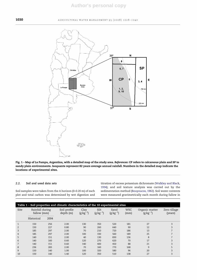
The present study was carried during 2004 on soils of the

calcareous (CP) and sandy plains (SP) of La Pampa, West of

Buenos Aires and South of Cordoba provinces (Fig. 1). These

two regions differ mainly due to their rainfall regime (ranging

from 600 to 700 mm per year), soil texture and soil profile

depth. The soils were entic and typic Haplustolls with

carbonate free A horizons.

Ten representative fields were selected that had been

cultivated with corn (Zeamays) under zero tillage in the previous

season, and showed contrasting soil texture and profile depth

(Table 1). The fallow period started in July with application of

herbicide (glyphosate) and finished in October or beginning of

November with seeding of a sunflower (Helianthus annuus) crop.

All sites had approximately three months of fallow. At the

beginning of the fallow period, three levels of crop residue cover

were established that represented the amount of remaining

stubble in different managements of corn crops in the typical

mixed production systems of the region. The exact dates of corn

harvest, glyphosate applications, establishment of residue

cover treatments and fallow period are shown in Table 2.

Treatment L (low) with less than 2000 kg DM ha�1 repre-

sented corn crops that were harvested and subsequent

intensive grazing of the stubble during winter; or silage corn

completely removed; or corn as green forage crop grazed

during summer. Treatment M (medium) had between 4000

and 6000 kg DM ha�1 and corresponded to grain crops whose

stubble is very lightly grazed. Treatment H (high) represented

corn grain crops with remaining stubble in the order of

10,000 kg DM ha�1. Treatment L was established by removing

excess residues, treatment M corresponded to the actual level

of stubble in these fields, and treatment H was achieved by

transporting the excess stubble from L to H. This meant that

while in treatment L and M the residue cover was actually

standing stubble, in treatment H some of the residue was flat

lying and therefore could be considered a mulch cover.

The treatments consisted of 10 m � 20 m plots in a

completely randomized block design with four repetitions;

plots were split in sub-treatments that consisted in (a) weed

control with 2.5 l glyphosate ha�1 and (b) no weed control at all

during fallow (see Table 2 for details).

a g r i c u l t u r a l w a t e r m a n a g e m e n t 9 5 ( 2 0 0 8 ) 1 0 2 8 – 1 0 4 0 1029


2.2. Soil and weed data sets

Soil samples were taken from the A horizon (0–0.20 m) of each

plot and total carbon was determined by wet digestion and

titration of excess potassium dichromate (Walkley and Black,

1934); and soil texture analysis was carried out by the

sedimentation method (Bouyoucos, 1962). Soil water contents

were measured gravimetrically each month during fallow in

Fig. 1 – Map of La Pampa, Argentina, with a detailed map of the study area. References: CP refers to calcareous plain and SP to

sandy plain environments. Isoquants represent 82 years average annual rainfall. Numbers in the detailed map indicate the

locations of experimental sites.

Table 1 – Soil properties and climatic characteristics of the 10 experimental sites

Site Rainfall duringfallow (mm)

Soil profiledepth (m)

Clay(g kg�1)

Silt(g kg�1)

Sand(g kg�1)

WSC(mm)

Organic matter(g kg�1)

Zero tillage(years)

Historical 2004

1 150 256 2.00 130 350 520 181 27 3

2 150 227 0.80 90 260 640 90 12 3

3 185 297 2.00 70 210 720 186 13 7

4 185 297 2.00 100 330 560 189 25 7

5 140 151 2.00 40 130 830 136 8 7

6 140 160 0.60 120 270 620 70 17 3

7 140 151 0.60 140 400 450 88 21 3

8 236 283 2.00 70 160 770 168 9 5

9 150 140 1.00 100 320 580 96 20 3

10 150 140 1.40 120 350 510 138 27 3



samples taken at 0.20 m depth intervals to 2.00 m depth or

to the depth of the calcite layer. Bulk density (BD) was

determined for each depth interval using soil samples taken in

steel cylinders of known volume. On these soil samples

permanent wilting point (PWP) and field capacity (FC) were

determined using the Richards pressure device.

Water storage capacity was calculated using the following

equation:

WSC ¼ profile depth� ðwater content at FC

�water content at PWPÞ � BD

Available water contents (AW) were calculated according to

the following equation:

AW ¼ profile depth� ðwater content�water content at PWPÞ

� BD

Fallow efficiency was calculated by the equation of

Mathews and Army (1960):

FE ¼ AW at the end of fallow�AW at the beginning of fallowrainfall during fallow

� 100

Soil temperature was taken each month at sites 1–8, while

at sites 9 and 10 weekly measurements at 0.05 m depth were

carried at 15:00 h out with digital thermometers. Air tem-

perature was taken at 15:00 h of the same day soil temperature

was measured. Details of the sampling scheme for soil

moisture and temperature at each site are given in Table 3.

The meteorological statistics of EEA INTA Anguil were

consulted in order to obtain data for historical average rainfall

(1921–2003) during fallow at the experimental sites. Rainfall

during the fallow period 2004 was recorded using officially

approved rain gauges at 1.5 m height at each site.

The amount of weed plants, separated by species, was

counted in 4 repetitions of 0.25 m2 in each treatment at the end

of the fallow period. For each residue level species richness

was calculated where this was simply the number of species

present in a sample, community, or taxonomic group

(McNaughton and Wolf, 1984).

Statistical analysis included ANOVA employing Tukey’s

test to determine differences between means, and regression

analysis, both using SAS software (SAS Institute, 1999). In

order to carry out an exploratory analysis of the relation

between residue levels and weed species a contingency table

was applied where the nil hypotheses was that weed species

have no homogeneous distribution among residue levels.

Since this hypothesis was accepted, a correspondence

analysis between weed species and residue level was carried

out. Comparison of regression lines was carried out according

to the method proposed by Sokal and Rohlf (1968).

3. Results

3.1. Site-specific conditions

The soils at the 10 sites differed considerably in profile depth

ranging from 0.60 to 2.00 m and also had very different

textures with sand contents between 450 and 830 g kg�1

(Table 1). These differences also were reflected in organic

matter contents that ranged from 8 to 28 g kg�1, with the

lowest values found in either very shallow or extremely sandy

soils. The soil’s WSC showed similar variability according to

texture and soil depth, ranging from a minimum of 70 mm to a

maximum of 189 mm. However, in contrast to what might

have been expected, sandy soils had higher WSC than loamy

soils, due to their deeper profiles. The sandy soils are mostly

found in the SP region where rainfall is higher and soil depth is

not limited by a calcite layer. Sites 3, 4, 5 and 8 belong to the SP

environment, whereas sites 1, 2, 6, 7, 9 and 10 are found in the

CP (Fig. 1), where soils have finer loamy textures but are

shallow due to the presence of calcite. The calcite layer at

0.60 m depth at site 6 (S6) limited the WSC of the soil to 70 mm,

whereas S4 due to its profile depth of 2.00 m had a WSC of

189 mm. Nevertheless S6 soil stores more water per volume

unit than S4.

Rainfall during the fallow period varied among sites

between 140 and 297 mm, following the climatic gradient

with higher values in the East of the region (SP) and lower

values in the West (CP), but in most cases there was more rain

during fallow than the historical average for this period.

Rainfall during fallow in sites 1, 3, and 4 was 100 mm higher

than this average; at sites 2, 5, 6, 7, and 8 this difference was

between 11 and 77 mm more rain, whereas at sites 9 and 10

rainfall was slightly lower than the historical average.

Table 2 – Time schedule of fallow, residue level (main plot) and weed control (subplot) establishment at each site (all datesare during 2004)

Site Corn harvest Establishmentof residue levels

Herbicide applications Total days Fallow period

First Second From To

1 March 24th July 14th July 14th September 9th 113 July 14th November 3rd

2 March 20th August 5th August 5th October 5th 107 August 5th November 19th

3 April 2nd July 6th July 6th September 5th 126 July 6th November 8th

4 April 6th July 6th July 6th September 5th 126 July 6th November 8th

5 April 10th August 5th August 5th October 10th 93 August 5th November 5th

6 March 28th August 10th August 10th October 15th 94 August 10th November 12th

7 March 26th August 11th August 11th October 15th 79 August 11th October 28th

8 April 5th July 16th July 16th October 12th 133 July 16th November 25th

9 March 21st July 8th July 8th October 5th 120 July 8th November 1st

10 March 23rd July 8th July 8th October 5th 120 July 8th November 1st



3.2. Management factors

The evolution of soil water contents during fallow, averaged

across all sites except S4 and 5 (Fig. 2) showed that weed

control (C) plots H residue treatments began to separate from

the second sampling period, while the difference between M

and L became evident in the third sampling period. Overall, a

tendency to store more water in H treatments could be

observed. In the subplots with no weed control (W) water

contents were only taken in the first and last sampling period

and a clear trend for water loss was observed in M and L

treatments, while H maintained initial water contents.

Table 4 shows the initial and final AW contents in the three

residue levels (H, M, L) separated according to weed control (C)

and weed (W) subplots. AW contents were calculated to a

uniform profile depth of 1.00 m, except for sites 2, 6 and 7 where

the effective depths were 0.80, 0.60 and 0.60 m respectively. At

the onset of the fallow period AW contents differed widely

among sites (Table 4). Site 5 had the highest value of 531 mm,

which was related to the presence of a water table at 2 m depth.

In general terms, initial AW was mostly determined by texture

and profile depth as well as by previous rainfall. The highest

differences between initial and final AW (Table 4) were found in

C H treatments at sites 1, 8 and 9 with values of 52, 71 and 58 mm

respectively. At sites 5 and 6 final AW was lower than initial AW.

In the W subplots final AW was below initial AW at most sites

even in the H treatments, and only at S1, S3, S8 and S9 there was

more AW at the end of fallow. On average, C H treatments had

16.4 mm more, and W H had 12.6 mm less AW at the end of

fallow than at the beginning.

In the weed control (C) subplots H had significantly higher

final AW contents than M and L at most sites, the exceptions

were S4, S5 and S6. The average AW content in the C plots

showed significant differences between all three levels, with

values of 90, 96 and 105 mm for L, M and H respectively. The

presence of weeds caused that no effect of residue levels was

noticeable at most sites, except at S1, S9 and S10. However, the

average AW contents showed a significant difference between

H and both other residue levels in W plots. In all cases except

S9 L treatment, AW contents of W subplots were significantly

lower than in C plots. The average difference between C and W

treatments was 29 mm AW.

At site 4 the farmer applied glyphosate to all plots;

therefore no W treatment could be analyzed. This site and

S5, due to the effect of a water table near the surface were

omitted from further analysis.

The data presented in Table 4 suggested that there might be

an interaction between residue and weed treatments; there-

fore we carried out an analysis of the effect of both factors on

final AW. Table 5 shows the final AW contents for the different

residue levels averaged across weed treatments and for weed

treatments averaged across residue levels. A significant effect

of weed control was found in all sites with an average

difference of 35 mm AW between control and weed plots.

Residue level also had a significant effect on AW in most sites

except sites 2, 3 and 8. The difference of AW between H and L

was 18.5 mm. When the interaction between weed control and

residue cover was analyzed for each residue level (Table 7), a

strong effect of weeds on AW could be found in most sites and

especially in M and L treatments.

Ta

ble

3–

Tim

esc

hed

ule

of

soil

mo

istu

rea

nd

soil

tem

pera

ture

mea

sure

men

tsa

tea

chsi

te

Sit

eS

oil

mo

istu

reS

oil

tem

pera

ture

114th

July

19th

Au

gu

st22n

dS

ep

tem

ber

3rd

No

vem

ber

19th

Au

gu

st22n

dS

ep

tem

ber

3rd

No

vem

ber

25th

Au

gu

st25th

Au

gu

st23rd

Sep

tem

ber

19th

No

vem

ber

25th

Au

gu

st23rd

Sep

tem

ber

19th

No

vem

ber

36th

July

3rd

Au

gu

st29th

Oct

ob

er

8th

No

vem

ber

3rd

Au

gu

st29th

Oct

ob

er

8th

No

vem

ber

46th

July

3rd

Au

gu

st29th

Oct

ob

er

8th

No

vem

ber

3rd

Au

gu

st29th

Oct

ob

er

8th

No

vem

ber

55th

Au

gu

st31st

Au

gu

st1st

Oct

ob

er

5th

No

vem

ber

31st

Au

gu

st1st

Oct

ob

er

5th

No

vem

ber

610th

Au

gu

st2n

dS

ep

tem

ber

4th

Oct

ob

er

12th

No

vem

ber

2n

dS

ep

tem

ber

4th

Oct

ob

er

12th

No

vem

ber

711th

Au

gu

st2n

dS

ep

tem

ber

4th

Oct

ob

er

12th

No

vem

ber

2n

dS

ep

tem

ber

4th

Oct

ob

er

12th

No

vem

ber

816th

July

27th

Au

gu

st21st

Sep

tem

ber

25th

No

vem

ber

27th

Au

gu

st21st

Sep

tem

ber

25th

No

vem

ber

98th

July

9th

,17th

,24th

Au

gu

st

2n

d,

6th

,14th

,

20th

,27th

Sep

tem

ber

5th

,12th

,18th

,

26th

Oct

ob

er

1st

No

vem

ber

9th

,17th

,24th

Au

gu

st

2n

d,

6th

,14th

,20th

,

27th

Sep

tem

ber

5th

,12th

,18th

,

26th

Oct

ob

er

1st

No

vem

ber

10

8th

July

10th

,19th

,

24th

Au

gu

st

1st

,6th

,15th

,

21st

,28th

Sep

tem

ber

7th

,14th

,19th

,

27th

Oct

ob

er

4th

No

vem

ber

10th

,19th

,

24th

Au

gu

st

1st

,6th

,15th

,21st

,

28th

Sep

tem

ber

7th

,14th

,19th

,

27th

Oct

ob

er

4th

No

vem

ber



Fallow efficiency among sites and between treatments

(Table 6) was extremely variable. Many sites even showed

negative FE (S 2, 6, 7 and 10), which was due to high initial AW,

near or above 100% of WSC, due to their shallow soil profile.

The highest FE was found in sites 9 and 10 (41 and 32.3%

respectively) followed by S1 and S8 (24.9 and 20.1% respec-

tively). All these sites had relative low initial AW compared

with their total WSC.

Table 4 – Initial and final available water contents (AW) in residue cover treatments with and without weed control

Site Initial AW (mm) Final AW Final AW

C (mm) W (mm)

L M H L M H

1 41 75 bA 76 bA 93 aA 61 bA 54.5 bB 85 aB

2 115 104 bA 106 bA 124 aA 42 aB 53 aB 55 aB

3 74 91 bA 102 aA 100 abA 74 aB 76 aA 84 aA

4 90 75 a 75 a 93 a – – –

5 209 137 aA 138 aA 132 aA 124 aA 127 aA 121 aA

6 89 61 aA 62 aA 66 aA 28 aB 35 aB 46 aB

7 82 77 bA 81 bA 89 aA 54 aB 57 aB 64 aB

8 70 124 bA 139 abA 141 aA 92 aB 89 aB 91 aB

9 47 79 bA 88 bA 105 aA 60 bA 52 bB 91 aB

10 79 76 bA 90 bA 107 aA 16 bB 39 abB 58 aB

Average 89.6 90 cA 96 bA 105 aA 62 bB 65 bB 77 aB

References: Available water contents measured in 1.00 m soil profile at the beginning (initial) and end (final) of fallow. Lower case letters indicate

significant differences between residue levels at each site within residue and weed treatments respectively. Uppercase letters refer to

significant differences between weed control (C) and weed (W) treatments at different levels of residue cover: high (H), medium (M) and low (L).

ANOVA at 90% confidence level.

Table 5 – Final available water contents in the experimental sites in different residue levels and with or without weedcontrol

Site Residue treatment Weed treatment

L M H C W

1 70.0 b 70.4 b 97.9 a 91.0 a 67.8 b

2 73.9 a 79.0 a 89.5 a 111.5 a 50.0 b

3 82.3 a 89.1 a 92.1 a 97.5 a 78.2 b

6 44.1 b 48.8 ab 55.9 a 63.0 a 31.2 b

7 65.7 b 69.3 ab 76.5 a 82.6 a 58.3 b

8 108.0 a 114.1 a 115.9 a 134.6 a 90.7 b

9 70.0 b 70.4 b 97.9 a 91.0 a 67.8 b

10 46.6 c 64.6 b 82.7 a 91.0 a 38.2 b

References: ANOVA at 90% confidence level. Residue treatment (R): H, high; M, medium; L, low; values are average of residue treatment with and

without weed control. Weed treatments (W): C, control; W, weeds; values represent the average of weed treatment through different residue

levels. Water contents expressed as mm of water in 1.00 m soil profile depth.

Fig. 2 – Evolution of available water contents during fallow in control (C) and weed (W) treatments. References: Represented

values are averages of all sites to a depth of 1.00 m. Sampling periods correspond to those detailed in Table 3. In W only

initial and final water contents were measured.



The effect of initial AW on FE was analyzed through

regression analysis separating C and W data (Fig. 3). In order to

represent soils with different WSC, AW data were transformed

to percentage of WSC (relative initial AW). A strong negative

relationship (R2 = 0.72) was observed for the C dataset, while

for W no such clear effect could be found (R2 = 0.23). While in

soils with complete weed control (C), the probability of

negative FE appeared at very high relative initial AW, in W

plots negative FE were to be expected at very low values (above

40% relative initial AW).

Residue level had a significant effect on FE in the same way

as on AW contents. Control H residue treatment had the

highest FE values in all sites. The average values for FE in C

plots were significantly different among the three residue

Table 6 – Fallow efficiency (FE) in residue cover treatments with and without weed control

Site FE (%) FE (%)

C W

L M H L M H

1 13.5 aA 13.5 bA 20.1 bA 7.7 aA 5.3 bB 17 bB

2 �4 aA �4.5 aA 3.5 aA �37.9 aB �30.2 aB �28.4 aB

3 5.7 bA 9.4 aA 8.7 abA �0.4 aB 0.6 aA 3.3 aA

6 �17.5 aA �16.9 aA �14.4 aA �31.8 aB �32.4 aB �27.3 aB

7 �3.2 bA �0.7 bA 4.2 aA �18.8 aB �16.6 aB �12.1 aB

8 19.2 bA 24.5 aA 24.9 aA 7.9 aB 7.2 aB 7.6 aB

9 23.5 aA 29.5 aA 41 aA 9.6 bA 3.8 bB 31.6 aB

10 10.3 bA 19.8 bA 32.2 aA �31.5 aB �15 aB �1.4 aB

Average 5.9 cA 9.3 bA 15 aA �11.9 bB �9.7 bB �1.2 aB

References: Fallow efficiency (FE) measured in 1.00 m soil profile. Lower case letters (a and b) indicate significant differences between residue

levels at each site within residue and weed treatments respectively. Uppercase letters (A and B) refer to significant differences between weed

control (C) and weed (W) treatments at different levels of residue cover: high (H), medium (M) and low (L). ANOVA at 90% confidence level.

Fig. 3 – Relation between initial available water contents and fallow efficiency in control (C) and weed (W) treatments.

References: Available water is expressed as percentage of WSC. Data represent average values of sites 1, 3, 7, 8, 9, and 10 to a

depth of 1.00 m. Sites where initial available water was above 100% WSC (S6 and S2) were excluded.

Table 7 – Statistical significance (p values) of the interaction between residue and weed treatments in different levels ofresidue

Site AW FE

L M H L M H

1 0.0770 0.0017 0.3000 0.0798 0.0017 0.3000

2 0.0030 0.0133 0.0019 0.0034 0.0176 0.0146

3 0.0639 0.0085 0.0877 0.0640 0.0086 0.0867

6 0.0010 0.0480 0.0200 0.0011 0.0048 0.0200

7 0.0066 0.0051 0.0038 0.0064 0.0054 0.0041

8 0.0002 <0.0001 <0.0001 0.0001 <0.0001 <0.0001

9 0.0800 0.0033 0.1900 0.079 0.0030 0.1900

10 0.0003 0.0012 0.0016 0.0003 0.0012 0.0015

References: ANOVA at 90% confidence level. Residue treatment: H, high; M, medium; L, low. AW: Available water; FE: fallow efficiency.



levels (5.9, 9.3 and 15% for L, M and H respectively). Weed

treatments showed significantly lower FE values at all sites,

and at half of these FE values were negative in W treatments

(Table 6). The effect of residue in W treatments was also less

important than in C plots; average values were�11.9,�9.7 and

�1.2% for L, M and H respectively and only H was significantly

different from both other residue levels. Nevertheless, in both

C and W, the difference in FE between L and H was around 10%.

The interaction between residue and weed treatments

(Table 7) was strongest in M and L, but at sites 7, 8 and 10

an important interaction was also observed in H treatments.

Weed density (Table 8) was significantly different between

residue levels at all sites. The highest differences between L

and H were observed at sites 1, 7, 9 and 10, with 65, 86, 43 and

50% fewer plants in H compared to L residue level. The average

values for L, M and H were 99, 71 and 54 plants m2 respectively,

which represented a 45% difference between H and L. Species

richness also decreased with the level of residue cover with

significant differences between L and H ( p < 0.05) (Table 8).

Forty eight species of weeds were found (Table 9); the most

abundant family was Compositae, followed by Umbiliferae and

Gramineae which represented 35, 15 and 13% of total

abundance respectively. The correspondence analysis

(Fig. 4) showed that H residue was defined by a reduced

number of species which were: Ammi majus, Onopordium

acanthium, Stellaria media, Chenopodium album and volunteer Z.

mays. For the case of M treatments weed composition

corresponded to: Salsola kali, Gnaphalium spicatum, Oenothera

mendocinesis, Trifolium repens, Cenchrus incertus and Hordeum

stenostachys. The higher correspondence with L residue level

was found with Sorghum halepense, Veronica peregrina var.

Xalepensis, Avena fatua, Polygonum aviculare, Specularia biflora,

Capsella bursapatoris, Bidens pilosa, Bowlesia incana, Lepidium

bonariensis, Aphanes parodii and Conyza bonariensis.

The effect of residue cover on soil temperature during one

day was analyzed at S1 on 3rd of November (Fig. 5).

Temperature was considerably lower in H than in L, this

difference was highest in the morning (almost 10 8C), then H

soil warmed to a difference of only 5 8C and maintained this

temperature during the early afternoon, whereas L warmed up

Table 8 – Density and species richness of weeds in the treatment without weed control for three levels of residues (L, M, H)

Site Density (plants m�2) Species richness (no.)

L M H L M H

1 75 a 56 a 26 b 8 16 12

2 72 a 59 a 44 a 12 12 15

3 80 a 57 a 55 a 7 8 7

6 122 a 100 a 89 a 12 15 18

7 85 a 36 ab 12 b 4 12 9

8 89 a 79 a 60 a 6 12 8

9 147 a 92 b 84b 4 11 11

10 119 a 71 ab 59 b 9 11 10

Average 99 a 71 ab 54 b 12 a 10 ab 8 b

Table 9 – List of weed species and their abbreviations

Species Abbreviation Species Abbreviation

Ammi majus AMIMA Lepidium bonariensis LEBPO

Aphanes parodii APHPA Licopsis arvensis LICAR

Avena fatua AVEFA Linaria texana LINTX

Bidens pilosa BIDPI Matricaria recutita MATCH

Bowlesia incana BOWIN Medicago mınima MEDMI

Bromus brevis BROBR Oenothera mendocinesis OEOME

Capsella bursa-pastoris CAPBP Onopordum acanthium ONRAC

Carduus acanthoides CRUAC Polygonum aviculare POLAV

Cenchrus incertus CCHIN Polygonum convolvulus POLCO

Centaurea solstitialis CENSO Portulaca oleracea POROL

Hordeum stenostachys HORST Rapistrum rugosum RASRU

Chenopodium album CHEAL Lolium multiflorum LOLMU

Cirsium vulgare CIRAR Rumex crispus RUMCR

Conyza bonariensis ERIBO Salsola kali SASKA

Cynodon dactylon CYNDA Sonchus oleracea SONOL

Cyperus rotundus CYPES Sorghum halepense SORHA

Descurainia argentina DESAR Specularia biflora TJDBI

Erodium cicutarium EROSCI Stellaria media STEPB

Euphorbia dentata EPHDE Taraxacum officinale TAROF

Gamochaeta calviceps GNACA Trifolium repens TRFRE

Gnaphalium gaudichaudianum GNAPE Veronica arvensis VERAR

Hypochoeris chillensis HRYCH Veronica peregrina var. Xalepensis VERPX

Lactuca serriola LACSE Vicia sativa VICSA

Lamiun amplexicaule LAMAM Zea mays ZEAMX



more from 12:00 h to the last measurement at 14:30, when the

difference between both treatments was again about 10 8C.

At sites 9 and 10, where a complete set of soil temperature

data was taken, we analyzed the relation between soil and air

temperature for L, M and H residue levels (Fig. 6). As expected,

all treatments, averaged across both sites, showed strong

relationships with R2 of 0.76, 0.75 and 0.81 for L, M and H

respectively.

3.3. Empirical model

In order to evaluate the effect of the site-specific and

management factors on water storage during fallow we

developed a simple empirical model. As independent variables

water storage capacity, rainfall, soil profile depth, weed

control, and residue level, were used to predict final AW

contents. Different functional dependencies were tested

applying the parsimony principal. The best result was

obtained with the following equation:

W ¼ p0 þ p1WCþ p2RL2 þ p3WSC2 þ p4Rþ p5R2 þ p6eD

W is final AW content, and pi are the corresponding model

parameters. WC is the weed control; the data used were the

number of weed plants in W treatments and a 0 was assigned

as value for C treatments. RL is the residue level; values of 2, 5

and 10 Mg ha�1 were used for L, M and H respectively. WSC is

the water storage capacity of each site in mm. R is the rainfall

during fallow 2004 in mm at each site.D is the soil profile depth

in m at each site.

The model parameters were calculated using the least

square method. Due to the fact, that the number of samples

was small, the prediction quality of the empirical model was

analyzed by using the cross-validation method. Here one data

set is left out for the model parameter calculation. Using these

model parameters, the left out data set is used to predict the

water content as well as to calculate the error with respect to

the corresponding water content measurement. This is

performed with all data sets successively. The data from

one experimental site with the three levels of residue were

used as one data set. Therefore, 16 different data sets were

Fig. 4 – Biplot based on correspondence analysis with residue cover as (+) and species as (&). See Table 9 for abbreviations.

Fig. 5 – Evolution of soil temperature during the day under L

and H residue levels. References: Data represent values

from site 1 on November 3rd. Soil temperature was

measured at 0.05 m depth.



obtained, each with 3 different levels of residue, which gives a

total of 48 individual predicted values of the water content. For

the calculation of the average error of the cross-validation

method the following equation was used:

E ¼P48

i¼1 jWi �Wij=Wi

48� 100

E is the average percentage error of prediction of the water

content; Wi and Wi are the ith predicted and measured water

content values respectively. An average percentage prediction

error of 19.7% was obtained; this was considered an acceptable

error.

The average model parameter values as well as their

percentage error obtained from the 16 data sets of the cross-

validation are presented in Table 10. The two highest errors of

the parameters corresponded to rainfall with its linear and

quadratic term respectively. The smallest error corresponded

to weed control, which indicated a stable influence of this

variable for the empirical model. Another very significant

parameter was WSC with the second lowest error. The factor

with the highest parameter value was rainfall, although its

error was very high, indicating an erratic but strong effect on

water storage. When the average model parameter values

were used, an overall average percentage error of prediction

13.7% was obtained. In this calculation the values of site 6 for

no weed control had individual errors of above 40%. If they are

not considered in the average percentage error of prediction,

an error of only 12% was obtained. A scatter plot of all

predicted values by the empirical model and the measured

values is shown in Fig. 7. The values distributed quite well

around the optimal graph, and the determination coefficient

of the data (R2 = 0.77) indicated an acceptable correspondence.

However, one has to keep in mind, that it is an empirical data

driven model, where no functional aspects are considered.

Therefore, the interpretation of the model is restricted; and

although an interpolation can be carried out, an extrapolation

is not suggested.

Fig. 6 – Relation between soil and air temperature in three residue cover treatments. References: Data are averaged across

values of sites 9 and 10.

Fig. 7 – Regression plot of measured and predicted values of

the empirical model.

Table 10 – Parameter values of the empirical model obtained as average values from the 8 experimental sites for C and Wplots (total n = 16) during the cross-validation method as well as their corresponding percentage errors

Modelparameter

p0

(mm)p1

(mm/plants m�2)p2

(mm/Mg2)p3

(mm/mm2)p4

(mm/mm)p5

(mm/mm2)p6

(mm)

Average 172 �0.460 0.0702 �0.0044 �1.12 0.0030 20.

Percentage error 13.5 5.7 14 10.6 22.2 18.6 12.6

References: p0, general model parameter; p1, weed control; p2, residue level; p3, water storage capacity; p4, rainfall; p5, (rainfall)2; p6, profile depth.



4. Discussion

Site-specific soil conditions such as WSC and profile depth

affected water storage during fallow, as was shown by the

empirical model (WSC had the second lowest error) and also by

final AW data; the highest values corresponded to sites 1, 3, and

8, which had the deepest profiles and highest WSC. Various

previous studies already mentioned this positive effect of soil

depth and WSC on water storage during fallow (Moret et al.,

2005; Lampurlanes et al., 2002; Tanaka and Aase, 1987).

However, FE data did not reflect this trend; for this variable,

initial AW contents apparently had a stronger effect, since the

highest FE values were found at sites with lowest initial AW

(sites 1, 9, 10). In spite of this interaction, initial AW was not a

useful model parameter, and did not improve the prediction

error of the model. Another site-specific factor that showed a

strong effect was the amount of rainfall during fallow. Sites 1, 3

and 8 had highestamounts of rainand alsohighestfinalAW. For

FE, an interaction between initial AW and amount of rain during

fallow could exist, which might explain that sites with lowest

values for both factors had the highest FE.

Residue level had a positive effect on water storage in both

control and weed treatments. In weed control plots a stronger

effect of residue level was found, while with no weed control

only at the highest residue level a difference was observed.

The same trend was also found for FE values. The model takes

into account a quadratic factor for residue level. This was

necessary since residue cover was expressed as the average

dead biomass on the plots in units of Mg ha�1, which are

relatively small values compared to other model parameters.

However, the relatively high error of this parameter would

indicate that the effect of residue level was not as strong as

other parameters.

The model parameter with the lowest error was weed

control, which indicated that the amount of weeds had a very

strong and uniform effect on water storage. The ANOVA also

showed that the effect of weed was more significant than that

of residue level. The strong interaction between weed and

residue treatments for both final AW and FE indicated that

there might have occurred weed suppression due to high

residue cover. In each treatment the sub-treatment without

weed control had lower water contents than C plots. This

could be explained by an interaction between water use by

weeds and higher evaporation rates due to higher soil

temperatures. High weed populations in L residue treatments

could be related to the fact that higher temperatures might

have favored germination of weeds (Shafii and Price, 2001;

Garcıa Huidobro et al., 1982), and low soil temperatures caused

by high residue cover could affect germination and emergence

of plants (Munawar et al., 1990; Al-Darby and Lowery, 1987;

Griffith et al., 1973). Therefore high residue treatments also

would conserve more water during fallow due to the

suppression of weeds, resulting in higher FE. Weed species

composition among residue levels was different as shown by

the correspondence analysis. These results indicated that

weed species apparently have different requirements for

germination and some are more efficiently suppressed by

residue cover than others. The case of C. album, which was

found to be associated with H residue level in our experi-

mental conditions showed the degree of uncertainty about the

factors that affect weed suppression. This species was

reported to be suppressed by cover crops (Teasdale et al.,

1991) while other studies found no effect of residue cover

(Moore et al., 1994) on its emergence. We expected Chenopo-

dium to be more frequent in L treatments due to its light

requirements for germination (Bouwmeester and Karssen,

1993; Gallagher and Cardina, 1998).

The interaction between WSC, rainfall during fallow,

residue level and weed control and their effect on FE was

most clearly observed in site 10: FE increased from 10% in L to

32% in treatment H. At this site, rainfall during fallow was less

than historical average, while at sites with higher than average

rainfall during fallow the effect of residue on FE was not as

strong. Power et al. (1986) already observed that the effect of

residue cover on water storage was most important in dry

years. At this site the effect of weed suppression by residue

cover on final AW was very important, resulting in almost

twice the amount of AW in weed control compared to weed

plots. Although all treatments at site 9 also had very high FE,

this site did not show the same response to residue level as

S10, although both received equal amounts of rainfall during

fallow. This might have been due to the considerably lower

WSC of S9 caused by the combination of lower profile depth

and a slightly more sandy texture.

The empirical model was useful to identify the factors that

had a strong effect on water storage during fallow. The most

determinant factor under our experimental conditions was

weed control, followed by rainfall during fallow, which despite

the high prediction error had high parameter values. We

attempted to use the model equation for predicting final AW,

substituting rainfall with the corresponding historical mean

values for each site. The resulting determination coefficient of

the regression between measured and predicted values

dropped to R2 = 0.50, which for practical purposes is not

useful. This certainly is due to the high variability of average

rainfall values. Nevertheless, more studies under different

climatic conditions are needed to further improve and validate

this model for prediction of water storage during fallow.

Our results showed that it is feasible to obtain higher than

30% FE in semiarid regions, especially in situations where little

rainfall occurs during fallow in soils with high WSC; weed

control and high residue cover enhance this effect. Thus in

sites 9 and 10 treatment H stored 55 and 44 mm respectively of

all rainfall occurred during fallow, which resulted in a

significant increase of crop available water.

The interaction between residue level and weed control

showed that the mean difference between final AW of residue

treatments was only 18.5 mm, whereas the mean difference

between W and C for all residue levels was 35 mm. For

practical purposes these results show that chemical weed

control is more effective for improving FE than residue cover.

High residue levels showed to suppress weed density, but the

effect on water storage was by far not as effective as a

complete weed control. Nevertheless, the use of high residue

covers for a certain degree of weed control and to improve

water availability could be considered in subsistence and low

input systems. This also holds true for sites with very shallow

soil profiles (S6 and 7), where FE were all negative even at H

residue, and crop productivity might be so low as not to

compensate for herbicide costs.



Residue and mulch covers decrease soil temperature (Creus

et al., 1998); our data confirmed this effect. Treatment L had

higher soil temperature than H during the course of the day,

which indicated that residue cover in H plots impeded further

warming of the soil by solar radiation, due to an insulation

effect and possibly also a higher albedo. Lower temperatures

under high residue treatments would have lower evaporation

rates, thus contributing to water conservation during fallow.

The relation between soil and air temperature in different

treatments also confirmed this trend, as shown by higher

slope in H, compared with L and M. Statistical comparison of

these regression lines showed that L was significantly

different from H with regards to their slope and origin.

Apparently high residue cover acted as an insulation or buffer

between air and soil temperature. This might have been

caused by the high solar reflectance and low thermal

conductivity of stubble (Al-Darby and Lowery, 1987). This

buffer effect, however, also implies a drawback for crop

management, since the soils under H treatments reached the

same temperature of L treatments about 10–15 days later.

Therefore it could be expected that germination of the

subsequent crop would be slower in H; this should be taken

into account by delaying seeding dates in soils with high

residue cover.

For all statistical analysis AW data were uniformed to a

depth a 1.00 m, although measurements were carried out to

real profile depth or to a depth of 2.00 m where profiles were

deeper. We therefore wondered whether in deep soils such as

those at sites 1, 3, and 8, final AW and FE measured to a depth

of 1.00 m reflected the effective water storage during fallow.

When these values were compared with the soil water content

to 2.00 m depth important increases of FE were found. Thus at

S1 FE increased from 20 to 53% in treatment H, and at S3 and S8

similar differences between both depths were found. In these

deep soils the mayor contribution to FE apparently was

through the water stored at greater depth. The practical

implication was that crops with deep root systems explore the

soil profile to a depth of 2 m and could utilize this water

reserve. This would be the case of sunflower, for instance,

which can reach rooting depth of more than 2 m, while

soybean generally does not root deeper than 1.30 m in the

semiarid central region of Argentina (Dardanelli et al., 1997).

There are also considerable differences in rooting depth

among cultivars of the same crop species, and generally those

with a short growing period tend to have shallower roots than

those with long period. Our results therefore indicated that in

soils with similar texture and profile depth as sites 1, 3 and 8

crop rooting depth should be taken into account in order to

increase water use efficiency in these environments.

5. Conclusions

The empirical model described the interaction between site-

specific and management dependent factors for water storage

during fallow and an acceptable degree of agreement between

measured and predicted values was achieved. The most

determinant factor was weed control, followed by water

storage capacity. A strong interaction between residue level

and weed control was observed at all sites, implying weed

suppression by residue cover. However, for practical purposes,

chemical weed control was more effective for water storage

than residue cover, and using high residue cover for improving

fallow efficiency could only be valid for low input systems or at

sites with very low water storage capacity, where crop

productivity would not compensate for herbicide costs. High

residue cover also caused lower soil temperatures, which

could be considered a drawback for crop management since

seedling emergence would be slower or seeding dates would

have to be delayed.

Weed density and floristic composition was affected by

residue cover, and an association between certain weed

species and residue level was found. However, no functional

explanation of suppression of different species could be

arrived at.

Further studies are needed to improve and validate the

empirical model, in order to better understand the complex

interactions between site-specific and management factors.

r e f e r e n c e s

Aase, J., Pikul Jr., J., 2000. Water use in a modified summer fallowsystem on semiarid northern Great Plains. Agric. WaterManage. 43, 345–357.

Al-Darby, A.M., Lowery, B., 1987. Seed zone soil temperatureand early corn growth with three conservation tillagesystems. Soil Sci. Soc. Am. J. 51, 768–774.

Ballare, C.L., Casal, J.J., 2000. Light signals perceived by cropsand weed plants. Field Crops Res. 67, 149–160.

Bennie, A., Hensley, M., 2000. Maximizing precipitationutilization in dryland agriculture in South Africa, a review. J.Hydrol. 241, 124–139.

Black, A., Bauer, A., 1988. Strategies for storing and conservingsoil water in the northern Great Plains. In: Unger, P.W.,Jordan, W., Sneed, T.V. (Eds.), Challenges in DrylandAgriculture: A Global Perspective. Proceedings of theInternational Conference on Dryland Agriculture, Amarillo,TX, August 1988, Texas Agricultural Experiment Station,College Station, TX, USA, pp. 137–139.

Bouwmeester, H.J., Karssen, C.M., 1993. Seasonal periodicity ingermination of seeds of Chenopodium album L. Ann. Appl.Bot. 72, 462–473.

Bouyoucos, G., 1962. Hydrometer method improved for makingparticle size analyses of soils. Agron. J. 54, 464–465.

Creus, C., Studdert, G., Echeverria, H., Sanchez, S., 1998.Descomposicion de residuos de cosecha de maız y dinamicadel nitrogeno en el suelo. Ciencia del Suelo (Argentina) 16,51–57.

Dardanelli, L., Bachmeier, O., Sereno, R., Gil, R., 1997. Rootingdepth and soil water extraction patterns of different cropsin a silty loam Haplustoll. Field Crops Res. 54, 29–38.

Gallagher, R.S., Cardina, J., 1998. Phytocrome-mediatedAmaranthus germination. l: Effect of seed burial andgermination temperature. Weed Sci. 46, 48–52.

Garcıa Huidobro, J., Monteith, J., Squire, G., 1982. Time,temperature, and germination of pearl millet (Pennisetumtyphoides S. & H.). J. Exp. Bot. 33, 288–296.

Griffith, D., Mannering, J., Galloway, H., Parsons, S., Richey, C.,1973. Effect of eight tillage-planting systems on soiltemperature, percent stand, plant growth, and yield of cornon five Indiana soils. Agron. J. 65, 321–326.

Huang, M., Shao, M., Zhang, L., Li, Y., 2003. Water efficiency andsustainability of different long-term crop rotation system inthe Loess Plateau of China. Soil Till. Res. 72, 95–104.



Kohli, R.K., Batish, D., Singh, H.P., 1998. Allelopathy implicationsin agroecosystems. J. Crop Prod. 1, 169–202.

Lampurlanes, J., Angas, P., Cantero-Martınez, C., 2002. Tillageeffects on water storage during fallow, and on barley rootgrowth and yield in two contrasting soils of the semi-aridSegarra region Spain. Soil Till. Res. 65, 207–220.

Mathews, O., Army, T., 1960. Moisture storage on fallowwheatland in the Great Plains. Soil Sci. Soc. Am. Proc. 24,414–418.

Mc Aneney, K., Arrue, J., 1993. A wheat-fallow rotation innortheastern Spain: water balance-yield considerations.Agronomie 13, 481–490.

McNaughton, S.J., Wolf, L.L., 1984. Ecologıa General. Universidadde Siracusa. Ediciones Omega, S.A. Platon 26, Barcelona,Espana, 713 pp.

Moore, M.J., Gillespie, T.J., Swanton, C.J., 1994. Effects of covercrop mulches on weed emergence, weed biomass, andsoybean (Glycine max) development. Weed Technol. 8, 512–518.

Moret, D., Arrue, L., Lopez, M., Garcia, R., 2005. Influence offallowing practices on soil water and precipitation storageefficiency in semiarid Aragon (NE Spain). Agric. WaterManage. 82, 161–176.

Munawar, A., Blevins, R.L., Frye, W.W., Saul, M.R., 1990. Tillageand cover crop management for soil water conservation.Agron. J. 82, 773–777.

Pearson, T.R.H., Burslem, D.F.R.P., Mullins, C.E., Dalling, J.W.,2003. Functional significance of photoblastic germination inneotropical pioneer trees: a seed’s eye view. Funct. Ecol. 17,394–402.

Power, J., Wilhelm, W., Doran, J., 1986. Crop residue effects onsoil environment and dryland maize and soya beanproduction. Soil Till. Res. 8, 101–111.

SAS Institute Inc., 1999. SAS online doc. Statistics. Version 8 (TSM0). SAS Institute Inc., Cary, NC, USA.

Shafii, B., Price, W., 2001. Estimation of cardinal temperatures ingermination data analysis. J. Agric. Biol. Environ. Stat. 6,356–366.

Sokal, R., Rohlf, F., 1968. Biometrıa. Principios y metodosestadısticos en la investigacion biologica. H. BlumeEdiciones, Madrid, Espana.

Steiner, J., 1988. Simulation of evaporation and water useefficiency of fallow-based cropping systems. In: Unger, P.,Jordan, W., Sneed, T.V. (Eds.), Challenges in DrylandAgriculture: A Global Perspective. Proceedings of theInternational Conference on Dryland Agriculture, Amarillo,TX, August 1988, Texas Agricultural Experiment Station,College Station, TX, USA, pp. 176–178.

Tanaka, D., Aase, J., 1987. Fallow method influences on soilwater and precipitation storage efficiency. Soil Till. Res. 9,307–316.

Teasdale, J.R., 1996. Contribution of cover crops to weedmanagement in sustainable agricultural systems. J. Prod.Agric. 9 (4), 475–479.

Teasdale, J.R., Beste, C.E., Potts, W.E., 1991. Response of weeds totillage and cover crops residue. Weed Sci. 39, 195–199.

Walkley, A., Black, A., 1934. An examination of the Degtjareffmethod for determining soil organic matter and a proposedmodification of the chromic acid titration method. Soil Sci.37, 29–37.


A study of the effect of the interaction between site-specific conditions, residue cover and weed...

Documents

Transcript of A study of the effect of the interaction between site-specific conditions, residue cover and weed...