a study of groundwater contamination and bioremediation ...

Glasgow Theses Service http://theses.gla.ac.uk/

[email protected]

Metwaly, Hassan Ali Hassan (1999) A study of groundwater contamination and bioremediation treatment using natural soil and vegetation. PhD thesis. http://theses.gla.ac.uk/2851/ Copyright and moral rights for this thesis are retained by the author A copy can be downloaded for personal non-commercial research or study, without prior permission or charge This thesis cannot be reproduced or quoted extensively from without first obtaining permission in writing from the Author The content must not be changed in any way or sold commercially in any format or medium without the formal permission of the Author When referring to this work, full bibliographic details including the author, title, awarding institution and date of the thesis must be given

A STUDY OF GROUNDWATER CONTAMINATION AND BIOREMEDIATION TREATMENT USING NATURAL

SOIL AND VEGETATION

By HASSAN ALI HASSAN METWALY

M. Sc. (Hons) IN SOIL SCIENCE MINIA UNIVERSITY, EGYPT

THESIS SUBMITTED FOR THE DEGREE OF DOCTOR OF PHILOSOPHY

SEPTEMBER, 1999.

AGRICULTURAL, FOOD, AND ENVIRONMENTAL CHEMISTRY DEPARTMENT

FACULTY O`. SCIENCE UNIVERSITY OFLASGOW

UNITED KINGDOM

- IN THE NAME OF ALLAH "THE MOST GRACIOUS, THE MOST MERCIFUL"

"He Who taught (the use of) the pen, " "Taught man that which he knew not. "

ACKNOWLEDGEMENTS

With sincere words of thanks to the Most Compassionate, the Most Gracious

and the Most Merciful, ALLAH Who blessed me, helped me and gave me a light in the

road of knowledge.

I wish to express the deepest appreciation and gratitude to my supervisor, Dr.

T. H. Flowers for his constant support, continual help and advice throughout the work

covered in this thesis. Without his careful attention and encouragement throughout my Ph. D. this thesis could never has been completed.

I am extremely grateful to Dr. H. J. Duncan, Dr. I. D. Pulford, and Dr. Jarvis for their sincere help and advice during the course of this work. Their encouragement

and support have been of great value to me and appreciated. I wish to thank all colleagues and friends both past and present who have been

of assistance in my ways. I am extremely grateful to the Ministry of Higher Education in Egypt and to

all the staff of the Egyptian Educational and Cultural Bureau, Embassy of Arab

Republic of Egypt, in London, especially Prof. Mohammed Abd El-Hamid El-Sharkawy

for their encouragement, sincere help and financial support of my study and living.

I am extremely grateful to all the staff members of the Soil Science Department, Faculty of Agriculture, Minia University, Egypt, for their sincere help and

advice. Their encouragement and support have been of great value to me and appreciated.

I wish to thank Mr. Robert Craig for his help in collecting my groundwater

and soil samples from the Ardeer site, Mr. Fulton Murdoch for his help with analysis by

Inductively Coupled Plasma (ICP) Spectroscopy, and Mrs. Janet Harris, Environmental

Scientific Officer, for the information relating to the Ardeer site she supplied. I am extremely grateful to my father and the soul of my mother for their

sincere help, support and encouragement throughout my life.

I am extremely grateful to my wife for her constant patience, support and

encouragement.

Finally, I wish to express my sincere thanks to my 8 months old daughter Omnia Hassan Ali Hassan for keeping quiet.

I

CONTENTS

SUBJECT PAGE No.

ACKNOWLEDGEMENTS I

CONTENTS II

SUMMARY X

CHAPTER 1: GENERAL INTRODUCTION 1

1.1. NITROGEN CYCLE I

1.1.1. PLANT UPTAKE 3

1.1.2. MINERALISATION / IMMOBILISATION 4

1.1.3. DENITRIFICATION 5

1.1.4. AMMONIA VOLATILISATION 6

1.1.5. NITROGEN FIXATION 6

1.1.6. NITRIFICATION 6

1.1.6.1. FACTORS AFFECTING NITRIFICATION AND MINERALISATION 7

1.1.6.2. INHIBITION OF NITRIFICATION 8

1.2. GROUNDWATER QUALITY 10

1.2.1. SOURCES OF GROUNDWATER CONTAMINATION 11

1.2.2. IRRIGATION WATER QUALITY PROBLEMS 15

1.2.3. WATER QUALITY PARAMETERS AND EVALUATION 22

1.3. BIOREMEDIATION TREATMENT OF AMMONIUM AND 27

NITRATE CONTAMINATED GROUNDWATER

1.3.1. BIOREMEDIATION TECHNOLOGIES 28

1.3.1.1. DENITRIFICATION 29

1.3.1.2. PHYTOREMEDIATION OF INORGANIC CONTAMINATION 30

1.3.1.2.1. PHYTOREMEDIATION OF NITROGEN CONTAMINATED 32

WATER USING GRASS.

1.4. OBJECTIVES OF THESIS 34

II

CHAPTER 2: MATERIALS AND METHODS 37

2.1. CLEANING OF GLASSWARE AND PLASTICWARE 37

2.2. PURIFICATION OF THE FILTER PAPER TO REMOVE NITROGEN 39

CONTAMINATION

2.3. MEASUREMENT OF SOIL pH 39

2.4. MEASUREMENT OF WATER pH 40

2.5. MEASUREMENT OF THE ELECTRICAL CONDUCTIVITY (EC) 40

OF SOIL

2.6. MEASUREMENT OF THE ELECTRICAL CONDUCTIVITY (EC) 40

OF WATER

2.7. DETERMINATION OF MOISTURE CONTENT OF SOIL 41

2.8. DETERMINATION OF SOIL ORGANIC MATTER BY LOSS ON 41

IGNITION

2.9. DETERMINATION OF THE SOIL MOISTURE CONTENT AT -0.5 42

BAR SOIL MOISTURE POTENTIAL

2.10. SOIL MECHANICAL ANALYSIS 42

2.11. DETERMINATION OF MACRONUTRIENTS IONS 46

2.11.1. AUTOMATED DETERMINATION OF SOIL INORGANIC 46

NITROGEN

2.11.1.1. STANDARD METHOD FOR AMMONIUM NITROGEN 46

DETERMINATION (BERTHELOT METHOD)

2.11.1.2. DETERMINATION OF AMMONIUM-N (TOTAL NITROGEN) 49

IN KJELDAHL DIGESTS

2.11.1.3. AUTOMATED DETERMINATION OF NITRATE AND NITRITE 51

NITROGEN

2.11.2. AUTOMATED DETERMINATION OF SOIL INORGANIC 55

PHOSPHORUS

2.11.3. DETERMINATION OF POTASSIUM IN SOIL AND WATER 59

2.11.4. DETERMINATION OF SODIUM IN WATER 60

2.11.5. DETERMINATION OF CALCIUM IN SOIL AND WATER 60

2.11.6. DETERMINATION OF MAGNESIUM IN SOIL AND WATER 61

2.12. DETERMINATION OF TOTAL METALS BY THE ATOMIC 62

in

ABSORPTION SPECTROPHOTOMETER

2.13. FLAME CONDITIONS OF ANALYSIS BY THE ATOMIC 67


2.14. ANALYSIS OF METALS BY INDUCTIVELY COUPLED PLASMA 68

SPECTROSCOPY

2.15. DETERMINATION OF ANIONS BY ION CHROMATOGRAPHY 70

2.16. DETERMINATION OF CATION EXCHANGE CAPACITY IN SOIL 72

2.17. EXTRACTION OF INORGANIC NITROGEN FROM SOIL 74

2.18. EXTRACTION OF PHOSPHATE FROM SOIL 75

2.19. EXTRACTION OF POTASSIUM AND MAGNESIUM FROM SOIL 76

2.20. ACID DIGESTION OF SOIL 77

2.21. TOTAL NITROGEN IN PLANT MATERIAL 78

CHAPTER 3: METHODS DEVELOPMENT AND ASSESSMENT 82

3.1. AMMONIUM ANALYSIS IN SOIL AND WATER 82

3.1.1. INTRODUCTION 82

3.1.2. MATERIALS AND METHODS 92

3.1.2.1. METHOD DEVELOPMENT 92

3.1.2.1.1. SAMPLE FLOW RATE 92

3.1.2.1.2. OPTIMISATION OF THE REAGENTS, REACTION 92

CONDITIONS AND THE SELECTION OF THE SUITABLE

METHOD OF ANALYSIS

3.1.2.1.3. ASSESSMENT OF THE PRECISION OF THE OPTIMISED 99

METHOD FOR THE AMMONIUM DETERMINATION

3.1.3. RESULTS AND DISCUSSION 100

3.1.3.1. OPTIMISATION OF REAGENTS, REACTION CONDITIONS AND 100

THE SELECTION OF THE SUITABLE METHOD OF ANALYSIS

3.1.3.2. FINAL METHOD FOR THE DETERMINATION OF AMMONIUM 116

3.1.3.3. ASSESSMENT OF THE PRECISION OF THE OPTIMISED 120

METHOD FOR THE AMMONIUM DETERMINATION

N

3.2. DETERMINATION OF LOW LEVELS OF AMMONIUM 121

(< 0.1 mg N/ 1) IN GROUNDWATER



3.2.2.1. METHOD DEVELOPMENT 124

3.2.2.2. ASSESSMENT OF THE PRECISION OF THE FINAL METHOD 132


3.2.3.1. EFFECT OF THE POTASSIUM SODIUM TARTRATE AND 135

SODIUM CITRATE CONCENTRATIONS ON THE SOLUBILITY

OF THE HIGH CONCENTRATION COMPLEXING REAGENT

SOLUTION

3.2.3.2. ASSESSMENT OF THE PULSE SUPPRESSER TUBES 136

3.2.3.3. INFLUENCE OF THE SEQUENCE OF ADDING REAGENTS ON 136

THE PROPOSED METHOD

3.2.3.4. ASSESSMENT OF THE SAMPLE LINE DEBUBBLER 137

3.2.3.5. FINAL METHOD FOR THE DETERMINATION OF LOW 139

LEVELS OF AMMONIUM-N IN GROUNDWATER

3.2.3.6. ASSESSMENT OF THE PRECISION OF THE FINAL METHOD 142

3.3. ANALYSIS OF HIGHLY COLOURED GROUNDWATER SAMPLES 143



3.3.2.1. USING CHARCOAL G60 AND POLYCLAR SB 100 FOR THE 146

DECOLORISATION OF WATER SAMPLES

3.3.2.1.1. EFFICIENCY OF CHARCOAL G60 AND POLYCLAR SB 100 146

IN THE DECOLORISATION OF WATER SAMPLES

3.3.2.1.2. THE PRESENCE OF IMPURITIES IN CHARCOAL G60 AND 147

POLYCLAR SB 100

3.3.2.1.3. CLEANING CHARCOAL G60 AND POLYCLAR SB 100 FROM 149

IMPURITIES

3.3.2.1.4. ADSORPTION OF NH4-N AND N03-N FROM SOLUTION BY 152

THE CLEANED CHARCOAL G60 OR POLYCLAR SB 100

3.3.2.1.5. PREVENTION OF N03-N AND NH4-N ADSORPTION BY THE 153

V

CLEANED POLYCLAR SB 100 USING K2SO4 SOLUTION

3.3.2.2. INCLUSION OF A DIALYSIS SYSTEM WITH THE TECHNICON 155

AUTOANALYZER II FOR THE ANALYSIS OF GROUNDWATERS


3.3.3.1. USING CHARCOAL G60 AND POLYCLAR SB 100 FOR THE 164

DECOLORISATION OF THE WATER SAMPLES

3.3.3.2. INCLUSION OF A DIALYSIS SYSTEM WITH THE TECHNICON 175


3.3.3.2.1. INCLUSION OF THE LIQUID PHASE DIALYSIS FOR THE 175

DETERMINATION OF NITRATE AND NITRITE IN THE

GROUNDWATER SAMPLES

3.3.3.2.2. FINAL METHOD FOR THE DETERMINATION OF NITRATE 179

AND NITRITE IN THE GROUNDWATER SAMPLES

3.3.3.2.3. INCLUSION OF THE LIQUID PHASE DIALYSIS FOR THE 181

DETERMINATION OF CHLORIDE IN THE GROUNDWATER

SAMPLES

3.3.3.2.4. FINAL METHOD FOR THE DETERMINATION OF CHLORIDE 182

IN THE GROUNDWATER SAMPLES

CHAPTER 4: INVESTIGATION OF GROUNDWATER DUALITY AND 186

SOILS IN THE ARDEER SITE

4.1. INTRODUCTION 186

4.2. MATERIALS AND METHODS 199

4.2.1. WATER QUALITY PARAMETERS 199

4.2.1.1. WATER SAMPLING 199

4.2.1.2. GROUND WATER SURVEYS 203

4.2.2. CHARACTERISATION OF SOILS 211

4.2.2.1. SOIL SAMPLING 211

4.3. RESULTS AND DISCUSSION 224


4.3.1.1. pH 224

4.3.1.2. AMMONIUM-N 224

VI

4.3.1.3. NITRATE-N

4.3.1.4. NITRITE-N

4.3.1.5. CHLORIDE

4.3.1.6. SODIUM

4.3.1.7. POTASSIUM

4.3.1.8. CALCIUM

4.3.1.9. MAGNESIUM

4.3.1.10. IRON

4.3.1.11. ELECTRICAL CONDUCTIVITY

4.3.2. CHARACTERISATION OF THE SOIL

4.3.2.1. CHEMICAL AND PHYSICAL CHARACTERISTICS OF THE SOILS

4.3.2.1.1. INTERMEDIATE OXIDATION PLANT (IOP) AREA

4.3.2.1.2. H-ACID AREA

4.3.2.1.3. SAFETY FUSE AREA

4.3.2.1.4. NYLON AREA

4.3.2.2. ASSESSMENT OF THE TOXICITY AND THE HAZARDS OF THE

HEAVY METALS

4.3.2.3. OVERALL ASSESSMENT OF THE AREAS

CHAPTER 5-: NITRIFICATION IN SOIL TREATED WITH

CONTAMINATED GROUNDWATER

5.1. INTRODUCTION

5.2. MATERIALS AND METHODS

5.2.1. MATERIALS

5.2.1.1. SOIL SAMPLES

5.2.1.1.1. SOIL SAMPLING

5.2.1.2. GROUNDWATER WELLS

5.2.1.2.1. WATER SAMPLING

5.2.2. NITRIFICATION EXPERIMENTS

5.2.2.1. PRELIMINARY EXPERIMENT : NITRIFICATION RATE IN

SOILS TREATED WITH AMMONIUM SULPHATE AT

100 mg NH4-N /kg SOIL

225

226

233

233

234

235

240

240

241

246

246

246

247

247

248

251

251

259

259

264

264

264

265

268

268

269

269

VII

5.2.2.1.1. EXPERIMENTAL DESIGN 269

5.2.2.1.2. REAGENTS 269

5.2.2.1.3. INCUBATION PROCEDURE 269

5.2.2.1.4. EXTRACTION OF INORGANIC NITROGEN 270

5.2.2.1.5. DETERMINATION OF INORGANIC NITROGEN 271

5.2.2.2. NITRIFICATION EXPERIMENT : NITRIFICATION RATE IN 271

SOILS TREATED WITH GROUNDWATER AND

AMMONIUM SULPHATE AT 100 mg NH4-N /kg SOIL

5.2.2.2.1. EXPERIMENTAL DESIGN 271

5.2.2.2.2. REAGENTS 271

5.2.2.2.3. INCUBATION PROCEDURE 273

5.2.2.2.4. EXTRACTION OF INORGANIC NITROGEN 274

5.2.2.2.5. DETERMINATION OF INORGANIC NITROGEN 275

5.2.2.2.6. STATISTICAL ANALYSIS AND DATA HANDLING 275


5.3.1. CHEMICAL AND PHYSICAL PROPERTIES OF THE SOIL 276

SAMPLES

5.3.2. PRELIMINARY EXPERIMENT : NITRIFICATION RATE IN 277

SOILS TREATED WITH AMMONIUM SULPHATE AT 100

mg NH4-N /kg SOIL

5.3.3. NITRIFICATION EXPERIMENT : NITRIFICATION RATE IN 291

SOILS TREATED WITH GROUNDWATER AND AMMONIUM

SULPHATE AT 100 mg NH4-N /kg SOIL

5.3.3.1. WATER QUALITY PARAMETERS 291

5.3.3.1.1. CONCENTRATING GROUNDWATER 292

5.3.3.2. EFFECT OF GROUNDWATER ON NITRIFICATION IN SOIL 294

CHAPTER 6: FERTILISATION OF GRASS WITH WATER 299

CONTAMINATED WITH AMMONIUM AND NITRATE

6.1. INTRODUCTION 299

6.2. MATERIALS AND METHODS 303.

6.2.1. MATERIALS 303

Vi

6.2.1.1. SOIL SAMPLES 303

6.2.1.2. GROUNDWATER WELLS 304

6.2.1.2.1. WATER SAMPLES 304

6.2.1.3. NUTRIENT SOLUTIONS 304

6.2.2. EXPERIMENTAL DESIGN 308

6.2.2.1. SET UP OF EXPERIMENT 309

6.2.2.2. STABILITY PERIOD 310

6.2.2.3. FIRST PERIOD OF TREATMENT 311

6.2.2.4. SECOND PERIOD OF TREATMENT 314

6.2.2.5. HARVESTING AND PREPARATION OF GRASS, ROOTS AND 314

SOIL SAMPLES FOR ANALYSIS

6.2.2.6. CHEMICAL AND PHYSICAL ANALYSIS OF THE SOIL 315

SAMPLES AFTER EXPERIMENT

6.2.2.7. CHEMICAL ANALYSIS OF SHOOTS AND ROOTS 315

6.2.2.8. STATISTICAL ANALYSIS 316


6.3.1. CHEMICAL AND PHYSICAL PROPERTIES OF THE SOIL 317

SAMPLES


6.3.3. POT EXPERIMENT 321

6.4. CONCLUSION FOR THE BIOREMEDIATION OF THE 339

AMMONIUM AND NITRATE CONTAMINATED WATER USING

NATURAL SOIL AND VEGETATION

GENERAL CONCLUSIONS 346

REFERENCES 348

Ix

SUMMARY

The Ardeer site of Nobel Enterprises has been used for the manufacture of a

range of chemicals and explosives such as Nitro-cellulose, Nitro-glycerine, Dyestuffs

and Nylon, and their associated acids, predominately Sulphuric and Nitric acids. A small

part of the site was also set aside as a licensed landfill facility. As a result of some of

these activities localised contamination has occurred. The particular interest of this

study is the nitrogen contamination of the groundwater associated with the areas of the

site where the groundwater has been contaminated by ammonium and nitrate. The focus

of the current study is to investigate the distribution and concentration of ammonium-N,

nitrate-N and other contaminants such as chloride, sodium, potassium, calcium,

magnesium, and iron in the groundwater at the Ardeer site, to identify the sources of

nitrogen contamination, to evaluate the groundwater quality parameters, and to assess

the effects of groundwater composition on nitrification in soil. In addition, the intention

was to look at the possibility of bioremediation treatment of the groundwater. The

bioremediation treatment being considered is by pumping well water to the surface,

irrigating the vegetation, and harvesting the vegetation [as vegetation such as perennial

ryegrass (Lolium Brenne L. ) uses ammonium and nitrate as a fertiliser before it leaches

down in soil profile]. This bioremediation treatment could be applied to other

circumstances in which groundwater is contaminated.

This thesis is concerned with the following studies :

1- Ammonium analysis in soil and water including the determination of low levels of

ammonium (< 0.1 mg N/ 1) in groundwater and the colorimetric analysis of highly

coloured groundwater samples.

2- An investigation of groundwater quality and soils at an contaminated industrial site.

3- Bioremediation treatment of the ammonium and nitrate contaminated groundwater

using natural soil and vegetation and using soil incubation and pot experiments.

Regarding the optimisation of the method of ammonium-N determination on

a Technicon Autoanalyzer II system, the results of the evaluation of the precision of the

optimised method were very reproducible as shown by the low RSD % and were

X

considered acceptable since they were less than 0.5 %. Comparison of the optimised

method with those of other authors suggested that it has very good RSD % values and

was suitable for the analysis of ammonium-N in soil and water.

In addition, analytical studies were accomplished to develop a reliable

Technicon Autoanalyzer method to determine low levels of ammonium in groundwater

(< 0.1 mg /1). The results of the evaluation of the developed method were very

reproducible as shown by the low RSD % and were considered acceptable since they

were less than 0.5 %. Comparison of this low level ammonium -N method with the

optimised method showed that both have very good RSD % values and were suitable for

analysis of low levels of NH4-N in groundwater.

Further analytical studies were undertaken to develop a method for

decolorisation which can cope with highly coloured groundwater samples prior to

colorimetric analysis. The investigation using charcoal G60 and polyclar SB 100 for the

decolorisation of water samples suggested that the charcoal G60 was not suitable to be

used for decolorising the water samples since the cleaned charcoal became contaminated

with ammonium and adsorbed nitrate from the solution. The polyclar SB 100 was also

not suitable to be used for decolorising the water samples because the cleaned polyclar

SB 100 adsorbed N03-N from the mixed standard solution. In addition, K2SO4 solution

prevented the ammonium adsorption by the polyclar but not the adsorption of nitrate.

The need to decolorize the groundwater samples required the development

of a dialysis system which could be included with the Technicon Autoanalyzer II

system. From the investigation of the inclusion of the liquid phase dialysis with the

Technicon Autoanalyzer II, a method for the determination of nitrate and nitrite in the

groundwater samples was developed. The evaluation of the linearity of the developed

method revealed that the addition of the buffer borate and reducing reagent solutions on

the acceptor side of the dialyser and the addition of the buffer borate solution on the

acceptor side of the dialyser gave a linear calibration graph, but the addition of the

buffer borate and reducing reagent solutions on the acceptor side of the dialyser was

more convenient.

The evaluation of the linearity of the method used for the determination of

chloride in the groundwater samples by including the liquid phase dialysis with the

Technicon Autoanalyzer II demonstrated that the method had a linear calibration graph.

Very slight curvature was a characteristic of this method (A NON, 1982).

XI

The groundwater quality surveys at the Ardeer site showed that the majority

of the wells had pH in the range from 6.1 to 8.3 but some wells were acidic (pH below

4.3). Ammonium contamination was quite localised at the site. The nitrate

contamination was also very closely localised but ammonium and nitrate were not

necessarily found together. Chloride, sodium, potassium, calcium, magnesium and iron

contamination was widespread at the site. High electrical conductivity was widespread

at the site. Well No. SW 15 was the most badly contaminated well on the site.

The soil survey at the Ardeer site demonstrated that in the IOP (Intermediate

Oxidation Plant), H-Acid, Safety Fuse and Nylon areas; the pH was slightly acidic (the

pH was slightly higher in the case of the Nylon area). The electrical conductivity was

low. The organic matter content was low (the organic matter content was high in the

case of the H-Acid area). Ammonium and nitrate levels were very low. Phosphorus and

potassium levels were low (phosphorus and potassium levels in the H-Acid area were

slightly higher than those of the IOP area). The levels of toxic metals were low in the

soils.

It was concluded that the heavy metals were not expected to cause problems

with growth of vegetation or microbial nutrients turnover. In some cases, the pH was

borderline for nitrification, although none of the sites appeared likely to cause problems

for vegetation growth. Overall, the variations in vegetation cover appeared to be due to

differences in macronutrient availability rather than any toxicity. Many soils were very

sandy and prone to leaching and low in organic matter content and available nitrogen.

The preliminary experiment of nitrification was carried out to evaluate the

four soil samples of the Ardeer site plus two control soils (garden natural soils) for their

nitrification rate. The soils were treated with 100 mg NH4-N /kg soil, incubated at -0.5 bar moisture potential and 20 °C. From this preliminary experiment, it was concluded

that the Safety Fuse and Nylon soils had extremely low nitrification rates and were not

suitable for further studies. The IOP and H-Acid soils were suitable for subsequent work

together with two garden natural soils (Darvel and Dreghom) which were used for

comparison.

The nitrification experiment was carried out using two soil samples from the

Ardeer site and two natural garden soils. The soils were treated with three well waters to

supply 100 mg NH4-N /kg soil, incubated at -0.5 bar moisture potential and 20 °C. It

XII

was found that well water No. SW 11 showed no inhibition in all four soils. Well water

No. SW 15 showed significant inhibition in the IOP, Dreghorn and H-Acid soils but not

in the Darvel soil. Well water No. TW 8 significantly inhibited all the soils to the extent

that nitrification wa s barely measurable in the Dreghom, IOP and H-Acid soils. The

effect of inhibition was less in the Darvel soil and was greatest in the sandy textured

soils (Dreghorn and IOP soils). The inhibition in nitrification caused by well water No.

TW 8 could be explained by the presence of boron.

The pot experiment for the bioremediation of the ammonium and nitrate

contaminated groundwater was carried out using four soil samples and three well water

samples. Each soil sample was treated with five treatments. Nutrients (nitrogen,

phosphorus, potassium and magnesium) were added to the soil as a nutrient solution and

the soils were cultivated with perennial ryegrass seed Lof lium erQ enne L. ] under

controlled conditions in the greenhouse. It was concluded from this pot experiment that

well water No. TW 8 had a clear negative effect on the growth of grass as the yield of

this treatment was the lowest in all four soils in the first period and there was no growth

in the second period. Toxicity symptoms appeared on the grass of the pots treated with

this well water. The toxicity effects were severe in the IOP, Safety Fuse and Nylon soils

but were less so in the H-Acid soil. Among the well water . treatments, well water No.

SW 15 (single treatment) was superior in producing dry yield in all four soils.

The grass treated with well water No. SW 15 (split treatment) and the control

treatment (single treatment) was more efficient in nitrogen uptake than that treated with

well water No. SW 15 (single treatment) in all four soils. The total nitrogen yield in the

shoots of grass grown in the H-Acid soil was higher than that of grass grown in the other

three soils, however, the total nitrogen yield in the shoots of grass grown in the Safety

Fuse soil was lower than that of grass grown in the other three soils.

Ammonium and nitrate were the dominant ions remaining in the soil at the

end of the pot experiment, but ammonium level was higher than the nitrate and nitrite

levels in all four soils. The residual nitrogen in the H-Acid soil was higher than that in

the other three soils. There was very little nitrogen remaining in all four soils as

inorganic nitrogen only 0.2 - 2.46 % of nitrogen applied.

xm

These findings of the pot experiment suggest the possibility of applying the

bioremediation treatment of the ammonium and nitrate contaminated water in the field.

A field study should be undertaken to evaluate the efficiency of this bioremediation

treatment. This field study would require a suitable uniform area to lay out the plots,

preferably close to the source of water to be used. In addition, it is necessary to carry out

a hydrological survey to determine the following aspects :

1- The size of groundwater reservoir.

2- The rate of removal of the water.

3- The time scale of the water application.

The climatic conditions such as rainfall, potential evapotranspiration and

temperature should be taken into consideration when carrying out the bioremediation

treatment in the field as these climatic conditions affect the water requirements and the

growth of grass. There are three options to apply the contaminated groundwater as

follows :

1- To apply the contaminated groundwater at low or high volume depending on its level

of nitrogen.

2- To blend well water with high level of nitrogen with well water with low level of

nitrogen to achieve a realistic irrigation rate at a suitable nitrogen level.

3- To overirrigate in expectation that ammonium would be retained in the soil.

The ryegrass used in this bioremediation treatment can be disposed of by the

incineration and landfilling the ash or landfilling the grass.

XIV

CHAPTER 1

GENERAL INTRODUCTION

Water is an essential component for humans, plants and animals. Not only the

quantity of water but also the quality of water is important. As the population continues

to increase all over the world, it is necessary to find additional sources of water such as

groundwater and drainage water. Groundwater has become an important source of fresh

water in many countries. However, human and industrial activities have had an adverse

impact on the quality of groundwater, consequently the quality of groundwater has

deteriorated in the last three decades. The occurrence of contamination in groundwater

is a warning that public health, soil properties and plant growth are in serious and great

danger. Therefore, there is a need to treat contaminated groundwater to avoid this threat.

Groundwater contamination in general, and ammonium and nitrate contamination in

particular, have generated much interest. One possible method of cleaning ammonium

and nitrate contaminated groundwater is by bioremediation. This process could be

carried out by irrigating ryegrass with ammonium and nitrate contaminated

groundwater, as the ryegrass uses the ammonium and nitrate as fertiliser before the

nitrate leaches down in the soil profile. In order to carry out this bioremediation process

it is important to understand the nitrogen cycle in general and the nitrification process in

particular. The slow ability of soil to nitrify ammonium in the irrigation water allows

ryegrass to use it as fertiliser before it leaches down in soil. The slower the rate of

nitrification in the soil the greater the opportunity for the grass to take up the nitrogen

before it is converted to nitrate and lost from the soil profile by leaching.

1.1. NITROGEN CYCLE

Nitrogen is an important major element for plants. The Nitrogen cycle includes

the nitrification, denitrification, mineralization and immobilisation processes.

Green and Shelef (1994) indicated that nitrogen is an essential element for all

organisms. The main source of nitrogen to animals is provided by plants. In addition,

1

the natural sources of nitrogen for the plants are mainly animal excreta, animal and

plant remains, and in some special cases also atmospheric nitrogen. A direct, natural

result of the nitrogen cycle is the contamination of water by inorganic nitrogen

compounds, and the nitrate ion, due to its chemical stability, is the major contaminant.

Nitrogen added to the soil as inorganic fertilisers provides nitrate (NO3-N),

ammonium (NH4-N) and simple amides (- NH2). In addition, animal manures contain

both ammonium and organic forms. The loss of nitrogen occurs by leaching through the

soil to the drains or aquifer and also in gaseous form to the atmosphere. Gaseous

nitrogen (N2) is fixed from the atmosphere. The main chemical forms of nitrogen in the

soil-crop system and the directions in which changes may occur are shown in Figure

1.1. Nitrogen changes from one form to another as the soil organic constituents change.

Nearly all these transformations of nitrogen are carried out by soil micro-organisms

(Archer, 1988).

Removal kn crops and aMmW products

flxa RainhI nonurm (Ng) (N"44, N03-) plmmt'widuss 1 i

Gaseous as (NH3, NA, Na)

1 Immobowmm

Law"

-" Ng_ ý`'

Hoot upmice (N (NH. +. NO, ')

nkrfts*m mkwakalon NH, +

It EzchrýpselsIs

Figure 1.1.: The nitrogen cycle according to Archer (1988).

Inorganic nitrogen in soils is ephemeral, growing crops take it up quickly but

that not used by plants is likely to be leached or denitrified. The large and long-lasting

2

reserves of N in soils are all combined with organic matter. A part of the organic matter

in most soils is very ancient, however, part is derived from recently added crop residues

or organic manures. A small part of the old organic matter is decomposed to release a

few kg of N each year. The turnover of the more recent organic matter is much quicker

and soils containing residues of leguminous crops, grassland, or organic manures may

release 100 kg N /ha /year, or even more (Cooke, 1982).

1.1.1. PLANT UPTAKE

Nitrogen is the nutrient required in the greatest quantity by most crops. It is also

one of the most complex in behaviour; occurring in soil, air and water; in inorganic and

organic forms. Therefore, it provides the most difficult problem in making fertiliser

recommendations for crops (Archer, 1988).

Ammonium and nitrate ions can be taken up by most crop plants through the

root system but nitrate is the most uptake at normal soil pH levels for crop production.

This is due to the rapid conversion of ammonium to nitrate in the soil following

application of any ammonium fertilisers. Within the plant, the transformation of

nitrogen occurs by the reduction of nitrate by the enzymes nitrate reductase and nitrite

reductase to ammonium. Further enzymes then convert ammonium to simple soluble

organic molecules, amino acids, amides and amines. This stage is not reversible in crop

plants and is followed by conversion to proteins, the dominant nitrogen fraction in green

plant material, and nucleic acids. As the nitrogen is translocated from the roots to the

youngest parts of the plant, these nitrogen transformations occur at several places within

the plant. Nitrogen is very mobile in the plant. Therefore, any shortage of nitrogen in

young tissue is generally met by mobilising compounds from the older leaves and this

results in a loss of chlorophyll showing as yellowing or chlorosis (Archer, 1988).

As grassland farming becomes more intensive and more nitrogen is used, it

becomes increasingly more important to maintain a balance between all the three major

nutrients; N, P and K. Failure to do this can result in a disappointing response to

nitrogen and poor grass growth overall. Potash is the most important mineral to keep in

balance with nitrogen. Nitrogen stimulates growth and produces leafy, high-protein

grass. Moreover, it is quick-acting, being readily taken up and utilised. Grass needs

nitrogen throughout the growing season.

If phosphate and potash levels are adequate, nitrogen can be used to manipulate

3

both the rate and the amount of grass growth as the rate of grass can be speeded up

dramatically with nitrogen. Grass responds linearly to increasing amounts of nitrogen up

to about 350 kg per hectare. However; from then on the response levels off until, at

about 500 kg per hectare; there is little or no extra growth. Each kg of nitrogen applied

up to the. 350 kg per hectare mark is producing about 25 kg of dry matter in an all-

ryegrass sward.

If applied too early, the nitrogen is lost; and if applied too late, the grass growth

is lost. Therefore, at the beginning of the season the right time to apply nitrogen is as

soon as the process of grass growth starts. The problem at the end of the season is when

to stop applying nitrogen. It is too late by mid-September in most areas. In addition, an

Autumn application is too late when it continues to promote grass growth after the stock

have been housed. Late nitrogen applications increase protein content which in turn

reduces the sugar content. Sugar acts as antifreeze and a reduced sugar content makes

winter kill more likely (Craven et al., 1981).

Plants take up both ammonium and nitrate ions. Except in very acid soils

ammonium-N is quickly converted to nitrate by microbial action; where this conversion

is slow due to extreme acidity, plants adapted to the conditions may take up much

ammonium (Cooke, 1982).

1.1.2. MINERALIZATION / IMMOBILISATION

Mineralization is the process in which soil organic matter can be transformed first to amino-N and then to ammonium-N by a wide range of heterotrophic micro-

organisms, using carbon as their energy source. As this process is carried out by many

soil bacteria and fungi, the rate of change is limited by the environment rather than by a

lack of the right micro-organisms. The use of the organic materials by micro-organisms may result in release of

ammonium-N or all the nitrogen mineralized may be incorporated into the organisms

themselves as they multiply in the soil. In the case of a very low nitrogen content of the

particular organic matter source, the organisms will need extra nitrogen to grow,

therefore, inorganic nitrogen already present in the soil will be used up by the soil

micro-organisms. This process is called nitrogen immobilisation (Archer, 1988).

Clein and Schimel (1995) indicated that the shifts in relative C and N limitation

to the soil microbial communities was responsible for the changes in N dynamics in

4

reciprocal transplants. When neither element limited microbial communities, gross N

turnover was greatest but net N availability increased as the microbes became more C

limited. This had three major implications for understanding N cycling in this system.

First, gross mineralization and immobilisation were intimately linked. While they shift

somewhat relative to each other, changes in one lead to changes in the other as well;

this was probably due to changes, in biomass N turnover. Second, N availability to

nitrifiers (and, therefore, probably to roots as well) was controlled by the balance

between gross mineralization and immobilisation, rather than by the rate of NH4-N

production or NH4-N concentration. Third, though balsam poplar compounds have been

cited as allelopathic nitrification inhibitors, the changes in nitrification when poplar

invades an alder site appear to be controlled by changes in N turnover and availability

resulting from the changing balance of C and N inputs into the soils.

1.1.3. DENITRIFICATION

Denitrification is the anaerobic process in which microbes convert N03-N to N

gases in the absence of oxygen (Hanson et al., 1994).

Wild (1988) indicated that one of the most important causes of soil and fertiliser

nitrogen loss as gaseous products is microbial denitrification, that is, the reduction of

nitrate to nitrous oxide (N20) and nitrogen gas (N2). The most common bacteria

responsible for the reduction of gaseous forms of nitrogen are the heterotrophs such as

Pseudomonas and Alcaligenes although certain autotrophs such as Thiobacillus

denitrificans can reduce nitrate in the course of oxidising sulphur compounds.

Losses from arable soils are higher than from grassland soils since the latter

tend to maintain lower nitrate levels. Nitrate will be lost from soil most rapidly when it

is warm, wet and well supplied with easily decomposable organic matter. In addition,

organic additions by providing a substrate for bacterial growth, are liable to enhance

denitrification providing that nitrate concentrations are high. Nitrate loss can double

with a temperature increase of 10 °C over the range from 10 °C to 35 °C, while in the

range from 0 °C to 5 °C denitrification is much reduced but still measurable and the

proportion of nitrous oxide to dinitrogen gas increases. There is a positive relation

between denitrification and pH, the process taking place more readily in neutral and

calcareous soils than in acid situations with a peak in the region pH 7 to pH 8.

5

1.1.4. AMMONIA VOLATILISATION

Wild (1988) indicated that ammonia is lost under high pH condition. At pH 7.0

about 1.0 per cent of the ammonia/ammonium in solution is present as NH3, but the

percentage increases rapidly as the pH is increased. Under field conditions, where the

soil surface is open to the atmosphere, volatilisation varies with the rate of transport of

NH3 away from the surface, which is determined mainly by wind speed, and with

evaporation of water from the surface. Loss occurs from soils, or microsites within soil,

which are at pH 7.0 or above, especially if the ammonium is present in a drying soil

surface. It can be severe following applications of urea fertiliser to the soil surface

because of the rise of pH when the urea is hydrolysed to NH4' and HC03 (and C032").

The cation exchange capacity of the soil has an effect because the greater the proportion

of the ammonium ions held on exchange sites the lower the concentration in solution.

1.1.5. NITROGEN FIXATION

Fixation of atmospheric nitrogen as ammonia can be carried out by a number of

micro-organisms. There are two types of nitrogen fixation; one is carried out by free-

living micro-organisms in the soil and the other by micro-organisms living in symbiosis

with plants. The biochemical mechanism for each is probably the same, both involving

the enzyme nitrogenase. Agriculturally, symbiotic fixation is far more important.

Legumes and a few other species have the ability to fix atmospheric nitrogen. The

legumes carry out the fixation in symbiosis with the soil bacteria, Rhizobium, which

takes place in nodules located on the plant roots. Nodule formation follows infection

with the appropriate strain of Rhizobium. The effectiveness of the symbiosis depends on

environmental conditions, fixation is inhibited below pH 6.0 and by high nitrogen

fertiliser use. Well-aerated soil conditions are needed for good nodulation (Archer,

1988).

1.1.6. NITRIFICATION

The conversion of ammonium-N first to nitrite-N and then to nitrate-N mediated

by specific soil bacteria, Nitrosomonas and Nitrobacter is called nitrification (Archer,

1988).

6

The conversion of ammonium ions to nitrate is essential for the growth of some

plants, as they are able to absorb nitrate but not ammonia or ammonium. Unfortunately,

nitrate is very soluble in water and easily leached from soils, and denitrification is also

important in some soils, therefore a build-up of a nitrate reserve in the soil is not

possible (O'Neill, 1993).

1.1.6.1. FACTORS AFFECTING NITRIFICATION AND MINERALIZATION

As all field soils contain Nitrosomonas and Nitrobacter bacteria, the change

from ammonium to nitrate will occur as long as pH, temperature and moisture levels are

satisfactory. As the second stage of the process is more rapid than the first, nitrite does

not accumulate. The factors that affect on the rate of the nitrification are soil water

content, oxygen supply, organic matter, pH and temperature. The rates of nitrification

are much reduced below pH 5.0. Nitrification does not occur in the absence of oxygen.

As with most soil biological processes, the rates of activity decline rapidly if the soil is

waterlogged or too dry. Temperature has a marked effect on rates of nitrification, over

the soil temperature range 5- 30 °C, the process is rapid; however, nitrification occur

much more slowly below 5 °C. (Archer, 1988).

The rates of mineralization in the soil depend on several factors such as soil

water content, oxygen supply, organic matter, pH and temperature. Soil water content is

important because as the soil dries, biological activity declines rapidly. Oxygen supply

must also be adequate as soil organisms require oxygen to function. However, if soil

oxygen supply is low due to waterlogging, breakdown may still occur by bacteria which

can function in the absence of oxygen. The rates of breakdown of organic matter are

slower under acid conditions than when the pH is 5.0 or above and this is mainly due to

the restricted range of soil flora and fauna that exist under acid conditions. Temperature

is the other major factor determining the rates of breakdown, over the range 10 - 30 °C,

an increase of 10 °C increases the rate of microbial activity by two or three times

(Archer, 1988).

Ishaque and Cornfield (1972) conducted a study on the effects of increasing pH, by addition of varying levels of calcium carbonate on N-mineralization and nitrification during aerobic incubation (30 °C for 12 weeks) of two "tea" soils (original pH 4.1 and 4.2) from East Pakistan. They reported that the accumulation of mineral-N (NH3 plus

7

N03-N) increased with the pH in both soils. In the low-flat soil, maximum nitrate

accumulation occurred at pH 5.0, however, at the higher pH levels mineral-N

accumulated mainly as ammonia-N. In the high-flat soil, nitrate accumulation increased

considerably with the pH; but mineralized-N was accounted for largely as ammonia at

pH 5.0 or less, and almost entirely as nitrate at higher pH levels.

Wild (1988) pointed out that the presence of a nitrifying population and the

ammonium substrate are the main requirements for nitrification to take place in a field

soil. There are several factors affect on nitrification such as temperature, soil moisture

and pH. Nitrifying bacteria have a high optimum temperature for activity and reach a

maximum at about 25 to 30 °C. Soil moisture has a considerable influence on

nitrification both by itself and through its effect on aeration. For example; at low

moisture contents microbial activity is depressed and mineralization of organic nitrogen will be slow, hence limiting the amount of ammonium available. Nitrification does not take place readily in very acid soils with the possible exception of limited heterotrophic

nitrification.

Grundmann et al. (1995) showed that soil temperature and soil moisture

probably have the greatest influence on nitrification due to their, importance in soil

aeration. The conditions of relatively high water contents may have particular importance as substrate diffusion becomes less limiting and 02 diffusion becomes more limiting for aerobic microbial activity, consequently leading to denitrification. Temperature may interact with the water content and influence the diffusion of 02 and CO2 in soil water, and consequently 02 distribution, depending on soil structure.

Fdz-Polanco et al. (1994) emphasised that the activity and population of the

nitrifying bacteria depend on specific free ammonia concentration (ratio NH3 /biomass),

that is a function of temperature, pH, ammonium concentration and nitrifying biomass

concentration. Therefore, temperature is a key parameter in the nitrification process

producing two opposite effects : bacteria activation and free ammonia inhibition.

1.1.6.2. INHIBITION OF NITRIFICATION

Inhibition of nitrification occurs by various toxic materials present in the soil. One of these toxic materials is ammonium. As ammonia is toxic to both groups of

organisms, high concentrations of ammonia fertiliser will reduce the rate of its

8

subsequent conversion to nitrate. Partial soil sterilants such as methyl bromide or

dazomet which are commonly added to soils cause an initial decrease in nitrification,

often followed by an increase later in the season as biological activity resumes again.

Moreover, the specific chemical inhibitors such as nitrapyrin (N-serve) and

dicyandiamide (Didin, DCD) reduce nitrification. Both materials inhibit nitrification

when added to the soil. Furthermore, these materials reduce the rate of ammonium

conversion to nitrate at soil temperature above about 6 °C, when added to the fertiliser.

The length of time that the inhibitor delays nitrification depends mainly on temperature,

therefore, the breakdown of these chemicals is much quicker in summer than in autumn

or spring (Archer, 1988).

Bohm (1994) developed a biotest to investigate wastewaters for the presence of

nitrification-inhibiting substances. He summarised that inhibition could be found even

when the wastewater was diluted considerably. The use of Tannary sewage may result

particularly in severe problems in biological wastewater treatment, as the degree of

inhibition of this wastewater has been observed to be similar to that of a solution of 2.0

mg 11 allylthiourea. With the determination of the nitrification rate by analysing

ammonia removal, wastewaters with high concentrations of organic fixed nitrogen

cause problems as a result of the ammonia production during the test phase.

Fdz-Polanco et al. (1996) showed that the free ammonia inhibition effect highly

depends on the values of pH, temperature and ammonium concentration. For instance,

in situations of free ammonia inhibition, the combined effect of temperature, pH and

ammonium concentration bring about different nitrite accumulations for the same

specific free ammonia concentration, which may explain the differences found in the

literature for the thresholds of free ammonia inhibition established by many authors.

Therefore, any inhibition situation should be defined by the values of free ammonia,

ammonium and biomass concentrations, pH and temperature. In conditions of no free

ammonia inhibition and low values of temperature and pH, high ammonium

concentrations bring about a higher relative activity of ammonia oxidiser micro-

organisms and then, a nitrite accumulation may happen in the system.

9

1.2. GROUNDWATER DUALITY

Water quality has the most concern due to its impact on humans, animals, soil

and plant. Quality of water depends on its chemical and microbiological composition.

The suitability of water for irrigation, drinking, industrial activities, and other purposes

depends on its quality. The chemical parameters that determine the water quality are

total soluble salts; the proportion of sodium to calcium and magnesium; nitrogen (NH4-

N and NO3-N); bicarbonate; pH; and toxic ions such as sodium, chloride, boron and

heavy metals. Water quality deteriorates as the water becomes contaminated. Poor

quality water has a serious impact on the chemical and physical properties of soil and

plant growth.

Water has the major importance to the survival of life on the Earth. Water

covers about 70 % of the Earth's surface and its properties and vapour control the

climatic conditions that make life possible on Earth. In addition, water's solvent

properties control the chemical weathering of rocks, the transfer of nutrients to plants

and the transfer of chemicals inside organisms.

Water within the surface zone of the Earth is distributed as follows : 97 % is in

the ocean, about 2% is in ice caps and glaciers, which cover 10 % of the present land

surface, and only 0.6 % is fresh water of direct use to humans. The water cycle (Figure

1.2. ) is driven by the absorption of solar energy which causes evaporation of water from

the oceans and land, however, a small proportion generates the winds, waves and

currents that aid the circulation in both the atmosphere and water masses. Of all the

evaporated water, 86 % comes from the oceans, but only 78 % of the rain and snow that

falls comes down on the oceans. The evaporation of water which requires the absorption

of energy results in reduction of the temperature at the air /water interface (O'Neill,

1993).

Over 90 % of the fresh water resources is groundwater, it is therefore, an important reserve of good quality water and naturally contributes to river flow, lakes,

and soil moisture, particularly when rainfall is low. When rainfall is low or absent,

groundwater can be considered as a natural water resource due to its buffer capacity

(Mandl et al., 1994).

10

ATMOSPHERE 14

110 70

420 380

40 rivers 1.2 :. ä; OCEAN

ice 27 x 0' 4"' : ö!. 1.4 x 106

lakes and swamps Z»p

ground water 8x 10ý °: qo-.

x ýaý ki -rvoin x 10' ks a-' Buz"

Figure 1.2. : The water cycle, in simplified form, according to O'Neill (1993).

1.2.1. SOURCES OF GROUNDWATER CONTAMINATION

Kent and Spycher (1994) showed that the chemical character of groundwater is

acquired primarily through chemical reactions between the water and the mineral

assemblages that contact it. Therefore, it depends on (1) the main mineralogical

composition and lithological texture of the subsurface, (2) the water solubility of the

rock-forming chemical phases, (3) the prevailing water temperature and pressure, (4)

the amount of time the water remains in contact with given rocks or sediments, and (5)

other parameters such as pH, dissolved oxygen, presence of organic matter, complexing

agents, etc. Because of its acidity, rain water that percolates to the water table has a

tendency to dissolve minerals from rocks and sediments. With slow recharge , the water

that infiltrates the unsaturated zone has time to react with minerals and also to evaporate

partly, therefore, its salinity may increase significantly. With rapid infiltration, the

recharging water may contain only low concentrations of dissolved minerals.

Nitrate may reach groundwater via the soil nitrogen cycle or directly through

cracks and fissures in the soil profile. A major source is from the turnover of soil

organic matter, often stimulated by cultivation of the soil. Other sources include N2

fixed by leguminous plants, livestock manure, feedlots, septic tanks, land application of

municipal and industrial wastes, and especially from intensive agricultural application

of nitrogenous fertilisers (Richards et al., 1996; and Salem et al., 1995).

The main possible sources of ammonia contamination in groundwater are

usually land based inputs, chiefly sewage and runoff from farmland. The other sources

include ammonia from livestock wastes, which contains appreciable amounts of

ammonia, from spreading of sewage sludge, and to some extent from the proportion of

fertilisers which are not utilised by the crop. Another source of ammonia is the by-

products from industrial processes such as coke production and the fertiliser and textile

industries (Amin, 1995).

Due to its large solubility, nitrate-N leaves the soil and moves downward as the

water table declines during the summer. Consequently, nitrate decreases in the soil zone

and increases in groundwater (Blevins et al., 1996).

Nitrate concentrations decrease with groundwater depths and they are also

highest at the top of the water table and decrease with depth. Therefore, in the older

irrigated areas, which generally have shallow water tables (less than 30 m), nitrate

contamination is often prevalent due to leaching through the vadose zone (Abu Zeid and

Biswas, 1990).

Abu Zeid and Biswas (1990) showed that the contamination of water,

particularly groundwater due to the substantial amount currently used for domestic

purposes, by pesticides and nitrates has become an important concern primarily in

Europe and North America. As agricultural activities have numerous impacts on water

quality, similarly water quality considerations have important implications for

agricultural activities. The major impacts of agricultural activities on water quality

include the following : I- Alterations in sediment load due to changes in land use practices.

2- Changes in salinity due to agricultural activities.

3- Water quality deterioration due to anthropogenic chemicals like nitrates and

pesticides. 4- Possible eutrophication of water bodies due to leaching of fertilisers.

5- Quality degradation of water due to agroprocessing industries.

The magnitudes of these impacts can be reduced only by better management

practices which invariably include some efficient methods for controlling the source of

12

the potential pollutants, e. g. better land use practices to ensure less generation of

sediments, more efficient use of fertilisers and insecticides which will minimise water

contamination, and higher levels of treatment of wastewater from agroprocessing

industry.

Mandl et al. (1994) reported that the sources of the pollution of groundwater are :

1- Pollution by fertilisers, including livestock manure and pesticides used for

agricultural or non-agricultural purposes.

2- Pollution from industrial, urban and mining areas as well as from transport

infrastructure.

3- Pollution from old industrial sites and waste tips, sewage sludge disposal and

irrigation with polluted water.

4- Indirect pollution of groundwater by atmospheric deposition on soil.

5- Pollution through soils and surface waters due to the discharge of untreated

wastewaters or by disposal of industrial or mining waste.

6- Accidental or other pollution from defective fixed industrial installations, storage of

dangerous substances, dumps and landfill sites, and individual treatment systems.

7- Direct pollution due to the leakage from one aquifer to another, notably through

incorrectly drilled abstraction wells and large underground excavations during civil

engineering works.

8- Accidental pollution from transportation activities. Melloul and Goldenberg (1994) indicated that as the human activity produces

harmful materials commonly called "pollutants" or "contaminants", the monitoring of

contaminated aquifers is an important part of modern human-environment interaction.

The contaminated liquids and leachates result when pollutants are carried by or in water.

The introduction of these contaminants into the vadose and the saturated zone of

aquifers, results in degradation in the quality of groundwater. The main sources of

groundwater contamination are :

I- Sites of disposal of solids and liquid waste materials. The waste may include

industrial material, toxic raw materials, etc.

2- Sites of disposal of sewage (including sanitary landfills) and water-treatment plant

sludge. These sources may generate leachate contaminated by decomposed organic

matter, inorganic salts, heavy metals, bacteria and viruses.

3- Agricultural areas that produce contaminants containing fertilisers and pesticides.

13

4- Airborne sources that contribute dangerous components existing in smoke, dust, or

aerosols.

5- Sites where spreading of wastewater on land surface is practised. Contaminated

surface waters like lakes and rivers.

6- Sea encroachment. The pollutants of most concern in the monitoring of contaminated aquifers are

the soluble substances including heavy metals (e. g., lead, cadmium, chromium,

mercury, nickel, cobalt, beryllium, vanadium, zinc and tin), organic compound like

pesticides and insecticides, oils and their derivatives, dense non-aqueous-phase

substances (DNAPL) (e. g., halogenated hydrocarbons), as well as micro-organisms and

their toxins.

Altman and Parizek (1995) showed that the nonpoint-source pollution from

agriculture can cause the degradation of groundwater and surface water. One of the

method to control the nonpoint pollution problems is changing the farming practices, for

example, changing manure management practices, tillage methods or the cropping

systems, or lowering fertilising loads. In addition, the natural processes such as uptake

by vegetation, denitrification and microbial immobilisation that might control nonpoint-

source pollution from farming have the same mechanism by which N03-N can be

removed from the groundwater under specific conditions.

Lee et al. (1994) showed that heavy metals can be retained by soils by many

processes including sorption, complexion and precipitation. Since these mechanisms

affect their solubility or mobility into the groundwater, groundwater contamination by

metals is heavily dependent on the extent of their sorption by soils. Metal sorption by

the soil is highly dependent on the solution pH. Moreover, there are other important

factors controlling metal sorption such as organic matter, cation exchange capacity, and

the presence of metal oxides. In the groundwater contamination point of view, anions of

more concern than cations because anions are normally not well retained by soils over a

wide pH range, whereas, cations have high mobility in groundwater only under low pH

conditions.

Degraffenreid and Shreve (1998) emphasised that contamination of drinking

water as a result of leaking and ' failing landfills is of concern to public health.

Chlorinated aliphatic hydrocarbons such as trichloroethylene (TCE) are common to both

municipal and hazardous waste landfills and are potential contaminants of groundwater.

Moreover, landfill leachate typically contains large amounts of organic carbon, nitrogen

14

and heavy metals and posses a low redox potential.

Carrieri and Masciopinto (1998) carried out a study of leachate of Apulia

(Southern Italy) solid waste landfills to define some analytical constituents for an easy

detection of groundwater pollution. They reported that N03-, Cl-, Cam, Mgr, Ptot, SOS , Na' and heavy metals are not suitable to identify pollution by leachate in Apulia's

groundwater since they do not produce substantial changes of groundwater

concentrations. K, NH4+, TOC and phenol constituents were more representative of

leachate contaminations.

1.2.2. IRRIGATION WATER QUALITY PROBLEMS

Ayers and Westcot (1985) reported that irrigation water can vary greatly in

quality depending upon type and quantity of dissolved salts which are present in

irrigation water in relatively small but significant amounts. They originate from

dissolution or weathering of the rocks and soil, including dissolution of lime, gypsum

and other slowly dissolved soil materials. The suitability of a water for irrigation is

determined not only by the total amount of salt present but also by the kind of salt.

However, water quality or suitability for use is judged on the potential severity of

problems that can be expected to develop during long-term use. These problems vary

both in kind and degree, and are modified by soil, climate and crop, as well as by the

skill and knowledge of the water user. Water quality problems in irrigated agriculture

are :

1- Salinity :

The accumulation of salt in the crop root zone to a concentration that causes a loss in yield results in salinity problem. In irrigated areas, these salts often originate

from a saline, high water table or from salts in the applied water. The accumulation of

salts in the root zone to such an extent that the crop is no longer able to extract sufficient

water from the salty soil solution results in a water stress for a significant period of

time, and consequently reduced yields result. The reduction in water uptake results in

slow rate of the plant growth. The plant symptoms are similar in appearance to those of

drought such as wilting, or a darker, bluish-green colour and sometimes thicker, waxier

leaves. Symptoms vary with the growth stage but more noticeable if the salts affect the

15

plant during the early stages of growth (Ayers and Westcot, 1985).

Rhoades (1972) indicated that the general salt effects on crop growth are

generally evidenced by retarded growth , producing smaller plants with fewer and

smaller leaves.

Alawi et al. (1980) evaluated the effects of irrigating a soil over a3 year period

with three waters of different qualities in terms of chemical characteristics of the soil

profile. The salinity content of the waters ranged from EC,,, of 3.2 x 103 to 0.55 x 103

ms /cm. They concluded that the use of these waters resulted in different soil salinity

contents, e. g., values of ECe x 103 for the surface 30 cm ranged from 3.50 to 2.13 for

the high to low salt waters, respectively. In addition, exchangeable sodium percentage

(ESP) ranged from 18.4 to 24.0 in the surface 30 cm of soil, but was the highest with the

use of the lowest salinity water. Sudangrass (Sorghum sudanese) yields increased as the

salinity of the waters decreased.

Russo (1987) investigated the effect of irrigation water quality (salinity) and

quantity on the yield of lettuce (Lactuca sativa var. "Iceberg") in a gypsiferous desert

soil (Typic Torrifluvent). Irrigation water volume (Q) ranging from 0.37 to 1.3,0.6 to

1.6, and 0.7 to 2.4 times the Class A pan evaporation (E(, ) for the irrigation water

salinities of C; W, = 1.7,3.1 and 4.7 ms /cm, respectively, were applied via trickle

irrigation. He found that soil water content and soil water pressure were strongly

affected by the volume of the irrigation water and were not affected by the salinity of

the irrigation water. However, soil water salinity was affected by both quality and

quantity of the irrigation waters as well as by gypsum dissolution associated with the

Na-Ca exchange reaction. Lettuce yield was affected by both irrigation water quality

and quantity. For instance, lettuce yield slightly decreased when the saline water (C;,, =

4.7 ms /cm) and a relatively large volume of irrigation water (higher than about two

times the class A pan evaporation) were used. However, crop yield was considerably

increased when less saline waters and volumes of water higher than Q /Eo = 1.0 were

used, moreover, there were no apparent yield reductions when the maximum water

volumes of Q /Eo = 1.3 (C1 = 1.7 ms /cm) and Q /Eo = 1.6 (C, = 3.1 ms /cm) were

used.

16

2- Water infiltration rate :

An infiltration problem related to water quality occurs due to the reduction of

the normal infiltration rate for the applied water or rainfall, therefore, water remains on

the soil surface too long or infiltrates too slowly to supply the crop with sufficient water

to maintain acceptable yields. The salinity of the water (total quantity of salts in the

water) and its sodium content relative to the calcium and magnesium content are the

most common water quality factors which influence the normal infiltration rate,

however, both factors may operate at the same time. A high salinity water will increase

infiltration but a low salinity water or a water with a high sodium to calcium ratio will

decrease infiltration.

If irrigation must be prolonged for an extended period of time to achieve

adequate infiltration, secondary problems may also develop such as crusting of

seedbeds, excessive weeds, nutritional disorders and drowning of the crop, rooting of

seeds and poor crop stands in low-lying wet spots. Furthermore, one serious side effect

of an infiltration problem is the potential to develop disease and vector (mosquito)

problems. In most cases, an infiltration problem related to water quality occurs in the

surface few centimetres of soil and is linked to the structural stability of this surface soil

and its low calcium content relative to that of sodium (Ayers and Westcot, 1985).

Rhoades (1972) indicated that the sodicity effects on soil are evidenced by

puddling and by a reduced rate of water intake.

Park and O'Connor (1980) conducted laboratory determinations of saturated hydraulic conductivity and infiltration rate with four soils varying in texture from sand

to clay and with five saline-sodic waters. The waters varied in total dissolved solids

from 1250 to 15000 mg /1 and in SAR from 16 to 57 and were representative of saline

groundwaters in New Mexico. They found that the saturated hydraulic conductivities of

the soils were not significantly affected by water quality if these waters were the sole

source of irrigation water. Moreover, even small additions of high-quality water

("rains") to soils previously equilibrated with the saline-sodic waters significantly

decreased soil permeability. However, swelling was an important mechanism in

reducing soil permeability only in the clay soil. When "rain" was introduced, dispersion

and short or long-distance transport of clay apparently clogged conducting pores. The

results suggest that, when saline-sodic water is the dominant irrigation source and is

supplemented by "rains", (1) all waters could be used on very sandy soils, (2) no saline-

17

sodic waters should be used on fine-textured soils, (3) slightly sodic, but not highly

sodic waters could be used on medium-textured soils.

Adamsen (1989) indicated that water from deep wells in the mid-Atlantic

coastal plain have high Na levels in relation to Ca and Mg and that is, the sodium

absorption ratio (SAR) is high even though the water is not saline. Sodium absorption

ratio is defined as : Na

SAR = ------------------ (Ca + Mg) 112

Where : Na, Ca and Mg are expressed as mmol /1.

Reduction in water movement in the soil results when water with a high SAR is

used for irrigation due to dispersion of the clays and increased soil pH as Na replaces

other cations on the exchange complex of the soil. Costa et al. (1991) carried out a study to quantify the effects of salinization

produced in four potentially irrigable soils (Barnes loam, Parshall loam, Svea loam and

Williams loam) of the northern Great Plains by irrigation with seven water qualities

during 21 mo of greenhouse alfalfa production in undisturbed columns. They found that

as soil-extract sodium adsorption ratio (SARL) increased, Parshal was the soil most

susceptible to dispersion. From the surface to 15 cm depth, bulk density was reduced

0.04 to 0.06 Mg m"3 when the highest soluble-Ca concentration water was used.

3- Specific ion toxicity :

Toxicity problems occur if certain constituents (ions) in the soil or water are

taken up by the plant and accumulate to concentrations high enough to cause crop

damage or reduced yields. The ions accumulate to the greatest extent in the areas where

the water loss is greatest, usually the leaf tips and leaf edges. The degree of damage

depends on the duration of exposure, concentration by the toxic ion, crop sensitivity and

the volume of water transpired by the crop. For instance, the permanent, perennial-type

crops (tree crops) are the more sensitive, however, the damage occurs at relatively low

ion concentrations for sensitive crops. The more tolerant annual crops are not sensitive

at low concentrations but almost all crops will be damaged or killed if concentrations

are sufficiently high. Climate also has an effect, for example, in a hot climate or hot part

of the year, accumulation is more rapid than if the same crop was grown in a cooler

18

climate or cooler season when it might show little or no damage. Damage is usually

first evidenced by marginal leaf burn and interveinal chlorosis but great accumulation

results in reduced yields (Ayers and Westcot, 1985).

Rhoades (1972) indicated that the effects of specific ion toxicity are generally

evidenced by leaf burn and defoliation.

The ions of primary concern are chloride, sodium and boron. The direct

absorption of the toxic ions through leaves wet by overhead sprinklers results in

toxicity. Many trace elements, in addition to sodium, chloride and boron, are toxic to

plants at very low concentrations.

Since chloride is not absorbed or held back by soils, it moves readily with the

soil-water, is taken up by the crop, moves in the transpiration stream and accumulates in

the leaves. As the chloride concentration in the leaves exceeds the tolerance of the crop,

injury symptoms develop such as leaf burn or drying of leaf tissue. Normally, plant

injury occurs first at the leaf tips (which is common for chloride toxicity) and progresses

from the tip back along the edges as severity increases but excessive necrosis (dead

tissue) is often accompanied by early leaf crop or defoliation. With sensitive crops, the

accumulation of chloride in leaves from 0.3 to 1.0 percent on a dry weight basis results

in these symptoms but sensitivity varies among these crops. Many tree crops show

injury above 0.3 percent chloride (dry weight) [Ayers and Westcot, 1985].

Orphanos (1987) carried out two experiments to identify some of the causes of

the high variability of the ratio of midrib to lamina chloride in tobacco leaves delivered

to the curing plant. He found that in young tobacco plants chloride concentration was

highest in the third or fourth leaf from the base of the plant, but in more mature plants

(when the inflorescence began to appear) leaf chloride increased linearly from the apex

to the base of the plant. The ratio of the concentration of midrib chloride to that of

lamina chloride was always highest in the basal leaves, but decreased with increasing

chloride concentration in the irrigation water, i. e. with increasing chloride supply more

chloride went to the lamina than to the midrib per unit dry weight.

Sodium toxicity is not as easily diagnosed as chloride toxicity but clear cases of

the former have been recorded as a result of relatively high sodium concentrations in the

water (high Na or SAR). Typical toxicity symptoms are leaf bum, scorch and dead

tissue along the outside edges of leaves in contrast to symptoms of chloride toxicity

19

which occur initially at the extreme leaf tip. Symptoms appear first on the older leaves,

starting at the outer edges, and as the severity increases move progressively inward

between the veins toward the leaf centre. An extended period of time (many days or

weeks) is normally required before accumulation reaches toxic concentrations. Sensitive

crops include deciduous fruits, nuts, citrus, avocados and beans but there are many

others. For tree crops, as sodium in the leaf tissue exceeds 0.25 to 0.50 percent (dry

weight basis) sodium toxicity results (Ayers and Westcot, 1985).

Rhoades (1972) indicated that the sodium toxicity is generally evidenced by leaf

burn and defoliation.

Boron unlike sodium, is an essential element for plant growth. Chloride is also

essential but in such small quantities that it is frequently classed non-essential. Boron is

needed in relatively small amounts, however, it becomes toxic if present in amounts

appreciably greater than needed. For some crops, if 0.2 mg /1 boron in water is essential,

1.0 to 2.0 mg /1 may be toxic. Boron toxicity can affect nearly all crops but, like salinity,

there is a wide range of tolerance among crops. Boron toxicity symptoms normally

show first on older leaves as a yellowing, spotting, or drying of leaf tissue at the tips and

edges. As more and more boron accumulates with time, drying and chlorosis often

progress toward the centre between the veins (interveinal) [Ayers and Westcot, 1985].

Richards (1954) pointed out that boron is essential to the normal growth of all

plants but the quantity required is very small. A deficiency of boron produces striking

symptoms in many plant species. Boron is very toxic to certain plant species, however,

the concentration that will injure these sensitive plants is often approximately that

required for normal growth of very tolerant plants. For instance, lemons show definite

and , at times, economically important injury when irrigated with water containing 1.0

mg /1 of boron, while alfalfa will make maximum growth with 1.0 to 2.0 mg /I of boron.

4- Miscellaneous effects :

Several other problems related to irrigation water quality occur with sufficient

frequency for them to be specifically noted. These include high nitrogen concentrations

in the water which supplies nitrogen to the crop and may cause excessive vegetative

growth, lodging and delayed crop maturity; unsightly deposits on fruit or leaves due to

overhead sprinkler irrigation with high bicarbonate water, water containing gypsum or

20

water high in iron; and various abnormalities often associated with an unusual pH of the

water.

The normal pH range for irrigation water is from 6.5 to 8.4. An abnormal value is a warning that the water needs further evaluation. For example, irrigation water with a

pH outside the normal range may cause a nutritional imbalance or may contain a toxic

ion. Low salinity water (EC,, < 0.2 ds /m) sometimes has a pH outside the normal range

since it has a very low buffering capacity. Such water normally causes few problems for

soils or crops but is very corrosive and may rapidly corrode pipelines, sprinklers and

control equipment. However, any change in the soil pH caused by the water will take

place slowly since the soil is strongly buffered and resists change. An adverse pH may

need to be corrected , if possible, by the introduction of an amendment into the water,

but this will only be practical in a few instances. For example, lime is commonly

applied to the soil to correct a low pH but gypsum has little or no effect in controlling an

acid soil problem apart from supplying a nutritional source of calcium. However,

gypsum is effective in reducing a high soil pH (pH greater than 8.5) caused by high

exchangeable sodium. In addition, sulphur or other acid material may be used to correct

a high pH. The greatest direct hazard of an abnormal pH in water is the impact on

irrigation equipment.

Several other problems are related to irrigation water quality such as the deterioration of equipment due to water-induced corrosion or encrustation. This

problem is most serious for wells and pumps, but in some areas, a poor quality water

may also damage irrigation equipment and canals. In areas where there is a potential

risk from diseases such as malaria, schistosomiasis and lymphatic filariasis, disease

vector problems must be considered along with other water quality-related problems.

Suspended organic as well as inorganic sediments cause problems in irrigation systems

through clogging of gates, sprinkler heads and drippers. Moreover, they can cause damage to pumps if screens are not used to exclude them. Furthermore, more

commonly, sediments tend to fill canals and ditches and cause costly dredging and

maintenance problems. Finally, sediment tends to reduce further the water infiltration

rate of an already slowly permeable soil (Ayers and Westcot, 1985).

21

1.2.3. WATER QUALITY PARAMETERS AND EVALUATION

Owens et al. (1994) conducted a study to determine groundwater N03-N levels

following a change in N source from fertiliser to a legume in a grass-pasture grazed by

beef cattle. They pointed out that nitrogen in groundwater was present mainly in the

N03-N form and concentrations increased and reached levels that were usually in excess

of 10 mg N /1 throughout the 5 year period of fertiliser application. Changing from N

fertiliser to legume N resulted in a rapid drop in the NO3-N concentrations in

groundwater during a2 year period. The decrease in N03-N levels occurred from 17.7

to 9.3 mg N /1 in a tall fescue-alfalfa area and from 11.2 to 2.7 and from 8.3 to 3.6 mg N

/1 in two orchard-grass-alfalfa areas. During the remainder of the 10 year period, N03-N

concentrations declined to levels similar to those before N fertilisation.

Richards et al. (1996) used the Heidelberg College Co-operative Private Well

Testing Program to study the relationships of concentrations of nitrate and two herbicide

groups to factors that are generally believed to reflect vulnerability of a well to

contamination. They concluded that the median nitrate concentration was 0.07 mg /1,

however, 3.4 % of wells exceeded the drinking water standard of 10 mg /1 and 23 %

exceeded 1.0 mg A. Nitrate, triazine and acetanilide concentrations are higher in wells

that are shallower, older, dug or driven; located close to cropland, feedlots, or chemical

mixing sites; or located in sandy soils.

Blevins et al. (1996) designed a field experiment to trace and isolate the

amount of a single application of N fertiliser lost to a glacial-till aquifer and runoff from

a 400 m2 corn ( Zea mays L. ) plot with bromide (Br ") and isotopically labelled (15N)

fertiliser. They pointed out that the claypan did not affect the transport of water and N03-N to the saturated zone. Labelled-N fertiliser accounted for as much as 8.6 mg /1 of

the N03-N (as N) in groundwater but only in the top 1.0 to 2.0 m of the saturated zone. Because of the increase in groundwater concentrations of labelled N03-N after two

growing seasons, rotation of crops that requiring small N imputs could be expected to

limit the cumulative effect of large annual fertiliser applications on groundwater. The

slow movement of groundwater and the apparent chemical stability of N03-N in

shallow groundwater may explain the possibility of shallow uncased wells in large parts

of the Midwest (Missouri, USA) to have large N03-N concentrations more than deeper

cased wells.

Kent and Spycher (1994) showed that the low dissolved metal concentrations

22

in most unpolluted groundwater have no significant effect on the design of groundwater

investigations or remediation systems. Exceptions to this are iron and to a lesser extent,

manganese, which can precipitate in wells, pumps, piping, or treatment systems.

Although iron is ubiquitous in many rocks and soils, its solubility in water (at ambient

temperature and neutral pH ranges) as inorganic species is generally low, in addition,

the concentration of iron in most groundwaters rarely exceeds a few milligrams per litre.

However, iron concentrations, in the form of organic complexes and/or colloids, can

become quite high under reducing conditions in waters having a high organic matter

content. For example, iron concentrations in excess of 40 mg /1 occurred in the

recovered groundwater as a result of the combination of the organic contaminants and

high iron content in groundwater at an industrial facility in the north-eastern United

States.

Kent and Spycher (1994) indicated that groundwater normally contains a

higher concentrations of dissolved carbon dioxide gas than does surface water. As water

is brought to the surface, and the pressure decreases from hydrostatic to atmospheric,

some of the dissolved gas comes out of solution, resulting in increase in the pH of the

water. The dissolution of carbon dioxide in precipitation results in the formation of

carbon acid , consequently the pH of precipitation waters is mildy acidic even in areas

having unpolluted air.

The quality of water for irrigation can be evaluated according to its parameters

and related problems. Different guidelines for evaluating water quality were introduced

by several authors.

Richards (1954) reported that in classification of irrigation waters, it is

assumed that the water will be used under average conditions with respect to soil

texture, infiltration rate, drainage, quantity of water used, climate and salt tolerance of

crop. Large deviations from the average for one or more of these variables may make it

unsafe to use what, under average conditions, would be a good water; or may make it

safe to use what, under average conditions, would be a water of doubtly quality. The

characteristics of an irrigation water that appear to be most important in determining its

quality are :

1-Total concentration of soluble salts : The total concentration of soluble salts in irrigation waters can be adequately

23

expressed for purposes of diagnosis and classification in terms of electrical conductivity

which is useful because it can be readily and precisely determined. Nearly all irrigation

waters that have conductivity values less than 2250 micromhos /cm have been used

successfully for a considerable time. Waters of higher conductivity are used

occasionally, however, crop production, except in unusual situations, has not been

satisfactory. Saline soils are those with conductivity of the saturation extract greater

than 4 millimhos /cm, or 4000 micromhos /cm.

2- Relative proportion of sodium to other cations : The soluble inorganic constituents of irrigation waters react with soils as ions

rather than as molecules. The principal cations are calcium, magnesium and sodium,

with small quantities of potassium ordinarily present. The principal anions are

bicarbonate, sulphate and chloride, with fluoride and nitrate occurring in low

concentrations. If the proportion of sodium is high, the alkali hazard is high, and,

conversely, if calcium and magnesium predominate, the hazard is low. Alkali soils are

formed by accumulation of exchangeable sodium and are often characterised by poor

tilth and low permeability.

3- Concentration of boron or other elements that may be toxic : Boron is a constituent of practically all natural waters and the concentrations

varying from traces to several parts per million. It is essential to plant growth , but is

exceedingly toxic at concentrations only slightly above optimum. It necessary to

consider this element in assessing water quality due to the occurrence of boron in toxic

concentrations in certain irrigation waters.

4- Under some conditions, the bicarbonate concentration as related to the

concentration of calcium plus magnesium : In waters containing high concentrations of bicarbonate ion, there is a

tendency for calcium and magnesium to precipitate as the soil solution becomes more

concentrated. Rhoades (1972) indicated that the suitability of an irrigation water needs to be

evaluated on the basis of criteria indicative of their potentials to create soil conditions hazardous to crop growth or animals or humans consuming those crops. In addition, the

specific conditions under which irrigation water will be used include grown crops, soil

24

properties, irrigation management, cultural practices, and climatic conditions. The

prevailing criteria of irrigation water quality and their associated potential hazards to

crop growth are :

1- Salinity :

The general salt effects on crop growth thought to be largely osmotic in nature

and related to total salt concentration rather than to the individual concentrations of

specific salt constituents.

2- Sodicity :

Sodicity is the effect of an excessive amount of exchangeable sodium in the soil

on soil permeability, soil structure deterioration, and a direct toxic effect of

exchangeable sodium in plants specifically sensitive to sodium.

3- Toxicity :

Toxicity is the specific ion effects of solutes (other than sodium) of a nutritional

nature, especially those of chloride and boron.

Abdel Hamid and Hamdi (1974) carried out a study to find out a Suitability

Index of the main drain waters for irrigation purposes including soil-plant

characteristics. They suggested to give rating values for irrigation water characteristics,

soil texture, and salt tolerance of crops so that the sum of all rating indexes does not

exceed a certain value, otherwise a harmful effect might arise. The present assumption

proposed the following rating indexes :

For SAR : 1 for < 10 SAR.

2 for 10 - 18 SAR.

3 for 18 - 26 SAR.

4 for > 26 SAR.

For salinity : 1 for < 750 micromhos /cm.

2 for 750 - 1750 micromhos /cm.

3 for 1750 - 3000 micromhos /cm.

4 for > 5000 micromhos /cm.

25

For pH :

1.0 for pH 7.0-7.5

1.5 for pH 7.5-8.0

2.0 for pH 8.0-8.5

2.5 for pH 8.5-9.0

3.0 for pH > 9.0

For soil texture :

4.0 for clayey textured soils.

3.5 for clay loamy textured soils.

3.0 for loamy textured soils.

2.5 for sandy loam textured soils.

2.0 for sandy textured soils.

For RSC : 1 for RSC < 1.25

2 for RSC 1.25-2.50

3 for RSC > 2.50

For plant tolerance : 1 for salt tolerant crops.

2 for semi-tolerant crops.

3 for sensitive crops.

The results of experiments conducted using six different water qualities similar

in nature to those of drain waters, and adopting the aforementioned proposed rating

index, showed that saline irrigation waters can be safely used as long as the sum of all

rating indexes of irrigation water characteristics, soil texture and plant tolerance does

not exceed 13.

Ayers and Westcot (1985) indicated that the prediction that a water quality-

related problem will occur requires evaluation of the potential of the water to create soil

conditions that may restrict its use or that may require the use of special management

techniques to maintain acceptable yields. The four problem categories previously

discussed (salinity, infiltration, toxicity and miscellaneous effects) are used for

evaluation. Water quality problems, however, are often complex and a combination of

problems may affect crop production more severely than a single problem in isolation.

The more complex the problem, the more difficult it is to formulate an economical

management programme for solution.

Salem et al. (1995) showed that according to European Community standards, drinking water must contain no more than 50 mg /1 of nitrate, however, a value of 25 mg

/1 is highly recommended.

Lesage (1991) pointed out that the characterisation of groundwater

contaminated with industrial wastes of landfills is a very difficult task since several hundred different chemicals which were either products or by-products are co-disposed

over a very long period of time.

26

1.3. BIOREMEDIATION TREATMENT OF AMMONIUM AND

NITRATE CONTAMINATED GROUNDWATER

With the limited sources of fresh waters and the increase in the population,

there is essential need for treating the contaminated groundwater in order to be used as a

fresh source of water. The contaminated groundwater can be treated by different

processes such as physical, chemical and biological processes. At present, the

bioremediation treatment is the most common treatment for the contaminated

groundwater. One of the biological processes for the removal of ammonium is the

oxidation of ammonium to nitrite and nitrate by autotrophic bacteria (Nitrosomonas and

Nitrobacter). In addition, the bioremediation treatment includes the use of trees and

grass to uptake the contaminants into their tissues and remove them from the

environment, and this is referred as phytoremediation.

Burton and Watson-Craik (1998) indicated that ammonia is both a necessary

requirement for the growth of bacteria and for the decomposition processes which they

control. Moreover, it is a toxic by-product of the landfill degradation processes. Azov and Tregubova (1995) showed that the nitrification processes in

stabilisation reservoirs have a major role in improving water quality. As the wastewater

effluents which enter the reservoir usually have a substantial concentration of ammonia,

the oxidation of ammonia to nitrates through nitrification processes increases the

options of using the water for different purposes.

Cardenas and Molof (1970) indicated that the removal kinetics of waste

compounds which have been discharged to a receiving stream are of special interest to

wastewater engineers. Of the compounds found in wastewater stream, only a few are

amenable to continuous chemical analysis such as ammonia. Jowett and McMaster (1995) developed a new type of single-pass aerobic

biofilter as an alternative to the conventional septic tile bed and for treatment of

wastewater in general. They indicated that the latest field trial removes 97.8 % BODE,

96.1 % TSS, and 99.5 % fecal coliform bacteria with 12 to 16 °C wastewater loaded at

49 cm /d. In laboratory column experiments, removal of fecal coliforms averages >

99.99 % at 80 cm /d loading, and 99.999 % at 10 cm /d after a 10 to 14 d acclimatisation

period. Ammonium is thoroughly oxidised to N03-N with typically < 2.5 mg /1 NH4-N

27

in the effluent. Salem et al. (1995) compared the performance of three membrane processes

(Donnan dialysis, electrodialysis and electrodeionization) using an ADS-Morgane

anion-exchange membrane, to remove nitrate from drinking water. They reported that

the three membrane processes considered are able to greatly decrease nitrate content in

polluted water, as the extraction ratios are higher than 80 % in all cases. With the

electodialysis and electrodeionization techniques, the extraction rate of nitrate was

faster than with Donnan dialysis, and a deionised water of high purity was obtained. A

nitrate elimination ratio of 99 % has been reached with electrodeionization. In Donnan

dialysis process, nitrate, bicarbonate and sulphate anions are substituted by chloride

anions whose permitted level is 250 mg /1, five times higher than the permitted nitrate

level. The efficiency of these techniques can be improved by using anion exchange

membranes with a higher nitrate selectivity.

1.3.1. BIOREMEDIATION TECHNOLOGIES

Alexander (1994) stated that bioremediation of contaminated sites is a new field of endeavour, and many new or altered technologies are appearing. The target of bioremediation is to degrade organic pollutants to concentrations that are either

undetectable or, if detectable, to concentrations below the limits established as safe or

acceptable by regulatory agencies. Bioremediation is widely used for the destruction of

chemicals in soils, groundwater, wastewater, sludges, industrial-waste systems, and

gases. A variety of different technologies and procedures are currently being used, and a

number of new and promising approaches have been suggested or have reached

advanced stages of development. Some of these technologies are in situ treatments, in

which soil is not removed from the field or groundwater is not pumped for aboveground

treatment. The advantage of in situ bioremediation is the relatively low cost but the disadvantage is being less subject to rigorous control. In addition, other bioremediation

technologies require removal of the contaminated material in some manner from its

original location. Such removals increase the costs modestly or appreciably, but the

processes are more subject to control.

28

1.3.1.1. DENITRIFICATION

Harper et al. (1996) emphasised that the biological nitrification-denitrification

process is considered to be one of the most promising and practical methods of treating

high ammonia nitrogen leachates. A single-sludge, nitrification-denitrification process is

capable of removing large concentrations of ammonia and total nitrogen from landfill

leachates.

Hanson et al. (1994) measured denitrification in riparian forests with upland to

wetland transition zones (moderately well drained and somewhat poorly drained soils)

and red maple (Acer rubrum L. ) swamps (poorly and very poorly drained soils) on two

sides of a stream. They summarised that comparison of measured denitrification rates

with estimates of groundwater N03-N loading suggested that denitrification may have

removed up to 50 % of the groundwater N03-N that entered the enriched site.

Weier et al. (1994) conducted a field study on a Hord silt loam (Pachic

Haplustoll) in central Nebraska by installing plastic (PVC) cylinders (28.7 cm diam. by

1.8 m long) in soil to a depth of 1.2 m and irrigating with 17.1 cm of water containing

30 mg /1 isotopically enriched (76.6 atom % 15N) KNO3-N equivalent to 51.8 kg N /ha.

They found that with the addition of ethanol and N01-N solution, biological

denitrification was increased from the surface of the soil columns, from within the soil

columns at four depths in the soil profile, and from the incubated intact soil cores.

Therefore, the prevention of groundwater contamination by high N03-N irrigation water

through microbial denitrification, with ethanol as the C source, remains a possibility.

However, this approach to bioremediation of an existing problem should only be an

interim solution, as better N management practices are the preferred and most efficient

long-term solution to preventing groundwater contamination.

Becker et al. (1997) investigated the process of leachate denitrification by

populations of nitrifying and denitrifying bacteria. Leachate, derived from a local

municipal landfill site, was nitrified in a continuously operating packed-bed biofilm

reactor and thereafter denitrified in an activated sludge bioreactor. They found that the

ammonium concentrations decreased to 1-5 mg /1 during nitrification under continuous

operating conditions. Increased ammonium concentrations after nitrification correlated

with a decrease in the efficiency of nitrogen elimination by up to 45 % due to the build-

up of high concentrations of nitrite.

Bae et al. (1997) treated leachates from a municipal solid waste landfill by

29

anaerobic filter and two-stage activated sludge for the removal of ammonia. They

concluded that with the above treatment system, 1400 - 1800 mg /1 of NH4-N was

completely removed, leaving 200 mg /1 of nitrate nitrogen. In addition, 4000 - 7000 mg

/1 of COD in the raw leachate was reduced to 150 - 200 mg A.

Hippen et al. (1997) demonstrated that with the aid of the operating results and

the more accurate studies carried out by the authors concerning the biological pre-

treatment of the leachate treatment plant of the landfill Mechernich, it could be stated

that within the nitrification step under aerobic, but oxygen limited conditions, a

considerable part of the nitrogen load is eliminated by means of the processes of aerobic

deammonification.

Onay and Pohland (1998) designed a three -reactor system to stimulate the

landfill environment and to investigate the potential for in situ of nitrogen removal in

dedicated nitrification / denitrification zones. They pointed out that both separate and

combined reactor operation with internal leachate recycle provided 95 % nitrogen

conversion. In contrast, combined reactor operation with single pass leaching provided a

conversion efficiency per cycle ranging between 30 - 52 % for nitrification and 16 - 25

% for denitrification, thereby indicating the efficacy of using the landfill itself for

attenuation of leachate ammonia nitrogen concentrations to levels acceptable for

ultimate discharge. The efficiency of nitrogen conversion was dependent on the

operational stages.

1.3.1.2. PHYTOREMEDIATION OF INORGANIC CONTAMINATION

Cunningham et al. (1997) reported that phytoremediation, or the use of plants

to remediate contaminated soils and water environments, has recently become an area of

intense study. The traditional methods of remediating contaminated soils and water,

such as excavation or combustion, are environmentally disruptive and quite expensive.

While the perceived advantage of bioremediation is the often prohibitive cost of

effective engineering approaches. For example, phytoremediation may provide a cost-

effective remediation technique for some contamination situations. In addition, it may

make it possible to treat most contaminants in situ. Phytoremediation is the use of green

plant-based systems to remediate contaminated soils, sediments, and water. Relative to

many traditional remediation engineering techniques, phytoremediation is a fledgling

technology intended to address a wide variety of surficial contaminants.

30

Phytoremediation targets currently include contaminating metals, metalloids, petroleum hydrocarbons, pesticides, explosives, chlorinated solvents, and industrial by-products.

However, phytoremediation has inherent limitations in that plants are living organisms

with specific oxygen, water, nutrient and pH limits that must be maintained. Salt et al. (1998) demonstrated that contaminated soils and waters pose a major

environmental and human health problem, which may be partially solved by the

emerging phytoremediation technology. This cost effective plant-based approach to

remediation takes advantage of the remarkable ability of plants to concentrate elements

and compounds from the environment and to metabolise various molecules in their

tissues. Toxic heavy metals and organic pollutants are the major targets for

phytoremediation. Phytoremediation is currently divided into the following areas :

1- Phytoextraction : the use of pollutant accumulating plants to remove metals or

organics from soil by concentrating them in the harvestable parts.

2- Phytodegradation : the use of plants and associated micro-organisms to degrade

organic pollutants.

3- Rhizofiltration : the use of plant roots to absorb and adsorb pollutants, mainly metals, from water and aqueous waste streams.

4- Phytostabilization : the use of plants to reduce the bioavailability of pollutants in the

environment.

5- Phytovolatilization : the use of plants to volatilize pollutants. 6- The use of plants to remove pollutants from air.

Phytoextraction and hyperaccumulators are the most common techniques of

phytoremediation for inorganics contamination.

Phytoextraction:

Contamination can be reduced as a result of plant uptake into the tissue where it can be further degraded to innocuous substances, or removed. from the site. For

example, plants can be used to extract contaminants from the environment, a process

referred to as phytoextraction. Phytoextraction involves the use of plants to extract

contaminants from the environment. The term was originally applied almost exclusively to heavy metals in soils but has since come to apply to many other materials in other

media as well. The phytoextraction R&D community involved with inorganics has

31

gradually evolved into two groups. The first group uses phytoextraction for remediation

purposes (primarily targeting Pb and radionuclides with some efforts on Cr, As, and Hg); and the second group targets inorganics with intrinsic economic value (primarily

Ni, some Cu and a few with precious metals) (Cunningham et al., 1997).

Hyperaccumulators :

Hyperaccumulating plants, can take up, translocate and tolerate shoot

concentrations of heavy metals in excess of 0.1 % Ni, Co, Cu, Cr, Pb or 1.0 % Zn on a

dry weight basis (Baker and Walker, 1990). The remarkable advantage of these plants,

which often evolved on metalliferous outcroppings, not only their high levels of

accumulation and tolerance, but also their nearly insatiable desire to concentrate these

elements from even "normal" soil. Many of these species seem to hyperaccumulate only

one metal while most sites have mixed metal contaminants. In addition, these plants

prove that biological systems can be developed with plants maintaining up to 4% metal

in their tissues without significant yield decreases (Cunningham et al., 1997).

1.3.1.2.1. PHYTOREMEDIATION OF NITROGEN CONTAMINATED WATER USING GRASS

Grass has the biggest potential dry matter of any crop in the United Kingdom.

Under ideal conditions the national average yield could be about 12 tonnes of dry matter

per hectare per year, but at present it is only about 4 tonnes /ha of dry matter per year.

This ranges from about 2 tonnes in the hills and uplands to about 10 tonnes in

intensively fertilised lowland grass. The grass plant survives grazing and cutting

because the growing point stays close to the ground for most of the year, during this

vegetative phase the growing point continually produces leaves and buds. Grass

responds linearly to increasing amounts of nitrogen up to about 350 kg per hectare.

However; from then on the response levels off until, at about 500 kg per hectare; there

is little or no extra growth. Each kg of nitrogen applied up to the 350 kg per hectare

mark is producing about 25 kg of dry matter in an all-ryegrass sward (Craven et al., 1981).

32

The advantages of using grass for the present study are :

1- The soil and climatic conditions of the site of study are suitable for the growth of

grass.

2- It is tolerant of variations in nutrient balance.

3- It is surviving cutting.

4- It tolerates and utilises high level of nitrogen.

5- It has high dry matter production.

33

1.4. OBJECTIVES OF THESIS



and Nylon, and their associated acids, predominately Sulphuric and Nitric acids. A

small part of the site was also set aside as a licensed landfill facility. As a result of some

of these activities localised contamination has occurred. The particular interest of this

study is the nitrogen contamination of the groundwater associated with the areas of the

site where the groundwater has been contaminated by ammonium and nitrate. The

objectives of the current study were mainly as follows : (1) to investigate the

distribution and concentration of ammonium-N, nitrate-N and other contaminants such

as chloride, sodium, potassium, calcium, magnesium, and iron in the groundwater at the

Ardeer site, (2) to identify the sources of nitrogen contamination, (3) to evaluate the

groundwater quality parameters, and (4) to assess the effects of groundwater

composition on nitrification in soil. In addition, another important objective was also to

look at the possibility of bioremediation treatment of the groundwater. The

bioremediation treatment being considered is by pumping well water to the surface,

irrigating the vegetation, and harvesting the vegetation [as vegetation such as perennial

ryegrass (Lolium perenne L. ) uses ammonium and nitrate as a fertiliser before it leaches

down in soil profile]. This bioremediation treatment could be applied to other

circumstances in which groundwater is contaminated.

This thesis covers the following studies :

1- Ammonium analysis in soil and water including the determination of low levels of

ammonium (< 0.1 mg N/ 1) in groundwater and the colorimetric analysis of highly

coloured groundwater samples.

2- An investigation of groundwater quality and soils at an contaminated industrial site.

3- Bioremediation treatment of the ammonium and nitrate contaminated groundwater

using natural soil and vegetation and using soil incubation and pot experiments.

The work presented in this thesis has been divided to six chapters. The review

of literature related to each topic is covered in its relevant chapter. A description of each

34

chapter is given below :

Chapter one provides a general introduction and sets out the objectives of the

work to be undertaken, and the objectives of each chapter.

Chapter two describes the routine methods, apparatus, procedures, preparation

of reagents and standard solutions, setting up of apparatus, and calculations of results

followed during this study.

Chapter three deals with the method development and assessment. Analytical

studies were carried out for the optimisation of the method of ammonium-N

determination on a Technicon Autoanalyzer II system. The purpose of this study was to

optimise the reagent concentrations, the pH of the reaction, the temperature of the

manifold water bath, determine the absorbance spectrum of the indophenol product, and

evaluate the optimised method for the determination of ammonium in soil extracts and

water samples in terms of the precision and sensitivity. In addition, analytical studies

were accomplished to develop a reliable Technicon Autoanalyzer method to determine

low levels of ammonium in groundwater (< 0.1 mg /1). Further analytical studies were

undertaken to develop a method for decolorisation which can cope with highly coloured

groundwater samples prior to colorimetric analysis.

Chapter four is devoted to describe the investigation of groundwater quality

and soil at the site. Groundwater surveys were carried out with the following aims :

1- To investigate the distribution and concentration of ammonium-N, nitrate-N and

other contaminants such as chloride, potassium, sodium, calcium, magnesium and iron in the groundwater in the Ardeer site.

2- To evaluate the groundwater quality parameters and their seasonal variations over a

period of time.

3- To identify the sources of nitrogen contaminated groundwater for treatment.

In addition ,a soil survey was carried in selected areas where soils had been

restored to characterise the soil and to evaluate the soil contamination due to toxic

metals, in order to choose soil samples suitable for nitrification incubation experiment

35

and pot experiment.

Chapter five deals with nitrification experiments. The nitrification experiment

was carried out in order to assess the effects of groundwater composition on nitrification

in soil using four soil samples from the site and two control soils (natural garden soils).

Chapter six is devoted to clean up the contaminated groundwater by irrigating

ryegrass with the ammonium and nitrate contaminated groundwater to remove

ammonium and nitrate (as ryegrass use ammonium and nitrate as a fertiliser). This study

was carried out with the following objectives :

1- To determine the influence of ammonium and nitrate contaminated groundwater on

the growth of the perennial ryegrass Lolium erenne L. ) and soil.

2- To evaluate the efficiency of the perennial ryegrass (Lolium perenne L. ) in the

remediation of high ammonium and nitrate groundwater.

36

CHAPTER 2

MATERIALS AND METHODS

This chapter is devoted to provide a brief introduction and description of the

apparatus, reagents, preparation of reagent solutions, analytical procedures for

determining concentrations in solution, and calculation of concentrations in the

materials analysed. Some of these methods are routine published methods.

2.1. CLEANING OF GLASSWARE AND PLASTICWARE

Glassware and plasticware should be cleaned physically and chemically and

then rinsed free of all cleaning agents. Initial physical cleaning and rinsing process

includes soaking in an appropriate chemical cleaning agent, rinsing in tap water and final rinsing in deionised water.

CARE OF GLASSWARE AND PLASTICWARE :

All glassware and plasticware selected for use were examined to ensure that it

was free of chips and scratches since the surface scratching of both glass and plastic

may make the surface very difficult to clean effectively.

Before washing, a suitable solvent such as ethanol and a tissue or cotton wool

were used to remove all ink marks and previous labels. Self adhesive labels were

avoided as they were very often difficult to remove effectively, particularly after

prolonged contact. After use the glassware was rinsed with warm tap water immediately. If the

soil or solutions is allowed to dry onto surfaces this might render them more difficult to

clean subsequently.

37

PHYSICAL WASHING :

Glassware was cleaned in warm water using a detergent such as a Teepol and a test tube brush if needed. Care was taken to avoid scratching glassware during this

process. Following this stage glassware appeared to be clean both inside and outside. Then the glassware was rinsed 5 times with warm tap water.

CHEMICAL CLEANING :

The glassware which was already physically clean was soaked in chemical

cleaning agent. The cleaning solution can be used depending on the nature of the chemical

contamination and the type of analysis.

2% of Decon 90 solution (Decon Laboratories Limited) is a general purpose

soaking solution which has a good rinsing properties. Glassware was soaked in a

container of this solution for overnight. The flasks etc. were completely filled with and

immersed in the solution to ensure a good effectiveness. This is an alkaline detergent

solution and may not remove some alkali insoluble materials. In addition, it is also

unsuitable for cleaning metallic material which it will dissolve and for which Decon

Neutral should be used.

Provided the glassware was physically cleaned before chemical cleaning the

chemical cleaning agent can be used repeatedly for several weeks until it becomes

reduced in its effectiveness or becomes heavily contaminated. Unfortunately there is no

easy way to tell when this has occurred except that blank values may increase.

RINSING:

Glassware was rinsed 5 times with warm tap water to ensure complete removal

of the chemical cleaning agent. This was followed by rinsing twice with deionised water and finally drying in an oven at 70 °C.

Care was taken to ensure that the oven dried glassware did not become

contaminated e. g. by dust or contact with dirty surfaces.

38

2.2. PURIFICATION OF THE FILTER PAPER TO REMOVE NITROGEN CONTAMINATION

The filter papers were purified as described in Shah method (1988).

PROCEDURE:

0.5 M sulphuric acid was prepared from analar grade concentrated acid using nitrogen - free deionised water. Each filter paper was folded separately into a clean and dry plastic funnel. Then 50 cm3 of 0.5 M sulphuric acid was filtered through each filter

paper in two equal successive portions of 25 cm3 each. This was followed by rinsing the

acid washed filter papers 3 times with deionised water to wash away any acid left in the

filter paper. Care was taken to ensure that the filter papers were made acid - free.

Therefore, litmus test paper was used for this purpose. Then the washed filter papers

along with funnels were dried for 4 hours in the oven at 70 °C before using for

filtration.

2.3. MEASUREMENT OF SOIL aH

The pH of soil samples measured in the laboratory varies according to the

sampling and treatment. The principal variables affecting the measurement of the pH are

the field variation, predrying of the soil, the amount of grinding, the carbon dioxide

content, the soluble salt content and the soil : water ratio used. The pH was measured in soil according to MAFF /ADAS method No. 32

(1986). Soil pH was measured in a1: 2.5 soil : deionised water mixture by a combined

glass / reference electrode. The pH meter (Mettler - Model : Delta 320) was first

standardised with buffer solutions of pH 7.0 and 4.0. The buffer solutions were prepared by dissolving buffer tablets in 100 ml deionised water.

A 20 g of air dried soil passed through a2 mm sieve, was taken into 100 ml

glass bottle and 50 ml of deionised water was added to the bottle. The bottle was shaken for half an hour on an end - over - end shaker. The soil suspension was stirred by

swirling the electrode slightly and the pH value was recorded when the reading stabilised.

39

2.4. MEASUREMENT OF WATER vH

The pH was measured in the water samples by a combined glass / reference

electrode as follows :

The pH meter (Mettler - Model : Delta 320) was first standardised with buffer

solutions of pH 7.0 and 4.0. The buffer solutions were prepared by dissolving buffer

tablets in 100 ml deionised water. 20 ml of the water sample was placed in 50 ml beaker. The water sample was

stirred by swirling the electrode slightly and the pH value was recorded when the

reading stabilised.

2.5. MEASUREMENT OF THE ELECTRICAL CONDUCTIVITY (EC) OF SOIL

Soil conductivity was measured in a1: 2.5 soil : deionised water mixture

using a Jenway 4070 conductivity meter. It was measured in the same way as pH. 20 g

of air dried soil passed through a2 mm sieve, was taken into 100 ml glass bottle and 50

ml of deionised water was added to the bottle. The bottle was shaken for half an hour on

an end - over - end shaker. The soil suspension was filtered through a Whatman No. 1

filter paper and the filtrate was collected. The conductivity electrode was swirled in the

filtered solution and the conductivity value was recorded when the reading stabilised.

2.6. MEASUREMENT OF THE ELECTRICAL CONDUCTIVITY TO OF

WATER

The EC was measured in the water sample before the pH since the pH

electrode contains KCl solution and the pH electrode was designed to leak potassium

which may contaminate the water sample.

The EC was measured in the groundwater samples using a Jenway 4070

conductivity meter. The conductivity electrode was swirled in the water sample and the

conductivity value was recorded when the reading stabilised.

40

2.7. DETERMINATION OF MOISTURE CONTENT OF SOIL

All air dried soils contain water which is very strongly held by the soil

particles. The weight of this hygroscopic water depends partly on the relative humidity

and temperature of the atmosphere. Although the moisture content of air dry soil is of

little interest in itself, it is necessary to know precisely what the moisture content is.

Although soil analysis are carried out using air dry soil, results are reported on an oven

dry basis (110 °C). Therefore, by doing this conversion, it is possible to compare results

obtained at different times and in different laboratories on soils which may have been air

- dried at slightly different temperatures ( usually 30 - 35 °C).

Moisture content was determined in vitreosil (silica) basins because the soil

samples will later be used to measure loss on ignition. Vitreosil (silica) basins were

washed, cleaned and then left in the electric muffle furnace (Gallenkamp Muffle

Furnace) at 600 °C for 2 hours. Then the furnace was switched off to cool down. Then

the vitreosil (silica) basins were placed in the oven at 110 °C for 2 hours to dry. They

were cooled in a desiccator for 30 minutes and weighed. 10 g of fresh soil passed

through a2 mm sieve was weighed, in triplicate, into each basin which was then placed

for 24 hours in an oven at 110 °C, cooled in a desiccator for 30 minutes and reweighed.

The samples were retained for the measurement of loss on ignition. The percent

moisture content was determined in an oven dry basis as follows :

Weight of fresh soil - Weight of oven dry soil % Moisture = --------------------------------------------------------- x 100

Weight of oven dry soil

2.8. DETERMINATION OF SOIL ORGANIC MATTER BY LOSS ON

IGNITION

Ignition of the soil at high temperature (e. g. 700 °C) will result in loss of

weight due to loss of organic matter and loss of combined water (calcareous soil will

also lose carbonate). However, the ignition at lower temperature (e. g. 400 °C) will

41

reduce the error due to loss of combined water, but will require a longer time for

complete combustion of the organic matter.

Following the determination of moisture content, the silica basins were

placed in the electric muffle furnace at 600 °C for 8 hours. Then the furnace was

switched off to cool. The basins were transferred to an oven for 2 hours at 110 °C, then

cooled in a desiccator for 30 minutes and reweighed. The organic matter content was

calculated as a percentage loss on ignition as follows :

Weight of oven dry soil - Weight of ignited soil % Loss on ignition = ----------------------------------------------------------- x 100

Weight of oven dry soil

2.9. DETERMINATION OF THE SOIL MOISTURE CONTENT AT -0.5 BAR

SOIL MOISTURE POTENTIAL

Determination of moisture content at -0.5 bar soil moisture potential was

carried out with the pressure plate apparatus (Manifold # 750 Series, Moisture

Equipment Company, Santa Barbara, California, USA). The three replicate samples of

fresh soil were placed undisturbed on the plate in plastic rings, flooded with about 1.0

cm depth of deionised water, covered with a plastic sheet to avoid the evaporation of

water, and allowed to soak for 24 hours. The excess of water was then removed from the

plate which was then placed in the pressure plate apparatus and the pressure was

adjusted to -0.5 bar using nitrogen gas from a cylinder. Samples were then allowed to

equilibrate for three days, by which time water loss had ceased. Then the samples were

transferred to a labelled and weighed silica basin. The silica basin along with the soil

sample was weighed. The percentage moisture content was determined on an oven dry

basis as described in section 2.7.

2.10. SOIL MECHANICAL ANALYSIS

Particle size analysis for the determination of the textural class was modified from the ADAS method (1981) and the modification of Khan (1987).

42

2.10.1. REAGENTS

(a)- Hydrogen peroxide 30 %

(b)- Dispersing reagent (calgon) :

50.0 g of sodium hexametaphosphate plus 7.0 g of sodium carbonate

(anhydrous) were dissolved in deionised water and diluted into 1 litre.

(c)- Silicon antifoaming agent :

1 ml of 30 % aqueous emulsion was diluted into 100 ml deionised water.

(d)- 2M HCl :

173 ml of concentrated HCl was diluted with deionised water and the volume

was made up to the mark in a1 litre volumetric flask.

2.10.2. PROCEDURE

2.10.2.1.

The air dried soils were passed through a2 mm sieve. 10 g of each soil was

weighed into a 600 ml beaker. A 30 ml deionised water was added to the beaker. Then

20 ml of hydrogen peroxide (30 %) and 2 drops of antifoaming agent were added to

each beaker. The initial reaction was allowed to subside for 20 minutes. The beakers

were then gently heated on a steam bath and the contents were stirred occasionally with

a glass rod. The heating was continued until the reaction ceased. The beakers were

cooled and a further 10 ml of hydrogen peroxide (30 %) was added washing down the

sides of the beaker and heating continued until the reaction ceased completely. 30 ml of hydrogen peroxide (30 %) was sufficient for most of the soils except those high in

organic matter where additions were continued until no reaction was observed. For soils containing calcium carbonate, approximately 2M HCl was added

dropwise and the contents of the beaker were stirred continuously until the

effervescence ceased. For all soils a further 10 ml of 2M HCl was added providing a

43

dispersion of soil in approximately M/5 HCI. The beakers were stirred at intervals

during an hour and then the soil was allowed to settle. The soil suspension was filtered

through a Whatman No. 50 filter paper under suction. The soil was washed in the beaker

with 3 successive portions of 50 ml of hot deionised water. The filter paper was washed

with 3 successive portions of 50 ml of hot deionised water. The soil was scraped from

the filter paper with a spatula and then the filter paper and the spatula were washed with

a jet of hot deionised water letting the washing into the beaker. The sides of the beaker

were washed down with deionised water and sufficient deionised water was added to

give approximately 2 cm depth of suspension in the beaker. Then 10 ml of Calgon

solution was pipetted into each beaker. The solution was dispersed for 5 minutes using

the ultrasonic bath (Sonicor - Model No. : SC-120T).

25 ml of Calgon solution was pipetted into a weighed porcelain basin,

evaporated to dryness on a steam bath and then dried in a 110 °C oven overnight and

reweighed. This was carried out to find out what weight of Calgon was added to the

suspension as its weight must be subtracted from the weights obtained for silt plus clay

and clay.

2.10.2.2. FRACTIONATION OF COARSE AND FINE SAND

A1 litre graduated cylinder was set up with a larger filter funnel in the neck.

A 180 gm sieve and a 53 µm sieve were banked together and placed in the funnel with

180 µm sieve on the top. These sieve sizes allow for the separation of the coarse plus

medium and the fine sand fractions. The soil suspension was poured into the 180 µm

sieve. The sides of the beaker were washed using a wash bottle contained deionised

water and rubber coated glass rod to ensure that all the soil was removed from the

beaker. The soil was washed through 180 µm sieve until the coarse and medium sand

appeared clean. The contents of the 53 pm sieve were washed in the same way. The

sieves and funnel were removed and the volume of the cylinder was made up to 1 litre

with deionised water. The contents of the sieves were washed into a weighed and

labelled porcelain basins and evaporated to dryness on a steam bath. The basins were

then transferred into a 110 °C oven and left overnight, cooled in a desiccator for 30

44

minutes and reweighed. The percent coarse sand plus medium sand and fine sand was then calculated on an oven dry basis in the soil mineral material.

2.10.2.3. FRACTIONATION OF THE SILT PLUS CLAY

The cylinders were kept at a constant room temperature. The temperature of the suspension was noted and appropriate time for the silt plus clay at a depth of 20 cm

and a sampling depth of 10 cm for clay particles were selected from the table which was

prepared by the Soil Survey of England and Wales (Hodgson, 1976).

Each cylinder was shaken thoroughly for one minute to ensure that all the soil

was in suspension. The cylinder was then placed on the pipetting stand. Immediately a

clean dry 50 ml pipette was lowered down into the cylinder with the tap closed, until it

just failed to touch the surface of the liquid and the height on the scale was noted. About

20 seconds before the required time, the pipette was lowered down gently to exactly 20

cm depth. The tap was opened at the appropriate time and sample of slightly more than

50 ml of the suspension was taken. The tap was closed and the pipette was then

removed from the cylinder and the volume was adjusted to 50 ml. The solution was run into a weighed and labelled basin. The shaking was then repeated to obtain a duplicate

sample in the same way. The samples were evaporated to dryness on a steam bath and

then dried at 110 °C in an oven overnight. The samples were then removed, cooled in a desiccator for 30 minutes and weighed.

2.10.2.4. FRACTIONATION OF THE CLAY

The cylinder was left undisturbed on a flat table for the appropriate time to

allow the silt particles to settle down. The temperature of the suspension was noted and

the sample of clay (25 ml suspension) was taken at 10 cm depth by similar procedure as described for silt plus clay except that the cylinder was not shaken between pipetting the

samples. The solution was then run into a weighed and labelled porcelain basin,

evaporated to dryness on a steam bath and then left in a 110 °C oven overnight. The

samples were then removed, cooled in a desiccator for 30 minutes and weighed.

Textural class of soil was determined with the help of a triangular chart prepared by the Soil Survey of England and Wales (Hodgson, 1976).

45

2.11. DETERMINATION OF MACRONUTRIENT IONS

2.11.1. AUTOMATED DETERMINATION OF SOIL INORGANIC NITROGEN

The colorimetric method for the determination of inorganic forms of nitrogen

(ammonium, nitrate and nitrite nitrogen) was used in the soil and water analysis.

Analysis was carried out using a Technicon Autoanalyzer II system

comprising a sampler, proportioning pump, a manifold water bath at a constant

temperature of 37 °C and colorimeter equipped with 650 nm filter and phototubes.

Results of analysis were recorded with a single pen chart recorder. The system was

connected to a BBC microcomputer which was used for the measurement of the peak

heights and calculation of results. The reagent bottles were also put in a separate water

bath at a constant temperature of 25 °C.

2.11.1.1. STANDARD METHOD FOR AMMONIUM NITROGEN DETERMINATION (BERTHELOT METHOD)

Ammonium is determined by a modification of the indophenol green method

using a complexing reagent to prevent interferences due to the precipitation of

hydroxides in the reagent system. With the inclusion of a sodium nitroprusside catalyst

the sensitivity of the method is such that ammonium nitrogen can be determined in the

range 0.0 to 1.0 mg /I and with care 0.0 to 0.1 mg /1 (Brown, 1973). The schematic

diagram of the flow system of the standard method is shown in figure 2.1.

REAGENTS :

Analar grade reagents and nitrogen free deionised water produced by Purite

select (Purite Limited) were used throughout. These reagents were prepared in a fume

cupboard. A fume cupboard was cleared and a2 figure top pan balance was set up. Care

was taken to ensure that the balance was properly locked before attempting to move it.

The fan was switched off while actual weighing was in progress but otherwise was kept

running. Any spills were cleared up immediately. When finished, the balance was wiped

down and returned to the balance bench. Finally, the fume cupboard was wiped down.

46

(a)- Alkaline Phenol :

***** Phenol is highly toxic and caustic. Preparation of this reagent should

be carried out in the fume cupboard. Ensure that you are familiar with the MSDS sheet

and precautions for handling phenol. *****

22.5 g of sodium hydroxide was dissolved in approximately 900 ml deionised

water in a1 litre dark glass bottle and the solution was allowed to cool to room

temperature. Working in a fume cupboard, 50 g phenol was weighed very carefully into

a1 litre beaker. Approximately 500 ml sodium hydroxide solution was added and the

contents were stirred carefully with a glass rod to dissolve the phenol. Further sodium

hydroxide solution was added if necessary. The solution was returned to the bottle and

degassed in the ultrasonic bath for 10 minutes. The volume was made to I litre with

degassed deionised water and the contents were mixed gently. A plastic stopper was

used not a glass one.

(b)- Complexing Reagent :

***** Sodium nitroprusside is highly toxic. This reagent should be prepared

in a fume cupboard. *****

50 g potassium sodium tartrate and 50 g sodium citrate were dissolved in

approximately 900 ml deionised water in a1 litre bottle and degassed for 10 minutes in

the ultrasonic bath. 1.2 g sodium nitroprusside was weighed carefully into a 100 ml

beaker, 50 ml degassed deionised water was added and the contents were stirred gently

using a magnetic stirrer. The resulting solution was added to the citrate tartrate solution

and degassed in the ultrasonic bath for 10 minutes. 1 ml of 15% Brij. -35 solution was

added and the volume was made to 1 litre with degassed deionised water and the

contents were mixed gently.

(c)- Sodium Hypochiorite Solution (Approximately 0.5 %) :

***** Sodium hypochlorite is a caustic bleaching agent. It will produce

chlorine gas with acids. This reagent should be prepared in a fume cupboard. ******

47

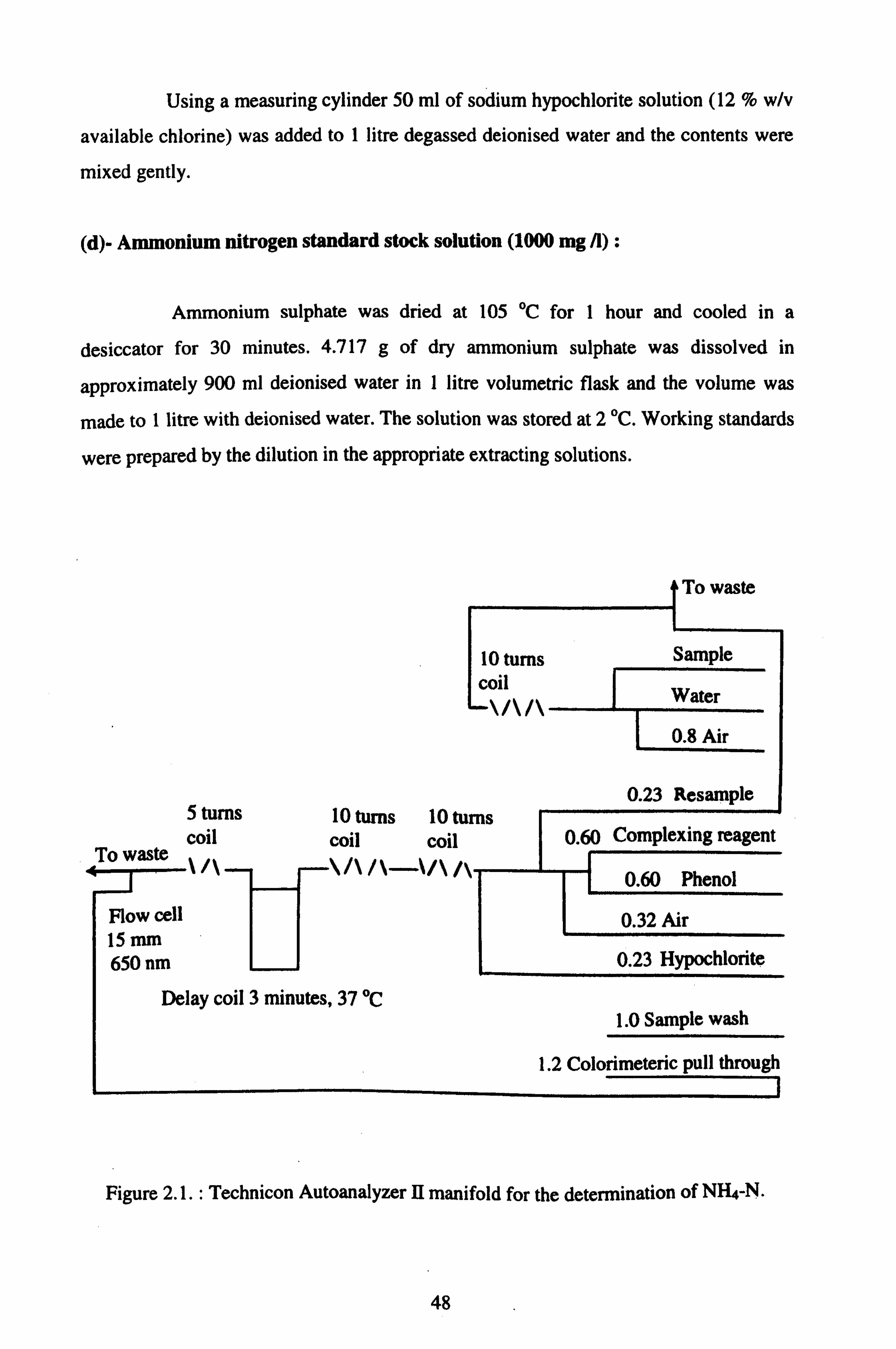
Using a measuring cylinder 50 ml of sodium hypochlorite solution (12 % w/v

available chlorine) was added to 1 litre degassed deionised water and the contents were

mixed gently.

(d)- Ammonium nitrogen standard stock solution (1000 mg /1) :

Ammonium sulphate was dried at 105 °C for 1 hour and cooled in a

desiccator for 30 minutes. 4.717 g of dry ammonium sulphate was dissolved in

approximately 900 ml deionised water in 1 litre volumetric flask and the volume was

made to I litre with deionised water. The solution was stored at 2 °C. Working standards

were prepared by the dilution in the appropriate extracting solutions.

To waste

10 turns Sample

coil Water

0.8 Air

5 turns 10 turns 10 turns coil coil coil To waste /\ /\

Flow cell 15 mm 650 nm

Delay coil 3 minutes, 37 °C

0.23 Resample T

0.60 Complexing reagent

0.60 Phenol

0.32 Air

0.23 Hypochlorite

1.0 Sample wash

1.2 Colorimeteric pull through

Figure 2.1.: Technicon Autoanalyzer II manifold for the determination of NH4-N.

48

PROCEDURE:

The manifold (Figure 2.1. ) can be used for the determination of ammonium in

water, 2M and 1M potassium chloride, 0.5 M potassium sulphate and several other

extractants. The flow rate of the standard method is shown in Table 2.1.

Table 2.1.: Reagent flow rate of the standard method for the ammonium-N determination.

Tube Flow rate (ml /min

Sample 0.23 Hypochlorite 0.23 Complexing reagent 0.60 Alkaline phenol 0.60 Air 0.32 Pull through 1.20

The solutions were analysed using the manifold shown in Figure 2.1. along

with standard solutions, blanks and zeros. The samples were run at the rate of 50 per

hour but where dilution was required the sampling rate was reduced to 40 per hour. The

colour was developed in the manifold water bath at 37 T. The colour intensity was

measured at 650 nm. The air was cleaned of atmospheric ammonia by bubbling through

5% HCl solution. The calibration graph for ammonium is linear from 0.0 to 5 mg NH4-

N A. Samples with ammonium - nitrogen concentrations higher than 5 mg/l were diluted

into the range 0.0 to 5 mg/l using an inbuilt diluter.

The standard method for ammonium nitrogen determination was developed as

described in section 3.1.2.1.

2.11.1.2. DETERMINATION OF AMMONIUM-N (TOTAL NITROGEN)

IN KJELDAHL DIGESTS

The plant material was digested by the method of Bremner and Mulvaney

(1982) as described in section 2.21. Ammonium nitrogen was determined in the

49

Kjeldahl digests by the Technicon Autoanalyzer II system as described in section 3.1.3.2. with certain modifications as follows :

ADDITIONAL REAGENTS :

In addition to the reagents used for the determination of ammonium as

described in section 3.1.3.2., the following reagents were prepared :

(a)- Wash chamber solution (5 % H2SO4) :

Carefully 50 ml of concentrated sulphuric acid was dissolved in about 800 ml deionised water, then cooled and the volume was made to 1 litre with deionised water.

(b)- Neutralising solution :

3.6 g of NaOH was dissolved in a litre of deionised water.

PREPARATION OF THE WORKING STANDARD :

(a)- Ammonium nitrogen standard stock solution (1000 mg /1) :

Dry Ammonium sulphate was dried at 105 °C for 1 hour and cooled in a desiccator for 30 minutes. 4.717 g of dry ammonium sulphate was dissolved in


made to 1 litre with deionised water. The solution was stored at 2 T. Working standards


(b)- Anunonium standard 0.0 mg /1:

5 ml of concentrated sulphuric acid and a half Kjeldahl tablet were added to a

digestion tube. Then the tube was heated to dissolve the catalyst tablet and when cooled

the contents were diluted carefully and transferred to a 100 ml volumetric flask. The

volume was made to 100 ml with deionised water.

50

(c)- Ammonium standard 100 mg /1:

5 ml of concentrated sulphuric acid and a half Kjeldahl tablet were added to a digestion tube. Then the tube was heated to dissolve the catalyst tablet and when cooled the contents were diluted carefully and transferred to a 100 ml volumetric flask. 10 ml

of 1000 mg /1 stock ammonium standard solution was added and the volume was made

up to 100 ml with deionised water.

PROCEDURE:

The filtered solutions were analysed directly on a Technicon Autoanalyzer II

system. The samples were run at the rate of 40 per hour with a dilution / neutralisation

step before the main manifold. The calibration graph for ammonium is linear from 0.0 to 100 mg NH4-N /1.

Dilution / neutralism

sample wash solution

Dilution ratio

Neutralising solution

Sample

Air

Lion step :

5% v/v H2SO4.

20 :1

2.0 ml /minute.

0.1 ml /minute.

0.8 ml /minute.

2.11.1.3. AUTOMATED DETERMINATION OF NITRATE AND NITRITE NITROGEN

In the automated system, nitrate nitrogen is quantitatively reduced to nitrite nitrogen followed by determination of the nitrite using the Greiss reagent. The method, therefore, measures nitrate plus nitrite. The nitrite nitrogen can be measured separately

on the same manifold by omitting the reduction reagents (Best, 1976). The schematic diagram of the flow system of nitrate and nitrite is shown in Figure 2.2.

51

To waste

10 turns Sample

coil Water

0.8 Air

0.32 Buffer borate 10 turns 20 turns

To waste coil coil


1.2 Colorimetric pull through

Figure 2.2.: Technicon Autoanalyzer II manifold for the determination of N03-N and N02-N.

REAGENTS:

Analar grade reagents and nitrogen free deionised water were used throughout.

These reagents were prepared in a fume cupboard. A fume cupboard was cleared and a2

figure top pan balance was set up. Care was taken to ensure that the balance was

properly locked before attempting to move it. The fan was switched off while actual

weighing was in progress but otherwise was kept running. Any spills were cleared up

immediately. When finished, the balance was wiped down and returned to the balance

bench. Finally, the fume cupboard was wiped down.

10 turns 10 turns coil coil

2 delay coils 3 minutes, 37 °C

0.42 Reducing reagent

0.42 Catalyst

solution 0.32 Air

0.16 Resample

1.0 Sample wash

0.32 Greiss reagent

52

(a)- Buffer solution :

22.5 g sodium tetraborate and 2.5 g sodium hydroxide were dissolved in 900

ml deionised water and the volume was made to I litre with deionised water. The

solution was degassed for 10 minutes in the ultrasonic bath.

(b)- Greiss reagent :

***** Concentrated hydrochloric acid is highly corrosive. Sulphanilamide is

carcinogenic and a dust hazard. Prepare this reagent in a fume cupboard. *****

Carefully 100 ml concentrated hydrochloric acid was added (measuring

cylinder) into approximately 800 ml deionised water. This solution was degassed for 10

minutes in the ultrasonic bath. Working in a fume cupboard 10.0 g sulphanilamide and

0.5 g N-1-naphthylene diamine dihydrochloride were weighed into a1 litre beaker. 500

ml of the acid solution was added carefully and the contents were stirred gently using a

magnetic stirrer. Return to the bottle, the volume was made to 1 litre with degassed

deionised water and the contents were mixed gently. The solution was stored at 2 °C.

(c)- Reducing reagent :

***** Hydrazine sulphate is a dust hazard and a suspected carcinogen.

Ensure that you are familiar with the MSDS sheet. Prepare this reagent in a fume

cupboard. *****

0.30 g of hydrazine sulphate was weighed into a small beaker. The contents

were transferred carefully to a1 litre volumetric flask containing approximately 900 ml

degassed deionised water. The volume was made up to the mark with deionised water

without shaking and the hydrazine sulphate was dissolved with a magnetic stirrer

keeping the top of the flask closed in order to prevent access of oxygen. 1 ml of 15 %

Brij. -35 solution was added and the contents were mixed gently. If the hydrazine

sulphate is shaken in a flask which is partly filled with deionised water, it will react with

the oxygen content of the flask and decrease its reducing power.

53

(d)- Catalyst solution :

1 ml 2.47 % copper sulphate solution and 1 ml 15 % Brij. -35 solution were

added to 1 litre of degassed deionised water and the contents were mixed gently.

(e)- Nitrate nitrogen standard stock solution (1000 mg /1) :

Sodium nitrate or potassium nitrate was dried at 105 °C for 1 hour and

cooled in a desiccator for 30 minutes. 6.068 g of dried sodium nitrate or 7.218 g of

dried potassium nitrate was dissolved in deionised water in 1 litre volumetric flask and

the volume was made to 1 litre with deionised water. The solution was stored at 2 T.

Working standards were prepared by the dilution in the appropriate extracting solutions.

(f)- Nitrite nitrogen standard stock solution (1000 mg /1) :

Sodium nitrite was dried at 105 °C for 1 hour and cooled in a desiccator for

30 minutes. 4.926 g of dried sodium nitrite was dissolved in deionised water in 1 litre

volumetric flask and the volume was made to 1 litre with deionised water. The solution

was stored at 2 T. Working standards were prepared by the dilution in the appropriate

extracting solutions.

PROCEDURE:

The manifold (Figure 2.2. ) can be used for the determination of nitrate and

nitrite nitrogen in water and a range of extracting solutions.

54

Table 2.2. : Reagent flow rate of the standard method for the nitrate and nitrite nitrogen determination.

Tube Flow rate (ml /min

Sample 0.16 Reducing reagent 0.42 Catalyst solution 0.42 Buffer borate 0.32 Greiss reagent 0.32 Air 0.32 Pull through 1.20

The solutions were analysed for nitrate and nitrite using the manifold shown

in Figure 2.2. along with standard solutions, blanks and zeros. The samples were run at

the rate of 50 per hour but where dilution was required the sampling rate was reduced to

40 per hour. The nitrate was reduced to nitrite by adding copper sulphate and hydrazine

sulphate solutions to the sample as it passed through the water bath set at 37 °C. The

nitrite - nitrogen was determined by a diazotization coupling reaction whereby a pink

colour was formed. The colour intensity was measured at 530 nm. Nitrate has a linear

calibration graph in the range 0.0 to 2.0 and curved calibration graph in the range 2.0 to

5.0 mg /1 N03-N. The calibration graph for nitrite is linear from 0.0 to 4.0 mg /1 N02-N.

Samples with nitrate - nitrogen concentrations higher than 5.0 mg /1 were diluted into

the range 0.0 to 5.0 mg/l using an inbuilt diluter.

For the determination of nitrite nitrogen, the reducing reagents were replaced

with nitrogen free deionised water containing 1 ml per litre of 15 % Brij. -35 solution.

2.11.2. AUTOMATED DETERMINATION OF SOIL INORGANIC

PHOSPHORUS

Technicon Autoanalyzer U was used for the determination of soil inorganic

phosphorus. The method is based on the formation of a phosphomolybdate complex

using antimony to accelerate the formation of the faintly yellow coloured product. The

coloured product is then reduced using ascorbic acid to give a more intense blue colour

which may be measured at 880 or 660 nm. The method is applicable to water samples

and a wide range of soil extract solutions and digests of plant or soil material.

55

REAGENTS:

Analar grade reagents and phosphorus free deionised water were used

throughout. These reagents were prepared in a fume cupboard. A fume cupboard was

cleared and a2 figure top pan balance was set up. Care was taken to ensure that the

balance was properly locked before attempting to move it. The fan was switched off

while actual weighing was in progress but otherwise was kept running. Any spills were

cleared up immediately. When finished, the balance was wiped down and returned to the

balance bench. Finally, the fume cupboard was wiped down.

(a)- Acid molybdate solution :

***** Ammonium molybdate and antimony potassium tartrate are toxic,

concentrated sulphuric acid is highly toxic and corrosive and can react violently with

water. This reagent should be prepared in a fume cupboard. *****

Carefully 60 ml concentrated sulphuric acid was added to approximately 700

ml deionised water in aI litre brown glass bottle and then the solution was cooled to

room temperature. 5.2 g ammonium molybdate was added and dissolved by stirring. 0.1

g antimony potassium tartrate was dissolved in approximately 50 ml deionised water in

a small beaker and this solution was added to the acid solution with mixing to avoid the

formation of a precipitate. The reagent was degassed for 10 minutes in the ultrasonic

bath and the volume was made up to I litre with degassed deionised water and the

contents were mixed gently. This reagent is stable for at least I month if stored in the

dark and can be degassed at intervals if required.

(b)- Ascorbic acid :

0.75 g ascorbic acid was dissolved in 100 ml degassed deionised water and dissolved by stirring gently on a magnetic stirrer. This reagent is unstable and must be

prepared in the day of use.

56

(c)- Dilution water :

0.0 to 1.0 mg PA range: 2 ml of aerosol - 22 wetting agent was added to 1 litre degassed deionised

water and the contents were mixed gently.

0.0 to 5.0 mg P /I range :

1 ml of aerosol - 22 wetting agent was added to I litre degassed deionised

water and the contents were mixed gently.

(d)- Phosphate-P standard stock solution (1000 mg /l) :

Potassium dihydrogen phosphate was dried at 105 °C for 1 hour and cooled

in a desiccator for 30 minutes. 4.394 g of dry potassium dihydrogen phosphate was

dissolved in approximately 900 ml deionised water in I litre volumetric flask and the

volume was made to 1 litre with deionised water. The solution was stored at 2 °C.

Working standards were prepared by the dilution in the appropriate extracting solutions.

PROCEDURE:

The manifold (Figure 2.3. ) can be used for the determination of phosphate in

water, acetic acid, acetate buffers, and several other extractants. For phosphorus

determination in sodium bicarbonate or ammonium fluoride a separate manifold is

required.

The solutions were analysed for phosphate using the manifold shown in

Figure 2.3. along with standard solutions, blanks and zeros. The samples were run at the

rate of 50 per hour but where dilution was required the sampling rate was reduced to 40

per hour. The colour was developed in the water bath at 37 T. The colour intensity was

measured at 880 nm. Phosphate has a linear calibration graph in the range 0.0 to 5.0 mg

P04 -P /1. Samples with phosphate concentrations higher than 5 mg /1 were diluted into

the range 0.0 to 5 mg /1 using an inbuilt diluter.

57

Sample dilution To waste

Debubbler

Sample

14 turns coil Water

0.8 Air

10 turns 10 turns coil coil To waste


Delay coil 3minutes, 37 °C

10 turns 10 tarns 0.16 ! 0.!! n

coil .- coil

[0.8 Wir

-\/\/\ \/\/\ 0.32 Air

0.32 Acid molybdate

0.32 Ascorbic acid

1.0 Sample wash


Figure 2.3. : Technicon Autoanalyzer II manifold for the determination of phosphate - P.

Manifold configuration for water samples :

Sample Diluent water

(ml /min) (ml /min)

0.16 0.80

0.42 0.60

0.60 0.42

Max sample P

(mg /1)

5.0

2.0

1.0

58

BACKGROUND COLOUR CORRECTION:

60 ml concentrated sulphuric acid was added carefully to approximately 700

ml deionised water in a1 litre glass bottle and then the solution was cooled to room

temperature. 1.67 g ammonium sulphate was added and dissolved by stirring. The

reagent was degassed for 10 minutes in the ultrasonic bath and the volume was made up

to 1 litre with degassed deionised water and the contents were mixed gently. This

reagent is stable for several months and can be degassed at intervals if required.

The acid molybdate solution was replaced with this reagent and the samples

were returned at the sample colorimeter settings.

2.11.3. DETERMINATION OF POTASSIUM IN SOIL AND WATER

Potassium was determined by the Flame photometer (Corning - Model : 410).

2.1 1.3.1. REAGENTS

Potassium standard stock solution (1000 mg /1) :

This is a Flame photometer standard stock solution (1000 mg K' /1). It is

manufactured by Ciba Coming Diagnostics Ltd.

Working standard solutions and concentrations :

Potassium working standard solutions were prepared by dilution of 1000 mg

K+ /1 standard stock solution with appropriate extracting solutions.

2.11.3.2. PROCEDURE

The Flame photometer was calibrated using 0.0,10,20,30,40 and 50 mg KK

/1 working standard solutions in the case of the soil samples and 0.0 to 5.0 mg K' /1

working standard solutions in the case of the water samples. The calibration graph is

curved for 0.0,10,20,30,40 and 50 mg K+ /1 working standard solutions and is linear

for 0.0 to 5.0 mg K+ /1 working standard solutions. After getting a stable readings for the

59

working standard solutions, the samples were run and their stable readings were

recorded. The calculations were made by a calibration curve program on a BBC

microcomputer.

2.11.4. DETERMINATION OF SODIUM IN WATER

Sodium was determined by the Flame photometer.

2.11.4.1. REAGENTS

Sodium standard stock solution (1000 mg /1) :

This is a Flame photometer standard stock solution (1000 mg Na+ /1). It is

manufactured by Ciba Corning Diagnostics Ltd.


Sodium working standard solutions were prepared by dilution of 1000 mg

Na' /1 standard stock solution with appropriate extracting solutions.

2.11.4.2. PROCEDURE

The Flame photometer was calibrated using 0.0 to 2.5 mg Na+ /1 working

standard solutions. The calibration graph is linear for 0.0 to 2.5 mg Na+ /1 working

standard solutions. After getting a stable readings for the working standard solutions, the

samples were run and their stable readings were recorded.

2.11.5. DETERMINATION OF CALCIUM IN SOIL AND WATER

Calcium was determined by the Atomic Absorption Spectrophotometer

(Perkin Elmer - Model : 1100 B).

60

2.11.5.1. REAGENTS

Calcium standard stock solution (1000 mg /1) :

This is a calcium nitrate standard stock solution (1000 mg Ca /1). It was

supplied by BDH Spectrosol.

Releasing agent :

SrCl2 solution was used to release calcium from the interference with

phosphate, silicate and sulphate.

A 10 % SrC12 solution or 30 % SrC12.6H20 solution was used as a releasing

agent for the determination of calcium in the soil samples. A1 .0% SrC12 solution or 3.0

% SrC12.6H20 solution was used as a releasing agent for the determination of calcium in

the water samples. This was added to standards and samples.


Calcium working standard solutions were prepared by dilution of 1000 mg Ca

/1 standard stock solution with appropriate extracting solutions and with the addition of

releasing agent.

2.11.5.2. PROCEDURE

The Atomic Absorption Spectrophotometer was calibrated using 0.0 to 5.0

mg Ca /1 working standard solutions. The calibration graph is linear for 0.0 to 5.0 mg Ca

/1 working standard solutions. After getting a stable readings for the working standard

solutions, the samples were run and their readings were recorded.

2.11.6. DETERMINATION OF MAGNESIUM IN SOIL AND WATER

Magnesium was determined by the Atomic Absorption Spectrophotometer.

61

2.11.6.1. REAGENTS

Magnesium standard stock solution (1000 mg /1) :

This is a magnesium nitrate standard stock solution (1000 mg Mg /1). It was


Releasing agent :

SrC12 solution was used to release magnesium from the interference with

phosphate, silicate and sulphate.

A 10 % SrC12 solution or 30 % SrC12.6H20 solution was used as a releasing

agent for the determination of magnesium in the soil samples. A 1.0 % SrC12 solution or

3.0 % SrC12.6H20 solution was used as a releasing agent for the determination of

magnesium in the water samples. This was added to standards and samples.


Magnesium working standard solutions were prepared by dilution of 1000 mg

Mg /1 standard stock solution with appropriate extracting solutions and with the addition

of releasing agent.

2.11.6.2. PROCEDURE


mg Mg /1 working standard solutions. The calibration graph is linear for 0.0 to 0.5 mg

Mg /1 working standard solutions. After getting a stable readings for the working

standard solutions, the samples were run and their readings were recorded.

2.12. DETERMINATION OF TOTAL METALS BY THE ATOMIC


2.12.1. DETERMINATION OF IRON IN WATER

Iron was determined by the Atomic Absorption Spectrophotometer.

62

2.12.1.1. REAGENTS

Iron standard stock solution (1000 mg /1) :

This is an iron (III) nitrate standard stock solution (1000 mg Fe /1). It was



Iron working standard solutions were prepared by dilution of 1000 mg Fe /1

standard stock solution with appropriate extracting solutions.

2.12.1.2. PROCEDURE


mg Fe /I working standard solutions. The calibration graph is linear for 0.0 to 5.0 mg Fe


solutions, the samples were run and their readings were recorded.

2.12.2. DETERMINATION OF COPPER IN SOIL

Copper was determined by the Atomic Absorption Spectrophotometer.

2.12.2.1. REAGENTS

Copper standard stock solution (1000 mg /1) :

This is copper (II) nitrate [Cu(NO3)2] standard stock solution (1000 mg Cu

/1). It was supplied by BDH Spectrosol.


Copper working standard solutions were prepared by dilution of 1000 mg Cu

/1 standard stock solution with appropriate extracting solutions.

63

2.12.2.2. PROCEDURE


mg Cu /1 working standard solutions. The calibration graph is linear for 0.0 to 5.0 mg

Cu /1 working standard solutions. After getting a stable readings for the working

standard solutions, the samples were run and their readings were recorded.

2.12.3. DETERMINATION OF NICKEL IN SOIL

Nickel was determined by the Atomic Absorption Spectrophotometer.

2.12.3.1. REAGENTS

Nickel standard stock solution (1000 mg /1) :

This is nickel nitrate [Ni(N03)2.6H201 standard stock solution (1000 mg Ni



Nickel working standard solutions were prepared by dilution of 1000 mg Ni /1


2.12.3.2. PROCEDURE


mg Ni /1 working standard solutions. The calibration graph is linear for 0.0 to 2.0 mg Ni


solutions, the samples were run and their readings were recorded

2.12.4. DETERMINATION OF ZINC IN SOIL

Zinc was determined by the Atomic Absorption Spectrophotometer.

64

2.12.4.1. REAGENTS

Zinc standard stock solution (1000 mg /1) :

This is zinc nitrate [Zn(N03)2.4H20] standard stock solution (1000 mg Zn



Zinc working standard solutions were prepared by dilution of 1000 mg Zn /1


2.12.4.2. PROCEDURE


mg Zn /1 working standard solutions. The calibration graph is linear for 0.0 to 1.0 mg Zn

q working standard solutions. After getting a stable readings for the working standard


2.12.5. DETERMINATION OF CHROMIUM IN SOIL

Chromium was determined by the Atomic Absorption Spectrophotometer.

2.12.5.1. REAGENTS

Chromium standard stock solution (1000 mg /1) :

This is chromium (111) nitrate standard stock solution (1000 mg Cr /1). It was



Chromium working standard solutions were prepared by dilution of 1000

mg Cr /1 standard stock solution with appropriate extracting solutions.

65

2.12.5.2. PROCEDURE


mg Cr /1 working standard solutions. The calibration graph is linear for 0.0 to 5.0 mg Cr

/I working standard solutions. After getting a stable readings for the working standard


2.12.6. DETERMINATION OF CADMIUM IN SOIL

Cadmium was determined by the Atomic Absorption Spectrophotometer.

2.12.6.1. REAGENTS

Chromium standard stock solution (1000 mg /1) :

This is cadmium nitrate [Cd(N03)2.4H20] standard stock solution (1000 mg

Cd /1). It was supplied by BDH Spectrosol.


Cadmium working standard solutions were prepared by dilution of 1000 mg

Cd /1 standard stock solution with appropriate extracting solutions.

2.12.6.2. PROCEDURE


mg Cd /1 working standard solutions. The calibration graph is linear for 0.0 to 2.0 mg

Cd /1 working standard solutions. After getting a stable readings for the working

standard solutions, the samples were run and their readings were recorded

2.12.7. DETERMINATION OF LEAD IN SOIL

Lead was determined by the Atomic Absorption Spectrophotometer.

66

2.12.7.1. REAGENTS

Lead standard stock solution (1000 mg /1) :

This is lead nitrate [Pb(NO3)2] standard stock solution (1000 mg Pb /1). It

was supplied by BDH Spectrosol.


Lead working standard solutions were prepared by dilution of 1000 mg Pb /1


2.12.7.2. PROCEDURE

The Atomic Absorption Spectrophotometer was calibrated using 0.0 to 20

mg Pb /1 working standard solutions. The calibration graph is linear for 0.0 to 20 mg Pb



2.13. FLAME CONDITIONS OF ANALYSIS BY THE ATOMIC ABSORPTION

SPECTROPHOTOMETER

Table 2.3.: Flame conditions of analysis of calcium, magnesium and iron.

Flame conditions Ca M Fe

Wavelength (nm) 324.8 285.2 248.3 Lamp current 10.0 6.0 30.0 Fuel Flow (C2H2) 2.5 2.5 2.5 Air flow 8.0 8.0 8.0 Background correction Off On On

67

Table 2.4. : Flame conditions of analysis of cadmium, chromium, copper, nickel, zinc and lead.

Flame conditions

Cd Cr Cu Ni Zn Pb

Wavelength (nm) 228.8 357.9 324.8 232.0 213.9 283.3 Lamp current 8.0 12.0 10.0 30.0 10.0 15.0 Fuel Flow (C2H2) 2.5 3.5 2.5 2.5 2.5 2.5 Air flow 8.0 8.0 8.0 8.0 8.0 8.0 Background On Off Off On On On correction

2.14. ANALYSIS OF METALS BY THE INDUCTIVELY COUPLED PLASMA

SPECTROSCOPY

Chromium, cadmium, nickel, zinc, lead, copper, boron, barium, manganese,

magnesium and potassium were determined by the Inductively Coupled Plasma Optical

Emission Spectroscopy (ICP-OES) using a Thermounicam IRIS Radial ICP/CID. The

analysis preferences are presented in Table 2.5. The plasma conditions are shown in

Table 2.6. The analysis conditions of chromium, cadmium, nickel, zinc, lead, copper, boron, barium, manganese, magnesium and potassium are given in Table 2.7.

Table 2.5.: The analysis preferences.

Analysis references

Number of repeats 3.0 Delay time (sec) 0.0 Sample flush time (sec) 60.0 Integration time : Low wavelength range (sec) 30.0 High wavelength range (sec) 5.0

68

Table 2.6.: The plasma conditions.

Plasma Conditions

Auxiliary gas Low RF power 1150 Nebulizer pressure (PSI) 32 Flush pump rate (rpm) 100 Analysis pump rate (rpm) 100 Relaxation time (sec) 0.0

Table 2.7. : The analysis conditions of chromium, cadmium, nickel, zinc, lead, copper, boron, barium, manganese, magnesium and potassium.

Analysis Cd Cr Ni Zn Pb Cu conditions

Wavelength (nm) 226.502 283.563 231.604 213.856 220.353 327.396 (order) (116) (93) (114) (123) (119) (80)

Subarray information :

Subarray width 15 15 15 15 15 15 Subarray height 3 3 3 3 3 3 Centre width 1 2 1 1 2 1

Background position :

Left position* 1 1 1 1 1 1 Right position* 12 15 15 15 15 15

Standard 10 mg /1 10 mg /1 10 mg /1 10 mg /1 10 mg /1 10 mg /1 concentration All All All All All All

QC Check 5.0 mg /1 5.0 mg /1 5.0 mg 5.0 mg /1 5.0 mg /1 5.0 mg /1 All All All All All All

* All background width = 1.

69

Table 2.7. : Continued.

Analysis B Ba Mn Mg K conditions

Wavelength (nm) 249.773 233.527 259.373 285.213 769.896 (order) (105) (113) (101) (92) (34)

Subarray information : 15 15 15 15 15

Subarray width 3 3 3 3 3 Subarray height 1 2 2 2 1 Centre width

Background position : 1 1 1 1 5

Left position* 15 13 15 15 15 Right osition*

Standard concentration 10 mg /I 10 mg /l 10 mg /1 10 mg /1 10 mg /1 All All All All All

QC Check 5.0 mg /1 5.0 mg /1 5.0 mg /1 5.0 mg /1 5.0 mg /1 All All All All All

2.15. DETERMINATION OF ANIONS BY ION CHROMATOGRAPHY

Fluoride, nitrite, nitrate, chloride, bromide, sulphate and phosphate were

determined in the filtrate by Ion Chromatography (Model : DIONEX DX 500 Ion

Chromatography System).

The system consisted of :

1- GP40 Gradient Pump.

2- LC10 Chromatography Module (AGI 1 Guard Column and AS 11 Separator Column

and ASRS Anion Self Regenerating Suppresser).

3- ED40 Electrochemical Detector.

4- Computer running Peak Net Chromatography Software (version 4.3).

70

METHOD OF SEPARATION :

The seven anions were separated by gradient separation. The gradient

separation is shown in Table 2.8.

Table 2.8. : The gradient separation.

Time (minutes Water 200 mM NaOH

0.0, 97.5% 2.5% 1.0 97.5% 2.5%

10.0 85.0% 15.0% 10.1 97.5% 2.5% 15.0 97.5 % 2.5 %

METHOD PARAMETERS :

Eluent flow rate = 2.0 ml /min.

Injection loop = 25.0 µl.

Detector Mode = Conductivity.

SRS current .= 300 mA.

The retention time and standard calibration details are shown in Table 2.9.

Table 2.9.: The retention time and standard calibration details.

Component Retention time Standard concentration

Fluoride 0.96 1.0 mg /1 Chloride 1.70 1.0 mg /1 Nitrite 2.01 1.0 mg /I Bromide 3.23 1.0 mg /1 Nitrate 3.36 1.0 mg /1 Sulphate 4.62 1.0 mg /1 Phosphate 7.72 1.0 mg /1

71

2.16. DETERMINATION OF CATION EXCHANGE CAPACITY IN SOIL

Negative charges on the clay and organic matter in soils provide sites at

which cations can be held by ion exchange. Nutrients held in this way are considered to

be available to plants. Thus a measure of both the total amount of negative charge and

the percentage holding nutrient cations will give information regarding the potential and

actual fertility of a soil.

The measurement of cation exchange capacity gives the total quantity of

negative charge in a soil, and so indicates the soil's ability to hold cations. The cation

exchange capacity is made up of :

(a)- Fixed charge on the clays to imperfections in the crystal lattice (isomorphous

substitution).

(b)- pH dependent charges on clay edges and organic matter. Therefore, it is important to state at what pH the cation exchange capacity is

measured. The method described below involves saturation of the negative sites with K+

ions at pH 7.0. As other methods use different saturating (or index) cations, it is also

important to state which index ion is being used.

The negative charges were measured with K+ ions by leaching the soil with

an excess of potassium, so removing other exchangeable cations by mass action. The

excess K+ ions were then removed with 95 % ethanol and K+ hold on the negative sites

were displaced by leaching the soil with NH4' ions. The solution containing the

displaced K+ ions was then made to a known volume and the concentration of K+ was

determined by flame emission using a Flame photometer.

2.16.1. PROCEDURE

Triplicate samples of 10 g air-dried less than 2 mm sieved soil were weighed

out accurately in 100 ml beaker. The soil was mixed thoroughly with 2 volumes of acid-

washed sand to assist percolation. A glass column with small pieces of glass wool were

plugged in the bottom, 1 cm depth of acid-washed sand was placed on the top of the

glass wool and the soil/sand mixtures was placed on the top of the acid-washed sand in

72

the columns. Then another half cm depth of acid-washed sand was placed on the top of

the soil/sand mixtures.

Deionised water was poured in the column to get a saturated soil and then

the leachate of deionised water was discarded. Each column was leached with 200 ml of

1M potassium acetate at pH 7.0 and then the leachate was discarded. Excess potassium

acetate was removed by leaching each column with 200 ml 95 % ethanol and then the

leachate was discarded. The column was washed from outside by deionised water, then

wiped by a tissue paper to remove any spillage of potassium acetate.

Each column was leached with 200 ml of 1M ammonium acetate at pH 7.0

and the leachate was collected in 250 ml volumetric flask. When all the ammonium

acetate had leached through the column the flask was made up to the mark with

deionised water and mixed well.

Dilution of this solution was made by a factor of 1: 100. Potassium was determined in the diluted leachate by the Flame photometer as described in section

2.11.3. using a standard series 0.0,10,20,30,40 and 50 mg K+/1 in 0.01 M ammonium

acetate solution. If necessary, the samples were diluted again as appropriate to fit in the

calibration graph and the ammonium acetate solution was maintained at 0.2 M.

If the analysis can not carried out immediately, the solution was stored in

polythene bottles in order to avoid contamination of potassium from the glass.

* Notes

1- When running this column, do not allow the soil to stand in potassium acetate over a

long period.

2- Never allow the column to run dry, except at the end of the ammonium acetate leach.

2.16.2. CALCULATION OF CATION EXCHANGE CAPACITY

The concentration of potassium in solution was measured in mg A. Cation

exchange capacity was quoted in units of c mole, /kg. This was because the

concentration of a cation was being used as a measure of negative charge :

73

Using the measured potassium concentration in mg /1, cation exchange

capacity was calculated as follows :

Weight of K+ extracted (mg) =

Concentration of K+ (mg /1) x Dilution factor x Volume of leachate (1)

c moler of K+ /kg soil =

Weight of K+ extracted (mg)

--------------------------------------------------------------------------------------- Atomic weight of potassium x 10 x weight of oven dried soil (kg)

Where :

Atomic weight of potassium = 39.1

c moles /kg is equivalent to meq. /100g.

2.17. EXTRACTION OF INORGANIC NITROGEN FROM SOIL

2.17.1. REAGENTS

PREPARATION OF 0.5 M POTASSIUM SULPHATE SOLUTION :

This solution was prepared according to Khan (1987) as follows :

Analar grade potassium sulphate reagent was used. 87.12 g potassium

sulphate was dissolved in about 800 ml deionised water in 1.5 litre beaker and the

volume was made up to 1 litre with deionised water. The solution was purified of

ammonium nitrogen contamination by first raising the pH to 11.0 with 1M potassium

hydroxide. It was then boiled and stirred for a period of 15 minutes to give off the

ammonia gas. The solution was allowed to cool and the pH was readjusted to pH 6.0

with 0.5 M sulphuric acid. Then the contents were transferred to a1 litre volumetric

flask with deionised water and the volume was made up to the mark with deionised

water. As there is no simple . method for removal of nitrate nitrogen from the

extracting solution, the potassium sulphate was first tested and a batch number with a

low level of nitrate impurities was selected for use.

74

2.17.2. EXTRACTION PROCEDURE

2.5 g fresh soil passed through a2 mm sieve was weighed in duplicate, into

a 100 ml glass bottle. 50 ml of 0.5 M K2S04 solution was added. Then the bottle was

shaken for 2 hours in a shaker in the cold room at 2 °C. The shaken samples were

filtered through Whatman No. 2 filter paper [filter paper pre washed with 0.5 M H2SO4

solution according to Shah method (1988) as described in section 2.2. ] and the filtrate

was collected in a 100 ml plastic bottle. NH4-N, N01-N and N02-N were determined in

the filtrate. The blank determination was carried out without soil.

2.18. EXTRACTION OF PHOSPHATE FROM SOIL

The extraction of phosphorus from soil was carried out according to MAFF

/ADAS method No. 59 (1986).

2.18.1. REAGENTS

PREPARATION OF 0.5 M SODIUM BICARBONATE SOLUTION :

210 g NaHCO3 was dissolved with deionised water in a 400 ml beaker.

Then the contents were transferred with deionised water to a5 litres conical flask. 25 ml

of 0.05 % m/v polyacrylamide solution was added. The volume was made up to the

mark with deionised water. Then drops of 3M NaOH solution was added until the pH,

measured with a pH meter (Mettler - Model : Delta 320), is 8.5 at 20 °C. Before use the

pH meter was standardised with the pH 7.0 and pH 4.0 buffer solutions instead of

buffer solution of pH 8.5. The pH of the reagent was checked on the day of use.

PREPARATION OF POLYACRYLAMIDE SOLUTION, 0.05 % m/v :

0.5 g polyacrylamide was dissolved in approximately 600 ml of deionised

water by stirring for several hours. The contents were left overnight to make sure it is

dissolved. When the polymer was dissolved, the contents were diluted to I litre with

deionised water.

75

PREPARATION OF 2.5 N H2SO4 SOLUTION :

69.0 ml of concentrated H2SO4 was diluted in approximately 800 ml

deionised water in a1 litre volumetric flask. Then the volume was made up to the mark

with deionised water.


2.5 g air dried soil passed through a2 mm sieve was weighed, in duplicate,

into a 100 ml glass bottle. 50 ml 0.5 M NaHCO3 solution was added. The bottle was

shaken in the end - over - end shaker at 20 °C for 30 minutes. The shaken samples were

filtered through a Whatman No. 2 filter paper and the filtrate was collected in a 100 ml

plastic bottle. Phosphorus was measured in the filtrate. The blank determination was

carried out without soil.

2.18.3. NEUTRALISATION PROCEDURE

Sodium bicarbonate soil extracts were neutralised as follows : 5.0 ml soil extract was placed into a 15 ml glass bottle. 2.0 ml of 2.5 N

H2S04 solution was added gradually. Then the glass bottle was closed by a plastic

stopper and the contents were shaken well. The stopper was taken away and the glass

bottle was left for 30 minutes for neutralisation and evolution of CO2 and then the

contents were shaken well again to make sure that all CO2 gas disappeared. Phosphorus

was determined in the neutralised extracts.

2.19. EXTRACTION OF POTASSIUM AND MAGNESIUM FROM SOIL

The extraction of potassium and magnesium from soil was carried out

according to MAFF /ADAS methods No. 40 and 63 (1986).

76

2.19.1. REAGENTS

PREPARATION OF 1M NH4NO3 SOLUTION :

80.0 g ammonium nitrate was dissolved with deionised water in a 600 ml

beaker. Then the contents were transferred with deionised water to aI litre volumetric

flask and the volume was made up to the mark with deionised water.


5.0 g air dried soil passed through a2 mm sieve was weighed, in duplicate,

into a 100 ml glass bottle. 50 ml of IM NH4NO3 solution was added. The bottle was

shaken for 30 minutes in the end - over - end shaker. The shaken samples were filtered

through a Whatman No. 1 filter paper and the filtrate was collected in a 100 ml plastic

bottle. Potassium was measured in the filtrate by the Flame photometer as described in

section 2.11.3. Magnesium was measured in the filtrate by the Atomic Absorption

Spectrophotometer as described in section 2.11.6. The blank determination was carried

out without soil.

2.20. ACID DIGESTION OF SOIL

Digestion of soil was done using a3: 1 Hydrochloric acid / Nitric acid

mixture known as Aqua Regia.

APPARATUS:

Tecator 40 tube block digester and Technicon Autoanalyzer system.

PREPARATION OF AQUA REGIA SOLUTION :

The solution contains three parts 6M HCl to one part 69 % HNO3 as follows :

300 ml of concentrated HCl + 200 ml of concentrated HNO3 + 300 ml

deionised water.

77

Where : The concentration of the concentrated HCl is 12 M.

DIGESTION PROCEDURE :

2.5 g ground soil was weighed exactly using a four figure balance, in

duplicate. Each sample was placed in a block digestion tube and 10 ml of Aqua Regia

solution was added. The tubes were allowed to stand for at least twelve hours to allow

the acid to equilibrate with the soil. The tubes were then placed in the digestion block

and the temperature was set at 125 °C. The extraction unit was switched on to remove

the brown NO2 gas evolved during the digestion. The digestion block was run for at

least 3 hours, until the tubes were clear of the brown gas. The tubes were allowed to

cool and 10 ml of deionised water was added, then the digests were filtered, with

washings using deionised water, through Whatman No. 50 hardened filter papers into 50

ml volumetric flasks. The solutions were then made up to volume using deionised water.

The solutions were transferred to a 100 ml plastic bottles for measurement. The blank

determination was carried out without soil.

2.21. TOTAL NITROGEN IN PLANT MATERIAL

The total nitrogen in plant material is determined according to the method of

Bremner and Mulvaney (1982). This method does not include oxidised forms of

nitrogen such as nitrate. Samples were digested in concentrated sulphuric acid using potassium

sulphate to raise the boiling point and a copper selenium catalyst mixture to accelerate

the digestion process. Ammonium in the digests was determined using an automated

colorimetric method on the Technicon Autoanalyzer system.

APPARATUS:

Tecator 40 tube block digester and Technicon Autoanalyzer system

78

SAMPLE PREPARATION :

The vegetation samples were oven dried and finely ground using a mill.

DIGESTION PROCESS :

REAGENTS:

Analar grade reagents and nitrogen free deionised water were used


cleared before starting. Any spills were cleared up immediately and the fume cupboard

was wiped down when finished.

Concentrated sulphuric acid (Analytical Reagent) :

***** Concentrated sulphuric acid is extremely corrosive. *****

A1 litre bottle with a5 ml dispenser was set up. The bottle was filled

carefully with analytical grade concentrated sulphuric acid. Care was taken to ensure

that the dispenser contained no air bubbles or the dispenser might spit when used. In

addition, care was taken to ensure that the dispenser did not allow acid to siphon out of

the bottle.

Kjeldahl tablets (Thompson and Capper Ltd. ) :

***** Selenium is toxic by ingestion and inhalation. It is a cumulative

poison. It is an animal carcinogen and there is evidence of reproductive effects. OES =

0.2 mg /m3. *****

These tablets contained :

100 parts potassium sulphate (K2SO4), 6 parts copper (II) sulphate

(CuSO4.5H20) and 1 part selenium (Se).

The 5g tablet was split in half.

***** Take care handling the catalyst tablets which contain selenium. Wear

gloves. This operation must be carried out in a fume cupboard. *****

79

PROCEDURE:

0.2 g plant material (maximum 10 mg N) was weighed carefully to the

nearest 0.1 mg approximately into a digestion tube. Care was taken to ensure that all the

sample reached the bottom of the tube. This can be done using a foil weighing boat with

a long detachable handle and by ensuring that the tube is carefully dried. The boat was

tarred and the required amount of sample was added. This weight was recorded.

Handling the weighing boat with forceps, the handle was attached to the weighing boat;

and holding the digestion tube horizontally, the sample was passed to the base of the

digestion tube. Using forceps, the weighing boat was removed from the handle, weighed

and the weight was recorded. The difference in weight is the weight of sample

transferred to the digestion tube.

Half catalyst tablet was added to each digestion tube.

***** Take care handling the catalyst tablets which contain selenium. Wear

gloves. This operation must be carried out in a fume cupboard. *****

Using a dispenser, 5.0 ml (± 0.1 ml) concentrated sulphuric acid was added. ***** Take care handling the concentrated sulphuric acid as it is highly

corrosive. Ensure that the dispenser contains no air bubbles or the dispenser may spit

when used. Ensure that the dispenser does not allow acid to siphon out of the bottle.

Point both the dispenser nozzle and the tube away from the body when dispensing the

acid. Wear acid resistant gloves. This operation must be carried out in a fume

cupboard. *****

The tubes were left for 15 minutes to soak the concentrated sulphuric acid

so as to provide wet plant material. ***** The digestion block should be set up in a fume cupboard along with

its own fume extraction system and the fume cupboard set on high. *****

The rack of tubes was placed in the digestion block and the fume extraction

system was set up. The heating was gently at first until the initial frothing subsided.

Plant digests are likely to froth severely in the initial stages if the initial heating is too

vigorous. Once the initial carbonisation was complete, the temperature was increased to

375 °C and heating was continued until the digests clear. The baffle was placed on the

front of the rack to promote refluxing higher up the tubes thereby washing material

down into the tubes.

80

Once this was complete, the baffle was removed to prevent excessive loss

and heating was continued for 1 hour.

The tubes were removed from the block and allowed to cool until just

warm to the touch. If left too long, the digests may solidify and become very difficult to

dissolve. Very carefully and pointing the tube towards the back of the fume cupboard,

about 10 ml deionised water was added from a wash bottle.

***** The reaction on adding water to the concentrated sulphuric acid

will be very vigorous and if the digests are too warm the acid may spurt from the end of

the tube. *****

Once all the tubes have been diluted, a further 30 ml deionised water was

added and mixed well. The contents were filtered through a Whatman No. 1 filter paper

into 100 ml volumetric flasks. The tube was washed at least twice and these washings

were added to the filter paper. Do not use hardened grades of filter paper as these may

contain high levels of nitrogen. The volumetric flask was made up to the mark with

deionised water, stoppered and mixed well. The blank determination was carried out

without soil.

81

CHAPTER 3

METHODS DEVELOPMENT AND ASSESSMENT

3.1. AMMONIUM ANALYSIS IN SOIL AND WATER

3.1.1. INTRODUCTION

The current methods for measuring ammonium in aqueous solutions include

steam distillation, microdiffusion, ion selective electrodes, fluorometric and

colorimetric.

Willason and Johnson (1986) illustrated a reliable and sensitive gas diffusion

technique for the rapid determination of ammonia in seawater based on the colour

change in a pH indicator solution. They showed that the procedure is based on the

conversion of NH4-N in seawater to NH3 and that following diffusion of NH3 through a

hydrophobic membrane using flow - injection analysis. The change in light

transimittance of the acceptor stream produced by the ammonia due the change in the

pH is measured by a light - emitting diode (LED) photometer. The magnitude of the

change in the colour is proportional to the concentration of ammonia in the sample. The

sampling rate of 60 samples per hour can be made on a flowing stream of seawater or

discrete samples. In addition, the lower limit of detection is 0.7 µg A. The method is

ideal for mapping ammonia concentrations in estuarine, coastal and oceanic waters since

it is very sensitive and automated (one sample per minute).

Aoki et al. (1986) suggested a new continuous flow method for the

simultaneous determination of nitrate and ammonia in water. They reported that

ammonia is fluorometrically determined with an o-phthalaldehyde reagent followed by

the reduction of nitrate to ammonia in alkaline medium by titanium (III) chloride to

determine nitrate. The separation of the ammonia generated in the alkaline sample

solution is carried out with a tubular microporous PTFE membrane. Although nitrite

stoichiometrically interferes but can be controlled by sulfanilic acid. Satisfactory results

were obtained for the simultaneous determination of nitrate and ammonia in rivers. The

limits of detection (3 standard deviations) for nitrate and ammonia were 25.2 x 10-4 and

82

25.2 x 10"5 mg /1, respectively. The method is so sensitive to nitrate that it gave a

satisfactory result even in the case of the Uji River where the indirect photometric

chromatography method failed because of insufficient sensitivity.

The colorimetric methods include the Berthelot and the Nesseler methods.

These two methods have both been used in manual and automated colorimetric

methods. Automated methods have the greatest accuracy and precision (Brown, 1973).

In addition, since large numbers of samples can be analysed quickly and with a high

degree of reproducibility, automated analysis for the determination of the inorganic

nutrients in water and various soil extracting solutions is an attractive alternative to

manual wet chemistry procedures (White and Gosz, 1981; and Burton et al., 1989).

The most commonly used automated technique for measuring ammonium

concentration is the indophenol blue method (Berthelot method).

Searle (1984) produced a large review about the Berthelot reaction. He

indicated that the so called Berthelot reaction (sometimes called the indophenol

reaction) is the reaction of ammonium ions and a phenol, which results in the formation

of an indophenol dye under suitable oxidising conditions in the presence of

hypochlorite. The strong absorbance of the indophenol dyes lies between 630 and 720

nm since they are highly conjugated. Based on this reaction there are sensitive methods

specific for the ammonium ion. These methods can also be applied to the methods in

which nitrogen is converted into the ammonium form by suitable pre - treatments, such

as Kjeldahl digestion. The complexity of the reaction mechanism caused problem in the

early manual methods. Considerable interest in the reaction has stemmed almost entirely

from the development of automated analysis, particularly continuous flow analysis

(CFA) in which the reaction conditions are controllable and reproducible. Use of the

automated Berthelot reaction became widespread where there are large numbers of

samples for nitrogen determination. The popularity of the automated method is also

because the reaction conditions are closely controlled. The most commonly used

automated version of the Berthelot reaction is the nitroprusside catalysed reaction since

it has high sensitivity and it reaches equilibria faster than the uncatalysed reaction. As

the published automated methods are based on aqueous chemistry the phenolic

compounds used are either phenol or salicylic acid because of the solubilities of their

respective sodium salts. Although early workers recognised that other phenol

83

compounds could be used in the reaction, phenol has been the most widely used

phenolic compound . These phenolic compounds include thymol, salicylic acid and its

salts, a-naphthol, guaiacol, o-phenylphenol, o-chlorophenol, 2-methyl-5-

hydroxyquinoline and m-cresol. Although phenol is cheap and readily available, it is,

however, toxic by skin absorption. Phenol should be used with care since it is

associated with handling hazards (poisonous, volatile) and the formation of a very

unpleasantly smelling compound during the reaction. Because its solubility, low toxicity

and high convenience to prepare sodium salicylate is also popular.

Although causing a rapid fading in the colour intensity with time, a development temperature of 100 °C was often used and maximum colour development

occurred relatively rapidly in some of the early uncatalysed methods using phenol and

hypochlorite reagents (Searle, 1984). A number of reagents have been used as catalysts

for this reaction , including sodium nitrosylpentacyanoferrate (II) (sodium

nitroprusside), acetone, potassium hexacyanoferrate (II) and sodium

aquopentacyanoferrate (II) (Krom, 1980). Sodium nitroprusside has been established as

the best catalyst for the reaction providing the greatest sensitivity (Searle, 1984).

The achievement of the formation of monochloroamine as the first stage in

the reaction mechanism is obtained in the presence of hypochlorite, although the

reaction proceeds through a similar mechanism when the hypochlorite is substituted, for

example by organochlorine salts. The common source of hypochlorite ions is sodium

hypochlorite (Searle, 1984). A number of reagents have been used as a source of

hypochiorite ion, including sodium hypochlorite, sodium dichloroisocyanurate (NaDTT)

and chloramine - T. Because of the stability of sodium dichloroisocyanurate a known

concentration of chlorine can be provided for the reaction without the need for frequent

standardisation, which is necessary if sodium hypochlorite is used (Krom, 1980).

However, the rate of hydrolysis of these compounds to hypochlorite may depend on the

reaction conditions. In addition, sodium hypobromite can be used. Although sodium

hypochlorite is the most widely used source of hypochlorite ion, there is increasing use

of organochlorine salts such as sodium dicloroisocyanurate.

Interference problems in the Berthelot reaction for nitrogen determination in

ecological materials, are most likely to occur with soil samples (Rowland, 1983). When

nitrogen groups such as amino, amide or amine hydrolyse to ammonia under the

reaction conditions, positive interferences can arise. Interference also occurs in the

84

reaction in the presence of sufficient amount of some metals e. g. copper and mercury.

Among the non metallic elements which cause interference are sulphur in a range of

oxidation states, selenium and the halogens. The tendency of high salinity samples such

as seawater to lower the reaction pH is considered to result from the precipitation of

insoluble hydroxides (Searle, 1984). Furthermore, the precipitation as hydroxides at the

pH of the reaction occurs due to some elements commonly found in soil extracts such as

Ca, Mg, Fe and other divalent and trivalent cations. This may cause a noisy signal and

results in erratic readings. Potassium sodium tartrate, trisodium citrate . and EDTA have

been used to eliminate the interference and prevent the precipitate from forming (Gentry

and Willis, 1988).

O'Donovan (1971) found that tris (hydroxymethyl) methylamine (Tris),

glutamine and phosphate inhibited the development of the indophenol colour formed by

ammonia, phenol and hypochlorite, however, these compounds did not change the

indophenol colour after its development.

Searcy et al. (1965) assessed the Berthelot colour reaction and showed that

the sequence of adding reagents is an important parameter in the chromogenic response.

The critical factor is the time lapse before the addition of the phenol reagent to the

alkaline hypochiorite - containing mixtures. The volatilisation of ammonia from

solutions treated with alkaline hypochlorite occurs because of the high pH. The

prevention of this loss can be accomplished by adding the phenol reagent before the

alkaline hypochlorite. It appears that the specificity of Berthelot colour formation can

be enhanced by the phenol - hypochlorite reagent sequence.

Weatherburn (1967) examined the Berthelot colour reaction with the

particular aim of presenting a simple, reliable analytical procedure. Excellent

reproducibility with great convenience was obtained by using the combination of two

reagents prepared readily ( phenol plus nitroprusside and alkali plus hypochlorite). The

hypochlorite reagent could be added up to 30 minutes after the mixing of the ammonium

containing sample with the phenol reagent without change of absorbance, however, the

mixing of the sample with a reagent containing hypochiorite or with alkaline phenol

plus nitroprusside lead to a decrease in absorbance unless the second reagent was added

immediately. The complicated interrelationship between reaction temperature,

development time and nitroprusside concentration in the nitroprusside catalysed reaction

makes comparisons between methods difficult, as a considerable range of nitroprusside

85

concentrations are used. The development of colour was satisfactory with minimal

precautions as a result of using a variety of reagent concentrations and reaction

temperatures of 20,25,37 and 75 °C. At 37 °C the development of colour was faster

than at the room temperature ( 15 - 25 °C). Although the time to reach maximum

absorbance was longer than at 37 °C, there was an increase in the sensitivity at 75 °C.

The absorbance maximum was reached quickly at 100 °C, however, this temperature

was not recommended because of the rapid decrease in the absorbance thereafter. As the

absorbance reached a maximum rapidly and decreased abruptly, a reaction temperature

of 100 °C would require critical timing and rigid duplication of standards . It is not

desirable to use a temperature of 50 °C for the reaction because of the slight but

continuing increase in absorbance with most concentrations of nitroprusside

Searle (1975) discussed an automated method for the measurement of

ammonium ions in Kjeldahl digests and IM sodium chloride extracts of soils (for the

determination of total nitrogen and cation exchange capacity, respectively). Based on the

nitroprusside catalysed indophenol reaction, and using a Technicon Autoanalyzer II the

analysis rates of 100 per hour were possible. There was a good agreement between the

method and the standard distillation - titration method. Although the maximum colour

development for the indophenol reaction occurred between pH 10 - 13, reaction

conditions approaching pH 14 were used in order to have sufficient alkali present to

neutralise the acid Kjeldahl digests. The accuracy of the Autoanalyzer method

described, over the range 0- 70 mg /1 N, provided linear calibration over this range as

well as it was capable of high analysis rates.

Verdouw et al. (1977) developed an ammonia determination method based

on the formation of a substituted indophenol with sodium salicylate as the phenolic

reagent . They reported that the salicylate method is used specifically for NH3-N and in

natural fresh water samples, interferences are generally absent, also the method can be

easily applied for sea water analysis. Compared with the phenol method, salicylate is a

good alternative for phenol. Although the low reactivity of the salicylate as a result of

the introduction of a carboxylgroup (salicylate concentration is 4 times the phenol

concentration for optimal conditions), the disadvantages of phenol, i. e. volatile reagent

and o-chlorophenol formation, are much reduced, however, the sensitivity was

negligibly decreased. It seems that the salicylate method has proved to be very useful

since its ease in application and great reproducibility.

86

Krom (1980) suggested a reaction scheme (Figure 3.1. ) for the

spectrophotometric determination of ammonia by using a modified Berthelot reaction, in

which salicylate, dichloroisocyanurate and complex cyanides are the principal reagents.

He pointed out the first action of the complex cyanides in the reaction was to stabilise

monochloramine at pH values (12 - 13) at which it is normally unstable and hence

facilitate the formation of 5-aminosalicylate from salicylate (this step is the rate

determining step of the reaction), and the second action was to accelerate the oxidative

coupling of 5-aminosalicylate with salicylate to form the indophenol dye [possibly via a

hexacyanoferrate (III) intermediate]. The necessity to optimise the pH value for each

combination of reagents used is opened up since the optimum pH of reaction is a result

of a complex inter - relationship of a number of equlibria. Since the A.,,, , was 650 - 660

nm for all combinations of reactants the differences in the absorbencies could not have

been related to measurement at a wavelength considerably different from A. ..

Rowland (1983) used the Berthelot reaction as an Autoanalyzer method for

the analysis of ammonium - nitrogen. He stated that this method has a wide versatility as

it can be applicable for the determination of total nitrogen in soils and plant material,

and sufficiently is stable and sensitive to determine levels of NH4-N in natural waters.

The interference of amino acids contributed a relatively small fraction (11 %) in soil

extracts and was not present in the soil solution examined. The use of disodium

hydrogen phosphate buffer enhanced the interference from amino acids and precipitated

calcium phosphate from calcareous soil extracts.

87

Hydr*ds of-dibocy t

CyCI= " HCyO- ý-= Cya H20-º

HCY2' C

* NOCI I" HOCI

wMr. Cy Is -N -

ec--4! %o

Monochioramins fornUtI n

NH3 + HOCI NHP + H2O (2)

H ON

C00' O+ NHIO* --ý O 13)

NH2

5-Aminoss icylate

OH

I COO Oxt

COO'

NH= NH

0" 0 coo

61" +

C00' COO- OxkbtiOst eouplinq N 16)

NH

COO' 0

IP dye

Figure 3.1.: Reaction sequence according to Krom (1980).

III

Markus et al. (1985) introduced the automated procedures for determining

N02-N, N03-N and NH4-N in various soil testing programs using an Autoanalyzer

system equipped with a microprocessor - based controller and data handler. They

reported that the new system provides improvement in accuracy and precision of results

through its drift, gain, and carryover correction features. Furthermore, the new system

also potentially offered a more rapid chemical determination. The determination of NO3-

N and NH4-N in standard solutions gave a very high degree of accuracy at each of the

60,90 and 120 per hour sampling rates studied. The variations in analytical results and

the evaluated precision indicate the diminution in quality of both N03-N and NH4-N

88

analyses at the 120 per hour sampling rate. A very close agreement in terms of the

regression analysis was obtained from the comparison between the analytical results of

N03-N and NH4-N determined in various soil testing programs with the Autoanalyzer

operated at 90 per hour sampling rate and a second, nonautomated analytical instrument.

Significant advancement in the automated analysis of the above two forms of N was

obtained using 90 per hour sampling rate.

Gentry and Willis (1988) tested an improved sodium salicylate - hypochlorite,

automated method for ammonium in soil extracting solutions using nitroprusside as

catalyst. They indicated that the sensitivity of this method is 2 to 3 times more than

previously published procedures and also is less subject to interferences. In addition, the

method has a no detectable base line drift, high reproducibility, there is less noise in the

signal, and the method has two alternative ranges. The linearity of the method was clear

for the first range with maximum sensitivity to about 2.5 mg /1, the second range to 9 mg

/1. Also, they found that the efficiency of the elimination of interferences was better with

sodium citrate than tartrate. Although precipitation occurred when tartrate was used at

the point in the manifold where the sample mixed with ammonium reagent, it dissolved

shortly thereafter. With sodium citrate no precipitate was formed, thus, further

reinforcing the hypothesis that citrate is the preferred reagent for eliminating

interference. No interference occurred from calcium when present at 1000 mg /1, Mg at

1000 mg /1, Fe+3 at 200 mg /1, or Fe+2 at 100 mg /1 when 4% sodium citrate was used.

Despite of the slightly better results obtained when 10 % sodium citrate was used, it was

felt that the improvement was not sufficient to justify using additional quantities of

sodium citrate.

Doyle and Schimel (1996) concluded that the salicylate indophenol -reaction has a pH optimum at salicylate's pKa (13.4) under conditions of high ionic strength and

elevated temperature in continuous flow analysis. The developed method is applicable

for acidic solutions up to 5N at 60 samples per hour due to its rapid colour

development, high buffering capacity, moderate flow rate, and low detection limit.

Furthermore, this method is more reliable than most commonly - used salicylate

chemistries for analysing ammonium in acid digests, especially at low levels needed for

microbial biomass extracts. Raising the temperature from 30 °C to 60 °C doubled the

indophenol absorbance. Although the acid interference was accentuated by using higher

temperature, it was reduced by using a long (13 m) coil. Thermal stability was better

89

with using water bath than using the originally provided aluminium block heater.

Residence time in the water bath was approximately 40 s. Despite the less stability of

the indophenol colour at high temperature (Searle, 1984), the colour development was

accelerated at high temperature which is useful with rapid automated analysis.

White and Gosz (1981) compared an automated high temperature uncatalysed

(Technicon industrial method No. 98 - 70w) phenol - hypochlorite method for

determination of inorganic NHa-N with the steam distillation method for analysis of KCl

extracts of forest floor samples. They showed that the addition of amino acids to KCl

extracts contributed significant positive interference in the automated method. When

the automated method was modified by using 110 g NaOH /1 instead of 200 g NaOH /1

in the phenol reagent (which lowered the pH to 12.5 in the reagent and to 12.0 ± 0.1 in

the final solution) and by lowering the temperature from 90 to 60 °C in the heating bath,

similar results to that of steam distillation analysis were obtained. The original method

overestimated inorganic NH4-N in extracts of forest floor material by 17 - 26 %.

Burton et al. (1989) investigated the potential interference with ammonium

determination from co-extracted amino acids using the uncatalysed phenol - hypochlorite, high temperature method. Pure solutions of 22 amino acids were

subjected to ammonium determination by both the indophenol method and steam

distillation to test the extent of colour development. Although the indophenol procedure

gave apparent detection of amino acid as ammonium ranged from 0 to 94 % of total

nitrogen, the steam distillation resulted in little apparent ammonium recovery. With the

exception of therionine, the extent of colour development was inversely attributed to

amino acid molecular weight. Both the size and composition of the co-extracted amino

acid pool is important in determining the extent of interference due to the range in

recoveries for the indophenol procedure . The increased interference was explained by

the release of amino acid as a result of pre-treatment. Comparison showed that the

difference between distillation and indophenol estimates of ammonium content of 0.5 M

K2SO4 was dependent upon ammonium content. It is recommended to use the

procedures employing a distillation step (manual or automated) to avoid amino acid

interference when precise NH4-N determinations are needed on dried or fumigated

samples.

Searle (1990) indicated that the Berthelot reaction can be used for measuring

ammonium ions in the presence of appreciable concentrations of amino acids, provided

90

that care should be taken in choosing the reagents and reaction conditions used to limit

hydrolysis. The use of nitroprusside catalysed reaction, which enables the use of low

samples volumes, reagent concentrations and reaction temperatures gave the best

achievement. Comparison demonstrated that the nitroprusside catalysed reaction used

originally for the analysis of Kjeldahl total nitrogen extracts, causes significantly less

hydrolysis of amino acids than the Technicon method as used by Burton et al. (1989).

As the method was modified by lowering the NaOH concentration and reaction

temperature , hydrolysis was reduced to the point where it is insignificant given that the

concentrations of amino acids used in this study are unlikely to occur in 2M KCl soil

extracts. Significant decreases in reaction sensitivity and also other problems may occur

as the optimisation of the reaction conditions to further limit hydrolysis is probably

feasible. For instance, negative interferences through reactions between amino acids and

the hypochlorite source may occur in the presence of very low hypochlorite

concentrations (Searle, 1984). However, no negative interference occurred when the

concentration of NaDTT was used in this modified method.

In this department, ammonium is measured on a Technicon Autoanalyzer II

system using a variation of the Berthelot method based on Brown (1973). This method

is a phenol - hypochlorite method using sodium nitroprusside as a catalyst and

potassium sodium tartrate and sodium citrate to eliminate the interferences caused by the

divalent and trivalent cations. Khan (1994) examined the interferences caused by the

amino acids in the determination of ammonium -N by the Berthelot colour reaction and

found that the organic compounds such as amino acids caused both positive and

negative interferences in the determination of ammonium - N. As the reagent

concentrations and the reaction conditions have not been optimised, it was, decided to

conduct experiments to optimise this method. The purpose of this study was to :

1- To optimise the reagent concentrations to maximise the sensitivity of the method.

2- To optimise the pH of the reaction.

3- To optimise the temperature of the manifold water bath.

4- To determine the absorbance spectrum of the indophenol product. 5- To evaluate the optimised method for the determination of ammonium in

soil extracts and water samples in terms of the precision and sensitivity.

91

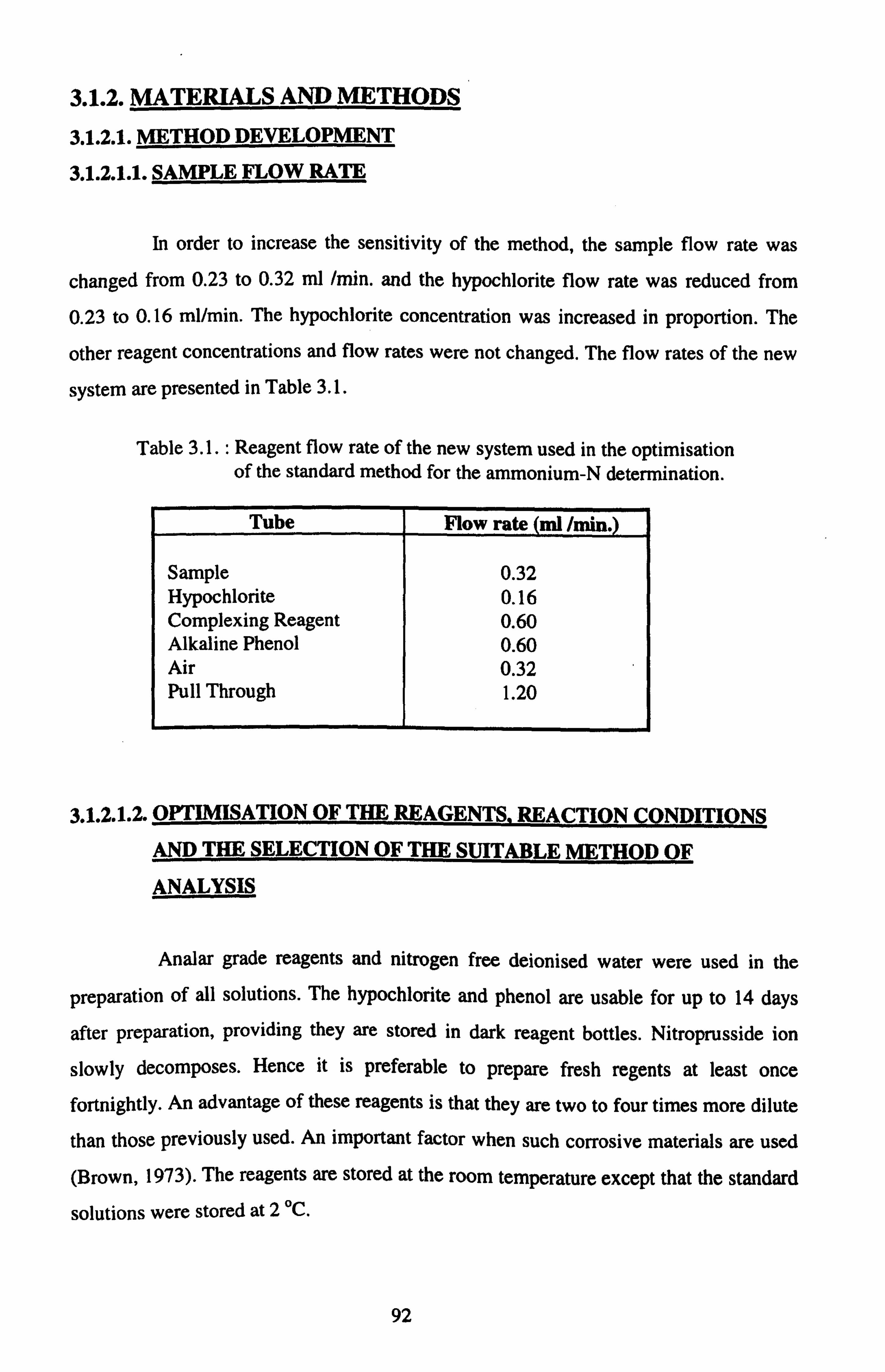
3.1.2. MATERIALS AND METHODS

3.1.2.1. METHOD DEVELOPMENT

3.1.2.1.1. SAMPLE FLOW RATE

In order to increase the sensitivity of the method, the sample flow rate was

changed from 0.23 to 0.32 ml /min. and the hypochlorite flow rate was reduced from

0.23 to 0.16 ml/min. The hypochlorite concentration was increased in proportion. The

other reagent concentrations and flow rates were not changed. The flow rates of the new

system are presented in Table 3.1.

Table 3.1.: Reagent flow rate of the new system used in the optimisation of the standard method for the ammonium-N determination.

Tube Flow rate ml /min.

Sample 0.32 Hypochlorite 0.16 Complexing Reagent 0.60 Alkaline Phenol 0.60 Air 0.32 Pull Through 1.20

3.1.2.1.2. OPTIMISATION OF THE REAGENTS. REACTION CONDITIONS

AND THE SELECTION OF THE SUITABLE METHOD OF

ANALYSIS

Analar grade reagents and nitrogen free deionised water were used in the

preparation of all solutions. The hypochlorite and phenol are usable for up to 14 days

after preparation, providing they are stored in dark reagent bottles. Nitroprusside ion

slowly decomposes. Hence it is preferable to prepare fresh regents at least once

fortnightly. An advantage of these reagents is that they are two to four times more dilute

than those previously used. An important factor when such corrosive materials are used

(Brown, 1973). The reagents are stored at the room temperature except that the standard

solutions were stored at 2 T.

92

This optimisation was carried out by two different methods of analysis :

(a)- INDIVIDUAL CONCENTRATION METHOD :

In this method the reagents and the reaction conditions were kept constant ,

one reagent was chosen to be tested and different concentrations were prepared . These

different concentrations were run individually with 1.0 mg /1 NH4-N standard solution to

get the optimum concentration of this reagent.

PROCEDURE:

The start - up procedure was followed and the system was allowed to

equilibrate with a particular test solution concentration. When the chart tracing reached

a stable base line, 1.0 mg /1 NH4-N standard solution was run with STD CAL set at 1.

This was repeated for each test concentration.

(b)- GRADIENT CONCENTRATION METHOD :

In this method there is a 250 ml reservoir beaker containing a constant

volume of deionised water (100 ml). There is Flow In containing the concentrated test

reagent and there is Flow Out going to the system containing the reagent whose

concentration increases gradually with time. The flow rate was the same to maintain an

equal volume in the reservoir beaker. This is shown in Figure 3.2.

The concentration of the reagent at any time can be calculated from the

following equation :

R=C [1 -ev l

Where :

R= Reagent concentration

F= Flow rate

v= loo ml

93

t= Time (the time required for drawing 0.5 inch of the peak = 6.0 minutes and 30

seconds). C= Concentration of the concentrated test reagent.

PROCEDURE:


equilibrate. When the chart tracing reached a stable base -line, 1.0 mg /1 NH4-N standard

solution was run with STD CAL set at 1 with the increasing concentration of the test

reagent.

Pump

Extra tube

Concentrated --b- Test Reagent

__ý__

To the chemical manifold reaction

Concentrated Test Reagent Tube

Flow In -III 11 4- Flow Out

-: ý=

s. _. Reservoir Beaker

A- Magnetic stirrer

Figure 3.2.: System for continuous gradient method.

3.1.2.1.2.1. OPTIMISATION OF THE PHENOL CONCENTRATION

The following individual concentrations of phenol were tested :

0.0,30,40,50,60 g phenol /litre of sodium hydroxide solution. The NaOH

solution was standardised at 22.5 g NaOH / litre deionised water. All the reaction

94

conditions and other non optimised reagents were kept constant throughout. This test

was carried out in one run.

3.1.2.1.2.2. OPTIMISATION OF THE SODIUM HYDROXIDE

CONCENTRATION AND THE uH

The following individual concentrations of sodium hydroxide were tested : 15,20,22.5,25,30,35 g sodium hydroxide / litre of alkaline phenol

solution. The phenol solution was standardised at 50 g /l. All other reaction conditions

and other non optimised reagents were kept constant throughout. This test was carried

out in one run.

The pH was measured for each solution of these sodium hydroxide tested

solutions by the pH meter.

PROCEDURE:

The pH meter was connected to the system as shown in Figure 3.3. The pH

meter and a combined glass / reference electrode was first standardised with buffer

solutions of pH 7 and 4. The start - up procedure was followed and the system was

allowed to equilibrate. When the chart tracing reached a stable base line, 1.0 mg /1 NH4-

N standard solution was run with STD CAL set at I. pH was monitored continuously

throughout each run for the different NaOH solutions.

95

Figure 3.3.: Flow cell for measuring pH of the flow stream at the colorimeter outlet.

3.1.2.1.2.3. OPTIMISATION OF POTASSIUM SODIUM TARTRATE AND SODIUM CITRATE CONCENTRATIONS

The following individual concentrations of potassium sodium tartrate and

sodium citrate were tested :

30 g potassium sodium tartrate + 30 g sodium citrate, 40 g potassium sodium tartrate + 40 g sodium citrate, 50 g potassium sodium tartrate + 50 g sodium citrate, 60 g

potassium sodium tartrate + 60 g sodium citrate and 70 g potassium sodium tartrate + 70

96

g sodium citrate in litre of sodium nitroprusside solution. The sodium nitroprusside

solution was standardised at 0.5 g sodium nitroprusside and the wetting agent was added

at 1 ml 15% Brij. -35 solution /litre. All the reaction conditions and other non optimised

reagents were kept constant throughout. This test was carried out in two runs.

3.1.2.1.2.4. OPTIMISATION OF THE SODIUM NITROPRUSSIDE

CONCENTRATION

INDIVIDUAL CONCENTRATION METHOD :

The following individual concentrations of sodium nitroprusside were tested.

These concentrations of sodium nitroprusside were normalised on common base and

were listed as follows :

0.2,0.25,0.3,0.4,0.5,0.6,1.0,1.5 and 2.0 g sodium nitroprusside / litre of

complexing reagent solution. The complexing reagent solution was standardised at 50 g

potassium sodium tartrate + 50 g sodium citrate and the wetting agent was added at 1

ml 15% Brij. -35 solution /litre. All the reaction conditions and other non optimised

reagents were kept constant throughout. This test was carried out in 3 runs.

A further test was carried out to study the effect of different concentrations of

sodium nitroprusside on the base line by using 0.0 mg /1 NH4-N standard solution . The

following individual concentrations of sodium nitroprusside were tested : 0.2,0.3,0.4,

0.5 and 0.6 g sodium nitroprusside / litre of the complexing reagent solution. All the

reaction conditions and other non optimised reagents were kept constant. This test was

accomplished in two runs. Each run was done as above.

GRADIENT CONCENTRATION METHOD :

An increasing concentration of sodium nitroprusside was tested. This

increasing concentration of sodium nitroprusside was obtained using the following :

Flow In, Flow out (0.6 ml/min. ).

Reservoir Beaker contained 100 ml of complexing reagent solution (free of sodium

nitroprusside) which was standardised at 5g potassium sodium tartrate +5g sodium

citrate and the wetting agent was added at 0.1 ml 15% Brij. -35 solution / 100 ml

deionised water.

97

Concentrated test reagent was 100 ml of complexing reagent solution (concentrated

sodium nitroprusside) which was standardised at 5g potassium sodium tartrate +5g

sodium citrate +1g sodium nitroprusside and the wetting agent was added at 0.1 ml

15% Brij. -35 solution / 100 ml deionised water.

All the reaction conditions and other non optimised reagents were kept

constant throughout. This test was carried out in 2 runs.

A further test was carried out to study the effect of the increasing

concentration of sodium nitroprusside on the base line by using 0.0 mg /1 NH4-N

standard solution. This test was carried out in 2 runs.

3.1.2.1.2.5. OPTIMISATION OF THE SODIUM HYPOCHLORITE

CONCENTRATION

INDIVIDUAL CONCENTRATION METHOD :

The following individual concentrations of sodium hypochlorite were tested : 5,10,20,30,40,50,60 and 70 ml sodium hypochlorite solution / litre. All

the reaction conditions and other non optimised reagents were kept constant throughout.

This test was carried out in 3 runs.

GRADIENT CONCENTRATION METHOD :

An increasing concentration of sodium hypochlorite was tested. This

increasing concentration of sodium hypochlorite was obtained using the following :

Flow In, Flow Out (0.16 ml /min. ).

Reservoir Beaker contained 100 ml deionised water.

Concentrated test reagent was 50 ml of concentrated sodium hypochlorite solution. All the reaction conditions and other non optimised reagents were kept

constant throughout. This test was carried out in 2 runs. A further test was done to study the effect of the increasing concentration of

sodium hypochlorite on the base line by using 0.0 mg /I NH4-N standard solution. This

test was done in one run.

98

3.1.2.1.2.6. ABSORPTION SPECTRUM OF THE COLOURED PRODUCT

PROCEDURE:

While measuring 1.0 mg /1 NH4-N standard solution, a 10 ml sample of the

indophenol product was collected from the colorimeter outlet. The absorbance spectrum

was measured using the spectrophotometer (SHIMADZU - Model : UV 3101 PC). All

other reaction conditions and the optimised reagents were kept constant throughout.

3.1.2.1.2.7. OPTIMISATION OF THE TEMPERATURE OF THE MANIFOLD

WATER BATH

The following temperatures of the manifold water bath were tested : 10,15,21,25.5,30,35.5,40.5 and 45 C.

All other reaction conditions and the non optimised reagents were kept

constant throughout. This test was carried out in one run.

PROCEDURE:


equilibrate with a particular temperature of the manifold water bath. When the chart

tracing reached a stable base line, 1.0 mg /1 NH4-N standard solution was run with STD

CAL set at 1. This was repeated for each manifold water bath temperature.

3.1.2.1.3. ASSESSMENT OF THE PRECISION OF THE OPTIMISED METHOD FOR THE AMMONIUM DETERMINATION

20 samples of 1.0 and 5.0 mg /1 NH. -N standard solutions were analysed

separately using the Autoanalyzer sampler at 40 samples per hour.

The statistical analysis for the results was carried out by the Minitab Program

(Release 9.2).

99

3.1.3. RESULTS AND DISCUSSION

3.1.3.1. OPTIMISATION OF REAGENTS. REACTION CONDITIONS AND

THE SELECTION OF THE SUITABLE METHOD OF ANALYSIS

3.1.3.1.1. OPTIMISATION OF THE PHENOL CONCENTRATION

The effect of different concentrations of phenol on the sensitivity of the

standard ammonium method is presented in Figure 3.4. As can be seen from the figure,

the phenol concentration has an effect on the sensitivity. After an initial increase, the

sensitivity of the method is decreased by the high concentration of phenol (60 g /1 which

is equal to 21.43 g /1 in the final solution of the system).

30

25z

20-- 41- t3) .E EI

15

X 10

5

0 0 10 20 30 40 50 60 70

Phenol concentrations (gll)

Figure 3.4. : Effect of different concentrations of phenol on the sensitivity of the standard ammonium-N method.

It is recommended that the optimum concentration of phenol is 45 g /l, which

is equal to 16.07 g /1 in the final solution of the system. A similar result was obtained by

Harwood and Huyser (1970) who recommended the optimum concentration of phenol to

be 17 g /1 in the final solution.

Other authors suggested different concentrations of phenol as shown in Table

3.2.

100

Table 3.2. : Phenol concentrations of different authors for the sodium nitroprusside catalysed phenol-hypochlorite method.

Author Phenol concentration* /1)

Brown (1973) 4.95 Berg and Abdullah (1977) 4.62 Mantoura and Woodward (1983) 3.97 Tel and Jansen (1992) 12.02 Technicon Autoanalyzer 16.23 (Industrial method #624-81 W GT)

* Phenol concentration is in g phenol /1 in the final solution.

3.1.3.1.2. OPTIMISATION OF SODIUM HYDROXIDE CONCENTRATION

Figure 3.5. shows the effect of different concentrations of sodium hydroxide

on the sensitivity of the standard ammonium method. It was observed from the figure

that the optimum concentration of NaOH is 22.5 g /1 which is equal to 8.03 g /1 in the

final solution of the system but the selected concentration of NaOH is 25.0 g /1 which is

equal to 8.93 g /1 in the final solution because the curve was less steep at this point and

the slope decreased abruptly below 22.5 g A.

40-

35--

30--

25--

20-- ö eCe ýý 15

10--

5

tä0L

0 10 20 30 40 Sodium hydroxide concentrations (911)

Figure 3.5.: Effect of different concentrations of sodium hydroxide on the sensitivity of the standard ammonium-N method.

101

Other authors suggested different concentrations of sodium hydroxide as

shown in Table 3.3. The selected concentration is higher than in any of these other

methods.

Table 3.3. : Sodium hydroxide concentrations of different authors for the sodium nitroprusside catalysed phenol-hypochlorite method.

Author Sodium hydroxide concentration* (g /1


* Sodium hydroxide concentration is in g sodium hydroxide /1 in the final solution.

3.1.3.1.3. OPTIMISATION OF THE nH

Searle (1984) pointed out that as the reagents , catalysts and concentrations

used in the Berthelot reaction affects on the optimum pH reaction, many optimum pH

values have been suggested.

The influence of the pH on the sensitivity of the standard ammonium method is presented in Figure 3.6. It can be seen from the figure that the optimum pH is 11.7 but

the pH value 12.1 is corresponded to the selected concentration of NaOH (25 g /l, which is equal to 8.93 g /1 in the final solution). Similar result was obtained by Harwood and Huyser (1970) who indicated that pH value 12.3 gave the maximum of the indophenol-

blue colour development but pH value between 11.4 and 12.3 resulted in an essentially

stable colour. But lower pH optima were suggested by Mantoura and Woodward (1983);

pH of approximately 10.6 and Krom (1980); pH 10.7 - 11.1.

102

40-

35--

30--

25--

20--

15 "- c

10

5

0 9 10 11 12 13 14

pH

Figure 3.6. : Effect of the pH on the sensitivity of the standard ammonium-N method.

A higher pH values optima are often suggested when salicylic acid is used

[Krom (1980); pH 12 -13 and Doyle and Schimel (1996); pH 13.4].

3.1.3.1.4. OPTIMISATION OF THE POTASSIUM SODIUM TARTRATE AND

SODIUM CITRATE CONCENTRATIONS

The effect of different concentrations of potassium sodium tartrate and

sodium citrate on the sensitivity of the standard ammonium method is shown in Figure

3.7. It can be noticed from the figure that there is a very slight decrease in the slope of

the peak, therefore, the potassium sodium tartrate and sodium citrate concentrations

have no effect on the sensitivity.

103

40-

35--

30--

CD 25E

C 20

15

10

5

0 0 20 40 60 80

Potassium sodium tartrate and sodium citrate concentrations (9/1)

Figure 3.7. : Effect of different concentrations of potassium sodium tartrate and sodium citrate on the sensitivity of the standard ammonium-N method.

A concentration of potassium sodium tartrate and sodium citrate is 50 g /1,

which is equal to 17.86 g /1 for each in the final solution of the system, was selected.

Other authors suggested different concentrations of potassium sodium tartrate

and sodium citrate as shown in Table 3.4.

Table 3.4. : Potassium sodium tartrate and sodium citrate concentrations of different authors for the sodium nitroprusside catalysed phenol-hypochlorite method.

Author Potassium sodium Sodium citrate tartrate concentration*

concentration* (g /1) (g /1)

Berg and Abdullah (1977) -------- 23.49 Mantoura and Woodward (1983) -------- 16.67 Tel and Jansen (1992) -------- -------- Technicon Autoanalyzer 11.09 8.07 (Industrial method #624-81 W GT)

* Potassium sodium tartrate and sodium citrate concentrations are in g /1 in the final

solution.

104

Gentry and Willis (1988) used two different concentrations of 6.6 g /1 and 16.5

g /1 in the final solution for both the potassium sodium tartrate and sodium citrate in the

salicylate method. They found that the efficiency of the elimination of interferences was

much better with sodium citrate than with potassium sodium tartrate. With potassium

sodium tartrate, precipitation occurred at the point in the manifold where the sample was

mixed with ammonium reagent but dissolved shortly thereafter. With sodium citrate in

place of potassium sodium tartrate, no precipitate was formed, thus, further reinforcing

the hypothesis that citrate is the preferred reagent for eliminating interference. No

interference occurred from Ca when present at 1000 mg /1, Mg at 1000 mg /1, Fe +3 at

200 mg /1, or Fe +2 at 100 mg /1 with the use of 6.6 g /1 sodium citrate. Despite of the

slightly better results obtained when 16.5 g /1 sodium citrate was used, it was felt that

the additional quantities of sodium citrate were not justified since they resulted in

insufficient improvement.

3.1.3.1-5. OPTIMISATION OF SODIUM NITROPRUSSIDE CONCENTRATION


Figure 3.8. shows the effect of different concentrations of sodium

nitroprusside on the sensitivity of the standard ammonium method. It is obvious from

the figure that the sodium nitroprusside concentration has no effect on the sensitivity at

the levels tested. The very slight decrease in the slope may be due to the fact that there is

interaction between the required time for developing the colour and the concentration of

sodium nitroprusside. It is supposed that the optimum concentration of sodium

nitroprusside used will increase as the time period for developing the colour decreases.

105

40

35

CO 4 30

.- 25

o+ $ 20 ýEc Lö1 15--

xi 10 mw a5

0 0 0.5 1 1.5 2 2.5

Sodium nitropruseide concentrations (g /1)

"1 mg /i 0.0 mg /i

Figure 3.8. : Effect of different concentrations of sodium nitroprusside on the sensitivity of the standard ammonium-N method.

As there is a very slight change in the slope, the optimum concentration of

sodium nitroprusside can be anywhere in the slope but the chosen concentration is 0.5 g

/1, which is equal to 0.18 g /1 in the final solution of the system, because the base line

slope has the same behaviour as that of 1.0 mg /1 NH4-N standard solution. In addition,

to choose high concentration of sodium nitroprusside as optimum concentration will

cost much.


Figure 3.9. shows a graph drawn between the peak height of a 1.0 mg /1 NH4-

N standard solution and run time (minutes). Figure 3.10. shows a graph drawn between

1.0 mg /1 and 0.0 mg /1 NH4-N standard solutions and the concentration (g /1) of sodium

nitroprusside. The concentration of sodium nitroprusside was calculated using the

equation described in section 3.1.2.1.2. The base line increases with increasing sodium

nitroprusside concentration, therefore, the values for 1.0 mg /1 NH4-N have been

corrected by the subtraction of the baseline value.

106

40- z 35

z 30 E

25

e 20

15 oº r 10

5

0 05 10 15 20 25 30 35

Run time (minutes).

Figure 3.9. : Effect of sodium nitroprusside concentration on the sensitivity of the standard ammonium-N method using the gradient method.

40- 35--

Z C= 30--

Z 25

r 20

15

IV 1 0 a. 5

..... ............................................... 0

0 0.5 1 1.5 2

Sodium nitropruiide concentration (g11)

1mg/I......... 0.0mg/I

Figure 3.10.: Effect of sodium nitroprusside concentration on the sensitivity of the standard ammonium-N method using the gradient method.

From the results presented in Figure 3.10., the concentration of sodium

nitroprusside which gave the best peak height (response) is ranging from 0.15 g /1 which

is equal to 0.05 g /1 in the final solution to 1.6 g /1 which is equal to 0.57 g /1 in the final

solution. The selected concentration of sodium nitroprusside which was chosen is 0.5 g

/1 which is equal to 0.18 g /1 in the final solution.

107

A similar result was obtained by Harwood and Huyser (1970) who

recommended the optimum concentration of sodium nitroprusside to be 0.2 g /1 in the

final solution.

Other authors suggested different concentrations of sodium nitroprusside as

shown in Table 3.5.

Table 3.5.: Sodium nitroprusside concentrations of different authors for the sodium nitroprusside catalysed phenol-hypochlorite method.

Author Sodium nitroprusside concentration* /1


* Sodium nitroprusside concentration is in g sodium nitroprusside /1 in the final solution.

Comparison of the gradient concentration method with the individual

concentration method shows that the gradient method does not give the precise estimate

and this may be due to that the gradient peak is not linear in terms of the concentration

as well as there is shifting in the base line.

3.1.3.1.6. OPTIMISATION OF SODIUM HYPOCHLORITE CONCENTRATION


The effect of different concentrations of sodium hypochlorite on the

sensitivity of the standard ammonium method is illustrated in Figure 3.11.

108

40-

zs

z 25

T 20

OC GV

15

10

5

0 0 20 40 60 80

Sodium hypochlorite concentrations (mill)

Figure 3.11.: Effect of different concentrations of sodium hypochlorite on the sensitivity of the standard ammonium-N method.

From the results obtained, it is recommended that the optimum concentration

of sodium hypochlorite is 50 ml /1, which is equal to 4.76 ml /1 in the final solution of

the system.


Figure 3.12. shows a graph drawn between the peak height of a 1.0 mg /1

NHa-N standard solution and run time (minutes). Figure 3.13. shows a graph drawn

between 1.0 mg /1 and 0.0 mg /1 NH4-N standard solutions and the concentration (g /1) of

sodium hypochlorite. The concentration of sodium hypochlorite was calculated using the

equation described in section 3.1.2.1.2. The base line increases with increasing sodium

hypochlorite concentration, therefore, the values for 1.0 mg /1 NH4-N have been

corrected by the subtraction of the baseline value.

109

40-

z 35--

z C E -E 25

20--

15--

lo--

5-

0-

0 10 20 30 40 50 60

Run time (minutes).

Figure 3.12. : Effect of sodium hypochlorite concentration on the sensitivity of the standard ammonium-N method using the gradient method.

30- i

.8 25

CC

E 20 r Ö

ý= 15 °'c

.wE 10

0 da 5-

................................... 0

0 20 40 60 80 100 Sodium hypochlorits concentration (ml/1)

1-1 mgn --------- 0. Omg/I

Figure 3.13. : Effect of sodium hypochlorite concentration on the sensitivity of the standard ammonium-N method using the gradient method.

From the results obtained in Figures 3.12. and 3.13., the selected

concentration of sodium hypochlorite which gave the best peak height (response) for 1.0

110

mg /1 NH4-N standard solution is 50 ml sodium hypochlorite /1 which is equal to 4.76

ml /1 in the final solution.

Similar results were obtained by Khan (1994) who studied the effect of

different concentrations of hypochlorite on the interference caused by the amino acids in

the phenol method. He found that all the amino acids tested caused negative interference

but the negative interferences were much reduced with the use of 50 ml hypochlorite A.

Searle (1984) also reported that negative interferences through the reactions

between amino acids and the hypochlorite source occurs with very low hypochlorite

concentrations.

Harwood and Huyser (1970) recommended the optimum concentration of

sodium hypochlorite to be 0.5 ml /l in the final solution.

Other authors suggested different concentrations of sodium hypochlorite as

shown in Table 3.6.

Table 3.6. : Sodium hypochiorite concentrations of different authors for the sodium nitroprusside catalysed phenol-hypochlorite method.

Author Sodium hypochlorite concentration* ml /1)

Brown (1973) 3.83 Tel and Jansen (1992) 16.21 Technicon Autoanalyzer 11.20 (Industrial method #624-81 W GT)

* Sodium hypochlonte concentration is in ml sodium hypochlorite /1 in the final solution.

3.1.3.1.7. ABSORPTION SPECTRUM OF THE COLOURED PRODUCT

Figure 3.14. shows the absorbance of the coloured product. It was observed

from the figure that the maximum absorbance of the coloured product is at wavelength

equal to 640 - 650 nm. Therefore, it is recommended that 650 nm filter can be used

effectively providing high sensitivity.

Other authors suggested different wavelengths of filter as shown in Table 3.7.

111

Table 3.7. : Wavelength of filter of different authors for the sodium nitroprusside catalysed phenol-hypochiorite method.

Author Wavelength of filter (nm)

Harwood and Huyser (1970) 625 Brown (1973) 625 Berg and Abdullah (1977) 625 Mantoura and Woodward (1983) 630 Tel and Jansen (1992) 660 Technicon Autoanalyzer 630 (Industrial method #624-81 W GT)

Krom (1980) used a salicylate method and demonstrated that the X m. , was

650 - 660 nm for all combinations of reactants and reaction conditions. There were however, slight differences in the spectrum produced using aquopentacyanoferrate (In

[AqF] and sodium nitroprusside catalysts and with sodium nitroprusside between

development of the colour at 35 °C in room lightening compared with at 20 °C in the

dark.

112

Absorbance

0

U' 0 0 C

ic

r 0 q

70

I

J O O

0

Figure 3.14. : Absorption spectrum of the indophenol product.

113

3.1.3.1.8. OPTIMISATION OF THE TEMPERATURE OF THE MANIFOLD

WATER BATH

The effect of different temperatures of the manifold water bath on the

sensitivity of the standard ammonium method is presented in Figure 3.15. The optimum

temperature is 30 °C, but from the results obtained there is little difference in the peak

height over the range 30 - 45 °C. As the water bath is normally operated at 37 °C for the

other determinations, it was decided to continue to use 37 °C for the ammonium-N

method.

35

30

Z 25 c E 20

ý 15

10

5

0 0 10 20 30 40 50

Manifold water bath temperature (C)

Figure 3.15. : Effect of different temperatures of the manifold water bath on the sensitivity of the standard ammonium-N method.

Other authors suggested different temperatures for the manifold water bath as

shown in Table 3.8.

114

Table 3.8. : Manifold water bath temperature of different authors for the sodium nitroprusside catalysed phenol-hypochlorite method.

Author Manifold water bath temperature C


Doyle and Schimel (1996) used the salicylate method and concluded that

raising the temperature from 30 to 60 °C doubled the indophenol absorbance. Although

the indophenol colour is less stable at high temperatures ( Searle, 1984), high

temperature accelerates colour development which Doyle and Schimel considered to be

useful for the rapid automated analysis.

Having made these optimisations to the standard ammonium-N method, the

final method is shown in section 3.1.3.2.

115

3.1.3.2. FINAL METHOD FOR THE DETERMINATION OF AMMONIUM

REAGENTS :

Analar grade reagents and nitrogen free deionised water were used





cleared immediately. When finished, the balance was wiped down and returned to the



****** Phenol is highly toxic and caustic. Preparation of this reagent should

be carried out in the fume cupboard. Ensure that you are familiar with the MSDS sheet


25 g of sodium hydroxide was dissolved in approximately 900 ml deionised

water in a1 litre dark glass bottle and then the solution was cooled to room temperature.

Working in a fume cupboard, 45 g phenol was weighed very carefully into a1 litre

beaker. Approximately 500 ml sodium hydroxide solution was added and the contents

were stirred carefully with a glass rod to dissolve the phenol. Further sodium hydroxide

solution was added if necessary. The solution was returned to the bottle and degassed in

the ultrasonic bath for 10 minutes. The volume was made to 1 litre with degassed

deionised water and the contents were mixed gently. A plastic stopper was used not a

glass one.



in a fume cupboard. ******

50 g potassium sodium tartrate and 50 g sodium citrate were dissolved in

approximately 900 ml deionised water in a1 litre bottle and degassed. 0.5 g sodium

116

nitroprusside was weighed carefully into a 100 ml beaker, 50 ml degassed deionised

water was added and the contents were stirred gently using a magnetic stirrer. The

resulting solution was added to the citrate tartrate solution and degassed in the ultrasonic

bath for 10 minutes. 1.0 ml of 15% Brij-35 solution was added and the volume was

made to 1 litre with degassed deionised water and the contents were mixed gently.

(c)- Sodium Hypochlorite Solution (Approximately 0.5 %) :


chlorine gas with acids. This reagent should be prepared in a fume cupboard. *****


available chlorine) was added to I litre degassed deionised water and the contents were

mixed gently.

(d)- Ammonium nitrogen standard stock solution (1000 mg /1) :

Ammonium sulphate was dried at 105 °C for 1 hour and cooled in a

desiccator for 30 minutes. 4.717 g of dry ammonium sulphate was dissolved in


made to 1 litre with deionised water. The solution was stored at 2 T. Working standards


PROCEDURE:

The manifold (Figure 3.16. ) can be used for the determination of ammonium in water, 2.0 M and 1.0 M potassium chloride, 0.5 M potassium sulphate and several

other extractants. The flow rate of the final system is shown in Table 3.9.

117

To waste

5 turns 10 turns 10 turns

To waste coil coil coil


Delay coil 3 minutes, 37 °C 1.0 Sample wash


Figure 3.16. : Technicon Autoanalyzer II manifold of the final method for the determination of NH. -N.

Table 3.9. : Reagent flow rate of the optimised method for the NH4-N determination.

Tube Flow rate ml /min.

Sample 0.32 Hypochlorite 0.16 Complexing Reagent 0.60 Alkaline Phenol 0.60 Air 0.32 Pull Through 1.20

The solutions can be analysed using the manifold shown in Figure 3.16. along

with standard solutions, blanks and zeros. The samples can be run at the rate of 50 per

10 turns Sample

coil Water

0.8 Air

0.32 Resample


0.60 Phenol

0.32 Air

0.16 Hypochlorite

118

hour but where dilution is required the sampling rate is reduced to 40 per hour. The

colour is developed in the manifold water bath at 37 °C. The colour intensity is

measured at 650 nm. The air is cleaned of atmospheric ammonia by bubbling through

5.0 % HCl solution. The calibration graph for ammonium is linear from 0.0 to 5.0 mg

NH4-N A. Samples with ammonium - nitrogen concentrations higher than 5.0 mg /1 are

diluted into the range 0.0 to 5.0 mg /1 using an inbuilt diluter. Appropriate dilution is

carried out for concentrations above 5.0 mg /1. The selected pH for this system is 12.1.

119

3.1.3.3. ASSESSMENT OF THE PRECISION OF THE OPTIMISED METHOD

FOR THE AMMONIUM DETERMINATION

The precision of the optimised method was evaluated by analysing 20

samples of 1.0 and 5.0 mg /1 NH4-N standard solutions using the Autoanalyzer sampler

at 40 samples per hour.

The standard deviation (STDEV) and relative standard deviation (RSD %)

values are presented in Table 3.10. The results are very reproducible as shown by the

low RSD % and are considered acceptable since they are less than 0.5 %.

Table 3.10.: The precision of the optimised method for the ammonium determination.

Standard concentration

Sampling rate STDEV RSD %

1.0 mg /1 NH4-N 40 samples per hour 1.190 0.12

5.0 mg /1 NH4-N 40 samples per hour 4.170 0.08

Mazumder (1992) obtained an RSD % as good as 0.18 to 0.40 % for the

unoptimised standard method (section 2.11.1.1. ) using 10 replicates of 1.0 mg /1 NH4-N

standard solution.

Khan (1994) investigated the precision of the unoptimised standard method

with the inclusion of a gas phase dialyser and obtained an RSD % of 0.66 % for 1.0 mg

/1 NH4-N standard solution.

Comparison of the optimised method with those of other authors shows that

it has very good RSD % values and is suitable for the analysis of ammonium-N in soil

and water.

120

3.2. DETERMINATION OF LOW LEVELS OF AMMONIUM

(< 0.1 mg N/ 1) IN GROUNDWATER

3.2.1. INTRODUCTION

In uncontaminated rivers, streams, groundwater and lakes, the ammonium

concentration is very low. In general, ammonia and ammonium compounds occur in

relatively small quantities in unpolluted waters, on the order of 0.1 mg /1, but organic

pollution can result in higher levels. The determination of low levels of ammonium is

important for drinking waters, certain surface waters and arctic and glacial ice. At the

pH range from 7.4 to 8.5, ammonia is considered to be toxic to diatoms at a level of 1.1

mg /1, and at the same pH range, to fish at a level of 2.5 mg /I (Zadorojny et al., 1973).

Accurate measurements below micromolar concentrations are required since ammonium

ions are a micronutrient in seawaters. Inadequate sensitivity occurs when methods such

as those based on the Nesseler and Berthelot (indophenol blue) reactions are used

(Schulze et al., 1988).

Zadorojny et al. (1973) evaluated a manual phenol - hypochlorite method

capable of determining low levels of ammonium-N. They considered it a method well

suitable for routine ammonia analyses in fresh, estuarine and marine waters and in

wastewaters since no major interferences are caused by electrolytes, amino acids, urea,

or variations in salinity. The following shows the range of ammonia determination : With intensifier :

Using a 10 - cm cuvette : 0.001 to 0.10 mg /I NH4-N.

Using a1- cm cuvette : 0.01 to 1.0 mg /1 NH4-N.

Without intensifier : Using a1- cm cuvette : 1.0 to 50 mg /1 NH4-N.

Krom (1980) noted that when sodium nitroprusside is used for the

determination of low levels of ammonia, as in sea or lake waters, variable blank values

occur through the light - induced production of an absorbing species with a spectrum

similar to the blue indophenol dye produced from ammonia.

Hara et al. (1988) developed a simple concentrator based on a microporous

poly (tetrafluoroethylene) membrane and polymer nets and combined with an ammonia -

121

selective gas electrode to construct a continuous flow determination system for low

concentrations of ammonium ions in water. A ten - fold increase in the concentration of

ammonium ions as well as extension in the linear response limit of an ammonia -

selective gas electrode from 30 to about 3µg /1 were obtained when the gas dialysis

concentrator was used. The system was used in the determination of residual

concentrations of ammonium ions in water purified by distillation and/or de - ionisation

and in natural water analysis.

Schulze et al. (1988) investigated several flow - injection methods for their

suitability for determining submicromolar levels of ammonium ion on a routine basis.

They found that the Nesseler and the Berthelot reactions are not sufficiently sensitive

but the gas - diffusion separation is more satisfactory. As the optimised gas - diffusion

conditions was used, spectrophotometric detection with an acid - base indicator or the

application of a liquid - membrane ammonium - sensitive electrode gives detection

limits around 0.14 µg /1. Problems with baseline stability and long - term drift occurs

due to the interference of carbon dioxide in the acid - base indicator method.

Contamination due to ammonium present in water and reagents severely limited the

enhancement of sensitivity by preconcentration. However, effective preconcentration

(20 fold in I min. ) is obtained when the ion - exchange microcolumn placed in the

injection loop of the valve was used. With regard to the optimisation of the flow - injection manifold, the choice of acceptor flow rate was critical. For example, at low

flow rates, by decreasing the response time of the electrode, the high sensitivity can be

counterbalanced. Despite the high sensitivity obtained by the lowest flow rate, these

conditions were unsuitable for most analytical applications due to unstable baseline,

poor reproducibility (ca. 10 %) and low sample frequency (15 /h). The use of

potentiometric detection with a liquid - membrane ammonium - sensitive electrode gave

improved baseline stability and slightly better sensitivity. However, regarding the

improved detection limits, the limiting factor is the contamination problem. Under

normal laboratory conditions, it is difficult to keep the background level present in

aqueous solutions below 0.14 µg /1. Therefore, for submicromolar ammonium

determinations, the final choice of method must be guided by particular analytical

requirements. Doval et al. (1997) introduced an update of the Kjeldahl method for the

direct determination of dissolved organic nitrogen (DON) in seawater. They reported

122

that the previous removal of dissolved inorganic nitrogen is carried out as follows :

ammonium as NH3 with NaOH at pH 9.4, and subsequently, nitrate and nitrite as nitric

oxide with FeSO4 in acid medium. The sample is then mineralized to ammonium, which

is measured with a Technicon Autoanalyzer by the indophenol blue method with a range

of 14 - 700 µg /1 NH4-N at 630 nm. Comparison showed that the tested standard

compounds gave a range of recovery similar to those obtained by high temperature

oxidation techniques. Improvement in precision was obtained by the direct

determination of DON using the method described, as shown from the comparison with

other methods the seawater samples had standard deviation of ± 2.8 p. g /1. The precision

of ammonium is ± 0.7 gg /1. Dissolved inorganic nitrogen analysis is not a critical factor

for the precision of DON measurements. DON values ranged between 42 and 140 µg /1

in several stations in the Northeast Atlantic Ocean.

The objective of this study was to develop a reliable Technicon Autoanalyzer

method to determine low levels of ammonium in groundwater (< 0.1 mg /1).

The proposed method is based on the optimised reagent concentrations

developed earlier. Using more concentrated reagents with lower flow rates enables a

larger sample flow rate to be used whilst maintaining the same reagent concentrations in

the final reagent stream. This potentially offered a3 fold increase in sensitivity

compared with the standard method (Section 2.11.1.1. ).

123


3.2.2.1. METHOD DEVELOPMENT


developed earlier. Using more concentrated reagents with lower flow rates enables a larger sample flow rate to be used whilst maintaining the same reagent concentrations in


compared with the standard method (section 2.11.1.1. ).

The samples can be run at the rate of 40 samples per hour. The colour is

developed in the manifold water bath at 37 °C. The colour intensity is measured at 650

nm. The air is cleaned of atmospheric ammonia by bubbling through 5% HCl solution.

As part of the method developing, the following parameters were tested : 1- Effect of the potassium sodium tartrate and sodium citrate concentrations on the

solubility of the high concentration complexing reagent solution.

2- Assessment of the pulse suppresser tubes.

3- Assessment of the sequence of adding reagents.

4- Assessment of the sample line debubbler.

5- Assessment of the precision of the final method.

The development work was primarily concerned with obtaining satisfactory

low noise levels and good peak shape. The tests of each modification of the system were

carried out as follows :


equilibrate. When the chart tracing reached a stable base line, 1.0 mg /1 NH4-N standard

solution was run continuously with STD CAL set at 1.0 to observe the noise level on the

peak. When the chart tracing reached a stable base line again, 6 samples of 1.0 mg It

NH4-N standard solution were analysed using the Autoanalyzer sampler at 40 samples

per hour to observe the peak shape and to ensure that a peak with a flat top was

obtained.

124

3.2.2.1.1. EFFECT OF THE POTASSIUM SODIUM TARTRATE AND SODIUM

CITRATE CONCENTRATIONS ON THE SOLUBILITY OF THE

HIGH CONCENTRATION COMPLEXING REAGENT SOLUTION

Different solutions of potassium sodium tartrate and sodium citrate were prepared

to determine the combined solubility. These solutions were prepared as follows :

Solution Potassium Sodium Tartrate Sodium Citrate No. (g /1) (g /1)

1 50.0 50.0 2 50.0 75.0 3 50.0 100.0 4 50.0 125.0 5 75.0 50.0 6 75.0 75.0 7 75.0 100.0 8 75.0 125.0 9 100.0 50.0

10 100.0 75.0 11 100.0 100.0 12 100.0 125.0 13 125.0 50.0 14 125.0 75.0 15 125.0 100.0 16 125.0 125.0

All solutions contained 1.0 g sodium nitroprusside and 1.0 ml 15% Brij. -35 solution.

3.2.2.1.2. ASSESSMENT OF THE PULSE SUPPRESSER TUBES

The following pulse suppresser tubes were tested :

1- Long tubing [Internal diameter = 0.38 mm and length = 43 cm].

2- Short tubing [Internal diameter = 0.38 mm and length = 21.5 cm].

125

3.2.2.1.3. CHOICE OF THE SEQUENCE OF ADDING REAGENTS

The following sequences of adding reagent were tested : 1- Sequence No. 1:

a- Debubbled sample.

b- Air bubble.

c- Phenol and complexing reagent solutions pre mixed with stream divider. d- Hypochlorite.

2- Sequence No. 2:


b- Air bubble.

c- Phenol, complexing reagent and hypochlorite pre mixed with stream divider.

3- Sequence No. 3:

a- Phenol, complexing reagent and hypochlorite solutions pre mixed with stream divider.

b- Air bubble.

c- Debubbled sample.

4- Sequence No. 4:


b- Air bubble.

c- Phenol solution. d- Complexing reagent solution.

e- Hypochlorite solution.

126

Air Debubbler

4 A10

1 AlO Sample

j4

Hypochlorite -*

Phenol -p. +--- Complexing Reagent

t Stream Divider PT1I

Where : A 10 T Junction= 116 B034 01 Stream Divider PT11 = 116 B043 01

Sequence No. I

Air Debubbler 44

AlO Sample

4

Stream s- Hypochlorite Divider BT 10 Complexing Reagent

. -- Phenol

Where : A 10 T Junction = 116 B034 01 Stream Divider BT10 = 116 B042 01

Sequence No. 2

127

Stream Air Divider BT 10

AlO Phenol

Debubbled Sample Hypochlorite -º

1 Complexing Reagent

Where : A 10 T Junction = 116B03401 Stream Divider BT10 = 116 B042 01

Sequence No. 3

Air Debubbler 44

Sample A10 A10 A10 4

444

4--- Phenol

f-- Complexing Reagent

4Hypochlorite

Where : A 10 T Junction =; 116 B034 01

Sequence No. 4

128

3.2.2.1.4. ASSESSMENT OF THE SAMPLE LINE DEBUBBLERS

The following different sizes and shapes of the sample line debubbler were tested :

1-T shape debubbler unit No. 1:

Liquid Stream (ID = 1.8 mm).

Debubbling Stream (ID = 1.8 mm).

Both corners well rounded.

2- T shape debubbler unit No. 2:

Liquid Stream (ID = 2.3 mm)










Both corners rather squarer.




The leading corner rounded, the tailing corner squarer.

6- Technicon fitting [T 021 600101] :



129

Internal Diameter = 1.8 mm 1

[Debubbling Stream]

-'-"r . -- Internal Diameter = 1.8 mm [Liquid Stream]

T Shape Debubbler Unit No. 1

ID =2.3mm


ID =2.3mm 4

_JL_

d- ID =2.3rnm

4-ID=1.8mm


130

ID = 2.3 mm 4

ý--ID=1.8mm

T Shape Debubbler Unit No. 4.

ID =2.3mm

IL

"- ID = 1.8 mm

Direction of flow


1.2 mm 2.0 mm [Debubbling Stream] 44

][j

- . &-- 2.0 mm 2.0 mm --ý [Liquid Stream]

Technicon Fitting If 021 0001 01 ]

131

3.2.2.2. ASSESSMENT OF THE PRECISION OF THE FINAL METHOD

20 samples of 1.0 and 0.1 mg Il NH4-N standard solutions were analysed

separately at 30 and 40 samples per hour.

The statistical analysis for the results was carried out by the Minitab Program

(Release 9.2).

132



developed earlier. Using more concentrated reagents with lower flow rates enables a

larger sample flow rate to be used whilst maintaining the same reagent concentrations in


compared with the standard method (section 2.11.1.1. ).

The flow rate and recalculated reagent concentrations of the proposed method

are summarised in Table 3.11. The proposed reagent concentrations were obtained by

rounding the recalculated reagent concentrations. The schematic diagram of the

proposed method is shown in Figure 3.17.

To waste

10 turns 10 turns 10 turns To waste coil coil coil


Delay coil 3 minutes, 37 °C

10 turns Sample

coil Water E 0.8 Air

0.32 Air

0.42 Debubbler

1.4 Resample


0.23 Phenol

0.16 Hypochlorite

1.0 Sample wash

1.2 Colorimeteric pull through

Figure 3.17. : Technicon Autoanalyzer II manifold of the proposed method for the determination of low level of NH4-N in groundwater.

133

Table 3.11. : Flow rates, recalculated and proposed reagent concentrations.

Reagent Flow rate tnl / min. )

Recalculated concentration

Proposed concentration

- Sample* 1.40

- Sample line debubbler 0.42

- Sodium Hypochlorite 0.16 47.62 ml /1 50.00 ml /1

-Complexing Reagent : 0.23

a- Potassium sodium 124.22 g /1 100.00 g /1 tartrate

b- Sodium citrate 124.22 g /1 100.00 g /1

c- Sodium nitroprusside 1.24 g /1 1.00 g /1

- Alkaline Phenol : 0.23

a- Phenol 111.80 g /l 110.00 g /1 b- Sodium Hydroxide 62.11 g /1 60.00 g /1

- Air 0.32

- Pull Through 1.20

Because of high sample flow rate from the tubing connecting the sample probe to the sample pump tubing the sample connecting tube was increased from ID = 0.76

mm to ID = 1.01 mm.

The problems related to developing the system were :

(a) - Preparation of the desired high concentration of a complexing reagent solution

proved to be impossible because of insufficient solubility of the potassium sodium

tartrate and sodium citrate.

(b) - The injection of the air bubble into the flow using the air bar caused a backwards

flow into the debubbler, therefore, a pulse suppresser tube was used in the air to

eliminate this problem.

(c) - There is a large inter sample air bubble and this should be removed. Therefore,

a sample line debubbler was used to remove the air bubbles from the sample

before the reagents were added to the sample. The flow rate of the sample is set

to 1.40 ml /min. and the sample line debubbler takes 0.42 ml /min. of the sample

to the waste. Therefore, the flow rate of the sample was designed to be 0.98

ml /min.

134

3.2.3.1. EFFECT OF THE POTASSIUM SODIUM TARTRATE AND SODIUM

CITRATE CONCENTRATIONS ON THE SOLUBILITY OF THE HIGH

CONCENTRATION COMPLEXING REAGENT SOLUTION

The complexing reagent solution was prepared based on the recalculated

concentration (Table 3.11. ) but there was a precipitation in the solution. Therefore, a

range of complexing reagent solutions of different concentrations of potassium sodium

tartrate and sodium citrate were prepared to obtain the best (clear) solution which had no

precipitation. Table 3.12. shows the solubility of each of these solutions of potassium

sodium tartrate and sodium citrate. As can be seen from the results, the precipitation

occurred in the solution as a result of increasing the concentration of potassium sodium

tartrate and sodium citrate. As the complexing reagent solution should contain as high as

concentration of potassium sodium tartrate and sodium citrate as possible, it is

recommended that the concentration of 100 g potassium sodium tartrate + 100 g sodium

citrate /I is used.

Table 3.12. : Effect of the concentrations of potassium sodium tartrate and sodium citrate on the solubility of the high concentration complexing reagent solution.

Reagent 50 g sodium 75 g sodium 100 g sodium 125 g sodium citrate /1 citrate /1 citrate /1 citrate /1

50 g potassium sodium tartrate /1 Clear Clear Clear Clear 75 g potassium sodium tartrate /1 Clear Clear Clear Clear 100 g potassium sodium tartrate /1 Clear Clear Clear Cloudy 125 g potassium sodium tartrate /1 Clear Clear loud Cloudy

From section 3.1.3.1.4., it is clear that all the concentrations of the potassium

sodium tartrate and sodium citrate have no effect on the sensitivity of the method,

therefore, the reduction in the concentration from 124.22 g /1 to 100 g /1 would not be

expected to have any impact.

135

3.2.3.2. ASSESSMENT OF THE PULSE SUPPRESSER TUBES

While running the system, the injection of the air bubble into the flow using

the air bar caused a backwards flow into the debubbler, therefore, a pulse suppresser

tube was used in the air tube to eliminate this problem.

Two lengths (21.5 and 43 cm) of internal diameter = 0.381 mm tubing were

tested.

Table 3.13. : Assessment of the pulse suppresser tubes.

Pulse suppresser tube Peak shape of the individual peaks

Noise level in the individual peaks

Short tubing Poor (pointed) Poor

Long tubing Acceptable Acceptable

From the results obtained in Table 3.13., it is recommended that the 43 cm

pulse suppresser tube is the best one to be used.

3.2.3.3. INFLUENCE OF THE SEQUENCE OF ADDING REAGENTS ON THE

PROPOSED METHOD

Different sequences of adding reagents were tested since it is an essential

criteria to obtain the best response.

The susceptibility of the reaction to interferences as a result of the hydrolysis

of organic nitrogen compounds by the alkaline hypochiorite will be affected by the

sequence of adding reagents (Wearne, 1963). The influence of different sequences of

adding reagents on the sensitivity of the proposed method is presented in Table 3.14.

The assessment was based on the peak shape and the noise level in the individual peaks.

136

Table 3.14. The influence of the sequence of adding reagents on the sensitivity of the proposed method.

Reagent sequence Peak shape of the Noise level in the individual peaks individual peaks

- Sequence No. 1: Acceptable Acceptable a- Sample b- Phenol + Complexing reagent c- H ochlorite

- Sequence No. 2: Borderline Borderline a- Sample b- All reagents pre mixed

- Sequence No. 3: Poor (pointed) Borderline a- All reagents pre mixed b- Sample

- Sequence No. 4: Borderline Borderline a- Sample b- Phenol c- Complexing reagent d- Hypochlorite

Based on the peak shape and the noise level in the individual peaks, the best

sequence of adding reagents is sequence No. 1: Pre mixed phenol and complexing

reagent solutions (0.46'ml /min. ) added to the sample line (0.98 ml /min. ) followed by

the hypochlorite solution (0.16 ml /min. ). Adding smaller flows to the larger main flow

gave a smooth overall flow and good peak shape.

3.2.3.4. ASSESSMENT OF THE SAMPLE LINE DEBUBBLER

A noise in the signal occurred at the moment the large inter sample air bubble

passed through the colorimeter, therefore, a sample line debubbler was tested to remove

the air bubbles from the sample.

Assessment of the debubblers was carried out qualitatively based on the peak

shape and the noise level in the individual peaks as well as the noise level in the

continuous peak.

137

Tests were made using different sizes and shapes of debubblers to establish a debubbler which gave a good smooth flow.

Table 3.15. illustrates the peak shape and the noise level for each one of these

debubblers. It can be seen from the results that there are obvious differences in the peak

shape as well as the noise level of the individual peaks. The best peak shape and the

minimum noise level in the peak was obtained by using debubbler No. 3 which was well

rounded in both corners of the T junction.

Although the debubbler No. 4 gave a good peak shape and low noise level in

the individual peaks, debubbler No. 3 gave a much smoother flow.

Table 3.15. : Assessment of the sample line debubblers.

Sample line debubbler

Noise level in the continuous peak

Peak shape of the individual peaks

Noise level in the individual peaks

Technicon fitting ND* Acceptable Acceptable

Debubbler No. 1 Acceptable Borderline Borderline


Debubbler No. 3 Acceptable Acceptable Acceptable

Debubbler No. 4 Acceptable Acceptable Acceptable


ND* = Not determined

Having made these modifications to the proposed method, the final method is

shown in section 3.2.3.5.

138

3.2.3.5. FINAL METHOD FOR THE DETERMINATION OF LOW LEVELS OF

AMMONIUM-N IN GROUNDWATER

REAGENTS :

Analar grade reagents and nitrogen free deionised water were used throughout.

These reagents were prepared in a fume cupboard. A fume cupboard was cleared and a2

figure top pan balance was set up. Care was taken to ensure that the balance was

properly locked before attempting to move it. The fan was switched off while actual

weighing was in progress but otherwise was kept running. Any spills were cleared up

immediately. When finished, the balance was wiped down and returned to the balance

bench. Finally, the fume cupboard was wiped down.


***** Phenol is highly toxic and caustic. Preparation of this reagent should be carried out in the fume cupboard. Ensure that you are familiar with the MSDS sheet


60.0 g of sodium hydroxide was dissolved in approximately 900 ml deionised

water in a1 litre dark glass bottle and the solution was cooled to room temperature.

Working in a fume cupboard, 110.0 g phenol was weighed very carefully into a1 litre

beaker. Approximately 500 ml sodium hydroxide solution was added and the contents

were stirred carefully with a glass rod to dissolve the phenol. Further sodium hydroxide

solution was added if necessary. The solution was returned to the bottle and degassed in

the ultrasonic bath for 10 minutes. The volume was made to I litre with degassed

deionised water and the contents were mixed gently. A plastic stopper was used not a

glass one.



in a fume cupboard. *****

139

100.0 g potassium sodium tartrate and 100.0 g sodium citrate were dissolved

in approximately 900 ml deionised water in a1 litre bottle and degassed for 10 minutes

in the ultrasonic bath. 1.0 g sodium nitroprusside was weighed carefully into a 100 ml

beaker, 50 ml degassed deionised water was added and the contents were stirred gently

using a magnetic stirrer. The resulting solution was added to the citrate tartrate solution

and degassed in the ultrasonic bath for 10 minutes. 1 ml of 15% Brij-35 solution was

added and the volume was made to 1 litre with degassed deionised water and the

contents were mixed gently.

(c)- Sodium Hypochlorite Solution (Approximately 0.5 %) :


chlorine gas with acids. This reagent should be prepared in a fume cupboard. *****


available chlorine) was added to 1 litre degassed deionised water and the contents were

mixed gently.

(d)- Ammonium nitrogen standard stock solution (1000 mg /l) :

Ammonium sulphate was dried at 105 °C for 1 hour and cooled in a desiccator for 30 minutes. 4.717 g of dry ammonium sulphate was dissolved in


made to 1 litre with deionised water. The solution was stored at 2 °C. Working standards


Care should be taking while preparing standards below 0.14 mg /1 NH4-N

since they are difficult to be prepared and to handle due to potentially serious

contamination problems (Schulze et al., 1988).

PROCEDURE:

The manifold (Figure 3.17. ) can be used for the determination of low levels of

ammonium-N in the groundwater (< 0.1 mg /1 ). The flow rate of the final method is

presented in Table 3.16.

140

Table 3.16. : Reagent flow rate of the final method for the determination of low levels of ammonium-N in groundwater.

Tube Flow rate (ml /min. )

Sample 1.40

Sample connecting tube (ID = 1.01 mm)

Sample line debubbler 0.42

Hypochlorite 0.16

Complexing Reagent 0.23

Alkaline Phenol 0.23

Air 0.32

Pulse Suppresser

(Length = 43 cm and ID = 0.38 mm)

Pull Through 1.20

The solutions can be analysed using the manifold shown in Figure 3.17. along

with standard solutions, blanks and zeros. The samples can be run at the rate of 40

samples per hour. The colour is developed in the manifold water bath at 37 °C. The

colour intensity is measured at 650 nm. The air is cleaned of atmospheric ammonia by

bubbling through 5% HCl solution. The calibration graph for ammonium is linear from

0.0 to 0.1 mg NH4-N /l.

141

3.2.3.6. ASSESSMENT OF THE PRECISION OF THE FINAL METHOD

The precision of the proposed method was evaluated by analysing 20 samples

of 1.0 and 0.1 mg /1 NHa-N standard solutions at 30 and 40 samples per hour.

The standard deviation (STDEV) and relative standard deviation (RSD %)

values are given in Table 3.17. The results are very reproducible as shown by the low

RSD % and are considered acceptable since they are less than 0.5 %.

Table 3.17. : The precision of the final method for the low levels of ammonium-N determination.

Standard concentration

Sampling rate STDEV RSD %

1.0 mg /I NH4-N 40 samples per hour 0.630 0.06

0.1 mg /I NH4-N 40 samples per hour 0.310 0.31

0.1 mg /1 NHa-N 30 samples per hour 0.354 0.36

Comparison of this low levels ammonium-N method with the optimised

method (section 3.1.3.3. ) shows that both have very good RSD % values (Tables 3.10.

and 3.17. ) and are suitable for analysis of low levels of NH4-N in groundwater.

Mazumder (1992) obtained an RSD % as good as 0.18 to 0.40 % for the

unoptimised standard method (section 2.11.1.1. ) using 10 replicates of 1.0 mg /1 NH4-N

standard solution. Khan (1994) investigated the precision of the unoptimised standard method

with the inclusion of a gas phase dialyser and obtained an RSD % of 0.66 % for 1.0 mg

/1 NH4-N standard solution.

142

3.3. ANALYSIS OF HIGHLY COLOURED GROUNDWATER

SAMPLES

3.3.1. INTRODUCTION

Some of the groundwater samples analysed in this work are highly coloured

and since the colorimetric analysis is used for the determination of ammonium-N,

nitrate-N, nitrite-N and chloride these samples need decolorisation.

There are two approaches in removing the colour, one is the removal by

decolorising agents and the other is using a dialysis system.

Different types of charcoal such as activated charcoal (Darco G60 and Norit),

bone charcoal, barbecue charcoal and activated coconut shell carbon were used for the

removal of the colour. Different types of polymers such as polyclar SB 100

[Polyvinylpyrrolidinone insoluble (PVPP)], polyclar AT [Polyvinylpyrrolidinone

insoluble (PVPP)] and polyvinylpyrrolidone soluble (PVP) were used for the removal of

the colour. The most commonly used adsorbent materials for the removal of colour are

activated charcoal (Darco G 60) and polyclar SB 100 [Polyvinylpyrrolidinone insoluble

(PVPP)].

Qadeer et al. (1994) conducted a study on the structure of a commercial

activated charcoal using different techniques such as X- ray diffraction, thermal

analysis, nitrogen adsorption and mercury porosimetry. They pointed out that the

efficiency of the activated charcoal depends on its physical adsorption capacity which

itself depends on the porosity and the surface properties of the adsorbent. The chemical

nature of the activated charcoal is associated with the intrinsic properties of the parent

materials as well as with the manufacturing and the activation methods. The activated

charcoal is characterised as amorphous in nature and has micro - crystalline structure as

shown in the X- ray diffraction study. The application of the pore size distribution curve

and D-R analysis of nitrogen adsorption isotherm refers to the microporous nature of the

activated charcoal with surface area 1000 m2 /g, porosity 75.74 % and pore volume 1.43

cm3 /g. The thermogravimeteric study of activated charcoal showed that the loss in

weight occurred in two distinct regions : one is endothermic (dehydration) and other is

143

exothermic (combustion). The moisture and ash contents were 11 % and 10 %,

respectively.

Lew (1983) developed a decolorisation method based on the combined use of

strong anion - exchange resins (Diaion PA308 and Duolite A- 102D) and activated

carbon (Darco G60 and Norit) instead of lead compounds for decolorising dilute

molasses solutions. He found a close agreement between the polarimetry measurements

of filtrates obtained from decolorisation by resin - carbon and those following

clarification by lead. In addition, the efficiency of the proposed decolorising reagents

was similar to that of lead. However, the filtration of the treated samples with resin and

carbon was faster than treatment with lead. The efficiency of Darco G60 in the

decolorisation was slightly better than that of Norit carbons. Compared with lead, the

less toxic decolorising reagents are readily available commercially and relatively

inexpensive.

McGeehan et al. (1989) found that the errors in the colorimetric analysis of

boron decreased with increasing the addition of decolorising charcoal. Charcoal is

effective in reducing the yellow colour resulting from the hot water extraction of soil,

however, care should be taken to avoid negative errors due to boron sorption by

charcoal. Meyer et al. (1992) found that with the exception of vermiculite, barbecue

charcoal and rice husks showed the best adsorptive qualities (67 % and 65 %,

respectively) as they removed more than 50 % of the colour from the wastewater. The

use of barbecue charcoal is economically beneficial since it is a cheap natural product

compared to activated carbon, can be regenerated for re - use in the same way as the

latter as well as it is readily available.

Samuelson and Wennergren (1977) indicated that compared with other resins,

a weakly basic anion exchanger in HSO3" form gave a better efficiency than that of

macroporous styrene - divinylbenzene polymers, acrylic acid esters and crosslinked

polyvinylpyrrolidone soluble (PVP) for colour removal. Although the crosslinked

polyvinylpyrrolidone soluble (PVP) which acts as a proton acceptor and leads to

hydrogen bonding with phenolic and carboxylic acid groups was the most effective in

removing the colour (500 nm) during the first period of the sorption, it was less effective

by the time 10 bed volumes had passed through than the HS03' form of a weakly basic

anion exchange resin (Duolite A- 4F).

144

Simpson et at. (1982) found that the removal of the natural colour of wine

was greater using decolorising carbon than using polyvinylpyrrolidone (PVPP). The

carbon treated wines had a reduction in optical density at 400 nm of approximately 30 %

which was greater than that for the PVPP treated wines.

Mattick and Rice (1981) indicated that compared to polyclar AT (PVPP),

charcoal (Darco KB) can cause variations in the tartrate concentration of the wine due to

the previous treatment of the charcoal. Moreover, the decolorisation method by the

charcoal is more time consuming.

The inclusion of a dialyser in the manifold of automated colorimetric analysis

systems has many advantages such as the removal of interferences like suspended solids

and unwanted macromolecules (for example protein) and to make an automated dilution

step (van Staden, 1995). In continuous flow analysis, the dialysis system consists of 2

flow streams, the donor stream (sample) and the acceptor stream, which are separated by

a semipermeable membrane. There are two different systems of the dialysis, one is the

liquid or aqueous phase dialysis and the other is gas phase dialysis. The liquid or

aqueous phase is the dialysis system where the ions pass through a wettable membrane

(C - membrane) which means the movement of ions is through a liquid film in the

membrane to reach a receptor stream. Thompson and Blankley (1984) used this dialysis

system for the determination of nitrate -N and nitrite - N. In addition, many authors

used this dialysis system for the determination of chloride (Araujo et al., 1995; and van

Staden, 1995).

The gas phase dialysis is the dialysis system in which the NH4-N is converted

to NH3-N and passes as a gas through a not wettable Teflon membrane. Many authors

have used this dialysis system for the determination of ammonium -N (Schulze et al.,

1988; Martelli et al., 1995; Gerendas et al., 1995; and Moskvin et al., 1998).

The objective of this study is to develop a method for decolorisation which

can cope with highly coloured groundwater samples. This investigation includes the use

of the charcoal G60 and polyclar SB 100 as decolorising agents. In addition, this study

includes the use of liquid dialysis and gas phase dialysis which can be included in the

chloride, nitrite, nitrate and ammonium manifold systems of the Technicon

Autoanalyzer II system.

145


All the decolorisation tests were carried in glass bottles so as to see the

solution clearly and to avoid the sticking of the charcoal in scratches in the plastic

bottles which could contaminate the bottles.

3.3.2.1. USING CHARCOAL G60 AND POLYCLAR SB100 FOR THE


This study is concerned with the efficiency of charcoal G60 and polyclar SB 100 in the decolorisation of water samples, the presence of impurities in the charcoal

G60 and the polyclar SB 100, cleaning the charcoal G60 and polyclar SB 100 from

impurities and the adsorption of NH4-N and N03-N from solution by the cleaned

charcoal G60 or polyclar SB 100.

3.3.2.1.1. EFFICIENCY OF CHARCOAL G60 AND POLYCLAR SB100 IN THE


Two decolorising agents, polyclar SB 100 and charcoal G60 were used.

MATERIALS :

1- Polyclar SB100 (polyvinylpyrrolidone insoluble) :

Polyclar SB 100 was supplied by BDH Co. It is an insoluble cross - linked

polyvinylpyrrolidone, useful for purification of plant enzymes by absorbing phenols and

tannins from aqueous extracts [BDH Laboratory Supplies Catalogue, 1997]. Polyclar is

a registered Trade Mark of GAF Corporation. NR.

2- Charcoal decolorising powder activated (Darco G60) :

Charcoal G60 was supplied by BDH Co. Darco is the registered trade mark

of Norit U. K. Ltd. NR. [BDH Laboratory Supplies Catalogue, 1997].

146

This experiment was carried out on 2 groundwater samples (SW 15 and SW

16) which differed in colour and pH as shown in Table 3.18. These groundwater

samples were collected from Nobel Enterprises, Ardeer site, Stevenston Ayrshire,

Scotland.

Table 3.18.: Description of well waters No. SW 15 and SW 16.

Well No. Degree of colour* H Sampling date

SW 15 Medium colour 7.54 24 /4/ 1996 (Slightly coloured)

SW 16 Black colour 3.53 11/4/1996 (Highly coloured)

* The colour of the groundwater samples is not because of the sediments.

PROCEDURE:

0.5,2.5 and 5.0 g polyclar SB 100 and 0.5 and 2.5 g charcoal G60 were

weighed into a 50 ml glass bottle to which 25 ml water sample was added. The bottle

was shaken for 15 minutes by hand, allowed to stand for 15 minutes, then filtered

through Whatman No. 1 filter paper so that the colour of the supernatant could be

observed. In the case of 5.0 g polyclar, the polyclar absorbed all the solution, therefore

it was centrifuged for 10 minutes at 4500 RPM using the Centrifuger (MSE - Model :

Mistral 2000) and filtered through Whatman No. 1 filter paper so that the supernatant

could be observed.

3.3.2.1.2. THE PRESENCE OF IMPURITIES IN CHARCOAL G60 AND

POLYCLAR SB100

Charcoal G60 or polyclar SB 100 extract solution was prepared to determine

the levels of impurities present in it which may contaminate the groundwater sample

with the use of charcoal or polyclar as a decolorising agent.

147

PREPARATION OF CHARCOAL G60 OR POLYCLAR SB100 EXTRACT :

1.0 g charcoal G 60 or polyclar SB 100 was weighed into a 60 ml glass bottle.

50 ml deionised water was added to the bottle. The bottle was shaked for 30 minutes in

an orbital incubator (Gallenkamp - Model : INR 250) at 25 °C , allowed to stand for 15

minutes, the supernatant was filtered through Whatman No. I filter paper. NH4-N, NO3-

N, N02-N, P04, Na, and K were determined in the filtrate. Five replicates were

prepared. A 9.0 ml of charcoal or polyclar extract was placed in 10 ml volumetric flask

and 1.0 ml of 3% SrC12.6H20 solution was added. Calcium and magnesium were determined in this solution. Five replicates were prepared.

CHEMICAL ANALYSIS :

Ammonium -N was determined by the Technicon Autoanalyzer II system as described in section 3.1.3.2. using a standard series 0.0 to 1.0 mg /1 NH4-N in deionised

water. Nitrate and nitrite were determined by the Technicon Autoanalyzer II system

as described in section 2.11.1.3. Nitrate was determined using a standard series 0.0 to

1.0 mg /I N03-N in deionised water. Nitrite was determined using a standard series 0.0

to 1.0 mg /1 N02-N in deionised water.

Phosphate was determined by the Technicon Autoanalyzer II system as

described in section 2.11.2. using a standard series 0.0 to 1.0 mg /1 P in deionised water.

Sodium was determined by the Flame photometer as described in section

2.11.4. using a standard series 0.0 to 2.5 mg Na' /1 in deionised water. Potassium was determined by the Flame photometer as described in section

2.11.3. using a standard series 0.0 to 5.0 mg K+ /1 in deionsed water. Calcium was determined by the Atomic Absorption Spectrophotometer as

described in section 2.11.5. using a standard series 0.0 to 5.0 mg Call in deionised water

and contained 10 % of 3% SrC12.6H20 solution.

Magnesium was determined by the Atomic Absorption Spectrophotometer as

described in section 2.11.6. using a standard series 0.0 to 0.5 mg Mg /1 in deionised

water and contained 10 % of 3% SrCl2.6H20 solution.

148

3.3.2.1.3. CLEANING CHARCOAL G60 AND POLYCLAR SB100 FROM

IMPURITIES

Charcoal G60 or polyclar SB 100 was treated in a cleaning process with

different cleaning (extracting) solutions. These cleaning solutions were as follows :

a- Deionised water.

b- 0.1 M KCl solution followed by deionised water as a rinse to remove the rest of the

KCI.

c- 0.1 M HCl solution followed by deionised water as a rinse to remove the rest of the

HCI.

PROCEDURE:

30 g charcoal G60 or polyclar SB 100 was added to a 500 ml glass bottle.

300 ml extracting solution was added. The bottle was shaken for 30 minutes in an

orbital incubator at 25 °C, allowed to stand for 15 minutes. A portion of the supernatant

was filtered through Whatman No. I filter paper [filter paper pre washed with 0.5 M

H2SO4 solution according to Shah (1988) as described in section 2.2. ]. NH4-N, N03-N

and N02-N were determined in the filtrate. The rest of the supernatant was decanted.

A further 300 ml of extracting solution was added to the bottle and the

extraction was repeated. A series of rinses were carried out using deionised water.

The cleaning cycle for charcoal G60 is presented in Table 3.19. The cleaning

cycle for polyclar SB 100 is shown in Table 3.20.

149

Table 3.19.: The cleaning cycle for charcoal G60.

Cleaning cycle for charcoal G60 by the

deionised water

Cleaning cycle for charcoal G60 by

0.1 M KCl solution

Cleaning cycle for charcoal G60 by

0.1 M HCl solution

Wash I: Wash 1: Wash I: 300 ml deionised water. 300 ml 0.1 M KCI. 300 ml 0.1 M HCI. Rinse 1: Rinse 1: Rinse 1: 300 ml deionised water. 300 ml deionised water. 300 ml deionised water. Rinse 2: Rinse 2: Rinse 2: 300 ml deionised water. 300 ml deionised water. 300 ml deionised water. Rinse 3: Rinse 3: Rinse 3: 300 ml deionised water. 300 ml deionised water. 300 ml deionised water. Rinse 4: Rinse 4: Rinse 4: 300 ml deionised water. 300 ml deionised water. 300 ml deionised water.

Table 3.20. : The cleaning cycle for polyclar SB 100.

Cleaning polyclar SB100 by the deionised

water

Cleaning polyclar SB100 by 0.1 M KCl

solution

Cleaning polyclar SB100 by 0.1 M HCl

solution

Wash l: Wash I: Wash!: 300 ml deionised water. 300 ml 0.1 M KCI. 300 ml 0.1 M HCI. Wash 2: Wash 2: Wash 2: 300 ml deionised water. 300 ml 0.1 M KCI. 300 ml 0.1 M HCI. Wash 3: Wash 3: Wash 3: 300 ml deionised water. 300 ml 0.1 M KCI. 300 ml 0.1 M HCI. Rinse 1: Rinse 1: Rinse 1: 300 ml deionised water. 300 ml deionised water. 300 ml deionised water. Rinse 2: Rinse 2: Rinse 2: 300 ml deionised water. 300 ml deionised water. 300 ml deionised water. Rinse 3: Rinse 3: Rinse 3: 300 ml deionised water. 300 ml deionised water. 300 ml deionised water. Rinse 4: Rinse 4: Rinse 4: 300 ml deionised water. 300 ml deionised water. 300 ml deionised water. Rinse 5: Rinse 5: Rinse 5: 300 ml deionised water. 300 ml deionised water. 300 ml deionised water.

150

CHEMICAL ANALYSIS :

Ammonium -N was determined by the Technicon Autoanalyzer II system as

described in section 3.1.3.2. using a standard series 0.0 to 5.0 mg /1 NH4-N in deionised

water.

Nitrate -N and nitrite -N were determined by the Technicon Autoanalyzer II

system as described in section 2.11.1.3. Nitrite -N was determined using a standard

series 0.0 to 1.0 mg /1 N02-N in deionised water. Nitrate -N was determined using a

standard series 0.0 to 5.0 mg /1 N03-N in deionised water except the in the case of

cleaning the polyclar SB 100 by 0.1 M KCl solution, nitrate was determined using a

standard series 0.0 to 5.0 mg /1 N03-N in 0.1 M KCl solution since there is interference

between the chloride and nitrate.

Following the extraction with deionised water, 0.1 M KCl solution and 0.1

M HCl solution, the disappearance of chloride in the subsequent water rinses was

assessed by adding 4 drops of 0.05 M AgNO3 to 3 ml of the filtrate.

DETERMINATION OF ANIONS IN POLYCLAR SB100 BY ION

CHROMATOGRAPHY :

PROCEDURE:

5.0 g polyclar SB 100 was weighed into a 60 ml glass bottle to which 50 ml

deionised water was added. The bottle was shaken for 30 minutes in an orbital incubator

at 25 °C, allowed to stand for 15 minutes. A portion of the supernatant was taken as

sample 1, filtered through membrane filter paper (0.2 µm 47 mm membrane filter paper)

using the membrane filter holder. Fluoride, chloride, nitrite, bromide, nitrate, sulphate

and phosphate were determined in the filtrate using 1.0 mg /1 seven anions standard

solution by the DIONEX Ion Chromatography as described in section 2.15. The rest of

the supernatant was decanted. This cleaning process was repeated 4 times more.

151

DRYING OF THE CLEANED CHARCOAL G60 OR CLEANED POLYCLAR

S 100

The final cleaned charcoal G60 or polyclar SB 100 were transferred to a1

litre beaker with deionised water, allowed to stand for 30 minutes. The supernatant was

decanted and the sample was placed in the oven at 110 °C for 18 hours in the case of

the cleaned charcoal G60 and in the oven at 70 °C for approximately 2 days in the case

of the cleaned polyclar SB 100.

3.3.2.1.4. ADSORPTION OF NHa-N AND NO3-N FROM SOLUTION BY THE

CLEANED CHARCOAL G60 OR POLYCLAR SB100

Two solutions, a mixed standard solution (1.0 mg /1 NH4-N + 1.0 mg /1 NO3-

N) and deionised water, were tested. The mixed standard solution was prepared from

(NH4)2SO4 and NaNO3.

The experimental design included 4 treatments as follows :

(a)- 2.5 g cleaned and dried absorbent + 25 ml of the mixed standard solution

(b)- No cleaned and dried absorbent + 25 ml of the mixed standard solution.

(c)- 2.5 g cleaned and dried absorbent + 25 ml of the deionised water.

(d)- No cleaned and dried absorbent + 25 ml of the deionised water.

PROCEDURE:

The cleaned and dried absorbent plus the test solution or the test solution

control was measured into a 60 ml glass bottle. The bottle was shaken for 30 minutes in

an orbital incubator at 25 °C, allowed to stand for 15 minutes. The supernatant was

filtered through Whatman No. 1 filter paper (pre washed as described in section 2.2. ).

NH4-N and N03-N were determined in the filtrate. Five replicates were prepared.

In the case of the adsorption by the cleaned polyclar SB 100, another

experiment was carried out using mixed standard solution (10 mg /1 NH4-N + 10 mg /1

N03-N). This experiment was carried out the same way as described above.

152

CHEMICAL ANALYSIS :


described in section 3.1.3.2. using the mixed standard solution (1.0 mg /1 NH4-N + 1.0

mg /1 N03-N) as a 1.0 mg /1 NH4-N standard or the mixed standard solution (10 mg /1

NH4-N + 10 mg /1 N03-N) as a 10 mg /1 NH4-N standard and the deionised water as a

0.0 mg /1 NH4-N standard.

Nitrate was determined by the Technicon Autoanalyzer II system as described

in section 2.11.1.3. using the mixed standard solution (1.0 mg /1 NH4-N + 1.0 mg /1

NO3-N) as a 1.0 mg /1 N03-N standard or the mixed standard solution (10 mg /1 NH4-N

+ 10 mg /1 N03-N) as a 10 mg /1 N03-N standard and the deionised water as a 0.0 mg /1

N03-N standard.

3.3.2.1.5. PREVENTION OF NO3-N AND NH4-N ADSORPTION BY THE

CLEANED POLYCLAR SB100 USING KySOg SOLUTION

Potassium sulphate was used in the current experiment to prevent the N03-N

and NH4-N adsorption by the cleaned polyclar SB 100.

Two solutions, a mixed standard solution (10 mg /1 NH4-N + 10 mg /1 NO3-

N) in 0.25 M K2SO4 solution and 0.25 M K2SO4 solution, were tested. A mixed standard

solution (20 mg /1 NH4-N + 20 mg /1 N03-N) was prepared from (NH4)2SO4 and NaNO3

and 0.5 M K2SO4 solution was prepared as described in section 2.17.1.

The experimental design included 4 treatments as follows :

(a)- 2.0 g cleaned and dried polyclar SB 100 + 10 ml of the mixed standard solution

+ 10 ml of 0.5 M K2SO4 solution.

(b)- No cleaned and dried polyclar SB 100 + 10 ml of the mixed standard solution

+ 10 ml of 0.5 M K2SO4 solution.

(c)- 2.0 g cleaned and dried polyclar SB 100 + 10 ml of the deionised water + 10 ml of

0.5 M K2S04 solution.

(d)- No cleaned and dried polyclar SB 100 + 10 ml of the deionised water + 10 ml of

0.5 M K2SO4 solution.

153

PROCEDURE:

The cleaned and dried polyclar SB 100 plus the test solution or the test

solution control was measured into a 60 ml glass bottle. The bottle was shaken for 30

minutes in an orbital incubator at 25 °C, allowed to stand for 15 minutes. The

supernatant was filtered through Whatman No. 1 filter paper (pre washed). NH4-N and

N03-N were determined in the filtrate. Five replicates were prepared.

CHEMICAL ANALYSIS :


described in section 3.1.3.2. using the mixed standard solution (10 mg /1 NH4-N + 10

mg /1 N03-N) in 0.25 M K2SO4 solution as a 10 mg /1 NH4-N standard and 0.25 M

K2SO4 solution as a 0.0 mg /1 NH4-N standard.

Nitrate was determined by the Technicon Autoanalyzer II system as described

in section 2.11.1.3. using the mixed standard solution (10 mg /1 NH4-N + 10 mg /1 NO3-

N) in 0.25 M K2SO4 solution as a 10 mg /1 N03-N standard and 0.25 M K2SO4 solution

as a 0.0 mg /1 NH4-N standard.

154

3.3.2.2. INCLUSION OF A DIALYSIS SYSTEM WITH THE TECHNICON


This study is concerned with the inclusion of the liquid phase dialysis for the

determination of nitrate-N, nitrite-N and chloride in the groundwater samples and the

inclusion of the gas phase dialysis for the determination of ammonium-N in the

groundwater samples.

3.3.2.2.1. INCLUSION OF THE LIQUID PHASE DIALYSIS FOR THE

DETERNUNATION OF NITRATE AND NITRITE IN THE

GROUNDWATER SAMPLES

3.3.2.2.1.1. METHOD DEVELOPMENT

The proposed method (manifold) is shown in Figure 3.18. The samples can be

run at the rate of 30 samples per hour. The colour is developed in the manifold water

bath at 37 T. The colour intensity is measured at 530 nm. The flow rates of the

proposed method is shown in Table 3.21.

Table 3.21.: Reagent flow rate of the proposed method for the nitrate and nitrite nitrogen determination.

Tube Flow rate (ml /min.

Sample 0.80 Reducing reagent 0.42 Catalyst solution 0.42 Buffer borate 0.32 Greiss reagent 0.32 Air 0.32 Pull Through 1.20

155

w

a c4 M 0

4

Ä

3 0 F

4)

00 Ö

b10 ý 18

cý

y"

S *ä

N M O

Q O

O y a. + H

U 4

O,

1" a

a4 c v

N Ö

y/U C

ÜOM V

ed a

b C 't

yC 1

O v

0

O U. E

0

156

y 4p

pq M

ý

M aý

O 01 öl

I

v

V N . -V

'ý w

z U

z

bZ ii

S

äA H

S.

00 ri

'w"

MATERIALS :

Dialysis block :

This was a6 inch dialyser of the Technicon corporation, New York, USA.

The part No. of the upper half and the lower half of the dialyser are 177-B077-01 and 177-B008-01, respectively.

Liquid dialysis membrane :

TechniconTm pre - Mount Dialysis Membrane Type "C" For 3" and 6"

Dialysis plates. This was a product (product No. 170-0406-02) of the Technicon

Industrial Corporation / Tarrytown, New York 10591, USA.

As part of the method developing, the following parameters were tested :

1- Inclusion of a wetting agent on the sample side of the dialyser.

2- Choice of the wetting agent concentration.

3- Effect of the background colour of the water sample on the determination of nitrate. 4- Evaluation of the method.

The development work was primarily concerned with obtaining satisfactory

low noise levels and good peak shape.

1- INCLUSION OF A WETTING AGENT ON THE SAMPLE SIDE OF THE

DIALYSER

Three modifications were carried out on the manifold. These modifications

are as follows :

(a)- No source of wetting agent on the sample side of the dialyser :

The sample is connected directly to the sample side of the dialyser.

(b)- Inclusion of a wetting agent on the sample side of the dialyser :

The sample is followed by the wetting agent tube (1 ml 15 % Brij. -35 /1 solution)

and then connected to the sample side of the dialyser.

157

(c)- Inclusion of a wetting agent plus a 10 turns coil on the sample side of the dialyser :

The sample is followed by the wetting agent tube (1 ml 15 % Brij. -35 /1 solution)

then followed by a 10 turns coil and then connected to the upper side of the dialyser.

PROCEDURE:

This test was carried out in two procedures as follows :

Procedure (a) :


equilibrate. When the chart tracing reached a stable base line, 5.0 mg /1 and 10 mg /I

N03-N standard solutions were run separately with STD CAL set at 1.0 and then the

peak was expanded to read 90 on the chart and each standard solution was run

continuously to observe the noise level on the peak.

procedure (b) :


equilibrate. When the chart tracing reached a stable base line, 10 mg /1 N03-N standard

solution was run with STD CAL set at 1.0. Then the peak was expanded to read 90 on

the chart. When the chart tracing reached a stable base line again, 5 groundwater

samples (Table 3.22. ) were analysed using the Autoanalyzer sampler at 30 samples per

hour to observe the peak shape and to ensure that a peak with a flat top was obtained.

MATERIALS :

The groundwater samples which have been analysed in the current test are from Nobel Enterprises and are shown in Table 3.22.

158

Table 3.22. : Description of the groundwater samples.

Well No. Sampling date

New nylon site well 24 /9/ 1996 TW2 2/5/1996 SW 11 20/3/ 1996 SW 15 24/4/ 1996 SW16 11/4/1996

2- CHOICE OF THE WETTING AGENT CONCENTRATION

Three wetting agent solutions, 1 ml, 2 ml and 5 ml 15 % Brij. -35 /1 solutions

were tested to select the best wetting agent concentration which gives a smooth flow.

PROCEDURE:


equilibrate with one of the wetting agent concentration in use. When the chart tracing

reached a stable base line, 10 mg /1 N03-N standard solution was run with STD CAL set

at 1.0 with one of the wetting agent concentration in use, then the peak was expanded to

read 90 on the chart and the 10 mg /1 N03-N standard solution was run continuously to

observe the noise level on the peak. This was repeated for 1 ml, 2 ml and 5 ml 15 %

Brij. -35 /1 solutions.

3- EFFECT OF THE BACKGROUND COLOUR OF THE WATER SAMPLE

ON THE DETERMINATION OF NITRATE

This test was carried out to determine the background colour of the water

samples.

PROCEDURE:



159


the chart. When the chart tracing reached a stable base line, the Greiss reagent was

replaced with 10 % HCl solution and the base line was reset again. When the chart

tracing reached a stable base line, the 5 groundwater samples (Table 3.22. ) were

analysed as diluted and undiluted samples using the Autoanalyzer sampler at 30 samples

per hour.

4- EVALUATION OF THE METHOD

Three modifications were carried out on the manifold. These modifications

are as follows :

(a)- Addition of the catalyst solution and reducing reagent solution on the acceptor

side of the dialyser :

The catalyst solution and reducing reagent solution were connected to the acceptor

side of the dialyser and the buffer borate solution was added after the dialyser.

(b)- Addition of the buffer borate and reducing reagent solutions on the acceptor side

of the dialyser :

The buffer borate and reducing reagent solutions were connected to the acceptor

side of the dialyser and the catalyst solution was added after the dialyser.

(c)- Addition of the buffer borate solution on the acceptor side of the dialyser :

The buffer borate solution was connected to the acceptor side of the dialyser and the

catalyst solution and reducing reagent solution were added after the dialyser.

PROCEDURE:




the chart. When the chart tracing reached a stable base line again, 2,4,6,8 and 10 mg /1

N03-N standard solutions were analysed in duplicate using the Autoanalyzer sampler at

30 samples per hour.

160



SA_

The final method for the determination of chloride in the groundwater

samples is described in section 3.3.3.2.4. This method was evaluated as follows :


PROCEDURE:


equilibrate. When the chart tracing reached a stable base line, 100 mg /1 Cl standard


the chart. When the chart tracing reached a stable base line again, 20,40,60,80 and

100 mg /1 Cl standard solutions were analysed in duplicate using the Autoanalyzer

sampler at 50 samples per hour.

161

3.3.2.2.3. INCLUSION OF THE GAS PHASE DIALYSIS FOR THE

DETERMINATION OF AMMONIUM IN THE GROUNDWATER

SAMPLES

Ammonium was determined in the groundwater samples by including gas

phase dialysis with Technicon Autoanalyzer II system as recommended by Khan (1994).

The dialysis system is shown in Figure 3.19.

REAGENTS:

As described in section 3.1.3.2. and the additional reagents were as follows :

1M Sodium hydroxide :

40.0 g sodium hydroxide was dissolved in approximately 500 ml of

deionised water in a1 litre volumetric flask. After cooling the volume was made up to

the mark with deionised water.

2M Hydrochloric acid :

173 ml concentrated hydrochloric acid was diluted with deionised water in 1

litre volumetric flask and the volume was made up to the mark with deionised water.

0.01 M Hydrochloric acid :

10 ml of 1M hydrochloric acid were pipetted into a1 litre volumetric flask

and the volume was made up to the mark with deionised water.

The solutions were analysed for ammonium using the manifold shown in

Figure 3.19. along with standard solutions, blanks and zeros. The samples were run at

the rate of 20 per hour. The colour was developed in the manifold water bath at 37 °C.

The colour intensity was measured at 650 nm. The air was cleaned of atmospheric

162

ammonia by bubbling through 5% HCl solution. Ammonium has a linear calibration

graph in the range 0.0 to 10 mg /1 NH4-N.

A. aoniu*-N Manifold 0.23 sample

10 Acceptor stream

turns.

Dialysis

mix. coll ----------------- I\/ý Donor stream

acidified waste

Figure 3.19.: Technicon Autoanalyzer II manifold and the dialysis system for the determination of NH4-N.

0.01K xci

10 turns 0.32 Air

Mixing coil 0.42 Sa*ple

0.16 1K NaOH

0.10 2M HCl

163


3.3.3.1. USING CHARCOAL G60 AND POLYCLAR SB100 FOR THE

DECOLORISATION OF THE WATER SAMPLES

The efficiency of charcoal G60 and polyclar SB 100 in the decolorisation of

the water samples is presented in Table 3.23. The results obtained showed that the 0.5 g

of either charcoal or polyclar was ineffective. Although the 2.5 g charcoal was effective

in the decolorisation, particularly with well water No. SW 15,2.5 g polyclar or even

with higher level (5.0 g) was ineffective particularly with well water No. SW 16.

Table 3.23. : Efficiency of charcoal G60 and polyclar SB 100 in the decolorisation of the water samples.

Decolorisation treatment

Well water No. SW 15

Well water No. SW 16

0.5 g charcoal G60 Coloured Coloured + 25 ml water sample

2.5 g charcoal G60 Clear Slightly coloured + 25 ml water sample

0.5 g polyclar SB 100 Coloured Coloured + 25 ml water sample

2.5 g polyclar SB 100 Slightly coloured Coloured + 25 ml water sample

5.0 g polyclar SB 100 ----------- Coloured + 25 ml water sample

Similar results were obtained by some authors such as McGeehan et al. (1989) who found that the errors in the colorimetric analysis decreased with increasing

the addition of decolorising charcoal.

Simpson et al. (1982) found that the removal of the natural colour of wine

was more by decolorising carbon than by polyvinylpyrrolidone (PVPP).

164

Table 3.24. illustrates the levels of impurities in the charcoal G60 and

polyclar SB 100. All results are the mean of 5 replicates. As can be seen, charcoal had

higher levels of metals such as potassium, sodium and calcium than polyclar. The main

nitrogen contaminants are ammonium-N and nitrate-N in the charcoal and nitrate-N and

nitrite-N in the polyclar.

Table 3.24.: Levels of impurities in charcoal G60 and polyclar SB 100.

Component (mg /k

Charcoal G60 Polyclar SB100

Ammonium-N 0.5 0.6 Nitrate-N 7.3 19.2 Nitrite-N 0.5 7.7 Potassium 14.0 11.8 Sodium 675 209 Calcium 42.1 37.4 Magnesium 3.2 3.1

Because of the high levels of contaminants, it was decided to clean charcoal

G60 from the ammonium-N and nitrate-N and polyclar SB 100 from the nitrate-N and

nitrite-N.

The cleaning of charcoal G60 by deionised water is shown in Table 3.25., by

0.1 M KCl solution in Table 3.26. and by 0.1 M HC1 solution in Table 3.27. As can be

seen, in all cases the cleaning was similar. The contaminants fell rapidly to low levels of NH4-N and N03-N. The levels of contaminants were higher in the initial wash and the

first 2 rinses and then fell to low levels. The contaminants were removed in the first 2

rinses but small amounts were found in the later rinses and these were removed in the

final rinse particularly N03-N.

165

Table 3.25.: Cleaning charcoal G60 from impurities (NH4-N and N03-N) by the deionised water.

Treatment NH4-N (mg /1) m /1 N03-N

300 ml water [wash 1]* 9.20 3.30

300 ml water [rinse 1] 1.79 1.17 300 ml water [rinse 2] 0.47 0.48 300 ml water [rinse 3] 0.25 0.41 300 ml water [rinse 4] 0.11 0.27

* Time period of shaking in the orbital incubator at 25 °C is 30 minutes for wash 1 and for rinse 1,2,3 and 4.

Table 3.26.: Cleaning charcoal G60 from impurities (NH4-N and N03-N) by 0.1 M KCl solution.

Treatment NH4-N (mg /1) N03-N m /1)

300 ml 0.1 M KCI [wash 1]* 10.80 6.90

300 ml deionised water [rinse 1] 2.52 1.87 300 ml deionised water [rinse 2] 0.51 0.39 300 ml deionised water [rinse 3] 0.16 0.31 300 ml deionised water [rinse 4] 0.08 0.22

* Time period of shaking in the orbital incubator at 25 °C is 30 minutes for wash 1 and for rinse 1,2,3 and 4.

Table 3.27.: Cleaning charcoal G60 from impurities (NH4-N and N03-N) by 0.1 M HCl solution.

Treatment NH4-N (mg /1) N03-N (mg /!

300 m10.1 M HCI [wash l]** ND* ND

300 ml deionised water [rinse 11 2.92 0.77 300 ml deionised water [rinse 2] 0.66 0.40 300 ml deionised water [rinse 3] 0.16 0.26 300 ml deionised water [rinse 4] 0.07 0.21

* ND = Not determined. ** Time period of shaking in the orbital incubator at 25 °C is 30 minutes for wash

and for rinse 1,2,3 and 4.

166

Table 3.28. displays the level of chloride in the water rinses used in the

cleaning of charcoal G60. As can be seen, chloride is not completely removed even after

4 rinses.

Table 3.28. : Level of chloride in the water rinses used in the cleaning of charcoal G60.

Treatment Degree of precipitation

2- Cleaning charcoal G60 by 0.1 M KCl :

300 ml deionised water [rinse 1] +++ 300 ml deionised water [rinse 2] +++ 300 ml deionised water [rinse 3] ++ 300 ml deionised water [rinse 4] +

3- Cleaning charcoal G60 by 0.1 M HCl :

300 ml deionised water [rinse 1] +++ 300 ml deionised water [rinse 2] +++ 300 ml deionised water [rinse 3] ++ 300 ml deionised water [rinse 4] +

The cleaning of polyclar SB 100 by deionised water is shown in Table 3.29.,

by 0.1 M KCl solution in Table 3.30. and by 0.1 M HCl solution in Table 3.31. It can be

seen from the results obtained that the levels of contaminants are lower in the initial

washes compared to that of charcoal G60. The contaminants fell rapidly to low levels of N03-N and N02-N.

167

Table 3.29.: Cleaning polyclar SB 100 from impurities (N03-N and N02-N) by the deionised water.

Treatment NO -N (mg /1) N02-N (mg /1)

300 ml deionised water [wash 1]* 1.22 0.65 300 ml deionised water [wash 2] 0.14 0.09 300 ml deionised water [wash 3] 0.05 0.02

300 ml deionised water [rinse 1] 0.03 0.01 300 ml deionised water [rinse 2] 0.01 0.00 300 ml deionised water [rinse 3] 0.04 0.01 300 ml deionised water [rinse 4] 0.03 0.01 300 ml deionised water [rinse 5] 0.02 0.01

* Time period of shaking in the orbital incubator at 25 °C is 30 minutes for wash 1,2 and 3 and for rinse 1,2,3,4 and 5.

Table 3.30. : Cleaning polyclar SB 100 from impurities (N03-N and N02-N) by 0.1 M KCI solution.

Treatment NO -N (mg /1 N02-N (mg /1

300 ml 0.1 M KCl [wash 1]* 1.38 0.56 300 ml 0.1 M KCl [wash 2] 0.20 0.09 300 ml 0.1 M KCl [wash 3] 0.12 0.07

300 ml deionised water [rinse 1] -0.01 0.01 300 ml deionised water [rinse 2] 0.06 0.00 300 ml deionised water [rinse 3] 0.01 0.02 300 ml deionised water [rinse 4] -0.01 0.01 300 ml deionised water [rinse 5] -0.01 0.01

* Time period of shaking in the orbital incubator at 25 °C is 30 minutes for wash 1,2 and 3 and for rinse 1,2,3,4 and 5.

168

Table 3.31.: Cleaning polyclar SB 100 from impurities (N03-N and N02-N) by 0.1 M HCI solution.

Treatment N03-N m /1) N02-N m /1)

300 ml 0.1 M HCl [wash 1]** ND* ND 300 ml 0.1 M HCl [wash 2] ND ND 300 ml 0.1 M HCl [wash 3] ND ND

300 ml deionised water [rinse 1] 0.07 0.00 300 ml deionised water [rinse 2] 0.03 0.00 300 ml deionised water [rinse 3] 0.03 -0.00 300 ml deionised water [rinse 4] 0.05 0.00 300 ml deionised water [rinse 5] 0.05 0.00

NL) = Not aeterminea. ** Time period of shaking in the orbital incubator at 25 °C is 30 minutes for wash

1,2 and 3 and for rinse 1,2,3,4 and 5.

Table 3.32. shows the level of chloride in the water rinses used in the

cleaning of polyclar SB 100. As can be seen, there is no chloride in the polyclar SB 100.

Chloride was not effectively removed following washing with 0.1 M KCl or 0.1 M HCl

solution.

Cleaning the polyclar SB 100 produced better final levels of N03-N and NO2-

N than cleaning of charcoal G60 but the cleaning should be carried out with deionised

water only to avoid chloride contamination.

169

Table 3.32. : Level of chloride in the water rinses used in the cleaning of polyclar SB 100.

Treatment Degree of precipitation

1- Cleaning polyclar SB 100 by deionised water :

300 ml deionised water [wash 1] 0

2- Cleaning polyclar SB 100 by 0.1 M KCl :

300 ml deionised water [rinse I] +++ 300 ml deionised water [rinse 2] +++ 300 ml deionised water [rinse 3] +++ 300 ml deionised water [rinse 4] +++ 300 ml deionised water [rinse 5] +++

3- Cleaning polyclar SB 100 by 0.1 M HCl :

300 ml deionised water [rinse 1] +++ 300 ml deionised water [rinse 2] +++ 300 ml deionised water [rinse 3] +++ 300 ml deionised water [rinse 4] +++ 300 ml deionised water [rinse 5] +++

CLEANING POLYCLAR SB100 FROM THE ANIONS :

The anions eluted from polyclar SB 100 are shown in Table 3.33. From the

results obtained, fluoride can not be detected reliably because two small peaks which

were probably propionate, lactate, acetate, butyrate or format co-eluted with a small

fluoride peak. These two organic acids were frequently found as trace contaminants in

glasswares and plasticwares possibly as a result of the cleaning process.

The results had also shown that there was a high level of phosphate in the

polyclar SB 100 and low levels of chloride and sulphate. It is possible to reduce the

anions to acceptable levels using the deionised water only.

170

Table 3.33.: Cleaning polyclar SB 100 from the anions by deionised water.

Component (mg /1)

50 nil deionised

water [wash 1]

50m1 deionised

water [wash 2]

50m1 deionised

water [wash 3

50m1 deionised

water [wash 4

50m1 deionised

water [wash 5

Fluoride 0.00 0.00 0.00 0.00 0.00 Chloride 0.41 0.07 0.03 0.02 0.01 Nitrite 1.13 0.19 0.08 0.03 0.02 Bromide 0.00 0.00 0.00 0.00 0.00 Nitrate 0.24 0.04 0.01 0.00 0.00 Sulphate 0.61 0.11 0.04 0.02 0.01 Phosphate 3.42 0.53 0.21 0.07 0.05

The adsorption and desorption of NH4-N and N03-N by the cleaned charcoal is listed in Table 3.34. All the results are the mean of 5 replicates. The results obtained

showed a large extraction of ammonium with deionised water and with the mixed

standard solution which is much greater than the final rinses in the washing process.

This ammonium-N contamination could be as a result of the adsorption of ammonia gas

during the drying of the charcoal or the release of ammonium due to decomposition of

some components in the charcoal while drying or the release of ammonium physically

held on the charcoal which had not removed by the cleaning process. There is a slight

adsorption of ammonium by the filter paper. There was a small amount of nitrate

extracted from the charcoal with deionised water similar to that of the final rinses. There

was a serious adsorption of nitrate by the cleaned charcoal from the mixed standard

solution. The filter paper gave a complete recovery of nitrate.

171

Table 3.34.: Adsorption and desorption of NH4-N and N03-N by the cleaned charcoal G60.

Treatment NH4-N (mg /1 N03-N (mg /1

Charcoal G60 + mixed standard solution (1.0 mg /1 NH4-N + 1.0 mg /1 N03-N).

1.69 0.21

Control + mixed standard solution (1.0 mg /I NH4-N + 1.0 mg /I N03-N).

0.88 1.02

Charcoal G60 + deionised water. 0.62 0.13

Charcoal G60 is not suitable to be used for decolorising the water samples

since the cleaned charcoal became contaminated with ammonium and adsorbed nitrate from the solution.

The adsorption and desorption of NH4-N and N03-N by the cleaned polyclar

is given in Table 3.35. and Table 3.36. All the results are the mean of 5 replicates. From

the results obtained, there was a slight extraction of ammonium from the polyclar

SB 100 with deionised water and there was a slight adsorption of ammonium by the filter

papers. There was a slight extraction of nitrate from the polyclar with deionised water

similar to that of the final rinses but polyclar adsorbed N03-N from the mixed standard

solution.

172

Table 3.35. : Adsorption and desorption of NH4-N and N03-N by the cleaned polyclar SB 100.

Treatment NH4-N (mg /1) N03-N (mg /1)

Polyclar SB 100 + mixed standard solution (1.0 mg /1 NH4-N + 1.0 mg /1 NO3-N).

1.00 0.76

Control + mixed standard solution (1.0 mg /1 NH4-N + 1.0 mg /1 N03-N).

0.84 1.01

Polyclar SB 100 + deionised water. 0.08 0.05

Table 3.36.: Adsorption and desorption of NH4-N and N03-N by the cleaned polyclar SB 100.

Treatment NH4-N (mg /1 N03-N (mg /1)

Polyclar SB 100 + mixture standard solution (10 mg /1 NH4-N + 10 mg /1 N03-N).

9.73 7.83

Control + mixture standard solution (10 mg /1 NH4-N + 10 mg /1 N03-N).

9.77 9.97

Polyclar SB 100 + deionised water. 0.10 0.04

Table 3.37. showed that KZSO4 solution prevented the ammonium adsorption

by the filter paper and the polyclar but not the adsorption of nitrate.

173

Table 3.37. : Prevention of N03-N and NH4-N from the adsorption by the cleaned polyclar SB 100 using electrolyte (0.5 M K2SO4 solution).

Treatment NH4-N (mg /1) N03-N (mg /1)

Polyclar SB 100 + mixture standard solution 10.16 8.52 (20 mg /1 NH4-N + 20 mg /1 N03-N) + 0.5 M K2SO4 solution.

Control + mixture standard solution 10.00 10.01 (20 mg /1 NH4-N + 20 mg /1 N03-N) + 0.5 M K2SO4 solution.

Polyclar SB 100 + deionised water + 0.08 0.07 0.5 M K2SO4 solution.

From this study, it was decided not to use charcoal G60 or polyclar SB 100 as

decolorising agents for the water samples.

174

3.3.3.2. INCLUSION OF A DIALYSIS SYSTEM WITH THE TECHNICON


3.3.3.2.1. INCLUSION OF THE LIOUID PHASE DIALYSIS FOR THE

DETERMINATION OF NITRATE AND NITRITE IN THE

GROUNDWATER SAMPLES

1- INCLUSION OF A WETTING AGENT IN THE SAMPLE SIDE OF THE

DIALYSER

Table 3.38. shows the assessment of the inclusion of a wetting agent on the

sample side of the dialyser. Based on the peak shape and the noise level in the peak, it

was decided to include a wetting agent plus a 10 turns coil on the sample side of the

dialyser.

Table 3.38. : Assessment of the inclusion of a wetting agent on the sample side of the dialyser.

Inclusion of a wetting agent on the sample side of

the dialyser

Noise level in the continuous

peak

Peak shape of the individual

asks

Noise level in the individual

peaks

1- No source. of wetting agent Poor Poor Poor (pointed)

2- Inclusion of a wetting agent Poor Borderline Acceptable

3- Inclusion of a wetting Borderline Acceptable Acceptable agent plus a 10 turns coil

2- CHOICE OF THE WETTING AGENT CONCENTRATION

The noise level in the continuous peak for each wetting agent concentration is

illustrated in Table 3.39. The minimum noise level in the peak was obtained by 5 ml 15

% Brij. -35 /1 solution, therefore it was decided to use this wetting agent concentration.

175

Table 3.39. : Assessment of the wetting agent concentration.

Wetting agent concentration Noise level in the continuous peak

(a)- I ml 15 % Brij. -35 /1 solution Poor

(b)- 2 ml 15 % Brij. -35 /1 solution Poor

(c)- 5 ml 15 5 Brij. -35 /1 solution Borderline

3- EFFECT OF THE BACKGROUND COLOUR OF THE WATER SAMPLE

ON THE DETERMINATION OF NITRATE

The background colour of the groundwater samples is given in Table 3.40.

From the results obtained there was no background colour for both the undiluted and diluted groundwater samples. Therefore, there is no need to make the colour correction for the results.

Table 3.40.: The background colour of the groundwater samples.

Groundwater samples Background colour

Undiluted samples

Diluted samples

No colour

No colour


The linearity of the method with different additions of the reagents is

presented in Figures 3.20., 3.21. and 3.22. It was observed from the results that the

addition of the catalyst solution and reducing reagent solution on the acceptor side of the

dialyser gave a curved calibration graph. This curved calibration graph is attributed to

the low concentration of copper catalyst (3.14 mg Cu /1) in the acceptor stream passing

176

through the dialyser membrane from the acceptor side to the sample side of the dialyser

and being lost, therefore, the colour is not developing fully. Although both the addition

of the buffer borate and reducing reagent solutions on the acceptor side of the dialyser

and the addition of the buffer borate solution on the acceptor side of the dialyser gave a

linear calibration graph, it was decided to add the buffer borate and reducing reagent

solutions on the acceptor side of the dialyser since it was more convenient.

100--

80--

60--

40--

20-

0 02468 10

Nitrate -N concentration (mg /I)

Figure 3.20. : Linearity of the method with the addition of the catalyst solution and reducing reagent solution on the acceptor side of the dialyser.

100

802

60

40

20

0 02468 10

Nitrats -N concentration (mg 11)

Figure 3.21. : Linearity of the method with the addition of the buffer borate and reducing reagent solutions on the acceptor side of the dialyser.

177

loo--

80--

60--

40--

20

0 02468 10

Nitrate -N concentration (mg 11)

Figure 3.22. : Linearity of the method with the addition of the buffer borate solution on the acceptor side of the dialyser.

178

3.3.3.2.2. FINAL METHOD FOR THE DETERMINATION OF NITRATE AND

NITRITE IN THE GROUNDWATER SAMPLES

REAGENTS:

As described in section 2.11.1.3.

PROCEDURE:

The manifold (Figure 3.23. ) can be used for the determination of nitrate and

nitrite nitrogen in water and a range of extracting solutions.

Table 3.41. : Reagent flow rate of the final method for the nitrate and nitrite nitrogen determination.

Tube Flow rate arl /min.

Sample 0.80 Reducing reagent 0.42 Catalyst solution 0.42 Buffer borate 0.32 Greiss reagent 0.32 Wetting agent solution 0.10 Air 0.32 Pull Through 1.20

The solutions can be analysed for nitrate using the manifold shown in Figure

3.23. along with standard solutions, blanks and zeros. The samples can be run at the rate

of 30 per hour. The colour is developed in the manifold water bath at 37 °C. The colour

intensity is measured at 530 nm. Nitrate has a linear calibration graph in the range 0.0

to 10 mg /I N03-N. Nitrite has a linear calibration graph in the range 0.0 to 4.0 mg /1

N02-N.

For the determination of nitrite nitrogen, the reducing reagents are replaced

with nitrogen free deionised water containing 1 ml per litre of 15 % Brij. -35 solution.

179

rNi oo V

ý--ý O

N M N

en

ß

N er

0 CS Ö

i t

o

iý pý IH

Ä C1ý o

1Q

3°C. ) o

I`

F

94 . 0011 94

oý L

V1 '

E NVi

E

oý

0 H

U 0 N

"V

b .ý

NM

u vý a Öp

3 P, a .2

N ý C

M Ö

y O r"

I v

V N . -i

eä

aý I

A

�z

b(6 Oz 15

pý

a) N M

.. r

w

180



SAMPLES

The linearity of the method used for the determination of chloride in the

groundwater samples is shown in Figure 3.24. It can be seen that the method had a linear

calibration graph. Very slight curvature was a characteristic of this method (A NON,

1982).

100--

80--

60 60

40

20

0 0 20 40 60 80 100

Chlorids concentration (mg A)

Figure 3.24.: Linearity of the method used for the determination of chloride in the groundwater samples.

181

3.3.3.2.4. FINAL METHOD FOR THE DETERMINATION OF CHLORIDE IN

THE GROUNDWATER SAMPLES

Chloride reacts with the soluble unionised compound mercuric thiocyanate to

produce the more stable soluble complex mercuric chloride whereby releasing the free

thiocyanate anion into solution. The free thiocyanate reacts with ferric ions in nitric acid

solution to produce a highly coloured red ferric thiocyanate complex. The method is

applicable to water samples in the range 0.0 to 10 mg /1 and 0.0 to 100 mg /1 (A NON,

1982).

REAGENTS:

High quality deionised water and analar quality reagents were used where

possible. These reagents were prepared in a fume cupboard. A fume cupboard was




cleared up immediately. When finished, the balance was wiped down and returned to the


(a)- Mercury thiocyanate ferric nitrate reagent :

***** Mercuric thiocyanate is highly toxic. Nitric acid is highly corrosive.

This reagent should be prepared in a fume cupboard. *****

2.5 ml concentrated nitric acid was added in a 50 ml beaker to which 0.5 ml

deionised water was added. The beaker was partly covered with a watch glass to

minimise losses of nitric acid and boiled gently for 15 minutes on hot plate and then

cooled to room temperature. 0.3 g mercuric thiocyanate was weighed into a 250 ml

beaker and dissolved in 75 ml methanol and then filtered through a Whatman No. 42

filter paper directly into a 250 ml volumetric flask. 15 g ferric nitrate was weighed into a

250 ml beaker and dissolved in 100 ml deionised water. The boiled, cooled nitric acid

was added to the filtered mercuric thiocyanate solution filtering through the same filter

182

paper. The volume was made up to the mark with deionised water. This solution was

degassed for 10 minutes in the ultrasonic bath.

(b)-1 M HNO3 :

64.31 ml of concentrated nitric acid was diluted with deionised water in 1

litre volumetric flask. 2 ml 15 % Brij. -35 solution was added to the diluted nitric acid

solution and the volume was made up to the mark with deionised water.

(c)- Wetting agent solution :

1 ml of 15 % Brij. -35 solution was added to 1 litre of deionised water in 1

litre volumetric flask. This solution was degassed for 10 minutes in the ultrasonic bath.

(d)- Chloride standard stock solution (1000 mg /1 Cl) :

Sodium chloride was dried for 2 hours in an oven at 105 °C and cooled in a

desiccator for 30 minutes. The salt was weighed out into a clean dry beaker. 0.4121 g of

dry sodium chloride was dissolved in approximately 100 ml deionised water in 250 ml

volumetric flask and the volume was made up to 250 ml with deionised water. This

solution was stored refrigerated in a plastic bottle.

(e)- Working standard solutions (0.0 to 100 mg /l Cl) :

Working standard solutions were prepared by the dilution of the stock

solution with deionised water or an appropriate extracting solution. Working standards

were stored in plastic bottles.

PROCEDURE:

The manifold (Figure 3.25. ) can be used for the determination of chloride in

water samples.

183

Table 3.42. : Reagent flow rate of the final method for the determination of chloride.

Tube Flow rate* ml n

Sample 0.80 Mercury thiocyanate ferric nitrate reagent 0.42 1.0MHNO3 0.16 Wetting agent solution 1.20 Air 0.32 Pull through 1.20

* These flow rates are used for calibration range 0.0 to 100 mg /I Cl.

The solutions can be analysed for chloride using the manifold shown in

Figure 3.25. along with standard solutions, blanks and zeros. The samples can be run at

the rate of 50 per hour. The colour intensity is measured at 480 nm. Chloride has a

linear calibration graph in the ranges 0.0 to 10 and 0.0 to 100 mg /1 Cl.

184

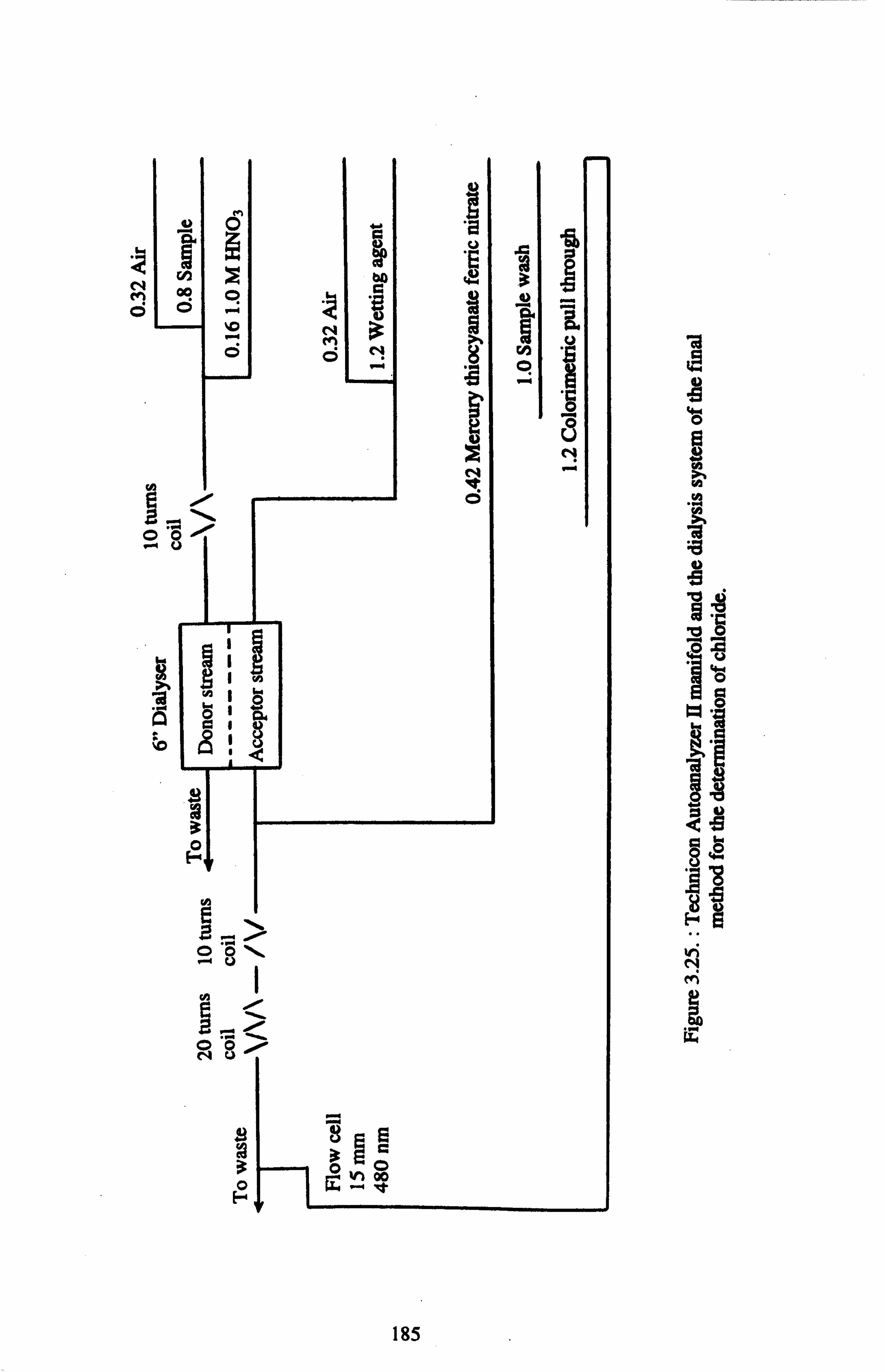
40

ä N OO

ýi ýý $ýý Ov

59

.., A

0o

1 ii

{#I o

ýä Q

3 E2

h

E a C

1114, Ü\

H

N Öý v 1000,

3 0 H

w O

as y H

'd O

aÖ

vi

a w

185

CHAPTER 4

INVESTIGATION OF GROUNDWATER QUALITY AND

SOILS IN THE ARDEER SITE

4.1. INTRODUCTION



and Nylon, and their associated acids, predominately Sulphuric and Nitric acids. It is

located at Stevenston, Ayrshire, Scotland (Map 4.1. ). A small part of the site was also

set aside as a licensed landfill facility. As a result of some of these activities localised

contamination has occurred. The particular interest of this study is the nitrogen

contamination of the groundwater associated with the areas of the site where the

groundwater has been contaminated by ammonium and nitrate.

1971 was the centenary year of the formation of the first British company to

manufacture nitro-glycerine-based explosives. Trading under various names and

subsequently becoming part of Imperial Chemical Industries Ltd. in 1926, the company

reverted to an earlier title of Nobel's Explosives Company Ltd., as a result of re-

organisation of a number of ICI divisions in 1971 (Nobel's Explosives Company

Limited Report, 1971).

In 1871, Alfred Nobel, backed by a group of Glasgow financiers, began the

preparation of the eighth of his seventeen world-wide commercial explosives

manufacturing plants at Ardeer on the Ayrshire coast in south west Scotland. The

selection of Ardeer as the site for the explosives manufacturing plant was made because

the vast expanse of sand dunes provided a barrier of isolation between the process plants

and neighbouring towns. The site also offered considerable space for expansion as

instanced by the original site of 100 acres growing to the present 2000 acres.

186

N GLASGOW "

PAISLEY "

Stevenston " 'ý ý- Ardeer site

" Irvine " KILMARNOCK

Irvine, Bay

Firth of Clyde

Ayr Bay " Ayr 012345 km

Map 4.1.: The location of the Ardeer site of Nobel Enterprises.

187

Production began in 1873 with "guhr dynamite", the first safe commercial

explosive to incorporate nitro-glycerine. From this beginning evolved a wide range of

nitro-glycerine-based explosives carefully formulated for a variety of uses in the mining,

quarrying and civil engineering industries.

Nobel's most fundamental invention was the detonator, a short copper tube

containing a minute quantity of mercury fulminate that could be handled safely and

which could be crimped on to the end of a length of safety fuse to provide a reliable

means of detonating nitro-glycerine to full effect even if it was unconfined. Nobel then

set about devising a safe method of manufacture for nitro-glycerine (known initially as

"blasting oil") and for its use in blasting and mining. Another of Nobel's basic contributions to explosives technology was the

absorption of nitro-glycerine in Keiselguhr, a diatomaceous earth, which could absorb

three times its weight of the "blasting oil, ' : this was the original "guhr dynamite" - first

manufactured at Ardeer in 1873. This moist crumbly mass could be cartridged in paper

and was the original powder blasting explosive. A third contribution by Nobel was the formulation and manufacture of

"blasting gelatine" formed by gelling 92 % of nitro-glycerine with 8% of collodion-type

nitrocotton. It is the most powerful commercial explosive, and provided a standard of

performance against which relative explosive strengths are measured. It was not

manufactured at Ardeer on any major scale until 1881 and only small quantities are

made, for it is too expensive for most modern purposes.

Nobel also formulated the smokeless powder ballistite, a military propellant

patented in 1887. Smokeless powders were part of the general development of weapons

which took place in the latter half of the nineteenth century. Before the end of the nineteenth century, plants were established at Ardeer for

the manufacture of soluble nitro-cellulose for gelatine blasting explosives and ballistite;

guncotton for manufacture of the Government propellant, Cordite (like ballistite a

gelatinised mixture of nitro-cellulose and nitro-glycerine); lead nitrate and picric acid

and many other products associated with explosive manufacture. By 1900, the original

100 acres of the Ardeer factory had grown to almost 500 acres and the numbers

employed had grown from 50 to 1300.

The passing of the Explosives Act in 1875 to control the manufacture, keeping, conveyance and importation of explosives for legitimate purposes brought the

188

Ardeer site and the many small explosives factories throughout the country under the

control of The Home Office. This regulation of manufacture was only one aspect of

government interest in high explosives. The bulk of industrial explosives manufacture in

the latter years of the nineteenth century was used in coal mining and, although high

explosives gradually replaced gunpowder in British mines, the loss of life in mining

accidents was still high.

In 1920, the name was changed to Nobel Industries Limited following more

acquisitions, including such famous names as Curtis & Harvey Limited (general

explosives business, running back over a century), Kynoch Limited (interests in

explosives, ammunition and metals), Eley Brothers Limited (specialists in shotgun

cartridges) and Bickford Smith & Co. Limited (safety fuse). At the time of the formation

of ICI in 1926, Nobel Industries Limited consisted of 36 subsidiary and 16 associated

companies throughout the world and was organised into four groups : explosives, metal

and ammunition, artificial leather, collodions and varnish, which formed the nuclei of

the Explosives, Metals, Leathercloth and Paints Divisions of ICI.

In 1928, the Ardeer site was still largely concerned in the manufacture of

products related closely to those established by Nobel, i. e. blasting explosives derived

from nitro-glycerine, propellants, guncotton nitro-cellulose, sulphuric acid and nitric

acid, refined glycerine. Between 1928 and the outbreak of the Second World War in

1939, many of the smaller factories inherited from Nobel Industries were closed down,

particularly those manufacturing blackpowder, safety fuse and detonators with the

transfer of these manufactures to the Ardeer site.

In 1933, the Division Research Department devised a new safety explosive - Hydrox which was a mixture of sodium nitrite and ammonium chloride giving on

initiation an evolution of gases from the decomposition of ammonium nitrite. Hydrox

itself became obsolete in 1955 but the technique had given rise to the production of

useful propellant devices during the 1939 - 1945 War and subsequently to the

production of pesticide smoke pellets, a manufacture which was carried on at Ardeer.

In 1934, the manufacture of Cordtex detonating fuse commenced, in which

TNT of the original Bickford Cordeau fuse was replaced by PETN (pentaerythritol

tetranitrate) and the original lead sheath replaced by textiles. This use of PETN was well

in advance of its later use as the base charge in detonators.

189

In propellant manufacture, the wet-mix method for Cordites, eliminating the

use of dry guncotton, led to an improvement in the safety of manufacture. The product

was used in anti-aircraft defence rockets and subsequently in engine starter cartridges

developed at Ardeer.

The end of 1914 - 1918 War left excess manufacturing capacity for nitro-

cellulose. A long programme of work commenced with the development of a safe

method of Kiering nitro-cellulose to give low viscosities suitable for industrial

application. The commercial process for the manufacture of methyl methacrylate

(Perspex) was originally developed at Ardeer in the thirties, although full scale

manufacture was transferred to another ICI site in Billingham.

During the 1939 - 1945 War most of the research effort was involved in work

directly connected with military requirements; in particular the development of

aeroplane engine starter cartridges, self-heating food cans, "plaster" blasting devices,

delay detonators for the RAF, the PIAT bomb (a shaped charge of NE 808 which was

insensitive to rifle bullets) and Stokes and Limpets for underwater work on ships. A new mechanical blasting explosives manufacturing unit was built in 1948

in which the explosives mixing, cartridging and packing operations were improved. A

subsequent unit, introduced in 1968, combines the mixing and cartridging processes in

one building, remotely controlled, introducing a further degree of safety into the

manufacture. Parallel to the work on the mechanisation of blasting explosives manufacture,

work was carried on in the more difficult mechanisation of detonator production. There

was, at Ardeer, one unit in which standard detonators were filled and pressed

automatically, a series of eight units in which electric detonators were assembled from

the three essential items, polyvinyl-chloride covered wire, fuseheads and filled standard

detonators, and a series of units in which fusehead assemblies themselves were made

automatically. Once again this led to improved safety and better labour utilisation.

Ardeer has also been involved in the production of slurry explosives and of

ammonium nitrate/fuel oil mixtures (ANFO) to meet modern blasting techniques. ICI

slurry explosives consists of a gelled aqueous solution of ammonium nitrate and sodium

nitrate with excess solids held in suspension with the sensitisers. ANFO is simply an

intimate mixture of ammonium nitrate (in absorbent prill form) and fuel oil. Both slurry

190

and ANFO explosives were easy and safe to handle, and had the advantage of

completely filling the borehole producing better rock coupling.

The manufacture of chemicals at Ardeer is not new and the production of

sulphuric acid, nitric acid and nitro-cellulose began early in the factory's life as

essentials of explosives manufacture. As a result of the continual search over in 1950's - 1960's for products to counter the fall in explosives requirements, many other chemical

manufactures were established on the Ardeer site. They include isopropyl nitrate,

industrial nitro-cellulose including plant to produce plasticised nitro-cellulose granules,

(particularly useful in the manufacture of the waterproofing lacquer applied to

transparent paper), silicone products (one of the largest manufacturing units in Western

Europe) supplied in the form of fluids, resins, greases and elastomers. These silicone

products found application as anti-foam agents, anti-stick treatments for paper and

baking pans, building sealants, lubricating fluids and greases, electrical resins, medical

specialities, cosmetics, mould release agents, polish additives, rubbers for cable

insulation and cloth coatings, water repellents for masonry, textiles and leather, adhesive

bonding agents and as the active component of the "Flexel" central heating system

manufactured and marketed by ICI.

A new organic chemicals complex was erected to produce a range of

chemicals based on maleic anhydride. The main uses of maleic anhydride were in

unsaturated polyester resins, flame retardant polymers, polyester surface coatings and insecticides. Downstream products of maleic anhydride manufacture include malic acid, fumaric acid, and tetrahydrophthalic anhydride (THPA) used in insecticides, fungicides

and in the manufacture of speciality resins. Sanction has been given for the erection of further plants to manufacture tetrahydrofuran (a solvent for elastomeric fibres),

butyrolactone (used in the synthesis of Vitamin E), hexahydrophthalic anhydride (a

curing agent for epoxy resins), chlorendic acid (a flame retardant) and "Viscofas", a

water soluble polymer which may be used in cosmetics, printing inks, and thickening

agents for carpet compositions.

In the last 28 years, further rundown in the manufacturing processes at the

site took place as a result of the decline in chemical manufacture and the decline in the

coal mining industry resulting in a greatly reduced demand for explosives (Tables 4.1.

and 4.2. ). This decline since the Second World War is shown by the number of

191

employee at the site (Table 4.3. ). The main process now at the site is the manufacture of

nitro-cellulose.

Table 4.1.: The decline in coal mining industry in Scotland as shown by the coal production (Pulford, 1999).

Year Coal production in Scotland

1913 1989

43.2 Mt (peak production) [15 % of UK output]. 6.4 Mt [6.0 % of UK output].

Table 4.2. : The decline in coal mining industry in Scotland as shown by the number of coal mines (Pulford, 1999).

Year Coal mines

1947 1993

250 pits 2 pits

Table 4.3. : The number of the employee in the Ardeer site (Craig, 1999).

Year Number of employee

1935 6000 1940 - 1945 8000* 1970 4000 1999 300

* Numbers of employee were not published during war time.

This large site with 128 years history of chemical manufacture and contamination is now requiring clean up with the objective of selling or redeveloping parts of the site.

This has required a program of soil survey and testing the buildings in the area, prior to

knocking down the buildings, removing the rubble, levelling the site, topsoiling and

revegetating. Small areas have been redeveloped for small business units or offices. They

have also carried out extensive borehole surveys to look for soil contamination.

Groundwater at the site is vulnerable to contamination due to the low CEC,

low clay content and high sand content which make the topsoil and subsoil likely to

leach contaminants. ICI has carried out an extensive groundwater monitoring program to

192

identify and trace the groundwater contamination in the site. Many wells were installed

for this purpose. They tend to install further boreholes in areas where contamination is

found. Therefore, they focused on the landfill area because of the contamination there.

Wells No. BH 5, BH 7, BH 9 and BH 10 were installed between the bank of River

Garnock and the high water line to check if the landfill area was leaching contaminants

to the River Garnock. In August, 1992, a large number of wells (wells No. SW I- SW

23 and TW 1- TW 11) were installed covering the whole site. In December, 1993, a

number of wells (wells No. SW 101 - SW 107) were installed covering the Nylon area. Finally, in November, 1995, more wells (wells No. TW 104 - TW 114) were installed to

extend cover of the landfill area.

The early surveys showed that groundwater is contaminated. Amin (1995)

investigated ammonium contamination of groundwater in the Nylon area. The current

study follows the work of Amin (1995) to look at the possibility of bioremediation

treatment of the contaminated groundwater in the Nylon area. The bioremediation

treatment being considered is by pumping well water to the surface, irrigating the

vegetation, and harvesting the vegetation (as vegetation such as ryegrass uses

ammonium and nitrate as a fertiliser before it leaches down in soil profile). In the

beginning the focus was mainly on ammonium contamination in the Nylon area, but

during the course of the current study high levels of ammonium and nitrate were found

in the groundwater of other areas. Therefore, the groundwater study was extended away from the Nylon area to the other areas.

In addition , in the current investigation, a soil survey was carried in selected

areas where soils have been remediated and vegetated to choose soil samples suitable

for experimental work.

Four areas were selected, IOP, H-Acid, Safety Fuse and Nylon and are shown

in Map 4.2. The description of each area is given below :

(a)- INTERMEDIATE OXIDATION PLANT QOP) AREA

Before the establishment of the IOP plant, the site was occupied by a number

of small stores. The bottoming for this building was probably slag from the adjacent former iron works. From 1950 to 1982, the IOP plant used ammonia as raw material and

oxidised it to manufacture nitric acid. It was demolished in 1993. The IOP area was

193

topsoiled to a depth of 15 cm in the Autumn of 1996. The topsoil used was light-

textured gravely sandy loam with low organic matter content (6.0 % ), friable

consistency and granular structure. Soil had a low water holding capacity and free

surface drainage. The soil was alkaline with no lime requirement. In addition, the soil

had low nitrogen status and there were no other major nutrient deficiencies. Moreover,

the soil had a moderate salinity status with no salinity problems.

(b)- H-ACID AREA:

From 1895 to 1970, this area was used for a series of acid mixing station

(nitric and sulphuric). The H-Acid plant was constructed in 1971 - 1976, and used for

manufacture from 1977 to 1992. The H-Acid plant manufactured Dye Stuff

Intermediates (H-Acid) and Monomer One (Bisphenol sulphone). The main products of

the H-Acid plant are presented in Figure 4.1. The plant was decontaminated and

demolished in 1993 and the area was topsoiled in the Autumn of 1993.

(c)- SAFETY FUSE AREA :

The Safety Fuse plant was built in 1935. It was used for the manufacture of

Safety Fuse from 1935 to 1991. Safety Fuse is a detonating cord with a Blackpowder

core. The Blackpowder was spun inside a Jute or cotton case, then covered in Bitumen

to make it waterproof. The Bitumen was replaced by plastic. Varnish was used as the

final covering. In addition, there was a Pesticidal Smoke Generator Plant which used

Hexachlorobenzene for the manufacture of pesticidal smoke generators from 1966 to

1990. There were also engineering workshops which used oils/greases and chlorinated

solvents to degrease equipment. The plant was decontaminated and demolished in 1995.

This area was topsoiled with 15 cm soil in the Autumn of 1996. The topsoil used was

the same as that used in the IOP area (Harris, 1999).

194

z 4-- ý

'ý d w¢

z x

Cs , S

V 4-4

0

Map 4.2.: The location of IOP, H-Acid, Safety Fuse, Nylon and landfill areas.

195

äDas

IQ SOsH

O 3D2H off

sus

jw

as

U-Acid O -Acid

(4-Amino-S-lydsazynaphtha1ene- (2-iydroxynaphthalene- 2,7-Disulphonic Acid) 6,8-Disulphonic Acid)

H 903H Ný

HOa3

OO

SWH 1033

O

SO, H

tr8 /laaward

(7-Aainanaphthalenue-1,3,6- (Naphthalene-1,3,6- Trieulphoaic Acid) TriaulpImic Acid)

Mb SO3H 0 02 SO3H

HO3 S SO3H HO3 S

JO O

S03 H

Koch Acid Nitrokoch Acid

(8-Aminonaphthalene-1.3,6- 18-Nitronaphthalene-1,3.6- Trisulphonic Acid) Trisulphonic Acid)

MOLECULAR FORMULA Cio H9 S2 NO7 CtoH8S2O7 CioH9S3NO9 CtoH&S3O9 CioH9S3N09 CIoH7S3NO>>

H-Acid G-Acid BNTS Azoguard Koch Acid Nitrokoch Acid

Figure 4.1.: The main products of the H-Acid plant.

196

(d)- NYLON AREA :

Before industrial use, up to the early years of this century, this area was a Golf course and Cricket pitch, and in the northern section, was mined for coal. The area

north of this area was extensively worked and a number of small canals were dug for

moving the coal, one of which remains and can still be seen as the Master Gott burn.

The ICI site was extended with the development of a plant for producing nylon. In 1964

the nylon factory construction work was started and it was completed in 1968. Ammonia

was brought in by rail for use in the nylon production plant and an associated nitric acid

plant. Nylon was produced for 14 years (1968 - 1981). The nylon plant was demolished

in 1981 leaving the nitric acid plant in operation. The ammonia storage was closed in

about 1984 and the nitric acid plant was closed in 1992. Demolition of these facilities

was carried out in 1993 (Amin, 1995). The site buildings were cleared leaving the

foundations in place and no further work was done. The main products of the Nylon

plant are illustrated in Figure 4.2.

From the groundwater and soil contamination point of view, the major

objectives of chapter 4 are :

1- To investigate the distribution and concentration of ammonium-N, nitrate-N and

other contaminants such as chloride, potassium, sodium, calcium, magnesium and

iron in the groundwater at the Ardeer site.

2- To investigate the sources of contamination and to evaluate the impact of the

industrial activity on the groundwater quality at the site.

3- To evaluate the groundwater quality parameters and their seasonal variations over a

period of time.

4- To characterise the four selected areas at the site to evaluate the soil contamination

due to toxic metals, consequently to select suitable soils for nitrification and plant

growth studies.

197

CD W

J 0- 2 W

F-- z

CL Z O

Z

}- Zw LLJ %

crS Zý0

m1Z Qr ui

Z tz- 0012

of ---ýº g [°1___ - CL Ya a-

Z

öäo° z¢z

ai O

Ü

1a 'O

0

198


SITE DESCRIPTION :

The Ardeer site of Nobel Enterprises is located at Stevenston, Ayrshire,

Scotland. At the northern edge of this site there is a railway line and just across the

railway line there is the Master Gott burn. This site has been used for the manufacture of

a range of chemicals and explosives such as Nitro-cellulose, Nitro-glycerine, Dyestuffs

and Nylon, and their associated acids, predominately Sulphuric and Nitric acids. A small

part of the site was also set aside as a licensed landfill facility. The site is shown in Map

4.3.

4.2.1. WATER QUALITY PARAMETERS

4.2.1.1. WATER SAMPLING

The water samples were collected for analysis from the suspected areas. The

locations of the sampling points for collecting the water samples are shown in Map 4.3.

and illustrated in Tables 4.4. and 4.5.

199

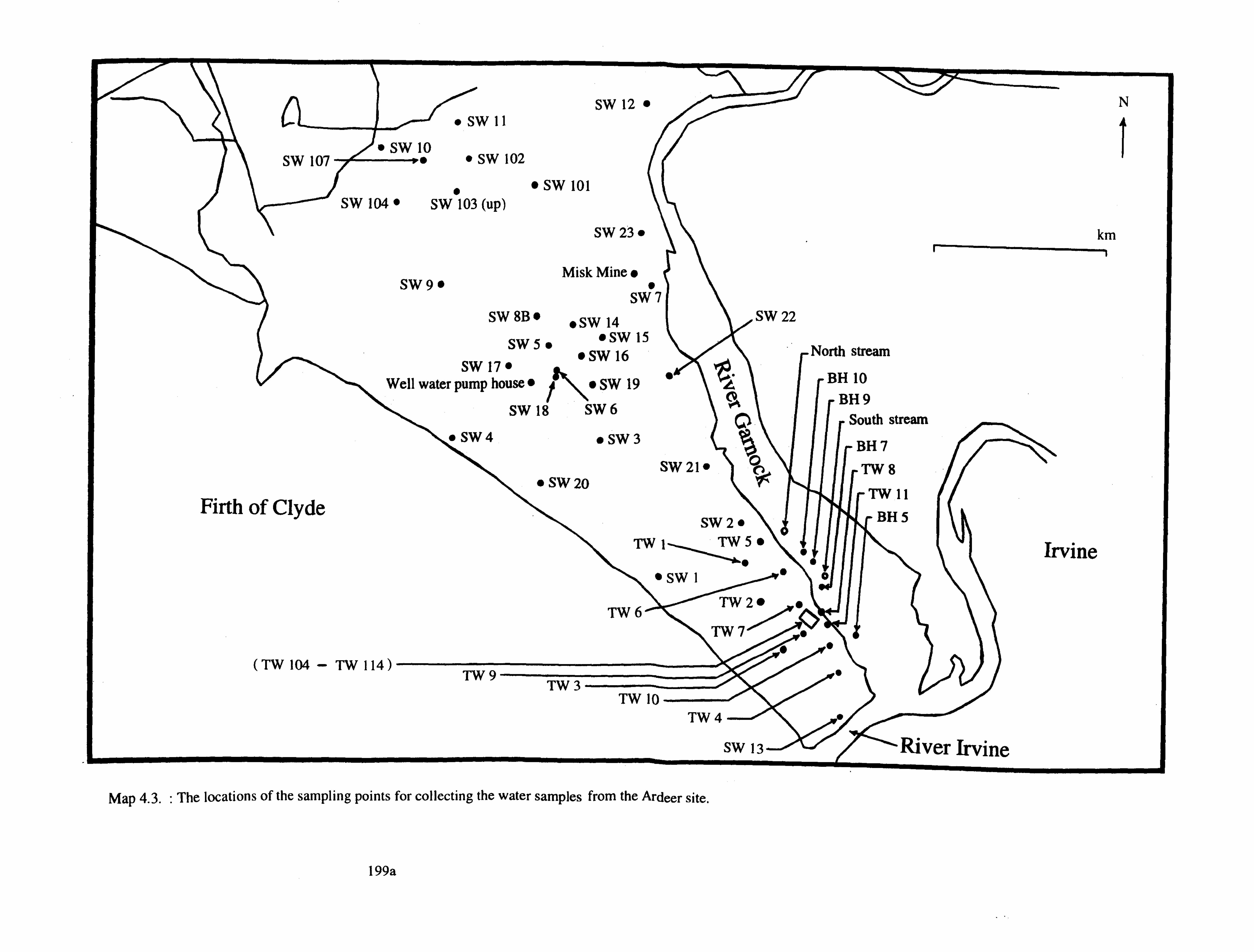
"SW11

ýSW10 SW 107 SW 102

0 SW 101 SW 104 " SW 103 (up)

SW 12 "

SW 23"

Misk Mine " SW9" "

SW 7 SW 8B "" SW 14 SW 22

SW5" "SW15

SW 17 " "SW16

Well water pump house "O SW 19

SW18 SW6

SW4 "SW3

SW 21" 0 SW20

Firth of Clyde

(TW 104 - TW 114) , 1, W9-

TW 3

SW2" TWIG TW5" N

N" sw i"

TWý, %', "

TW7ýý/

TW 10 TW4---/

SW 13

km I -I

Irvine

River Irvine mmý

i

Map 4.3. : The locations of the sampling points for collecting the water samples from the Ardeer site.

North stream

BH 10 BH 9

South stream

BH 7 TW 8

TW11

rBH5

199a

Table 4.4. : Locations of the sampling points of the groundwater monitoring wells.

Well No. Location

SW 1 Beside Long Sea Pipeline (LSP) [site effluent discharge] pumping station.

SW 2 Wharf road on landward side. SW 3 Outside Explosive Building in Subfactory "P" (PZ2), through

the cutting. SW 4 North of mix - pak, near shore magazines. SW 5 Building 400 compound. SW 6 Silver spoon. SW 7 Cordtex behind Explosive Building in Subfactory "B"

(BX 101). SW 8B Intermediate Oxidation Plant (IOP) [Nitric acid] across from

mining chemicals. SW 9 Large car park outside gate. SW 10 Nylon site old tanker area. SW 11 Nylon site (fuel area). SW 12 Garnock west between Explosive Building in Subfactory

"WP" (WPP2) and Explosive Building in Subfactory "WP" (WPP3).

SW 13 Shore front (Out of gate at point). SW 14 Organic General Purpose Unit (OGPU) yard. SW 15 Detonators between Explosive Building Subfactory "T" (TO1)

and Explosive Building Subfactory "T" (TO3). SW 16 In front of the sulphur shed. SW 17 Between Factory Warehouse/Store (Complex A) and the

medical centre. SW 18 Auto - nitration at Nitro-cellulose (NC) plant. SW 19 Grassy area at Assembly Building (P500). SW 20 Shore front beside Factory Magazine (CM 12). SW 21 At Garnock side of Silicones road. SW 22 Detonators at Explosive Building in Subfactory "D" (DV30). SW 23 Misk plasting at bottom of Explosive Building in Subfactory

"T" (TA 12) road. SW 101 Blackpowder. SW 102 Nylon site contractors area. SW 103 (upper) Nylon site cooling towers. SW 103 (lower) Nylon site cooling towers. SW 104 Nylon site near Ardeer Properties Ltd. (APL) land. SW 107 Nylon site - North end. Tw 1 Wharf road.

2 Outside mound of Explosive Building in Subfactory "M" (MG6).

200


Well No. Location

TW 3 Near burning station on Wharf road. TW 4 Short front out of point gate.

Misk Mine* 229135,640715. Well water * Beside Nitro-cellulose (NC) plant. pump house

* Misk Mine and Well water pump house are open shafts with water at ground level, depth unknown.

Table 4.5. : Location of the sampling points of the landfill groundwater monitoring wells.

Well No. Location

TW 5 Landfill area. TW 6 Landfill area. TW 7 Landfill area. TW 8 Landfill area. TW 9 Landfill area. TW 10 Landfill area. TW 11 Landfill area. TW 104 Landfill area. TW 105 Landfill area. TW 106 Landfill area. TW 107 Landfill area. TW 108 Landfill area. TW 109 Landfill area. TW 110 Landfill area. TW 111 Landfill area. TW 112 Landfill area. TW 113 Landfill area. TW 114 Landfill area. BH 5 Landfill area. BH 7 Landfill area. BH 9 Landfill area. BH 10 Landfill area.

North (Silicon) stream* Landfill area. South (Wharf) stream* Landfill area.

North (Silicon) stream and South (Wharf) stream are streams leaching from the landfill area at ground level.

201

PROCEDURE FOR SAMPLING THE GROUNDWATER MONITORING

WELLS

The water samples were obtained from 3" inch diameter wells down to a

depth of a 20 meters using a submersible pump powered by a 12 volt van battery. An

Eijkelkamp Agrisearch Equipment (Van Walt Ltd., Prestwick Lane, Grayswood,

Haslemere, Surrey GU27 2DU. ) gigant submersible pump was used with a whale

submersible in-line pump to obtain the necessary lift (Figure 4.3. ).

e 14

.e s

a H

H ýa

aý 14 {a as HH

%D co 00

.

`" '

"N 'O , -1 " ION"

to fý

3Ö

Z

('r) "W -r i. Ch c: to 0

lu -% H in C.

mbrI --4 CO 4380 A-8 34) 0040

O

r1

m 'd

8 äßo'-,

öýýöw +3 0 rq

CO 4J äo40 3

64 -V4 % 9%4

y8 ýý Co O

N ý-i

ü

3 ä

a u c c

u

u

.c GA GA "Ci

R

ä

a aý .c aý

.a a u

cri

w boo w

202

The submersible pump was unwound and lowered into the well until it

reached the bottom and then it was raised about one metre. The pump outlet was inserted into a waste drum and the pump terminals were connected to the battery and

switched on. The required volume of the purge water was pumped out. The purging was continued until the pH, temperature and conductivity of the

water had stabilised (two consecutive values within 10 %). The readings were recorded

on the sampling log sheet and the sample bottles were filled.

The pump was switched off and the tubing was removed slowly from the well

and the outside was washed with deionised water. Then the pump end was immersed in

deionised water and switched on to flush the inside of the pump and tubing. The pump

was switched off and disconnected from the battery.

Full decontamination of the equipment was carried out on return to the

laboratory as follows :

The pump and tubing were flushed with methanol, rinsed several times with tap water, then rinsed with deionised water. The pump and tubing were drained, dried

with paper towel and stored in a polythene bag until required again. The water samples were stored in the cold room at 2 °C until required for

analysis.

4.2.1.2. GROUND WATER SURVEYS

Four surveys were performed for the collection of the water samples for

analysis from the suspected areas. The description of each survey is illustrated as follows :

4.2.1.2.1. DESCRIPTION OF THE FIRST SURVEY

This survey was performed in October and November, 1996. The sample description is presented in Table 4.6. The locations of the sampling points are shown in

Map 4.3.

203

Table 4.6. : Groundwater sample description from the first survey.

Well No. Water level (Depth from ground level

in meters)

Total depth of well (meters)

Sampling date

SW 1 2.8 17.0 12/11/1996 SW 2 2.7 17.0 23/10/1996 SW 3 1.8 19.0 23/10/1996 SW 4 4.6 20.0 5/11/1996 SW5 3.3 19.0 22/11/1996 SW7 1.1 17.0 28/10/1996 SW 9 3.4 14.0 22/11/1996 SW 11 4.0 7.0 23 / 10 / 1996 SW 12 3.2 7.0 28 / 10 / 1996 SW13 3.8 15.0 21/10/1996 SW15 1.1 16.0 21/11/1996 SW17 3.1 20.0 12/11/1996 SW19 1.6 18.0 1/11/1996 SW 20 3.0 21.0 5/11/1996 SW21 1.8 16.0 12/11/1996 SW 22 1.6 11.0 21/10/1996 SW23 1.4 9.0 1/11/1996 SW 101 1.9 9.0 1/11/1996 SW 103 (upper) 1.4 11.0 7/11/1996 SW 103 (lower) 5.5 > 20.0 7/11/1996 SW 104 1.7 11.0 22/11/1996 TW4 3.2 16.0 21/10/1996

Misk Mine 7/11/1996 Well water 5/11/1996 pump house

4.2.1.2.2. DESCRIPTION OF THE SECOND SURVEY

This survey was performed in March and April, 1997. The sample description

is presented in Table 4.7. The locations of the sampling points are shown in Map 4.3.

204

Table 4.7. : Groundwater sample description from the second survey.


in metres

Total depth of well (metres)

Sampling date

TW 5 3.7 6.0 2/4/ 1997 TW 6 4.1 6.0 2/4/ 1997 TW 7 4.3 6.0 19 /3/ 1997 TW 8 3.8 10.0 20 /3/ 1997 TW 9 3.3 6.0 24 /3/ 1997 TW 10 2.4 6.0 24 /3/ 1997 TW 11 2.1 5.0 24 /3/ 1997 TW 104 4.5 8.0 20 /3/ 1997 TW 105 4.1 8.0 20 /3/ 1997 TW 106 3.8 8.0 18 /3/ 1997 TW 107 4.1 8.0 19 /3/ 1997 TW108 4.1 8.0 19/3/1997 TW 109 4.6 8.0 20 /3/ 1997 TW 110 4.6 8.0 20 /3/ 1997 TW 111 4.4 8.0 20 /3/ 1997 TW 112 3.2 8.0 20 /3/ 1997 TW 113 4.4 8.0 24 /3/ 1997 TW 114 5.0 9.0 24 /3/ 1997 BH 5 0.0 5.0 1/4/ 1997 BH 7 0.0 6.0 1/4/1997 BH9 0.0 6.0 2/4/ 1997 BH 10 0.0 5.0 2/4/1997

North (Silicon) 1/4/ 1997 stream South (Wharf) 1/4/ 1997 stream

4.2.1.2.3. DESCRIPTION OF THE THIRD SURVEY

This survey was performed in April, May and June, 1997. The sample description is presented in Table 4.8. The locations of the sampling points are shown in

Map 4.3.

205

Table 4.8. : Groundwater sample description from the third survey.


in metres


Sampling date

SW 1 2.8 17.0 16/4/ 1997 SW2 2.7 17.0 30/4/ 1997 SW 3 1.8 19.0 16/4/ 1997 SW4 4.6 20.0 17/4/ 1997 SW5 3.3 19.0 1/5/1997 SW6 2.3 8.0 5/6/1997 SW 7 1.1 17.0 9/4/ 1997 SW 8B 1.3 14.0 16/5/1997 SW9 3.4 14.0 15/5/1997 SW 10 3.1 10.0 1/5/1997 SW 11 4.0 7.0 16/4/1997 SW 12 3.2 7.0 9/4/ 1997 SW13 3.8 15.0 2/5/1997 SW 14 1.7 10.0 16/5/ 1997 SW 15 1.1 16.0 9/4/ 1997 SW 16 2.0 15.0 15/5/1997 SW 17 3.1 20.0 22 /5/ 1997 SW 18 2.8 19.0 9/6/1997 SW 19 1.6 18.0 15/5/ 1997 SW 20 3.0 21.0 16 /5/ 1997 SW22 1.6 11.0 16/4/1997 SW 23 1.4 9.0 9/4/ 1997 SW 101 1.9 9.0 30 /4/ 1997 SW 102 2.6 10.0 22 /4/ 1997 SW 103 (upper) 1.4 11.0 22 /4/ 1997 SW 103 (lower) 5.5 > 20.0 22 /4/ 1997 SW 104 1.7 11.0 22 /4/ 1997 SW 107 1.6 11.0 17 /4/ 1997 TW 1 1.4 15.0 30/4/ 1997 TW 2 3.1 11.0 16/5/ 1997 TW3 1.2 13.0 2/5/1997 TW4 3.2 16.0 15/5/1997

Misk Mine 17 /4/ 1997 Well water 4/6/ 1997 pump house

206

4.2.1.2.4. DESCRIPTION OF THE FOURTH SURVEY

This survey was performed in June and August, 1997. The sample

description is presented in Table 4.9. The locations of the sampling points are shown in

Map 4.3.

Table 4.9. : Groundwater sample description from the fourth survey.

Well No. Water level (Depth from ground level in metres


Sampling date

SW 2 2.7 17.0 25 /6/ 1997 SW 3 1.8 19.0 24/6/ 1997 SW 4 4: 6 20.0 24/6/1997 SW5 3.3 19.0 28/8/1997 SW 8B 1.3 14.0 23 /6/ 1997 SW9 3.4 14.0 23/6/1997 SW 10 3.1 10.0 23 /6/ 1997 sw 11 4.0 7.0 19/8/ 1997 SW 17 3.1 20.0 24 /6/ 1997 SW 101 1.9 9.0 19/8/ 1997 SW 102 2.6 10.0 23 /6/ 1997 SW 103 (upper) 1.4 11.0 23 /6/ 1997 SW 103 (lower) 5.5 > 20.0 23 /6/ 1997 SW 104 1.7 11.0 19/8/ 1997 SW 107 1.6 11.0 11/8/1997 TW 1 1.4 15.0 11/8/1997 TW2 3.1 11.0 25/6/1997 TW3 1.2 13.0 11/8/1997

4.2.1.3. CHEMICAL ANALYSIS OF THE GROUNDWATER SAMPLES

The following analysis were carried out :

pH, EC, soluble ions such as NH4-N, N03-N, N02-N and Cl and total metals (calcium, magnesium, sodium, potassium and iron).

Some of the water samples contained suspended material. For analysis of the

solution ions the samples were filtered through a glass microfibre filter and for the

determination of the total metals the samples were digested in HNO3 acid.

207

The following water samples needed filtration and digestion :

Wells No. SW 3, SW 5, SW 7, SW 8B, SW 9, SW 10, SW 11, SW 15, SW

16, SW 18, SW 19, SW 22, SW 101, SW 102, SW 103 (lower), SW 104, SW 107, TW

1, TW 2, TW 4, Misk Mine, TW 5, TW 6, TW 8, TW 10, TW 11, TW 104, TW 105,

TW 106, TW 109, TW 110, TW 111, TW 112, TW 113, TW 114, BH 5, BH 7, BH9

and BH 10; and the North (Silicon) stream and South (Wharf) stream.

The remainder of the water samples did not require filtration or digestion.

The determination of NH4-N, N03-N and N02-N was the first analysis to be

carried out since there may be bacterial activity on these soluble ions if they were left for

1 to 2 weeks without analysis.

(a)- FILTRATION PROCEDURE :

This process was carried out to remove the suspended material from some of

the water samples.

The water sample was shaken well and then filtered under vacuum through a 47.0 mm diameter grade GF/C glass microfibre filter (Whatman) and the filtrate was

collected in a 28 ml universal bottle. Then the filtrate was transferred to 100 ml plastic

bottle for storage.

(b)- DIGESTION PROCEDURE :

This process was carried out to dissolve the undissolved metals such as

calcium, magnesium, sodium, potassium and iron which were present in some of the

water samples as a precipitate.

The digestion process was carried out in the acid resistant fume cupboard. Large glass funnels (24.5 cm diameter) were inverted over the sample beakers and

connected to a water powered vacuum pump to remove HNO3 acid fumes and the

water vacuuming was switched fully on to help in removing the HNO3 acid fumes.

The water sample was shaken well and then 25 ml was placed in 100 ml beaker, 2.5 ml concentrated HNO3 acid was added and the contents were swirled by a

glass rod. The beaker was placed on a hot plate for 45 minutes at 120 °C to digest and to

evaporate about half of the sample volume. The beaker was left to cool to room

208

temperature and the contents were transferred to a 25 ml volumetric flask with deionised water and the volume was made up to the mark with deionised water. The

digested sample was transferred to 60 ml glass bottle for storage. In the case of the

determination of sodium and potassium, the digested sample was kept in a plastic bottle

since the sodium present in the walls of the glass bottle may be dissolved and

contaminate the water sample.

The electrical conductivity (EC) was measured using a Jenway 4070

conductivity meter as in section 2.6.

The pH was measured by a combined glass / reference electrode as in section 2.4.

Ammonium was determined using automated colorimetry with gas phase dialysis as described in section 3.3.2.2.3. using a standard series 0.0 to 10 mg /1 NH4-N

in deionised water.

Nitrate was determined using automated colorimetry with liquid liquid

dialysis as described in section 3.3.3.2.2. using a standard series 0.0 to 10 mg /1 N03-N

in deionised water.

Nitrite was determined using automated colorimetry with liquid liquid

dialysis as described in section 3.3.3.2.2. using a standard series 0.0 to 1.0 mg ii N02-N

in deionised water.

Chloride was determined using automated colorimetry with liquid liquid

dialysis as described in section 3.3.3.2.4. using a standard series 0.0 to 100 mg it Cl in

deionised water.

Potassium was determined by the Flame photometer as described in section 2.11.3. It was determined in the undigested samples using a standard series 0.0 to 5.0

mg K' /1 in deionised water and in the digested samples using a standard series 0.0 to

5.0 mg K+ /1 in 10 % HNO3 solution.

Sodium was determined by the Flame photometer as described in section

2.11.4. It was determined in the undigested samples using a standard series 0.0 to 2.5

mg Na+ /1 in deionised water and in the digested samples using a standard series 0.0 to

2.5 mg Na+ /1 in 10 % HNO3 solution.

Iron was determined by the Atomic Absorption Spectrophotometer as

described in section 2.12.1. It was determined in the undigested samples using a

209

standard series 0.0 to 5.0 mg Fe /1 in deionised water and in the digested samples using a

standard series 0.0 to 5.0 mg Fe /1 in 10 % HNO3 solution.

Calcium was determined by the Atomic Absorption Spectrophotometer as described in section 2.11.5. It was determined in the undigested samples using a

standard series 0.0 to 5.0 mg Ca /1 in deionised water containing 10 % vol. /vol. of 3%

wt. /vol. SrC12.6H20 solution. It was determined in the digested samples using a

standard series 0.0 to 5.0 mg Ca /1 in 10 % HNO3 solution containing 10 % vol. /vol. of

3% wt. /vol. SrC12.6H20 solution.

Magnesium was determined by the Atomic Absorption Spectrophotometer

as described in section 2.11.6. It was determined in the undigested samples using a

standard series 0.0 to 0.5 mg Mg /1 in deionised containing 10 % vol. /vol. of 3%

wt. /vol. SrC12.6H20 solution. It was determined in the digested samples using a

standard series 0.0 to 0.5 mg Mg /1 in 10 % HNO3 solution containing 10 % vol. /vol. of 3% wt. /vol. SrC12.6H20 solution.

210

4.2.2. CHARACTERISATION OF THE SOILS

4.2.2.1. SOIL SAMPLING

The soil samples were collected from 4 candidate areas for analysis on 5/ 8/

1997. The profile was cleaned to get definite layers. The soil sample was collected from

each layer separately. The soil sample was taken from the bottom layer and up to the top

layer to avoid the contamination of the layers in case if the soil sample was taken from

the top layer first. Each layer was described according to its contents, texture and colour.

The vegetation around each hole was described. The soil samples were brought to the

laboratory in labelled plastic bags as soon as possible and kept in the cold room at 2 °C

until required for the analysis.


Soil samples were collected from 5 sites in the IOP area. The locations of the

sampling points are shown in Map 4.4. The sample description is given below :

SITE No. I:

Vegetation : White clover and very poor grass (about 50 % coverage).

Depth (cm)

0-14 : Topsoil, grey compacted clay.

14 - 24 : Brown compacted and sandier.

> 24 : Building rubble, concrete, brick and sand. Very hard and compacted.

Sample No. 1a: 0- 14

Sample No. 1b: 14 - 24

Sample No. 1c: > 24

SITE No. 2:

Vegetation : Predominately white clover and some grass.

211

Depth (cm)

0-12 : Topsoil.

12 - 33 : Soil and ash mixture.

33 - 40 : Ash.

40 - 50 : Sandy, stony subsoil and ash.


Sample No. 2b: 12 - 33

Sample No. 2c: 33 - 40

Sample No. 2d: 40 - 50

SITE No. 3:

Vegetation : White clover and grass (about 78 % coverage, mostly clover).

Depth (cm)

0-8 : Topsoil.

>8: Soil and ash.

Sample No. 3a: 0-8

SITE No. 4:

Vegetation : Very poor grass (less than 50 % coverage).

Depth (cm)

0-6 : Topsoil and very compacted.

>6: Mixture of soil containing stony rubble.

Sample No. 4a: 0-6

SITE No. 5:

Vegetation : Bare.

212

Depth (cm)

0-15 : Topsoil, sandy.

> 15 Building rubble.



The soil samples were collected from 4 sites in the H-Acid area. The

locations of the sampling points are shown in Map 4.5. The sample description is given

below :

SITE No. 6:

Vegetation : White clover mixed with grass (about 50 %: 50 % mix, full coverage).

Depth (cm)

0-17 : Topsoil.

> 17 : Sandy, very stony topsoil and building rubble.


SITE No. 7:


Depth (cm)

0-11 Topsoil.

> 11 : Building rubble.


SITE No. 8:

Vegetation : Better than those of sites No. 6 and 7.

213

Depth (cm)

0-22 : Topsoil.

> 22 : Loose sandy soil, very few stones, roots throughout.


SITE No. 9:


Depth (cm)

0-15 : Topsoil.

> 15 Sand, concrete and building rubble.

Sample No. 9a0- 15

Sample No. 9b: > 15 ( most of the stone has been removed from the sample).


The soil samples were collected from 4 sites in the Safety Fuse area. The

locations of the sampling points are shown in Map 4.6. The sample description is given below :

SITE No. 10:

Vegetation : White clover and very poor grass (less than 50 % coverage).

Depth (cm)

0-23 : Topsoil, sandy and slightly compacted.

23 - 55 : Banded sand.

> 55 : Yellow sand.

Sample No. 10 a: 0- 23

Sample No. 10 b 23 - 55

Sample No. 10 c> 55

214

S1TE No. 11 :

Vegetation : Mostly white clover and poor grass (80 % coverage).

Depth (cm)

0-18 : Topsoil, sandy loam.

18 - 40 : Yellow sand.

Sample No. Il a: 0-18

STTE No. 12:

Vegetation : Predominately white clover with poor grass (50 - 80 % coverage).

Depth (cm)

0-20 : Topsoil, compacted.

> 20 : Asphalt rubble.


SITE No. 13:

Vegetation : Very poor grass and very little white clover (less than 50 % coverage).

Depth (cm)

0-20 : Topsoil, sandy loam.

20 - 50 : Yellow sand.


Sample No. 13 b 20 - 50


The soil samples were collected from 4 sites in the Nylon area. The locations

of the sampling points are shown in Map 4.7. The sample description is given below :

215

STTE No. 14:

Vegetation : Thick grass.

Depth (cm)

0-30 : Topsoil, sand.

> 30 : Concrete and building rubble.


SITE No. 15:

Vegetation : Grass (gorse and broom).

Depth (cm)

0-2 Mat of litter.

2-40 : Disturbed sand.


SHE No. 16:

Vegetation : Very short grass, moss and trefoil.

Depth (cm)

0-28 : Disturbed sand and stone.


SITE No. 17:

Vegetation : Very short grass, moss, trefoil.

216

Depth (cm)

0-2 : Root and litter mat.

0-14 : A-horizon. Naturally developing topsoil. Slightly stony sand.

14 - 47 : Possibly disturbed to this depth.

> 47 Yellow sand.


Sample No. 17 b: 14 - 47

217

i

kf)

Z

/47 i r\

\\p

\z

\\ \\ \' \

.\\ý

\. '

05

v C5 z N

S.. \

S.

-- r'

N

O

z

1 ý; \\ Map 4.4. : The locations of the sampling points for collecting the soil samples

from the IOP area.

218

N

N N, /

N, N,

Tanks

IXN \ý

///

/ //

1 ýý \\\"O

// // // /" EX H-ACID SITE

0 0.

N, N,

\// Metres

N, IN 0 50 "I N,

Map 4.5.: The locations of the sampling points for collecting the soil samples from the H-Acid area.

219

.............. .....

Metres

Site No. 12 "

ýýý " Site No. 13

t .............................. ýý ...... ....................................................

Site No. 11 "

il

ii" Site No. 10

'I

rVQflvr

0 50

ö

ö

O

/

``ý l

Map 4.6.: The locations of the sampling points for collecting the soil samples from the Safety Fuse area.

220

1r site north

i=ce FUEL a

MR iDW R6

Sl? ITMý95 ý 'MS1E TMK NO/LRIITOR

^ NTR1C N2

AOD

Site No. 14 "

51 Site No. 15 .

" Site No. 17

-' ýonc Sao LoOU coa, EG POND

-ý o Cj c

0 50 10e.

metres

0

Site No. 16 0

Map 4.7.: The locations of the sampling points for collecting the soil samples from the Nylon area.

221

4.2.2.2. PREPARATION OF THE SOIL SAMPLES FOR PHYSICAL AND

CHEMICAL ANALYSIS

Each soil sample was spread on a clean plastic sheet and mixed well. Three

quarters of the sample was stored in the cold room at 2 °C as a reserve of untreated

material. The remaining quarter was prepared for analysis. The soil samples were air

dried just enough to pass through a2 mm stainless steel sieve. The sieved material was

further split in two subsamples (fresh and air dried). The fresh soil samples were kept in

the cold room at 2 °C until required for the determination of moisture content, organic

matter by loss on ignition, ammonium and nitrate. The remaining subsample was spread

on a clean plastic sheet and left at room temperature until completely air dried. The

dried soil samples were kept in a dry place until required for the determination of pH,

electrical conductivity, potassium and phosphorus.

Approximately 50 g of air dried soil sample was grinded with a mortar and

pestle to break the aggregates and to get the actual particle size. The mortar and pestle

were cleaned between every soil sample by scrubbing with acid washed sand and rinsed

with deionised water. The ground soil was stored in self sealing plastic bag in a dry

place until digestion for the determination of the total metals. The grinding was carried

out in the fume cupboard since it produces dust.

4.2.2.3. PHYSICAL AND CHEMICAL ANALYSIS OF THE SOIL SAMPLES

Moisture content was determined as described in section 2.7.

Organic matter (LOI) was determined as described in section 2.8.

pH was measured by a combined glass / reference electrode as in section 2.3.

The electrical conductivity was measured using a Jenway 4070 conductivity

meter as described in section 2.5.

The soil samples were digested as described in section 2.20. Copper, nickel,

zinc, chromium, cadmium and lead were determined in the soil digest by the Atomic

Absorption Spectrophotometer as described in sections 2.12.2., 2.12.3., 2.12.4., 2.12.5.,

2.12.6. and 2.12.7.

Cadmium, chromium, nickel, zinc, lead, boron, barium, manganese,

magnesium and potassium were determined in the soil digest by the Inductively Coupled

222

Plasma (ICP) Spectroscopy as described in section 2.14. at Nobel Enterprises, Ardeer

site. Inorganic nitrogen was extracted from the soil samples as described in

section 2.17. NH4-N was determined in the filtrate as described in section 3.1.3.2. using

a standard series 0.0 to 1.0 mg /1 NH4-N in 0.5 M K2SO4 solution. N03-N was

determined in the filtrate as described in section 2.11.1.3. using a standard series 0.0 to

1.0 mg /1 N03-N in 0.5 M K2SO4 solution. Phosphorus was extracted from the soil samples as described in section 2.18.

Phosphorus was determined in the neutralised soil extract as described in section 2.11.2.

using a standard series 0.0 to 1.0 mg P /1 in 0.5 M Na2SO4.

Potassium was extracted from the soil samples as described in section 2.19.

Potassium was determined in the filtrate by the Flame photometer as described in

section 2.11.3. using a standard series 0.0,5,10,15 and 20 mg K+ /1 in 1M NH4NO3

solution.

223

4.3. RESULTS AND DISCUSSION


4.3.1.1. PH

The seasonal variations of the pH in the groundwater monitoring wells are

presented in Table 4.10. The chemical composition of the landfill groundwater

monitoring wells (Spring, 1997) is shown in Table 4.11. As can be seen, the majority of

the wells had pH in the range from 6.1 to 8.3 but some wells were acidic (pH below

4.3). The North stream had a slightly higher pH (7.7) and the South stream had an acidic

pH (3.3). The high pH in the Nylon area could be due to ammonia spillage in the Nylon

area since ammonia was used in the nylon production plant and an associated nitric acid

plant and this is evidenced by the high pH of wells No. SW 10, SW 104, SW 102, SW

103 (upper) and SW 107 [pH in the range from 7.3 - 8.4]. The acidic pH could be due to

acid leakage as use of strong acids was widespread at the site.

In the majority of the wells, there were no great seasonal variations of the pH

except wells No. SW 3 and TW 2 which had a variable pH.

4.3.1.2. AMMONIUM-N

The seasonal variations of ammonium-N in the groundwater monitoring

wells are given in Table 4.12. The chemical composition of the landfill groundwater

monitoring wells (Spring, 1997) is shown in Table 4.11. It was noticed that the natural

background level of ammonium was < 1.0 mg NH4-N /1 at the site. About one third of

the wells were contaminated with ammonium particularly wells No. SW 11, SW 14, SW

16, SW 107, TW 8, TW 104, TW 105, TW 106, TW 112 and TW 114. Well No. SW 15

was extremely contaminated. The North stream was not contaminated with ammonium

but the South stream was contaminated.

There were three areas (hot spots) at the site with ammonium contamination,

these areas were quite localised. In the first hot spot, one well (well No. SW 14) had a

moderate level of ammonium, one well (well No. SW 16) had high level of ammonium

and the main well was well No. SW 15 which was enormously contaminated with

ammonium. However, there were a number of wells (wells No. SW 14, SW 5, SW 6,

224

SW 8B, SW 17 - SW 19 and well water pump house) which are close to it and were not

high in ammonium. Ammonium level increases with the depth of the wells (see Tables

4.7. and 4.8. ) of the first hot spot, particularly in wells No. SW 15 and SW 16. In

addition, the high and very high levels of ammonium occurred in wells with higher

water levels in the range from 1.1 - 2.0 metres below ground surface (see Table 4.8. ) and

this may be contribute to the ammonium level in the drainage water. In the second hot

spot, in the Nylon area, there were wells No. SW 11 and SW 107. The high levels of

ammonium in these wells may be due to ammonia spillage in the Nylon area since

ammonia was used in the nylon production plant and an associated nitric acid. In the

third hot spot, wells No. TW 8, TW 104 - TW 106, TW 112 and TW 114 showed

contamination. In the majority of the wells, there were no great seasonal variations of

ammonium level except wells No. SW 11, SW 15 and SW 107 which had variable

levels of ammonium.

4.3.1.3. NITRATE-N

The seasonal variations of nitrate-N in the groundwater monitoring wells are

summarised in Table 4.13. The chemical composition of the landfill groundwater

monitoring wells (Spring, 1997) is shown in Table 4.11. It was observed that the natural

background level of nitrate was < 1.0 mg N03-N /1 at the site. About half of the wells

were contaminated with nitrate particularly wells No. SW 2, SW 3, SW 6, SW 11, SW

23, TW 2, BH 7 and BH 9. Wells No. SW 14 - SW 16 and SW 18 were extremely

contaminated. The North stream was contaminated with nitrate but the South stream

was not contaminated.

There were two hot spots of nitrate at the site, the first hot spot includes

wells No. SW 3, SW 6, SW 14 - SW 16 and SW 18. The second hot spot includes wells

No. SW 2, TW 2, BH 7 and BH 9; and the North stream. The high nitrate levels could

be attributed to the spillage of nitric acid in the H-Acid area as evidenced by the high

levels of nitrate with low pH in wells No. SW 6, SW 14, SW 16 and SW 18. The nitrate

contamination was very closely localised. Although well No. SW 18 is very close to

well No. SW 6, it had a level of nitrate higher than that of well No. SW 6 and this could

be because well No. SW 18 is deeper than well No. SW 6 (see Table 4.8. ). By

225

comparing nitrate concentration in well No. SW 6 with that of well No. SW 18, there is

some evidence that nitrate increases with the depth of the well in the hot spot,

particularly in wells No. SW 15, SW 16 and SW 18 (see Table 4.8. ). Furthermore, the

high and very high levels of nitrate occurred in wells with high water levels in the range

from 1.1 - 2.8 metres below ground surface (see Table 4.8. ).

Of the all wells, there were more seasonal variations of nitrate level in about half of the wells particularly in wells No. SW 2 and SW 3 which had very variable

levels of nitrate and in wells No. SW 15 and SW 23 which had variable levels of nitrate.

Ammonium and nitrate were not necessarily found together as can be seen from wells

No. SW 6, SW 14, SW 18, SW 23 and TW 2.

4.3.1.4. NITRITE-N

The seasonal variations of nitrite-N in the groundwater monitoring wells are demonstrated in Table 4.14. The chemical composition of the landfill groundwater

monitoring wells (Spring, 1997) is shown in Table 4.11. As can be seen, the natural

background level of nitrite was < 0.1 mg N02-N /I at the site. Wells No. SW 11 and SW

18 were contaminated with nitrite. The North and South streams were not contaminated

with nitrite. Nitrite is unstable under acid conditions and would not be expected in

acidic groundwaters.

Regarding the seasonal variations of nitrite level, well No. SW 11 had a very

variable level of nitrite.

226

Table 4.10.: Seasonal variations of the pH in the groundwater monitoring wells.

Well No. Autumn 1996

Spring (1997)

Summer (1997)

SW 1 7.2 7.7 ---- SW 2 1.9 1.4 1.6 SW 3 4.3 7.9 7.6 SW 4 7.0 7.8 7.6 SW 5 7.0 7.2 7.6 SW 6 ---- 2.1 ---- SW 7 7.1 7.9 ---- SW 8B ---- 4.1 4.4 SW 9 7.1 8.2 8.0 SW 10 ---- 8.3 8.0 SW 11 6.7 6.5 5.1 SW 12 6.8 6.5 ---- SW 13 7.4 7.3 ---- SW 14 ---- 1.0 SW 15 7.2 7.6 ---- SW 16 ---- 3.8 ---- SW 17 7.6 7.8 7.8 SW 18 ---- 3.7 ---- SW 19 7.6 8.3 ---- SW 20 7.6 8.0 ---- SW 21 7.5 ---- ---- SW 22 7.5 8.2 ---- SW 23 7.4 7.9 ---- SW 101 7.2 7.4 7.5 SW 102 ---- 8.0 7.7 SW 103 (upper) 7.5 7.7 7.5 SW 103 (lower) 7.9 8.5 8.1 SW 104 7.3 8.2 8.1 SW 107 ---- 8.4 8.1 TW 1 ---- 7.7 7.8 TW 2 ---- 6.2 4.1 TW 3 ---- 7.6 7.7 TW 4 7.5 8.4 ----

Misk Mine 7.8 8.5 ---- Well water pump house 7.9 8.1 ----

---- No sample collected.

227

Table 4.11. : Chemical composition of the landfill groundwater monitoring wells (Spring, 1997).

Well No.

PH EC* (ms /cm

NH4-N (m /1

N03-N (m /1)

N02-N (Mg ) /1

Cl (Mg/1

TW 5 2.4 4.3 1.3 4.7 <0.1 54 TW 6 8.1 1.1 <0.1 <0.1 <0.1 54 TW 7 2.1 4.1 0.3 0.5 <0.1 678 TW 8 7.5 5.2 41.0 0.2 <0.1 1050 TW9 8.2 1.0 <0.1 0.2 <0.1 54 TW 10 8.3 1.2 <0.1 7.7 <0.1 141 TW 11 8.2 3.0 <0.1 8.0 <0.1 278 TW 104 2.4 4.4 21.0 0.1 < 0.1 680 TW 105 2.3 4.8 17.0 0.1 <0.1 1065 TW 106 2.3 7.7 58 4.0 <0.1 2208 TW 107 2.0 5.0 0.9 <0.1 <0.1 738 TW 108 1.5 15.0 1.9 2.9 <0.1 592 rw 109 8.2 2.9 <0.1 8.0 <0.1 332 TW 110 7.6 2.1 5.4 0.6 <0.1 295 TW 111 8.2 1.3 4.7 <0.1 <0.1 151 TW 112 2.3 5.0 19.3 0.8 <0.1 956 TW 113 8.1 2.1 <0.1 2.1 <0.1 109 TW 114 2.7 2.9 38.0 0.3 <0.1 142 BH 5 8.1 5.9 <0.1 0.1 <0.1 1997 BH7 7.2 36.0 <0.1 31.0 <0.1 10414 BH 9 7.5 36.0 <0.1 14.0 <0.1 9855 BH 10 7.9 13.3 <0.1 <0.1 <0.1 4827

North (Silicon) 7.7 45.0 <0.1 12.0 <0.1 13122 stream South (Wharf) 3.3 19.0 9.4 0.3 < 0.1 7468 stream

* EC = Electrical conductivity.

228

Table 4.11.: Continued.

Well No.

I K (Mg /1)

Na (m /1)

Ca

-(M g/1)

Mg (nig /1)

Fe m /l

TW5 2.5 41.3 460 104 506 TW 6 10.0 78 169 22.8 123 TW 7 40.0 46.3 178 16.0 34.5 TW 8 60 143 720 524 147 TW 9 35.0 133 73 6.6 < 0.05 TW 10 15.0 103 104 37.2 0.1 TW il 165 425 305 83 154 TW 104 275 188 190 106 290 TW 105 215 225 210 93 208 TW 106 110 115 435 208 462 TW 107 15.0 70 165 24.7 82 TW 108 20.0 90 190 40.2 235 TW 109 82 425 241 132 4.7 TW 110 42.5 169 227 69 24.5 TW 111 12.0 133 111 26.2 89 TW 112 100 103 221 177 335 TW 113 170 155 190 144 0.2 TW 114 20.0 109 234 79 124 BH 5 55 900 122 399 3.4 BH 7 180 5625 327 684 34.0 BH 9 210 5025 239 786 31.0 BH 10 115 3150 90 463 2.0

North (Silicon) 250 7100 265 896 0.9 stream South (Wharf) 185 2950 296 564 76 stream

229

Table 4.12.: Seasonal variations of ammonium-N (mg /1) in the groundwater monitoring wells.


Spring (1997)

Summer (1997)

SW 1 <0.1 <0.1 ---- SW 2 3.4 3.9 2.2 SW 3 <0.1 <0.1 <0.1 SW 4 < 0.1 < 0.1 <0.1 SW 5 < 0.1 <0.1 <0.1 SW 6 ---- 0.7 ---- SW 7 <0.1 <0.1 ---- SW 8B ---- 2.0 1.9 SW 9 < 0.1 <0.1 <0.1 SW 10 ---- <0.1 <0.1 SW 11 37.9 28.0 9.3 SW 12 <0.1 <0.1 ---- SW 13 <0.1 <0.1 ---- SW 14 ---- 17.8 ---- SW 15 7230 8090 ---- SW 16 ---- 117 ---- SW 17 <0.1 <0.1 <0.1 SW 18 ---- 5.1 ---- SW 19 <0.1 <0.1 ---- SW 20 < 0.1 <0.1 ---- SW 21 <0.1 ---- ---- SW 22 <0.1 <0.1 ---- SW 23 <0.1 <0.1 ---- SW 101 <0.1 <0.1 <0.1 SW 102 ---- <0.1 <0.1 SW 103 (upper) < 0.1 <0.1 <0.1 SW 103 (lower) <0.1 < 0.1 <0.1 SW 104 <0.1 <0.1 <0.1 SW 107 ---- 4.3 17.8 TW 1 ---- <0.1 <0.1 TW 2 ---- 1.3 5.0 TW 3 --- <0.1 <0.1 TW4 <0.1 <0.1 ----

Misk Mine <0.1 <0.1 ---- Well water pump house <0.1 <0.1 ----

---- No sample coilectea.

230

Table 4.13. : Seasonal variations of nitrate-N (mg /1) in the groundwater monitoring wells.


Spring (1997)

Summer (1997)

SW 1 2.4 1.9 ---- SW 2 39.0 0.2 0.1 SW 3 23.0 <0.1 0.0 SW 4 <0.1 <0.1 <0.1 SW 5 8.8 6.7 7.1 SW 6 ---- 121 ---- SW 7 5.7 2.9 ---- SW 8B ---- 9.0 9.8 SW 9 <0.1 <0.1 <0.1 SW 10 ---- 6.9 7.3 SW 11 42.7 24.0 45.5 SW 12 0.3 2.0 ---- SW 13 1.8 1.3 ---- SW 14 ---- 3919 ---- SW 15 10860 8099 ---- SW 16 ---- 840 ---- SW 17 0.5 3.1 3.6 SW 18 ---- 2701 ---- SW 19 1.6 <0.1 ---- SW 20 <0.1 <0.1 ---- SW 21 <0.1 ---- ---- SW 22 <0.1 2.2 ---- SW 23 231 133 ---- SW 101 3.1 0.3 <0.1 SW 102 ---- 0.7 1.1 SW 103 (upper) <0.1 <0.1 <0.1 SW 103 (lower) <0.1 <0.1 <0.1 SW 104 1.7 2.2 <0.1 SW 107 ---- 1.4 0.5 TW 1 ---- <0.1 <0.1 TW 2 ---- 17.0 18.2 TW 3 ---- 0.3 <0.1 TW 4 2.8 3.3 ----


---- No sample collectea.

231

Table 4.14. : Seasonal variations of nitrite-N (mg /1) in the groundwater monitoring wells.

Well No. Autumn (1996)

Spring (1997)

Summer (1997)

SW 1 <0.1 <0.1 ---- SW 2 <0.1 <0.1 <0.1 SW 3 <0.1 <0.1 <0.1 SW4 <0.1 <0.1 <0.1 SW 5 <0.1 <0.1 <0.1 SW 6 ---- 0.1 ---- SW 7 <0.1 <0.1 ---- SW 8B ---- <0.1 <0.1 SW 9 <0.1 <0.1 <0.1 SW 10 ---- <0.1 <0.1 SW11 3.0 52 <0.1 SW 12 <0.1 <0.1 ---- SW 13 <0.1 <0.1 ---- SW 14 ---- 1.0 ---- SW 15 <0.1 1.0 ---- SW 16 ---- 0.2 ---- SW 17 <0.1 <0.1 < 0.1 SW 18 ---- 9.0 ---- SW 19 <0.1 <0.1 ---- SW 20 <0.1 <0.1 ---- SW 21 0.4 ---- ---- SW 22 <0.1 <0.1 ---- SW 23 0.1 0.2 ---- SW 101 <0.1 <0.1 <0.1 SW 102 ---- <0.1 <0.1 SW 103 (upper) <0.1 < 0.1 < 0.1 SW 103 (lower) <0.1 <0.1 <0.1 SW 104 <0.1 <0.1 <0.1 SW 107 ---- <0.1 < 0.1 TW 1 ---- <0.1 <0.1 TW 2 ---- <0.1 <0.1 TW 3 ---- <0.1 <0.1 TW 4 <0.1 <0.1

Misk Mine <0.1 <0.1 Well water pump house <0.1 <0.1 ----

---- No sample coiiectea.

232

4.3.1.5. CHLORIDE

The seasonal variations of chloride in the groundwater monitoring wells are


monitoring wells (Spring, 1997) is shown in Table 4.11. As can be seen, the wells were

quite variable in chloride. The natural background level of chloride was < 50 mg Cl /1 at

the site. More than one third of the wells was contaminated with chloride. Wells No.

SW 5, SW 13, SW 15, TW 3, TW 4, Misk Mine, TW 7, TW 8, TW 104 - TW 108, TW

112, BH 5, BH 7, BH 9 and BH 10 were extremely contaminated. The North and South

streams were both extremely contaminated.

There were two areas with exceptionally high levels of chloride at the site. The first area includes wells No. SW 13, TW 1- TW 4, TW 7, TW 8, TW 10, TW 11,

TW 104 - TW 109, TW 111 - TW 114, BH 5, BH 7, BH 9 and BH 10; and the North

and South streams. The second area includes wells No. SW 5, SW 14 - SW 17, and well

water pump house. Chloride level increases with the depth of the wells (total depth in

the range from 13 -> 20 metres) [see Table 4.8. ]. In addition, the high and very high

levels of chloride occurred in wells with lower water levels ranged from 3.2 - 5.0 metres below ground surface (see Table 4.7. ). Chloride contamination was widespread at the

site due to its excessive solubility.

There were no great seasonal variations of chloride level in the majority of

the wells except wells No. SW 3, SW 17, SW 103 (upper), SW 103 (lower), TW 2, TW

3 and TW 4 had variable levels of chloride.

4.3.1.6. SODIUM

The seasonal variations of sodium in the groundwater monitoring wells are presented in Table 4.16. The chemical composition of the landfill groundwater


background level of sodium was < 50 mg Na /1 at the site. About half of the wells was

contaminated with sodium. Wells No. SW 5, SW 13, SW 15, SW 16, SW 18, SW 23,

TW 3, TW 4, BH 5, BH 7, BH 9 and BH 10 were extremely contaminated. The North

and South streams were extremely contaminated.

233

Sodium level was the same as chloride level for wells with very high levels

of sodium (wells No. SW 13, TW 2, and TW 3) since they were close to the coast of the

sea (Firth of Clyde). Sodium level in wells No. SW 23, SW 16, SW 18 and SW 15 does

not match with chloride level of the same wells and this may be attributed to the very

high levels of nitrate in wells No. SW 15, SW 16 and SW 18; and no evidence for well No. SW 23 but it could be sulphate.

There were two areas with high levels of sodium at the site; one area includes

wells No. SW 5, SW 14 - SW 18 and well water pump house; and the other area

includes wells No. SW 13, TW 2- TW 4, TW 6, TW 8- TW 11, TW 104 - TW 114,

BH 5, BH 7, BH 9 and BH 10; and the North and South streams. Sodium level increases

with the depth of the wells (total depth in the range from 11 -> 20 metres) [see Table

4.8.1. In addition, The high levels of sodium occurred in wells with lower water levels in

the range from 3.2 - 5.0 metres below ground surface (see Table 4.7. ). Sodium

contamination was widespread at the site.

Of the all wells, there were no great seasonal variations of sodium level in

about two thirds of the wells and the other third of the wells had variable levels of

sodium except wells No. SW 102 and TW 4 had very variable levels of sodium.

4.3.1.7. POTASSIUM

The seasonal variations of potassium in the groundwater monitoring wells are

given in Table 4.17. The chemical composition of the landfill groundwater monitoring

wells (Spring, 1997) is shown in Table 4.11. As can be seen, the natural background

level of potassium was < 10 mg K /1 at the site. Two thirds of the wells were

contaminated with potassium particularly wells No. SW 5, SW 10, SW 13, SW 14, SW

16, Misk Mine, TW 11, TW 104, TW 105, TW 106, TW 109, TW 112, TW 113, BH 7,

BH 9 and BH 10. Well No. SW 15 was extremely contaminated. The North and South

streams were contaminated.

There were two areas with high levels of potassium at the site. The first area

includes wells No. SW 5 and SW 14 - SW 16; and the second area includes well No.

SW 13, TW 11, TW 104-TW 106, TW 109, TW 112, TW 113, BH7, BH9andBH

10, and the North and South streams. Potassium increases with the depth of the wells

234

(total depth in the range from 10 - 19 metres) [see Table 4.8. ]. Potassium contamination

was widespread at the site. There were no great seasonal variations of potassium level in the majority of

the wells except wells No. SW 5, SW 13, SW 15 and well water pump house had

variable levels of potassium and well No. Misk Mine had a very variable level of

potassium.

4.3.1.8. CALCIUM

The seasonal variations of calcium in the groundwater monitoring wells are

demonstrated in Table 4.18. The chemical composition of the landfill groundwater

monitoring wells (Spring, 1997) is shown in Table 4.11. It was observed that the natural background level of calcium was < 50 mg Ca /1 at the site. Two thirds of the wells were

contaminated with calcium. Wells No. SW 15, SW 16, TW 5 and TW 8 are extremely

contaminated. The North and South streams were contaminated.

There were three areas with high levels of calcium in the site; the first area

includes wells No. SW 5, SW 8B, SW 14 - SW 19 and well water pump house; and the

second area includes wells No. SW 2, SW 13, TW 3 TW 4- TW 11, TW 104 - TW 114,

BH 5, BH 7, BH 9 and BH 10; and the North and South streams. The third area includes

wells No. SW. 104 and SW 107. Calcium increases with the depth of the wells (total

depth in the range from 13 - 20 metres) [see Table 4.8. ]. Calcium contamination was

widespread at the site.

Of all of the wells, there were no great seasonal variations of calcium level in

more than half of the wells but about quarter of the wells had variable levels of calcium

and six wells (wells No. SW 2, SW 5, SW 8B, SW 15, TW 3 and Misk Mine) had very

variable levels of calcium.

235

Table 4.15. : Seasonal variations of chloride (mg /1) in the groundwater monitoring wells.


Spring (1997)

Summer (1997)

SW 1 56 46.6 ---- SW 2 40.4 30.4 51 SW 3 46.5 54 70 SW 4 98 81 95 SW 5 3332 3637 3547 SW 6 ---- 22.4 ---- SW 7 85 91 ---- SW 8B ---- 63 47.2 SW 9 70 84 76 SW 10 ---- 31.3 35.3 SW 11 21.8 23.5 26.7 SW 12 19.8 28.0 ---- SW 13 3570 2539 ---- SW 14 ---- 144 ---- SW 15 450 458 ---- SW 16 ---- 90 ---- SW 17 102 127 164 SW 18 ---- 37.1 ---- SW 19 33.9 40.4 ---- SW 20 87 75 ---- SW 21 37.1 ---- ---- SW 22 42.6 38.8 ---- SW 23 40.6 40.8 ---- SW 101 38.0 41.8 40.5 SW 102 ---- 37.3 38.0 SW 103 (upper) 17.8 39.1 35.2 SW 103 (lower) 125 123 179 SW 104 24.7 21.1 27.5 SW 107 ---- 15.1 23.8 TW 1 ---- 87 79 TW 2 ---- 213 261 TW 3 ---- 1527 1713 TW 4 2902 1779 ----

Misk Mine 492 426 ---- Well water pump house 205 208 --_-


236

Table 4.16.: Seasonal variations of sodium (mg /1) in the groundwater monitoring wells.


Spring 1997

Summer (1997)

SW 1 27.0 30.0 ---- SW 2 59 53 47.3 SW3 31.8 63 37.5 SW 4 70 53 63 SW 5 2170 2225 2175 SW 6 ---- 35.0 ---- SW 7 67 64 ---- SW 8B ---- 50 44.5 SW 9 35.0 43.8 42.5 SW 10 ---- 32.5 41.0 SW 11 32.0 25.6 23.8 SW 12 12.0 21.3 ---- SW 13 2450 2100 ---- SW 14 ---- 413 ---- SW 15 1520 1625 ---- SW 16 ---- 5600 ---- SW 17 92 118 140 SW 18 ---- 1600 ---- SW 19 53 46.3 ---- SW 20 137 115 ---- SW 21 31.0 ---- ---- SW 22 40.0 28.1 ---- SW 23 455 350 ---- SW 101 25.0 25.6 23.8 SW 102 ---- 63 21.8 SW 103 (upper) 22.0 28.8 16.3 SW 103 (lower) 220 256 274 SW 104 22.0 18.8 20.0 SW 107 ---- 22.5 36.0 TW 1 ---- 51 46.0 TW 2 ---- 90 107 TW 3 ---- 975 675 TW 4 1850 1175 ----

Misk Mine 368 406 ---- Well water pump house 160 213 ----


237

Table 4.17. : Seasonal variations of potassium (mg /1) in the groundwater monitoring wells.


Spring (1997)

Summer (1997)

SW 1 4.2 3.8 ---- SW 2 14.0 20.0 27.5 SW 3 3.2 3.8 4.1 SW 4 3.8 3.3 3.9 SW 5 170 175 144 SW 6 ---- 4.1 ---- SW 7 15.0 17.5 ---- SW 8B ---- 2.5 6.0 SW 9 4.0 3.4 3.2 SW 10 ---- 80 82 SW 11 6.5 2.5 4.2 SW 12 1.9 2.5 ---- SW 13 74 58 ---- SW 14 ---- 132 ---- SW 15 788 950 ---- SW 16 ---- 100 SW 17 18.8 10.0 20.5 SW 18 ---- 21.0 ---- SW 19 9.5 5.0 SW 20 4.5 4.3 ---- SW 21 5.0 ---- ---- SW 22 30.0 22.5 ---- SW 23 45.0 32.5 ---- SW 101 15.0 10.0 12.5 SW 102 ---- 3.2 3.7 SW 103 (upper) 2.9 3.0 3.6 SW 103 (lower) 10.0 7.5 10.5 SW 104 3.1 3.2 3.4 SW 107 ---- 2.3 2.5 TW 1 ---- 4.5 4.2 TW 2 ---- 17.5 19.3 TW 3 ---- 32.5 36.3 TW 4 60 63 ----

Misk Mine 18.1 105 ---- Well water pump house 12.0 27.5 ----

---- No sample coiiecrea.

238

Table 4.18. : Seasonal variations of calcium (mg /1) in the groundwater monitoring wells.


Spring (1997)

Summer (1997)

SW 1 59 69 ---- SW 2 153 3.1 118 SW 3 15.8 38.0 25.0 SW 4 31.3 29.0 36.0 SW 5 51 102 73 SW 6 ---- 29.5 ---- SW 7 49.8 48.1 ---- SW 8B ---- 66 118 SW 9 94 60 64 SW 10 ---- 49.0 46.0 SW 11 34.9 43.0 40.0 SW 12 16.8 22.0 ---- SW 13 81 66 ---- SW 14 ---- 390 ---- SW 15 1950 1160 ---- SW 16 ---- 470 ---- SW 17 89 99 113 SW 18 ---- 212 ---- SW 19 118 112 ---- SW 20 26.8 30.0 ---- SW 21 73 ---- ---- SW 22 54 42.1 ---- SW 23 125 99 ---- SW 101 10.0 9.0 7.0 SW 102 ---- 30.0 29.0 SW 103 (upper) 67 70 61 SW 103 (lower) 21.8 22.0 23.5 SW 104 87 91 94 SW 107 ---- 98 106 TW 1 ---- 20.7 22.0 TW 2 ---- 26.0 11.0 TW 3 ---- 78 130 TW 4 149 115 ----

Misk Mine 126 35.0 ---- Well water pump house 76 70 ----


239

4.3.1.9. MAGNESIUM

The seasonal variations of magnesium in the groundwater wells are listed in

Table 4.19. The chemical composition of the landfill groundwater monitoring wells

(Spring, 1997) is shown in Table 4.11. As can be seen, the natural background level of

magnesium was < 30 mg Mg /1 at the site. More than one third of the wells was

contaminated with magnesium. Wells No. SW 15, SW 16, TW 8, BH 7, BH 9 and BH

10 were extremely contaminated. The North and South streams were also extremely

contaminated. There were two areas with high levels of magnesium in the site; the first area

includes wells No. SW 14 - SW 16, SW 18 and SW 19; and the second area includes

wells No. SW 2, SW 13, TW 3- TW 5, TW 8, TW 11, TW 104 - TW 106, TW 109,

TW 110, TW 112 - TW 114, BH 5, BH 7, BH 9 and BH 10, and the North and South

streams. Magnesium level increases with the depth of the wells (total depth in the range

from 13 - 19 metres) [see Table 4.8. ]. Magnesium contamination was widespread at the

site. Of the all wells, there were no great seasonal variations in about two thirds of

the wells and there is variability in the level of magnesium in the other third of the wells

except wells No. SW 15, SW 19 and TW 4 had very variable levels of magnesium.

4.3.1.10. IRON

The seasonal variations of iron in the groundwater monitoring wells are



background level of iron was < 1.0 mg Fe /1 at the site. Two thirds of the wells were

contaminated with iron. Wells No. TW 5 and TW 106 were extremely contaminated.

The North stream was not contaminated but South stream was contaminated. The high levels of iron are likely to be due to the acidic pH as evidenced by

the high levels of iron and acidic pH in wells No. SW 2, SW 14, SW 16, TW 5, TW 104

- TW 108, TW 112 and TW 114; and the South stream. There were three areas with high levels of iron at the site; the first area

includes wells No. SW 2, TW 4- TW 6, TW 8, TW 11, TW 104 - TW 108, TW 111,

240

TW 112 and TW 114, and the South stream; the second area includes well No. SW 11;

and the third area includes wells No. SW 14 and SW 16. Iron contamination was

widespread at the site.

There were no great seasonal variations of iron level in the majority of the

wells except wells No. TW 1 and SW 8B had variable levels of iron and wells No. SW

2, SW 11, SW 103 (lower) and SW 107 had very variable levels of iron.

4.3.1.11. ELECTRICAL CONDUCTIVITY

The seasonal variations of the electrical conductivity in the groundwater

monitoring wells are listed in Table 4.21. The chemical composition of the landfill

groundwater monitoring wells (Spring, 1997) is shown in Table 4.11. As can be seen,

the natural background level of electrical conductivity was < 1.0 ms /cm at the site.

More than one third of the wells had high electrical conductivity particularly wells No.

SW 2, SW 5, SW 13, SW 18, TW 4, TW 108 and BH 10. Wells No. SW 14, SW 15,

SW 16, BH 7 and BH 9 had very high electrical conductivity. The South stream had

high electrical conductivity and the North stream had very high electrical conductivity.

The high electrical conductivity in wells No. SW 5, SW 14, SW 15, SW 16

and SW 18 is due to high levels of anions such as chloride, ammonium and nitrate, and high levels of, cations such as sodium, potassium, calcium, magnesium and iron. The

high electrical conductivity in wells No. TW 4, SW 13, SW 2, BH 7, BH 9 and BH 10;

and the North and South streams is due to high levels of anions such as chloride, and

high levels of cations such as potassium, sodium, calcium, magnesium and iron (in case

of wells No. TW 4, SW 13 and SW 2; and the South stream). The electrical conductivity

increases in wells with higher water levels in the range from 1.1 - 3.8 metres below

ground surface (see Table 4.8. ) and this could be attributed to the salinity of the drainage

water. The high electrical conductivity of well water No. TW 108 is due to high levels

of anions such as chloride and high levels of cations such as sodium, calcium and iron.

Although wells No. SW 14, SW 15 and SW 16 are close to each other; they

are not uniformly high in some contaminants such as ammonium, nitrate, chloride,

potassium, sodium, calcium, magnesium and iron. Well No. SW 15 was the most badly

contaminated well on the site.

241

There are two areas with high electrical conductivity in the site; the first area

includes wells No. SW 5, SW 18 and SW 14 - SW 16; and the second area includes

wells No. SW 2, SW 13, TW 4, TW 108, BH 7, BH 9 and BH 10, and the North and

South streams.

The high levels of chloride and sodium could be due to saline water intrusion

from the sea (Firth of Clyde) as in wells No. SW 20, SW 13, TW 2 and TW 3 since they

were close to the coast. In addition, well No. SW 13 is close to the tidal River Irvine.

However, wells No. SW 1 and SW 4 had very low electrical conductivity, and moderate

levels of chloride and sodium although they were close to the coast of the sea (Firth of

Clyde) suggesting it is not saline water intrusion from the sea. Therefore, these high

levels of chloride and sodium, and high electrical conductivity could be due to chloride

or sodium contamination and this is evidenced by the high levels of chloride and sodium

in wells No. TW 8, TW 10, TW 11, TW 104 - TW 114 and Misk Mine; and high

electrical conductivity in wells No. SW 2 and TW 108 although they were very close to

River Garnock. Moreover; wells No. BH 7, BH 9 and BH 10 as well as the North and

South streams were between the high water line (tide) and the bank of River Garnock;

but they had very high levels of chloride and sodium, and high electrical conductivity.

There were no great seasonal variations of the electrical conductivity in the

majority of the wells except wells No. SW 2 and TW 4 had variable electrical

conductivity.

242

Table 4.19. : Seasonal variations of magnesium (mg /1) in the groundwater monitoring wells.


Spring (1997)

Summer (1997)

SW 1 7.0 8.2 ---- SW 2 65 79 39.3 SW 3 4.3 17.1 8.5 SW 4 15.0 13.0 17.2 SW 5 8.3 13.4 14.7 SW 6 ---- 5.1 ---- SW 7 28.0 29.5 ---- SW 8B ---- 18.7 28.6 SW 9 18.0 13.4 13.6 SW 10 ---- 25.6 25.0 SW 11 4.3 1.7 2.5 SW 12 3.3 3.9 ---- SW 13 235 203 ---- SW 14 ---- 175 ---- SW 15 2960 2425 ---- SW 16 ---- 2360 ---- SW 17 33.0 35.7 45.3 SW 18 ---- 381 ---- SW 19 135 208 ---- SW 20 7.3 10.9 ---- SW 21 8.0 ---- ---- SW 22 12.0 10.2 ---- SW 23 140 110 ---- SW 101 7.3 6.6 5.2 SW 102 ---- 8.6 9.5 SW 103 (upper) 4.3 5.5 3.9 SW 103 (lower) 7.3 9.1 7.7 SW 104 2.5 3.0 3.5 SW 107 ---- 3.7 4.7 TW 1 ---- 19.3 18.3 TW 2 ---- 28.1 28.6 TW 3 ---- 141 113 TW 4 220 323 ----

Misk Mine 78 92 ---- Well water pump house 41.0 48.0 ----


243

Table 4.20. : Seasonal variations of iron (mg /1) in the groundwater monitoring wells.

Well No. Spring 1997

Summer (1997)

SW 1 < 0.05 ---- SW 2 301 182 SW 3 8.0 10.5 SW 4 0.1 0.2 SW 5 0.1 3.9 SW 6 48.0 ---- SW 7 15.0 ---- SW 8B 21.0 17.6 SW 9 9.5 9.0 SW 10 39.0 37.0 SW 11 9.5 97 SW 12 0.3 ---- SW 13 0.2 ---- SW 14 391 ---- SW 15 4.3 ---- SW 16 386 ---- SW 17 < 0.05 < 0.05 SW 18 54.0 ---- SW 19 15.0 ---- SW 20 0.1 ---- SW 21 ---- ---- SW 22 21.0 ---- SW 23 < 0.05 ---- SW 101 0.5 0.2 SW 102 36.5 32.5 SW 103 (upper) < 0.05 0.1 SW 103 (lower) 15.0 0.6 SW 104 2.4 0.6 SW 107 28.5 53 TW 1 8.0 4.1 TW 2 0.2 0.5 TW 3 <0.05 <0.05 TW 4 61 ----

Misk Mine 3.9 ---- Well water pump house < 0.05 ----


244

Table 4.21. : Seasonal variations of the electrical conductivity [EC (ms /cm)] in the groundwater monitoring wells.


Spring (1997)

Summer (1997)

SW 1 0.4 0.5 ---- SW 2 7.3 14.8 10.5 SW 3 0.3 0.6 0.3 SW 4 0.5 0.5 0.6 SW 5 8.5 9.9 9.8 SW 6 ---- 2.9 ---- SW 7 0.7 0.8 ---- SW 8B ---- 0.8 1.1 SW 9 0.7 0.6 0.6 SW 10 ---- 0.8 0.8 SW 11 0.8 0.6 0.5 SW 12 0.2 0.2 ---- SW 13 9.9 7.9 ---- SW 14 ---- 75 ---- SW 15 79 83 ---- SW 16 ---- 52 ---- SW 17 1.0 1.1 1.3 SW 18 ---- 11.0 ---- SW 19 1.4 1.3 ---- SW 20 0.7 0.7 ---- SW 21 0.5 ---- ---- SW 22 0.5 0.5 ---- SW 23 2.7 2.2 ---- SW 101 0.3 0.3 0.2 SW 102 ---- 0.3 0.3 SW 103 (upper) 0.4 0.4 0.4 SW 103 (lower) 1.1 1.2 1.2 SW 104 0.5 0.5 0.5 SW 107 ---- 0.5 0.7 TW 1 ---- 0.5 0.5 TW 2 ---- 0.9 1.0 TW 3 ---- 4.7 4.5 TW 4 7.9 5.8 ----


- -- No sample collected.

245

4.3.2. CHARACTERISATION OF THE SOILS

Three of the four areas, IOP, H-Acid and Safety Fuse, have imported topsoil

overlying building rubble, stony rubble, asphalt rubble, concrete, brick and ash. The

other area, the Nylon area, is sandy with some development of a natural topsoil.

There are variations in the vegetation and this could be due to toxicity or lack

of nutrients.

4.3.2.1. CHEMICAL AND PHYSICAL CHARACTERISTICS OF THE SOILS


The chemical and physical characteristics of the soil in the IOP area are

presented in Table 4.22. The results are the mean of two replicates. Additional analysis

(electrical conductivity, pH, moisture content, moisture content at - 0.5 bar, ammonium-

N, nitrate-N, nitrite-N, potassium, phosphorus, magnesium, cation exchange capacity

and mechanical analysis) was carried out on soil samples selected for detailed study.

The results are presented in section 6.3.1. As can be seen from Table 4.22., the

following could be drawn :

The pH is slightly acidic and variable in the topsoils. The pH is variable in the

subsoils. The pH of sample No. lc is high (8.3) as this material has building rubble and

would contain significant levels of mortar. The electrical conductivity is low and

variable in the topsoils and subsoils. Sample No. la has a slightly higher electrical

conductivity and this may be due to surface contamination. The organic matter content

is low and variable in the topsoils and subsoils. Samples No. 2b, 2c and 2d had high

organic matter content since they were contaminated with ash material. Ammonium,

nitrate, phosphorus and potassium levels are very low and variable in the topsoils and

subsoils. Sample No. is had high level of potassium. In the field, vegetation of sites No.

1,2 and 3 was related to the growth of white clover. These low levels of nutrients (N, P

and K) are coincide with the poor vegetation of sites No. 4 and 5.

246


The chemical and physical characteristics of the soil in the H-Acid area are


The pH is slightly acidic and approximately similar in the topsoils. The pH

of subsoil (sample No. 9b) is high (7.8) as this material has building rubble and contains

significant levels of mortar. The electrical conductivity is very low in the topsoils and

subsoil. The organic matter content is high and variable in the topsoils, and is very low

in the subsoil. Ammonium and nitrate levels are low and variable in the topsoils and

subsoil. Phosphorus and potassium levels are slightly higher than those of the IOP area

and variable in the topsoils. Phosphorus and potassium levels are low in the subsoil.

The topsoil of the H-Acid area is different from those of the IOP and Safety

Fuse area. In addition, in the H-Acid topsoils, there is more available nitrogen,

phosphorus and potassium than those of the IOP, Safety Fuse and Nylon areas; and this

coincide with better vegetation [white clover mixed with grass (full coverage, about 50

50 % mix)].


The chemical and physical characteristics of the soil in the Safety Fuse area

are presented in Table 4.22.

The pH is slightly acidic and variable in the topsoils while the pH is neutral

and approximately similar in the subsoils. The electrical conductivity is low and variable

in the topsoils, but it is very low and similar in the subsoils. The electrical conductivity

of samples No. 10a and 12a is slightly higher suggesting surface contamination. The

organic matter content is very low and variable in the topsoils and subsoils. Ammonium

level is very low and approximately similar in the topsoils, while it is very low and

variable in the subsoils. Nitrate level is very low and variable in the topsoils and

subsoils. In the field, the vegetation of sites No. 11 and 12 was related to the growth of

white clover. Phosphorus level is low and variable in the topsoils, but it is very low and

variable in the subsoils. Potassium level is low and variable in the topsoils and subsoils.

The Safety Fuse area was topsoiled with the same topsoil as that of the

Intermediate Oxidation Plant (IOP) area, however, it tends to have different properties.

247

These low levels of nutrients (N, P and K) are coincide with the poor vegetation of sites

No. 10 and 13.


The chemical and physical characteristics of the soil in the Nylon area are


The pH is slightly higher but variable in the topsoils, and is high in the

subsoil. The electrical conductivity is very low in the topsoils and subsoil. The organic

matter content is very low in the topsoils and subsoil, while it is variable in the topsoils.

Ammonium and nitrate levels are very low in the topsoils and subsoil, and are variable

in the topsoils. Phosphorus and potassium levels are low and variable in the topsoils and

subsoil, however, the topsoil of site No. 15 is high in the extractable phosphate.

There is reasonable cover of legumes (trefoil and gorse). However, these low

levels of N, P and K are due to that the Nylon area had natural soil which needs time for

development.

248

Table 4.22. : Chemical and physical characteristics of the soil in the IOP, H-Acid, Safety Fuse and Nylon areas.

Sample No.

pH EC * (ms /cm)

Organic matter

(%)

NH4-N (mg/kg)

N03-N (mg/kg)

P (mg/kg)

K (mg/kg)

IOP AREA:

1a 5.6 1.6 4.3 1.0 <0.1 10.6 56 1b 5.1 1.1 3.8 0.8 <0.1 13.1 31.7 1c 8.3 0.4 5.2 0.6 0.6 4.6 262

2a 6.6 0.2 3.5 1.0 <0.1 9.9 32.3 2b 6.3 0.1 10.3 0.8 0.4 2.9 32.7 2c 6.5 0.1 14.6 1.0 0.6 9.1 19.5 2d 7.0 0.1 9.3 0.8 1.6 3.2 34.2

3a 5.6 0.1 4.9 1.4 <0.1 13.9 33.6

4a 5.3 0.1 4.4 1.0 <0.1 17.1 42.1

5a 4.1 0.2 2.3 2.4 0.8 17.1 7.8

H-ACID AREA :

6a 5.8 0.1 11.6 5.9 5.3 42.9 45.3

7a 5.9 0.1 11.1 15.8 12.7 26.5 106

8a 5.4 0.1 7.0 3.9 11.9 85 150

9a 5.9 0.1 18.7 7.9 2.0 16.4 71 9b 7.8 0.2 1.7 5.0 1.4 3.8 28.2


249


Sample No.

pH EC * (ms /cm)

Organic matter

NH4-N (mg/kg)

N03-N (mg/kg)

P (mg/kg)

K (mg/kg)

SAFETY FUSE AREA :

10 a 4.9 2.0 2.9 0.8 <0.1 7.1 34.2 10b 7.0 0.1 1.5 0.4 0.2 4.6 33.9 lo c 7.5 0.1 0.9 0.2 <0.1 2.8 37.1

11 a 6.0 0.2 2.7 0.8 <0.1 7.7 21.3

12 a 7.0 1.6 3.4 1.0 <0.1 10.5 37.9

13 a 4.4 1.2 2.9 1.0 0.2 8.5 20.4 13 b 7.3 0.1 0.6 0.8 0.2 2.2 32.0

NYLON AREA:

14 a 7.7 0.1 1.3 1.2 0.8 10.0 19.3

15 a 6.9 0.1 2.0 2.0 2.6 66 52

16 a 7.4 0.1 3.2 2.2 1.6 4.9 17.7

17 a 7.6 0.1 2.3 2.4 1.4 3.2 18.6 17 b 8.4 0.1 0.6 0.6 0.6 1.4 6.8


250

4.3.2.2. ASSESSMENT OF THE TOXICITY AND THE HAZARDS OF THE

HEAVY METALS

The heavy metals content of the soil in the Intermediate Oxidation Plant

(IOP), H-Acid, Safety Fuse and Nylon areas is given in Tables 4.23,4.24. and 4.25. The

results are the mean of two replicates.

As can be seen from Tables 4.23., 4.24. and 4.25., cadmium (wavelength =

226.502 nm) and chromium (wavelength = 283.563 nm) measured by the Inductively

Coupled Plasma (ICP) are higher than by the Atomic Absorption Spectrophotometer

(AAS). This is likely to be due to spectral overlap caused by iron. As cadmium and

chromium were analysed in the same soil digest by the two techniques (ICP and AAS),

the error is due to the instrumental analysis. These two choices of wavelengths (Cd and

Cr) are the standard wavelengths selected by analysts at Ardeer. Thus, the AAS results

were used.

As can be seen from Table 4.23., in general, the levels of toxic metals are low

in the soils. The slightly elevated levels are to be associated with ash and rubble

materials in the IOP area, and with the rubble material in the H-Acid area. As can be seen from Tables 4.24 and 4.25., samples No. lc, 2b, 2c, 2d and 9a

had slightly higher levels of barium than is typical of the site. The high levels of barium

in these samples could be due to building rubble, concrete, brick and ash material.

Relative to the ICRCL Guidance Note 59 /83 (1987) shown in Table 4.26.,

some samples exceeded the threshold value such as samples No. 2b and 17a (copper),

and samples No. 2d, 9a and 9b (nickel). Certain samples were on the borderline of the

threshold value such as samples No. lc and 17a (zinc), and sample No. 2b (nickel).

4.3.2.3. OVERALL ASSESSMENT OF THE AREAS

The purpose of this study was to select sites for soil sampling for nitrification

and pot experiments.

It was concluded that the heavy metals are not expected to cause problems

with growth of vegetation or microbial nutrients turnover. In some cases, the pH is

borderline for nitrification, although none of the sites appear likely to cause problems

for vegetation growth. Overall, the variations in vegetation cover appear to be due to

251

differences in macronutrient availability rather than any toxicity. Many soils are very

sandy and prone to leaching and low in organic matter content and available nitrogen.

Table 4.23.: Heavy metals content of the soil in the IOP, H-Acid, Safety Fuse and Nylon areas*.

Sample No.

Cu (mg /k)

Cd (m /k

Cr (m /k)

Zn (m /k

Ni (m /k)

Pb (m 1k )

IOP AREA:

1a 32.4 0.6 25.9 133 44.5 51 1b 15.9 0.4 22.9 75 29.4 31.4 1c 84 1.8 22.7 293 46.6 358

2a 16.4 < 0.4 21.7 81 26.7 38.3 2b 165 0.8 33.3 255 69 339 2c 37.9 < 0.4 14.5 48.0 48.4 41.3 2d 81 0.6 21.9 135 73 165

3a 20.8 1.0 31.6 124 38.8 40.8

4a 17.1 0.8 27.4 79 30.0 96

5a 7.7 <0.4 21.5 32.0 19.2 11.5

H-ACID AREA:

6a 34.2 0.8 39.2 175 41.6 72

7a 31.9 1.0 39.6 166 50 66

8a 15.5 0.4 40.9 66 24.0 30.0

9a 48.2 1.6 82 196 92 80 9b 11.7 < 0.4 12.4 54 107 26.5

* The heavy metals were determined by the Atomic Absorption Spectrophotometer.

252


Sample No.

Cu (m /k)

Cd (m /k

Cr m /k

Zn (m /k

Ni m /k

Pb (mg /kg)

SAFETY FUSE AREA :

10a 11.3 < 0.4 24.1 64 24.1 35.4 10b 4.2 < 0.4 17.2 31.6 17.6 11.2 lo c 2.0 < 0.4 21.0 33.6 23.6 1.0

11 a 13.4 < 0.4 22.3 56 26.3 38.1

12 a 22.1 0.4 22.7 89 31.8 62

13 a 7.9 0.4 21.7 34.0 20.0 26.1 13 b 1.6 <0.4 15.0 18.0 14.0 <1.0

NYLON AREA :

14 a 41.6 <0.4 19.6 110 14.8 14.6

15 a 6.3 < 0.4 20.2 123 17.2 9.5

16a 18.4 <0.4 27.3 115 13.8 15.6

17 a 181 < 0.4 23.9 298 20.5 35.6 17 b 2.8 < 0.4 12.4 18.8 10.2 10.4

253

Table 4.24. : Metals content of the soil in the IOP and H-Acid areas*.

Sample No.

Cd (mg /k)

Cr (mg /k)

Zn (mg /k)

Ni (mg /k)

Pb (mg /kg)

IOP AREA :

1a 2.8 54 131 39.7 38.3 1b 2.9 54 76 29.6 23.3 1c 4.9 55 300 40.7 380

2a 2.2 47.2 83 25.9 38.5 2b 5.1 76 227 57 314 2c 2.4 28.8 41.9 49.6 40.9 2d 5.9 45.8 109 59 126

3a 4.5 61 133 40.0 46.9

4a 3.3 60 83 31.2 98

5a 1.6 38.5 33.2 19.8 7.9

H-ACID AREA :

6a 7.8 104 174 38.0 42.8

7a 7.9 107 175 48.8 38.1

8a 3.5 75 66 24.8 14.1

9a 8.1 160 205 85 18.5 9b 1.2 21.9 57 108 22.7

* The metals were determined by the Inductively Coupled Plasma (ICP).

254


Sample No.

B (mg /k)

Ba (mg /k

Mn (mg /k

Mg (mg /k

K (mg 1k

IOP AREA :

1a 34.0 100 345 3916 890 1b 28.6 56 256 3704 598 1c 47.8 244 322 3094 1097

2a 25.9 60 288 3641 536 2b 55 190 550 2693 865 2c 30.0 172 130 824 337 2d 46.4 226 314 2629 546

3a 43.7 97 444 3711 620

4a 30.8 61 382 3601 598

5a 23.1 35.8 122 3145 482

H-ACID AREA :

6a 66 80 1268 3997 1007

7a 74 81 1210 4164 1092

8a 34.5 50.2 353 2468 848

9a 77 245 381 4515 1437 9b 17.0 113 80 1055 374

255

Table 4.25. : Metals content of the soil in the Safety Fuse and Nylon areas*.

Sample No.

Cd (mg /k)

Cr m /k)

Zn (mg 1k

Ni (mg /k

Pb (rng /kg)

SAFETY FUSE AREA :

10 a 1.8 42.1 59 30.8 28.1 10 b 1.2 30.0 29.8 18.0 8.2 lo c 1.4 35.6 33.4 25.0 < 0.0

11 a 1.8 41.1 59 27.1 30.2

12 a 2.4 45.6 100 32.4 54

13 a 1.4 36.8 37.7 21.1 19.0 13 b 1.0 25.6 21.2 14.8 < 0.0

NYLON AREA :

14 a 1.0 31.6 126 15.8 14.8

15a 1.4 34.0 139 17.2 2.0

16 a 1.2 43.3 144 14.8 11.1

17 a 1.2 37.7 314 19.6 30.8 17 b 1.0 23.0 23.2 10.4 7.0

* The metals were determined by the Inductively Coupled Plasma (ICP).

256


Sample No.

B (mg /k)

Ba (mg /k)

Mn (mg /k

Mg (mg /k

K (mg /k

SAFETY FUSE AREA :

10a 20.2 49.0 210 3441 566 10b 21.4 14.0 89 2507 396 lo c 18.6 13.4 111 3407 475

11 a 18.0 53 205 3927 546

12 a 36.2 84 278 4501 705

13 a 15.6 38.1 129 3157 514 13 b 16.0 10.6 130 2089 382

NYLON AREA:

14 a 33.4 98 174 1596 338

15 a 34.0 29.4 183 2469 456

16 a 25.5 68 347 1938 380

17 a 25.7 77 209 2030 381 17 b 18.6 16.0 113 1519 304

257

Table 4.26. : ICRCL Guidance Note 59 /83 (1987) for the assessment of contaminated land.

Contaminants Planned uses Trigger concentrations (mg /kg air dried soil)

Threshold Action

GROUP (A) 1:

Cadmium Parks, playing fields and 15 open space.

Chromium (total) Parks, playing fields and 1000 open space.

Lead Parks, playing fields and 2000 open space.

GROUP (B) 2:

Copper (3) Any uses where plants to 130 be grown (4 and 5).

Nickel (3) Any uses where plants to be grown (4 and 5). 70

Zinc (3) Any uses where plants to 300 be grown (4 and 5).

Notes :

* Action concentrations will be specified in the next edition of ICRCL 59 /83. 1= Group (A) is contaminants which may pose hazards to health. 2= Group (B) is contaminants which are phytotoxic but not normally hazardous to

health. 3= The phytotoxic effects of copper, nickel and zinc may be additive. The trigger

values given here are those applicable to the "worst-case" : phytotoxic effects may occur at these concentrations in acid, sandy soils. In neutral or alkaline soils, phytotoxic effects are unlikely at these concentrations.

4= The soil pH value is assumed to be about 6.5 and should be maintained at this value. If the pH falls, the toxic effects and the uptake of these elements will be increased.

5= Grass is more resistant to phytotoxic effects than are most other plants and its growth may not be adversely affected at these concentrations.

258

CHAPTER 5

NITRIFICATION IN SOIL TREATED WITH

CONTAMINATED GROUNDWATER

5.1. INTRODUCTION

The interest in nitrification in this chapter is because it is a useful indicator of

soil health and the activity of micro-organisms in soil because it is a vulnerable part of

the nitrogen cycle and the micro-organisms involved are sensitive to inhibitors. In

addition, the rate of nitrification is important as if the soil nitrify ammonium slowly,

ammonium is more likely to remain in the topsoil allowing the plant to make use of it

before it is leached as nitrate. Nitrification is very sensitive and can be inhibited by

different chemical compounds such as heavy metals and organic compounds. There are

several environmental factors which have an affect on nitrification such as soil water

content, oxygen supply, pH, temperature and the presence or absence of the plant.

Okpokwasili and Odokuma (1996) investigated the effect of drilling

chemicals on nitrate utilisation and logarithmic rate of growth of Nitrobacter using

varying concentrations of the chemicals. They noted that the drilling chemicals are toxic

to Nitrobacter through inhibition of nitrite oxidation to nitrate and cell mortality. The

order of toxicity is Carbotrol A9 > Carbomul Sea > Carbotec Sea > Carbovis > Carbotec

HW > Huile-clean > Chaux (lime). Nitrite utilisation by Nitrobacter increased with

increase in exposure time to the chemicals and decreased with increase in concentration

of the chemicals. However, some concentrations of drilling chemicals stimulated the

growth rate of Nitrobacter as exposure time increased.

Sinkjaer et al. (1996) reported that the scrubber water at the Lynetten

wastewater treatment plants inhibited nitrification but it was not possible to identify

with any certainty the specific substances or compounds producing this effect. However,

it was possible to rule out heavy metals and several organic inhibitors known from

literature. It was found that the inhibitory effect was reduced, if the flue gas was

incinerated at temperatures above 850 °C. Furthermore, it has been established that

biological treatment of the scrubber water could reduce the inhibition considerably.

259

The moisture content of soil has an effect on nitrification. In the current

nitrification study, the moisture content of the soils used was -0.5 bar moisture potential

which is considered to be an optimum moisture content for the activity of the micro-

organisms. Flowers and O'Callaghan (1983) indicated that nitrification rate increased

with increasing moisture content up to the highest level tested, soil water potential -8.0 kPa, corresponding to approximately 60 % of water holding capacity in both soils.

Despite the lowest moisture content (soil water potential -1.5 MPa) and temperature (5

°C) tested, measurable nitrification was found in both soils. Grundmann et al. (1995) concluded that nitrification was generally maximum

when the intra-aggregate pore spaces were saturated with water, but with no water in the

inter-aggregate pore spaces.

Alexander (1977) pointed out that among the ecological influences that

affect the rate of ammonium oxidation is acidity. In acid environments, nitrification

proceeds slowly even in the presence of an adequate supply of substrate, and the

responsible species are rare or totally absent. Typically, the rate falls off markedly below

pH 6.0 and becomes negligible below 5.0 (Dancer et al., 1973), yet, nitrate may

occasionally be present in fields down to 4.0 and sometimes lower. Some soils nitrify at

4.5. This may be due to acid-adapted strains but is often attributed to heterotrophic

bacteria. The acidity affects not only the transformation itself but also the microbial

numbers, neutral to alkaline soils having the largest populations. The pH values for

growth of these bacteria depend to some extent on the locality from which they

originated. Strains derived from acid soils are frequently more tolerant of high hydrogen

ion concentration than those from areas of alkaline pH, and the optimum pH for

individual isolates may vary from as low as 6.6 to as high as 8.0 or sometimes higher.

Flowers and O'Callaghan (1983) reported that nitrification of 100. tg NH4-N

/g soil resulted in a fall of 0.5 pH units in both soils used but no decrease in the rate.

Three samples of Dunkeswick series soil showed a decrease in nitrification rate

associated with a decrease in initial pH from 6.2 to 5.8. This difference may have been

due to lower populations of nitrifying organisms or lower rate in the more acid samples

but again there was no effect of the fall in pH during the incubation.

260

Shah (1988) showed that the lack of nitrification of added ammonium

sulphate or urea nitrogen in the coal mine soil may have been due to its low pH (3.8),

because of the sensitivity of nitrifying bacteria to pH. Nitrification of added ammonium-

N in the form of chicken manure could be attributed to the increase in pH of the coal

mine soil due to manure addition, which favoured the activity of nitrifying bacteria in

this strongly acid soil.

The temperature has an effect on nitrification as nitrification increases with

increase in temperature. The current nitrification study was carried out at 20 °C which is

slightly below the optimum temperature (25 °C).

Grundmann et al. (1995) concluded that temperature had an obvious effect on

the microbial activity, maximum nitrification rate. The maximum nitrification rate

occurred at 25.5 °C in 0.0 to 20 cm soil and at 20 °C in 20 to 40 cm soil, suggesting an

adaptation of soil nitrifying populations to the temperature regime of the soil.

Amin (1995) treated fresh soil samples of Darvel, Midelney, Darlieth and Freckenham soils with 100 mg N /g of soil; and incubated at -0.5 bar moisture potential

and 0,5,10,15 and 20 °C. He demonstrated that the nitrification rates increased as the

temperature increased in all soils tested. The nitrification rates in Darvel, Freckenham

and Darlieth soil samples indicated that the nitrifying bacteria can survive and can

nitrify applied ammonium sulphate at temperatures down 0 °C.

Chen et al. (1998a) measured nitrification rates in the floodwater of an

alkaline clay in the absence or presence of rice plants by inhibition of ammonium

oxidation and 15N-dilution techniques. They noted that nitrification rates in floodwater

estimated by 15N-dilution were generally higher than the rates estimated by the inhibitor

method. In addition, the estimates of nitrification rates were generally higher during

daylight hours than at night, and did not differ significantly between planted and

unplanted pots.

In this study, the nitrification experiments were carried out by treating the

soil with 100 mg NH4-N /kg soil, incubating at -0.5 bar moisture potential and 20 °C,

and determining extractable NH4-N, N03-N and N02-N at intervals. Nitrification

261

usually gives a linear steady graph of nitrate formation so that linear regression can be

used to calculate the nitrification rates.

Addiscott (1983) treated three fresh soil samples with ammonium chloride;

and incubated at -0.05 bar moisture potential and 2.5,5,10,15 and 20 °C. He reported

that when the soils were incubated with added ammonium chloride, the increase in

nitrate-N and the decline in ammonium-N were both linear with time, but were equal to

each other in only one of the soils. These linear relationships did not reflect true zero-

order kinetics because the rates of ammonium-N decline and nitrate-N production both

depended on the initial ammonium concentration.

Flowers and O'Callaghan (1983) studied the effects of temperature, moisture

content and the addition of pig slurry on nitrification in two soils. They pointed out that

there was no accumulation of N02-N under the incubation conditions investigated but

the accumulation of N03-N was linear for additions of 50 - 250 µg NH4-N /g soil, either

as ammonium sulphate or as pig slurry.

Some authors have used fresh soil samples in their nitrification and

mineralization studies [Adisscott (1983), Flowers and O'Callghan (1983), Shah (1988),

Mazumder (1992), Amin (1995), Grundmann et al. (1995), and Waggoner and Zuberer

(1996) ]. However, other authors have used air dried soil in their nitrification and

mineralization studies [Ishaque and Cornfield (1972), Wickramasinhge et al. (1985),

Burton et al. (1990), Dusek (1995), and Chen et al. (1998a)].

Amin (1995) treated fresh and dried and remoistened subsamples of Darvel,

Dreghorn, Midelney, Darlieth and Freckenham series soils with 100 mg N /g of soil; and incubated at -0.5 bar moisture potential and 15 °C. He concluded that the fresh soil

samples nitrified applied ammonium sulphate more quickly compared to air dried soil

samples, and that the fresh soil samples showed a better reproducibility of nitrification

rates and the data fitted better to a straight line. The air dried soil showed a curved

pattern of nitrate accumulation with the rate of nitrate production increasing with time

of incubation. It appears that air drying inhibited the nitrifying bacteria population which

slowly recovered during incubation. '

The soil samples used in the preliminary experiment and the nitrification

experiment were fresh soils.

262

This chapter describes two nitrification experiments. The aim of the

preliminary experiment was to compare the four soils [Intermediate Oxidation Plant

(IOP) area (soil No. 1), H-Acid area (soil No. 9), Safety Fuse area (soil No. 11) and

Nylon area (soil No. 15)] of the Ardeer site (see section 4.2.2. ) with control soils

(Darvel and Dreghorn soils) to get approximate nitrification rates in order to set up the

main experiment.

The main experiment was carried out with the addition of ammonium-N

contaminated groundwater to the soils [IOP area (soil No. 1), H-Acid area (soil No. 9),

Darvel and Dreghorn soils] in order to :

1- Assess the effects of groundwater composition on the nitrification rate.

2-To determine the ability of soils to nitrify ammonium and thus promote leaching as

nitrate.

263


5.2.1. MATERIALS


Four soil samples were collected from the Ardeer site. These four soil

samples were as follows :

Soil sample from site No. 1 of the Intermediate Oxidation Plant (IOP) area.

Soil sample from site No. 9 of the H-Acid area.

Soil sample from site No. 11 of the Safety Fuse area.

Soil sample from site No. 15 of the Nylon area.

The locations of sampling points and description are given in section 4.2.2.1.

These soil samples were selected according to the soil characterisation as described in

section 4.3.2. and field observation of vegetation cover as described in section 4.2.2.1.

which indicated that these soil samples seemed to be suitable for the nitrification and

pot experiments. Two further samples were taken of Darvel and Dreghorn series soils. These

soil samples were chosen for the nitrification experiments as controls with good

nitrification activity and differing texture and organic matter levels. Sampling sites for

Darvel and Dreghorn series soils with a brief description are given below. These soil

samples were attributed to Soil Series using the Soil Memoirs and Soil Maps for each

area (Grant et al., 1962; and Ragg et al., 1976).

1- Darvel series soil :

The site is located at Lennoxtown, Scotland. The grid reference No. is NS

635773. The soil is cultivated as a garden. It belongs to the Darvel Association which is

formed from fluvioglacial sands and gravels derived from carboniferous igneous and

sedimentary rocks. The soil comes under the Darvel Series which has been classed as a

freely drained brown forest soil of low base status.

264

2- Dreghorn series soil :

The site is located at Troon, Ayrshire, Scotland. The grid reference No. is

NS 328329. The soil is cultivated as a garden. It belongs to the Dreghorn Association

which is developed from raised beach deposits. The soil comes under the Dreghorn

Series which has been classed as freely drained brown forest soil.

5.2.1.1.1. SOIL SAMPLING

The soil sampling and description for each soil are given below :

1- Intermediate Oxidation Plant (IOP) area :

The soil was taken from site No. 1 (Map 4.4. ). The soil was taken in the fresh

condition from the full depth of the topsoil (0 - 14 cm) since the topsoil is imported soil

and well identified. The first 2 cm (turf grass) of the topsoil was not included in the

sample.

2- H-Acid area :

The soil was taken from site No. 9 (Map 4.5. ). The soil was taken in the fresh

condition from the full depth of the topsoil (0 - 15 cm) since the topsoil is imported soil

and well identified. The first 2 cm (turf grass) of the topsoil was not included in the

sample.

3-S afety Fuse area :

The soil was taken from site No. 11 (Map 4.6. ). The soil was taken in the

fresh condition from the first 15 cm of the topsoil since the first 15 cm of the topsoil

seemed to be a natural topsoil and after this 15 cm there were stones. The first 2 cm (turf

grass) of the topsoil was not included in the sample.

265

4- Nylon area

The soil was taken from site No. 15 (Map 4.7. ). The soil was taken in the

fresh condition from the first 20 cm of the topsoil, since the first 20 cm of the topsoil

seemed to be a natural topsoil. The first 2 cm (turf grass) of the topsoil was not included

in the sample.

5- Darvel series soil :

The soil sample was taken from the top 15 cm.

6- Dreshorn series soil :

The soil sample was taken from the top 15 cm.

5.2.1.1.2. PREPARATION OF THE SOIL SAMPLES FOR THE

NITRIFICATION EXPERIMENTS

The six soil samples were brought to the laboratory in labelled plastic bags

and kept in the cold room at 2 °C until required for analysis and use in the nitrification

and pot experiments. Five kg soil was taken from each soil, spread on clean plastic sheet, the

aggregates were broken to get the actual particle size, and each soil sample was mixed

thoroughly to minimise the effects of local variations. Then each soil sample was

partially air dried at room temperature just sufficiently to allow handling and to pass a4

mm stainless steel sieve easily. The larger inert material is considered to have little

effect on the chemical and nutritional status of the soil. A4 mm sieve ensures as little

disruption to the soil and micro-organisms as is possible. The micro-organisms could

die in this stage and also more substrate could be made available to the microbes present

due to disruption of the peds. The samples were then stored in the cold room at 2 °C

until required for the nitrification experiments.

266

5.2.1.1.3. PHYSICAL AND CHEMICAL ANALYSIS OF THE SOIL SAMPLES

The physical and chemical analysis of the soil samples were carried out on

the soil samples that passed a2 mm stainless steel sieve which were used in the pot

experiment (Chapter 6).


Organic matter (LOI) was determined as described in section 2.8.




Soil moisture content at -0.5 bar soil moisture potential was determined as described in section 2.9.

Soil mechanical analysis was determined as described in section 2.10.

Inorganic nitrogen was extracted from the soil samples as described in section

2.17. NH4-N was determined in the filtrate as described in section 3.1.3.2. using a

standard series 0.0 to 1.0 mg /1 NH4-N in 0.5 M K2SO4 solution. N03-N was determined

in the filtrate as described in section 2.11.1.3. using a standard series 0.0 to 1.0 mg /I

N03-N in 0.5 M K2SO4 solution. N02-N was determined in the filtrate as described in

section 2.11.1.3. using a standard series 0.0 to 1.0 mg /1 N02-N in 0.5 M K2SO4

solution.

Phosphorus was extracted from the soil samples as described in section 2.18.

Phosphorus was determined in the neutralised soil extract as described in section 2.11.2.

using a standard series 0.0 to 1.0 mg P /1 in 0.5 M NaHCO3.

Potassium and magnesium were extracted from the soil samples as described

in section 2.19. Potassium was determined in the filtrate by the Flame photometer as described in section 2.11.3. using a standard series 0.0,5,10,15 and 20 mg K' Ain 1M

NH4NO3 solution. Magnesium was determined by the Atomic Absorption

Spectrophotometer as described in section 2.11.6. using a standard series 0.0 to 0.5 and 0.0 to 2.0 mg Mg /1 in 1M NH4NO3 solution.

Cation exchange capacity (CEC) was determined as described in section 2.16.

267


5.2.1.2.1. WATER SAMPLING

Three groundwater samples from wells No. TW 8, SW 11 and SW 15 were

collected from the Ardeer site. These wells were chosen on the basis of the ammonium-

N level and pH as described in section 4.3.1. These wells included wells with a

moderate level of ammonium, wells No. SW 11 (Nylon area) and TW 8 (landfill area);

and a well with very high level of ammonium, well No. SW 15 (in the middle of the

Ardeer site).

The water samples were collected as described in section 4.2.1.1. The

locations of the sampling points are given in section 4.2.1.1. and the description of these

groundwater wells is given in section 4.2.1.2. The water samples were stored in the cold

room at 2 °C until required for analysis and use in the nitrification experiments.

5.2.1.2.2. CHEMICAL ANALYSIS OF THE GROUNDWATER SAMPLES

The following water samples needed filtration and digestion : Wells No. SW 11, TW8andSW 15.

These water samples were filtered and digested as described in section 4.2.1.3.

The following analysis were carried out as described in section 4.2.1.3. :

pH, EC, soluble ions such as NH4-N, N03-N, N02-N and Cl and total metals

(calcium, magnesium, sodium, potassium and iron).

In addition, copper, cadmium, chromium, nickel, zinc, lead, boron, barium,

manganese and potassium were determined in the water samples by the Inductively

Coupled Plasma (ICP) Spectroscopy as described in section 2.14.

268

5.2.2. NITRIFICATION EXPERIMENTS

5.2.2.1. PRELIMINARY EXPERIMENT :

NITRIFICATION RATE IN SOILS TREATED WITH AMMONIUM

SULPHATE AT 100 mg NHg-N /kg SOIL

5.2.2.1.1. EXPERIMENTAL DESIGN

Six soils [Intermediate Oxidation Plant (IOP) area (soil No. 1), H-Acid area

(soil No. 9), Safety Fuse area (soil No. 11), Nylon area (soil No. 15), Darvel soil and

Dreghorn soil] were incubated at -0.5 bar moisture potential and 20 °C, and treated with

100 mg NH4-N /kg soil. The experiment was carried out with four replicates for each

soil.

5.2.2.1.2. REAGENTS

PREPARATION OF 5000 mg /1 NH4-N SOLUTION :


approximately 90 ml deionised water in 100 ml volumetric flask and the volume was

made to 100 ml with deionised water. The solution was stored at 2 T.

5.2.2.1.3. INCUBATION PROCEDURE

A sample of fresh soil equivalent to 100 g (oven dry weight basis) was

weighed into a 16 ounce glass bottle which was left open to permit aeration. Each soil

sample was treated with 100 mg NH4-N /kg soil by adding 2 ml of ammonium sulphate

solution containing 5000 mg /1 NH4-N on the soil surface using a bulb pipette. Each soil

sample was mixed thoroughly using a spatula and the moisture content was adjusted to

the -0.5 bar moisture potential by the addition of an appropriate weight of deionised

water with a Pasteur pipette. The each soil sample was again mixed thoroughly using a

spatula. The glass bottle containing the sample was allowed to stand in the cold room

at 2 °C for overnight. The low temperature helped the diffuse of ammonium in soil,

269

consequently ammonium was distributed well. Subsamples of each soil equivalent to 2.5

g (oven dry weight basis) were taken from the bottles for measuring extractable nitrogen

at day zero. After taking a sample for measuring extractable nitrogen at day zero, the

glass bottles were then placed in two large plastic containers in a randomised block

design. Two replicates of each soil sample were placed in one container and the other

two replicates of the same soil were placed in the other container to avoid the variability

which may occur in one container and not in the other. This plastic container was lined

with wetted filter paper to encourage evaporation of water and water saturated

atmosphere. In addition, the container contained a layer of water on the base to ensure a

humid atmosphere in order to keep the samples at the correct moisture content. The lid

of the plastic container was also lined with filter paper and tightly sealed to prevent

water loss. The plastic container was large enough to ensure that there was sufficient

oxygen for the incubation period.

The plastic containers were incubated at 20 °C. To determine the change in

the ammonium-N, nitrate-N and nitrite-N, subsamples of each soil equivalent to 2.5 g

(oven dry weight basis) were taken from the bottles at several time intervals. The

duration of the time intervals varied with the soil types. Before taking a sample for

measuring the extractable nitrogen, care was taken to readjust any loss in weight of the

soil in the bottle by adding an appropriate weight of deionised water with a Pasteur

pipette. The plastic containers were allowed to stand for 10 - 15 minutes to replenish the

air at the end of each interval. The soil subsamples were extracted for measuring the

concentration of NH4-N, N03-N and N02-N. The soil samples were incubated until

complete conversion of NH4-N into N03-N.

5.2.2.1.4. EXTRACTION OF INORGANIC NITROGEN

NH4-N, N03-N and N02-N were extracted as described in section 2.17. by

shaking 2.5 g (oven dry weight basis) of the incubated soil with 50 ml of 0.5 M K2SO4

solution for 2 hours at 2 °C. The suspension was filtered through Whatman No. 2 filter

paper. NH4-N, N03-N and N02-N were determined in the filtrate. The blank

determination was carried out by measuring NH4-N, N03-N and N02-N in four blanks.

270

5.2.2.1.5. DETERMINATION OF INORGANIC NITROGEN

NHa-N was determined in the filtrate as described in section 3.1.3.2. using

standard series 0.0 to 1.0 and 0.0 to 5.0 mg /1 NH4-N in 0.5 M KZSO4 solution. N03-N

was determined in the filtrate as described in section 2.11.1.3. using standard series 0.0

to 5.0 and 0.0 to 10 mg /1 N03-N in 0.5 M K2SO4 solution. N02-N was determined in

the filtrate as described in section 2.11.1.3. using standard series 0.0 to 1.0 mg /1 N02-N

in 0.5 M K2SO4 solution.

5.2.2.2. NITRIFICATION EXPERIMENT :

NITRIFICATION RATE IN SOILS TREATED WITH GROUNDWATER

AND AMMONIUM SULPHATE AT 100 m¢ NHr-N /ka SOIL

5.2.2.2.1. EXPERIMENTAL DESIGN

Four soils [Intermediate Oxidation Plant (IOP) area (soil No. 1), H-Acid

area (soil No. 9), Darvel soil and Dreghorn soil] were incubated at -0.5 bar moisture

potential and 20 °C, and treated with the following treatments :

Control treatment 2500 mg /1 NH4-N solution.

Treatment No. 1: Concentrated well water No. TW 8 contains 2560 mg /1 NH4-N.

Treatment No. 2: Concentrated well water No. SW 11 contains 2490 mg /1 NH4-N.

Treatment No. 3: Diluted well water No. SW 15 contains 2510 mg /1 NH4-N.

A randomised block design was used in this experiment and was replicated

four times with the four treatments for each soil making a total of 64 incubations.

5.2.2.2.2. REAGENTS

5.2.2.2.2.1. CONTROL TREATMENT (2500 ma /1 NIL-N SOLUTION)


271

approximately 40 ml deionised water in 50 ml volumetric flask and the volume was

made to 50 ml with deionised water. The solution was stored at 2 °C.

5.2.2.2.2.2. CONCENTRATING GROUNDWATER

(a)- PREPARATION OF TREATMENT SOLUTION BY CONCENTRATING

GROUNDWATER

It was planned to concentrate well waters No. TW 8 containing 39.8 mg /1

NH4-N and SW l1 containing 58.2 mg /1 NH4-N by evaporation to get groundwater

solutions containing 5000 mg /1 NH4-N for treating soil prior to incubation. Well water No. SW 15 (4600 mg /I NH4-N) did not require concentration.

A test sample of 1 litre of well water No. TW 8 with pH adjusted to 5.0 was

evaporated without filtration to 10 ml on a hot plate stirrer in three stages. At each stage

, the pH was checked and the crystalline material was removed by filtration.

NH4-N was determined as described in section 3.1.3.2. using a standard series 0.0 to 10 mg /1 NH4-N in deionised water. N03-N was determined as described in

section 2.11.1.3. using a standard series 0.0 to 10 mg /I N03-N in deionised water.

(b)- PREPARATION OF TREATMENT SOLUTION BY CONCENTRATING

GROUNDWATER AND ADDITION OF AMMONIUM-N

As a result of the failure of the previous test, it was decided to concentrate

the well waters No. TW 8 and SW 11 by a factor of 1: 20 without filtration and add

ammonium sulphate to provide 2500 mg /1 NH4-N.

PROCEDURE:

A1 litre of each well water was placed into 2 litre beakers. The pH was

adjusted to pH 6.0 using 0.5 M H2SO4 solution. The beaker was placed on a hot plate

stirrer and left until the volume becomes about 40 ml. The concentrated well water was

cooled to room temperature, then transferred by deionised water to 4 ounce glass bottle

which has a mark at 50 ml and the volume was made to the mark with deionised water.

272

Then the bottle was shaken well. A sample of each concentrated well water was diluted

in duplicate by a factor of 1: 100 for analysis. Well water No. SW 15 was diluted to get 2500 mg /1 NH4-N in it as follows :

30 ml of well water No. SW 15 was made up to volume with deionised water in a 50 ml volumetric flask. The flask was shaken well. For analysis, this diluted well was diluted

again in duplicate by a factor of 1: 250.

Ammonium was' determined using automated coloriemetry with gas phase dialysis as described in section 3.3.2.2.3. using a standard series 0.0 to 10 mg /1 NH4-N

in deionised water.

0.4868 g of ammonium sulphate (dried at 105 °C for 1 hour) was added to 50

ml of the concentrated well water No. TW 8 and 0.4245 g of ammonium sulphate was

added to 50 ml of the concentrated well water No. SW 11. Then the bottles were shaken

well.

As a final check on the concentration, a sample of each concentrated well

water containing the addition of ammonium sulphate and the diluted well water No. SW

15 were diluted in duplicate by a factor of 1: 250 for analysis.

5.2.2.2.3. INCUBATION PROCEDURE

A sample of fresh soil equivalent to 50 g (oven dry weight basis) was

weighed into a8 ounce glass bottle which was left on to permit aeration. Each soil

sample was treated with the following treatments :

(a)- 2 ml of 2500 mg /1 NH4-N (control treatment) by a bulb pipette on the soil surface. (b)- 2 ml of the concentrated well water No. TW 8. This treatment was added as a

weight (2.12 g) which is equivalent to 2 ml since this treatment had much of iron

oxide and could not be added as a2 ml volume because the iron oxide would plug

the pipette.

(c)- 2 ml of the concentrated well water No. SW 11 on the soil surface by a bulb pipette.

(d)- 2 ml of the diluted well water No. SW 15 on the soil surface by a bulb pipette.

Each soil sample was mixed thoroughly using a spatula and the moisture

content was adjusted to the -0.5 bar moisture potential by the addition of an appropriate

273

weight of deionised water with a Pasteur pipette. Then each soil sample was again

mixed thoroughly using a spatula.

The glass bottle containing the sample was allowed to stand in the cold room

at 2 °C for overnight. The low temperature helped the diffuse of ammonium in soil,

consequently ammonium was distributed well. Subsamples of each soil equivalent to 2.5

g (oven dry weight basis) were taken from the bottles for measuring extractable nitrogen

at day zero. After taking a sample for measuring extractable nitrogen at day zero, the

glass bottles were then placed in four large plastic containers in a randomised block

design. Four replicates of each soil sample were placed separately as one replicate in

each container to avoid the variability which may occur in one container and not in the

other three containers. This plastic container was lined with wetted filter paper to

encourage evaporation of water and water saturated atmosphere. In addition, the

container contained a layer of water on the base to ensure a humid atmosphere in order

to keep the samples at the correct moisture content. The lid of the plastic container was

also lined with filter paper and tightly sealed to prevent water loss. The plastic container

was large enough to ensure that there was sufficient oxygen for the incubation period. The plastic containers were incubated at 20 °C. To determine the change in

the ammonium-N, nitrate-N and nitrite-N, subsamples of each soil equivalent to 2.5 g

(oven dry weight basis) were taken from the bottles at several time intervals. The

duration of the time intervals varied with the soil types.

Before taking a sample for measuring the extractable nitrogen, care was taken

to readjust any loss in weight of the soil in the bottle by adding an appropriate weight of

deionised water with a Pasteur pipette. The plastic containers were allowed to stand for

10 - 15 minutes to replenish the air at the end of each interval. The soil subsamples were

extracted for measuring the concentration of NH4-N, N03-N and N02-N. The soil

samples were incubated until complete conversion of NH4-N into N03-N.

5.2.2.2.4. EXTRACTION OF INORGANIC NITROGEN

NH4-N, N03-N and N02-N were extracted as described in section 5.2.2.1.4.

274

5.2.2.2.5. DETERMINATION OF INORGANIC NITROGEN

NHa-N was determined in the filtrate as described in section 3.1.3.2. using

standard series 0.0 to 5.0 mg /1 NH4-N in 0.5 M K2SO4 solution. N03-N was

determined in the filtrate as described in section 2.11.1.3. using standard series 0.0 to 10

mg /1 N03-N in 0.5 M K2SO4 solution. N02-N was determined in the filtrate as

described in section 2.11.1.3. using standard series 0.0 to 1.0 mg /1 N02-N in 0.5 M

KZSO4 solution.

5.2.2.2.6. STATISTICAL ANALYSIS AND DATA HANDLING

The measured values of NH4-N, N03-N, N02-N and total nitrogen were

plotted on graphs by using the Microsoft Excel Package (Version 5.0).

Analysis of variance and regression to determine rate of nitrification were

carried out by using Minitab package (Release 9.2).

A t-test was carried out by using Minitab package (Release 9.2) to test the

difference between the rate of ammonium loss and the rate of nitrate formation using the

twosamples command with pooled subcommand.

275


5.3.1. CHEMICAL AND PHYSICAL PROPERTIES OF THE SOIL SAMPLES

The textural properties of the soil samples are presented in Table 5.1. The

results are the mean of three replicates. As can be seen, the Darvel, Dreghorn,

Intermediate Oxidation Plant (IOP), Safety Fuse and Nylon soils were sandy soils, while

the H-Acid soil was a clayey soil. The IOP, H-Acid and Safety Fuse areas have imported

topsoil, while the Nylon area is sandy with some development of a natural topsoil.

Table 5.1.: Textural properties of the soil samples.

Soil sample Coarse + medium sand (%

Fine sand %

Silt %

Clay %

Darvel 32.6 22.0 24.8 22.9 Dreghorn 77.7 14.2 4.1 4.4 lop soil 67.7 16.7 7.8 6.7 H-Acid soil 7.3 7.8 35.2 54.6 Safety Fuse soil 70.2 21.1 4.8 3.1 Nylon soil 71.5 21.2 3.4 2.3

The chemical and physical characteristics of the soil samples are given in

Table 5.2. The results are the mean of three replicates. The pH of the Darvel, Dreghom,

IOP and Nylon soils was approximately neutral, however, the pH of the H-Acid and

Safety Fuse soils was slightly acidic. Overall, the electrical conductivity was very low in

all six soils. The moisture content, organic matter content and CEC were higher in the

Darvel and H-Acid soils than the other four soils.

276

Table 5.2. : Chemical and physical characteristics of the soil samples.

Soil sample pH EC* Moisture Organic CEC (ms /cm) content at matter (c mole, /kg)

-0.5 bar (%)

DDarvel 7.2 0.11 32.7 11.7 32.4 Dreghorn 7.2 0.10 17.7 5.2 14.3 IOP soil 6.8 0.21 13.0 4.4 14.3 H-Acid soil 6.0 0.14 51.7 18.2 59.1 Safety Fuse soil 5.9 0.27 8.6 2.9 8.7 Nylon soil 6.9 0.09 5.5 1.9 7.1


5.3.2. PRELIMINARY EXPERIMENT :

NITRIFICATION RATE IN SOILS TREATED WITH AMMONIUM

SULPHATE AT 100 me NH4-N /kg SOIL

A preliminary experiment was carried out to evaluate the four soils

[Intermediate Oxidation Plant (IOP) area (soil No. 1), H-Acid area (soil No. 9), Safety

Fuse area (soil No. 11) and Nylon area (soil No. 15)] of the Ardeer site plus two control

soils (Darvel and Dreghorn soils) for their nitrification rate. Approximate nitrification

rates were required in order to set up a nitrification experiment to examine nitrification

of ammonium applied as well water.

Six soils were treated with 100 mg NH4-N /kg soil, incubated at -0.5 bar

moisture potential and 20 °C, and extractable NH4-N, N03-N and N02-N were determined at intervals. The measured quantities of ammonium, nitrate and nitrite were

added together to give total inorganic nitrogen and graphs of ammonium, nitrate, nitrite

and total inorganic nitrogen were plotted against time. The nitrification of ammonium

sulphate added to the soil samples during incubation at -0.5 bar moisture potential and 20 °C are illustrated in Figures 5.1., 5.2., 5.3., 5.4., 5.5. and 5.6. The incubation period

varied with the soil type, however, the figures for all the soils were made on the same

scale for easy comparison. Typical data for single incubations are shown in the figures.

277

The four replicates of each soil showed good agreement and the graphs

showed a high degree of linearity. The nitrogen balance is indicated by the total nitrogen

value. The Intermediate Oxidation Plant (IOP) and Safety Fuse soils showed a slight

decrease in total nitrogen at the beginning of incubation. This could be due to

immobilisation, ammonia volatilisation or ammonium fixation but since these soils are

extremely sandy with neutral pH it is more likely to be immobilisation. The Darvel and

H-Acid soils showed low rates of mineralization. Nevertheless, total inorganic nitrogen

showed good agreement between different extraction dates. As can be seen, the applied

ammonium disappeared in approximately 10 days in the Darvel and Dreghorn soils, and

in approximately 34 days in the IOP and H-Acid soils. There was only a very slight

decrease in the applied ammonium in the Safety Fuse and Nylon soils.

The IOP and Dreghorn soils showed a slight initial lag before the maximum

rate of nitrification was achieved, whereas the Darvel, H-Acid and Nylon soils showed

no lag period. There was then a phase where ammonium decreased and nitrate increased

linearly with time, after this the nitrate formation and ammonium loss rates declined as

the ammonium substrate became limiting.

180-

160--

140--

to 120

E 100,

öi 80Z

6040

20

0 02468 10 12 14

Time (days)

NH4

. N02

_" Tý3 N

Figure 5.1.: Nitrification in Darvel soil treated with 100 mg NH4-N /kg soil and incubated at -0.5 bar moisture potential and 20 °C.

278

180

160

140

120

100

80z

6040

20

0 02468 10 12 14

Time (days)

NH4 0 N03 j N02 . Total N

Figure 5.2. : Nitrification in Dreghorn soil treated with 100 mg NH4-N /kg soil and incubated at -0.5 bar moisture potential and 20 °C.

180-

160--

140--

120

E 100 10 -2

18060

40

20

0

ilr

A--& -i -ýii

05 10 15 20 25 30 35 40

Time (days)

f NH4 N03 f N02 9 Total N

Figure 5.3. : Nitrification in the IOP soil treated with 100 mg NH4-N /kg soil and incubated at -0.5 bar moisture potential and 20 T.

279

180-

160--

140

120-

E 100

ö1 80

60 z

40

20

0 05 10 15 20 25 30 35 40

Time (days)

NH4 N03 Tota N

Figure 5.4. : Nitrification in the H-Acid soil treated with 100 mg NH4-N /kg soil and incubated at -0.5 bar moisture potential and 20 °C.

180-

160--

140--

120--

E 100

9 80-- 60--

z 40

20

0 05 10 15 20 25 30 35 40

Time (days)

N02 " TOTALN

Figure 5.5. : Nitrification in the Safety Fuse soil treated with 100 mg NH4-N /kg soil and incubated at -0.5 bar moisture potential and 20 °C.

280

180-

160--

140--

120--

E 100

80--

60--

40 40

20

0 05 10 15 20 25 30 35 40

Time (days)

TAL N A N02 9

TOTAL N

Figure 5.6. : Nitrification in the Nylon soil treated with 100 mg NH4-N /kg soil and incubated at -0.5 bar moisture potential and 20 °C.

The linear period where the increase in nitrate concentration and decrease in

ammonium concentration occurred concurrently was used to calculate the nitrification

rate. Care was taken to avoid the initial part of the graph where immobilisation or a lag

period were a problem and the last part where the ammonium substrate was a limiting

factor. Ammonium loss and nitrate formation were fitted to a straight line using linear

regression to calculate the nitrification rates. Total inorganic nitrogen levels were also

fitted to a straight line to calculate the mineralization rates.

Table 5.3. demonstrates nitrification rates based on loss of ammonium and

formation of nitrate in the soil samples incubated at -0.5 bar moisture potential and 20

°C. As can be seen, the ammonium loss and nitrate formation rates were significantly

higher in the Dreghorn and Darvel soils than those of the other four soils. The

ammonium loss and nitrate formation rates were less in the Intermediate Oxidation Plant

(IOP) and H-Acid soils, and much less in the Safety Fuse and Nylon soils. The

ammonium loss and nitrate formation rates showed a decrease in the incubated soils in

the following order :

Dreghorn < Darvel < IOP < H-Acid < Nylon < Safety Fuse.

281

The t-test analysis showed that the difference between ammonium loss and

nitrate formation rates were very significantly different in the Darvel soil (p < 0.01) but

not significant in the Dreghom, IOP, H-Acid, Safety Fuse and Nylon soils (p > 0.05). In

the Darvel soil, there was a greater rate of nitrate formation than ammonium loss and

this could be because there was mineralisation occurring. The better measure of

nitrification rate is the nitrate formation rate because ammonium loss rate was affected

by ammonium-N input as shown in the Darvel soil.

282

Table 5.3. : Nitrification rates based on loss of ammonium and formation of nitrate in the soil samples incubated at -0.5 bar moisture potential and 20 °C.

Soil sample Ammonium-N loss Nitrate-N formation (mg /kg s oil /day) (mg /kg soil /day)

Rate Mean' 95 % C. I. Rate Mean' 95 %C . I.

Darvel soil : Replicate No. 1 -13.4 14.3 Replicate No. 2 -13.1 14.0 Replicate No. 3 -12.4 13.6 Replicate No. 4 -12.8 -12.9 (-13.6, -12.3) 14.4 14.1 (13.5,14. 7)** Dreghorn soil : Replicate No. 1 -17.8 19.1 Replicate No. 2 -17.2 18.1 Replicate No. 3 -16.8 17.3 Replicate No. 4 -17.3 -17.3 -17.9, -16.6) 17.5 18.0 (16.7,19.3 ) NS IOP soil (Soil No. 1) : Replicate No. 1 -4.5 4.6 Replicate No. 2 -4.7 4.8 Replicate No. 3 -4.6 4.8 Replicate No. 4 -4.8 -4.7 (-4.9, -4.4) 4.6 4.7 4.5,4.9 NS H-Acid soil (Soil No. 9) : Replicate No. 1 -4.8 4.7 Replicate No. 2 -4.3 4.6 Replicate No. 3 -4.2 4.3 Replicate No. 4 -3.9 -4.3 (-4.9, -3.7) 4.4 4.5 4.2,4.8 NS Safety Fuse

soil (Soil No. 11) : Replicate No. 1 -0.3 0.1 Replicate No. 2 -0.1 0.1 Replicate No. 3 -0.1 -0.2 (-0.4,0.0 0.1 0.1 (0-1,0. . . 1,0.1 NS Nylon soil (Soil No. 15) : Replicate No. 1 -0.3 0.3 Replicate No. 2 -0.2 0.3 Replicate No. 3 -0.2 -0.2

_(-0.3, -0.1) 0.3 0.3 (0.3,0.4) NS

= For each soil, mean rates wmcn are significantly different using a t-test are indicated as follows :

NS = Not significant at p>0.05. *= Significant at p<0.05. ** = Very significant at p<0.01. *** = Highly significant at p<0.001.

283

A comparison of nitrification rates reported by other authors is shown in

Table 5.4. It was difficult to find data at 20 °C, therefore, in any comparisons allowance

must be made for the effect of temperature. The soil samples used in this preliminary

experiment and the nitrification experiment were fresh soils. Since Amin (1995)

concluded that fresh soil samples nitrified applied ammonium sulphate more quickly

compared to air dried soil samples, only data for fresh soils are considered.

Table 5.4. Nitrification rates reported by several authors.

Author Moisture condition

Temperature C

Soil condition

Nitrification rate (mg N /k soil /da

Flowers and 45 % 15 °C Fresh 2.5 - 5.6 O'Callaghan Water (1983) Holding

Capacity (WHC)

Addiscott -0.05 bar 15 °C Fresh 5.32-12.73 (1983) moisture 20 °C Fresh 12.7

potential

Mazumder -0.5 bar 25 °C Fresh 10.5-17.48 (1992) moisture

potential

Grundmann 45 % 20 °C Fresh 1.99-3.34 et al. (1995) Water

saturation

Amin (1995) -0.5 bar 15 °C Fresh 8.8-27.1 moisture potential

Waggoner and -25% 30 °C Fresh 2.6 Zuberer (1996) Gravimetric

moisture content

The measured nitrification rates in the Darvel and Dreghorn soils are similar

to the high end of the range in the table above. The Safety Fuse and Nylon soils are lower than any reported, while the Intermediate Oxidation Plant (IOP) and H-Acid soils

are similar to the lower range reported.

284

The high nitrification rates in the Darvel and Dreghorn soils are possibly

attributed to their being fertile, natural garden soils with favourable pH (7.2). These

soils have been used in previous studies. Amin (1995) incubated fresh soil samples of

the Darvel and Dreghorn at -0.5 bar moisture potential and 15 °C. He reported that

applied ammonium disappeared in approximately a week in the Darvel soil but

nitrification was slower in the Dreghorn soil. The nitrification rates were 17.6 mg N /kg

soil /day in the Darvel soil and 8.8 mg N /kg soil /day in the Dreghorn soil. Mazumder

(1992) incubated fresh soil samples of the Darvel and Dreghorn at -0.5 bar moisture

potential and 25 °C. He pointed out that the Darvel soil nitrified faster than expected.

The nitrification rates were 17.48 mg N /kg soil /day in the Darvel soil and 10.5 mg N

/kg soil /day in the Dreghom soil. Compared to these authors, the nitrification rate

measured in the current experiment is lower in the Darvel soil and is higher in the

Dreghorn soil but of a similar order.

Of the factors likely to affect the nitrification rate, the pH range is reasonable

in all soils with the exception of the H-Acid and Safety Fuse soils. The low nitrification

rates in the H-Acid and Safety Fuse soils may be due to their low pH (6.0 and 5.9,

respectively). Burton et al. (1990) attributed the decline in rate of net N03-N production

between weeks 4 and 8 of incubation to the development of unfavourable conditions

such as lower pH and possibly a reduction in oxygen supply in sludge-dominated

microsites. However, this is opposite to the results of Ishaque and Cornfield (1972) who

attributed the occurrence of nitrification at low pH to the ability of acid-adapted strains

of autotrophic nitrifying bacteria to function under this condition.

Shah (1988) pointed out that nitrification rates of added ammonium (100 mg

N/ kg soil) in coal mine soil samples was highly pH dependent, being inhibited below

pH 4.8. However, even on some sites above this pH there was no measurable

nitrification.

Inhibition of nitrification can occur due to high levels of ammonium.

Flowers and O'Callaghan (1983) pointed out that the nitrification rate constant in soils

treated with 50 µg NH4-N /g soil was not significantly affected (p = 0.05) by the form of

ammonium added. Addition of 250 µg NHa-N as ammonium sulphate caused a marked

inhibition of nitrification at all moisture contents and temperature but addition of 250

285

p. g NHL-N as pig slurry caused a marked increase in nitrification rate, the increase was

greater at the higher temperatures and moisture contents. Mauret et al. (1996) studied

the specific effects and the possible interactions between initial ammonia concentration,

pH and temperature on the nitrification reactions, ammonium oxidation and nitrite

oxidation, as well as on the experimental conditions leading to nitrite build-up. They

summarised that the ammonium oxidation rate increases by roughly 40 % from 15 to 25

°C, and only increases by 24 % on average from pH 7.0 to 8.5. A high (NH4)° and a pH

of 8.5 cause an inhibition of the nitrite oxidation and a partial nitrite build-up amounting

to 50 % of the initial quantity of ammonium introduced. Therefore, the effect of high

concentration in NH3 on the nitrite oxidation is stressed. The threshold of the beginning

of Nitrobacter inhibition is situated between 6.6 and 8.9 mg N-NH3 /1.

Fdz-Polanco et al. (1994) pointed out that the population and activity of

Nitrobacter depend on the specific concentration of free ammonia / VAS (Volatile

Attached Solids). Its activity decreases heavily for values above 1 mg N-NH3 /mg VAS,

which is taken as the inhibition threshold value, and increases exponentially under this

threshold value. Fdz-Polanco et al. (1996) showed that the free ammonia inhibition

effect highly depends on the values of pH, temperature and ammonium concentration.

For instance, in situations of free ammonia inhibition, the combined effect of

temperature, pH and ammonium concentration bring about different nitrite

accumulations for the same specific free ammonia concentration, which may explain the

differences found in the literature for the thresholds of free ammonia inhibition

established by many authors. Therefore, any inhibition situation should be defined by

the values of free ammonia, ammonium and biomass concentrations, pH and

temperature. In conditions of no free ammonia inhibition and low values of temperature

and pH, high ammonium concentrations bring about a higher relative activity of

ammonia oxidiser micro-organisms and then, a nitrite accumulation may happen in the

system.

Although this inhibition is most likely to occur in very sandy soils, it is

unlikely to be the reason for the very low nitrification in the Safety Fuse and Nylon

soils.

286

Toxic metals may inhibit nitrification rate. Harper et al. (1996) pointed out

that chromium (Cr+3) and nickel (Ni+2), at soluble concentrations of approximately 0.30

and 0.70 mg /1, respectively, caused inhibitory effects to the nitrification-denitrification

system. Chromium affected both the nitrification and denitrification processes, but

nickel impaired only the nitrification performance.

Dusek (1995) concluded that additions of both 100 and 500 mg Cd /kg dry soil

significantly lowered the ability of both soils to nitrify 100 . tg added NH4-N /g dry soil

as a substrate, and consequently resulted in a decreased rate of nitrate formation

(maximum inhibition obtained was 60 % in a calcareous soil and 45 % in a non-

calcareous soil). However, the addition of 10 mg Cd /kg dry soil intensified N-

mineralization in both soils, probably as a result of a higher concentration of readily

metabolised substrate originating from killed bacteria or fungi. The harmful effect of

cadmium was more pronounced in the calcareous soil, probably due to the higher

sensitivity of nitrite oxidisers in these soil samples. Lee et al. (1997) concluded that the

nitrifying bacteria were more sensitive to copper than nickel, in general; and

Nitrosomonas sp. was more sensitive to copper and nickel than Nitrobacter sp., in

particular. Nitrosomonas sp. was gradually inhibited by copper while there appears to be

a threshold nickel concentration at which the activity of Nitrosomonas sp. was severely

inhibited. For example, a high influent of nickel concentration of 50 mg /1 was needed to

cause a similar percent inhibition of ammonium oxidation to a copper concentration of 5

mg /1. Grunditz et al. (1998) tested the effect of heavy metals (Cr, Ni, Cu, Zn, Pb and Cd) on ammonium oxidation and nitrite oxidation in industrial wastewater in pure

culture. They reported that ammonium oxidation was most influenced by the

concentration of zinc and copper while nitrite oxidation was most influenced by

concentration of zinc and nickel.

The low nitrification rate in the H-Acid soil may be due to its high level of

nickel (92 mg Ni /kg) which exceeds the ICRCL Guideline Note 59 /83 (1987) threshold

value.

The age of the area may also have an effect on nitrification as the nitrification

on disturbed sites increases with the age of the area. The IOP, H-Acid and Safety Fuse

soils were treated with imported topsoil which was added in Autumn 1996 for the IOP

287

and Safety Fuse areas and in Autumn 1993 for the H-Acid area. The Nylon site is not

topsoiled (natural soil) and the Nylon plant was demolished in 1981 allowing little time

for soil development. Waggoner and Zuberer (1996) conducted a field study to

determine nitrification potentials, enumerate nitrifying bacteria and to determine the

relationship between the two in mixed-overburden. They found that nitrification

potentials were lowest in fresh spoil and increased with age of site. Nitrification rates at

the 1 year old site were equivalent to those at an adjacent unmined site.

Another factor affecting on the nitrification rate is the organic matter content

in the soil as the organic nitrogen can be mineralized to ammonium-N which is

important for the nitrifying bacteria. The organic matter content is low in the IOP,

Safety Fuse and Nylon soils; and higher in the H-Acid soil. The IOP, Safety Fuse, Nylon

and H-Acid soils were not fertilised and plant growth was generally poor. The nitrogen

(NHa-N and N03-N) levels were very low in the IOP, Safety Fuse and Nylon soils; and

low in the H-Acid soil. The phosphorus levels were very low in the IOP soil, slightly

higher in the H-Acid soil than the IOP soil, low in the Safety Fuse soil, and high in

Nylon soil. The potassium levels were very low in the IOP soil,. slightly higher in the H-

Acid soil than the IOP soil, and low in the Safety Fuse and Nylon soils. In the H-Acid

soil, there was more available N, P and K and this coincided with better vegetation

[white clover mixed with grass (about 50 %: 50 % mix, full coverage)]. The vegetation

of the IOP soil was white clover and very poor grass (about 50 % coverage). The

vegetation of the Safety Fuse soil was mostly white clover and poor grass (80 %

coverage). In the Nylon soil, there was reasonable coverage of legumes (Gorse). Low

fertility, poor vegetation growth and low organic matter content in these soils may be

expected to result in low mineralization rates and therefore, low levels of ammonium

substrate to sustain the nitrifying bacteria.

Mineralization rates in the soil samples incubated at -0.5 bar moisture

potential and 20 °C are summarised in Table 5.5. These mineralization rates were

measured in a much shorter time than is normal, and there tends to be an increase rate of

mineralization in the first few days of incubation (Khan, 1987). Therefore, the

mineralization rates are not fully reliable. The mineralization rates were in the range of

0.0 to 0.6 mg N /kg soil /day. As can be seen, there was a small amount of

288

mineralization in the Darvel and H-Acid soils. The properties (high organic matter

content, high CEC and high clay content) of the Darvel and H-Acid soils support their

mineralization rates (0.6 mg N /kg soil /day in the Darvel soil and 0.5 mg N /kg soil /day

in the H-Acid soil). There was no mineralization in the Dreghom, IOP, Safety Fuse and

Nylon soils.

Addiscott (1983) incubated three fresh soil samples at -0.05 bar moisture

potential and 20 T. He reported mineralization rates of 0.13 and 0.26 mg N /kg soil

/day. Khan (1987) incubated nine fresh soil samples at -0.5 bar moisture potential and

10 °C. He reported mineralization rates ranged from 0.12 to 0.28 mg N /kg soil /day.

From this preliminary experiment, it was concluded that the Safety Fuse and Nylon soils had extremely low nitrification rates and were not suitable for further

studies. The Intermediate Oxidation Plant (IOP) and H-Acid soils were suitable for

subsequent work together with two garden soils (Darvel and Dreghorn) which were used

for comparison.

289

Table 5.5. : Mineralization rates in the soil samples incubated at -0.5 bar moisture potential and 20 °C.

Soil sample Mineralization rate (mg N /kg soil /day)

Rate Mean 95 % C. I.

Darvel soil : Replicate No. 1 0.7 Replicate No. 2 0.5 Replicate No. 3 0.9 Replicate No. 4 0.2 0.6 0.1,1.0

Dreghorn soil : Replicate No. 1 0.4 Replicate No. 2 -0.0 Replicate No. 3 -0.1 Replicate No. 4 -0.4 -0.0 (-0.6,0.5)

IOP soil (Soil No. 1) : Replicate No. 1 0.1 Replicate No. 2 0.1 Replicate No. 3 0.2 Replicate No. 4 0.0 0.1 (-0.0,0.2)

H-Acid soil (Soil No. 9) : Replicate No. 1 0.4 Replicate No. 2 0.4 Replicate No. 3 0.5 Replicate No. 4 0.5 0.5 0.4,0.5

Safety Fuse soil (Soil No. 11) : Replicate No. 1 -0.3 Replicate No. 2 -0.0 Replicate No. 3 -0.1 -0.1 (-0.3,0.1)

Nylon soil (Soil No. 15) : Replicate No. 1 0.1 Replicate No. 2 0.1 Replicate No. 3 0.1 0.1 (-0.0,0.2)

290

5.3.3. NITRIFICATION EXPERIMENT :

NITRIFICATION RATE IN SOILS TREATED WITH GROUNDWATER

AND AMMONIUM SULPHATE AT 100 me NH4-N /k¢ SOIL

Four soil samples [Intermediate Oxidation Plant (IOP) area (soil No. 1), H-

Acid area (soil No. 9), Darvel soil and Dreghorn soil] were treated with three well

waters to supply 100 mg NH4-N /kg soil, incubated at -0.5 bar moisture potential and 20

°C, and extractable NH4-N, N03-N and N02-N were determined at intervals.

5.3.3.1. WATER QUALITY PARAMETERS

The chemical composition of the groundwater samples is presented in Table

5.6. The metal content in the groundwater samples is given in Table 5.7. As can be seen,

the pH was slightly high in all three wells. The well waters varied in the nitrogen,

electrical conductivity and composition of the dissolved salts. The heavy metals were

low in all well waters.

Table 5.6. : Chemical composition of the groundwater samples.

Well No.

pH EC* (ms /cm)

NH4-N m /1

N03-N m /1

N02-N (mg /1

Cl (mg /1)

TW 8 7.3 4.7 39.8 9.9 0.4 1170 SW 11 8.2 0.7 58.2 0.2 <0.1 25.4 SW 15 7.5 62 4600 5580 0.1 343

Well No.

K (mg A)

Na (m /1

Ca (mg /1

Mg m /1)

Fe (mg /1

TW 8 53.8 126 520 297 95 SW 11 6.5 40.0 44.5 4.4 2.5 SW 15 350 1610 1380 1430 9.2


291

Table 5.7. : Metals content of the groundwater samples determined by the Inductively Coupled Plasma (ICP) Spectroscopy.

Well No.

Cu (mg /1)

Cd (mg /1)

Cr (mg /1)

Zn (mg /1)

Ni (mg /1

Pb (mg /1)

TW 8 <0.01 <0.01 <0.01 0.3 <0.01 <0.1 SW 11 <0.01 <0.01 <0.01 <0.01 <0.01 <0.1 SW 15 <0.01 <0.01 <0.01 0.6 0.21 <0.1

Well No.

B (m /1)

Ba (m /1)

Mn m /1

K (mg /1)

TW 8 107 0.04 1.0 50.7 SW 11 0.1 0.01 0.1 4.5 SW 15 1.1 0.08 7.9 324

5.3.3.1.1. CONCENTRATING GROUNDWATER

5.3.3.1.1.1. PREPARATION OF TREATMENT SOLUTION BY

CONCENTRATING GROUNDWATER

It was planned to concentrate well waters No. TW 8 containing 39.8 mg /1

NH4-N and SW 11 containing 58.2 mg /1 NH4-N by evaporation to get groundwater

solutions containing 5000 mg /1 NH4-N for treating soil prior to incubation. Well water

No. SW 15 (4600 mg /1 NHa-N) did not require concentration.

By concentrating well water No. TW 8 by a factor of 1: 100 (from 1 litre to

10 ml through a sequence of evaporation), it was expected to get 3975 mg /1 NH4-N and

1025 mg /1 N03-N in the concentrated well water No. TW 8. However, about half of

NH4-N and N03-N of this well water was lost by this method as shown in Table 5.8.

Table 5.8.: Ammonium and nitrate levels in the concentrated well water No. TW 8.

Well No. NH4-N m /1

N03-N m /1)

Concentrated TW 8 2300 775

292

This loss of ammonium and nitrate may be because ammonium and nitrate

were trapped between the crystals of the salts (white precipitate) which were filtered

after every time of evaporation. These crystals of salts were present in the iron sludge of

this well. The loss of ammonium was not due to the pH because the pH was adjusted to

be at pH 5.0 every time before the evaporation.

5.3.3.1.1.2. PREPARATION OF TREATMENT SOLUTION BY

CONCENTRATING GROUNDWATER AND ADDITION OF

AMMONIUM-N

As a result of the failure of the previous test, it was decided to concentrate

the well waters No. TW 8 and SW 11 by a factor of 1: 20 without filtration and add

ammonium sulphate to provide 2500 mg /1 NH4-N. Well water No. SW 15 was diluted

to get 2500 mg /1 NH4-N in it. Since the concentration of these well waters was halved

to 2500 mg /1 NH4-N double of the volume of each well water will be added to the soil

samples. The concentrated well water No. TW 8 was a suspension with a red-orange

colour because there was much of iron oxide in it. The concentrated well water No. SW

11 was a solution with brownish colour. The ammonium level in the concentrated well waters No. TW 8 and SW 11

and the diluted well water No. SW 15 is given in Table 5.9.

Table 5.9.: Ammonium level in the concentrated well waters No. TW 8 and SW II and the diluted well water No. SW 15.

Well No. Initial NIL-N NH4-N level Calculated addition (mg /) after treatment of NH4-N (mg /1)

(mg /1

Concentrated SW 11 58.2 705 1790 Concentrated TW 8 39.8 437 2060 Diluted SW 15 4600 2510 0.0

0.4868 g of ammonium sulphate (dried at 105 °C for 1 hour) was added to 50

ml of the concentrated well water No. TW 8 and 0.4245 g of ammonium sulphate was

293

added to 50 ml of the concentrated well water No. SW 11. Then the bottles were shaken

well. The final concentration of ammonium in the concentrated well waters No.

TW 8 and SW 11, and the diluted well water No. SW 15 is given in Table 5.10.

Table 5.10.: The final concentration of ammonium in the concentrated well waters No. TW 8 and SW 11, and the diluted well water No. SW 15.

Well No. NH4-N (mg /1

Concentrated SW 11 2490 Concentrated TW 8 2560 Diluted SW 15 2510

5.3.3.2. EFFECT OF GROUNDWATER ON NITRIFICATION IN SOIL

Nitrification rates based on loss of ammonium in the soil samples incubated

at -0.5 bar moisture potential and 20 °C calculated from the linear parts of the curves as

in section 5.3.2. are given in Table 5.11. Nitrification rates based on formation of nitrate

are shown in Table 5.12. The results are the mean of four replicates. The nitrification

rates in the control soils (Darvel and Dreghorn) of this experiment are slightly different

to those from the preliminary experiment because fresh soil samples were collected for

this experiment. As can be seen, ammonium loss and nitrate formation rates were higher

in Darvel soil than those of the Dreghorn, Intermediate Oxidation Plant (IOP) and H-

Acid soils. Ammonium loss rates showed a decrease in the incubated soils in the

following order : Darvel < Dreghom < IOP < H-Acid.

Nitrate formation rates showed a decrease in the incubated soils in the

following order :

Darvel < Dreghorn < H-Acid < IOP.

In the H-Acid soil, ammonium loss and nitrate formation rates showed a

nitrogen imbalance as nitrate formation was more than ammonium loss and this could

be attributed to mineralisation taking place.

294

The Tukey LSD test (p = 0.05) showed that in all soils, ammonium loss and

nitrate formation rates in soil treated with well water No. SW 11 were not significantly

different (at 5% level) from those in soil treated with the control treatment. Well water

No. SW 11 showed no inhibition in all four soils. Well water No. SW 15 showed

significant inhibition in the IOP, Dreghorn and H-Acid soils but not in the Darvel soil.

Well water No. TW 8 significantly inhibited all the soils to the extent that nitrification

was barely measurable in the Dreghorn, IOP and H-Acid soils. The effect of inhibition

was less in the Darvel soil and was greatest in the sandy textured soils (Dreghorn and

IOP soils).

Table 5.11. : Nitrification rates based on loss of ammonium in the soil samples incubated at -0.5 bar moisture potential and 20 °C.

Soil sample Treatment Ammonium-N loss (mg /kg soil /day)

Mean* 95 % C. I.

Darvel soil 2500 mg /1 NH4-N solution -20.3 a (-21.8, -18.9) Well water No. TW 8 -9.9 c (-10.5, -9.4) Well water No. SW 11 -20.0 a (-20.8, -19.2) Well water No. SW 15 -18.6 b -19.6, -17.5

Dreghorn soil 2500 mg /1 NH4-N solution -7.7 a (-8.3, -7.1) Well water No. TW 8 0.5 c (0.4,0.5) Well water No. SW 11 -7.4 a (-8.0, -6.8) Well water No. SW 15 -4.4 b (-5.1, -3.7)

IOP soil 2500 mg /1 NH4-N solution -2.9 a (-3.1, -2.7) (Soil No. 1) Well water No. TW 8 0.0 c (-0.2,0.3)

Well water No. SW 11 -2.8 a (-2.9, -2.6) Well water No. SW 15 -0.8 b (49,47)

H-Acid soil 2500 mg /1 NH4-N solution -2.3 a (-2.6, -2.0) (Soil No. 9) Well water No. TW 8 1.0 c (0.8,1.3)

Well water No. SW 11 -2.3 a (-2.4, -2.1) Well water No. SW 15 -0.9 b (-1.0, -0.7)

* For each soil, mean values followed by same letter within a column are not significantly different at 5% level using Tukey LSD test.

295

Table 5.12. : Nitrification rates based on formation of nitrate in the soil samples incubated at -0.5 bar moisture potential and 20 °C.

Soil sample Treatment Nitrate-N formation (mg /kg soil /day)

Mean* 95 % C. I.

Darvel soil 2500 mg /1 NH4-N solution 20.9 a (20.2,21.5) Well water No. TW 8 11.7 b (11.1,12.4) Well water No. SW 11 20.6 a (19.7,21.4) Well water No. SW 15 20.3 a 16.3,24.4)

Dreghorn soil 2500 mg /1 NH4-N solution 8.5 a (8.0,9.1) Well water No. TW 8 0.5 c (0.5,0.6) Well water No. SW 11 8.4 a (8.0,8.8) Well water No. SW 15 5.4 b 5.0,5.8)

IOP soil 2500 mg /1 NH4-N solution 3.0 a (2.8,3.3) (Soil No. 1) Well water No. TW 8 0.1 c (0.1,0.1)

Well water No. SW 11 2.9 a (2.8,3.0) Well water No. SW 15 0.8 b (0.7.1.0)

H-Acid soil 2500 mg /1 NH4-N solution 3.7 a (3.4,4.0) (Soil No. 9) Well water No. TW 8 0.4 c (0.3,0.5)

Well water No. SW 11 3.6 a (3.4,3.8) Well water No. SW 15 1.9 b (1.8,2.0)

* For each soil, mean values ronowea by same letter within a column are not significantly different at 5% level using Tukey LSD test.

The inhibitory effect could be due to toxicity or high salinity of the well

waters. Well water No. TW 8 had high level of boron (107 mg /1) and well water No.

SW 15 had very high total dissolved ions as shown by its high conductivity (EC = 62.0

ms /cm). The inhibition in nitrification caused by well water No. TW 8 could be

explained by the presence of boron. Levels of other potentially toxic metals were low

(see Table 5.7. ). The iron level in well water No. TW 8 is high (95 mg /1) and would be

increased by the concentration which was carried out although much was lost from

solution by precipitation. These results are consistent with that happened to the grass

which was treated with well water No. TW 8 in the first period of treatment of the pot

experiment (Chapter 6). Toxicity symptoms appeared on grass just 10 days after the start

296

of the applications of well water No. TW 8 and were less severe in the H-Acid soil

compared to the Intermediate Oxidation Plant (IOP), Safety Fuse and Nylon soils. The

inhibition in the Darvel soil is less than that of the other soils and this may be due to the

higher clay and oxides contents of the Darvel soil leading to absorption of boron. The

very sandy soils such as Dreghorn and IOP soils would have a little absorption capacity

for boron, and consequently, greater toxicity and inhibition. Despite the better

properties of the H-Acid soil (high clay content, high organic matter and high CEC),

nitrification was almost completely inhibited.

Glasscock et al. (1995) concluded that the nitrification inhibitory effects of

the two inhibitors, Dicyandiamide (DCD) and N-serve (N-S) in three soils (clay, clay

loam and sandy loam) was influenced by soil texture. The influence of high NH4-N

concentrations, nitrification inhibitors and the combinations of the two was strongest on

the sandy loam soil. They considered the most likely explanation to be soil texture. The

effectiveness of inhibitors increased from the clay soil to the clay loam and to the sandy

loam suggesting that absorption of inhibitors influenced their effectiveness. The

nitrification inhibition was not related to salt concentrations as measured by electrical

conductivity. It seems that in addition to some salt effect, a specific NH4 concentration

effect was observed.

Blaise et al. (1997) found that iron pyrites retarded nitrification of urea-

derived ammonium (NH4), the effect was greatest at the highest level (10000 mg /kg

soil). Nitrification inhibition, at the end of 30 days, was 40.3 % with 10000 mg pyrites

/kg soil, compared to 55.9 % with dicyandiamide (DCD). The inhibitory effect with

lower rates of pyrite (100 - 500 mg /kg) lasted only up to 9 days. The effect of pyrite

could be due to the toxic action of any one or a combination of the following : (1)

sulphides (Prasad and Reddy, 1977); (2) the oxidised forms of the sulphides, i. e.

thiosulphates, tri- and tetrathionates; or (3) presence of Fe2' ions (Goos and Ahrens,

1992).

Mineralization rates in the soil samples incubated at -0.5 bar moisture

potential and 20 °C are summarised in Table 5.13. The results are the mean of four

replicates. As can be seen, there was negligible mineralization in all treatments of IOP

soil. There is little conclusive evidence of inhibition by the well waters.

297

Table 5.13. : Mineralization rates in the soil samples incubated at -0.5 bar moisture potential and 20 °C.

Soil sample Treatment Mineralization rate (mg N /kg soil /day)

Mean* 95 % C. I.

Darvel soil 2500 mg /1 NH4-N solution 1.0 b (0.7,1.3) Well water No. TW 8 1.4 ab (1.1,1.6) Well water No. SW 11 0.5 c (0.3,0.6) Well water No. SW 15 1.6 a (1.0,2.2)

Dreghorn soil 2500 mg /l NH4-N solution 0.7 b (0.4,0.9) Well water No. TW 8 1.0 a (0.9,1.1) Well water No. SW 11 0.5 be (0.4,0.7) Well water No. SW 15 0.4 c 0.2,0.5

TOP soil 2500 mg /l NH4-N solution 0.0 a (-0.1,0.2) (Soil No. 1) Well water No. TW 8 0.1 a (-0.2,0.3)

Well water No. SW 11 0.1 a (-0.0,0.2) Well water No. SW 15 0.1 a C-0.0,0.1)

H-Acid soil 2500 mg /1 NH4-N solution 1.1 ab (1.1,1.2) (Soil No. 9) Well water No. TW 8 1.3 a (1.1,1.5)

Well water No. SW 11 1.0 b (0.9,1.1) Well water No. SW 15 1.0 b (1.0,1.1)


298

CHAPTER 6

FERTILISATION OF GRASS WITH WATER CONTAMINATED

WITH AMMONIUM AND NITRATE

6.1. INTRODUCTION

Contaminated groundwater often needs cleaning to prevent contamination of

other water resources. The contaminated groundwater can be remediated by different

treatments such as physical, chemical and biological treatments. Physical and chemical

treatments have disadvantages such as odor, and high chemical cost. However, the

advantage of the bioremediation treatment is the relatively low cost.

Bae et al. (1997) emphasised that the methods used for the removal of NH4-N

are physical/chemical or biological processes. However, physical/chemical processes

such as stripping, struvite precipitation, and ion exchange have several disadvantages;

odor, air pollution, high chemical cost, and excess sludge production (Ehrig, 1989; Bae

et al., 1995; and Hwang, 1995).

Trees and ryegrass can be used successfully in the bioremediation treatment of contaminated groundwater. The reason for using the ryegrass not the trees in the present biological process is that (1) the grass has high demand on nitrogen, (2) by cutting the

grass frequently the contaminants can be removed.

Reid ( 1970 and 1972) applied 21 rates of nitrogen fertiliser ranging from 0.0

to 896 kg /ha annually to S. 23 perennial ryegrass swards with and without S. 100 white

clover. He reported that the response of dry matter yield to nitrogen rate on the pure-

grass sward was almost linear between the 0.0 and 336 kg /ha rates, then it decreased

progressively, becoming non-significant about the 560 kg /ha rate. The dry matter yield for pure grass-sward at the maximum fertiliser level (896 kg N /ha) varied from 13.3 to

14.9 t /ha over the six years.

The total nitrogen yield in grass continued to increase even at the highest level

of nitrogen applied. The total yield of nitrogen in the harvested leaf tissue for pure grass-

sward at the maximum fertiliser level (896 kg N /ha) varied from 486 to 523 kg /ha over

the six years (Reid, 1970; and Reid, 1972).

299

Reid and Strachan (1974) reported that the nitrate-N content of the herbage

increased with increasing nitrogen rate from 224 kg /ha upwards, but the potentially

toxic level of 0.22 % in dry matter was not reached until the annual nitrogen rate was

about 560 kg /ha. On average, at the 896 kg nitrogen /ha rate the non-protein nitrogen

content had increased to 27.5 % of the total nitrogen yield, and 40.3 % of the non-

protein nitrogen yield consisted of nitrate nitrogen. Nitrate content was shown to be a

sensitive indicator of the level of nitrogen nutrition of the herbage, the optimum

nitrogen rate for dry matter production coinciding with a nitrate-N content of

approximately 1000 mg /kg dry matter. The toxic level of nitrogen is not important in

the current study since there is no intention to graze the grass or produce silage.

Reid (1978) pointed out that alterations in the cutting frequency affected the

pattern of dry matter yield response to nitrogen, but not that of crude protein yield

response. The average total yield of herbage dry matter at 896 kg N /ha was 14.6,13.9

and 10.5 t /ha for 3 cuts, 5 cuts and 10 cuts, respectively; but the average total yield of

nitrogen at 896 kg N /ha was 0.44,0.47 and 0.45 t /ha for 3 cuts, 5 cuts and 10 cuts,

respectively, over the three years.

Griffith et al. (1997b) conducted a study to determine the relationship between

plant nitrogen and dry matter accumulation and soil nitrogen status as affected by N-

source fertilisation as a function of accumulated growing degree days (GDD). They

found that Italian ryegrass (Lolium multiflorum Lam. cv. Marshall) grown in western

Oregon accumulated the greatest portion of plant nitrogen and dry mass between tiller

elongation and mid-heading, and this occurred between approximately 700 to 1100

GDD. In 1992, shoot dry mass accumulation and nitrogen uptake continued over a

longer period compared to 1991, but maximum nitrogen accumulation was reached by

mid-head emergence (1134 GDD), similar to 1991. In addition, in 1992, plant nitrogen

levels declined following mid-head emergence and prior to maximum dry mass

accumulation. In 1991, plant nitrogen accumulation preceded dry mass accumulation by

approximately 100 GDD; however, in 1992, nitrogen uptake preceded dry matter

accumulation by 200 to 300 GDD throughout most of the growing season.

Haycock and Pinay (1993) investigated two sites, grass (Lolium perenne L. ),

and poplar (Populus italica)-vegetated riparian strips, in southern England (River

Leach). They pointed out that comparison of the efficiency of the grass and poplar

riparian zones suggests that N03-N reduction within riparian buffer strips during the

300

winter months is spatially concentrated at the edge of the zone, possible in as little as the

first 5m of the riparian buffer strip, where groundwater rich in N03-N meets a substrate

environment that supports denitrifying bacteria. It is postulated that although vegetation has no active role in retaining N03-N in the winter, aboveground vegetative biomass

does contribute C to the soil microbacterial biomass that is engaged in N03-N reduction

in the winter months, this accounted for the greater efficiency of the poplar vegetated

site.

The irrigation of ryegrass with highly contaminated groundwater could result

in problems such as salinity, high or low pH and toxicity. Salinity has an effect on the

physiology of plant as it decreases the growth as a result of insufficient water. Heavy

metals such as boron, copper, nickel, lead, cadmium and zinc can cause phytotoxicity to

ryegrass. Sagi et al. (1997a) studied the influence of salinity on the activity of nitrate

reductase (NR, EC 1.6.6.1) and the level of the molybdenum cofactor (MoCo) as

affected by the source and concentration of nitrogen in annual ryegrass (Lolium

multiflorum cv. Westerwoldicum). They indicated that salinity-treated (11.2 ds /m)

plants produced less biomass and more organic nitrogen while accumulating more NO3-

N than control plants. Salinity inhibited shoot growth and increased shoot nitrate

reductase activity of plants receiving 4.5 mM NH4NO3 or NaNO3. In addition, similar

effects were observed in roots of plants grown in 4.5 mM NH4NO3.

Fleming (1980) demonstrated that boron toxicity of plants is of particular

concern in and regions where naturally high levels of boron occur. In temperate regions,

boron toxicity is most likely to be found on light soils supporting sensitive crops, but its

occurrence is usually contingent on fertiliser misuse, e. g., the drilling of boronated

compound with a cereal. The sensitivity or tolerance to excess boron depends on rate of boron accumulation rather than to sensitivity of particular plant tissues; for instance,

tolerant plants accumulated boron slowly while sensitive plants absorbed rapidly. Boron

was concentrated in relatively small necrotic areas near leaf tips or edges, and this

localisation is a possible explanation both for the narrow range between deficient and

toxic soil solutions, and for the fact that yield decreases associated with boron toxicity

are often quite small.

301

Ylaranta (1996) studied the concentrations of sulphur, zinc, copper, lead and

cadmium in spring wheat (Triticum aestivum, cv. Ruso) grain and straw, Italian ryegrass

(Lolium multiflorum L. cv. Amenda), timothy (Phleum pratense, cv. Tarmo) and lettuce

(Lactuca sativa) in a three-year field experiment conducted in southern Finland near a

copper-nickel smelter and at nonpolluted control sites. He reported that concentrations

of zinc, copper, lead, cadmium and nickel varied between different plant species and

also between experimental years. The differences in the sulphur concentrations between

plants were smaller than were those in heavy metals. The zinc, copper, lead, nickel and

sulphur concentrations in timothy grown at two sites in southern Finland were at the

same level but the cadmium concentrations were at a somewhat higher level than the

reported average in Finland (Makela-Kurtto et al., 1993). In all cases nickel

accumulation by different plants species was intense at Harjavalta. Copper was

effectively accumulated by lettuce, timothy and Italian ryegrass, as were zinc and

cadmium by plants grown on plots.

Hojito (1998) studied the effect of nitrogen fertiliser application on yield of

orchardgrass and soil solution composition of the soil for a Tenpoku acid brown forest

soil during a period of 10 years from 1974 to 1985. He summarised that growth decline

of grasses in acid soil was as a result of the decrease in phosphorus uptake due to the

suppression of root elongation by aluminium. Acid tolerance was correlated with root

growth, P uptake, and Al translocation to the shoots. The critical pH of the surface soil

for which lime was needed was found to depend on the aluminium tolerance of grass

species as follows : orchardgrass, 5.0; timothy and Kentucky bluegrass, 5.1; perennial

ryegrass, red clover, and redtop, 5.2; alfalfa and white clover, 5.4.

The bioremediation treatment to clean up the contaminated groundwater is

carried out by irrigating ryegrass with the ammonium and nitrate contaminated

groundwater. This study was carried out with the following objectives :

1- To determine the influence of ammonium and nitrate contaminated groundwater on

the growth of the perennial ryegrass Lolium erenne L. ) and soil.

2- To evaluate the efficiency of the perennial ryegrass (Lolium erenne L. ) in the

remediation of high ammonium and nitrate groundwater.

302


OUTLINE OF EXPERIMENT :

Four soil samples [Intermediate Oxidation Plant (IOP) area (soil No. 1), H-

Acid area (soil No. 9), Safety Fuse area (soil No. 11) and Nylon area (soil No. 15)] and

three well water samples (well waters No. TW 8, SW 11 and SW 15) were used in the

pot experiment. Each soil sample was treated with five treatments. Nutrients (nitrogen,

phosphorus, potassium and magnesium) were added to the soil as a nutrient solution. A randomised block design was used in this experiment and was replicated

five times.

6.2.1. MATERIALS


Four soil samples were collected from the Ardeer site for the pot experiment

due to their differing texture and organic matter levels. These four soil samples were as

follows :

Soil sample from site No. 1 of the IOP area.

Soil sample from site No. 9 of the H-Acid area.

Soil sample from site No. 11 of the Safety Fuse area.

Soil sample from site No. 15 of the Nylon area.

These soil samples are described in full details in section 5.2.1.1.

The four soil samples were collected as described in section 5.2.1.1.1.

6.2.1.1.1. PREPARATION OF THE SOIL SAMPLES FOR THE POT

EXPERIMENT

The four soil samples were brought to the laboratory in labelled plastic bags

and kept in the cold room at 2 °C until required for analysis and use in the pot

experiment.

303

20 kg of each soil were taken, spread on a clean plastic sheet, the aggregates

were broken to get the actual particle size, and each soil sample was mixed thoroughly

to minimise the effects of local variations. Then each soil sample was partially air dried

at room temperature just sufficiently to allow handling and to pass a2 mm stainless

steel sieve easily. The larger inert material is considered to have little effect on the

chemical and nutritional status of the soil. The soil samples were then stored in the cold

room at 2 °C until required for the pot experiment. The physical and chemical analysis of the four soil samples before treatment

is described in section 5.2.1.1.3.


6.2.1.2.1. WATER SAMPLES

Three groundwater samples from wells No. TW 8, SW 11 and SW 15, were

collected from the Ardeer site. These wells were chosen on the basis of the ammonium-

N level and pH as described in section 4.3.1. These wells included wells with a

moderate level of ammonium, wells No. SW 11 (Nylon area) and TW 8 (landfill area);

and a well with very high level of ammonium, well No. SW 15 (in the middle of the

Ardeer site). It was important to choose well water with an approximately neutral pH for

this experiment.

The water samples were collected as described in section 4.2.1.1. The locations of the sampling points are given in section 4.2.1.1. and the description of these

groundwater wells is given in section 4.2.1.2. The water samples were stored in the cold

room at 2 °C until required for analysis and use in the pot experiments.

The chemical analysis of the three groundwater samples before treatment is

described in section 5.2.1.2.2.

6.2.1.3. NUTRIENT SOLUTIONS

6.2.1.3.1. NUTRIENT MIXTURE SOLUTION No. 1

This nutrient solution contained a high level of nitrogen because the control treatment needed high nitrogen addition to let the grass to grow well up to the end of the

304

pot experiment. This nutrient solution contained the following standard levels of

nutrients :

100kgN/ha.

50 kg P /ha.

100 kgK/ha.

50 kg Mg /ha.

The nutrient mixture solutions (No. 1,2 and 3) contained high levels of

phosphorus and potassium as the chemical characteristics of the soil samples (see Table

6.6. ) showed a deficiency of phosphorus and potassium in the four soils.

The Safety Fuse soil had low magnesium index (see Table 6.6. ), therefore, it

was treated with nutrient mixture solution containing nitrogen, phosphorus, potassium

and magnesium but the IOP, H-Acid and Nylon soils had level of magnesium, therefore,

they were treated with nutrient mixture solution without magnesium.

Nutrient solution No. 2 contained a low level of nitrogen to allow the

establishment of the grass before commencing the addition of total nitrogen containing

well water.

(a)_ PREPARATION OF NUTRIENT MIXTURE SOLUTION No. 1 WITH

MAGNESIUM :

37.04 g (NHa)2SOa9 19.75 g NaH2PO4.2H20,15 g KC1 and 40.3 g MgSO4.7H20 were dissolved with deionised water in 1 litre volumetric flask and the

volume was made to the mark with deionised water.

(b). PREPARATION OF NUTRIENT MIXTURE SOLUTION No. 1 WITHOUT

MAGNESIUM :

37.04 g (NH4)2SO4,19.75 g NaH2PO4.2H20 and 15 g KC1 were dissolved

with deionised water in 1 litre volumetric flask and the volume was made to the mark


305


This nutrient solution contained a low level of nitrogen to establish growth of

the grass before addition of well waters started. This nutrient solution contained the

following levels of nutrients :

20 kg N /ha.

50 kg P /ha*.

100 kg K /ha*.

50 kg Mg /ha*.

* The same levels of nutrients as the standard levels.

(a)_ PREPARATION OF NUTRIENT MIXTURE SOLUTION No. 2 WITH

MAGNESIUM :

7.41 g (NH4)2SO49 19.75 g NaH2PO4.2H20,15 g KCl and 40.3 g

MgSO4.7H20 were dissolved with deionised water in 1 litre volumetric flask and the

volume was made to the mark with deionised water.

ýb)_ PREPARATION OF NUTRIENT MIXTURE SOLUTION No. 2 WITHOUT

MAGNESIUM :

7.41 g (NH4)2SO49 19.75 g NaH2PO4.2H20 and 15 g KCl were dissolved with deionised water in I litre volumetric flask and the volume was made to the mark with

deionised water.


This nutrient solution contained the following standard levels of nutrients with

no nitrogen :

50 kg P /ha.

100 kg K /ha.

50 kg Mg /ha.

306

(a)- PREPARATION OF NUTRIENT MIXTURE SOLUTION No. 3 WITH

MAGNESIUM :

19.75 g NaH2PO4.2H20,15 g KCI and 40.3 g MgSO4.7H20 were dissolved

with deionised water in 1 litre volumetric flask and the volume was made to the mark


(b)- PREPARATION OF NUTRIENT MIXTURE SOLUTION No. 3 WITHOUT

MAGNESIUM :

19.75 g NaH2PO4.2H20 and 15 g KCl were dissolved with deionised water in 1 litre volumetric flask and the volume was made to the mark with deionised water.

6.2.1.3.4. NUTRIENT SOLUTION No. 4

This solution contained 30 kg N /ha and was prepared as follows : 11.11 g (NH4)2SO4 was dissolved with deionised water in 1 litre volumetric

flask and the volume was made to the mark with deionised water.

CALCULATION FOR THE NUTRIENT SOLUTIONS :

The standard levels of nutrients in the nutrient solution which to be added to

the grass were calculated as follows :

Pot area (m)

mg nutrient /pot = kg nutrient /hectare x ------------------ 10000 (m)

mg salt /pot in 10 ml = Molecular weight of salt

mg nutrient /pot x -------------------------------------- -------------------------- Atomic weight of nutrient x Number of atoms

mg salt /pot in 10 ml x 100 g salt /pot in litre = --------------- ------------------------

1000

307

Where :

Internal diameter of pot = 10 cm.

Radius (r) =5 cm.

Area of pot =lTr2 = 3.14 x (52) = 78.5 cm2

6.2.2. EXPERIMENTAL DESIGN

The experiment was designed to include four soil samples (Intermediate

Oxidation Plant (IOP), H-Acid, Safety Fuse and Nylon soils) and three well water

samples (well waters No. TW 8, SW 11 and SW 15). Each soil sample was treated with

the following treatments :

Control treatment Standard levels of N, P, K (single treatment).

Treatment No. 1 : Well water No. TW 8 (split treatment).

Treatment No. 2 Well water No. SW 11 (split treatment).

Treatment No. 3 Well water No. SW 15 (single treatment).

Treatment No. 4 : Well water No. SW 15 (split treatment).

Nutrients (nitrogen, phosphorus, potassium and magnesium) were added to

the soil as a nutrient solution.

A randomised block design was used in this experiment and was replicated

five times. The pots were labelled as shown in Table 6.1.

308

Table 6.1.: The number of each pot.

Soil sample Treatment Number -

IOP soil Control treatment 1-2-3-4-5 (Soil No. 1) Treatment No. 1 6-7-8-9- 10

Treatment No. 2 11 - 12 - 13 - 14 - 15 Treatment No. 3 16 - 17 - 18 - 19 - 20 Treatment No. 4 21 - 22 - 23 - 24 - 25

H-Acid soil Control treatment 26 - 27 - 28 - 29 - 30 (Soil No. 9) Treatment No. 1 31 - 32 - 33 - 34 - 35

Treatment No. 2 36 - 37 - 38 - 39 - 40 Treatment No. 3 41 -42-43-44-45 Treatment No. 4 46 - 47 - 48 - 49 - 50

Safety Fuse soil Control treatment 51 - 52 - 53 - 54 - 55 (Soil No. 11) Treatment No. 1 56 - 57 - 58 - 59 - 60


Nylon soil Control treatment 76 - 77 - 78 - 79 - 80 (Soil No. 15) Treatment No. 1 81 - 82 - 83 - 84 - 85


NT 6.2.2.1. SET UP OF EXPERIME

Because of the variable bulk density of the four soils; 600,350,600 and 600

g (on oven dry basis) of the Intermediate Oxidation Plant (IOP), H-Acid, Safety Fuse

and Nylon soils, respectively; were weighed into 10 cm internal diameter plastic pots on

14/4/1998. The soil surface was wetted with 20 ml of deionised water to provide suitable

conditions for germination. The nutrient solutions were added to each pot as follows : 10 ml of nutrient mixture solution No. 1 with magnesium was added by a bulb

pipette to the pots of the Safety Fuse soil for the control treatment.

10 ml of nutrient mixture solution No. 1 without magnesium was added by a

bulb pipette to the pots of the IOP, H-Acid and Nylon soils for the control treatment.

309

10 ml of nutrient mixture solution No. 2 with magnesium was added by a bulb

pipette to the pots of the Safety Fuse soil for treatments No. 1,2,3, and 4.


bulb pipette to the pots of the IOP, H-Acid and Nylon soils for treatments No. 1,2,3,

and 4.

This addition of the nutrient solutions was followed by the addition of 20 ml

of deionised water to each pot to wash down the nutrient mixture solution.

0.5 g perennial ryegrass seed Lolium erenne L. ] was sown in each pot on

15 /4/ 1998. The pots were covered by black polythene sheet to enhance germination. The germination started on 20 /4/ 1998.

The pots were transferred to the greenhouse after the completion of

germination on 24 /4/ 1998. The walls of greenhouse were white washed by spraying

white paint used by gardeners. The layout plan was as follows :

Layout plan

Block No. 1: 96-81-61-21-71-31-56-26-41-51-91-1-6-76-86-66-11-46-16-36

Block No. 2: 57-47-62-92-87-32-7-77-72-2-22-97-27-12-82-42-17-37-67-52

Block No. 3: 78-28-83-93-8-48-13-33-38-58-18-68-3-73-88-43-53-23-63-98

Block No. 4 : 89-44-94-29-4-9-69-74-84-99-34-24-54-79-14-59-64-39-49-19

Block No. 5 : 25-40-95-90-45-55-65-50-85-5-10-75-70-60-30-80-20-35-15-100

6.2.2.2. STABILITY PERIOD

This period was started on 24 /4/ 1998. The grass was irrigated with deionised water for 6 weeks throughout this period to establish a good growth of grass

for the first and second period of treatment. In the beginning of this period, the grass

was irrigated with 25 ml deionised water every time of irrigation, then it needed 50 then

310

100 then 150 ml of deionised water every time of irrigation due to its water requirement

in the later stages of growth.

The irrigation was carried out in the morning or at the end of the day to avoid

evaporation if it was carried out at noon. Yellowing (chlorosis) started to appear in the older leaves of some soil

treatments on 13 /5/ 1998. Therefore, 10 ml of the nutrient solution No. 4 was added to

these treatments by a bulb pipette on 16 /5/ 1998. Then the pots were irrigated with 100

ml deionised water.

The grass was established on 6/6/ 1998 and was left without irrigation for

three days before cutting to let the soil to be semi fresh and easy for cutting. The grass

was cut on 9/6/ 1998 with stainless steel scissors at 1 inch above the soil. The grass

was discarded.

6.2.2.3. FIRST PERIOD OF TREATMENT

This period was started on 9/6/ 1998. The nutrient solutions were added to

each pot on 10 /6/ 1998 as follows :


pipette to the pots of the Safety Fuse soil for the control treatment.

10 ml of nutrient mixture solution No. 1 without magnesium was added by a bulb pipette to the pots of the Intermediate Oxidation Plant (IOP), H-Acid and Nylon

soils for the control treatment.


pipette to the pots of the Safety Fuse soil for treatments No. 1,2,3, and 4.


bulb pipette to the pots of the IOP, H-Acid and Nylon soils for treatments No. 1,2,3,

and 4.

The addition of the nutrient mixture solutions was followed by the addition of 25 ml of deionised water to each pot.

311

CALCULATION FOR THE REQUIRED VOLUME OF THE WELL WATER :

Each treatment of treatments No. 1,2,3 and 4 was applied to the grass to

provide 100 kg N /ha for each pot. The volume of well water which provides the

required level of nitrogen was calculated according to the total nitrogen (mg /kg) in each

well water (see Table 6.2. ) as follows :

The required volume of well water to provide 100 kg N /ha was calculated

from the following equation :

Nitrogen requirement of the pot (78.5 mg N) Required volume of well water = -------------------------------------------------------

Total nitrogen (mg /1) of the well water

Where :

100 kg N /hectare =1 mg N /cm2

So:

1 mg N is required per cm2.

The pot area = 78.5 cm2.

Therefore :

78.5 mg N is required per pot.

Table 6.2.: Total nitrogen of the groundwater samples.

Well No. Total nitrogen (mg

Volume required

TW 8 50.0 1.57 litre

SW 11 56.3 1.39 litre

SW 15 10175 7.70 ml

The application of the treatments to the grass was started on 15 /6/ 1998. The

treatments had been applied to the grass throughout this period as shown in Table 6.3.

312

Table 6.3. : The method of application of the treatments to the grass.

Treatment Method of application

Control treatment : Standard levels of N, P, K were added for each pot in the Standard N, P, K first week only. Then 100 ml deionised water was added (single treatment). per pot every time of irrigation for five weeks.

Treatment No. 1: 100 ml of well water No. TW 8 was added per pot Well water No. TW 8 at every time of irrigation until the required volume (split treatment). (1.57 litre) was added. Then the irrigation was continued

with 100 ml deionised water per pot when required until the end of five weeks.

Treatment No. 2: 100 ml of well water No. SW 11 was added per pot Well water No. SW 11 at every time of irrigation until the required volume (split treatment). (1.39 litre) was added. Then the irrigation was continued

with 100 ml deionised water per pot when required until the end of five weeks.

Treatment No. 3: 7.7 ml of well water No. SW 15 + 92.3 ml of deionised Well water No. SW 15 water were added per pot in the first week only. Then the (single treatment). irrigation was continued with 100 ml deionised water per

pot when required until the end of five weeks.

Treatment No. 4: 7.7 ml of well water No. SW 15 was added per pot in Well water No. SW 15 five weeks as follows : (split treatment).

At the start of each week, 1.7,1.5,1.5,1.5 and 1.5 ml of well water No. SW 15 were added in 100 ml deionised water. At all of the times pots were irrigated with 100 ml deionised water as required.

Toxicity symptoms appeared on the grass of the pots treated with well water No. TW 8 on 19 /6/ 1998. After 24 /6/ 1998, the irrigation with well water No. TW 8

was stopped, therefore, each pot got only 500 ml of well water No. TW 8. Irrigation was

continued for these pots with deionised water from 3/7/ 1998 until the end of the five

weeks. The grass was left without irrigation two days before cutting. The grass was

cut on 21 /7/ 1998. See forward (section 6.2.2.5. ).

313

6.2.2.4. SECOND PERIOD OF TREATMENT

This period was started on 21 /7/ 1998. The nutrient solutions were added

to each pot on 22 /7/ 1998 as described in section 6.2.2.3.

The addition of the nutrient mixture solutions was followed by the irrigation

with well water for the pots treated with treatments No. 2,3 and 4; and with deionised

water for the pots treated with the control treatment.

The application of the treatments to the grass was started on 22 /7/ 1998.

The treatments were applied to the grass throughout this period as described in section

6.2.2.3. with the exception that there was no treatment for the pots with treatment No. 1

(well water No. TW 8).

Blackfly and Greenfly started to appear on the grass on 25 /7/ 1998. The

grass was looking good and there was no damage. Rapid solution (primicarb, ICI) was

applied at 0.32 % solution on the leaves of the grass on 27 /7/ 1998. Care was taken to

make sure that the solution covered all the leaves of the grass.

The Greenfly and Blackfly had disappeared from the grass on 29 /7/ 1998

and the grass was growing well.

The grass was left without irrigation two days before cutting. The grass was

cut on 9/9/ 1998. See forward (section 6.2.2.5. ).

6.2.2.5. HARVESTING AND PREPARATION OF GRASS. ROOTS AND SOIL

SAMPLES FOR ANALYSIS

At the end of the first and second period of treatment, the fresh grass (shoots)

yield was recorded by cutting the grass with stainless steel scissors at 1 inch above the

soil with the exception of that at the first period of treatment the shoots of treatment No.

1 which had died were cut at 1 cm on the soil surface to get enough plant material for

the chemical analysis since the dead grass was very short. The shoots were wrapped in a

40 cm filter papers, weighed and then dried in the oven at 80 °C for 48 hours. The dry

matter yield was recorded by weighing.

At the end of the first period of treatment, the contents of the pots treated with

treatment No. 1 were left in the pots without treatment until the end of the second period

of treatment.

314

At the end of the second period of treatment, the soil along with the roots of

each pot was partially air dried. Then the roots were picked out by hand and by sieving

the soil through a2 mm stainless steel sieve. The roots were thoroughly washed with tap

water followed with deionised water to remove soil particles. The roots were wrapped in

a 40 cm filter papers and then dried in the oven at 80 °C for 48 hours. The dry matter

yield was recorded by weighing.

Before analysis, the dried shoots and roots were ground by using an electric

grinder and passed through a 1.5 mm mesh. Ground samples were sealed in a self

adhesive plastic bags and stored until required for analysis.

The air dried soil from each pot was also sealed in plastic bags and stored

until analysis.

6.2.2.6. CHEMICAL AND PHYSICAL ANALYSIS OF THE SOIL SAMPLES

AFTER EXPERIMENT





Inorganic nitrogen was extracted from the soil samples as described in

section 2.17. NH4-N was determined in the filtrate as described in section 3.1.3.2. using

a standard series 0.0 to 1.0 mg /1 NH4-N in 0.5 M K2SO4 solution. N03-N was

determined in the filtrate as described in section 2.11.1.3. using a standard series 0.0 to

2.0 mg /1 N03-N in 0.5 M K2SO4 solution. N02-N was determined in the filtrate as

described in section 2.11.1.3. using a standard series 0.0 to 1.0 mg /1 N02-N in 0.5 M

K2SO4 solution.

6.2.2.7. CHEMICAL ANALYSIS OF SHOOTS AND ROOTS

The shoots and roots samples were digested by the method of Bremner and

Mulvaney (1982) as described in section 2.21.

315

Total N as ammonium-N was measured in the plant digests (shoots and roots)

by the method described in section 2.11.1.2. using a standard series 0.0 to 100 mg /1

NH4-N.

6.2.2.8. STATISTICAL ANALYSIS

Analysis of variance was carried out by using Minitab package (Release 9.2).

316


6.3.1. CHEMICAL AND PHYSICAL PROPERTIES OF THE SOIL SAMPLES

The textural properties of the soil samples are presented in Table 6.4. The

results are the mean of three replicates. As can be seen, the Intermediate Oxidation Plant

(IOP), Safety Fuse and Nylon soils were sandy soils, while the H-Acid soil was a clayey

soil. Three of the four areas, IOP, H-Acid and Safety Fuse, have imported topsoil. The

other area, the Nylon area, is sandy with some development of a natural topsoil.

Table 6.4. : Textural properties of the soil samples.

Soil sample Coarse + medium sand %)

Fine sand (%)

Silt %

Clay %

IOP soil 67.7 16.7 7.8 6.7 H-Acid soil 7.3 7.8 35.2 54.6 Safety Fuse soil 70.2 21.1 4.8 3.1 Nylon soil 71.5 21.2 3.4 2.3

The chemical and physical characteristics of the soil samples before

treatment are given in Table 6.5. The results are the mean of three replicates. The pH of

the IOP and Nylon soils was approximately neutral, however, the pH of the H-Acid and

Safety Fuse soils was slightly acidic. Overall, the electrical conductivity was very low in

all four soils. The organic matter content and CEC were higher in the H-Acid soil than

the other three soils.

317

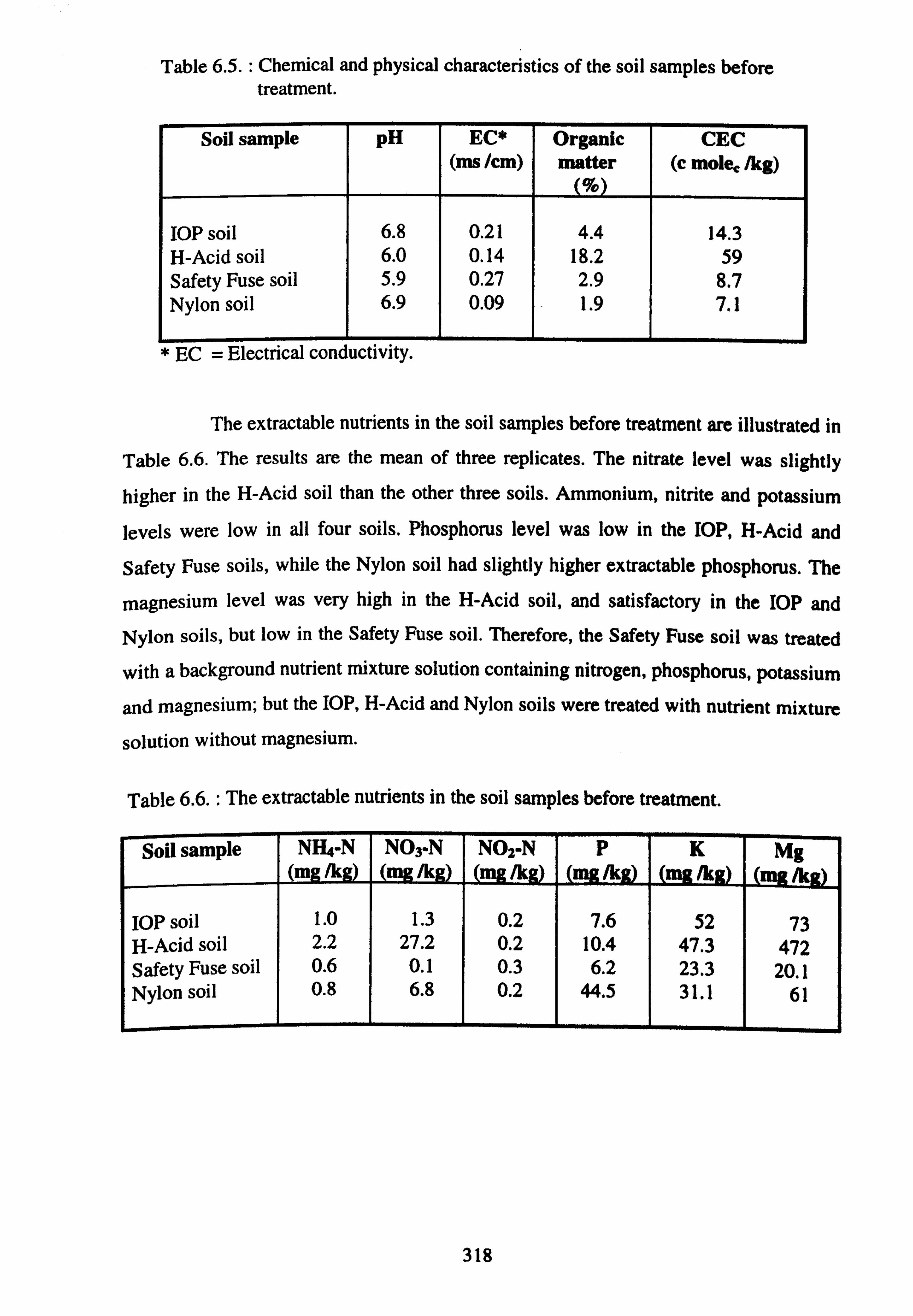
Table 6.5.: Chemical and physical characteristics of the soil samples before treatment.

Soil sample PH EC* Organic CEC (ms /cm) matter (c mole, /kg)

IOP soil 6.8 0.21 4.4 14.3 H-Acid soil 6.0 0.14 18.2 59 Safety Fuse soil 5.9 0.27 2.9 8.7 Nylon soil 6.9 0.09 1.9 7.1


The extractable nutrients in the soil samples before treatment are illustrated in

Table 6.6. The results are the mean of three replicates. The nitrate level was slightly

higher in the H-Acid soil than the other three soils. Ammonium, nitrite and potassium

levels were low in all four soils. Phosphorus level was low in the IOP, H-Acid and

Safety Fuse soils, while the Nylon soil had slightly higher extractable phosphorus. The

magnesium level was very high in the H-Acid soil, and satisfactory in the IOP and

Nylon soils, but low in the Safety Fuse soil. Therefore, the Safety Fuse soil was treated

with a background nutrient mixture solution containing nitrogen, phosphorus, potassium

and magnesium; but the IOP, H-Acid and Nylon soils were treated with nutrient mixture

solution without magnesium.

Table 6.6.: The extractable nutrients in the soil samples before treatment.

Soil sample NH4-N (mg/kg)

N03-N /k

N02-N Ak

P (mg/kg)

K /k

Mg Ak

IOP soil 1.0 1.3 0.2 7.6 52 73 H-Acid soil 2.2 27.2 0.2 10.4 47.3 472 Safety Fuse soil 0.6 0.1 0.3 6.2 23.3 20.1 Nylon soil 0.8 6.8 0.2 44.5 31.1 61

318


The chemical composition of the groundwater samples is summarised in

Table 6.7. The metal content of the groundwater samples is shown in Table 6.8. As can be seen, the pH was slightly high in all three wells. The well waters varied in the

nitrogen, electrical conductivity and composition of the dissolved salts. The heavy

metals were low in all well waters.

In terms of fertilising, the levels of nitrogen in the well waters determined the

irrigation volume. Well waters No. TW 8 and SW 11 had moderate nitrogen contents,

therefore, they were added at a high volume (100 ml per application three times a week

until the required volume 1.57 litre of well water No. TW 8 or 1.39 litre of well water

No. SW 11 was added). However, well water No. SW 15 had a very high nitrogen

content, therefore it was added at a low volume [7.7 ml of well water No. SW 15 diluted

in 100 ml was added in the beginning of the growth period in the case of the single

treatment and 1.7,1.5,1.5,1.5 and 1.5 ml of well water No. SW 15 diluted in 100 ml

was added at the start of each week in case of the split treatment]. Relative to the

nitrogen content in well waters No. SW 15 and TW 8, the electrical conductivity was

high in these wells, thus saline well waters were added but much diluted in the case of

well water No. SW 15.

Table 6.7. : Chemical composition of the groundwater samples.

Well No.

pH EC* (ms /cm)

NH4-N (mg /1)

N03-N (mg /1)

N02-N (mg /1)

Total N (mg /1)

TW 8 7.3 4.7 39.8 9.9 0.4 50.0 SW 11 8.0 0.7 51 5.0 <0.1 56 SW 15 7.5 62 4600 5580 0.1 10175

Well No.

Cl (mg /1)

K (rng /1)

Na m /1)

Ca (mg /1)

Mg (mg /1)

Fe m /1

TW 8 1170 53.8 126 520 297 95 SW 11 24.1 5.0 25.8 55 5.7 9.4 SW 15 343 350 1610 1380 1430 9.2


319

Table 6.8.: Metals content of the groundwater samples determined by the Inductively Coupled Plasma (ICP) Spectroscopy.

Well No.

Cu (mg /1)

Cd (mg /1

Cr (mg /1)

Zn (mg /1)

Ni (mg /1

Pb (mg /1

TW 8 <0.01 <0.01 <0.01 0.3 <0.01 <0.1 SW 11 <0.01 <0.01 <0.01 0.4 <0.01 <0.1 SW 15 <0.01 <0.01 <0.01 0.6 0.21 <0.1

Well No.

B (mg /1)

Ba (m /1)

Mn m /1

K m /1

TW 8 107 0.04 1.0 50.7 SW 11 0.82 0.30 0.3 5.9 SW 15 1.12 0.08 7.9 324

320

6.3.3. POT EXPERIMENT

The pot experiment was conducted to determine the influence of ammonium

and nitrate contaminated groundwater on the growth of the perennial ryegrass Lolium

eine L. ) and soil. In addition, the experiment was carried out to evaluate the

efficiency of the perennial ryegrass (Lolium perenne L. ) in the remediation of high

ammonium and nitrate contaminated groundwater under controlled conditions in the

greenhouse.

The fresh yield of the shoots is shown in Table 6.9. The results are the mean of

five replicates. The overall view of the pot experiment in the first period of treatment is

presented in Figure 6.1. The comparison of the grass treated with the well water

treatments and the control treatment in the first period of treatment is illustrated in

Figure 6.2.

321

Table 6.9. : The fresh yield of the shoots.

Soil and treatment Fresh yield of shoots Fresh yield of shoots [First period] [Second period]

( /pot) /pot)

IOP soil (Soil No. 1) :

Standard N, P, K control (single) 13.75 17.14 Well water No. TW 8 (split) 1.70 ----- Well water No. SW 11 (split) 11.84 16.26 Well water No. SW 15 (single) 13.02 16.95 Well water No. SW 15 (split) 12.09 17.73

H-Acid soil (Soil No. 9) :

Standard N, P, K control (single) 14.84 20.25 Well water No. TW 8 (split) 2.97 Well water No. SW 11 (split) 13.37 18.11 Well water No. SW 15 (single) 14.82 17.90 Well water No. SW 15 (split) 12,43 18.34

Safety Fuse soil (Soil No. 11) :

Standard N, P, K control (single) 13.72 16.30 Well water No. TW 8 (split) 1.35 ----- Well water No. SW 11 (split) 12.32 17.50 Well water No. SW 15 (single) 13.09 15.48 Well water No. SW 15 (slit) 11.30 15.76

Nylon soil (Soil No. 15) :

Standard N, P, K control (single) 14.34 18.73 Well water No. TW 8 (split) 1.76 Well water No. SW 11 (split) 11.75 17.51 Well water No. SW 15 (single) 13.64 17.84 Well water No. SW 15 (split) 11.64 16.47

t_T,... 1A - "W J

322

j

-. 7I, i, `

;. ý .

555 f `ý a

Figure 6.1.: The overall view of the pot experiment in the first period of h eaitnwent.

Tr

Figure 6.2.: The comparison of the grass treated with the wcll water treatments and the control treatment in the first period of treatment.

323

The grass growth was classified in the first period of treatment as shown in

Table 6.10.

Table 6.10.: The classification of the grass growth in the first period of treatment.

Treatment Grass

Stem Leaf Growth

Standard N, P, K control Tall. Tall, thick and Good. (single treatment). dark green.

Well water No. TW 8 Short. Short, thin and Poor. (split treatment). green-yellow.

Well water No. SW 11 Tall. Tall, thick and Good. (split treatment). dark green.

Well water No. SW 15 Tall. Tall, thick and Good. (single treatment). dark green.

Well water No. SW 15 Tall. Tall, thick and Good. (split treatment). dark green.

The grass treated with well waters No. SW 11 (split treatment), SW 15

(single treatment) and SW 15 (split treatment) was growing well indicating that it was

taking up sufficient nitrogen from the well water (see figure 6.2. ). The growth of grass

treated with well water No. TW 8 (split treatment) was very poor suggesting a toxicity

effect.

The dry yield of the shoots and roots is given in Table 6.11. The results are

the mean of five replicates. The dry yield of the shoots of the second period of treatment

was slightly higher than that of the first period of treatment in all four soils. This is

possibly due to the day length (sunshine hours) and the intensity of sunshine; but since

the first period of treatment was carried out in June and July, 1998 and the second

period of treatment was carried out in July and September, 1998 it is more likely due to

the residual effects of nitrogen of the previous treatments.

324

The residual effect could be due to nitrogen mobilisation from the roots and

stubble. Wilkins et al. (1997) assessed the varietal differences in rates of N03-N uptake

and remobilisation of nitrogen (N) during a cycle of severe defoliation and regrowth in

perennial ryegrass (Lolium perenne L. ) varieties Ba11778, Aberelan, Talbot and Gator.

They demonstrated that more N was remobilised from the roots than from the stubble

after defoliation. However, there were no significant differences among varieties in the

amount and rate of N remobilisation following defoliation.

Regarding the dry yield of the shoots of the first and second period; in all

four soils, the dry yield of grass treated with well water No. SW 15 (single treatment)

and the control treatment (single treatment) was more than that of grass treated with the

other treatments. This is attributed to the fact that the nitrogen fertiliser was added at the

start of the growth period, and consequently being used more efficiently to produce dry

matter yield.

The grass treated with well water No. TW 8 had the lowest dry yield in all four soils in the first period of treatment and it did not grow in the second period of

treatment. Among the well water treatments, well water No. SW 15 (single treatment)

was superior in producing dry yield in all four soils. In the five treatments, the dry yield

of grass grown in the H-Acid soil was slightly higher than that grown in the other three

soils.

In the case of the shoots of the first period, the Tukey LSD test (p = 0.05)

showed that in all four soils, the dry yield of grass treated with well water No. TW 8 was

significantly different from that of grass treated with the other well water treatments. In

all four soils, the dry yield of grass treated with well water No. SW 11 was not

significantly different (at 5% level) from that of grass treated with well water No. SW

15 (split treatment), while the dry yield of grass treated with well water No. SW 15

(single treatment) was significantly different from that of grass treated with well water No. SW 15 (split treatment). In the IOP, Safety Fuse and Nylon soils, the dry yield of

grass treated with the well water treatments was significantly different from that of grass

treated with the control treatment. In the H-Acid soil, the dry yield of grass treated with

well waters No.. TW 8, SW 11 and SW 15 (split treatment) was significantly different

from that of grass treated with the control treatment, while the dry yield of grass treated

325

with well water No. SW 15 (single treatment) was not significantly different from that

of grass treated with the control treatment.

In the case of the shoots of the second period; the Tukey LSD test (p = 0.05)

showed that in the IOP and Nylon soils, the dry yield of grass treated with well waters

No. SW 11 and SW 15 (split treatment) was significantly different (at 5% level) from

that of grass treated with the control treatment, while the dry yield of grass treated with

well water No. SW 15 (single treatment) was not significantly different from that of

grass treated with the control treatment. In the H-Acid soil, the dry yield of grass treated

with the well water treatments was significantly different from that of grass treated with

the control treatment. In the Safety Fuse soil, the dry yield of grass treated with the well

water treatments was not significantly different from that of grass treated with the

control treatment. The dry yield of grass treated with well water No. SW 15 (single

treatment) was not significantly different from that of grass treated with well water No.

SW 15 (split treatment) in the H-Acid and Safety Fuse soils, and was significantly

different from that of grass treated with well water No. SW 15 (split treatment) in the

IOP and Nylon soils.

The dry yield of the roots was higher than that of the shoots of the first or

second period of treatment.

Regarding the dry yield of the roots, the Tukey LSD test (p = 0.05) showed

that in the IOP, Safety Fuse and Nylon soils; the dry yield of grass treated with well

waters No. SW 11, SW 15 (single treatment) and SW 15 (split treatment) was not

significantly different (at 5% level) from that of grass treated with the control treatment,

while the dry yield of grass treated with well water No. TW 8 was significantly different

from that of grass treated with the control treatment and the other well water treatments.

In the H-Acid soil, the dry yield of grass treated with well waters No. TW 8, SW 11 and

SW 15 (split treatment) was significantly different from that of grass treated with the

control treatment; while the dry yield of grass treated with well water No. SW 15 (single

treatment) was not significantly different from that of grass treated with the control

treatment. The dry yield of grass treated with well water No. SW 15 (single treatment)

was not significantly different from that of grass treated with well water No. SW 15

(split treatment) in the IOP, Safety Fuse and Nylon soils, but was significantly different

326

from that of grass treated with well water No. SW 15 (split treatment) in the H-Acid

soil.

Table 6.11.: The dry yield of the shoots and roots.

Soil and treatment Dry yield of Dry yield of Dry yield of shoots shoots roots

[First period] [Second period] (g /pot)* ( /pot)* (g /pot)*


Standard N, P, K control (single) 3.43 a 4.42 a 13.36 a Well water No. TW 8 (split) 0.59 d ----- 3.47 b Well water No. SW 11 (split) 2.40 c 3.27 b 9.77 a Well water No. SW 15 (single) 2.98 b 4.29 a 10.48 a Well water No. SW 15 (split) 2.33 c 3.90 ab 9.50 a


Standard N, P, K control (single) 3.61 a 5.42 a 8.37 ab Well water No. TW 8 (split) 1.12 c ----- 3.28 c Well water No. SW 11 (split) 2.40 b 3.34 c 6.09 be Well water No. SW 15 (single) 3.18 a 4.41 b 7.56 ab Well water No. SW 15 (split) 2.47 b 4.15 b 10.19 a


Standard N, P, K control (single) 3.36 a 3.61 a 9.32 a Well water No. TW 8 (split) 0.50 d ----- 2.87 b Well water No. SW 11 (split) 2.22 c 3.29 a 9.75 a Well water No. SW 15 (single) 2.80 b 3.71 a 11.38 a Well water No. SW 15 (split) 2.13 c 3.52 a 12.14 a


Standard N, P, K control (single) 3.38 a 4.87 a 12.35 a Well water No. TW 8 (split) 0.64 d ----- 3.54 b Well water No. SW 11 (split) 2.13 c 3.51 b 10.33 a Well water No. SW 15 (single) 2.74 b 4.45 a 9.07 a Well water No. SW 15 (split) 2.16 c 3.87 b 13.61 a

_____ = No yield. * For each soil, mean values followed by same letter within a column are not

significantly different at 5% level using Tukey LSD test.

327

Well water No. TW 8 had a clear negative effect on the growth of grass as

the yield of this treatment was the lowest in all four soils in the first period and there

was no growth in the second period. Toxicity symptoms appeared on the grass of the

pots treated with this well water (see Figures 6.3. and 6.4. ). Toxicity symptoms appeared

on the grass 19 /6/ 1998 just 10 days after the start of the applications of well water

No. TW 8.

These toxicity symptoms were as follows :

- The grass had poor growth and was clearly dying.

- The leaves were short and had light green or green yellow colour (chlorosis) with

spotting of brown colour (dead leaf tissue) at the tips and the edges and toward the

centre between the veins.

There was also an iron precipitate (orange colour) on the soil surface.

These symptoms were toxicity symptoms not deficiency symptoms because

the grass for each soil treated with the control treatment was growing well indicating no

micro or macro nutrients deficiency. These toxicity symptoms were not related to

aluminium or manganese toxicity because the pH of well water No. TW 8 was not

acidic. These toxicity symptoms seemed to be related to boron because further analysis

of composition of well water No. TW 8 showed high level of boron (107 mg /1).

Alternatively, it may have been related to salinity effect as well water No. TW 8 had

high electrical conductivity (4.7 ms /cm).

Ayers and Westcot (1985) reported that boron toxicity symptoms normally

show first on older leaves as a yellowing, spotting, or drying of leaf tissue at the tips and

edges. As more and more boron accumulates with time, drying and chlorosis often

progress toward the centre between the veins (interveinal). In addition, on seriously

affected trees such as almonds and other tree crops which do not show typical leaf

symptoms, a gum or exudate on limbs or trunk is often noticeable.

These symptoms match the symptoms appeared on the grass treated with well

water No. TW 8.

328

Fleming (1980) reported that when the boron concentrations associated with different degrees of injury were measured, necrotic spots usually contained over 1500

mg /1 B while chlorotic tissue levels were mostly between 1000 and 1500 mg /1 B.

Richards (1954) pointed out that boron is very toxic to certain plant species,

however, the concentration that will injure these sensitive plants is often approximately

that required for normal growth of very tolerant plants. For instance, lemons show

definite and, at times, economically important injury when irrigated with water

containing 1.0 mg /I of boron, while alfalfa will make maximum growth with 1.0 to 2.0

Mg /I of boron.

Ayers and Westcot (1985) reported that boron is needed in relatively small

amounts, however, it becomes toxic if present in amounts appreciably greater than

needed. For some crops, if 0.2 mg /I boron in water is essential, 1.0 to 2.0 mg /1 may be

toxic. As the boron concentrations in leaf blades exceed 250 - 300 mg /kg (dry weight),

most crop toxicity symptoms result, however, not all sensitive crops accumulate boron

in leaf blades.

The toxicity effects were severe in the IOP, Safety Fuse and Nylon soils but

were less so in the H-Acid soil. On 20 /7/ 1998,42 days after the start of the

applications of well water No. TW 8, the grass of the H-Acid soil had about 40 % live

buds and about 60 % dead grass but the grass of the IOP, Safety Fuse and Nylon soils had about 10 % live buds and about 90 % dead grass. The H-Acid soil was resisting the

toxicity of boron possibly because of its high clay content and high organic matter

content.

Fleming (1980) showed that the great availability of boron in surface soils

compared with subsurface soils, is undoubtedly related to relative organic matter levels

and in humid regions, where any soluble salts are readily leached out, available boron is

largely held in the organic fraction. Light-textured soils contain less available boron

than heavy textured soils and boron deficiency is more common in them because of less

binding and therefore greater leaching. In alkaline soils where free calcium ions are

present, boron availability is much less; therefore, under these conditions more boron is

required to prevent deficiency while on the other hand plants can tolerate amounts of

boron that would normally prove toxic.

329

s\

;ý

\:

ý- ý ý,

ý.... ýý ýý : ý. ý -ý

,=r

330

Figure b. 3.: The comparison of the grass treated with well water No. 'I'W 8 and the control treatment in the first period of treatment.

f'Iblllý o. ý. l ýuaý .ýEýý! (illy lw\i, i\ ýýIllj)lOlllý III ýýI: 111 llcltcd \\ Jill \\ CH

water No. TW 8 in the first period of treatment.

The nitrogen (%) in the shoots and roots is summarised in Table 6.12. The

results are the mean of five replicates. As can be seen, the nitrogen (%) of the shoots

was slightly higher than that of roots.

Regarding the shoots of the first period, the results for well water No. TW 8

were influenced by the boron toxicity, and the application of this treatment was stopped

and the grass died. Therefore, the nitrogen results were not meaningful. Well water No.

SW 15 (split treatment) gave higher nitrogen (%) but lower dry yield than well water

No. SW 15 (single treatment) and this is attributed to that well water No. SW 15 (split

treatment) had nitrogen late at the end of the first period but was unable to make use of

it.

The Tukey LSD test (p = 0.05) showed that in all four soils, the nitrogen (%)

in grass treated with well waters No. TW 8, SW 11 and SW 15 (split treatment) was

significantly different (at 5% level) from that in grass treated with the control treatment.

The nitrogen (%) in grass treated with well water No. SW 15 (single treatment) was not

significantly different from that in grass treated with the control treatment in the IOP,

Safety Fuse and Nylon soils; and was significantly different from that in grass treated

with the control treatment in the H-Acid soil. In all four soils, the nitrogen (%) in grass

treated with well water No. SW 15 (single treatment) was significantly different from

that in grass treated with well water No. SW 15 (split treatment).

Regarding the shoots of the second period, the shoots of grass treated with

well water No. SW 11 had higher nitrogen (%) than that treated with the other

treatments in all four soils and this could be because the grass treated with well water

No. SW II had dry yield slightly lower than that treated with the other treatments. The Tukey LSD test (p = 0.05) showed that the nitrogen (%) in grass treated

with well water No. SW 11 was significantly different (at 5% level) from that in grass

treated with the control treatment in the IOP, H-Acid and Nylon soils; but not

significantly different from that in grass treated with the control treatment in the Safety

Fuse soil. The nitrogen (%) in grass treated with well water No. SW 15 (single

treatment) was significantly different from that in grass treated with the control

treatment in the IOP and Safety Fuse soils; and not significantly different from that in

grass treated with the control treatment in the H-Acid and Nylon soils. The nitrogen (%)

331

in grass treated with well water No. SW 15 (split treatment) was not significantly

different from that in grass treated with the control treatment in the H-Acid soil; while it

was significantly different from that in grass treated with the control treatment in the

IOP, Safety Fuse and Nylon soils. The nitrogen (%) in grass treated with well water No.

SW 15 (single treatment) was significantly different from that in grass treated with well

water No. SW 15 (split treatment) in the IOP, Safety Fuse and Nylon soils; and not

significantly different from that in grass treated with well water No. SW 15 (split

treatment) in the H-Acid soil.

Regarding the roots, the nitrogen (%) in the roots was slightly lower than that

of the shoots. In the five treatments, the nitrogen (%) in the roots of grass grown in the

H-Acid soil was slightly higher than that of grass grown in the other three soils.

The Tukey LSD test (p = 0.05) showed that the nitrogen (%) in grass treated

with the well water treatments was significantly different (at 5% level) from that in

grass treated with the control treatment in the IOP soil, and not significantly different

from that in grass treated with the control treatment in the Safety Fuse soil. In the H-

Acid soil, the nitrogen (%) in grass treated with well waters No. TW 8, SW 15 (single

treatment) and SW 15 (split treatment) was significantly different from that in grass

treated with the control treatment, while the nitrogen (%) in grass treated with well

water No. SW 11 was not significantly different from that in grass treated with the

control treatment. In the Nylon soil, the nitrogen (%) in grass treated with well waters

No. TW 8 and SW 15 (single treatment) was not significantly different from that in

grass treated with the control treatment, but the nitrogen (%) in grass treated with well

waters No. SW 11 and SW 15 (split treatment) was significantly different from that in

grass treated with the control treatment. The nitrogen (%) in grass treated with well

water No. SW 15 (single treatment) was not significantly different from that in grass

treated with well water No. SW 15 (split treatment) in the IOP, H-Acid and Safety Fuse

soils, however, it was significantly different from that in grass treated with well water

No. SW 15 (split treatment) in the Nylon soil.

332

Table 6.12. : Nitrogen (%) in the shoots and roots.

Soil and treatment N (%) of shoots N (%) of shoots N (%) of [First period] * [Second period] * roots*


Standard N, P, K control (single) 1.07 c 1.00 be 0.53 b Well water No. TW 8 (split) 2.25 a ----- 0.62 ab Well water No. SW 11 (split) 1.43 b 1.35 a 0.74 a Well water No. SW 15 (single) 1.05 c 0.88 c 0.65 ab Well water No. SW 15 (split) 1.57 b 1.10 b 0.65 ab


Standard N, P, K control (single) 1.21 c 0.99 b 0.90 a Well water No. TW 8 (split) 2.52 a ----- 0.84 ab Well water No. SW 11 (split) 1.47 b 1.31 a 0.90 a Well water No. SW 15 (single) 1.04 d 0.96 b 0.78 b Well water No. SW 15 (split) 1.40 b 1.09 b 0.80 b


Standard N, P, K control (single) 0.94 d 1.21 a 0.73 a Well water No. TW 8 (split) 2.23 a ----- 0.63 a Well water No. SW 11 (split) 1.37 c 1.30 a 0.61 a Well water No. SW 15 (single) 1.03 d 0.88 b 0.56 a Well water No. SW 15 (split) 1.54 b 1.13 ab 0.54 a


Standard N, P, K control (single) 1.14 c 0.98 c 0.56 ab Well water No. TW 8 (split) 2.40 a ----- 0.65 ab Well water No. SW 11 (split) 1.59 b 1.28 a 0.72 a Well water No. SW 15 (single) 1.28 c 0.93 c 0: 64 ab Well water No. SW 15 (split) 1.63 b 1.12 b 0.53 b

----- = 1V o ylela.


333

The nitrogen yield in the shoots and roots and the apparent nitrogen (%)

recovered in the shoots are presented in Table 6.13. The results are the mean of five

replicates. It was observed that the nitrogen yield in the shoots of the second period was

higher than that of the first period. The nitrogen yield in the roots was higher than that in

the shoots of the first or second period of treatment.

In the case of the shoots of the first and second period, the nitrogen yield in

grass treated with the well water treatments was lower than that in grass treated with the

control treatment in all soils except the Safety Fuse soil. The nitrogen yield in grass

treated with well water No. SW 15 (split treatment) was higher than that in grass treated

with well water No. SW 15 (single treatment) in all four soils. The nitrogen yield in

grass grown in the H-Acid soil was higher than that in grass grown in the other three

soils. Among the four soils, the nitrogen yield in grass grown in the Safety Fuse soil was

the lowest in the five treatments.

In all soils except the IOP soil, well water No. SW 15 (split treatment)

produced higher nitrogen yield in the roots than well water No. SW 15 (single

treatment). The nitrogen yield in the roots of grass grown in the H-Acid soil was higher

than that of grass grown in the other three soils.

The total nitrogen yield in the shoots was calculated by adding together the

nitrogen yield of shoots of both the first and second period of treatment. The grass

treated with well water No. SW 15 (split treatment) and the control treatment was more

efficient in nitrogen uptake than that treated with well water No. SW 15 (single

treatment) in all four soils. The total nitrogen yield in the shoots of grass grown in the

H-Acid soil was higher than that of grass grown in the other three soils, however, the

total nitrogen yield in the shoots of grass grown in the Safety Fuse soil was lower than

that of grass grown in the other three soils.

The Tukey LSD test (p = 0.05) showed that the total nitrogen yield in the

shoots of grass treated with the well water treatments was significantly different (at 5%

level) from that of grass treated with the control treatment in the H-Acid and Nylon

soils. In the IOP and Safety Fuse soils, the total nitrogen yield in the shoots of grass

treated with well waters No. SW 11 and SW 15 (split treatment) was not significantly

334

different from that of grass treated with the control treatment, while the total nitrogen

yield in the shoots of grass treated with well water No. SW 15 (single treatment) was

significantly different from that of grass treated with the control treatment. The total

nitrogen yield in the shoots of grass treated with well water No. SW 15 (single

treatment) was significantly different from that of grass treated with well water No. SW

15 (split treatment) in the IOP and Safety Fuse soils, but not significantly different from

that of grass treated with well water No. SW 15 (split treatment) in the H-Acid and Nylon soils.

The apparent nitrogen (%) recovered in the shoots was calculated from the

total nitrogen yield of the shoots. The apparent nitrogen (%) recovered in the shoots of

grass treated with well water No. TW 8 was not calculated because the grass died. The

grass treated with well water No. SW 15 (single treatment) had the lowest efficiency in

nitrogen uptake in all four soils. The apparent nitrogen (%) recovered in the shoots of

grass grown in the H-Acid soil was higher than that of grass grown in the other three

soils, however, the apparent nitrogen (%) recovered in the shoots of grass grown in the Safety Fuse soil was lower than that of grass grown in the other three soils.

335

Table 6.13.: The nitrogen yield in the shoots and roots and the apparent nitrogen (%) recovered in the shoots.

Soil and treatment N yield N yield N yield Total N Apparent of shoots of shoots of roots yield of nitrogen

[First [Second (mg/pot) shoots* (%) Period] Period] (mg/pot) recovered m /pot) m /pot) in shoots


Standard N, P, K control(single) 36.84 44.05 68.74 80.89 a 51.5 Well water No. TW 8 (split) 13.22 ----- 21.18 13.22 ---- Well water No. SW 11 (split) 34.28 43.85 68.80 78.14 a 49.8 Well water No. SW 15 (single) 31.32 37.26 66.62 68.57 b 43.7 Well water No. SW 15 (split) 36.36 42.59 60.76 78.94 a 50.3


Standard N, P, K control(single) 43.59 53.60 75.10 97.19 a 61.9 Well water No. TW 8 (split) 28.25 ----- 27.25 28.25 ---- Well water No. SW 11 (split) 35.27 43.61 54.12 78.88 b 50.2 Well water No. SW 15 (single) 32.85 41.57 58.81 74.42 b 47.4 Well water No. SW 15 (split) 34.58 45.08 81.69 79.66 b 50.7


Standard N, P, K control(single) 31.59 42.00 64.58 73.59 a 46.9 Well water No. TW 8 (split) 11.09 ----- 18.18 11.09 ---- Well water No. SW 11 (split) 30.45 42.73 56.90 73.18 a 46.6 Well water No. SW 15 (single) 28.75 32.49 59.64 61.24 b 39.0 Well water No. SW 15 (split) 32.69 39.55 64.07 72.24 a 46.0


Standard N, P, K control(single) 38.70 47.49 67.06 86.20 a 54.9 Well water No. TW 8 (split) 15.15 ----- 23.12 15.15 ----- Well water No. SW 11 (split) 33.90 45.08 74.09 78.98 b 50.3 Well water No. SW 15 (single) 35.07 41.32 57.53 76.39 b 48.7 Well water No. SW 15 (split) 35.12 43.29 67.43 78.41 b 49.9

----- = No yield. * For each soil, mean values followed by same letter within a column are not

significantly different at 5% level using Tukey LSD test. Treatment with well water No. TW 8 was not included in the statistical analysis.

336

The residual nitrogen and nitrogen (%) remaining in the soil after treatment are

shown in Table 6.14. The results are the mean of five replicates. As can be seen,

ammonium and nitrate were the dominant ions remaining in the soil at the end of the pot

experiment, but ammonium level was higher than the nitrate and nitrite levels in all four

soils.

The grass treated with well water No. TW 8 resulted in higher residual

nitrogen in all four soils than that treated with the other four treatments. The grass

treated with well water No. SW 15 (single treatment ) resulted in slightly higher residual

nitrogen in all four soils than that treated with well water No. SW 15 (split treatment).

The grass treated with the control treatment gave the lowest residual nitrogen in all soils

except the Safety Fuse soil. The residual nitrogen in the H-Acid soil was higher than in

the other three soils.

The Tukey LSD test (p = 0.05) showed that the residual nitrogen in the IOP,

H-Acid and Safety Fuse soils with the well water treatments was not significantly

different (at 5% level) from that with the control treatment. The residual nitrogen in the

Nylon soil with well waters No. SW 11 and SW 15 (single treatment) was significantly

different from that with the control treatment, but the residual nitrogen with well water

No. SW 15 (split treatment) was not significantly different from that with the control

treatment. The residual nitrogen in the IOP, H-Acid and Safety Fuse soils with well

water No. SW 15 (single treatment) was not significantly different from that with well

water No. SW 15 (split treatment), while the residual nitrogen in the Nylon soil with

well water No. SW 15 (single treatment) was significantly different from that with well

water No. SW 15 (split treatment).

The nitrogen (%) remaining in soil was calculated from the residual nitrogen

in soil. The nitrogen (%) remaining in the soil with well water No. TW 8 was not

calculated because the grass died. There was very little nitrogen remaining in all four

soils as inorganic nitrogen only 0.2 - 2.46 % of nitrogen applied.

337

Table 6.14.: The residual nitrogen and nitrogen (%) remaining in the soil after treatment.

Soil and treatment NH4-N N03-N NO2-N Residual N (mg g) (mg 1k8) (mg/kg) N (%) in soil in soil in soil (mg /pot) remaining

in soil* in soil


Standard N, P, K control (single) 0.64 0.13 0.21 0.59 a 0.38 Well water No. TW 8 (split) 3.20 2.44 0.17 3.49 ----- Well water No. SW 11 (split) 1.58 1.41 0.26 1.95 a 1.24 Well water No. SW 15 (single) 1.56 1.13 0.31 1.80 a 1.15 Well water No. SW 15 (split) 1.04 0.91 0.26 1.33 a 0.85






Standard N, P, K control (single) 0.80 0.00 0.21 0.50 b 0.32 Well water No. TW 8 (split) 5.45 2.24 0.04 4.63 ----- Well water No. SW 11 (split) 1.29 1.64 0.09 1.81 a 1.15 Well water No. SW 15 (single) 1.22 0.46 0.21 1.14 ab 0.72 Well water No. SW 15 (split) 0.71 0.50 0.08 0.75 b 0.48

* For each soil, mean values followed by same letter within a column are not significantly different at 5% level using Tukey LSD test. Treatment with well water No. TW 8 was not included in the statistical analysis.

338

6.4. CONCLUSION FOR THE BIOREMEDIATION OF THE

AMMONIUM AND NITRATE CONTAMINATED WATER

USING NATURAL SOIL AND VEGETATION

The groundwater quality surveys at the Ardeer site revealed that the majority

of the wells had pH in the range from 6.1 to 8.3 but some wells were acidic (pH below

4.3). Ammonium contamination was quite localised at the site. The nitrate

contamination was also very closely localised but ammonium and nitrate were not

necessarily found together (see Map 6.1. ). Chloride, sodium, potassium, calcium,

magnesium and iron contamination was widespread at the site. High electrical

conductivity was widespread at the site. Well No. SW 15 was the most badly

contaminated well on the site.

The soil survey at the Ardeer site demonstrated that the level of nutrients (N,

P. K) was low in all four investigated areas (IOP, H-Acid, Safety Fuse and Nylon areas).

The levels of toxic metals were low in the soils. Overall, the variations in vegetation

cover appear to be due to differences in macronutrient availability rather than any

toxicity.

From the preliminary experiment of nitrification, it was concluded that the

Safety Fuse and Nylon soils had extremely low nitrification rates and were not suitable

for further studies. The Intermediate Oxidation Plant (IOP) and H-Acid soils were

suitable for subsequent work together with two garden natural soils (Darvel and

Dreghorn) which were used for comparison.

The nitrification experiment showed that well water No. SW 11 showed no

inhibition in all four soils. Well water No. SW 15 showed significant inhibition in the

IOP, Dreghorn and H-Acid soils but not in the Darvel soil. Well water No. TW 8

significantly inhibited all the soils to the extent that nitrification was barely measurable

in the Dreghorn, IOP and H-Acid soils.

339

339a

Map 6.1.: Groundwater wells with elevated levels of ammonium and nitrate at the Ardeer site.

The results of the pot experiment showed that well water No. TW 8 had a

clear negative effect on the growth of grass as the yield of this treatment was the lowest

in all four soils in the first period and there was no growth in the second period.

Toxicity symptoms appeared on the grass of the pots treated with this well water.

The grass treated with well water No. SW 15 (split treatment) and the control

treatment (single treatment) was more efficient in nitrogen uptake than that treated with

well water No. SW 15 (single treatment) in all four soils. There was very little nitrogen

remaining in all four soils as inorganic nitrogen only 0.2 - 2.46 % of nitrogen applied.

These results of the pot experiment suggest the possibility of applying the bioremediation treatment of the ammonium and nitrate contaminated water in the field

at the Ardeer site. A field study should be undertaken to evaluate the efficiency of this

bioremediation treatment. This field study would require a suitable uniform area to

layout the plots, preferably close to the source of water to be used. In addition, it is

necessary to carry out a hydrological survey to determine the following aspects :

1- The size of groundwater reservoir.

2- The rate of removal of the water.

3- The time scale of the water application.

The IOP area is unsuitable because of the varying chemical properties in the

topsoils and subsoils. The imported topsoil had varying depth (ranged from 6.0 to 15

cm) and overlying building rubble, concrete , brick, ash, sand and stony rubble. In

addition, the bottoming for the IOP building was probably slag from the adjacent former

iron works. There are slightly higher levels of barium in the subsoil on parts of the area

than is typical of the site. Relative to the ICRCL Guidance Note 59 /83 (1987), the

subsoil of the sample site No. 2 exceeded the threshold value for copper and nickel. The

subsoil of the sample site No. 1 was on the borderline of the threshold value for zinc

(see Map 4.4. ).

The imported topsoil on the H-Acid area is overlying concrete, building

rubble and sand. The depth varied from 11.0 to 22.0 cm. Relative to the ICRCL

340

Guidance Note 59 /83 (1987), the topsoil and subsoil of the sample site No. 9 exceeded

the threshold value for nickel. Nevertheless, the existing grass cover was uniform and

good, therefore, this area may be suitable to be used (see Map 4.5. ).

The imported topsoil on the Safety Fuse area is more uniform in depth and

generally overlying a sandy subsoil, however, the pH is rather variable and on part of the

area the topsoil overlies asphalt rubble in the case of site No. 12 ( see Map 4.6. ).

The Nylon area is sandy with some development of a natural topsoil. There is

concrete and building rubble over a wide area but the rest of the area could be

cultivated. Relative to the ICRCL Guidance Note 59 /83 (1987), the topsoil of the

sample site No. 17 exceeded the threshold value for copper and was on the borderline of

the threshold value for zinc. Therefore, site No. 17 should be excluded from the field

study due to the potential toxicity of copper and zinc to grass (see Map 4.7. ).

All of the site has some problems of uniformity but carefully selected areas of

H-Acid, Safety Fuse and Nylon could be identified to layout a field trial. A background

of phosphorus and potassium (magnesium) fertiliser would be required and some areas

might require liming. A careful preliminary uniformity test would be necessary.

The groundwater sources with elevated levels of ammonium-N available to be

used in this field study are :

Well water No. SW 15 has a very high level of ammonium (8090 mg /1) and

well water No. SW 16 has high level of ammonium (117 mg /1). Well waters No. SW

11, SW 14, SW 107, TW 8, TW 104 - TW 106, TW 112 and TW 114 have moderate

levels of ammonium (in the range of 17.0 to 58.0 mg /1) [see Map 6.1. ].

The groundwater sources with elevated levels of nitrate-N available to be used

in this field study are :

Well waters No. SW 14, SW 15 and SW 18 have very high levels of nitrate (in

the range of 2701 to 10860 mg /1). Well waters No. SW 6, SW 16 and SW 23 have high

levels of nitrate (in the range of 121 to 840 mg /1). Well waters No. SW 2, SW 3, SW

11, TW 2, BH 7 and BH 9 have moderate levels of nitrate (in the range of 14.0 to 45.5

mg /1) [see Map 6.1. ].

341

A suitable groundwater source for a field study in the Safety Fuse and H-

Acid areas are well waters No. SW 14, SW 15 and SW 16. These well waters can be

added at a low volume as a split treatment which was more efficient in nitrogen uptake

than the single treatment.

A suitable groundwater source for a field study in the Nylon area is well

water No. SW 11. This well water would have to be added at a high volume as a split

treatment.

The irrigation of ryegrass with highly contaminated groundwater could result

in problems such as salinity, high or low pH and toxicity. Salinity has an effect on the

physiology of plant as it decreases the growth as a result of insufficient water. Well

waters No. SW 14, SW 15 and SW 16 have very high electrical conductivity but since

they will be added as diluted water they should not cause a salinity problem. Well

waters No. SW 11 and SW 107 had low electrical conductivity and so should not cause

a salinity problem.

Well waters No. SW 15 and SW 11 have low levels of boron (1.12 and 0.82

mg /1, respectively) and can be added safely without causing potential boron toxicity to

grass. The cleaning of well water No. TW 8 from its high level of boron by a chemical

method makes the bioremediation treatment too costly. In addition, the iron level in well

water No. TW 8 is high (95 mg /1), therefore, well water No. TW 8 should be avoided

for this field study.

The climatic conditions such as rainfall, potential evapotranspiration and

temperature should be taken into consideration when carrying out the bioremediation


growth of grass. The water requirements for grass varies from the winter months to the

summer months due to these climatic conditions.

The average monthly rainfall, potential transpiration and water requirements

for grass at the Ardeer site are presented in Table 6.15. As can be seen, on average, there

are two months (May and June) when irrigation could be applied without causing

leaching. Overall, 3 cm of irrigation water can be applied in these two months.

342

Table 6.15. : The average monthly rainfall, potential transpiration and water requirements for grass at the Ardeer site.

Month Rainfall (mm)*

Potential Transpiration (mm)**

Water requirements (mm)

January 91.01 6.35 ----- February 55.49 13.97 ----- March 58.82 33.02 ----- April 52.16 57.15 4.99 May 56.60 88.90 32.30 June 64.37 95.25 30.88 July 88.79 86.36 ----- August 101.00 69.85 ----- September 110.99 46.99 October 107.66 27.94 ----- November 109.88 10.16 ----- December 103.22 7.62 -----

*Source:

-A NON (1989).

-A NON (1977). ** Source :

-A NON (1967).

There is only one option to apply well waters with moderate levels of nitrogen

as follows :

Well water No. SW 11 is used as an example for well waters with moderate levels of nitrogen. Well water No. SW 11 had 83.6 mg /1 total nitrogen would have to be

applied at a high volume (300 m3) to provide 25.08 kg N /ha. This required volume (300

m) from well water No. SW 11 was calculated from the following equation :

Required volume for 1 hectare = 100 mx 100 mx0.03 m= 300 m3

Where :

1 hectare = 100 mx 100 m.

3 cm = 0.03 m (see Table 6.15. ).

The total nitrogen to be provided from well water No. SW 11 was calculated from the following equation:

343

Required volume for 1 hectare x Total nitrogen (mg /1) Total nitrogen (kg /ha) = -------------------------------------------------------- ----------------

1000

Where :

mg /1 =g /m3

There are several options to apply well waters with very high levels of

nitrogen as follows :

Well water No. SW 15 is used as an example for well waters with very high

levels of nitrogen.

First option :

The first option of applying well water No. SW 15 is to apply it at a low

volume. Well water No. SW 15 had 16190 mg /1 total nitrogen can be applied at a low

volume (6.18 m3) to provide 100 kg N /ha. This required volume (6.18 m3) from well

water No. SW 15 was calculated from the above equation used for calculating the total

nitrogen (kg /ha).

The advantage of applying well water No. SW 15 at low volume (6.18 m3) is

that this application can be applied at wet time in the year, however, the disadvantage is

that this application is too small to apply.

Second option :

The second option for applying well water No. SW 15 is to blend well water

from more than one well using well water No. SW 15, e. g., blending well water No. SW

11 with well water No. SW 15 to achieve a realistic irrigation rate at a suitable nitrogen

level.

344

Third option :

The third option of applying well water No. SW 15 might be to overirrigate in

expectation that the ammonium would be retained in the soil. This is more likely to

work with the H-Acid area (59.0 c mole,, /kg CEC) but not with the other three areas;

IOP, Safety Fuse and Nylon areas (CEC ranged from 7.1 to 14.3 c moles /kg). The

subsoil of the H-Acid area is sandy and permeable, therefore, waterlogging is not

expected.

345

GENERAL CONCLUSIONS

The current study was accomplished to investigate groundwater contamination

and bioremediation treatment for cleaning up groundwater contaminated with

ammonium and nitrate using natural soil and vegetation [perennial ryegrass (Lolium

ep renne L. )] at an contaminated industrial site, the Ardeer site. The study was carried

out using well waters from the suspected areas and soil samples from the selected areas

at the site.

The developed methods for measuring ammonium in soil and water,

measuring low levels of ammonium in groundwater (< 0.1 mg /1) and decolorising the

highly coloured groundwater samples were used to help the experimental work of the

study. The investigation of groundwater quality at the Ardeer site helped to identify the

sources of nitrogen contamination, to locate the distribution of ammonium-N, nitrate-N

and other contaminants, and to evaluate the groundwater quality parameters. The soil

survey at the Ardeer site helped to choose soil samples suitable for nitrification incubation experiment and pot experiment. The nitrification experiment helped to assess the effects of groundwater composition on the nitrification rate in soil and to determine

the ability of soils to nitrify ammonium and thus promote leaching as nitrate. The pot

experiment was undertaken to evaluate the efficiency of the perennial ryegrass (Lolium

ep renne L. ) in the remediation of high ammonium and nitrate groundwater. The results

of the pot experiment were successful.

The overall conclusion of this study is, therefore, the bioremediation

treatment of the ammonium and nitrate contaminated water can be applied in the field

over a period of years. A field study should be undertaken to evaluate the efficiency of this bioremediation treatment. This field study would require a suitable uniform area to lay out the plots, preferably close to the source of water to be used. In addition, it is

necessary to carry out a hydrological survey to determine the following aspects :

I- The size of groundwater reservoir.

2- The rate of removal of the water. 3- The time scale of the water application.

346

The climatic conditions such as rainfall, potential evapotranspiration and temperature should be taken into consideration when carrying out the bioremediation


growth of grass. There are three options to apply the contaminated groundwater as follows :

1- To apply the contaminated groundwater at low or high volume depending on its level

of nitrogen. 2- To blend well water with high level of nitrogen with well water with low level of

nitrogen to achieve a realistic irrigation rate at a suitable nitrogen level.

3- To overirrigate in expectation that ammonium would be retained in the soil.

The ryegrass used in this bioremediation treatment can be disposed of by the incineration and landfilling the ash or landfilling the grass.

347

REFERENCES

Abdel Hamid, M. W., and Hamdi, H. (1974). A suitability index of drainage waters for

irrigation purposes. Egypt J. Soil Sci., Vol. 14, No. 1, pp. 101 - 113.

Abu Zeid , M., and Biswas, A. K. (1990). Impacts of agriculture on water quality. Water

International, Vol. 15, No. 3, pp. 160 - 167.

Adamsen, F. J. (1989). Irrigation method and water quality effect on peanut yield and

grade. Agronomy Journal, Vol. 81, pp. 589 - 593.

ADAS (1981). Particle size distribution in soil. The analysis of agricultural materials.

Reference Book 427. Second edition, pp. 151 - 155. Ministry of Agriculture,

Fisheries and Food. HMSO, London.

Addiscott, T. M. (1983). Kinetics and temperature relationships of mineralization and

nitrification in Rothamsted soils with differing histories.. Journal of Soil

Science, Vol. 34, pp. 343 - 353.

Alawi, B. J., Stroehlein, J. L., Hanlon, E. A. Jr., and Turner, F. Jr. (1980). Quality of

irrigation water and effects of sulphuric acid and gypsum on soil properties and

sudangrass yields. Soil Science, Vol. 129, No. 5, pp. 315 - 319.

Alexander, M. (1977). Introduction to soil microbiology. Edited by Martin Alexander,

1977, second edition.

Alexander, M. (1994). Biodegradation and bioremediation. Edited by Martin Alexander,

1994.

Altman, S. J., and Parizek, R. R. (1995). Dilution of nonpoint-source nitrate in

groundwater. Journal of Environmental Quality, Vol. 24, pp. 707 - 718.

Amin, M. (1995). Studies on the measurement and behaviour of nitrogen in soil. Ph. D.

Thesis. University of Glasgow.

348

A NON (1967). Potential transpiration. Ministry of Agriculture, Fisheries and Food.

Technical Bulletin No. 16, pp. 19 - 51. HMSO.

A NON (1977). Map of average annual rainfall (1941 - 1970) of North Britain.

Published by the Meteorological Office in 1977.

A NON (1982). Chloride in water, sewage and effluents, 1981. Methods for

examination of water and associated materials. HMSO.

A NON (1989). The climate of Scotland : Some facts and figures. The Meteorological

Office, pp. 1- 22. HMSO.

Aoki, T., Uemura, S., and Munemori, M. (1986). Continuous flow method for

simultaneous determination of nitrate and ammonia in water. Environ. Sci.

Technol., Vol. 20, No. 5, pp. 515 - 517.

Araujo, A. N., Etxebarria, M. B., Lima, J. L. F. C., Montenegro, M. C. B. S. M., and Olmos, R. P. (1995). Flow injection analysis of high chloride levels in

electroplating baths using on-line dialysis and potentiometric detection.

Fresenius' Journal of Analytical Chemistry, Vol. 351, No. 7, pp. 614 - 617.

Archer, J. (1988). Crop nutrition and fertiliser use. Edited by John Archer, second

edition, 1988.

Ayers, R. S., and Westcot, D. W. (1985). Water quality for agriculture. FAO, Rome,

Irrigation and drainage paper No. 29 Rev. 1.

Azov, Y., and Tregubova, T. (1995). Nitrification processes in stabilisation reservoirs.

Water Science and Technology, Vol. 31, No. 12, pp. 313 - 319.

Bae, J. -H, Carbohydrate, K. -M., Park, S. -Y., Maeng, S. -M., and Song, K. -B. (1995).

Effects of retention time and ammonia on the treatment of leachate. J. Korea

Society of Water Quality, Vol. 11, pp. 323 - 332.

349

Bae, J. -H, Kim, S. -K., and Chang, H. -S. (1997). Treatment of landfill leachates : Ammonia removal via nitrification and denitrification and further cod reduction

via Fenton's treatment followed by activated sludge. Water Science and Technology, Vol. 36, No. 12, pp. 341 - 348.

Baker, A. J. M., and Walker, P. L. (1990). In Heavy Metal Tolerance in Plants : Evolutionary Aspects. Shaw, A. J. Ed. CRC Press. Boca Raton. FL 1990. pp. 155 - 177.

BDH Laboratory Supplies Catalogue (1997). Chemical and Reagents. BDH - Merck. Page 2- 411 - Polyacrylamide and page 2- 127 - Cetylpyridinium.

Becker, M., Martienssen, M., Fuhrmann, B., and Spohn, U. (1997). Analysing nitrogen

and sulphide elimination from leachate by colorimetric continuous flow titration. Acta Biotechnol., Vol. 17, No. 1, pp. 39 - 50.

Berg, B. R., and Abdullah, M. I. (1977). An automatic method for the determination of ammonia in sea water. Water Research, Vol. 11, pp. 637 - 638.

Best, E. K. (1976). An automated method for determining nitrate nitrogen in soil

extracts. Queensland Journal of Agriculture and Animal Sciences, Vol. 33, pp. 161-166.

Blaise, D., Amberger, A., and von Tucher, S. (1997). Influence of iron pyrites and dicyandiamide on nitrification and ammonia volatilisation from urea applied to loess brown earths (Luvisols). Biol. Fertil. Soils, Vol. 24, pp. 179 - 182.

Blevins, D. W., Wilkison, D. H., Kelly, B. P., and Silva, S. R. (1996). Movement of

nitrate fertiliser to glacial till and runoff from a claypan soil. Journal of Environmental Quality, Vol. 25, pp. 584 - 593.

Bohm, B. (1994). A test method to determine inhibition of nitrification by industrial

wastewaters. Water Science and Technology, Vol. 30, No. 6, pp. 169 - 172.

350

Bremner, J. M., and Mulvaney, C. S. (1982). Total nitrogen. In : Methods of Soil

Analysis (edited by A. L. Page, A. L., Miller, R. H., and Keeny, D. R. ). pp. 1119

- 1123. American Society of Agronomy and Soil Science Society of America, Madison, Wisconsin.

Brown, M. W. (1973). A highly sensitive automated technique for the determination of ammonium nitrogen. J. Sci. Food Agric., Vol. 24, pp. 1119 - 1123.

Burton, D. L., Gower, D. A., Rutherford, P. M., and Mcgill, W. B. (1989). Amino acid interference with ammonium determination in soil extracts using the automated indophenol method. Communications in Soil Science and Plant Analysis, Vol.

20, No. 5&6, pp. 555 - 565.

Burton, A. J., Hart, J. B., and Urie, D. H. (1990). Nitrification in sludge-amended Michigan forest soils. Journal of Environmental Quality, Vol. 19, pp. 609 - 616.

Burton, S. A. Q., and Watson-Craik, I. A. (1998). Ammonia and nitrogen fluxes in landfill sites : Applicability to sustainable landfilling. Waste Management and Research, Vol. 16, No. 1, pp. 41 - 53.

Cardenas, R. R. Jr., and Molof, A. H. (1970). Nitrification studies on a continuous flow

river model using automated analysis. In : Advances in automated analysis. Technicon international congress. 1970. Volume II, Industrial analysis, pp. 285 - 289.

Carrieri, C., and Masciopinto, C. (1998). Assessment of groundwater quality after leachate release from landfills. Annali di Chimica by Societa Chimica Italiana,

Vol. 88, pp. 811 - 818.

Chen, D. L., Chalk, P. M., Freney, J. R., and Luo, Q. X. (1998a). Nitrogen

transformations in a flooded soil in the presence and absence of rice plants : 1.

Nitrification. Nutrient Cycling in Agroecosystems, Vol. 51, No. 3, pp. 259 - 267.

351

Clein, J. S., and Schimel, J. P. (1995). Nitrogen turnover and availability during

succession from alder to poplar in Alaskan taiga forests. Soil Biology and

Biochemistry, Vol. 27, No. 6, pp. 743 - 752.

Cooke, G. W. (1982). Fertilising for maximum yield. Edited by G. W. Cooke, third

edition.

Costa, J. L., Prunty, L., Montgomery, B. R., Richardson, J. L., and Alessi, R. S. (1991).

Water quality effects on soils and alfalfa : H. Soil physical and chemical

properties. Soil Sci. Soc. Am. J., Vol. 55, pp. 203 - 209.

Craig, R. (1999). Personal communication. Analytical Services Division, Nobel

Enterprises, Stevenston, Ayrshire, Scotland.

Craven, F., Parry, J., Hooper, J., and Crowe, J. (1981). Grass -a profitable crop. Written by Fred Craven and John Parry. Assisted by Jeff Hooper and Jonathan

Crowe. Second edition, 1981.

Cunningham, S. D., Shann, J. R., Crowley, D. E., and Anderson, T. A. (1997). Phytoremediation of contaminated water and soil. In : Phytoremediation of soil

and water contaminants. 1997. ACS Symposium Series 664. American Chemical

Society. Washington D. C. Edited by Eleen L. Kruger, Todd A. Anderson and Joel R. Coats. pp. 1- 17.

Dancer, W. S., Peterson, L. A., and Chesters, G. (1973). Soil Sci. Soc. Amer. Proc., Vol. 37, pp. 67 - 69.

Degraffenreid, N., and Shreve, G. S. (1998). The effect of cadmium on the kinetics of

trichloroethylene biodegradation by Pseudomonas (Burkolderia) Piketti PK01

under denitrifying conditions. Water Research, Vol. 32, No. 11, pp. 3398 - 3402.

352

Doval, M. D., Fraga, F., and Perez, F. F. (1997). Determination of dissolved organic

nitrogen in seawater using Kjeldahl digestion after inorganic nitrogen removal. Oceanologica Acta, Vol. 20, No. 5, pp. 713 - 720.

Doyle, A. P., and Schimel, J. P. (1996). Analysis of Kjeldahl digests by the salicylate

method : Optimising pH and buffering improves both sensitivity and precision.

Communications in Soil Science and Plant Analysis, Vol. 27, No. 11 & 12, pp.

2549 - 2560.

Dusek, L. (1995). The effect of cadmium on the activity of nitrifying populations in two

different grassland soils. Plant and Soil, Vol. 177, pp. 43 - 53.

Ehrig, J. H. (1989). Leachate treatment overview. Sardinia 89, the Second International

Landfill Symposium, Italy, pp. XL 1- XL 30.

Fdz-Polanco, F., Villaverde, S., and Garcia, P. A. (1994). Temperature effect on

nitrifying bacteria activity in biofilters : Activation and free ammonia inhibition.


Fdz-Polanco, F., Villaverde, S., and Garcia, P. A. (1996). Nitrite accumulation in

submerged biofilters - Combined effects. Water Science and Technology, Vol.

34, No. 3-4, pp. 371 - 378.

Fleming, G. A. (1980). Essential micronutrients I: Boron and Molybdenum. In : Applied soil trace elements. Edited by Brian E. Davies. 1980. pp. 155 - 176.

Flowers, T. H., and O'Callaghan, J. R. (1983). Nitrification in soils incubated with pig

slurry or ammonium sulphate. Soil Biology and Biochemistry, Vol. 15, No. 3,

pp. 337 - 342.

Gentry, C. E., and Willis, R. B. (1988). Improved method for automated determination

of ammonium in soil extracts. Communications in Soil Science and Plant

Analysis, Vol. 19, No. 6, pp. 721 - 737.

353

Gerendas, J., Ratcliffe, R. G., and Sattelmacher, B. (1995). The influence of nitrogen

and potassium supply on the ammonium content of maize (Zea mays L. ) leaves

including a comparison of measurements made in vivo and in vitro. Plant and Soil J., Vol. 173, No. 1, pp. 11 - 20.

Glasscock, J., Shaviv, A., and Hagin, J. (1995). Nitrification inhibitors - Interaction with applied ammonium concentration. Journal of Plant Nutrition, Vol. 18, No. 1,

pp. 105 - 116.

Goos, R. J., and Ahrens, W. H. (1992). Ammonium thiosulphate effect on herbicide longevity in soil. Agronomy J., Vol. 84, pp. 459 - 463.

Grant, R., Bown, C. J., and Birse, E. L. (1962). Map sheet 14, Ayr. Soil Survey of Scotland. The Macaulay Institute for Soil Research, Aberdeen.

Green, M., and Shelef, G. (1994). Treatment of nitrate-contaminated groundwater for

drinking purposes. In : Groundwater contamination and control. Edited by Uri

Zoller, 1994, pp. 587 - 606.

Griffith, S. M., Alderman, S. C., and Streeter, D. J. (1997b). Italian ryegrass and

nitrogen source fertilisation in Western Oregon in two constracting climatic

years. H. Plant Nitrogen accumulation and soil nitrogen status. Journal of Plant

Nutrition, Vol. 20, No. 4&5, pp. 429 - 439.

Grunditz, C., Gumaelius, L., and Dalhammar, G. (1998). Comparison of inhibition

assays using nitrogen removing bacteria : Application to industrial wastewater. Water Research, Vol. 32, No. 10, pp. 2995 - 3000.

Grundmann, G. L., Renault, P., Rosso, L., and Bardin, R. (1995). Differential effects of soil water content and temperature on nitrification and aeration. Soil Sci. Soc. Am. J., Vol. 59, pp. 1342 - 1349.

354

Hanson, G. C., Groffman, P. M., and Gold, A. J. (1994). Denitrification in riparian wetlands receiving high and low groundwater nitrate inputs. Journal of

Environmental Quality, Vol. 23, pp. 917 - 922.

Hara, H., Motoike, A., and Okazaki, S. (1988). Continuous flow determination of low

concentrations of ammonium ions using a gas dialysis concentrator and a gas

electrode detector system. Analyst, Vol. 113, pp. 113 - 115.

Harper, S., Manoharan, R., Mavinic, D. S., and Randall, C. W. (1996). Chromium and

nickel toxicity during the biotreatment of high ammonia landfill leachate. Water Environment Research, Vol. 68, No. 1, pp. 19 - 24.

Harris, J. (1999). Personal communication. Ardeer Environmental Services, Nobel

Enterprises, Stevenston, Ayrshire, Scotland.

Harwood, J. E., and Huyser, D. J. (1970). Some aspects of the phenol-hypochlorite

reaction as applied to ammonia analysis. Water Research, Vol. 4, pp. 501 - 515.

Haycock, N. E., and Pinay, G. (1993). Groundwater nitrate dynamics in grass and poplar vegetated riparian buffer strips during the winter. Journal of Environmental

Quality, Vol. 22, pp. 273 - 278.

Hippen, A., Rosenwinkel, K., Baumgarten, G., and Seyfried, C. F. (1997). Aerobic

deammonification :A new experience in the treatment of wastewaters. Water

Science and Technology, Vol. 35, No. 10, pp. 111 - 120.

Hodgson, J. M. (1976). Soil Survey Field Handbook. Soil Survey Technical Monograph No. 5, Rothamsted Experimental Station, Harpenden.

Hojito, M. (1998). Productivity of acidified grassland caused by acidic nitrogen fertiliser

and aluminium tolerance of grasses and legumes. JARQ-Japan Agricultural

Research Quarterly, Vol. 32, No. 2, pp. 87 - 96.

355

Hwang, J. H. (1995). Leachate treatment by crystallisation, Fenton's oxidation, and fixed bed biofilm process. MS thesis, Inha Univ., Korea.

ICRCL Guidance Note 59 / 83 (1987). Guidance on the assessment and redevelopment

of contaminated land. Second edition, pp. I- 19.

Ishaque, M., and Cornfield, A. H. (1972). Nitrogen mineralization and nitrification

during incubation of East Pakistan "Tea" soils in relation to pH. Plant and Soil,

Vol. 37, pp. 91 - 95.

Jowett, E. C., and McMaster, M. L. (1995). On-site wastewater treatment using

unsaturated absorbent biofilters. Journal of Environmental Quality, Vol. 24, pp.

86 - 95.

Kent, B., and Spycher, N. (1994). Major chemical parameters in groundwater control. In

: Groundwater contamination and control. Edited by Uri Zoller, 1994, pp. 479 - 495.

Khan, M. A. (1994). Studies on the measurement and availability of major plant

nutrients in farm animal wastes. Ph. D. Thesis. University of Glasgow.

Khan, M. Q. (1987). Studies on the measurement of extractable and mineralizable

nitrogen in soil. Ph. D. Thesis. University of Glasgow.

Krom, M. D. (1980). Spectrophotometric determination of ammonia :A study of a

modified Berthelot reaction using salicylate and dichloroisocyanurate. The

Analyst, Vol. 105, No. 1249, pp. 305 - 316.

Lee, S., Weng, C. H., and Allen, H. E. (1994). Importance of soil chemistry to the

contamination of groundwater by metals. In : Groundwater contamination and

control. Edited by Uri Zoller, 1994, pp. 241 - 255.

356

Lee, Y., Ong, S., and Sato, C. (1997). Effects of heavy metals on nitrifying bacteria.


Lesage, S. (1991). Characterisation of groundwater contaminants using dynamic thermal

stripping and adsorption/thermal desorption-GC-MS. Fresenius' Journal of

Analytical Chemistry. Vol. 339, No. 7, pp. 516 - 527.

Lew, R. B. (1983). Replacement of lead by resin and carbon for decolorization of

factory samples. Int. Sugar J., Vol. 85, No. 1019, pp. 323 - 327.

MAFF / ADAS (1986) [Method No. 32]. The analysis of agricultural materials. pH and lime requirement of mineral soil. Reference Book 427. Third edition, pp. 98 - 99.

Ministry of Agriculture, Fisheries and Food. 1986. HMSO.

MAFF / ADAS (1986) [Method No. 40]. The analysis of agricultural materials. Magnesium extractable in soil. Reference Book 427. Third edition, pp. 121 - 122. Ministry of Agriculture, Fisheries and Food. 1986. HMSO.

MAFF / ADAS (1986) [Method No. 59]. The analysis of agricultural materials. Phosphorus extractable in soil. Reference Book 427. Third edition, pp. 183 - 185. Ministry of Agriculture, Fisheries and Food. 1986. HMSO.

MAFF / ADAS (1986) [Method No. 63]. The analysis of agricultural materials. Potassium extractable in soil. Reference Book 427. Third edition, pp. 193 - 194.

Ministry of Agriculture, Fisheries and Food. 1986. HMSO.

Makela-Kurtto, R., Ervio, R., and Sippola, J. (1993). Macro and microelement

concentrations of Finnish timothy in 1974 and 1987. Agricultural Science in Finland, Vol. 2, pp. 337 - 344.

Mandl, V., Costa, J. S., and Tunney, H. (1994). Groundwater quality : Criteria and standards. In : Groundwater contamination and control. Edited by Uri Zoller,

1994, pp. 87 - 95.

357

Mantoura, R. F. C., and Woodward, E. M. S. (1983). Optimisation of the indophenol

blue method for the automated determination of ammonia in estuarine waters.

Estuarine, Coastal and Shelf Science, Vol. 17, pp. 219 - 224.

Markus, D. K., McKinnon, J. P., and Buccafuri, A. F. (1985). Automated analysis of

nitrite, nitrate and ammonium nitrogen in soils. Soil Sci. Soc. Am. J., Vol. 49,

No. 5, pp. 1208 - 1215.

Martelli, P. B., Neto, J. A. G., Zagatto, E. A. G., Brienza, S. M. B., Montenegro, M. C.

B. S. M., and Lima, J. L. F. C. (1995). Sequential analyte removal in flow

analysis : Determination of nitrogen, phosphorus and potassium in fertilisers.

Analytica Chimica Acta, Vol. 317, No. I-3, pp. 239 - 245.

Mattick, L. R., and Rice, A. C. (1981). The use of PUPP for decolorizing wine in the

determination of tartrate by the metavanadate method. Am. J. Eno]. Vitic., Vol. 32, No. 4, pp. 297 - 298.

Mauret, M., Paul, E., Puech-Costes, E., Maurette, M. T., and Baptiste, P. (1996).

Application of experimental research methodology to the study of nitrification in

mixed culture. Water Science and Technology, Vol. 34, No. I-2, pp. 245 - 252.

Mazumder, M. A. R. (1992). Effects of pesticides on soil microbiological processes. M.

Sc. Thesis. University of Glasgow.

McGeehan, S. L., Topper, K., and Naylor, D. V. (1989). Sources of variation in hot

water extraction and colorimetric determination of soil boron. Communications in Soil Science and Plant Analysis, Vol. 20, No. 17 & 18, pp. 1777 - 1786.

Melloul, A. J., and Goldenberg, L. C. (1994). Monitoring of groundwater contaminants. In : Groundwater contamination and control. Edited by Uri Zoller, 1994, pp. 529

-545.

358

Meyer, V., Carlsson, F. H. H., and Oellermann, R. A. (1992). Decolorization of textile

effluent using a low cost natural adsorbent material. Water Science and

Technology, Vol. 26, No. 5-6, pp. 1205 - 1211.

Moskvin, L. N., Katruzov, A. N., and Nikitina, T. G. (1998). Ion-chromatographic

determination of fluoride and chloride ions in high-purity water. Journal of

Analytical Chemistry, Vol. 53, No. 2, pp. 173 - 177.

Nobel's Explosives Company Limited Report (1971). A century of explosives

manufacture at Ardeer, 1871 - 1971. Internal report, pp. 1-6. Nobel Enterprises,

Stevenston, Ayrshire, Scotland.

O'Donovan, D. J. (1971). Inhibition of the indophenol reaction in the

spectrophotometric determination of ammonia. Clinica Chimica Acta, Vol. 32,

pp. 59-61.

Okpokwasili, G. C., and Odokuma, L. O. (1996). Response of Nitrobacter to toxicity of

drilling chemicals. Journal of Petroleum Science and Engineering, Vol. 16, No. 1

- 3, pp. 81 87.

Onay, T. T., and Pohland, F. G. (1998). In situ nitrogen management in controlled

bioreactor landfills. Water Research, Vol. 32, No. 5, pp. 1383 - 1392.

O'Neill, P. (1993). Environmental Chemistry. Edited by Peter O'Neill, second

edition, 1993.

Orphanos, P. I. (1987). Distribution of chloride in tobacco laminae and midribs as influenced by the chloride content of the irrigation water. Plant and Soil, Vol.

102, pp. 287 - 290.

Owens, L. B., Edwards, W. M., and Van Keuren, R. W. (1994). Groundwater nitrate levels under fertilised grass and grass-legume pastures. Journal of Environmental

Quality, Vol. 23, pp. 752 - 758.

359

Park, C. S., and O'Connor, G. A. (1980). Salinity effects on hydraulic properties of soils. Soil Science, Vol. 130, No. 3, pp. 167 - 174.

Prasad, R., and Reddy, R. N. S. (1977). Effect of suiphadrugs on nitrification of urea in

soil. Plant and Soil, Vol. 48, pp. 11 - 16.

Pulford, I. D. (1999). Personal communication. Department of Agricultural, Food and

Environmental Chemistry, University of Glasgow.

Qadeer, R., Hanif, J., Saleem, M., and Afzal, M. (1994). Characterisation of activated

charcoal. Journal of the Chemical Society of Pakistan, Vol. 16, No. 4, pp. 229 - 135.

Ragg, J. M., Shipley, B. M., Duncan, N. A., Bibby, J. S., and Merrilees, D. W. (1976).

Map sheet 31, Airdrie. Soil Survey of Scotland. The Macaulay Institute for Soil Research, Aberdeen.

Reid, D. (1970). The effects of a wide range of nitrogen application rates on the yields from a perennial ryegrass sward with and without white clover. J. Agric. Sci.,

Camb., Vol. 74, pp. 227 - 240.

Reid, D. (1972). The effects of the long-term application of a wide range of nitrogen

rates on the yields from perennial ryegrass swards with and without white clover. J. Agric. Sci., Camb., Vol. 79, pp. 291 - 301.

Reid, D., and Strachan, N. H. (1974). The effects of a wide range of nitrogen rates on

some chemical constituents of the herbage from perennial ryegrass swards with and without white clover. J. Agric. Sci., Camb., Vol. 83, pp. 393 - 401.

Reid, D. (1978). The effects of frequency of defoliation on the yield response of a

perennial ryegrass sward to a wide range of nitrogen application rates. J. Agric.

Sci., Camb., Vol. 90, pp. 447 - 457.

360

Rhoades, J. D. (1972). Quality of water for irrigation. J. Soil Science, Vol. 113, pp. 277

- 284.

Richards, L. A. (1954). Diagnosis and improvement of saline and alkali soils.

Agriculture Handbook No. 60. Editor : Richards, L. A., 1954. United States

Department of Agriculture. U. S. Gov. Print Office, Washington, D. C.

Richards, R. P., Baker, D. B., Creamer, N. L., Kramer, J. W., Ewing, D. E., Merryfield,

B. J., and Wallrabenstein, L. K. (1996). Well water quality, well vulnerability,

and agricultural contamination in the midwestern United States. Journal of Environmental Quality, Vol. 25, pp. 389 - 402.

Rowland, A. P. (1983). An automated method for the determination of ammonium-N in

ecological materials. Communications in Soil Science and Plant Analysis, Vol.

14, No. 1, pp. 49 - 63.

Russo, D. (1987). Lettuce yield-irrigation water quality and quantity relationships in a gypsiferous desert soil. Agronomy Journal, Vol. 79, pp. 8- 14.

Sagi, M., Savidov, N. A., L'vov, N. P., and Lips, S. H. (1997a). Nitrate reductase and

molybdenum cofactor in annual ryegrass as affected by salinity and nitrogen

source. Physiologia Plantarum, Vol. 99, No. 4, pp. 546 - 553.

Salem, K., Sandeaux, J., Molenat, J., Sandeaux, R., and Gavach, C. (1995). Elimination

of nitrate from drinking water by electrochemical membrane processes. Desalination, Vol. 101, No. 2, pp. 123 - 131.

Salt, D. E., Smith, R. D., and Raskin, I. (1998). Phytoremediation. Annu. Rev. Plant

Physiol. Plant Mol. Biol., Vol. 49, pp. 643 - 668.

Samuelson, 0., and Wennergren, B. (1977). Purification of bleach plant effluents by

adsorption on crosslinked polymers. Svensk papperstidning, Vol. 80, No. 15, pp. 477 - 479.

361

Schulze, G., Liu, C. Y., Brodowski, M., Elsholz, 0., Frenzel, W., and Moller, J. (1988).

Different approaches to the determination of ammonium ions at low levels by

flow injection analysis. Analytica Chimica Acta, Vol. 214, pp. 121 - 136.

Searcy, R. L., Simms, N. M., Foreman, J. A., and Bergquist, L. M. (1965). A study of

the specificity of the Berthelot colour reaction. Clinica Chimica Acta, Vol. 12,

pp. 170 - 175.

Searle, P. L. (1975). Automated colorimetric determination of ammonium ions in soil

extracts with Technicon Autoanalyzer II equipment. N. Z. Journal of Agricultural Research, Vol. 18, pp. 183 - 187.

Searle, P. L. (1984). The Berthelot or indophenol reaction and its use in the analytical

chemistry of nitrogen. Analyst, Vol. 109, pp. 549 - 568.

Searle, P. L. (1990). Reducing interferences by amino acids in the determination of

ammonium by an automated indophenol method. Communications in Soil Science and Plant Analysis, Vol. 21, No. 9& 10, pp. 831 - 835.

Shah, S. S. H. (1988). Transformation of nitrogen and its availability to plants in coal

mine soils. Ph. D. Thesis. University of Glasgow.

Simpson, R. F., Miller, G. C., and Orr, G. L. (1982). Oxidative pinking of white wines :

Recent observations. Food Technology In Australia, Vol. 34, No. 1, pp. 44 - 47.

Sinkjaer, 0., Bogebjerg, P., Gruttner, H., Harremoes, P., Jansen, K. F., and Winther-

Nielsen, M. (1996). External and internal sources which inhibit the nitrification

process in wastewater treatment plants. Water Science and Technology, Vol. 33,

No. 6, pp. 57 - 66.

Technicon Autoanalyzer (Industrial method #624-81W GT). Ammonia in water and

wastewater. "GT" Method with Technicon Autoanalyzer IIC System. Manifold

No. 116-D816-01.

362

Tel, D. A., and Jansen, J. (1992). Determination of total nitrogen in soil digest using a TRAACS 800 Autoanalyzer. Communications in Soil Science and Plant

Analysis, Vol. 23, No. 17 - 20, pp. 2729 - 2736.

Thompson, K. C., and Blankley, M. (1984). Automatic continuous-flow determination

of nitrate in raw and potable waters, rivers and sewage effluents by Ultraviolet

Absorption Spectrophotometry. Analyst, Vol. 109, pp. 1053 - 1056.

van Staden, J. F. (1995). Tandem on-line dialysis with a double and single dialyser in

flow injection dialysis - Simultaneous determination of calcium and high

chloride in industrial effluents. Fresenius' Journal of Analytical Chemistry, Vol.

351, No. 2-3, pp. 181 - 185.

Verdouw, H., van Echteld, C. J. A., and Dekkers, E. M. J. (1977). Ammonia

determination based on indophenol formation with sodium salicylate. Water

Research, Vol. 12, pp. 399 - 402.

Waggoner, P. J., and Zuberer, D. A. (1996). Response of nitrification and nitrifying

bacteria in mine spoil to urea or ammonium sulphate. Soil Sci. Soc. Am. J.,

Vol. 60, pp. 477 - 486.

Wearne, J. T. (1963). Nonspecifity of hypochlorite-phenol estimation of ammonium in

biological material. Analytical Chemistry, Vol. 35, No. 3, pp. 327 - 329.

Weatherburn, M. W. (1967). Phenol-hypochlorite reaction for determination of

ammonia. Analytical Chemistry, Vol. 39, No. 8, pp. 971 - 974.

Weier, K. L., Doran, J. W., Mosier, A. R., Power, J. F., and Peterson, T. A. (1994).

Potential for bioremediation of high nitrate irrigation water via denitrification.

Journal of Environmental Quality, Vol. 23, pp. 105 - 110.

White, C. S., and Gosz, J. R. (1981). Organic nitrogen interference with automated

ammonium analyses. Can. J. for Res., Vol. 11, pp. 739 - 741.

363

Wickramasinghe, K. N., Rodgers, G. A., and Jenkinson, D. S. (1985). Transformations

of nitrogen fertilisers in soil. Soil Biology and Biochemistry, Vol. 17, No. 5, pp. 625 - 630.

Wild, A. (1988). Russell's soil conditions and plant growth. Edited by Alan Wild, 1988,

eleventh edition.

Wilkins, P. W., Macduff, J. H., Raistrick, N., and Collison, M. (1997). Varietal

differences in perennial ryegrass for nitrogen use efficiency in leaf growth

following defoliation : Performance in flowing solution culture and its

relationship to yield under simulated grazing in the field. Euphytica, Vol. 98, No.

1-2, pp. 109 - 119.

Willason, S. W., and Johnson, K. S. (1986). A rapid, highly sensitive technique for the

determination of ammonia in seawater. Marine Biology, Vol. 91, pp. 285 - 290.

Ylaranta, T. - (1996). Uptake of heavy metals by plants from airborne deposition and

polluted soils. Agricultural and Food Science in Finland, Vol. 5, pp. 431 - 447.

Zadorojny, C., Saxton, S., and Finger; R. (1973). Spectrophotometric determination of

ammonia. Journal WPCF, Vol. 45, No. 5, pp. 905 - 912.

ýQý 'Y

a study of groundwater contamination and bioremediation ...

Documents

Transcript of a study of groundwater contamination and bioremediation ...