RESEARCH ARTICLE

A standardized procedure for surveillance and monitoringEuropean habitats and provision of spatial data

R. G. H. Bunce Æ M. J. Metzger Æ R. H. G. Jongman Æ J. Brandt Æ G. de Blust ÆR. Elena-Rossello Æ G. B. Groom Æ L. Halada Æ G. Hofer Æ D. C. Howard ÆP. Kovar Æ C. A. Mucher Æ E. Padoa-Schioppa Æ D. Paelinx Æ A. Palo ÆM. Perez-Soba Æ I. L. Ramos Æ P. Roche Æ H. Skanes Æ T. Wrbka

Received: 9 November 2006 / Accepted: 14 October 2007 / Published online: 9 November 2007

� Springer Science+Business Media B.V. 2007

Abstract Both science and policy require a

practical, transmissible, and reproducible procedure

for surveillance and monitoring of European habitats,

which can produce statistics integrated at the

landscape level. Over the last 30 years, landscape

ecology has developed rapidly, and many studies now

R. G. H. Bunce (&) � R. H. G. Jongman �C. A. Mucher � M. Perez-Soba

Alterra Wageningen University and Research Centre,

P.O. Box 47, Wageningen 6700 AA, The Netherlands

e-mail: bob.bunce@wur.nl

M. J. Metzger

Environmental Systems Analysis group, Wageningen

University, Wageningen, The Netherlands

Present Address:M. J. Metzger

Centre for the Study of Environmental Change and

Sustainability (CECS), School of Geo-Sciences, University

of Edinburgh, Crew Building, Edinburgh EH9 3JN, UK

J. Brandt � D. Paelinx

Department of Environmental, Social and Spatial Change,

Roskilde University, P.O. Box 260, Roskilde 4000,

Denmark

G. de Blust

Research Institute for Nature and Forest, Kliniekstraat 25,

Brussels 1070, Belgium

R. Elena-Rossello

Department of Forestry, Polytechnic University

of Madrid, Madrid 28040, Spain

G. B. Groom

Department of Wildlife Ecology and Biodiversity, NERI,

Kalø, Grenaavej 14, Roende 8410, Denmark

L. Halada

Institute of Landscape Ecology, Slovak Academy

of Sciences, Akademicka 2, Nitra 949 01,

Slovak Republic

G. Hofer

ART Agroscope Reckenholz-Tanikon,

Swiss Federal Research Station, Zurich 8046,

Switzerland

D. C. Howard

Centre for Ecology and Hydrology, Library Avenue,

Bailrigg, Lancaster LA1 4AP, UK

P. Kovar

Faculty of Science, Charles University,

Benatska 2, Prague 128 01,

Czech Republic

E. Padoa-Schioppa

Department of Landscape and Environmental Sciences,

University of Milano-Bicocca, Piazza della Scienza 1,

Milan 20126, Italy

A. Palo

Institute of Geography, University of Tartu,

46 Vanemuise Street, Tartu 51014, Estonia

I. L. Ramos

CESUR, Avenida Rovisco Pais, Lisbon 1049-001,

Portugal

123

Landscape Ecol (2008) 23:11–25

DOI 10.1007/s10980-007-9173-8

require spatial data on habitats. Without rigorous

rules, changes from baseline records cannot be

separated reliably from background noise. A proce-

dure is described that satisfies these requirements and

can provide consistent data for Europe, to support a

range of policy initiatives and scientific projects. The

methodology is based on classical plant life forms,

used in biogeography since the nineteenth century,

and on their statistical correlation with the primary

environmental gradient. Further categories can there-

fore be identified for other continents to assist large

scale comparisons and modelling. The model has

been validated statistically and the recording proce-

dure tested in the field throughout Europe. A total of

130 General Habitat Categories (GHCs) is defined.

These are enhanced by recording environmental, site

and management qualifiers to enable flexible data-

base interrogation. The same categories are applied to

areal, linear and point features to assist recording and

subsequent interpretation at the landscape level. The

distribution and change of landscape ecological

parameters, such as connectivity and fragmentation,

can then be derived and their significance interpreted.

Keywords Field recording � Stratified sampling �Biodiversity � Monitoring � Surveillance �Raunkiaer plant life forms � General habitat

categories

Introduction

When recording habitats and biodiversity at the

landscape level, the difficulty has always been in

reconciling the observed complexity of points, lines

and patches with recognisable categories that can be

consistently and repeatedly recorded in the field and

then converted into national and regional estimates. It

is therefore necessary to link the detailed records to a

strategic framework, as described by Sheail and

Bunce (2003). Monitoring and surveillance also have

to be integrated spatially and temporally with other

data sources. The primary goal of this paper is to

describe a system that can lead to the production of a

statistical profile of interdependent systems that make

up European landscapes, and subsequently to enable

the assessment of changes resulting from landscape

ecological processes, such as fragmentation. The

approach will enable the landscape ecological

resources of the continent to be determined and,

because it is based on plant life forms which are

applicable throughout the world, further categories

could therefore be developed for other continents.

In the final plenary session at the 2007 IALE

World Congress (International Association for Land-

scape Ecology), the assessment of change in

landscape ecological elements at the strategic level

was identified as an important topic for future

research. Many regional studies and some national

inventories are provided in Bunce et al. (2007), but

none at a continental scale. Surprisingly, within the

Congress, the Symposium on Monitoring did not

identify any new methodologies, probably because of

regular communication within the IALE community.

Policy makers and land managers increasingly

demand hard figures that detail the state of biodiver-

sity and habitats, as well as the definition of historical

trends. Arguments over the responsibility of man in

driving global environmental change make the

demand for incontrovertible evidence ever greater

(Reid 2005). Such statistics are not only important for

local and national policies, but may also be used to

evaluate international conventions and commitments

(e.g., the Goteborg Commitment by the European

Union (EU) to halt biodiversity loss by 2010).

However, there is a lack of consistent data to meet

these requirements, especially at the supra-national

level. Currently, reporting is based on national

programs, without accepted protocols. As a result

there are no consistent figures on habitats for Europe,

because the available maps are derived from satellite

imagery and are not at a sufficiently detailed level.

Throughout the world there are also many

products at a strategic scale derived from satellite

imagery, but usually with no link to in situ data.

P. Roche

University Paul Cezanne, IMEP UMR 6116 CNRS,

Europole de l’Arbois, B.P. 80, 13545 Aix-en-Provence

cedex 4, Marseille, France

H. Skanes

Department of Physical Geography and Quaternary

Geology, Stockholm University, Stockholm 10691,

Sweden

T. Wrbka

Institute of Conservation Biology, Vegetation Ecology

and Landscape Ecology, University of Vienna,

Althanstrasse 14, Vienna 1090, Austria

12 Landscape Ecol (2008) 23:11–25

123

Regional landscape ecological studies are more

common; e.g., Jones et al. (2001) provide a broad

view of the relevance of assessing landscape ecolog-

ical changes and give an example at the regional

scale in the United Sates. They point out that, whilst

there had been successful development of methods

for broad scale assessment, a critical limitation was

that field based methods had proved to be inconsis-

tent. However, new data on land cover change are

now available; e.g., the North American Landscape

Characterisation program (NALC) contains an

archive of Landsat Multispectral Scanner (MSS)

images. Vogelman et al. (2001) also describe a

comparable program. Taken together these two

programs permit relatively fine scale assessments of

landscape change across large areas, but they are not

integrated with habitat records. Also, in the United

States the Environmental Protection Agency (EPA,

http://www.epa.gov/emap) is developing tools for

monitoring, but there is no national coverage of habitats.

In Australia, in various papers, Austin has explored a

range of different sampling techniques and scales; e.g.,

Austin and Myers (1995); but has never applied them in

a strategic, integrated project; although some of the

conclusions were incorporated in the development

of the present procedure. Some Australian habitats have

national coverage; e.g., coastlines in the Coastal

Water Mapping project (CWHM); but otherwise only

regional specialist studies have been carried out, e.g.,

New (2000). A commentary on the situation in Aus-

tralia, as reported in (http://www.environment.gov.au/

soe/2006/publications/commentararie), stated that

currently there was imperfect knowledge of the state

and trends in biodiversity at any scale. Relevant figures

were therefore derived from fragmented sources and

expert opinion, as has been carried out in similar

assessments in Europe.

Fundamental landscape ecological concepts, such

as connectivity, isolation and dispersal, also require

basic data on the spatial arrangement of habitats in

landscapes. Changes in patterns can then be deter-

mined and the processes of change defined and

interpreted. For example, Petit et al. (2004) used

spatial data from habitats recorded in the UK

Countryside Survey (Haines-Young et al. 2000) to

assess changes in landscape ecological parameters,

such as the adjacency of woodland elements. The

definition of the landscape ecological characteristics

of a particular area, or sample unit, also needs

information about the habitats present, e.g., in

landscape fragments, as well as associated species.

Such information can enable the landscape ecology

of an entire region to be understood, e.g., the long

term studies of Bocage landscapes of Brittany

(France) by Baudry (e.g., Baudry et al. 2000).

Specific landscape ecological elements such as linear

and point features may also be described (Hermy and

De Blust 1997). Alternatively, data may be recorded

from a series of samples and then used to build up

landscape ecological descriptions based on statisti-

cally derived landscape units (Bunce et al.

1993).Whatever the objectives of a specific study

might be, standardized categories would enable the

results to be transferable. International modelling

exercises would similarly benefit from common cat-

egories and protocols.

Although field recording has been central to

ecology and landscape ecology since their inception,

relatively little attention has been paid to the

development of consistent recording procedures for

monitoring habitats within landscape elements. Fur-

thermore, the majority of the extensive literature on

vegetation (e.g., Braun-Blanquet 1932) is not

designed for long-term monitoring, although the

individual records can be repeated, if the sites are

re-locatable (e.g., Grabherr et al. 1994). Kirby et al.

(2003) showed that consistent recording is essential

for long-term monitoring of woodland vegetation.

The data on point features collected thirty years

before (using the standardized procedure of Bunce

and Shaw 1973) was sufficiently accurate to detect

changes in habitats, such as forest glades. However,

studies of vegetation change are rarely integrated at

the landscape level, although Sheail and Bunce

(2003) describe how the principles of standardized

recording and statistical sampling of vegetation were

extended to the landscape level.

Landscape ecologists have been successful in the

application of their results to spatial planning but

have had limited impact in the development of

strategic conservation policies, as described by Bunce

and Jongman (2007). Many conservation agencies

neither appreciate the need to sample landscape

complexity nor consider it necessary to analyze the

interrelationships between component elements. Con-

servation managers are also not familiar with

standardized methods of recording and sampling, or

the statistical procedures, and are inevitably usually

Landscape Ecol (2008) 23:11–25 13

123

concerned only with local issues. The present meth-

odology was designed to provide categories that are

at a level of detail for consistent recording of habitats,

which can be linked to other measures of biodiver-

sity. However, it is recognized that a major program

of work would be needed to carry out integration with

existing data. Common standards could also provide

the basis for stimulating scientific enquiry into the

characteristics and relationships between landscape

ecological units in entire landscapes.

Whilst the development of the ecosystem concept

was originally mainly based on vegetation, it is now

widely recognized that habitats should be defined

independently. This is partly because, in terms of

significance for animal populations, vegetation struc-

ture is often more important than vegetation classes (cf

Fox et al. 2003), but also because some widely

recognized habitats are not directly linked to tradi-

tional vegetation associations (Rodwell et al. 2002).

In the 1980s, habitat mapping progressively became a

separate exercise from vegetation recording, because

strategic conservation surveys could be carried out

more rapidly and cost-efficiently without the involve-

ment of vegetation experts. For example, Agger and

Brandt (1988) monitored changes in small landscape

patches (biotopes) on intensively farmed land, without

using plant communities. In an examination of the

development of the Countryside Survey in Great

Britain (GB) Firbank et al. (2003) indicate that,

although the project in 1978 initially concentrated on

vegetation, by 2000 the reporting of status and change

was integrated with habitats in landscape units,

because these are more convenient for reporting and

more readily understandable by policy makers. Nev-

ertheless, whilst detailed vegetation records are not

required for monitoring habitat extent, such data are

essential in determining habitat quality and condition;

i.e., conservation status (Haines-Young et al. 2000).

Over the same period landscape ecologists were

developing techniques for analysing changes in

patterns, often utilizing detailed habitat maps but

using different systems of classification and scales,

according to individual objectives and landscape

characteristics. For example, Bunce et al. (1993)

analyzed the relationships between the composition

of linear features and the surrounding land in GB and

showed that in lowland landscapes the majority of

biodiversity was restricted to such elements, whereas

in the uplands it was dispersed more widely.

The initial objective of the BioHab project was to

develop a framework for surveillance and monitoring

of European habitats, using existing classifications.

However, it did not prove possible to develop

adequate field rules for these classifications that were

sufficiently consistent for recording change. Accord-

ingly, the project team combined basic scientific

knowledge from the literature, practical knowledge

from previous field experience, and trial surveys

across Europe to develop General Habitat Categories

(GHCs) based on plant life forms.

The present paper firstly summarizes the concep-

tual principles behind European habitat monitoring

and the creation of consistent habitat categories.

Secondly, the recording procedure is described,

explaining the rules needed for field survey. Finally,

field testing, and policy relevance are discussed.

Conceptual principles

Surveillance and monitoring

It is first useful to summarize several conceptual

principles relevant for the present study, starting with

the definitions adopted of two frequently used terms,

surveillance and monitoring, because they are often

used elsewhere in different ways. Surveillance is the

act of surveying, i.e. the recording of features at a

specific location in one time frame, i.e., taking stock.

In contrast, monitoring involves repeated observation

on a time-line such that change can be detected, i.e.,

assessing both stock and change.

For small areas (e.g., some nature reserves) it may

be possible to survey the entire site, but in most cases

the assessment of biodiversity or habitats must be

based on samples. One of the main factors in deciding

the characteristic of samples is that habitats often

occur in patches of different sizes in contrasting

landscapes. Sampling procedures must not be com-

promised by spatial heterogeneity or complexity. As

sampling effort (i.e., the time taken to record

information) is usually fixed, a choice has to be

made between recording many small sample units or

a smaller number of larger units. As discussed by

Bunce et al. (1996) it costs more per unit area to

sample many small units, although they may give

statistically more precise estimates (Gallego 2002).

On the other hand, Brandt et al. (2002) argue that

14 Landscape Ecol (2008) 23:11–25

123

larger sample units provide a more systematic

inclusion of variations due to management. As there

is no optimal sample unit size for all the habitats and

landscapes at a continental scale; due to variation at

landscape, patch and management scales; a 1 km

square is a workable compromise, matching ease of

survey, data content, and obtaining an adequate

number of sample units for estimates of statistical

probability . For some complex landscapes; e.g.,

Northern Ireland; sampling units of 0.25 km square

may be more appropriate (Cooper and McCann 2002)

and for aerial photographs larger units may be needed

(Olschofsky et al. 2006). Using a standard size

enables the direct comparisons to be made of relative

heterogeneity. The 1 km square unit also enables

internal spatial modelling of habitat patches and is

suitable for scenario testing (Bunce et al. 1993).

The methodology is based on the principle that

statistical inference requires samples (e.g., 1 km

squares) to be drawn randomly from a defined

population (e.g., Europe). Samples can be drawn

from strata derived from the partitioning of the land

surface by statistical analysis of climatic and topo-

graphic data from 1 km squares. The samples can

then be analyzed to generate statistical estimates of

the extent of required parameters for the region

concerned. Bunce et al. (1996) described 32 classes

for GB and Metzger et al. (2005) 84 strata for

Europe. The former have been used for estimating

habitat areas in the Countryside Survey of GB and the

latter are appropriate for Europe (Jongman et al.

2006).

The majority of field habitat mapping projects

involve surveillance and are not intended to monitor

change. Monitoring requires more stringent proce-

dures to ensure that differences recorded represent

real change and not distortions due to differences

between observers or recording technique, as

described by Brandt et al. (2002). Further discussion

of the details of the design of the monitoring

procedure is given by Bunce et al. (2005)

Across Europe, there is much experience in

applying such methodology in the detection of

change; e.g., GB (Haines-Young et al. 2000), North-

ern Ireland (Cooper and McCann 2002), Denmark

(Agger and Brandt 1988), and in interpreting changes

from aerial photographs, e.g., Sweden (Skanes 1996).

Strict rules have been developed for updating the

initial information, including procedures for

correcting errors in the baseline data. Investigators

are therefore able to use the results to detect and

evaluate alterations in a landscape context, e.g.,

changes in patterns of linear features or whether new

forestry is planted on semi-natural vegetation or on

arable land (Petit et al. 2001).

Consistent habitat definition

Monitoring European habitats requires definitions

that can be applied consistently in the field across

Europe (Brandt et al. 2002). Habitats are defined as:

‘‘An element of the land surface that can be

consistently defined spatially in the field in order to

define the principal environments in which organisms

live’’ (Bunce et al. 2005). This definition includes

water bodies and extends to the Mean High Water

(MHW) at the coast. It therefore excludes marine

systems. Existing European habitat classifications

have been based on species, geographical location,

vegetation classes and environmental factors (e.g.,

the EUNIS system, Davies and Moss 2002). Whilst

these classifications have been successfully applied to

produce general descriptions of the occurrence of

classes in protected areas, they are not appropriate for

monitoring, because definitions of many of the terms

used; e.g., montane and sub-Mediterranean; are not

provided.

The present recording procedure therefore adopted

plant life forms, as described by Raunkiaer (1934) as

the basis of the habitat categories. It is widely

recognized (e.g., Woodward and Rochefort 1991)

that, at a continental level, biomes need to be defined

in terms of the physiognomy and life forms of the

dominant species, because individual species are too

limited to encompass widely dispersed geographical

locations. Ecological behaviour of species can also

vary within their distribution and vicarious species

further preclude the use of individual species. A

given species may also show plasticity, because of

environmental and local factors such as grazing, so

the overall height of the whole unit is used a measure

of its status at a given time. Further advantages of

using life forms are that they provide direct links

between in situ data and dynamic global vegetation

models (e.g., Sitch et al. 2003), but also with the

patterns present on satellite images because of their

relationship with vegetation structure.

Landscape Ecol (2008) 23:11–25 15

123

Plant life forms (Raunkiaer 1934) are defined on

the basis of the location of buds in the adverse season

and separate grassland, shrub and forest species

which can be used to develop rules for habitats that

can be applied consistently in the field. Within the

shrub and forest categories a further breakdown is

made according to the way the leaves of the plants are

retained in the adverse growth season. Raunkiaer

demonstrated that the life form spectra in different

regions were correlated with the main environmental

gradient from the equator to the arctic: they are

therefore widely used in global change modeling as

indicators for projecting vegetation change (e.g.,

Sitch et al. 2003).

Various floras were consulted, e.g., Clapham et al.

(1952), to determine at what level to treat life forms, as

some floras (e.g., Oberdorfer et al. 1990) give many

categories. However, as Raunkiaer (1934) originally

emphasized, a more detailed breakdown of life forms

loses the strong relationship with the environment. It

was therefore decided to use 16 life forms (e.g.,

Herbaceous and Annual), and five leaf retention

divisions of shrubs and trees (e.g., Summer Decidu-

ous) derived from the original enumeration of

Raunkiaer of seven leaf size categories, as shown in

Table 1. The plant height ranges were taken from

appropriate literature (e.g., Quetzal and Barbero

1982). The main problem however was with Grami-

neae, Cyperaceae and Juncaceae, where many species

have rhizomes, which are primarily for vegetative

reproduction rather than for over-wintering. There are

also differences between floras in the attribution of life

forms to species, as well as difficulties in the deter-

mination of the actual position of the rhizomes in the

field. It was therefore decided to group these three taxa

together as ‘Caespitose Hemi-cryptophytes’. Further

details and examples of the species in the 16 life forms

are given in Bunce et al. (2005).

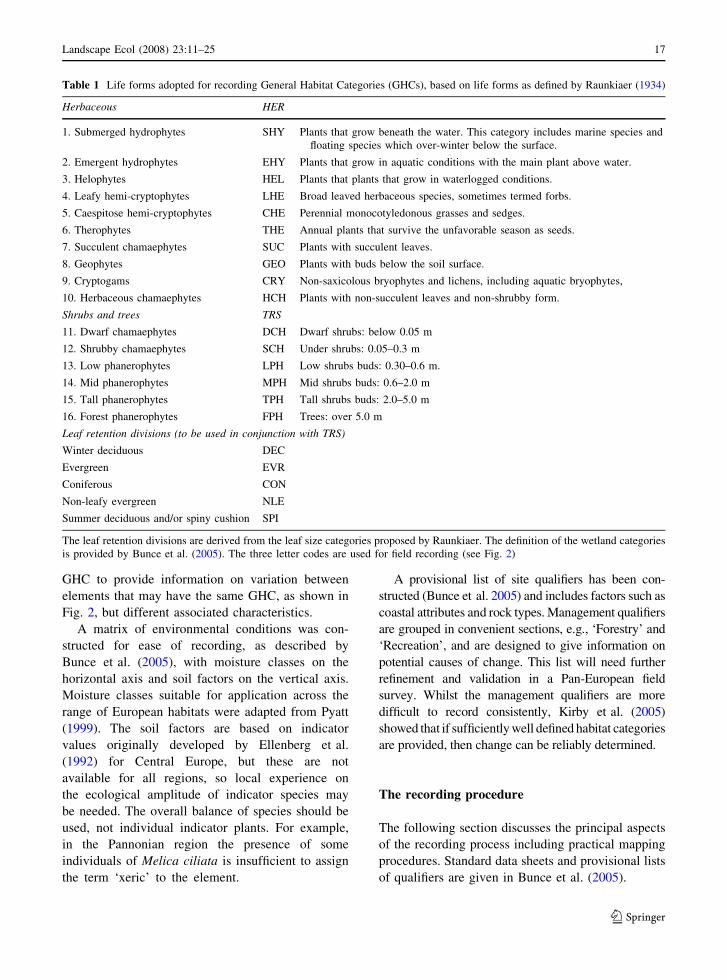
Land associated with built structures and infrastruc-

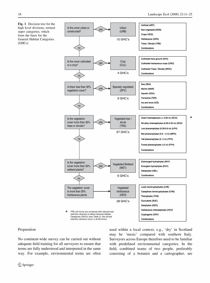
ture (termed ‘Urban’ in a broad sense) and agricultural

cropland (termed ‘Crops’) cannot be defined solely in

terms of life forms. However, for policy and practical

reasons it is essential that such land is identified.

Hence, ‘Urban’ and Crops’ have been separated as

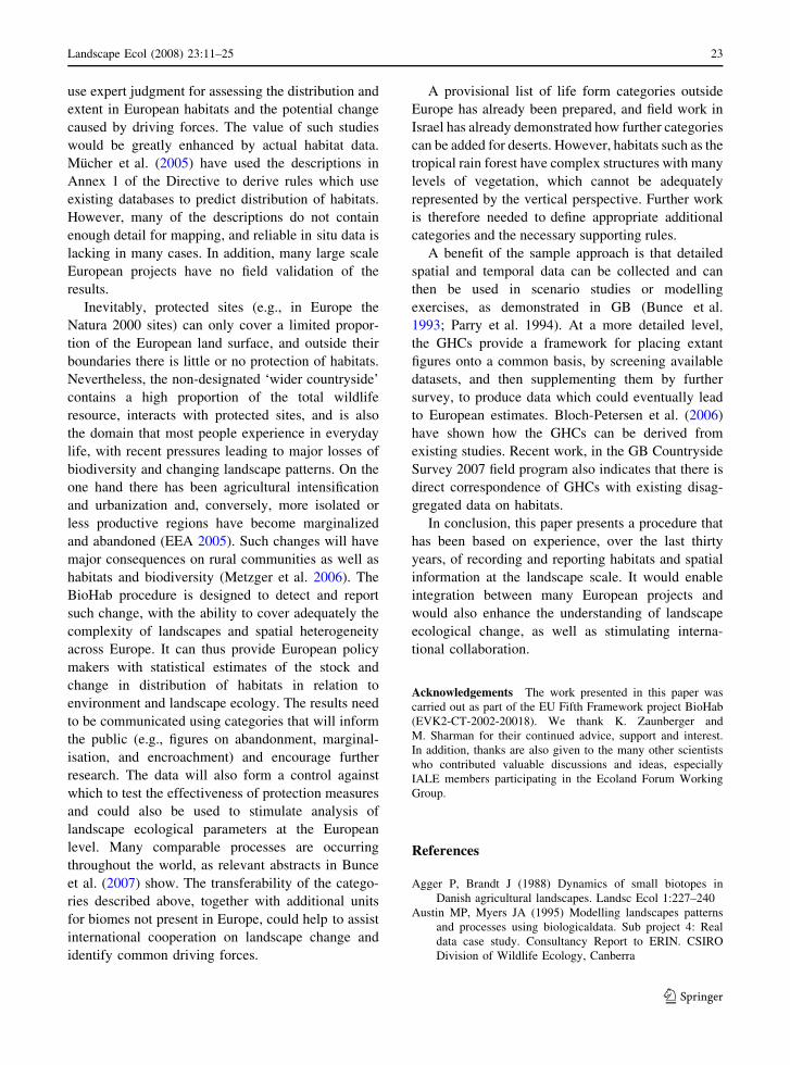
‘super categories’ at the first level of the hierarchy, as

shown in Fig. 1, with the rules to identify them being

provided by Bunce et al. (2005). However, within the

‘Crop’ and ‘Urban’ categories, subsequent divisions

are then based on life forms at the second level of

Fig. 1. In addition, the ‘Sparsely Vegetated’ super

category is separated to cover land with vegetation

cover below 30%; e.g., glacial moraines.

A major problem of using theoretical habitat

classifications for monitoring is the proliferation of

classes; e.g., Morillo Fernandez (2003) distinguished

almost 1,000 classes and in EUNIS there are 350

classes at level three. Within the BioHab, as shown in

Fig. 1, all possible feasible combinations of grouped

pairs of life forms are included, to ensure complete

coverage of Europe. The number is restricted by rules

using percentages and prioritisation to exclude com-

binations which would include more than two life

forms. For ‘Trees and Shrubs’ leaf retention divisions

are also included, but not all of these are present in all

height categories; e.g., there are no native Summer

Deciduous trees over five metres in height in Europe.

This procedure is arbitrary, but reproducible, and has

restricted the number of GHCs to 130 in the Pan-

European region, excluding Turkey. Other life forms,

e.g., tall succulents, would have to be included for other

continents. This restricted list acts as a lowest common

denominator and enables decisions at the highest level

to be made in the field, or to be derived from extant data

(e.g., vegetation relevees). More detailed information

(see below) is recorded in subsequent columns for the

interpretation of change at the landscape level.

The determination of the GHC is based upon a

series of five dichotomous divisions as shown in

Fig. 1. These determine the set of life forms that can

be used to identify the appropriate GHC. The first

decision concerns whether the element is ‘Urban’, the

second whether it is a ‘Crop’, the third whether it is

‘Sparsely Vegetated’, the fourth whether it is ‘Trees

or Shrubs’, and the fifth whether it is ‘Wetland’

(Fig. 1). As discussed below, rules have then been

added for further divisions in all super categories and

habitat categories, including percentage criteria.

Additional qualifiers

Additional qualifiers are essential for further descrip-

tion of the GHCs and the determination of landscape

ecological characteristics. Lists of global (e.g., per-

centage cover), environmental (e.g., soil moisture),

site (e.g., moraine) and management (e.g., cattle

grazing) qualifiers have been constructed. These

qualifiers are recorded in combination with the

16 Landscape Ecol (2008) 23:11–25

123

GHC to provide information on variation between

elements that may have the same GHC, as shown in

Fig. 2, but different associated characteristics.

A matrix of environmental conditions was con-

structed for ease of recording, as described by

Bunce et al. (2005), with moisture classes on the

horizontal axis and soil factors on the vertical axis.

Moisture classes suitable for application across the

range of European habitats were adapted from Pyatt

(1999). The soil factors are based on indicator

values originally developed by Ellenberg et al.

(1992) for Central Europe, but these are not

available for all regions, so local experience on

the ecological amplitude of indicator species may

be needed. The overall balance of species should be

used, not individual indicator plants. For example,

in the Pannonian region the presence of some

individuals of Melica ciliata is insufficient to assign

the term ‘xeric’ to the element.

A provisional list of site qualifiers has been con-

structed (Bunce et al. 2005) and includes factors such as

coastal attributes and rock types. Management qualifiers

are grouped in convenient sections, e.g., ‘Forestry’ and

‘Recreation’, and are designed to give information on

potential causes of change. This list will need further

refinement and validation in a Pan-European field

survey. Whilst the management qualifiers are more

difficult to record consistently, Kirby et al. (2005)

showed that if sufficiently well defined habitat categories

are provided, then change can be reliably determined.

The recording procedure

The following section discusses the principal aspects

of the recording process including practical mapping

procedures. Standard data sheets and provisional lists

of qualifiers are given in Bunce et al. (2005).

Table 1 Life forms adopted for recording General Habitat Categories (GHCs), based on life forms as defined by Raunkiaer (1934)

Herbaceous HER

1. Submerged hydrophytes SHY Plants that grow beneath the water. This category includes marine species and

floating species which over-winter below the surface.

2. Emergent hydrophytes EHY Plants that grow in aquatic conditions with the main plant above water.

3. Helophytes HEL Plants that plants that grow in waterlogged conditions.

4. Leafy hemi-cryptophytes LHE Broad leaved herbaceous species, sometimes termed forbs.

5. Caespitose hemi-cryptophytes CHE Perennial monocotyledonous grasses and sedges.

6. Therophytes THE Annual plants that survive the unfavorable season as seeds.

7. Succulent chamaephytes SUC Plants with succulent leaves.

8. Geophytes GEO Plants with buds below the soil surface.

9. Cryptogams CRY Non-saxicolous bryophytes and lichens, including aquatic bryophytes,

10. Herbaceous chamaephytes HCH Plants with non-succulent leaves and non-shrubby form.

Shrubs and trees TRS

11. Dwarf chamaephytes DCH Dwarf shrubs: below 0.05 m

12. Shrubby chamaephytes SCH Under shrubs: 0.05–0.3 m

13. Low phanerophytes LPH Low shrubs buds: 0.30–0.6 m.

14. Mid phanerophytes MPH Mid shrubs buds: 0.6–2.0 m

15. Tall phanerophytes TPH Tall shrubs buds: 2.0–5.0 m

16. Forest phanerophytes FPH Trees: over 5.0 m

Leaf retention divisions (to be used in conjunction with TRS)

Winter deciduous DEC

Evergreen EVR

Coniferous CON

Non-leafy evergreen NLE

Summer deciduous and/or spiny cushion SPI

The leaf retention divisions are derived from the leaf size categories proposed by Raunkiaer. The definition of the wetland categories

is provided by Bunce et al. (2005). The three letter codes are used for field recording (see Fig. 2)

Landscape Ecol (2008) 23:11–25 17

123

Preparation

No continent-wide survey can be carried out without

adequate field training for all surveyors to ensure that

terms are fully understood and interpreted in the same

way. For example, environmental terms are often

used within a local context, e.g., ‘dry’ in Scotland

may be ‘mesic’ compared with southern Italy.

Surveyors across Europe therefore need to be familiar

with predefined environmental categories. In the

field, combined teams of two people, preferably

consisting of a botanist and a cartographer, are

yes

Is the cover urban orconstructed?

Is the cover cultivatedor a crop?

Is there less than 30%vegetation cover?

Is the vegetationcover more than 30%trees or shrubs?

Is the vegetationcover more than 30%wetland plants?

yes

yes

yes

no

no

no

no

Urban(URB)

Crop(CUL)

Sparsely vegetated(SPV)

Vegetated tree /shrub(TRS)

Vegetated Wetland(WET)

Combinations

Trees / Shrubs (TRE)

Herbaceous (GRA)

Crops (VEG)

Non-vegetated (NON)

Artificial (ART)

Combinations

Trees / Shrubs (TRE)

Herbaceous (GRA)

Crops (VEG)

Non-vegetated (NON)

Artificial (ART)

Combinations

Cultivated Trees / Shrubs (WOC)

Cultivated herbaceous crops (CRO)

Cultivated bare ground (SPA)

Combinations

Cultivated Trees / Shrubs (WOC)

Cultivated herbaceous crops (CRO)

Cultivated bare ground (SPA)

Combinations

Ice and snow (ICE)

Terrestrial (TER)

Aquatic (AQU)

Marine (MAR)

Sea (SEA)

Combinations

Ice and snow (ICE)

Terrestrial (TER)

Aquatic (AQU)

Marine (MAR)

Sea (SEA)

Combinations

Helophytes (HEL)

Emergent hydrophytes (EHY)

Submerged hydrophytes (SHY)

Combinations

Helophytes (HEL)

Emergent hydrophytes (EHY)

Submerged hydrophytes (SHY)

Forest phanerophytes (>5 m) (FPH)

Combinations

Tall phanerophytes (2- 5 m) (TPH)

Mid phanerophytes (0.6 – 2 m) (MPH)

Low phanerophytes (0.30-0.6 m) (LPH)

Shrubby chamaephytes (0.05-0.30 m) (SCH)

Dwarf chamaephytes (< 0.05 m) (DCH)

Forest phanerophytes (>5 m) (FPH)

Combinations

Tall phanerophytes (2- 5 m) (TPH)

Mid phanerophytes (0.6 – 2 m) (MPH)

Low phanerophytes (0.30-0.6 m) (LPH)

Shrubby chamaephytes (0.05-0.30 m) (SCH)

Dwarf chamaephytes (< 0.05 m) (DCH)

15 GHC’s

4 GHC’s

9 GHC’s

67 GHC’s

6 GHC’s

The vegetation coveris more than 30%herbaceous plants

Vegetatedherbaceous

(HER)

Combinations

Cryptogams (CRY)

Herbaceous chamaephytes (HCH)

Geophytes (GEO)

Succulents (SUC)

Therophytes (THE)

Caespitose hemicryptophytes (CHE)

Leafy hemicryptophytes (LHE)

Combinations

Cryptogams (CRY)

Herbaceous chamaephytes (HCH)

Geophytes (GEO)

Succulents (SUC)

Therophytes (THE)

Caespitose hemicryptophytes (CHE)

Leafy hemicryptophytes (LHE)

28 GHC’s

yes

no

TRS Life forms are combined with relevant leafretention divisions to define General HabitatCategories (GHCs) (see Table 2). Not all leafretention divisions occur in all life forms.

*

*

Fig. 1 Decision tree for the

high level divisions, termed

super categories, which

form the basis for the

General Habitat Categories

(GHCs)

18 Landscape Ecol (2008) 23:11–25

123

needed to ensure that the necessary expertise is

available.

The date for the recording of GHCs should be

based on local phenology. The extent of the window

needs to be set by region, using local information,

and differs between environmental zones. The state

of development of the vegetation at the recording

date should therefore be relatively consistent

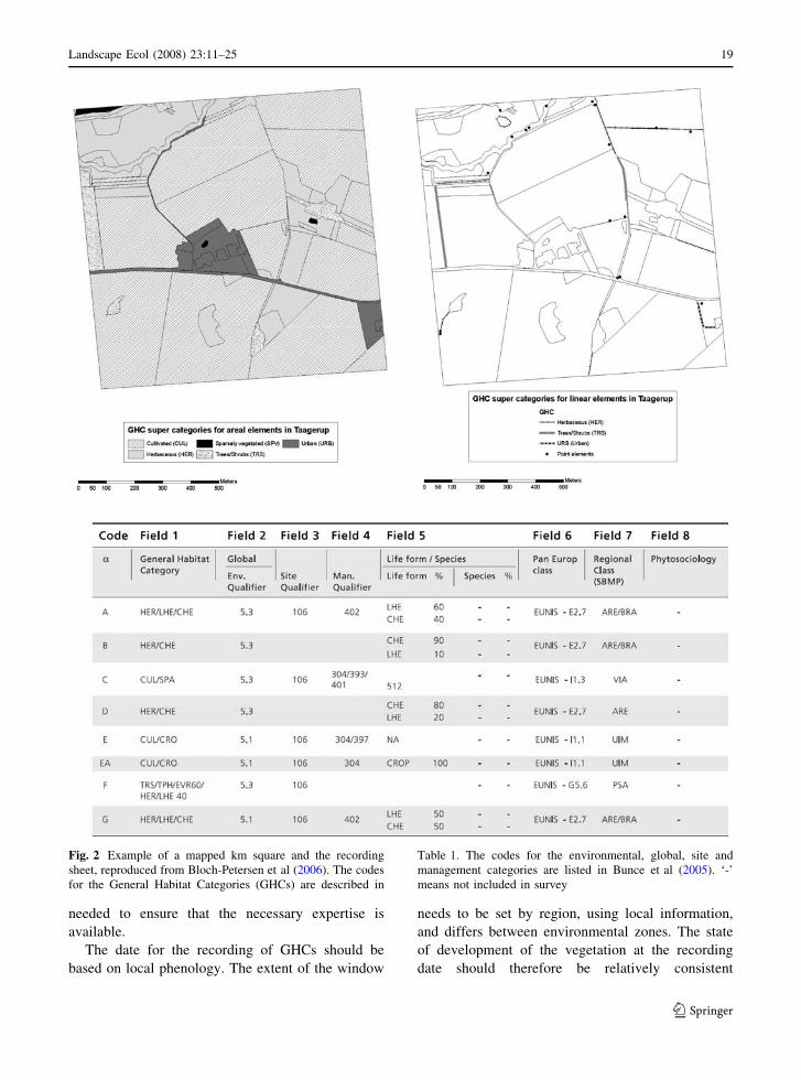
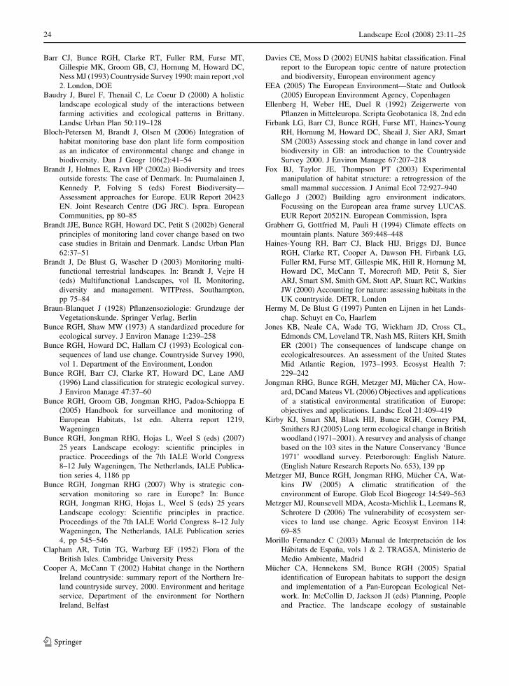
Fig. 2 Example of a mapped km square and the recording

sheet, reproduced from Bloch-Petersen et al (2006). The codes

for the General Habitat Categories (GHCs) are described in

Table 1. The codes for the environmental, global, site and

management categories are listed in Bunce et al (2005). ‘-’

means not included in survey

Landscape Ecol (2008) 23:11–25 19

123

between zones; thus in the Mediterranean region the

recording period will be earlier than in central and

northern Europe. Barr et al. (1993) showed that

differences between dates of survey are a major

source of noise in change statistics. Repeat visits for

monitoring should therefore be carried out as close

as possible to the date of the original visit,

assuming that there is no shift in timings of the

seasons.

Data quality control (i.e., supervision of surveyors)

and assurance (i.e., independent checks of recording)

are all essential to produce robust data. Barr et al.

(1993) analyzed random checks of comparable cat-

egories to GHCs and showed a correspondence of

84%. Any future program would need to incorporate

such checks, so that policy makers and scientists

would have confidence in the results.

All major decisions are made in the field. At a

later stage, it is possible to extract relevant data in

the laboratory from available datasets (e.g., slope

angles, and geology). Other more detailed data are

added in the field, as described below. Brandt et al.

(2002) emphasize that the quality of mapping is

dependent on sufficiently accurate base maps. It is

therefore preferable to carry out preparatory work

on ecological interpretation and subsequent delinea-

tion of the major elements within the survey area

from aerial photographs and related material, e.g.,

cadastral maps, preferably at a 1:10,000 scale.

Surveyors therefore annotate the base map with

labels attached to individual elements according to

the rules. The boundaries of some elements may

need to be adjusted or new parcels described which

were not defined in the preparatory work, e.g.,

different categories of grassland can often not be

seen on aerial photographs.

Areal elements

The procedure was initially developed for mapping

1 km square samples, but is also suitable for other

scales, e.g.; Cooper and McCann (2002) used

0.25 km squares and Bloch-Petersen et al. (2006)

applied the GHCs to small biotopes below about

200 m2. Within the 1 km square sample unit, the

surveyor delineates all habitats with an area greater

than 400 m2 (Minimal Mappable Element - MME).

Figure 2 gives an example of a mapped 1 km square

and a recording sheet (Bloch-Petersen et al. 2006).

For each delineated unit the surveyor determines the

GHC (Field 1) and the environmental, site, and

management qualifiers, which are in sequential fields

on the recording sheet (Fields 2–4). Next, all life

forms with a cover of over 10% are recorded and

individual plant species or crops with a cover of over

30% in the mapping unit (Field 5). Three further

fields are provided for existing Pan-European habitat

classifications (e.g., EUNIS (Davies and Moss

(2002)), national habitat classifications (e.g. (Morillo-

Fernandez 2003) and phytosociological associations

(e.g., Rodwell et al. 2002) depending upon the

objectives of the project and the experience of the

surveyors.

Although the MME has to occupy at least 400 m2

it can be a complex shape, so long as the shortest

measurement is over 5 m, as in the GB Countryside

Survey, and checked for Europe during BioHab.

This contrasts with the 10,000 m2 of the CORINE

land cover map and 2,500 m2 of the Biopress

Project (Olschofsky et al. 2006). However, the finer

detail of the MME is essential to express the

landscape ecological characteristics of small scale

landscapes; e.g., in Crete (Greece), Asturias (Spain),

and Brittany (France). Bunce et al. (2005) provide

detailed rules for mapping some elements, e.g.,

motorways will be mapped as areal elements, but

may subsequently be allocated to linear features by

database management for specific objectives (e.g.,

Haines-Young et al. 2000). The fundamental princi-

ple is that disaggregated data are collected, so that

subsequent analyses can be sufficiently flexible to

answer a variety of policy and landscape ecological

objectives, e.g., loss of hedgerows and fragmenta-

tion of habitats.

Linear and point elements

Linear and point elements are often excluded from

habitat surveys. However, many landscape ecological

studies have shown that, especially in intensively

managed agricultural landscapes, biodiversity has

progressively become restricted to such features (e.g.,

Hermy and De Blust 1997). Whilst this process may

have stabilized in Western Europe, it is likely to

continue in Central Europe. Many cultural landscapes

are rich in such features, largely as a result of

20 Landscape Ecol (2008) 23:11–25

123

management; e.g., terraces in Tuscany (Italy), walls

in the Auvergne (France) and ponds in Cheshire

(GB). It is therefore essential not only to assess the

resources of linear and point elements in representa-

tive landscapes but also to monitor their patterns and

change.

The same recording format as described in the

previous section is used for linear and point elements,

but on a separate sheet, in order to assist the recording

process. The variation across different types of

landscape can subsequently be integrated through

the use of Geographical Information Systems (GIS),

and the contribution to biodiversity of areal, linear

and point features compared. In some projects, e.g.,

Cooper and McCann (2002) habitats only may be

recorded, but data on other biota may also be

collected in the same sites, e.g., vegetation and

freshwater invertebrates (Haines-Young et al. (2000))

in order to present an integrated picture of biodiver-

sity at the landscape scale.

Linear elements have a Minimal Mappable Length

(MML) of 30 m. Those features that comprise only

vegetation must be wider than 0.5 m, but less than

5 m wide in order to exclude narrow strips (e.g., lines

of vegetation beside walls). Elements that are smaller

than 400 m2 and shorter than 30 m can be recorded as

points. Linear habitats often occur as complexes; e.g.,

a fence, a ditch and a hedge; in which case

instructions are provided for mapping, so that a given

combination is always recorded by single alpha-

numeric code incorporating its detailed composition.

In some cultural landscapes the number of point

features can be large, e.g., individual trees in

parkland or hedgerows. Two guidelines are provided

for recording such points. Firstly, the recorded point

features should add to landscape diversity, usually

because they represent a particular habitat which is

generally absent from the surrounding area, e.g., rock

outcrops or boulders in a grass field. Secondly, the

recorded point features should also have an effect on

the ecological functioning of landscapes, e.g., small

water bodies which act as drinking places in grass-

lands, or weirs in watercourses, which hinder

migration of fish. However, a given survey may

decide to omit point features, in which case this

should be documented on the separate general

information sheet, which also includes information

such as the date of survey and ownership details

(Bunce et al. 2005).

Discussion

Field testing and validation

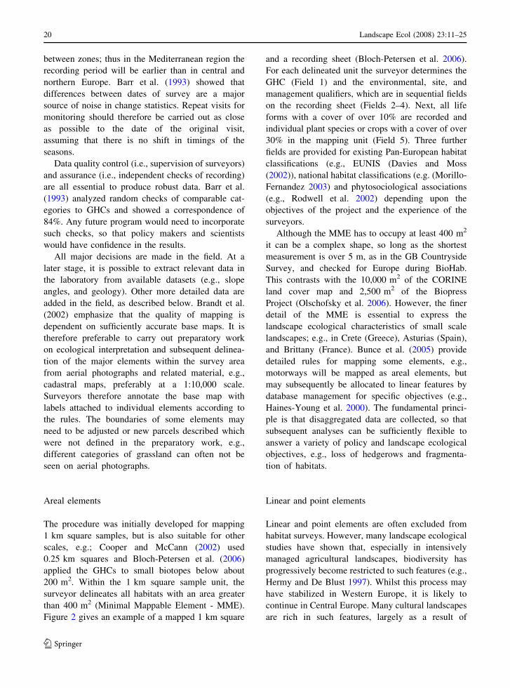
It was essential to ensure that the categories and rules

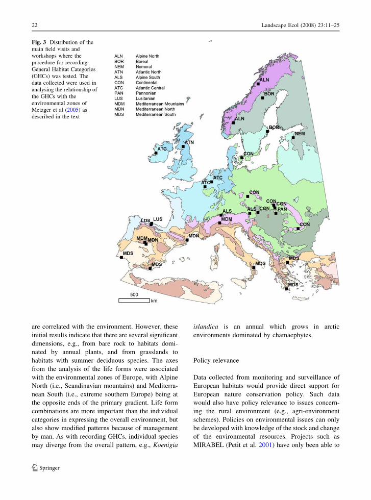
could be applied throughout Europe. The field

procedure was therefore tested rigorously through

excursions and field workshops to bio-geographical

locations ranging from the desert of Tabernas, near

Almeria (Spain), to northern Norway inside the

Arctic Circle (Fig. 3). These sites were selected to

ensure that GHCs covered all major life forms and

environmental conditions, and that the mapping rules

were sufficiently robust. The categories and rules

were progressively refined during these visits. In

addition, the exposure of the mapping procedures to

external comments was also valuable and led to

modifications to the original proposal. Whilst some

categories are rare and may never reach an MME or

MML, the inclusion of point features enables the

comprehensive expression of variation within the

landscape.

The theoretical basis of the model is the correla-

tion between the complexes of life forms and the

environment. It is the substance of classical bioge-

ography and can therefore be tested. The first such

test was carried out in a valley in the Picos de Europa

(Spain) which extends from evergreen forest at

200 m to rock and sub-alpine habitats at 2,500 m.

Orthogonal regression, as described by Bunce et al.

(1996), was used to calculate the correlation between

Detrended Correspondence Analysis (DCA) scores of

the mixtures of plant life forms recorded in 80

stratified random samples of 0.25 km square, drawn

from eight environmental strata, using the mean

altitude of each stratum as the independent variable.

The correlation coefficient was 0.94 (6 df) and highly

significant (P \ 0.001) showing that the model is

valid.

In the second test, the data used was for proportion

of life forms in areal elements collected during the

field excursions and workshops shown in Fig. 3. The

results are only indicative because, although they

include all environmental zones of Europe, they were

not randomly stratified. The data were analyzed by

Canonical Correspondence Analysis using the envi-

ronmental zones as the independent variable

(Metzger et al. 2005). The results confirm the

hypothesis of Raunkiaer (1934) that life form spectra

Landscape Ecol (2008) 23:11–25 21

123

are correlated with the environment. However, these

initial results indicate that there are several significant

dimensions, e.g., from bare rock to habitats domi-

nated by annual plants, and from grasslands to

habitats with summer deciduous species. The axes

from the analysis of the life forms were associated

with the environmental zones of Europe, with Alpine

North (i.e., Scandinavian mountains) and Mediterra-

nean South (i.e., extreme southern Europe) being at

the opposite ends of the primary gradient. Life form

combinations are more important than the individual

categories in expressing the overall environment, but

also show modified patterns because of management

by man. As with recording GHCs, individual species

may diverge from the overall pattern, e.g., Koenigia

islandica is an annual which grows in arctic

environments dominated by chamaephytes.

Policy relevance

Data collected from monitoring and surveillance of

European habitats would provide direct support for

European nature conservation policy. Such data

would also have policy relevance to issues concern-

ing the rural environment (e.g., agri-environment

schemes). Policies on environmental issues can only

be developed with knowledge of the stock and change

of the environmental resources. Projects such as

MIRABEL (Petit et al. 2001) have only been able to

Fig. 3 Distribution of the

main field visits and

workshops where the

procedure for recording

General Habitat Categories

(GHCs) was tested. The

data collected were used in

analysing the relationship of

the GHCs with the

environmental zones of

Metzger et al (2005) as

described in the text

22 Landscape Ecol (2008) 23:11–25

123

use expert judgment for assessing the distribution and

extent in European habitats and the potential change

caused by driving forces. The value of such studies

would be greatly enhanced by actual habitat data.

Mucher et al. (2005) have used the descriptions in

Annex 1 of the Directive to derive rules which use

existing databases to predict distribution of habitats.

However, many of the descriptions do not contain

enough detail for mapping, and reliable in situ data is

lacking in many cases. In addition, many large scale

European projects have no field validation of the

results.

Inevitably, protected sites (e.g., in Europe the

Natura 2000 sites) can only cover a limited propor-

tion of the European land surface, and outside their

boundaries there is little or no protection of habitats.

Nevertheless, the non-designated ‘wider countryside’

contains a high proportion of the total wildlife

resource, interacts with protected sites, and is also

the domain that most people experience in everyday

life, with recent pressures leading to major losses of

biodiversity and changing landscape patterns. On the

one hand there has been agricultural intensification

and urbanization and, conversely, more isolated or

less productive regions have become marginalized

and abandoned (EEA 2005). Such changes will have

major consequences on rural communities as well as

habitats and biodiversity (Metzger et al. 2006). The

BioHab procedure is designed to detect and report

such change, with the ability to cover adequately the

complexity of landscapes and spatial heterogeneity

across Europe. It can thus provide European policy

makers with statistical estimates of the stock and

change in distribution of habitats in relation to

environment and landscape ecology. The results need

to be communicated using categories that will inform

the public (e.g., figures on abandonment, marginal-

isation, and encroachment) and encourage further

research. The data will also form a control against

which to test the effectiveness of protection measures

and could also be used to stimulate analysis of

landscape ecological parameters at the European

level. Many comparable processes are occurring

throughout the world, as relevant abstracts in Bunce

et al. (2007) show. The transferability of the catego-

ries described above, together with additional units

for biomes not present in Europe, could help to assist

international cooperation on landscape change and

identify common driving forces.

A provisional list of life form categories outside

Europe has already been prepared, and field work in

Israel has already demonstrated how further categories

can be added for deserts. However, habitats such as the

tropical rain forest have complex structures with many

levels of vegetation, which cannot be adequately

represented by the vertical perspective. Further work

is therefore needed to define appropriate additional

categories and the necessary supporting rules.

A benefit of the sample approach is that detailed

spatial and temporal data can be collected and can

then be used in scenario studies or modelling

exercises, as demonstrated in GB (Bunce et al.

1993; Parry et al. 1994). At a more detailed level,

the GHCs provide a framework for placing extant

figures onto a common basis, by screening available

datasets, and then supplementing them by further

survey, to produce data which could eventually lead

to European estimates. Bloch-Petersen et al. (2006)

have shown how the GHCs can be derived from

existing studies. Recent work, in the GB Countryside

Survey 2007 field program also indicates that there is

direct correspondence of GHCs with existing disag-

gregated data on habitats.

In conclusion, this paper presents a procedure that

has been based on experience, over the last thirty

years, of recording and reporting habitats and spatial

information at the landscape scale. It would enable

integration between many European projects and

would also enhance the understanding of landscape

ecological change, as well as stimulating interna-

tional collaboration.

Acknowledgements The work presented in this paper was

carried out as part of the EU Fifth Framework project BioHab

(EVK2-CT-2002-20018). We thank K. Zaunberger and

M. Sharman for their continued advice, support and interest.

In addition, thanks are also given to the many other scientists

who contributed valuable discussions and ideas, especially

IALE members participating in the Ecoland Forum Working

Group.

References

Agger P, Brandt J (1988) Dynamics of small biotopes in

Danish agricultural landscapes. Landsc Ecol 1:227–240

Austin MP, Myers JA (1995) Modelling landscapes patterns

and processes using biologicaldata. Sub project 4: Real

data case study. Consultancy Report to ERIN. CSIRO

Division of Wildlife Ecology, Canberra

Landscape Ecol (2008) 23:11–25 23

123

Barr CJ, Bunce RGH, Clarke RT, Fuller RM, Furse MT,

Gillespie MK, Groom GB, CJ, Hornung M, Howard DC,

Ness MJ (1993) Countryside Survey 1990: main report ,vol

2. London, DOE

Baudry J, Burel F, Thenail C, Le Coeur D (2000) A holistic

landscape ecological study of the interactions between

farming activities and ecological patterns in Brittany.

Landsc Urban Plan 50:119–128

Bloch-Petersen M, Brandt J, Olsen M (2006) Integration of

habitat monitoring base don plant life form composition

as an indicator of environmental change and change in

biodiversity. Dan J Geogr 106(2):41–54

Brandt J, Holmes E, Ravn HP (2002a) Biodiversity and trees

outside forests: The case of Denmark. In: Puumalainen J,

Kennedy P, Folving S (eds) Forest Biodiversity—

Assessment approaches for Europe. EUR Report 20423

EN. Joint Research Centre (DG JRC). Ispra. European

Communities, pp 80–85

Brandt JJE, Bunce RGH, Howard DC, Petit S (2002b) General

principles of monitoring land cover change based on two

case studies in Britain and Denmark. Landsc Urban Plan

62:37–51

Brandt J, De Blust G, Wascher D (2003) Monitoring multi-

functional terrestrial landscapes. In: Brandt J, Vejre H

(eds) Multifunctional Landscapes, vol II, Monitoring,

diversity and management. WITPress, Southampton,

pp 75–84

Braun-Blanquet J (1928) Pflanzensoziologie: Grundzuge der

Vegetationskunde. Springer Verlag, Berlin

Bunce RGH, Shaw MW (1973) A standardized procedure for

ecological survey. J Environ Manage 1:239–258

Bunce RGH, Howard DC, Hallam CJ (1993) Ecological con-

sequences of land use change. Countryside Survey 1990,

vol 1. Department of the Environment, London

Bunce RGH, Barr CJ, Clarke RT, Howard DC, Lane AMJ

(1996) Land classification for strategic ecological survey.

J Environ Manage 47:37–60

Bunce RGH, Groom GB, Jongman RHG, Padoa-Schioppa E

(2005) Handbook for surveillance and monitoring of

European Habitats, 1st edn. Alterra report 1219,

Wageningen

Bunce RGH, Jongman RHG, Hojas L, Weel S (eds) (2007)

25 years Landscape ecology: scientific principles in

practice. Proceedings of the 7th IALE World Congress

8–12 July Wageningen, The Netherlands, IALE Publica-

tion series 4, 1186 pp

Bunce RGH, Jongman RHG (2007) Why is strategic con-

servation monitoring so rare in Europe? In: Bunce

RGH, Jongman RHG, Hojas L, Weel S (eds) 25 years

Landscape ecology: Scientific principles in practice.

Proceedings of the 7th IALE World Congress 8–12 July

Wageningen, The Netherlands, IALE Publication series

4, pp 545–546

Clapham AR, Tutin TG, Warburg EF (1952) Flora of the

British Isles. Cambridge University Press

Cooper A, McCann T (2002) Habitat change in the Northern

Ireland countryside: summary report of the Northern Ire-

land countryside survey, 2000. Environment and heritage

service, Department of the environment for Northern

Ireland, Belfast

Davies CE, Moss D (2002) EUNIS habitat classification. Final

report to the European topic centre of nature protection

and biodiversity, European environment agency

EEA (2005) The European Environment—State and Outlook

(2005) European Environment Agency, Copenhagen

Ellenberg H, Weber HE, Duel R (1992) Zeigerwerte von

Pflanzen in Mitteleuropa. Scripta Geobotanica 18, 2nd edn

Firbank LG, Barr CJ, Bunce RGH, Furse MT, Haines-Young

RH, Hornung M, Howard DC, Sheail J, Sier ARJ, Smart

SM (2003) Assessing stock and change in land cover and

biodiversity in GB: an introduction to the Countryside

Survey 2000. J Environ Manage 67:207–218

Fox BJ, Taylor JE, Thompson PT (2003) Experimental

manipulation of habitat structure: a retrogression of the

small mammal succession. J Animal Ecol 72:927–940

Gallego J (2002) Building agro environment indicators.

Focussing on the European area frame survey LUCAS.

EUR Report 20521N. European Commission, Ispra

Grabherr G, Gottfried M, Pauli H (1994) Climate effects on

mountain plants. Nature 369:448–448

Haines-Young RH, Barr CJ, Black HIJ, Briggs DJ, Bunce

RGH, Clarke RT, Cooper A, Dawson FH, Firbank LG,

Fuller RM, Furse MT, Gillespie MK, Hill R, Hornung M,

Howard DC, McCann T, Morecroft MD, Petit S, Sier

ARJ, Smart SM, Smith GM, Stott AP, Stuart RC, Watkins

JW (2000) Accounting for nature: assessing habitats in the

UK countryside. DETR, London

Hermy M, De Blust G (1997) Punten en Lijnen in het Lands-

chap. Schuyt en Co, Haarlem

Jones KB, Neale CA, Wade TG, Wickham JD, Cross CL,

Edmonds CM, Loveland TR, Nash MS, Riiters KH, Smith

ER (2001) The consequences of landscape change on

ecologicalresources. An assessment of the United States

Mid Atlantic Region, 1973–1993. Ecosyst Health 7:

229–242

Jongman RHG, Bunce RGH, Metzger MJ, Mucher CA, How-

ard, DCand Mateus VL (2006) Objectives and applications

of a statistical environmental stratification of Europe:

objectives and applications. Landsc Ecol 21:409–419

Kirby KJ, Smart SM, Black HIJ, Bunce RGH, Corney PM,

Smithers RJ (2005) Long term ecological change in British

woodland (1971–2001). A resurvey and analysis of change

based on the 103 sites in the Nature Conservancy ‘Bunce

1971’ woodland survey. Peterborough: English Nature.

(English Nature Research Reports No. 653), 139 pp

Metzger MJ, Bunce RGH, Jongman RHG, Mucher CA, Wat-

kins JW (2005) A climatic stratification of the

environment of Europe. Glob Ecol Biogeogr 14:549–563

Metzger MJ, Rounsevell MDA, Acosta-Michlik L, Leemans R,

Schrotere D (2006) The vulnerability of ecosystem ser-

vices to land use change. Agric Ecosyst Environ 114:

69–85

Morillo Fernandez C (2003) Manual de Interpretacion de los

Habitats de Espana, vols 1 & 2. TRAGSA, Ministerio de

Medio Ambiente, Madrid

Mucher CA, Hennekens SM, Bunce RGH (2005) Spatial

identification of European habitats to support the design

and implementation of a Pan-European Ecological Net-

work. In: McCollin D, Jackson JI (eds) Planning, People

and Practice. The landscape ecology of sustainable

24 Landscape Ecol (2008) 23:11–25

123

landscapes. Proceedings of the 13th annual IALE

(UK) conference, 2005

New JR (2000) How useful are ant assemblages in monitoring

habitat disturbance in grasslands in south-east Australia. J

Insect Conserv 4:153–159

Oberdorfer E, Muller T, Korneck D, Lippert W, Markgraf-

Dannenberg I (1990) Pflanzensoziologische Exkursionsflora.

6th edn. Stuttgart Ulmer

Olschofsky K, Kohler R, Gerard F (2006) Land cover change

in Europe from the 1950’ies to 2000, aerial photo inter-

pretation and derived statistics from 59 samples

distributed across Europe. World Forestry, Hamburg

Parry ML, Hossell JE, Jones PJ, Rehman T, Tranter RB, Marsh

JS, Rosenzweig C, Fischer G, Carson LG, Bunce RGH

(1996) Integrating global and regional analyses of the

effects of climate change: a case study of land use in

England and Wales. Clim Change 32:185–198

Petit S, Firbank L, Wyatt B, Howard D (2001) MIRABEL,

Models for integrated assessment of biodiversity in

European landscapes. AMBIO 30:81–88

Petit S, Griffiths L, Smart S, Smith GM, Stuart RC, Wright SM

(2004) Effects of area and isolation of woodland patches

on herbaceous plant species richness in Great Britain.

Landsc Ecol 19:463–471

Pyatt DG (1999) Correlation of European forest site classifi-

cations. EU Concerted action final report, Forest research

northern station, Roslin

Quezel P, Barbero M (1982) Definition and characterization of

Mediterranean-type ecosystems. Ecol Mediterr 7:15–29

Raunkiaer C (1934) The life forms of plants and statistical

plant geography, being the collected papers of C Raun-

kiaer. Clarendon, Oxford

Reid WV (2005) Millennium ecosystem assessment synthesis

report. Island Press, Washington DC, USA

Rodwell JS, Schaminee JHJ, Mucina L, Pignatti S, Dring J,

Moss D (2002) The Diversity of European Vegetation. An

overview of phytosociological alliances and their rela-

tionships to EUNIS habitats. Ministry of agriculture

nature management and fisheries, The Netherlands and

European environmental agency, 168 pp

Sheail J, Bunce RGH (2003) The development and scientific

principles of an environmental classification for strategic

ecological survey in Great Britain. Environ Conserv

30:147–159

Sitch S, Smith B, Prentice IC, Arneth A, Bondeau A, Cramer

W, Kaplan JO, Levis S, Lucht W, Sykes MT, Thonicke K,

Venevsky S, (2003) Evaluation of ecosystem dynamics,

plant geography and terrestrial carbon cycling in the LPJ

dynamic global vegetation model. Glob Chang Biol

9:161–185

Skanes H (1996) Landscape change and grassland dynamics—

retrospective studies based on aerial photographs and old

cadastral maps during 200 years in south Sweden. The

Department of Physical Geography, Stockholm Univer-

sity. Dissertation series, no. 8

Vogelman JE, Howard SM, Yang L, Larsen CR, Wylie BK,

van Driel (2001) Completion of the 1990s national hard

cover data set for the conterminous United States from

Landsat Thematic Mapper data and other sources. Pho-

togramm Eng Remote Sens 67:650–662

Woodward FI, Rochefort L (1991) Sensitivity analysis of

vegetation diversity to environmental change. Glob Ecol

Biogeogr Lett 1:7–23

Landscape Ecol (2008) 23:11–25 25

123