DEPARTMENT OF ENVIRONMENTAL PROTECTION Bureau of Water Standards and Facility Regulation

DOCUMENT NUMBER: 391-3200-015 TITLE: Standardized Biological Field Collection and Laboratory Methods EFFECTIVE DATE: Upon publication of notice as final in the Pennsylvania Bulletin AUTHORITY: Pennsylvania Department of Environmental Protection (DEP), Bureau of

Water Standards and Facility Regulation, Division of Water Quality Standards.

POLICY: This guidance provides the established procedures to collect and process

aquatic biological field data for lakes and streams data. PURPOSE: The guidance was developed to establish and standardize DEP’s

procedures for aquatic biological data collection methods. APPLICABILITY: This guidance applies to DEP staff that needs to conduct biological water

quality surveys. DISCLAIMER: The policies and procedures outlined in this guidance are intended to

supplement existing requirements. Nothing in the policies or procedures shall affect regulatory requirements.

The policies and procedures herein are not an adjudication or a regulation.

There is no intent on the part of DEP to give the rules in these policies that weight or deference. This document establishes the framework within which DEP will exercise its administrative discretion in the future. DEP reserves the discretion to deviate from this policy statement if circumstances warrant.

PAGE LENGTH: 67 pages LOCATION: Volume 30, Tab 12

391-3200-015 / DRAFT May 20, 2006 / Page i

TABLE OF CONTENTS

PAGE I. INTRODUCTION ...........................................................................................................................1 II. COLLECTOR’S PERMIT REQUIREMENTS...............................................................................2 III. STATION SELECTION CONSIDERATIONS..............................................................................3 IV. HABITAT ASSESSMENT .............................................................................................................7 V. BENTHIC MACROINVERTEBRATES ........................................................................................9 A. Net Mesh Considerations.....................................................................................................9 B. Qualitative Methods.............................................................................................................9 1. Kick-Screen............................................................................................................10 a. Traditional Method ....................................................................................10 b. Assessment Method ...................................................................................12 2. D-Frame .................................................................................................................12 C. Semi-Quantitative Method – PaDEP-RBP ........................................................................12 1. Sample Collection..................................................................................................13 2. Sample Processing .................................................................................................13 D. Quantitative Methods.........................................................................................................16

1. Surber-Type Samplers ...........................................................................................16 2. Multi-plate Samplers..............................................................................................17 3. Grab Samplers........................................................................................................17

E. Identification ......................................................................................................................18

1. Taxonomic Level ...................................................................................................18 2. Verifications...........................................................................................................18 3. Sample Retention ...................................................................................................19

VI. FISHES ..........................................................................................................................................21 A. Electrofishing Considerations............................................................................................21

1. Electrofishing Gear ................................................................................................21 B. Qualitative Fish Methods...................................................................................................22

1. Small (Wadeable) Stream Methods .......................................................................22 2. Large River, Lake, Pond Methods .........................................................................22

3. Fish Identification ..................................................................................................23 4. Record Keeping .....................................................................................................23

C. Quantitative Fish Methods.................................................................................................23 1. Peterson (Mark-Recapture) Method ......................................................................24

2. Zippen (Removal) Method.....................................................................................25

391-3200-015 / DRAFT May 20, 2006 / Page ii

3. Index of Biotic Integrity (IBI) Assessment Collection Protocol ...........................26

D. Fish Tissue Sampling Methods..........................................................................................30 VII. OTHER BIOLOGICAL SAMPLING METHODS.......................................................................33 A. Lake Specific Methods ......................................................................................................33 1. Plankton Sampling Method (Modified Standard Method 1002a)..........................33 2. Chlorophyll-a Sampling Method ...........................................................................34 B. Bacteriological Sampling Method .....................................................................................34 1. Sampling Frequency and Duration ........................................................................35 2. Sampling Design....................................................................................................35 3 Equipment ..............................................................................................................36 4. Sample Collection Methodology ...........................................................................36 5. Quality Control ......................................................................................................37 6. Laboratory Results .................................................................................................37 7. Data Processing......................................................................................................37 C. Periphyton Sampling Method ............................................................................................38 VIII. SAMPLING GEAR CHECKLIST ................................................................................................39 IX. TAXONOMY REFERENCE LIST...............................................................................................40 X. REFERENCES ..............................................................................................................................48 APPENDICES ...........................................................................................................................................49

391-3200-015 / DRAFT May 20, 2006 / Page iii

I. INTRODUCTION Aquatic organisms are excellent indicators of water quality and are routinely sampled as part of

Pennsylvania’s ongoing Water Quality Management (WQM) program. Expanding electronic data capability and increasing emphasis on quality assurance encouraged the Bureau of Water Standards and Facility Regulation (BWSFR) to develop these standardized benthic macroinvertebrate collection methods in 1988 (Standardized Biological Field Collection Methods, DER, 1988).

The 1988 manual presented field collection methods by the following survey types: qualitative

cause/effect surveys, quantitative cause/effect surveys, qualitative Water Quality Network (WQN) sampling, multi-plate sampling for cause/effect surveys, and WQN evaluations.

Changing trends in data management, bioassessment, the Antidegradation Program, and

biocriteria issues emphasized the need to revise the methods presented in the 1988 manual. In August 1995, these standardized methods were revised and updated. Since many of the methods/concepts used for each survey type overlap, the format has been changed to streamline the manual and reduce redundancy. In addition to the format change, the following procedures were added to these revisions:

• Sampling station selection • Qualitative Reference WQN sampling • Taxonomic quality assurance • Biological sample retention • Survey equipment checklist • Equipment maintenance schedules As the Department of Environmental Protection’s (DEP) water quality monitoring program

evolves to meet changing federal emphasis and requirements, it is apparent that this “Methods” manual must be a dynamic document - subject to improvements and revision in order to keep pace with advances in biological monitoring methodology. Since many advancements and program changes have occurred since 1995, the following items are updated or added:

• Station labeling (Sampling station selection section) • Statewide Surface Water Assessment kick screen method (Benthic Macroinvertebrate

Section) • Semi-quantitative method (PADEP-RBP) • Fish Index of Biotic Integrity (IBI) (Fish Section)

391-3200-015 / DRAFT May 20, 2006 / Page 1

II. COLLECTOR’S PERMIT REQUIREMENTS Field staff required to collect biological samples (particularly fish and benthic

macroinvertebrates) as part of their duties, must have a valid Collector’s Permit in their possession. Type II Collector Permits are issued annually by the Pennsylvania Fish & Boat Commission (PFBC)1 to state agency personnel (upon application) and require the possession of a current Pennsylvania fishing license.

Under normal circumstances, all DEP biologists that conduct field surveys independently on a

regular basis should be issued permits in their own name. Staff members that assist in field surveys only occasionally are not required to have their own permit, but must be listed on a permitted biologist’s Collector’s Permit as an assistant.

It shall be the biologist supervisors’ responsibility to ensure that their field staff obtain (and renew) their annual Collector’s Permit and the permittee’s responsibility to adhere to the rules and conditions of the permit.

1 For PFBC Collector’s Permits, contact: “Pennsylvania Fish & Boat Commission, Bureau of Administration, PO Box 67000, Harrisburg, PA 17106-7000”

391-3200-015 / DRAFT May 20, 2006 / Page 2

III. STATION SELECTION CONSIDERATIONS Station selection considerations are critically dependent on the type of survey to be conducted. Near-Field Investigations. Many traditional stream investigations are localized in their spatial

scope. They usually involve “above and below” sampling regimes that bracket suspected problem sources - necessitating background or traditional reference station comparisons (e.g., cause/effect surveys, pollution incidences or other impact surveys).

In order to limit the complications arising from compounding variables, select background

stations or reference waterbodies and impact stations that are physically similar in as many respects as possible. This includes matching drainage areas of similar size and setting. Substrate, depth, flow, gradient and aquatic plant growth should also be considered, as well as the location of tributaries, point source discharges and nonpoint source effects. A minimum of one background station must be selected, but select two if possible. Comparisons of background station(s) to impact station(s) include variation due to both natural and possible treatment (i.e., discharger) effects. An estimate of the natural variation sometimes can be made by comparing two background stations where the treatment effects are absent. A habitat assessment (Section IV) at each station may reveal physical limitations that would impact benthic communities.

Far-Field Investigations. Other stream investigations may involve much larger watershed or

basin-wide study areas. These would include water quality surveys designed to characterize overall impacts from land-use activities instead of specific discharges or localized pollution incidences. In these instances, station selection must discern between and adequately reflect all land-uses with potential impacts on water quality.

Examples include Antidegradation surveys and assessments conducted as part of the Statewide

Surface Waters Assessment Program. Generally, considerations listed above for “near-field” investigations may also be applicable to some far-field investigations, but certain reference or background station considerations may not apply. Antidegradation surveys do require “reference” comparisons, but since these stations are restricted to predetermined Exceptional Value (EV) watersheds, most of those selection considerations are already accounted for. The Statewide Surface Waters Assessment Program does not emphasize targeting “above and below” assessments of localized impact sources. The program does, however, accommodate assessment placement to distinguish point source impacts from nonpoint sources. In these cases, the assessments bracket the point source and become a near-field investigation for station selection purposes.

Station Length. Except for very small stream segments (<1-2 meter width), a station will

approximate a 100-meter reach. For the smaller segments, reaches of less than 100 meters can be considered, based on the biologist’s best professional judgment of how much stream length effectively characterizes that segment’s water quality condition.

Database Management. Much of the biological, chemical and physical data collected during

DEP’s numerous surveys is stored electronically, so it is important that the proper location information is recorded for each station surveyed. Such information provides reference points for data searches, retrievals, sorting and analyses. Once a station location has been determined, the following information should be recorded and provided in any resulting reports:

391-3200-015 / DRAFT May 20, 2006 / Page 3

• Stream Name - As recorded in the Pennsylvania Gazetteer of Streams. • Stream Code - A 5-digit number assigned to every named and unnamed stream in the

Commonwealth. • Latitude/Longitude - For electronic formats (Access database and Geographic

Information Systems (GIS)-based records), lat/long will be stored in decimal degrees. For maps, visual aids and report tables, lat/long can be reported in degrees - minutes-seconds,

based on U.S. Geological Survey (USGS) 7.5-minute quadrangle maps. They can be determined using lat/long gridded overlay sets, electronic digitizers or other similar devices.

• River Mile Index - The distance measured from the mouth upstream to the sampling

point and reported in 1/10th-mile increments. If sampling points are very close together, then the mileage may be reported in 1/100ths. Depending on the needed precision, map wheels or electronic measuring devices may be used.

• Narrative Description - A brief narration describing the station locations should be

provided; preferably in tabular form. Local landmarks, special features and road route numbers should be included when applicable. Include as many features as possible to aid in return visits by another investigator.

• Station Labeling - For new surveys that are not part of an already established, ongoing

monitoring program (i.e., WQN monitoring), sampled stations shall be labeled in the following manner:

1. All biological station data and stream segment data entered into DEP’s electronic

database will be assigned a specific code number known as a GISkey, which requires 15 characters to complete. The syntax format for a GISkey number follows a date-time-initials format: YYYYMMDD-0000-XYZ. This unique identification number is extremely important because it is used to reference and link all related forms, samples, computer records and GIS map images.

Date: Enter the assessment date in the following 8-digit format: YYYYMMDD

(e.g., 1/31/01 = 20010131); Time: Enter the time you begin filling out the form stream-side. Use the 4 digit

military format: 0000 (e.g., 8:30 AM = 0830; 8:30 PM = 2030). Leading zeros must be used for times < 10:00 AM;

Initials: Use the collector initials that are assigned to you. Newly hired staff must

contact the program manager or water quality database manager to receive their uniquely assigned collector initials before they begin any water quality assessments. Normally, these will be the three initials of the investigator’s full, legal name. In situations where the investigator has no middle initial or where initials duplicate those of another collector, unique collector initials will be assigned on a first-come-first-served basis.

391-3200-015 / DRAFT May 20, 2006 / Page 4

By following this GISkey format, each station will have its own unique identifier, distinguishing it from any other station in the database. Likewise, the same will be true for stream segment data. NOTE: Since the water quality data records are to be entered in the Access and ArcView GIS databases as distinctly separate entities in station and stream segment tables, it is OK for a station GISkey to match its stream segment GISkey.

2. For stream reporting narratives, discussion purposes, maps and visual aids, it is

desirable to use conventional station labels instead of a 15-digit GISkey. To facilitate a consistent station labeling method that encourages a logical comprehension of “upstream-downstream” cumulative water quality impacts, it is strongly suggested that the following guidelines be followed:

a. The stations will be labeled in hydrologic order, in upstream to

downstream order. b. The label will consist of a number followed by letter abbreviations of the

stream and tributary names. Refer to the following schematic diagram as an example and notice the labeling of two stream

names starting with the same letters:

MUDDY RIVER ⇓ Mill Creek unnamed 1MR →●

3MiC →● 7UNT→●

9PC→●

2PC→● ●←6PC

Pine Creek 8MoC→●

Morgan Creek 4LHR→● ●←5UNT 10MR →● Laurel Hardy Run unnamed

The ordering and labeling is within the context of the drainage basin or area studied. If the study

includes another basin entering Muddy River, then those stations would continue the sequence. For example, if another basin was studied in relation to the same project and it enters Muddy River downstream of 10MR, then its labeling sequence starts with “11”, beginning with the uppermost station. If there is another basin in your report, but it drains to a different receiving stream, a new sequence is used.

391-3200-015 / DRAFT May 20, 2006 / Page 5

This labeling system aids the report reader in tracing the presentation of data and information in hydrological order. Water chemistry, benthic and fish data tables should present the data columns numbered with the station labels in ascending order from left to right. When presented in this manner, background, cause/effect, chronic discharge and dilution influences on cumulative changes in water quality can be grasped more quickly. If any of these labeled stations are resurveyed in the future, it is suggested that the same station labels be used.

391-3200-015 / DRAFT May 20, 2006 / Page 6

IV. HABITAT ASSESSMENT DEP has adopted the habitat assessment methods outlined in the Environmental Protection

Agency’s (EPA) Rapid Bioassessment Protocols (RBP) (Plafkin, et al. 1989) and subsequently modified2. The matrix used to assess habitat quality is based on key physical characteristics of the waterbody and surrounding lands. All parameters evaluated represent potential limitations to the quality and quantity of instream habitat available to aquatic biota. These, in turn, affect community structure and composition.

The main purpose of the habitat assessment is to account for the limitations that are due to

existing stream conditions. This is particularly important in cause/effect and cumulative impact studies where the benthic community at any given station may already be self-limited by background watershed and habitat conditions or impacts from current land uses. In order to minimize the effects of habitat variability, every effort is made to sample similar habitats at all stations. The habitat assessment process involves rating 12 parameters2 as excellent, good, fair, or poor, by assigning a numeric value (ranging from 20 - 02), based on the criteria included on the Water Quality Network Habitat Assessment Riffle/Run Prevalence form (3800-FM-WSFR0402) and Habitat Assessment Field Data Sheet Glide Pool Prevalence form (3800-FM-WSFR0079) available on DEP’s Web site at www.depweb.state.pa.us .

The 12 habitat assessment parameters used in the PADEP-RBP evaluations for Riffle/Run

prevalent (and Glide/Pool prevalent) streams are discussed below. The Glide/Pool parameters that differ from the Riffle/Run parameters are shown in italics. The first four parameters evaluate stream conditions in the immediate vicinity of the benthic macroinvertebrate sampling point:

• Instream Fish Cover - Evaluates the percent makeup of the substrate (boulders, cobble,

other rock material) and submerged objects (logs, undercut banks) that provide refuge for fish.

• Epifaunal Substrate - Evaluates riffle quality, i.e., areal extent relative to stream width

and dominant substrate materials that are present. (In the absence of well-defined riffles, this parameter evaluates whatever substrate is available for aquatic invertebrate colonization.)

• Embeddedness - Estimates the percent (vertical depth) of the substrate interstitial spaces

filled with fine sediments. (Pool substrate characterization: evaluates the dominant type of substrate materials, i.e., gravel, mud, root mats, etc. that are more commonly found in glide/pool habitats.)

• Velocity/Depth Regime - Evaluates the presence/absence of four velocity/depth regimes -

fast-deep, fast-shallow, slow-deep and slow-shallow. (Generally, shallow is <0.5m and

2 Plafkin et al. originally presented nine habitat assessment parameters divided into three different scoring ranges of 20-0, 15-0, and 10-0. Modifications to these original habitat methods were presented at several seminars following this 1989 publication. These modifications added one more habitat parameter to each of the three original categories; bringing the total parameters to 12. The scoring ranges eventually were increased to 20-0 for all 12. This Habitat Protocol has undergone several more iterations - resulting in yet more variations from the original and DEP’s current 12 criteria - 20 point scoring habitat assessment method.

391-3200-015 / DRAFT May 20, 2006 / Page 7

slow is <0.3m/sec. Pool variability: describes the presence and dominance of several pool depth regimes.)

The next four parameters evaluate a larger area surrounding the sampled riffle. As a rule of

thumb, this expanded area is the stream length defined by how far upstream and downstream the investigator can see from the sample point.

• Channel Alteration - Primarily evaluates the extent of channelization or dredging but

can include any other forms of channel disruptions that would be detrimental to the habitat.

• Sediment Deposition - Estimates the extent of sediment effects in the formation of

islands, point bars and pool deposition. • Riffle Frequency (pool/riffle or run/bend ratio) - Estimates the frequency of riffle

occurrence based on stream width. (Channel sinuosity: the degree of sinuosity to total length of the study segment.)

• Channel Flow Status - Estimates the areal extent of exposed substrates due to water

level or flow conditions. The next four parameters evaluate an even greater area. This area is usually defined as the length

of stream that was electroshocked for fish (or an approximate 100-meter stream reach when no fish were sampled). It can also take into consideration upstream land-use activities in the watershed:

• Condition of Banks - Evaluates the extent of bank failure or signs of erosion. • Bank Vegetative Protection - Estimates the extent of stream bank that is covered by

plant growth providing stability through well-developed root systems. • Grazing or Other Disruptive Pressures - Evaluates disruptions to surrounding land

vegetation due to common human activities, such as crop harvesting, lawn care, excavations, fill, construction projects and other intrusive activities.

• Riparian Vegetative Zone Width - Estimates the width of protective buffer strips or

riparian zones. This is a rating of the buffer strip with the least width. It is best to conduct the habitat assessment after sampling since the investigator has observed all

conditions in the sampled segment and immediate surrounding watershed. After all parameters in the matrix are evaluated and scored, the scores are summed to derive a habitat score for that station. The “optimal” category scores range from 240-192; “suboptimal” from 180-132; “marginal” from 120-72; and “poor” is 60 or less. The gaps between these categories are left to the discretion of the investigator’s best professional judgment.

391-3200-015 / DRAFT May 20, 2006 / Page 8

V. BENTHIC MACROINVERTEBRATES A. Net Mesh Considerations One area of concern relating to the quality control of statewide biological sampling is

standardization of the mesh size on various types of benthic macroinvertebrate sampling gear. Without standardization of mesh size, standardization of overall methods is of limited value.

Benthic macroinvertebrates have historically been defined as animals large enough to be

retained by a U.S. Standard No. 30 sieve (595 micron openings). A review of sampling equipment that was in use and commercially available during the early development of DEP’s water quality program indicated that the 595 micron criterion was very seldom met. DEP hand-screens have mesh with about 800-1000 micron (µ) openings. Standard Surber nets have mesh openings of 1024µ (silk) or 1050µ (nylon). Surber nets of 728µ and 850/900µ are also available. Standard D-frame nets had 800 x 900µ openings.

It was apparent from the above discussion that the most common mesh size in use for

many years was in the 800-900µ range. Consequently, this size range was adopted and has been DEP’s standard for many years. Multifilament nylon screen cloth with 800-900µ mesh was used for kick screens to ensure consistency. This 850/900µ mesh size was also the standard for replacement Surber nets.

In recent years, many state water quality programs, federal agencies (e.g., EPA, USGS)

and other water quality monitoring organizations began using net sampling devices with 500µ mesh nets. In order to conform to this trend, the 500µ net mesh size has been adopted for DEP’s D-frame sampler used in the PADEP-RBP sampling method (described below).

Future references to the D-frame sampler in the document assume 500µ mesh netting.

The net mesh size of other screen samplers has not changed and still is to be 800-900µ. Because of this net mesh size change, the mesh size of the sampler used must be noted on field and bench identification sheets for the collected benthic sample.

B. Qualitative Methods The type of sampling gear used is dependent on survey type and site-specific conditions.

The recommended gear in wadeable streams are 3 x 3 ft. flexible kick-screens and 12-inch diameter round D-frame nets. In larger streams or rivers, grab-type samplers may be used to obtain qualitative samples. While generally thought of as quantitative devices, Eckman, Peterson or Petite Ponar grab samplers can also be used to obtain qualitative data. The type of gear, dimensions and mesh size must be reported for all collections. When more than one gear type is used, the results must be recorded separately.

Physical variables should be matched as closely as possible between background and

impact stations when selecting locations for placement of the sampling gear within each station. Matching these variables helps minimize or eliminate the effects of compounding variables.

391-3200-015 / DRAFT May 20, 2006 / Page 9

Macrobenthos often exhibit clustered distributions, and if the sampling points are selected in close proximity to each other, a single clustered population may be obtained rather than a generalized measure of the overall population within the selected sub-habitat. Spacing the sampling points as far apart as possible within the sub-habitat can minimize the problem of clustered distributions.

1. Kick-Screen. A common qualitative sampling method uses a simple hand-held

kick-screen. This device is designed to be used by two persons. However, with experience, it may be used by one person and still provide adequate results. The kick-screen is constructed with a 1 x 1 m piece of net material (800-900 µ mesh size) fastened to two dowel handles (approximately 1 in. d. x 4 ft. long).

a. Traditional Method. Facing upstream, one person places the net in the

stream with the bottom edge of the net held firmly against the streambed. An assistant then vigorously kicks the substrate within a 1 x 1 m area immediately upstream of the net to a depth of 3-4 in. (approximately 10 cm). The functional depth sampled may vary due to ease of disturbance as influenced by substrate embeddedness.

The amount of effort expended in collecting each sample should be

approximately equivalent in order to make valid comparisons. The effort, expressed as area, must be reported for all collections.

Collect a minimum of 4 screens at each site. Initial sampling should be

conducted in riffle areas. Collection in additional habitats to generate a more complete taxa list can be conducted at the discretion of the investigator. Initial analysis of the data must be limited to the riffle data for standardization. A second analysis including other habitats may be conducted as needed.

Data observations shall be recorded on the Flowing Waterbody Field Data

Form (3800-FM-WSFR0086), available on DEP’s Web site, created for each station sampled. Record the relative abundance of each recognizable family in each individual collection in the field. Relative abundance categories, with the observed “total” ranges indicated in parenthesis include: rare (0-3), present (3-10), common (11-24), abundant (25-99) and (occasionally) very abundant (100+). The investigator, at his/her discretion, may elect to enumerate certain target taxa.

Recording the results of each collection has several advantages that are

lost if the data is composited for each station: (1) A stressed or enriched community often exhibits little variability in

community structure over an area while a healthy community should have a more complex structure. If varied taxa are found on each screen, the community is probably complex, while the presence of only a few dominant taxa on every screen indicates the community is a simple one.

391-3200-015 / DRAFT May 20, 2006 / Page 10

(2) Collecting intolerant taxa in a majority of screens is a good indication of an unstressed community. However, collecting intolerant taxa in only 1 out of 4 screens may be an indication that the intolerant taxa have only a marginal existence at that location. A comparison of the composited taxa lists for each location may not indicate the rarity of the intolerant taxa, but this rarity would be readily apparent if the taxa lists for individual screens were compared.

(3) Separate screen taxa lists provide information concerning the

distribution of taxa. For example, mayflies are taken in 1 of 4 screens at the background station and in none of the 4 screens at the impact station. All the other taxa collected at both the stations are tolerant forms. Based on a composited taxa list for each station, one might conclude that the impact station is depressed due to the absence of mayflies. However, the individual screen taxa lists would indicate that the mayflies may have a clumped distribution and there is a possibility that the collector simply missed the clumps at the impact station. This will be apparent to the biologist while in the field and he/she can continue collecting until comfortable that mayflies are indeed absent or less abundant at the impact station. Later, it can be reported, for example, that 4 of 10 screens contained mayflies at the background station while only 1 of 10 screens contained mayflies at the impact station. This is an instance when the collector, while still in the field, may choose to count the mayflies in each screen (especially if the background screens had many mayflies while the impact screens only had one or two).

(4) Separate screen data can lend weight to an analysis when

classification techniques (ordination or clustering) are used. Results that cluster or score the individual background screens differently than the individual impact screens indicates a difference between the locations. When the classification technique scores background and impact screens in an apparent random manner, then it is likely that there is no impact or that the natural variability is large and masks any impacts.

Individuals of representative taxa for a station may be composited in a

single vial and preserved for later laboratory verification or identification. Generally, the level of taxonomic identification would follow that as listed in Section E.1.

Answers to several questions can be useful in subsequent analysis and can

be stored with the taxa lists as remark fields. The answers to the following questions, which require collector judgment, can be recorded in the field on a coded form. What are the dominant and rare taxa? Are there any taxa that are found to be unusually abundant?

391-3200-015 / DRAFT May 20, 2006 / Page 11

b. Assessment Method. This method is used for assessments conducted as part of the Statewide Surface Waters Assessment Program and employs the same kick-screen gear, physical disturbance techniques, and relative abundance determinations as the traditional method (B.1.a.). The main difference is that only two kicks are usually required and macroinvertebrate identifications are done streamside to family level taxonomy with hand-held lens (10X) if necessary. Data is recorded on the Flowing Waterbody Field Data Form (3800-FM-WSFR0086).

Refer to the Statewide Surface Waters Assessment Protocol for further

details (in DRAFT). 2. D-Frame. The hand-held D-frame sampler consists of a bag net attached to a

half-circle (“D” shaped) frame that is 1 ft. wide. The net’s design is that of an extended, round bottomed bag (500µ mesh size). The methodology is basically the same as with the kick-screen - except for the following points: The net is employed by one person facing downstream and holding the net firmly on the stream bottom. One “D-frame effort” is defined as such: the investigator vigorously kicks an approximate area of 1m2 (1 x 1 m) immediately upstream of the net to a depth of 10 cm (or approximately 4 in., as the embeddedness of the substrate will allow) for approximately 1 minute. All benthic dislodgement and substrate scrubbing should be done by kicks only. Substrate handling should be limited to only moving large rocks or debris (as needed) with no hand washing. Since the width of the kick area is wider than the net opening, net placement is critical in order to ensure all kicked material flows toward the net. Avoiding areas with cross currents, the substrate material from within the 1m2 area should be kicked toward the center of the square meter area - above the net opening.

The concepts and field forms concerning field recording of invertebrate data

discussed in the kick-screen method section (V.B.1a) also apply to the D-frame method.

C. Semi-Quantitative Method (PADEP-RBP): In Plafkin (1989), EPA presented field-sampling methods designed to assess impacts

normally associated with pollution impacts, cause/effect issues, and other water quality degradation problems in a relatively rapid manner. These are referred to as RBPs. The PADEP-RBP method is a bioassessment technique involving systematic field collection and subsequent lab analysis to allow detection of benthic community differences between reference (or control) waters and waters under evaluation. The PADEP-RBP is a modification of the EPA RBP III (Plafkin, et al. 1989); designed to be compatible with Pennsylvania’s historical database. Modifications include: 1) the use of a D-frame net for the collection of the riffle/run samples; 2) different laboratory sorting procedures; 3) elimination of the CPOM (coarse particulate organic matter) sampling; and 4) metrics substitutions. Unlike the EPA’s RBP III methodology, no field sorting is done. Only larger rocks, detritus and other debris are rinsed and removed while in the field before the sample is preserved. While EPA’s RBP III method was designed to compare impacted waters to reference conditions (cause/effect approach), the PADEP-RBP modifications were designed for unimpacted waters, as well as impacted waters.

391-3200-015 / DRAFT May 20, 2006 / Page 12

1. Sample Collection. The purpose of the standardized PADEP-RBP collection procedure is to obtain representative macroinvertebrate fauna samples from comparable stations. The PADEP-RBP assumes the riffle/run habitat to be the most productive habitat. Riffle/run habitats are sampled using the D-frame net method described above. The number of D-frame efforts is dependent on the type of survey conducted as described below:

a. Limestone Streams. For limestone stream surveys, two paired D-frame

efforts are collected from each station - one from an area of fast current velocity and one from an area of slower current velocity within the same riffle.

b. Cause/Effect Surveys. The Cause/Effect Survey protocol is under

revision and was not available at the date of publication of this draft technical guidance document. Information will be added in a future version of this guidance.

c. Antidegradation Surveys. For antidegradation surveys, it is necessary to

characterize macroinvertebrate fauna communities from an area larger than a single riffle. Therefore, an antidegradation survey station is defined as a stream reach of approximately 100 meters in length. At each station, six D-frame efforts are collected. Make an effort to spread the samples out over the entire reach. Choose the best riffle habitat areas and be certain to include areas of different depths (fast and slow) and substrate types that are typical of the riffle.

The resulting D-frame efforts (six for antidegradation, two for other

survey types) are composited into one sample jar (or more as necessary). Care must be taken to minimize “wear and tear” on the collected organisms when compositing the materials. It is recommended that the benthic material be placed in a bucket and filled with water to facilitate gentle stirring and mixing. The sample is preserved in ethanol and returned to the lab for processing.

2. Sample Processing. Samples collected with a D-frame net are generally

considered to be qualitative. However, the preserved samples can be processed in a manner which yields data that is “semi-quantitative” - data that was collected by qualitative methods but gives information that is almost statistically as strong as that collected by quantitative methods.

The following procedure is adapted from EPA 1999 RBP methodology and used

to process qualitative D-frame samples so that the resulting data can be analyzed using benthic macroinvertebrate biometric indices (or “metrics”). Equipment needed for the benthic sample processing are:

391-3200-015 / DRAFT May 20, 2006 / Page 13

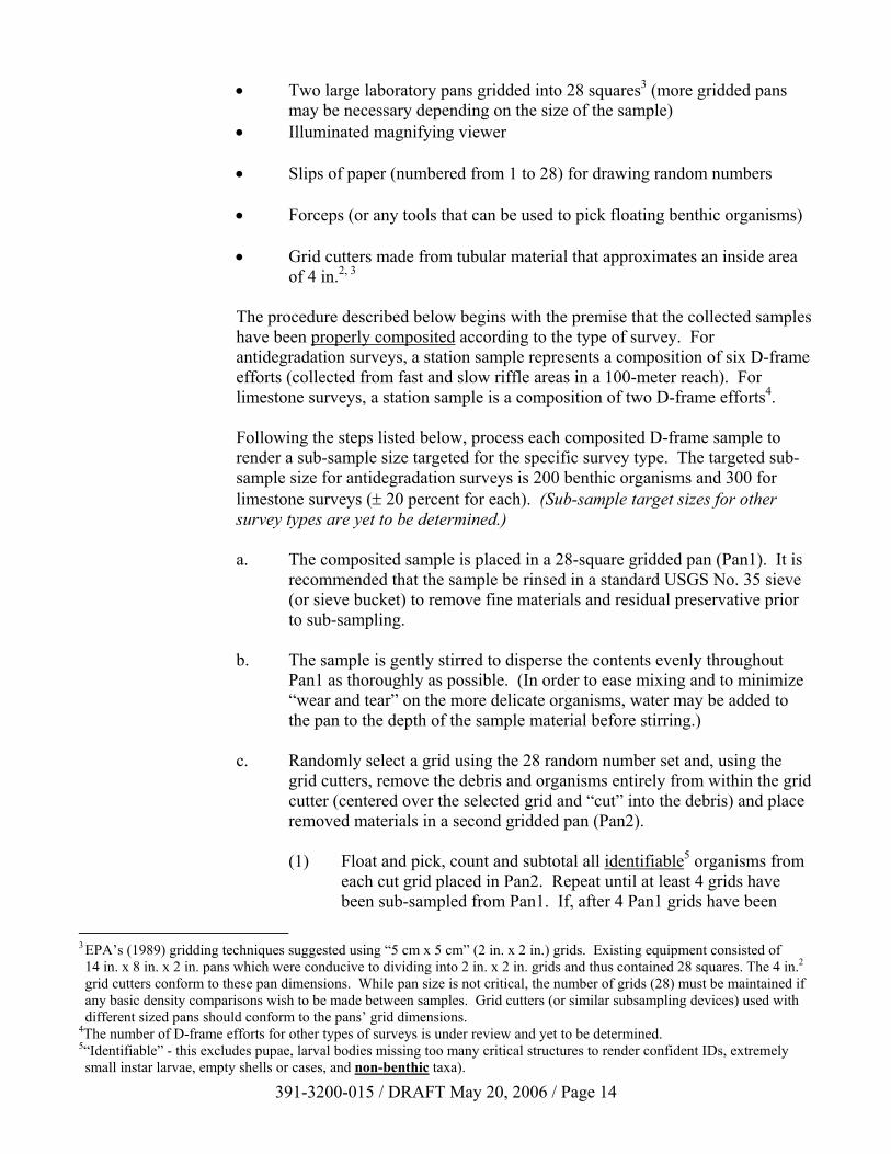
• Two large laboratory pans gridded into 28 squares3 (more gridded pans may be necessary depending on the size of the sample)

• Illuminated magnifying viewer • Slips of paper (numbered from 1 to 28) for drawing random numbers • Forceps (or any tools that can be used to pick floating benthic organisms) • Grid cutters made from tubular material that approximates an inside area

of 4 in.2, 3 The procedure described below begins with the premise that the collected samples

have been properly composited according to the type of survey. For antidegradation surveys, a station sample represents a composition of six D-frame efforts (collected from fast and slow riffle areas in a 100-meter reach). For limestone surveys, a station sample is a composition of two D-frame efforts4.

Following the steps listed below, process each composited D-frame sample to

render a sub-sample size targeted for the specific survey type. The targeted sub-sample size for antidegradation surveys is 200 benthic organisms and 300 for limestone surveys (± 20 percent for each). (Sub-sample target sizes for other survey types are yet to be determined.)

a. The composited sample is placed in a 28-square gridded pan (Pan1). It is

recommended that the sample be rinsed in a standard USGS No. 35 sieve (or sieve bucket) to remove fine materials and residual preservative prior to sub-sampling.

b. The sample is gently stirred to disperse the contents evenly throughout

Pan1 as thoroughly as possible. (In order to ease mixing and to minimize “wear and tear” on the more delicate organisms, water may be added to the pan to the depth of the sample material before stirring.)

c. Randomly select a grid using the 28 random number set and, using the

grid cutters, remove the debris and organisms entirely from within the grid cutter (centered over the selected grid and “cut” into the debris) and place removed materials in a second gridded pan (Pan2).

(1) Float and pick, count and subtotal all identifiable5 organisms from

each cut grid placed in Pan2. Repeat until at least 4 grids have been sub-sampled from Pan1. If, after 4 Pan1 grids have been

3 EPA’s (1989) gridding techniques suggested using “5 cm x 5 cm” (2 in. x 2 in.) grids. Existing equipment consisted of 14 in. x 8 in. x 2 in. pans which were conducive to dividing into 2 in. x 2 in. grids and thus contained 28 squares. The 4 in.2 grid cutters conform to these pan dimensions. While pan size is not critical, the number of grids (28) must be maintained if any basic density comparisons wish to be made between samples. Grid cutters (or similar subsampling devices) used with different sized pans should conform to the pans’ grid dimensions. 4The number of D-frame efforts for other types of surveys is under review and yet to be determined. 5“Identifiable” - this excludes pupae, larval bodies missing too many critical structures to render confident IDs, extremely small instar larvae, empty shells or cases, and non-benthic taxa).

391-3200-015 / DRAFT May 20, 2006 / Page 14

sorted, the subtotal is less than the targeted sub-sample (200 ± 20 percent), then continue to remove and sort grids one at a time until 200 organisms (± 20 percent) are obtained from Pan2. If the benthic organism yield from the 4 Pan1 grids exceeds the 200 ± 20 percent target (240+), then proceed to Step ii.

(2) With all of the 240+ identifiable organisms remaining in Pan2,

randomly select one grid and “back count” (removing) all the organisms from that grid. Repeat one grid at a time until the bug count remaining in Pan2 satisfies the “200 ± 20 percent” rule.

d. If not identified immediately, the sub-sample should be preserved and

properly labeled for future identification. e. The benthic material remaining (Pan1) after the target sub-sample has

been picked can be returned to its original sample jar and preserved. They shall be retained in accordance with quality assurance (QA) retention times as specified for this respective survey type.

f. Any grid chosen must be picked in its entirety. g. Record the final grid counts selected for each gridding phase (Pan1, Pan2

and Pan2 “back counting” as necessary) on the lab bench ID sheet for the sample.

Processing larger, excessive amounts of D-frame sample debris Hopefully, the collector will rarely have very large amounts of D-frame

materials to process. The reduction of large materials by careful removal, inspection and rinsing in a bucket or using a sieve prior to field preservation or at the lab is encouraged. However, if the amount of material composited in the field jars exceeds the functional sorting capacity of Pan1, then follow this guidance:

• Evenly distribute the material between as many pans as necessary • From each pan (Pan1a, Pan1b, etc.), remove debris and organisms

from 4 random grids and place in Pan2 as described in Step C.2.c. above

• Once the required 4 grids from each Pan1 have been placed in

Pan2, evenly and gently redistribute the materials as in Step C.2.b. • Then, resume processing, again as described in Step C.2.c.,

selecting a grid from Pan2 and placing the materials into a gridded Pan3

391-3200-015 / DRAFT May 20, 2006 / Page 15

• Process this material and repeat as described in Step C.2.c.i. until the targeted 200 ± 20 percent sub-sample is obtained from Pan3

• If, after processing 4 grids, the +20 percent upper limit (240+) is

obtained, follow “back counting” method in Step C.2.c.ii. • Once the targeted sub-sample is reached, continue with Step C.2.d. D. Quantitative Methods The type of sampling gear used is dependent on survey type and site-specific conditions.

The recommended gear includes Surber-type samplers (with 800-900µ mesh), artificial substrate (multi-plate) samplers (meeting specifications in Section IV.D.2) and grab-sample devices. The type of gear, dimensions and mesh size must be reported for all collections. When more than one gear type is used, the results must be recorded separately.

In order to limit the complications arising from compounding variables, follow the

guidelines discussed in Section II when selecting background stations or reference waterbodies and impact stations. Physical variables should be matched as closely as possible between the background and impact stations when selecting locations for placement of the sampling gear within each station. This helps minimize or eliminate the effects of compounding variables. An additional consideration is locating the samplers in areas where current, depth and substrate are optimal for gear efficiency. If the gear is used under sub-optimal conditions (i.e., slow current, bedrock, etc.), it should be clearly noted on field forms.

Macrobenthos often exhibit clustered distributions, and if the sample points are selected

within close proximity, only a single clustered population sample may be obtained rather than a generalized measure of the overall population within the selected sub-habitat. Spacing the sampling gear as far apart as possible within the sub-habitat can minimize the problem of clustered distributions.

1. Surber-Type Samplers. Surber-type samplers are defined as samplers that

delineate or confine an area of the stream bottom (usually 1 ft2), which is to be sampled by disturbing the enclosed substrate. The dislodged materials (organisms, detritus, other debris) are swept into an attached, tapering net. These samplers include the Surber Sampler, Portable Invertebrate Box Sampler (PIBS) and Hess Sampler. The sampling procedure for all these samplers and other similar devices are as follows:

a. The substrate will be completely disturbed within the confines of the

sampler frame to a depth of 3-4 in. (approximately 10 cm). Larger rocks should be gently but thoroughly “scrubbed” while being held in the net mouth.

b. Collect a minimum of 3 quantitative samples at each site. Do not

composite samples, but place each collection in a separate container.

391-3200-015 / DRAFT May 20, 2006 / Page 16

c. These quantitative samples may be processed in the manner described in Section IV.C.2, except that once all organisms have been floated and picked from the debris, it is not necessary to pick the “100+” sub-sample from a gridded pan. Evaluations using organisms collected by these quantitative methods rely on the total number of individuals from the entire sample.

d. The organisms may be identified to the taxonomic level deemed necessary

by the collector and problem being investigated. Samples may be split to expedite processing. Procedures for sub-sampling are defined in Elliott (1977) and in EPA (1990). In addition, a plankton splitter may be employed to sub-sample large numbers of chironomid larvae or other abundant taxa.

e. Complete a coded field form to ensure that the associated physical data is

recorded. 2. Multi-plate Samplers. Multi-plate artificial substrate samplers may be used

where water depth and/or substrate prevents the use of other sampling techniques. A description of the sampler used, including the type of artificial substrate, the individual component dimensions and total surface area, must be reported with each collection. In continuing investigations, the samplers must be uniform from year to year.

Physical variables should be matched as closely as possible when using the

samplers on an annual basis at the same location and between stations for cause/effect surveys. Matching these variables helps minimize or eliminate the compounding of variables. An additional consideration is locating the samplers in areas where the current, depth and substrate are optimal for gear efficiency while minimizing problems of theft and disturbance.

Multi-plate samples for WQN stations must conform to the following procedures: a. Place a minimum of 2 samplers at each site to help ensure the retrieval of

at least 1. b. Leave the samplers in place for a minimum of 6 weeks. The amount of

time the samplers are in place must be reported with each collection. c. Samplers should be enclosed in a net or plastic bag before retrieval to

prevent loss of organisms. When the use of nets or bags is not possible, retrieve the sampler with a smooth but rapid motion to minimize loss of organisms. The retrieved sampler should be immediately placed in a tray, scraped and all the scrapings preserved. Do not composite the samples. Preserve each separately.

d. The taxa should be identified to genus whenever possible. Samples may

be split to expedite processing. Procedures for sub-sampling are defined in Elliott (1977) or EPA (1973).

391-3200-015 / DRAFT May 20, 2006 / Page 17

e. Complete a coded field form to ensure that the associated physical data is recorded.

3. Grab Samplers. Where standard shallow-water sampling methodology is not

feasible, grab-sampling devices may be necessary. These include Ekman, Peterson or Ponar-style grab samplers. They are designed for use in deeper waters or in areas that have soft, unconsolidated substrate. These samplers are somewhat cumbersome and labor intensive to use. They are heavy, by design, so that they can be dropped from a boat and penetrate the substrate. They often need a boom and pulley retrieval system. For specific discussions on the advantages, disadvantages and sampling methodology, refer to EPA (1990).

E. Identification 1. Taxonomic Level. The level of identification for most aquatic

macroinvertebrates6 will be to genus based on the recommended references listed in Section IX. Some individuals collected will be immature and not exhibit the characteristics necessary for confident identification. Therefore, the lowest level of taxonomy attainable will be sufficient. Certain groups, however, may be identified to a higher taxonomic level as follows:

Snails (Gastropoda) - Family Clams, mussels (Bivalvia) - Family Flatworms (Turbellaria) identifiable planarids - genus or Family Planaridae others - Phylum Turbellaria Segmented worms (Annelida) aquatic earthworms & tubificids - Class Oligochaeta leaches - Class Hirudinea Moss animacules - Phylum Bryozoa Proboscis worms - Phylum Nemertea Roundworms - Phylum Nematoda Water mites- “Hydracarina” (an artificial taxonomic grouping of several mite

superfamilies) 2. Verifications. For QA purposes, certain laboratory invertebrate processing

procedures should be checked routinely. Normally, a colleague may perform these spot checks. These include the floating/picking steps, taxonomic identifications and total taxa list scans:

a. Sorting. After the floating and picking has been completed for samples

that require this treatment (PADEP-RBP, Surber-type, multi-plate and grab samples), the residue should be briefly scanned before discarding to

6 Presently, the identification of Chironomidae, or midges, is to the family level. Record macroinvertebrate identifications on forms similar to the Macroinvertebrate Enumeration form (3800-FM-WSFR0403) available on DEP’s website.

391-3200-015 / DRAFT May 20, 2006 / Page 18

ensure that the sample has been sufficiently picked. This should be done for 10 percent of the samples (or at least 1 sample) per survey.

b. Identification. For samples not involving litigation or enforcement issues,

laboratory bench ID sheets for all samples should be reviewed. Any unusual taxa or taxa that are not typical to the type of stream or water quality condition that was surveyed, should be checked. For samples involving legal issues, representative specimens of each taxon may need to be verified by independent expert taxonomists.

3. Sample Retention. For QA purposes, identified benthic macroinvertebrate

samples should be preserved and retained for later verifications. Based on the nature and purpose of the survey, retention times would vary:

a. Cause/effect surveys: until all legal issues have been resolved. b. Monitoring surveys: (1) WQN - 2 years (2) Reference WQN - 5 years c. Stream redesignation and use-attainability surveys: until after any

proposed stream classification changes become final (approximately 2 years).

d. Enforcement/compliance surveys: until all legal issues, including appeals

and related litigation, have been resolved.

391-3200-015 / DRAFT May 20, 2006 / Page 19

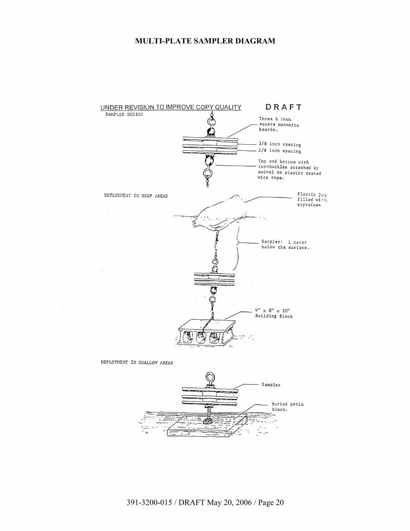
MULTI-PLATE SAMPLER DIAGRAM

391-3200-015 / DRAFT May 20, 2006 / Page 20

VI. FISHES An important aspect of determining the quality of surface waters and the degree of support of

designated uses is an assessment of the fish community. While not routinely sampled during every aquatic biology investigation, information on fish occurrence can be helpful in determining water quality and is essential when assessing use attainability.

There are several fish collection methods commonly used depending on survey purposes. These

include netting (gill, hoop and seine nets, for example), hook-and-line (angling and trot-lines) and electrofishing (backpack, tow boat and boat) methods. Of all the accepted fish collection methods available, electrofishing has proven to be the single most effective and popular method for fish sampling in streams. It is the most common fish collection method used by DEP and is discussed below. The remaining sampling methods will be discussed in the context of their recommended applications.

A. Electrofishing Considerations DEP “recognizes that electrofishing is an inherently hazardous activity for which safety is

a primary concern. The voltage and currents used are more than sufficient to cause serious injury or death to the collector. The environmental conditions under which these operations are conducted further increase the risks.” (Attachment A - Policy for Electrofishing Personnel and Equipment Safety in Appendix B). Due to these important concerns for electrofishing safety, all field team members must be trained in electrofishing techniques, safety precautions and equipment manufacturer’s operating procedures. It is the responsibility of the lead biologist (or crew chief) to verify that the crewmembers have this training. The first step in training a crewmember is to review the requirements presented in Appendix B (Introduction to Basic Electrofishing Techniques).

The safety of all personnel and the quality of the data are ensured through the adequate

education, training and experience of all members of the fish collection team. At least one (1) biologist with training, experience and certification in the principles and techniques of electrofishing must be involved in each sampling event.

1. Electrofishing Gear. Electrofishing methods rely on one of three main types of

gear platforms: backpacks, towboats or standard boats equipped with generators and hand-held or fixed probes. Collection gear consists of a wide variety of net sizes, shapes and configuration. Each team member must be insulated from the water and the electrodes; therefore, chest waders are required, and rubber gloves are recommended. Electrode and dip net handles must be constructed of insulating materials (fiberglass or wood). Electrofishing units must be equipped with functional safety switches. Field team members must not reach into the water unless the electrodes have been removed from the water or the electrofishing unit has been disengaged. These specific safety issues, along with electrofishing techniques, are presented in greater detail in Appendix B.1.

391-3200-015 / DRAFT May 20, 2006 / Page 21

B. Qualitative Fish Collection Methods The simplest form of fishery data is qualitative (presence/absence) and is generally easy

to obtain. A number of fish collection techniques, both active and passive, are available and should be selected for their efficiency in capturing a targeted species.

1. Small (Wadeable) Stream Methods. Generally, the length of stream sampled

should be 100 meters and the section chosen should contain the different habitats characteristic of the stream being studied. All habitat types should be sampled. The length of stream sampled may be increased if needed to obtain a representative sample. In cause/effect surveys, a reference station should be established for comparison to the impaired or affected site(s) (see macroinvertebrate methods).

a. Seines - Select a suitable area, which is generally a section having a

relatively smooth bottom. Beginning at the downstream end of the section, pull the seine upstream into the current as rapidly as possible, Ensuring that the bottom of the seine is in contact with the stream bottom. At the upstream end of the section, quickly bring the seine to the bank and lift it from the water, forming a “pocket” in its center. Remove all fish specimens for processing.

b. Electrofishing - For obtaining qualitative fish samples from most

wadeable streams, electrofishing with a backpack unit is the preferred method. However, if the targeted waters are wider wadeable streams or rivers, then the use of a towboat would be more appropriate. Electrofishing should proceed in an upstream direction, terminating at a physical barrier, if possible. In instances where a physical barrier is not present, block nets should be used. An attempt should be made to capture all fish in the electrical field.

c. Angling - In some instances, stream morphology or other factors may

preclude the use of many sampling methods. In such cases, angling may collect fish. Generally speaking, this method is inadequate to obtain population data because it is highly selective in the size and species of fish captured and the catch-per-unit effort is low. It can be used, however, as a supportive technique to verify the presence of sport fish or to obtain a limited number of fish for tissue analysis.

2. Large River, Lake and Pond Methods a. Electrofishing - A boat-mounted electrofisher can be used to obtain

limited fish abundance information or fish tissue samples in the littoral zone of large rivers and impounded waterbodies. A complete inventory cannot usually be obtained using this method of capture in these habitats because resulting population estimate is usually not practicable or accurate with any degree of confidence. Catch-per-unit effort information (e.g., number caught/hour, number caught/length of shoreline) may be used as a measure of abundance for comparisons between sites.

391-3200-015 / DRAFT May 20, 2006 / Page 22

b. Gill Nets - Gill nets may be used in slow-flowing rivers, lakes and ponds. Gill nets hang vertically and depend on fish moving into them. They should be set at right angles from the shoreline. For best results, the nets should be left overnight.

c. Hoop Nets - Hoop nets can be used in rivers and other waters where fish

movement is fairly predictable. These nets also depend on fish moving into them, and baiting the nets can sometimes enhance success.

d. Angling - While hook and line is not a good method for obtaining

population information, as noted above, it can be used to supplement the foregoing techniques or to obtain a limited number of specimens for tissue analysis.

e. Trot Line - Quite often, the best method for obtaining a sample of channel

catfish for tissue analysis is the use of a multiple-hook trot line left in place overnight. Note: Snapping turtles may also be collected by this method. If turtles are not the target organisms, place them on the bank away from high traffic area until they revive. Caution must be exercised before considering keeping them in the boat until they revive. Turtles that appear to be dead are often in a state of torpor following prolonged submergence, and may recover if left out of the water.

3. Fish Identification. To the extent possible, fish should be identified to species as

quickly as possible and released. Fish that cannot be identified in the field should be preserved in 10 percent formalin for later identification. A list of references for fish identification is found in Section IX.

4. Recordkeeping. Information on the length and width of stream sampled, species

collected, and all associated physical data must be recorded on a properly coded field form.

C. Quantitative Fish Collection Methods for Population Estimations When an estimate of fish populations (usually game fish) is needed, one of two

procedures employed by the PFBC will be used: 1) the Petersen or Mark-Recapture Method, or 2) the Zippin or Removal Method. The statistically based population estimates provided by these two methods are dependent on basic assumptions and prescribed sampling protocols that are discussed below. Generally, these methods will be used in streams small enough to easily electrofish. In extreme cases, a quantitative population count could be obtained through the addition of rotenone. This method should be considered a last resort and requires PFBC approval.

Sampling stations may be selected randomly or chosen to be representative of the length

of channel for which a population estimate is desired. In the latter case, 10 percent of the channel length under investigation should be sampled. In any case, the reach sampled should contain the different habitat types representative of the stream being studied. In addition to the fish data, all pertinent field data must be recorded on a coded field form.

391-3200-015 / DRAFT May 20, 2006 / Page 23

1. The Petersen or Mark-Recapture Method: The mark-recapture method is generally preferred over depletion or removal

methods and has been shown to be essentially unbiased when more than 50 percent of the population is marked.

a. Basic Assumptions: • The ratio of marked fish recovered to the total catch of the

recapture pass equals the ratio of the total number of fish marked and released to the total population.

• During the period between release and recapture, marked fish

suffer no greater mortality and emigrate no further than unmarked fish.

• No marks are lost, nor are any recaptured (marked) fish

overlooked. • Marked fish are caught at the same rate as unmarked fish and are

equally vulnerable to capture. • There are no additions to the population between passes. • Marked fish are randomly distributed throughout the sample area. b. Crew considerations. A typical crew on a small- to medium-size stream

having substantial game fish populations would consist of four persons. Two individuals will be electrofishing while a third person wearing the belly net (a combination holding net/measuring board suspended from a neck harness) will measure and mark fish on the marking run. The fourth person will record data and aid the electrofishing crew. With smaller populations of fish, the duties of the fourth person can often be absorbed by the individual marking and measuring fish. To avoid introducing possible sampling bias, crewmembers should retain their respective duties during both mark and recapture runs. It is especially important for the crewmember that marked the fish to be the one examining recaptured fish for his or her marks.

c. Field Procedure. Downstream and upstream limits of the sample section

should be chosen to minimize the emigration of fish out of the section. An upstream barrier such as a steep shallow riffle makes a good upstream end point. Any fish captured in the tail of the pool should be held and released in the head of the pool. Starting points should not be located in a fast riffle since initially marked fish may be displaced downstream. The tail of a workable pool makes a good starting spot. It is highly recommended that blocking nets be used, especially at the downstream limit of the section. Note: It is strongly recommended that the recapture pass be conducted the day following the marking pass. Conducting both mark and

391-3200-015 / DRAFT May 20, 2006 / Page 24

recapture runs on the same day should be avoided since marked fish may not have adequately recovered and become properly remixed with the remaining unmarked population, thereby violating a basic assumption of the mark-recapture method. If circumstances dictate that single-day sampling is necessary, consider the removal method instead (see Section C.2.).

In the marking pass, emphasis should be placed on marking as many fish

as possible. If the estimate is to cover all sizes of fish, then the various habitats present in the same section should be electrofished. While it is not practical (or necessary) to capture every individual, thorough coverage of the section in each pass will ensure that a high proportion of fish are marked and recaptured. Captured fish in the marking run will be measured (total length) to the nearest mm and given a caudal fin clip. As a suggestion, the removal of the dorsal lobe of the caudal fin provides an easily recognizable mark for trout species. Marked fish should be returned to the water as soon as possible, and efforts should be made to place the fish in quiet waters outside of the electrical field, rather than swift current that might displace them out of the section before recovery occurs. The lengths are recorded by species and in 10 mm increment size groups.

The recapture pass should encompass the same stream reach as was

sampled during the marking run. Fish captured should be placed in live bags, live wells or other well aerated containers. Captured fish are examined for the fin clip (recorded as either marked or unmarked), measured, and 10 fish from each 10 mm length group are weighed to the nearest gram. Data from both the marking and recapture efforts is recorded on the Mark-Recapture Field Data Sheet form (3800-FM-WSFR0107) available on DEP’s Web site.

d. Calculation Procedure. See Appendix A.1. for calculation procedures. 2. The Zippin or Removal Method: The removal method is recommended for use in small streams and where the

population is small (<2,000). This method is more appropriate than mark-recapture methods when single-day sampling is desired or there is concern that a substantial amount of immigration or emigration is likely to occur.

a. Basic Assumptions: • The rate of capture will decrease as the population increases. • >30 percent of the population is captured during each pass. • A closed population, i.e., there should be no movement of fish into

or out of the sample section.

391-3200-015 / DRAFT May 20, 2006 / Page 25

• The probability of capture during the removal is the same for each fish exposed to capture.

• The probability of capture remains constant from sampling to

sampling (in the same section) and sampling conditions and effort remain the same.

b. Crew Considerations. With the exception of the marking activities, crew

considerations would be similar to that of the mark-recapture method. c. Field Procedure. The complete survey should be conducted in 1 day.

Following selection of the stream reach to be sampled, blocking devices (seines or nets) are placed with particular care given to securing the bottom along the streambed and elevating the top several inches above the water. The entire section must be thoroughly electrofished with special emphasis given to preventing fish from evading capture. Consequently, larger streams may not lend themselves to this method, especially if only one electrofishing crew is available. Relatively large proportions of the population must be captured in order to obtain precise population estimates.

During and following each pass (removal), captured fish are placed in

separate holding facilities designated for each pass. Additional passes are then made in the same manner. This method of estimation can be conducted with as few as two passes; however, three have proven much more satisfactory and as many as four have been recommended. If additional help is available, fish can be processed while the crew conducts other passes. Data must be kept separate for each pass. Total lengths are recorded to the nearest mm and 10 weights are taken for each 10 mm group for each species per station.

d. Calculation Procedure. See Appendix A.2. for calculation procedures. 3. Index of Biotic Integrity (IBI) Assessment Collection Protocol: Aquatic life use assessments for most of the state’s wadeable streams have

traditionally relied on benthic macroinvertebrate protocols. These are usually cooler, higher gradient 1-3rd order streams. However, these benthic community methods are less well suited for larger, warm water streams. Pennsylvania’s fish-based Index of Biotic Integrity (IBI) Assessment protocol may be more applicable for these stream types.

a. Basic Assumptions. A Fish IBI protocol is a valuable stream assessment

tool, especially when applied to larger warm water streams, and can compliment existing benthic macroinvertebrate protocols used to assess the quality of Pennsylvania’s aquatic resources. It is labor intensive and relies on a one-pass electrofishing effort to capture and identify as many

391-3200-015 / DRAFT May 20, 2006 / Page 26

fish as possible. A suite of traditional fish community metrics is calculated to derive a single IBI score.

b. Standard Gear. Equipment considerations are comparable to those

discussed above in Sections A.1, A.2 and Appendix G.3. However, since IBI surveys may involve many personnel and cover a wide range of warm water habitat types, equipment needs can vary and are discussed in further detail below:

Nets designed for fish capture include a variety of types. Some are

designed to capture and hold larger fish and others designed to scoop small benthic-dwelling fish from among rocks. Both net types should be available for use and should have handles made of non-metallic materials and designed to adequately insulate persons from electric shock. Use 3-5 gallon capacity plastic buckets with plastic grips to avoid shock from the electrical field. Plastic holding tanks/containers designed to hold several buckets of water and fish shall be placed at streamside and/or be secured or mounted on tow barges or boats.

c. Safety Gear. All members of the electrofishing crew shall wear chest

waders with felt soles or cleats. Each crewmember should also wear polarized glasses to reduce surface glare, thereby aiding their ability to safely negotiate the stream bottom and to see and net fish. Life vests shall be worn by all boat electrofishing crewmembers and are optional in all other electrofishing scenarios.

d. Electrofishing Gear. May include any number or combination of

backpack and tow barge electrofishing units, or one boat alone or in combination with any number of backpack and tow barge units. The appropriate equipment will be determined when field reconnaissance is conducted.

The goal of appropriate electrofishing gear selection is to determine the

proper configuration needed to electrofish all habitat types and both banks in a side-to-side sweeping motion. The combined use of multiple electrofishing units is necessary to create an effective electrical barrier to minimize fish escape. This is critical in quantitative electrofishing surveys. Additional electrofishing units may be needed where conductivity is low or when stream morphology limits the size or effectiveness of the electrical field (i.e. wide, low-flowing streams with abundant boulders that interrupt stream flow).

e. Field Reconnaissance And Reach Length. Field reconnaissance

includes selecting an appropriate reach to sample where access is adequate and the presence of a warm water fish community can be confirmed by sight or through qualitative electrofishing techniques, snorkeling, and/or input from local anglers. When electrofishing reconnaissance is needed, it shall be conducted no less than one week prior to when the quantitative

391-3200-015 / DRAFT May 20, 2006 / Page 27

electrofishing survey is conducted to allow the fish community adequate time to recover from the disturbance.

Warm water fish communities are typically dominated by shiners, chubs,

minnows, and stonerollers (Cypriniformes) and bass, sunfish, and darters (Perciformes). It is critical to verify the presence of a warm water fish community prior to sampling because it may greatly affect the outcome of IBI metric calculations, which were calibrated specifically to assess warm water communities. Additionally, many warm water species emigrate as stream temperatures fluctuate with the changing seasons.

During field reconnaissance, the appropriate reach length is determined

and marked off using a highly visible marker such as blaze-orange ribbon or surveyor’s flags. The starting point is first determined and marked on a USGS 7.5’ topographical quadrangle map. In the first 100 meters, 5 wetted channel widths are measured using a measuring tape (every 20 meters from the starting point) and averaged. Generally, reach length will be determined as 10 times the average wetted channel width. Reach length shall be a minimum of 100 meters and should not exceed 400 meters. Specifically, reach length may be extended if the appropriate length calculated falls in the middle of a habitat sequence or excludes a particular type of habitat.

f. Sampling Conditions. Sampling should be conducted from May through

October. This window may be adjusted in atypical precipitation years. Conditions at the time of sampling shall be low to normal summer flow with good water clarity for effective sampling. If stream conditions do not meet these criteria, sampling should be postponed.

g. Electrofishing. Electrofishing will consist of a one-pass effort performed

in a zigzag pattern that covers both banks and all available habitats through the entire length of a predetermined reach. Electrofishing will be conducted in an upstream direction. Starting and ending points should be selected to take advantage of natural barriers to fish escape such as riffle heads and tails of runs or cascades. Block nets may be used if natural barriers are inadequate or absent.

Fish are netted and placed in buckets or directly into a holding tank or live

well. When buckets become full, they are either exchanged for empty buckets or carried to a holding tank and carefully emptied. When the holding tank is full, it may be carefully replaced by any excess crewmembers or by an identification crew. Time spent at a site can be greatly reduced by having extra crew members solely responsible for exchanging holding tanks and getting a head start on identifying and enumerating fish while the electrofishing is in progress. These crewmembers must wear chest waders at all times.

The goal of quantitative electrofishing is to collect as many fish as

possible from all species regardless of size. Netters should be conscious

391-3200-015 / DRAFT May 20, 2006 / Page 28

of their own effort to be sure that game fish are not targeted. Specialized nets that allow benthic minnow species to be easily collected should be used in all electrofishing scenarios.

h. Electrofishing Crew Roles and Responsibilities. Electrofishing crew

roles and responsibilities for IBI surveys are discussed below and should be reviewed each day as required in Appendix G - Electrofishing Techniques, Section 4.

The Primary Crew or Project Leader assigns roles and responsibilities

to each crew member and directs the entire sampling effort. This person is responsible for assuring that fish are collected in a consistent and safe manor and is also responsible for managing the electrical field throughout sampling. The Primary Crew Leader is ultimately responsible for collecting and organizing all field forms and enumeration records.

Probers are responsible for applying the electrical field, maintaining a

constant field while electrofishing, and turning off the electrical current during emergencies. They may choose to carry two electrical probes or one probe and one net.

Netters typically follow behind the Probers, either at a safe distance

directly behind or downstream on either side of a Prober. Bucket Handlers follow Probers and Netters at a safe distance, always

being aware of the movement of net handles and probes around them. They should carry their buckets with two hands at all times and “present” their buckets to Netters in such a way that allows them to quickly and safely empty their nets without spilling fish. This is done by holding the bucket by the handle with one hand while placing the other hand on the bottom of the bucket and tilting it forward to “present” the opening of the bucket to the Netters while pulling the handle down and out of the way of the opening.

Tow Barge Pullers and Boat Captains are solely responsible for pulling

or navigating their electrofishing unit through the reach, following the direction of the Probers or instructions given by the Primary Crew Leader.

Fish Identifiers - see below Data Recorders - see below i. Fish Identification. All fish captured should be identified to species at

streamside, and enumerated using the common name of the species to simplify data recording. All fish that can be practically identified at streamside should be released as they are enumerated. Any specimens that cannot be identified to species with absolute certainty, should be preserved in 10 percent buffered formalin (or alternatively 50 percent isopropanol) solution, and taken back to the laboratory for bench-top identification.

391-3200-015 / DRAFT May 20, 2006 / Page 29

Endangered, threatened, or candidate species should be identified, enumerated, and released immediately on site. Fish Identifiers should familiarize themselves with all species of special concern to avoid misidentifying or preserving these species.

j. Enumeration and Record Keeping. As per quality assurance guidelines,

Data recorders should dictate the pace of Fish Identifiers so that accurate enumeration records can be kept. In scenarios where there is more than one Data Recorder, they should be spaced far enough apart to avoid confusion when Fish Identifiers are calling out species names. The number of Fish Identifiers per Data Recorder should also be kept at a minimum to avoid confusion.

Fish data enumerations should be recorded on standardized waterproof

field forms in waterproof ink or pencil. After all fish have been enumerated and released or preserved, these forms should be given to the Primary Crew Leader.

k. IBI Metrics Calculation. (Under development - IBI metrics and scoring

procedures are under development for use for IBI assessments.) D. Fish Tissue Sampling Methods Samples for determination of fish tissue contaminants may be collected as part of the

WQN, during special studies, or in response to an environmental emergency. When needed, the following procedures should be employed to obtain fish tissue samples:

1. Collect fish (electrofishing, seine, gill net, rotenone, angling, other) taking care

not to contaminate specimens with gasoline, motor oil, sediment or soil. Record method used on the Field Data Sheet Tissue Sampling form (3800-FM-WSFR0060) available on DEP’s Web site.

2. Measure the total length of each specimen in the sample to the nearest tenth of an

inch. Weigh each specimen in the sample to the nearest ounce (or tenth of an ounce). Record both on the Field Data Sheet Tissue Sampling form.

3. Note external appearance and general condition - i.e., tumors, lesions, etc. on the

Field Data Sheet Tissue Sampling form. 4. Prepare sample: a. Whole Fish - Wrap composite sample (or individual fish if necessary for

specific study) in clean, commercial (restaurant) grade aluminum foil allowing only the dull foil surface to contact fish tissue. Indicate sample type on the Field Data Sheet Tissue Sampling form.

391-3200-015 / DRAFT May 20, 2006 / Page 30

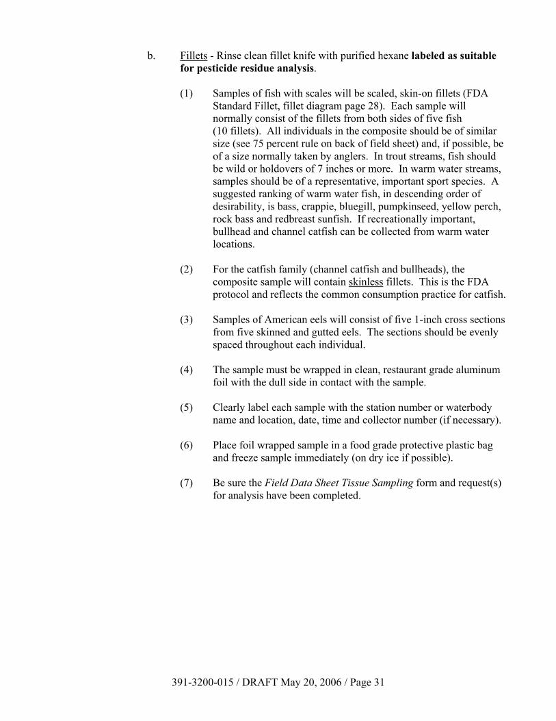
b. Fillets - Rinse clean fillet knife with purified hexane labeled as suitable for pesticide residue analysis.

(1) Samples of fish with scales will be scaled, skin-on fillets (FDA

Standard Fillet, fillet diagram page 28). Each sample will normally consist of the fillets from both sides of five fish (10 fillets). All individuals in the composite should be of similar size (see 75 percent rule on back of field sheet) and, if possible, be of a size normally taken by anglers. In trout streams, fish should be wild or holdovers of 7 inches or more. In warm water streams, samples should be of a representative, important sport species. A suggested ranking of warm water fish, in descending order of desirability, is bass, crappie, bluegill, pumpkinseed, yellow perch, rock bass and redbreast sunfish. If recreationally important, bullhead and channel catfish can be collected from warm water locations.

(2) For the catfish family (channel catfish and bullheads), the

composite sample will contain skinless fillets. This is the FDA protocol and reflects the common consumption practice for catfish.

(3) Samples of American eels will consist of five 1-inch cross sections

from five skinned and gutted eels. The sections should be evenly spaced throughout each individual.

(4) The sample must be wrapped in clean, restaurant grade aluminum

foil with the dull side in contact with the sample. (5) Clearly label each sample with the station number or waterbody

name and location, date, time and collector number (if necessary). (6) Place foil wrapped sample in a food grade protective plastic bag

and freeze sample immediately (on dry ice if possible). (7) Be sure the Field Data Sheet Tissue Sampling form and request(s)

for analysis have been completed.

391-3200-015 / DRAFT May 20, 2006 / Page 31

391-3200-015 / DRAFT May 20, 2006 / Page 32

VII. OTHER BIOLOGICAL-BASED SAMPLING METHODS A. Lake Specific Methods 1. Plankton Sampling Method (Modified Standard Method 1002a) This plankton sampling method was developed for use during Water Quality

Network sampling, but can be used for any qualitative plankton sampling. a. Anchor boat over sampling location and record field observations. Station No. DO profile (Hydrolab) Date Temperature profile (Hydrolab) Time Meteorological conditions Water depth Air temperature Water transparency Estimated Wind speed/direction (Secchi Disk) Percent cloud cover b. Execute two vertical plankton tows with a simple conical or Wisconsin

style net rigged with No. 20 (76 micron) nylon mesh. Each tow should be initiated at lake bottom and traverse the entire water column at a rate of approximately 0.5 meters/second (hand retrieval speed).

c. Organisms collected are washed into the sample container after each

tow. Both tows are composited into one sample preserved with Lugol’s solution applied at the rate of 0.3 milliliters per 100 milliliters of sample.

d. Properly label sample and forward to the Bureau of Laboratories in

Harrisburg via courier service. The sample should be accompanied by a completed ERBL-151 - “Bacteriological Analyses” form with the note “Qualitative Plankton Sample” entered into the comment block.

e. Field observations, including the temperature and DO profile, should

be forwarded to the Division of Water Quality Standards, BWSFR, within 30 days of sample collection.

f. To convert the sample to quantitative, calculate the volume of water

filtered during the two tows by multiplying (lake depth) x 2 x (area of plankton net opening) and enter the figure on the Lake Reservoir Field Data Sheet (3800-FM-WSFR0050) form.

391-3200-015 / DRAFT May 20, 2006 / Page 33

2. Chlorophyll-a Sampling Method This sampling method was developed for use during Water Quality Network

sampling, but can be used for any qualitative plankton sampling. a. Anchor boat over sampling location and record field observations. Station No. DO profile (Hydrolab) Date Temperature profile (Hydrolab) Time Meteorological conditions Water depth Air temperature Water transparency Estimated Wind speed/direction (Secchi Disk) Percent cloud cover b. Collect water sample with a Kemmerer or other remote sampling

device at a depth of 1 meter below the surface. c. Filter water through a 47 mm diameter glass filter. Record the volume

of water filtered. d. Place filter in a plastic petri dish, wrap in aluminum foil to shield from

light and freeze on dry ice. e. Properly label sample and forward to the Bureau of Laboratories in

Harrisburg via courier service. A completed ERBL-151 - “Bacteriological Analyses” form with the note “Chlorophyll-a Sample” entered into the comment block should accompany the sample.

f. Field observations, including the temperature and DO profile, should

be forwarded to the Division of Water Quality Standards, BWSFR, within 30 days of sample collection.

B. Bacteriological Sampling Method This method applies to all surface waters of the Commonwealth of Pennsylvania,

including streams, impounded waters, lakes, springs, and wetlands. The Department shall monitor fecal coliform bacterial densities as an indicator of

recreational use attainment. Fecal coliform bacteria are used as indicators of possible sewage contamination because they are commonly found in human and animal feces. Although fecal coliforms are generally not harmful themselves, they indicate the possible presence of pathogenic (disease causing) bacteria, viruses and protozoa that also live in human and animal digestive systems. Therefore, their presence in a waterbody suggests that pathogenic microorganisms may be present as well, and that water contact recreation such as swimming may be a health risk.

391-3200-015 / DRAFT May 20, 2006 / Page 34

1. Sampling Frequency and Duration a. Bacteriological sampling for determining water contact recreational

use attainment should be conducted during the swimming season (May 1 through September 30). At least two sampling groups must be collected per site to effectively characterize chronic conditions. A sampling group consists of 5 bacteriological samples collected on different days during a 30-day period and spanning a minimum of 14 days. It is best to sample at a different hour of the day for each of the five days to minimize the effect of timed releases from point source discharges.

b. Bacteriological sampling for determining potable water supply use

attainment should be conducted year-round. The use attainment status of these segments is defined by comparing the results of average total coliform densities calculated from sampling groups of at least two per month to the monthly average criterion outlined in Pennsylvania’s Water Quality Standards.

2. Sampling Design a. Targeted Sampling - Impaired waterbodies with the highest potential

to have high bacteriological levels shall be targeted first. Such impairment sources include municipal point sources, combined sewer overflows, and agricultural sources relating to manure application, livestock grazing, and animal feeding. Other targeted sites may be placed in areas of important recreational activities or where land use practices may contribute to potential bacteriological problems.

b. Probabilistic Sampling - A random probabilistic design shall be

employed for additional bacteriological monitoring. The purpose of the probabilistic sampling design is to determine the magnitude of the bacteriological problem within a watershed, stream class, or land use type. Probabilistic sampling design will be determined on a watershed scale to randomly select sites where bacteriological monitoring will occur. The design will focus on site selection and randomization calculated from target precisions and confidence levels.

Once a target number of sites are determined for a watershed based on

precision and confidence level, the randomized site selection process will occur. The site selection process will be weighted based on Strahler stream order and land use. The actual site selection process is done using a grid system overlaid on a GIS map of all streams in the sample population, or all streams that could potentially be monitored for bacteriological analysis. After the grid process is complete, the target number of sample sites are chosen at random.

391-3200-015 / DRAFT May 20, 2006 / Page 35

3. Equipment. Bacteriological samples shall be collected using bottles that have been pre-

sterilized and contain the proper amount of dechlorinating agent (preservative). DEP-supported sampling activities use 125-mL, screw-capped, polypropylene bottles with sodium thiosulfate added to neutralize the effects of residual chlorine.

4. Sample Collection Methodology. In general: Sample in the main current in the area of the greatest flow. Do

not sample the water’s edge and avoid stagnant water. a. After wading to the desired sampling location, pause to allow

disturbed sediment to wash downstream. Do not collect water that is clouded by the sediment you disturb.

b. Stand facing upstream. c. Remove the cap from a 125-mL BacT bottle. Avoid touching the

inside of the bottle or the cap. If you accidentally touch the inside of the bottle or cap, a new bottle must be used.

d. DO NOT RINSE THE BOTTLE! e. Sample water from a depth of 8 to 12 inches beneath the surface. If

the water is less than 16 inches deep, collect the sample at mid-depth. If the water is less than 4 inches deep, find a new place to sample where the water is deeper.

f. Grasp the uncapped bottle near its base with the opening pointing

downward and plunge it below the water surface. Turn the submerged bottle into the current and away from you. In slower current, push the bottle underneath the surface and away from you as if dipping water in an upstream direction.

g. DO NOT FILL THE BOTTLE COMPLETELY. Allow one-inch of

air space. The sample is shaken at the laboratory prior to analysis and the air space makes this easier.

h. Recap the bottle carefully, making sure not to touch the inside of the

bottle or lid and tighten. i. Dry the outside of the bottle and either place an adhesive label on the

bottle or write the sample information directly on the bottle in permanent marker.

j. Place each bottle inside a Ziploc plastic bag and seal it before putting

them in the cooler with ice. Place all Bacteriological Analyses forms

391-3200-015 / DRAFT May 20, 2006 / Page 36

in an additional plastic bag and place them inside the cooler on top of the ice.

k. Deliver samples to the laboratory within 30 hours of collection

accompanied by a completed ERBL-151 - “Bacteriological Analyses” form.

5. Quality Control. For every set of 5 samples, each collector shall complete one blank and one

duplicate sample. The blank sample will be used to test the laboratory’s accuracy while the duplicate sample will test the laboratory’s precision.

a. To complete a blank sample: Fill a 125-mL BacT bottle with sterile

(autoclaved) water from DEP’s laboratory. Label the bottle consistent with regular water samples, but be sure not to indicate on the bottle that the sample is a blank. Record the blank sample information on the same BIS-02 form as used for the regular water sample completed concurrently.

b. To complete a duplicate sample: Take a second 125-mL BacT bottle

with you into the stream. After filling the first bottle (the test sample), fill a second bottle (the duplicate sample) from the same location and depth using the same technique. Label the duplicate sample as you would the test sample, but do not indicate that the sample is a duplicate. Record the duplicate sample information on the same BIS-02 form as used for the regular water sample completed concurrently.

6. Laboratory Results. Fecal coliforms are reported by the laboratory as the number of colony

forming units per 100 milliliters (CFUs/100 mL). 7. Data Processing. A geometric mean shall be calculated for each sampling group (5 samples

collected on different days in a 30-day period). To calculate a geometric mean of 5 samples, first compute the logarithm of

each sample result and then calculate the average of the logarithm values. Finally, convert this product back to a normal value by computing the antilog of the product. The following examples illustrate how this is done:

391-3200-015 / DRAFT May 20, 2006 / Page 37

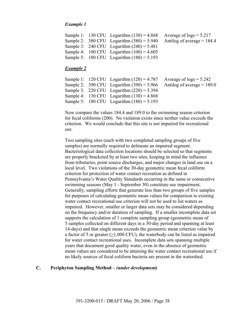
Example 1

Sample 1: 130 CFU Logarithm (130) = 4.868 Average of logs = 5.217 Sample 2: 380 CFU Logarithm (380) = 5.940 Antilog of average = 184.4 Sample 3: 240 CFU Logarithm (240) = 5.481 Sample 4: 100 CFU Logarithm (100) = 4.605 Sample 5: 180 CFU Logarithm (180) = 5.193

Example 2

Sample 1: 120 CFU Logarithm (120) = 4.787 Average of logs = 5.242 Sample 2: 390 CFU Logarithm (390) = 5.966 Antilog of average = 189.0 Sample 3: 220 CFU Logarithm (220) = 5.394 Sample 4: 130 CFU Logarithm (130) = 4.868 Sample 5: 180 CFU Logarithm (180) = 5.193

Now compare the values 184.4 and 189.0 to the swimming season criterion

for fecal coliforms (200). No violation exists since neither value exceeds the criterion. We would conclude that this site is not impaired for recreational use.

Two sampling sites (each with two completed sampling groups of five

samples) are normally required to delineate an impaired segment. Bacteriological data collection locations should be selected so that segments are properly bracketed by at least two sites, keeping in mind the influence from tributaries, point source discharges, and major changes in land use on a local level. Two violations of the 30-day geometric mean fecal coliform criterion for protection of water contact recreation as defined in Pennsylvania’s Water Quality Standards occurring in the same or consecutive swimming seasons (May 1 - September 30) constitute use impairment. Generally, sampling efforts that generate less than two groups of five samples for purposes of calculating geometric mean values for comparison to existing water contact recreational use criterion will not be used to list waters as impaired. However, smaller or larger data sets may be considered depending on the frequency and/or duration of sampling. If a smaller incomplete data set supports the calculation of 1 complete sampling group (geometric mean of 5 samples collected on different days in a 30-day period and spanning at least 14-days) and that single mean exceeds the geometric mean criterion value by a factor of 5 or greater (>1,000 CFU), the waterbody can be listed as impaired for water contact recreational uses. Incomplete data sets spanning multiple years that document good quality water, even in the absence of geometric mean values are considered to be attaining the water contact recreational use if no likely sources of fecal coliform bacteria are present in the watershed.

C. Periphyton Sampling Method – (under development)

391-3200-015 / DRAFT May 20, 2006 / Page 38

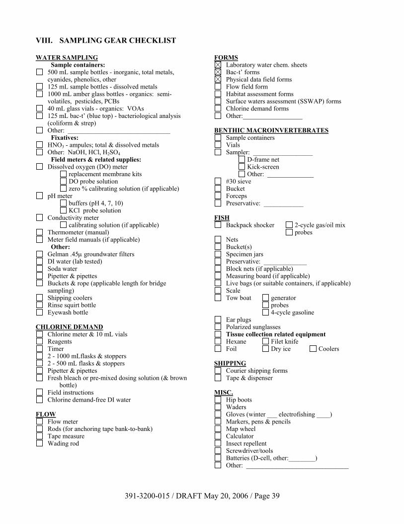
VIII. SAMPLING GEAR CHECKLIST WATER SAMPLING Sample containers:

500 mL sample bottles - inorganic, total metals, cyanides, phenolics, other

125 mL sample bottles - dissolved metals 1000 mL amber glass bottles - organics: semi-

volatiles, pesticides, PCBs 40 mL glass vials - organics: VOAs 125 mL bac-t’ (blue top) - bacteriological analysis

(coliform & strep) Other: _______________________________

Fixatives: HNO3 - ampules; total & dissolved metals Other: NaOH, HCl, H2SO4

Field meters & related supplies: Dissolved oxygen (DO) meter

replacement membrane kits DO probe solution zero % calibrating solution (if applicable)

pH meter buffers (pH 4, 7, 10) KCl probe solution

Conductivity meter calibrating solution (if applicable)

Thermometer (manual) Meter field manuals (if applicable)

Other: Gelman .45µ groundwater filters DI water (lab tested) Soda water Pipetter & pipettes Buckets & rope (applicable length for bridge

sampling) Shipping coolers Rinse squirt bottle Eyewash bottle

CHLORINE DEMAND

Chlorine meter & 10 mL vials Reagents Timer 2 - 1000 mLflasks & stoppers 2 - 500 mL flasks & stoppers Pipetter & pipettes Fresh bleach or pre-mixed dosing solution (& brown

bottle) Field instructions Chlorine demand-free DI water

FLOW

Flow meter Rods (for anchoring tape bank-to-bank) Tape measure Wading rod

FORMS Laboratory water chem. sheets Bac-t’ forms Physical data field forms Flow field form Habitat assessment forms Surface waters assessment (SSWAP) forms Chlorine demand forms Other:__________________

BENTHIC MACROINVERTEBRATES

Sample containers Vials Sampler: __________________

D-frame net Kick-screen Other: ______________

#30 sieve Bucket Forceps Preservative: ____________

FISH

Backpack shocker 2-cycle gas/oil mix probes

Nets Bucket(s) Specimen jars Preservative: _____________ Block nets (if applicable) Measuring board (if applicable) Live bags (or suitable containers, if applicable) Scale Tow boat generator

probes 4-cycle gasoline

Ear plugs Polarized sunglasses Tissue collection related equipment Hexane Filet knife Foil Dry ice Coolers

SHIPPING

Courier shipping forms Tape & dispenser

MISC.

Hip boots Waders Gloves (winter ___ electrofishing ____) Markers, pens & pencils Map wheel Calculator Insect repellent Screwdriver/tools Batteries (D-cell, other:________) Other: _______________________________

391-3200-015 / DRAFT May 20, 2006 / Page 39

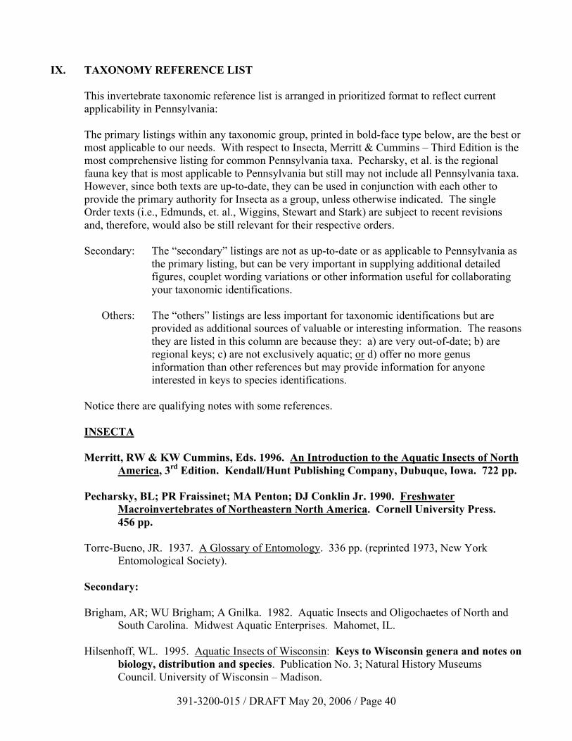
IX. TAXONOMY REFERENCE LIST This invertebrate taxonomic reference list is arranged in prioritized format to reflect current

applicability in Pennsylvania: The primary listings within any taxonomic group, printed in bold-face type below, are the best or

most applicable to our needs. With respect to Insecta, Merritt & Cummins – Third Edition is the most comprehensive listing for common Pennsylvania taxa. Pecharsky, et al. is the regional fauna key that is most applicable to Pennsylvania but still may not include all Pennsylvania taxa. However, since both texts are up-to-date, they can be used in conjunction with each other to provide the primary authority for Insecta as a group, unless otherwise indicated. The single Order texts (i.e., Edmunds, et. al., Wiggins, Stewart and Stark) are subject to recent revisions and, therefore, would also be still relevant for their respective orders.

Secondary: The “secondary” listings are not as up-to-date or as applicable to Pennsylvania as

the primary listing, but can be very important in supplying additional detailed figures, couplet wording variations or other information useful for collaborating your taxonomic identifications.

Others: The “others” listings are less important for taxonomic identifications but are

provided as additional sources of valuable or interesting information. The reasons they are listed in this column are because they: a) are very out-of-date; b) are regional keys; c) are not exclusively aquatic; or d) offer no more genus information than other references but may provide information for anyone interested in keys to species identifications.

Notice there are qualifying notes with some references. INSECTA Merritt, RW & KW Cummins, Eds. 1996. An Introduction to the Aquatic Insects of North

America, 3rd Edition. Kendall/Hunt Publishing Company, Dubuque, Iowa. 722 pp. Pecharsky, BL; PR Fraissinet; MA Penton; DJ Conklin Jr. 1990. Freshwater

Macroinvertebrates of Northeastern North America. Cornell University Press. 456 pp.

Torre-Bueno, JR. 1937. A Glossary of Entomology. 336 pp. (reprinted 1973, New York

Entomological Society). Secondary: Brigham, AR; WU Brigham; A Gnilka. 1982. Aquatic Insects and Oligochaetes of North and

South Carolina. Midwest Aquatic Enterprises. Mahomet, IL. Hilsenhoff, WL. 1995. Aquatic Insects of Wisconsin: Keys to Wisconsin genera and notes on

biology, distribution and species. Publication No. 3; Natural History Museums Council. University of Wisconsin – Madison.

391-3200-015 / DRAFT May 20, 2006 / Page 40

391-3200-015 / DRAFT May 20, 2006 / Page 41

Others: Usinger, RL, et al. 1956. Aquatic Insects of California with Keys to North American Genera

and California Species. Univ. of California Press, Berkely and Los Angeles. 508 pp. EPHEMEROPTERA Merritt & Cummins and Pescharsky, et al. Edmunds, GF, Jr.; SL Jensen; L Berner. 1976. The Mayflies of North and Central

America, University of Minnesota Press. 330 pp. Secondary: McCafferty, WP. 1975. The Burrowing Mayflies of the United States (Ephemeroptera:

Ephemeroidea). Trans. Amer. Ent. Soc. 101:447-504. Morihara, DK & WP McCafferty. 1979. The Baetis Larvae of North America (Ephemeroptera:

Baetidae). Trans. Amer. Ent. Soc. 105:139-221. Others: Burks, BD. 1953. The Mayflies, or Ephemeroptera, of Illinois. Bull. Ill. Nat. Hist. Surv.

26:1-216. (Reprinted 1975, Entomological Reprint Specialists.) Hucko, S & GR Finni. 1974. A Key to the Mayfly Nymphs (Insecta: Ephemeroptera) of

Pennsylvania and a Checklist of Pennsylvania Mayfly Species. Allegheny College Environmental Studies Report 19. 19 pp.

Needham, JG; JR Traver; VC Hsu. 1935. The Biology of Mayflies with a Systematic Account

of North American Species. Comstock, Ithaca. 759 pp. PLECOPTERA Stewart, KW & BP Stark. 2002. Nymphs of North American Stonefly Genera (Plecoptera)

2nd Edition. Thomas Say Foundation. Entomological Society of America. 12:1-509. Secondary: _____ & _____. 1984. Nymphs of North American Perlodinae Genera (Plecoptera:

Perlodidae). Great Basin Nat. 44:373-415. Surdick, RF. 1985. Nearctic Genera of Chloroperlinae (Plecoptera: Chloroperlidae). Illinois

Biological Monographs #54. University of Illinois Press. 146 pp.

Others: Surdick, RF & KC Kim. 1976. Stoneflies (Plecoptera of Pennsylvania): A Synopsis. Penn

State Univ. Agri. Exp. St. Bull. 808. 73 pp. (Caution - Some stonefly genera that have been collected in Pennsylvania are not included in this publication.)

Frison, TH. 1935. The Stoneflies, or Plecoptera, of Illinois. Bull Ill. Nat. Hist. Surv.

20:281-471. (Reprinted 1975, Entomological Reprint Specialists.) Hitchcock, SW. 1974. Guide to the Insects of Connecticut. Part VII. The Plecoptera or

Stoneflies of Connecticut. Bull. Conn. State Geol. Nat. Hist. Surv. 107:1-262. Harper, PP & HBN Hynes. 1971. The Nymphs of the Taeniopterygidae of Eastern Canada

(Insecta: Plecoptera). Can. J. Zool. 49:941-947. _____ & _____. 1971. The Leuctridae of Eastern Canada (Insecta: Plecoptera). Can. J. Zool.

49:915-920. _____ & _____. 1971. The Capniidae of Eastern Canada (Insecta: Plecoptera). Can. J. Zool.

49:921-940. _____ & _____. 1971. The Nymphs of the Nemouridae of Eastern Canada (Insecta:

Plecoptera). Can. J. Zool. 49:1129-1142. Kondratieff, BC; RF Kirchner; JR Voshell, Jr. 1981. Nymphs of Diploperla. Ann. Entomol.

Soc. Am. 74:428-30. TRICOPTERA Merritt & Cummins and Pescharsky, et al. Wiggins, GB. 1996. Larvae of the North American Caddisfly Genera (Tricoptera), 2nd

Edition. University of Toronto Press, Toronto. 457 pp. Others: Ross, HH. 1944. The Caddisflies or Tricoptera of Illinois. Bull. Ill. Nat. Hist. Surv. 23:1-326.

(Reprinted 1972, Entomological Reprint Specialists.) Hydropsychidae Schefter, PW & GB Wiggins. 1986. A Systematic Study of the Nearctic Larvae of the

Hydropsyche morosa Group (Trichoptera: Hydropsychidae). Royal Ontario Museum. 94 pp.

Others: Schuster, GA & Etnier, DA. 1978. A manual for the Identification of the Larvae of the

Caddisfly Genera Hydropsyche Pictet and Synphitopsyche Ulmer on Eastern and Central

391-3200-015 / DRAFT May 20, 2006 / Page 42

North America (Trichoptera: Hydropsychidae). Report No. EPA-600/4-78-060. USEPA, Cincinnati. 128 pp.

Rhyacophila species Weaver III, JS & JL Sykora. 1979. The Rhyacophila of Pennsylvania with Larval

Descriptions of R. banksi and R. carpenteri (Trichoptera: Rhyacophilidae). Annal. Carnegie Museum. 48:403-423. (Note: Flint (1962) must be used in conjunction with this paper since it relies on some of Flint’s figures for complete characteristics.)

Secondary: Flint, OS, Jr. 1962. Larvae of the Caddis Fly Genus Rhyacophila in Eastern North America

(Trichoptera: Rhyacophilidae). Proc. U.S. Nat. Mus. 113:465-493. DIPTERA Merritt & Cummins and Pescharsky, et al. Others: Johannsen, OA (Part V by Lillian C. Thomsen). Aquatic Diptera. (Reprinted 1969 from Memoirs

Nos. 164, 167, 205, 210 of Cornell University Agric. Exp. Station Entomological Reprint Specialists.) Chironomidae Merritt & Cummins and Pescharsky, et al. Although the following references are regional in nature, they provide photograph figures of key characters for

almost all the common genera found in Merritt & Cummins. Secondary: Oliver, DR & ME Roussel. 1983. The Insects and Arachnids of Canada. Part 11. The Genera

of Larval Midges of Canada. Diptera: Chironomidae. Agric. Can. Publ. 1746:1-263. Simpson, KW & RW Bode. 1980. Common Larvae of Chironomidae (Diptera) from New York

State Streams and Rivers, with Particular Reference to the Fauna of Artificial Substrates. Bull. N.Y. State Mus. 439:1-105.

Others: Mason, WT, Jr. 1973. An Introduction to the Identification of Chironomid Larvae. Nat.

Environ. Res. Cent./EPA. Cincinnati, OH. 90 pp. Note: This key was developed from specimens found in the larger channel areas of the Ohio River system, and therefore does not include many new genera or genera that are more common to small stream systems.

391-3200-015 / DRAFT May 20, 2006 / Page 43

Simuliidae Adler, PH & KC Kim. 1986. The Blackflies of Pennsylvania (Simuliidae: Diptera)

Bionomics, Taxonomy, and Distribution. Agri. Exp. Sta. Bull. 856. Penn. St. Univ. 88 pp.

COLEOPTERA Merritt & Cummins and Pescharsky, et al. Secondary: Arnett, RH, Jr. 1973. The Beetles of the United States. The American Entomological Institute.

1112 pp. Dryopoid Beetles Secondary: Brown, HP. 1972. Aquatic Dryopoid Beetles (Coleoptera) of the United States. Biota of

Freshwater Ecosystems Identification Manual No. 6. Wat. Poll. Conf. Res. Ser. EPA. Washington, D.C.

ANISOPTERA Merritt & Cummins and Pescharsky, et al. Needham, JG, MJ Westfall, Jr., & ML May. 2000. Dragonflies of North America.

Scientific Publishers, Gainesville, FL, 939 pp. (revised edition of Needham & Westfall – 1955).

Westfall, Jr., MJ & ML May. 1996. Damselflies of North America. Scientific Publishers,

Gainesville, FL, 649 pp. Others: Needham, JG & MJ Westfall, Jr. 1955. A Manual of the Dragonflies of North America

(Anisoptera). University of California Press, Berkeley. 615 pp. (Reprinted 1975, 1980). (Retained; because it has character diagnostic tables not included in the 2000 edition that may still be useful.)

OTHER INVERTEBRATES Bogan, AE. 1993. Workshop on Freshwater Bivalves of Pennsylvania. Unpublished.

80 pp. This document is Dr. Art Bogan’s mussel key that is periodically updated and “fine tuned” and has excellent color plates. It may be available from Dr. Bogan at the following address: North Carolina Museum of Natural History; PO Box 29555; Raleigh, NC; 27626-0555.

Kathman, RD & RO Brinkhurst. 1998 (Revised May 1999). Guide to the Freshwater

Oligochaetes of North America. Aquatic Resources Center, College Grove, TN, 264 pp.

391-3200-015 / DRAFT May 20, 2006 / Page 44

Pennak, RW. 1989. Fresh-water Invertebrates of the United States: Protozoa to Mollusca, 3rd Edition; John Wiley & Sons, Inc.; 628 pp.

Thorp, JH & AP Covich. 1991. Ecology and Classification of North American Freshwater

Invertebrates. Academic Press, Inc. 911 pp. Secondary: Burch, JB. 1972. Freshwater Sphaeriacean Clams (Mollusca: Pelecypoda) of North America.

Biota of Freshwater Ecosystems Identification Manual No. 3. Wat. Poll. Conf. Res. Ser. EPA. Washington, D.C.

Hobbs, HH, Jr. 1972. Crayfish (Astacidae) of North and Middle America. Biota of Freshwater

Ecosystems Identification Manual No. 9. Wat. Poll. Conf. Res. Ser. EPA. Washington, D.C.

Holsinger, JR. 1972. The Freshwater Amphipod Crustaceans (Gammaridae) of North America.

Biota of Fresheater Ecosystems Identification Manual No. 5. Wat. Poll. Conf. Res. Ser. EPA. Washington, D.C.

Jokinen, EH. 1992. The Freshwater Snails (Mollusca: Gastropoda) of New York State. New

York State Museum Bulletin 482. 112 pp. Kenk, R. 1972. Freshwater Planarians (Turbellaria) of North America. Biota of Freshwater

Ecosystems Identification Manual No. 1. Wat. Poll. Conf. Res. Ser. EPA. Washington, D.C.

Klemm, DH. 1972. Freshwater Leeches (Annelide: Hirudinea) of North America. Biota of

Freshwater Ecosystems Identification Manual No. 8. Wat. Poll. Conf. Res. Ser. EPA. Washington, D.C.

Williams, WD. 1972. Freshwater Isopods (Asellidae) of North America. Biota of Freshwater

Ecosystems Identification Manual No. 7. Wat. Poll. Conf. Res. Ser. EPA. Washington, D.C.

FISHES American Fisheries Society. Common and Scientific Names of Fishes. Special

Publication #20; 5th (or latest) Edition. Cooper, EL. 1983. Fishes of Pennsylvania and the Northeastern United States. The

Pennsylvania State University Press. 243 pp. Eddy, S & JC Underhill. 1978. How to Know the Freshwater Fishes, 3rd Edition. Wm. C.

Brown Company Publishers, Dubuque, IA. 215 pp. Kuehue, RA & RW Barbour. 1983. The American Darters. University of Kentucky Press.

391-3200-015 / DRAFT May 20, 2006 / Page 45

Page, LM. 1983. Handbook of Darters. TFH Publications, Inc. Ltd. Neptune City, NJ. 271 pp.

Secondary: Jenkins. RE & NM Burkhead. 1994. Freshwater Fishes of Virginia. American Fisheries

Society, Bethesda, Maryland. 1079 pp. Smith, CL. 1985. The Inland Fishes of New York State. New York State Department of

Environmental Conservation. 522 pp. Raasch, MS & VL Altemus, Sr. 1991. Delaware’s Freshwater and Brackish Water Fishes A

popular Account. Delaware State College Dover, Delaware. Rohde, FC, RG Arndt, DG Lindquist, & JF Parnell. 1994. Freshwater Fishes of the Carolinas,

Virginia, Maryland, and Delaware. University of North Carolina Press. Trautman, MB. 1981. The Fishes of Ohio. Ohio State University Press. 782 pp. Other: Becker, GC. 1983. Fishes of Wisconsin. The University of Wisconsin Press. Eddy S & AC Hodson. 1961. Taxonomic Keys to the Common Animals of the North Central

States. Burgess Publishing Company, Minneapolis, MN. 162 pp. Etnier, DA & WC Starnes. 1993. The Fishes of Tennessee. University of Tennessee. 681 pp. Hocutt, CH & EO Wiley. 1986. The Zoogeography of North American Freshwater Fishes.

John Wiley and Sons, New York, New York. Lee, DS, CR Gilbert, CH Hocutt, RE Jenkins, DE McAllister, & JR Stauffer, Jr. 1980. Atlas of

North American Freshwater Fishes. North Carolina State Museum of Natural History, Raleigh, North Carolina. Publication 1980-2012.

Mettee, MF, PE O’Neil, & JM Pierson. 1996. Fishes of Alabama and The Mobile Basin.

Oxmoor House, Inc. Birmingham, Alabama. Pflieger, WL. 1975. The Fishes of Missouri. Missouri Department of Conservation. 343 pp. Robinson, HW & TM Buchanan. 1988. Fishes of Arkansas. University of Arkansas Press. Scott, WB & EJ Crossman. 1973. Freshwater Fishes of Canada. Bull. 184. Fish Res. Bd. Can.

966 pp. Tryon, CA, Jr. 1974. The Vertebrates of Pennsylvania and Adjacent Areas. The Pymatuning

Laboratory of Ecology. Linesville, PA. 146 pp.

391-3200-015 / DRAFT May 20, 2006 / Page 46

PLANTS Army Corps of Engineers. 1977. Wetland Plants of the Eastern United States. North Atlantic

Division, New York, NY. Fassett, NC. 1957. A Manual of Aquatic Plants. University of Wisconsin Press, Milwaukee,

WI. 405 pp. Palmer, MC. 1977. Algae and Water Pollution. USEPA. 124 pp. Prescott, GW. 1964. How to Know the Freshwater Algae. William C. Brown Company,

Dubuque, IA. 272 pp. Smith, GM. 1950. Freshwater Algae of the United States. McGraw-Hill Book Co., New York.

719 pp. Beal, EO. 1977. A Manual of Marsh Aquatic Vascular Plants of North Carolina. North

Carolina Agriculture Res. Service.

391-3200-015 / DRAFT May 20, 2006 / Page 47

X. REFERENCES Department of Environmental Resources, 1988. Standardized Biological Field Collection

Methods: Elliott, J. M.; 1977. Statistical Analysis of Samples of Benthic Invertebrates. Freshwater

Biological Association, Publication No. 25. Environmental Protection Agency. 1973. Biological Field and Laboratory Methods. Office of

Research and Development. EPA; Cincinnati, OH. EPA-670/4-73-001. 1990. Macroinvertebrate Field and Laboratory Methods for Evaluating the Biological Integrity

of Surface Waters, Office of Research and Development publication: EPA/600/4-90/030, Nov. 1990.

1989. Rapid Bioassessment Protocols for Use in Streams and Rivers: Benthic

Macroinvertebrates and Fish. EPA, Office of Water. EPA/444/4-89-001. May 1989. (Authors: Plafkin, JL; MT Barbour; KD Porter; S.K. Gross; R.M. Hughes.)

1999. Rapid Bioassessment Protocols for Use in Streams and Wadeable Rivers: Periphyton,

Benthic Macroinvertebrates, and Fish. (2nd Edition). Office of Water. EPA 841-B-99-002. July 1999. (Authors: Barbour, MT; J Gerritsen, BD Snyder, JB Stribling.)

Kohler, CC & WA Hubert, editors, 1993. Inland Fisheries Management in North America.

American Fisheries Society, Bethesda Maryland. 594 pp. Murphy, BR & DW Willis - editors, 1996. Fisheries Techniques 2nd Edition. American

Fisheries Society, Bethesda Maryland. 732 pp. Ricker, WE 1975. Computation and interpretation of biological statistics of fish populations.

Fisheries Research Board of Canada Bulletin 191. Van Deventer, JS & WS Platts. 1989. Microcomputer software system for generating

population statistics from electrofishing data - Users guide for MicroFish 3.0. United States Department of Agriculture. 29 pp.

391-3200-015 / DRAFT May 20, 2006 / Page 48

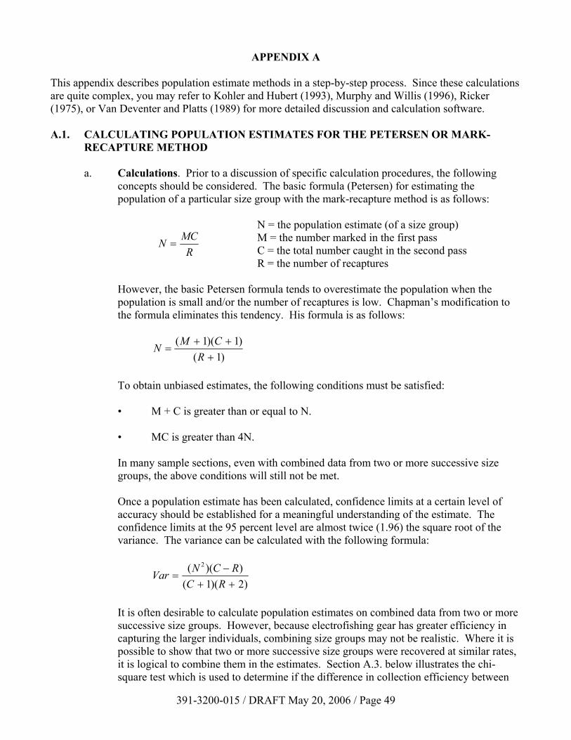
APPENDIX A This appendix describes population estimate methods in a step-by-step process. Since these calculations are quite complex, you may refer to Kohler and Hubert (1993), Murphy and Willis (1996), Ricker (1975), or Van Deventer and Platts (1989) for more detailed discussion and calculation software. A.1. CALCULATING POPULATION ESTIMATES FOR THE PETERSEN OR MARK-

RECAPTURE METHOD a. Calculations. Prior to a discussion of specific calculation procedures, the following

concepts should be considered. The basic formula (Petersen) for estimating the population of a particular size group with the mark-recapture method is as follows:

RMCN =

N = the population estimate (of a size group) M = the number marked in the first pass C = the total number caught in the second pass R = the number of recaptures

However, the basic Petersen formula tends to overestimate the population when the

population is small and/or the number of recaptures is low. Chapman’s modification to the formula eliminates this tendency. His formula is as follows:

)1()1)(1(

+++

=R

CMN

To obtain unbiased estimates, the following conditions must be satisfied: • M + C is greater than or equal to N. • MC is greater than 4N. In many sample sections, even with combined data from two or more successive size

groups, the above conditions will still not be met. Once a population estimate has been calculated, confidence limits at a certain level of

accuracy should be established for a meaningful understanding of the estimate. The confidence limits at the 95 percent level are almost twice (1.96) the square root of the variance. The variance can be calculated with the following formula:

)2)(1())(( 2

++−

=RC

RCNVar

It is often desirable to calculate population estimates on combined data from two or more

successive size groups. However, because electrofishing gear has greater efficiency in capturing the larger individuals, combining size groups may not be realistic. Where it is possible to show that two or more successive size groups were recovered at similar rates, it is logical to combine them in the estimates. Section A.3. below illustrates the chi-square test which is used to determine if the difference in collection efficiency between

391-3200-015 / DRAFT May 20, 2006 / Page 49

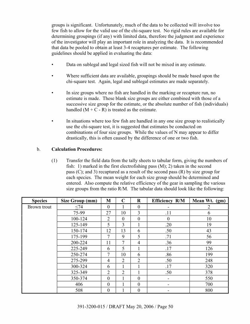
groups is significant. Unfortunately, much of the data to be collected will involve too few fish to allow for the valid use of the chi-square test. No rigid rules are available for determining groupings (if any) with limited data, therefore the judgment and experience of the investigator will play an important role in analyzing the data. It is recommended that data be pooled to obtain at least 3-4 recaptures per estimate. The following guidelines should be applied in evaluating the data:

• Data on sublegal and legal sized fish will not be mixed in any estimate. • Where sufficient data are available, groupings should be made based upon the

chi-square test. Again, legal and sublegal estimates are made separately. • In size groups where no fish are handled in the marking or recapture run, no

estimate is made. These blank size groups are either combined with those of a successive size group for the estimate, or the absolute number of fish (individuals) handled (M + C - R) is treated as the estimate.

• In situations where too few fish are handled in any one size group to realistically

use the chi-square test, it is suggested that estimates be conducted on combinations of four size groups. While the values of N may appear to differ drastically, this is often caused by the difference of one or two fish.

b. Calculation Procedures: (1) Transfer the field data from the tally sheets to tabular form, giving the numbers of

fish: 1) marked in the first electrofishing pass (M); 2) taken in the second pass (C); and 3) recaptured as a result of the second pass (R) by size group for each species. The mean weight for each size group should be determined and entered. Also compute the relative efficiency of the gear in sampling the various size groups from the ratio R/M. The tabular data should look like the following:

Species Size Group (mm) M C R Efficiency R/M Mean Wt. (gm)

Brown trout <74 0 1 0 - 2 75-99 27 10 3 .11 6 100-124 2 0 0 0 10 125-149 5 3 1 .20 19 150-174 12 13 6 .50 43 175-199 7 9 5 .71 56 200-224 11 7 4 .36 99 225-249 6 5 1 .17 126 250-274 7 10 6 .86 199 275-299 4 2 2 .50 248 300-324 6 1 1 .17 320 325-349 2 2 1 .50 378 350-374 0 1 0 - 550 406 0 1 0 - 700 508 0 1 0 - 800

391-3200-015 / DRAFT May 20, 2006 / Page 50

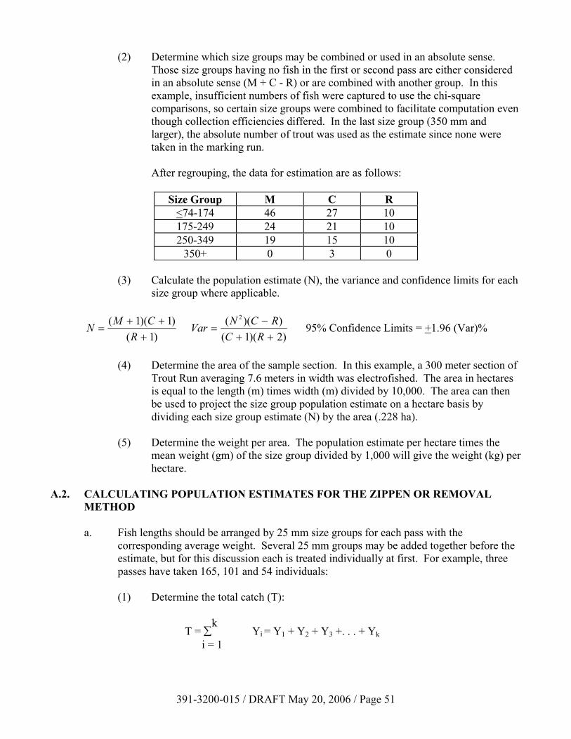
(2) Determine which size groups may be combined or used in an absolute sense. Those size groups having no fish in the first or second pass are either considered in an absolute sense (M + C - R) or are combined with another group. In this example, insufficient numbers of fish were captured to use the chi-square comparisons, so certain size groups were combined to facilitate computation even though collection efficiencies differed. In the last size group (350 mm and larger), the absolute number of trout was used as the estimate since none were taken in the marking run.

After regrouping, the data for estimation are as follows:

Size Group M C R <74-174 46 27 10 175-249 24 21 10 250-349 19 15 10

350+ 0 3 0 (3) Calculate the population estimate (N), the variance and confidence limits for each

size group where applicable.

)1()1)(1(

+++

=R

CMN )2)(1(

))(( 2

++−

=RC

RCNVar 95% Confidence Limits = +1.96 (Var)%

(4) Determine the area of the sample section. In this example, a 300 meter section of

Trout Run averaging 7.6 meters in width was electrofished. The area in hectares is equal to the length (m) times width (m) divided by 10,000. The area can then be used to project the size group population estimate on a hectare basis by dividing each size group estimate (N) by the area (.228 ha).

(5) Determine the weight per area. The population estimate per hectare times the

mean weight (gm) of the size group divided by 1,000 will give the weight (kg) per hectare.

A.2. CALCULATING POPULATION ESTIMATES FOR THE ZIPPEN OR REMOVAL

METHOD a. Fish lengths should be arranged by 25 mm size groups for each pass with the

corresponding average weight. Several 25 mm groups may be added together before the estimate, but for this discussion each is treated individually at first. For example, three passes have taken 165, 101 and 54 individuals:

(1) Determine the total catch (T):

T = ∑k

Yi = Y1 + Y2 + Y3 +. . . + Yk i = 1

391-3200-015 / DRAFT May 20, 2006 / Page 51

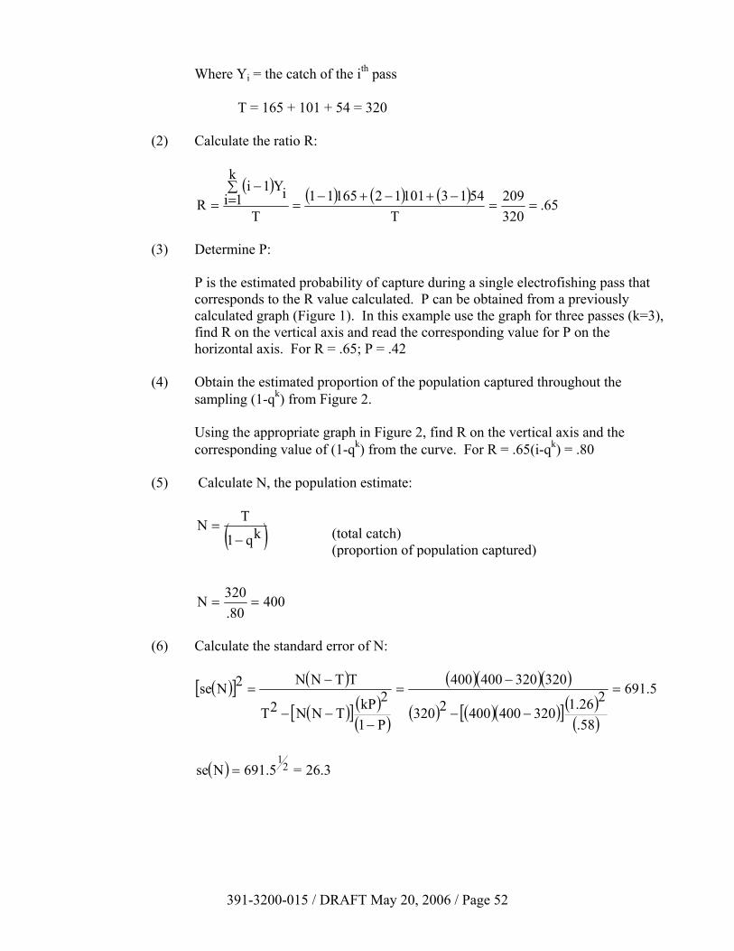
Where Yi = the catch of the ith pass T = 165 + 101 + 54 = 320 (2) Calculate the ratio R:

( ) ( ) ( ) ( ) .65320209

T54131011216511

T

k

1i iY1iR ==

−+−+−=

∑=

−=

(3) Determine P: P is the estimated probability of capture during a single electrofishing pass that

corresponds to the R value calculated. P can be obtained from a previously calculated graph (Figure 1). In this example use the graph for three passes (k=3), find R on the vertical axis and read the corresponding value for P on the horizontal axis. For R = .65; P = .42

(4) Obtain the estimated proportion of the population captured throughout the

sampling (1-qk) from Figure 2. Using the appropriate graph in Figure 2, find R on the vertical axis and the

corresponding value of (1-qk) from the curve. For R = .65(i-qk) = .80 (5) Calculate N, the population estimate:

( )kq1

TN−

=

400.80320N ==

(6) Calculate the standard

( )[ ] (

([ NN2T

NN2Nse

−

=

( ) 26.3=691.5Nse 21

=

391-3200-015 / D

(total catch) (proportion of population captured)

error of N:

)

)] ( )( )

( ) )( )(

( ) ( )( )[ ]( )( )

691.5

.58

21.263204004002320

320032400400

P1

2kPT

TT=

−−

−=

−−

−

RAFT May 20, 2006 / Page 52

(7) Calculate the confidence limits7 for N: The 95 percent confidence interval is calculated by adding and subtracting 1.96

times the standard error from the population estimate: 1.96 (26.3) = 51.5 (rounded to 52 individuals) N ± 52 = 400 ± 52 = 348 to 452

(8) With the population estimate (N), the average weights and the area of the sample section, the number and weight of fish per hectare can be determined.

7 For populations of 200 or more and when 90 percent or less is captured, the confidence limits are set at the 95th percentile level. When the population is less than 200 but greater than 50, the confidence limits are set at the 90th percentile level (substitute 1.645 for 1.96 in the equation above).

391-3200-015 / DRAFT May 20, 2006 / Page 53

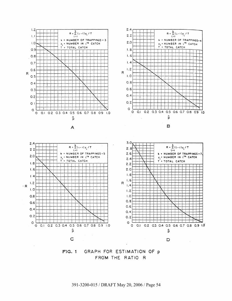
391-3200-015 / DRAFT May 20, 2006 / Page 54

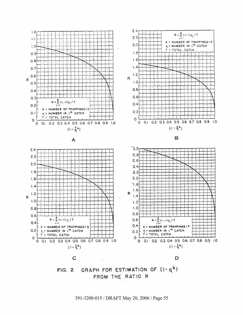
391-3200-015 / DRAFT May 20, 2006 / Page 55

A.3. Chi-Square The chi-square test determines whether observed differences in relative frequencies might have

been caused by chance alone. In this presentation, this test is used to determine if the difference in electrofishing efficiency is great enough to require separate estimates for different size groups. One assumption of the test requires an N >5 for each size group.

Background for the chi-square test can be obtained from almost any statistics textbook. An

example should suffice here. Given the following data, is the difference in electrofishing efficiency of .40 and .65 great enough to require separate population estimates for these two size groups?

Size Group M C R Efficiency

R/M 125-149 mm 25 22 10 .40 150-174 mm 20 17 13 .65

Basically, one is concerned with the recapture of marked individuals, thus the categories of data

are recaptures (R) and non-recaptures (M - R). The groups of data involved are the size classes 125 and 150.

Groups Categories

125 150 Total

Recaptures 10 13 23 Non-recaptures 15 7 22

Total 25 20 45 If there was no difference in the efficiency, then the recapture should be the same for both

groups. For both groups, a total of 23 individuals out of 45 were recaptured. Thus, with no difference in efficiency, 23/45 (or .51) of the marked individuals of either group should be recaptured. A second table is constructed expressing the actual data (observed) and hypothetical data (expected, i.e., no difference in efficiency). The .51 is applied to the total number marked in each group to determine the expected number of recaptures. Thus, in the 125 mm group (.51 x 25 = 13), 13 marked individuals should have been recaptured and (25 - 13) or 12 missed. The same .51 recapture rate when applied to the 150 mm group showed 10 individuals should have been recaptured (20-10) and/or 10 missed.

Groups Categories Observed Expected (O-E) (O-E)2 (O-E)2 / E

125 Recapture 10 13 -3 9 .6923 Non-recapture 15 12 3 9 .75

150 Recapture 13 10 3 9 .90 Non-recapture 7 10 -3 9 .90 Total 45 45 Σ=3.2423=X2

When reviewing the hypothesis tested that there is no significant difference between efficiencies,

one must compare the calculated chi-square value with a critical tabular one. With the

391-3200-015 / DRAFT May 20, 2006 / Page 56

accompanying table, find the X2 value for the corresponding degrees of freedom, (the number of groups -1) times (number of categories -1) or 1 in this case.

If the calculated chi-square value is greater than the tabular one, the hypothesis must be rejected

and the difference in efficiency is significant. If the calculated chi-square value is less than the tabular value, the difference is not statistically significant. In the example, the calculated chi-square value of 3.2423 is less than the tabular value of 3.84146. Thus the efficiency for the 125 and 150 mm size groups was not significantly different, and the two groups could be combined if so desired.

Chi-square may be used to test multinomial populations (having two or more categories) and to

test more than two populations or groups. The basic method discussed above is essentially the same.

Table of Chi-Square Distribution

Degrees of freedom

Region of hypothesis rejection at 5% significance

when computed X2 value is greater than

Degrees of freedom

Region of hypothesis rejection at 5% significance

when computed X2 value is greater than

1 3.84146 16 26.2962 2 5.99147 17 27.5871 3 7.81473 18 28.8693 4 9.48773 19 30.1435 5 11.0705 20 31.4104 6 12.5916 25 37.6525 7 14.0671 30 43.7729 8 15.5073 40 55.7585 9 16.9190 50 67.5048 10 18.3070 60 79.0819 11 19.6751 70 90.5312 12 21.0261 80 101.879 13 22.3621 90 113.145 14 23.6848 100 124.342 15 24.9958

391-3200-015 / DRAFT May 20, 2006 / Page 57

APPENDIX B

Introduction to Basic Electrofishing Techniques

Background. Many DEP & PFBC personnel attended the United States Fish and Wildlife Service (USFW) electrofishing (EF) course (“Principles and Techniques of Electrofishing”) offered at PSU - State College during the summer of 1994. This 3-day course was “heavy” on electrical theory, EF boat wiring design and related safety issues. Outdoor simulations were at a nearby lake involving measurements of EF boat electrical fields and very little concerning backpack units. While regional biologists may occasionally employ EF boats, the most common EF collections are in wadeable streams using backpacks. There were virtually no presentations concerning backpack/wading issues at the USFW ‘94 course. Many of the attendees felt the USFW course did not adequately address their EF backpack needs. Need: There are many career biologists in state employment. During the early 70’s there were approximately seven DEP (then DER) Water Pollution Biologists (WPBs) covering regional field duties. There were many Water Quality Specialists (WQS) in the regions as well. The WQSs often provided EF assistance. This has not changed. However, DEP’s number of WPBs and WQSs has grown considerably. This has resulted in a wide spectrum of EF experience (<1 year - 20+ years) in both WPB and WQS ranks. The experienced WPBs and WQSs are well versed in EF techniques and “mechanics” and have developed their own individual styles. Many of the newer WPBs and WQSs need basic “hands-on” EF experience. They are at a disadvantage when they join experienced (or PFBC) crews or need to form EF crews and conduct their own EF surveys. Scope: The scope of this session is to present basic, generally accepted EF technique mechanics and advise field staff of DEP’s official electrofishing document (Attachment A- 5/1/97; technical guidance DEP ID: 400-5900-116). It is geared towards DEP’s “new hires” or field staff who, on occasion, may assist in EF collection efforts.

Disclaimer: There are no “official” statewide EF practices, nor does this session intend to instill such official practices beyond the scope of the aforementioned 5/1/97 technical guidance (Attachment A). It shall be the responsibility of all EF participants to familiarize themselves with DEP’s EF technical guidance document. The information presented in this session is intended as recommendations based on the experience of many of the longer termed WPBs. This session is not intended to provide a basic overview of electrical theory or EF boating principles, nor is it intended to replace the need to attend USFW’s EF course. Further, while basic wader safety issues will be addressed, this session does not replace the need to attend PFBC’s water and boating safety course.

Basic Electrofishing Considerations

1. EF backpack & probe design issues a) Backpacks: There are several backpack designs commonly used for EF surveys. Two

common ones used by Pennsylvania state agencies are gas engine generated “Coffelts” and battery powered “Smith Roots.” Whatever system is chosen, the backpack frame should be made of strong, light-weight, non-metallic material. (Recommended: shoulder straps should have a “quick-release” design in the event of submersion.)

391-3200-015 / DRAFT May 20, 2006 / Page 58

b. Gas engine units (e.g., Coffelt units): Uses a gas-powered generator and two hand-held

probes or one hand-held probe and a rat-tail (or metal mesh screen) probe that drags behind the unit.

i) Advantages: AC, DC, DC pulse electricity generation options available; simple

watt-meter; switch controls are simple to operate; normally lighter than battery units; gas engine is usually very dependable.

ii) Disadvantages: inherent dangers working/transporting/storing gasoline;

occasional gas tank seepage with leaning; running out of gas in the middle of a segment.

c. Smith-Root: Electric battery powered and has one hand-held probe, with the other probe

being a heavy wire terminal that drags along behind the unit. i) Advantages: has an automatic “tilt” shut-off switch; “One-man” operation

possible (but NOT ENCOURAGED); has a cumulative “electricity-on” counter (in seconds); built-in “beeper” that pulses at a specific rate when generating in the “optimally effective” shocking range; quieter.

ii) Disadvantages: heavier than gas units; requires battery charger; limitations to

shape of “electric field barrier”; settings adjustments are not readily understandable; potential for acid burns to skin and clothing.

d) Probes: Are usually equipped with round or diamond-shaped hoops and thumb switches.

For the probes to conduct their electrical charge, both switches must be depressed at the same time. The mechanical action of these thumb switches can be quite variable. Some switches are hard to depress for long periods of time -- causing rapid fatigue to the probe forearm. In some cases, these have been modified by taping tongue depressors (or similar paddle-shaped item) over the switch that requires a full hand-grip to engage the switch. Others have often simply taped the switches down so that they are permanently on. In some cases, you may encounter probe sets that were “directly wired” -- bypassing the switches and rendering them permanently on. In both cases, on/off operation is accomplished by simply lifting one probe out of the water. While there are advantages and convenience to having the probes on permanently, it is NOT RECOMMENDED when working with inexperienced personnel, for obvious safety reasons. Such modifications defeat the “passive” safety concept of the switch design and convert it to an “active” safety concept. In other words, with operable switches, no effort (passive) is required to create a “safe” condition (no electrically charged water by default) when not actively electrofishing. Whereas with “directly wired” designs, the water is electrically charged by default and effort must be made (active) to break the electric field in emergencies (i.e., recognizing the dangerous situation and then reacting to lift the probe out of the water in time). Further, with “directly wired” scenarios, the probes are constantly “live” and dangerous while the backpack unit is on.

391-3200-015 / DRAFT May 20, 2006 / Page 59

2. Electrofishing Results (effectiveness): Three main factors that influence efficiency are fish characteristics, habitat and operating conditions (EF equipment and crew).

a. Fish Factors: Fish response (or “are you zapping ‘em . . .”) to EF is dependent on

species, life cycle stage, individual’s size, tissue conductivity, fish scale size (large offering more resistance).

b. Habitat factors: Include water conductivity, depth and substrate type. c. Operating conditions: EF equipment considerations; such as power source, electrode

design and electrical waveform (smooth DC, pulsed DC, AC) are important factors. Crew experience, size and attitude also must be factored in for optimal safety and success.

AC/DC safety issues: DC (smooth and pulsed) - smooth wave DC is least injurious to

fish. Pulsed DC injuries are more variable; being more severe in certain larger individuals. With the use of DC, fish tend to align themselves in the electrical field and “swim” towards the anode. Their reaction is more predictable. Fishes have a greater chance of recovery and minimal injury. AC is generally more damaging to fish because of the alternating polarity. Due to the rapid changes in polarity, the fish can’t align in one direction and approach the anode, resulting in very unpredictable reactions. Fish may display advanced oscillotaxis (rigid, quivering muscles) that can lead to serious internal injuries and higher mortality rates.

3. Gear requirements • Chest waders (felt soles or cleats) • Hip boots (felt soles or cleats) • Rubber insulating gloves (elbow length) • Nets (long and short, non-metallic handles) • Buckets (plastic) • Polarized glasses a. The primary EF crew must* wear chest waders and gloves to allow excursions into

deeper pool areas. Chest waders are most critical to the backpacker. While full immersion would negate the advantage offered by the chest waders, they could offer effective protection with lesser slipping and falling mishaps.

b. Secondary, or support EF crew members should also wear chest waders but could get by

with hip boots. Knee length boots are not recommended because of their limited versatility. At no time should any assistants be allowed to “wet wade” or wear wading shoes only.

*In smaller, very shallow streams, chest waders should still be the boot of choice.

However, hip boots would be acceptable.

391-3200-015 / DRAFT May 20, 2006 / Page 60

4. Crew member responsibilities a. Project Leader: Usually the biologist who needs the data. Therefore, the project leader

will determine the type and level of EF effort necessary (qualitative, cursory check list to quantitative, intensive removal of all stunned fish).

b. Primary EF Crew i) Team Leader: conducts a “pre-game” - briefing on techniques, equipment and

expectations will be discussed (may often be crew member #1). (1) Crew member #1 (backpacker, prober and netter): Reviews team

configuration (net and probe pattern, assistants’ placement; strategy, signals (verbal or otherwise); starts timing the EF level of effort; and once the water is electrified, “runs the show” - guiding and directing the advancing EF crew to maintain the EF barrier).

(2) Crew member #2 (prober, if necessary, and netter): Parallels #1 and

follows lead; assists #1 in navigating around, under, over obstacles; responsible for own “half” of EF field.

Even though each prober works their probe “independently,” they must

keep the probes submerged while turning to dump fish in a bucket so that their partner can continue to net stunned fish uninterruptedly.

(3) Crew member #3 (netter and bucket carrier): Follows behind between #s

1 & 2, attempting to net missed fish; presents bucket to #s 1 & 2 when necessary, elevated with handle tipped back; monitors EF unit’s watt-meter and adjusts voltage upon request.

c. Secondary EF crew (optional) Netters and bucket carriers: Stationed further behind and to the sides of Primary crew;

assist in netting missed fish and transferring fish to instream live wells of larger holding buckets for data processing.

5. Managing the electrical field and associated barrier The probe handlers are directly responsible for maintaining an effective electrical field. Each

handler has primary responsibility for their own probe and must scan and net fish stunned by his/her own probe. If “business is slow” then the handler can expand his/her scanning field of vision and assist with the stream area that is common to both handlers.

During the steady advancement upstream, the probes must be kept submerged with switches

depressed to maintain the electrical field. It is important for all probe handlers to realize that besides stunning fish for netting, the electrical field also creates a barrier. A fish’s first reaction to “tingles” may be to momentarily hide or attempt to flee ahead of the advancing EF team. This will often “herd” the fish upstream until they encounter a physical barrier. Once they do, they may attempt an “end run” downstream (around the weaker, outer fringe of the EF field. As long

391-3200-015 / DRAFT May 20, 2006 / Page 61

as the electrical barrier has been constantly maintained with proper distance between the probes, most will be unable to escape without being stunned. The briefest electrical interruption (switches off or probe out of the water) may allow many to escape.

During certain surveys, maintaining a constant electrical barrier may not be important, no matter

how wide the stream is (simple, cursory EF passes intended to collect representative taxa presence/absence data or fish tissue specimens). However, for most surveys, quantitative data is the objective (population estimates, biomass calculations, IBI metrics surveys, etc.). In these cases, it is necessary to collect all specimens possible and electrical barrier management becomes a critical factor.

Note: Some investigators find that the electrical field formed by DC output may not create a very effective barrier to fish passage when moving upstream unless the positive probes are used to create the field. In cases where a Coffelt unit is being used, the handlers using the negative probes should “lag behind” the positive probe handlers so that the + probes can form a barrier. This can be more difficult to accomplish in streams of substantial width. The negative probes will stun some fish, but will allow many to escape. With a Smith-Root unit, the negative probe trails behind so the + probes form the field. There is a trade-off between AC & DC. AC can be more efficient in catching fish, but is also more harmful to the fish’s well being. With DC, efficiency may be sacrificed for fish survival.

6. Instream probe movement patterns - 2-, 3-, multi-crew issues Normally, for small streams, the advancement pattern is a simple, side-by-side walk straight up

the middle of the stream. The EF barrier would effectively “bulldoze” the fish upstream. For moderately wider streams, it will be necessary to modify this pattern. Experienced #1 and #2 crewmembers can effectively do the same thing by carefully “pivoting” their EF barrier from side-to-side in a zig-zag pattern. In very wide streams, a second EF crew may be necessary to shock in tandem to form overlapping EF barriers. Each crew would be responsible for its half of the stream and must work together in a coordinated manner to reduce or minimize the number of “escapees.”

7. Deeper, hidden, murky areas and fast currents pose special EF problems. Shocking pools and

undercut banks will often “kick out” many “lunkers” and trigger brief, frantic excitement - often eliciting primal instinctual sound effects among the crewmembers. Often, there are many escapees because of this unsuspected surprise. The backpacker (crewmember #1) should advise the others on positioning and strategy when attempting to shock these productive habitats.

8. Fish mortality issues

All reasonable efforts should be made to minimize fish injury and mortality when possible. The

EF survey type may allow for release of extra fish (fish tissue surveys, qualitative field IDs). If extra game fish are collected that do not need to be preserved, they should be processed first and released quickly to reduce temperature and DO related stresses.

Note: If fish mortality does occur, do not carelessly dispose of fish in the field. The public perception of fish killed and wasted by a resource protection agency is not a good image. If you can’t discretely dispose of dead fish in the field, take them with you as part of your “collection” even if you plan to discard them later.

391-3200-015 / DRAFT May 20, 2006 / Page 62

9. Deep pool and instream obstacle considerations These features present special safety concerns. Deep pools would require chest waders and

longer handled nets to reduce risk of submersion. Obstacles also present problems. Excessive leaning to crawl over large logs or under low hanging vegetation can tilt the shocker, causing it to “cut out.” When navigating such obstacles, it may be necessary to interrupt the EF barrier by releasing the probe switches. Sometimes it will be necessary to “portage” around large obstacles.

10. Complying with DEP’s EF guidelines

DEP has a technical guidance document available on DEP’s Web site entitled Policy for Electrofishing Personnel and Equipment Safety, DEP ID: 400-5900-116, available on DEP’s Web site. It outlines other important EF safety guidance issues beyond those discussed above. Each crewmember should be provided a copy of this document and Attachment A for their review and understanding. This presentation is intended to emphasize safety aspects of EF by providing an overview presentation of common EF mechanics. It is not intended to substitute for other EF guidelines or available courses (i.e., USFW’s “Principles and Techniques of Electrofishing”). Nor should DEP staff avoid taking other EF training or water-related safety courses.

11. Other safety issues Because of the inherent dangers of EF, everyone involved must be proactive and anticipate

“worst-case” scenarios. This would apply to any field survey activities; no matter how remote they are. A contingency plan for emergencies should be formulated, presented by the Project Leader and discussed. For example, the following issues should be considered:

• Be alert to spectators, pets or livestock entering the water in your EF segment and

forewarn, if appropriately necessary. If they are near the stream, anticipate that they may enter the water accidentally.

• Does anyone have a cell phone? Is there local coverage? • Do all participants know where they are - meaning, if the crew member most familiar

with the area is rendered uncommunicative due to injury, allergic reaction or other medical emergency -- will someone be able to navigate their way for help and return?

• Does anyone have a potential threatening medical condition? • Is there a first-aid kit available? • Who has extra vehicle keys? 12. Collector’s permit

The Pennsylvania Fish & Boat Commission (PFBC) requires that anyone collecting fish other than by recreational angling must possess a PFBC issued collector’s permit. According to collector permit requirements, assistants should be listed on the collector’s permit. Also, you may be required to notify PFBC when you conduct EF surveys.

391-3200-015 / DRAFT May 20, 2006 / Page 63

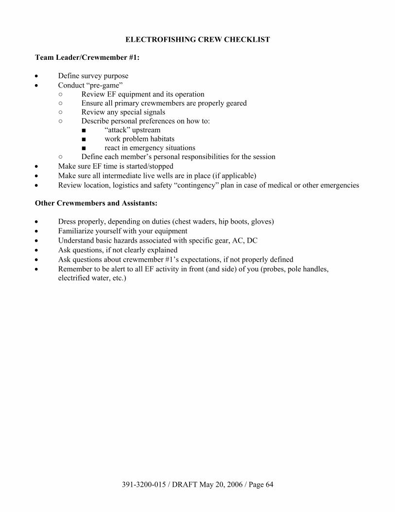
391-3200-015 / DRAFT May 20, 2006 / Page 64

ELECTROFISHING CREW CHECKLIST Team Leader/Crewmember #1: • Define survey purpose • Conduct “pre-game” ○ Review EF equipment and its operation ○ Ensure all primary crewmembers are properly geared ○ Review any special signals ○ Describe personal preferences on how to: ■ “attack” upstream ■ work problem habitats ■ react in emergency situations ○ Define each member’s personal responsibilities for the session • Make sure EF time is started/stopped • Make sure all intermediate live wells are in place (if applicable) • Review location, logistics and safety “contingency” plan in case of medical or other emergencies Other Crewmembers and Assistants: • Dress properly, depending on duties (chest waders, hip boots, gloves) • Familiarize yourself with your equipment • Understand basic hazards associated with specific gear, AC, DC • Ask questions, if not clearly explained • Ask questions about crewmember #1’s expectations, if not properly defined • Remember to be alert to all EF activity in front (and side) of you (probes, pole handles,

electrified water, etc.)