AU

MU

a

ARRA

KCDR

1

taisiiu1(fcfobmdw

r0

r

0d

Forest Ecology and Management 260 (2010) 1613–1622

Contents lists available at ScienceDirect

Forest Ecology and Management

journa l homepage: www.e lsev ier .com/ locate / foreco

stand density index for complex mixed species forests in the northeasternnited States

ark J. Ducey ∗, Rachel A. Knappniversity of New Hampshire, Department of Natural Resources and the Environment, Durham, NH 03824, USA

r t i c l e i n f o

rticle history:eceived 9 May 2010eceived in revised form 6 August 2010ccepted 11 August 2010

a b s t r a c t

Quantifying stand density is important for accurate prediction of net biomass and carbon accumula-tion, for estimating growth and mortality risks of trees, stands, and regions, and for the management offorests for multiple goods and services. Building on previous work relating maximum stand density towood specific gravity, we develop a stand density equation for the mixed species forests of the north-

eywords:ompetitionensity managementelative density

eastern United States using data from the US Forest Service, Forest Inventory and Analysis program. Weused quantile regression, in concert with a quantile selection and evaluation procedure, to ensure con-formity between our density measure and previously developed guidance for well-studied stand types.The resulting strictly additive relative density measure appears to provide reasonable prediction of max-imum density even for plantations of exotic conifers in the region. The results suggest that maximumstand densities after accounting for wood specific gravity may be lower in northeastern North Americathan in the south or west.

. Introduction

The forests of northeastern North America include tree specieshat differ greatly in growth rate, shade tolerance, and competitivebility. This makes analysis, silvicultural prescription, and model-ng of these mixed forests difficult. A key stand attribute for bothilvicultural and strategic-scale assessment of forest characteristicss stand density (Long, 1985; Woodall et al., 2005). Stand densitys important not only for evaluating carbon sequestration and vol-me development due to ordinary stand development (Assmann,970), but also for evaluating risks due to abiotic factors such as fireWoodall et al., 2006) and wind (Lindroth et al., 2009) and bioticactors such as insect outbreaks (Kurz et al., 2008). For broad appli-ability within a region comprised of heterogeneous mixed-speciesorests, a density measure must be able to contend with a rangef diameter distributions and species compositions. It should also

e able to accommodate rare species. In the context of local standanagement, a new stand density measure should avoid contra-

iction of accepted and successful empirical density measures fromell-studied monocultures. However, for large-scale regional and

∗ Corresponding author at: University of New Hampshire, Department of Natu-al Resources and the Environment, 114 James Hall, 56 College Road, Durham, NH3824-3589, USA. Tel.: +1 603 862 4429; fax: +1 603 862 4976.

E-mail addresses: mjducey@cisunix.unh.edu (M.J. Ducey),al39@unh.edu (R.A. Knapp).

378-1127/$ – see front matter © 2010 Elsevier B.V. All rights reserved.oi:10.1016/j.foreco.2010.08.014

© 2010 Elsevier B.V. All rights reserved.

national density assessments, such conflicts might be less impor-tant, with national consistency being more important than localaccuracy. Straightforward statistical procedures should be used,to allow periodic checking and (if necessary) refitting as condi-tions (such as changes in climate or species composition) warrant.Finally, it would be desirable (though not mandatory) if the den-sity measure had a reasonably simple mathematical form, in orderto facilitate modeling and to enable straightforward evaluation ofsampling error and other forms of uncertainty (Ducey and Larson,2003).

Unfortunately, while there is abundant literature on measuringstand density in single-species stands or in simple and regionallycommon species mixtures, approaches suitable for complex standsin regions with large numbers of tree species have been relativelyfew (Woodall et al., 2005). Here we develop a relative density mea-sure for use in mixed species stands in the northeastern region ofthe United States including Maine, New York, Vermont, New Hamp-shire, Massachusetts, Connecticut, and Rhode Island. Our approachbuilds on the tree-area ratio method of Chisman and Schumacher(1940), and earlier work by Stout and Nyland (1986), Stout et al.(1987), and Woodall et al. (2005). It employs a formulation closelyrelated to that of Reineke (1933), which Zeide (2005) describes as

one of the best available measures for describing the stand densityof monocultures. A particular advantage of our approach is the useof a quantile regression technique in the parameter estimation andselection process. This technique enables us to ensure conformitybetween our new, mixed-species stand density measure and that

1 y and

dr

2

sbdamt

l

ww(

S

oooomteasPdvfs

css1t(rf

A

wiDcrNLlnu

scPli((

614 M.J. Ducey, R.A. Knapp / Forest Ecolog

eveloped by previous authors for well-studied stand types in theegion.

. Theory

Reineke (1933) described a method of determining density oftocking in even-aged forests that is based on the relationshipetween number of trees per unit area and the quadratic meaniameter (QMD) of the stand. He found that single species, even-ged stands of trees at normal density (or maximum density, aseasured using relatively large growth and yield plots) conform to

he following relationship:

og N = −1.605 log QMD + k (1)

here N is number of trees per hectare and k is a constant varyingith species. Reineke (1933) also developed a Stand Density Index

SDI),

DI = N(

QMD25.4

)1.605(2)

By comparing the value of SDI calculated using Eq. (2) usingbserved values of N and QMD for a stand, with the value of Nbtained by substituting a reference diameter (25.4 cm in Reineke’sriginal work) into Eq. (1) (i.e., the maximum SDI for the species),ne can compare the actual density of a stand with that of a nor-ally stocked stand having the same species composition. Note

hat the coefficient 1.605 was obtained by Reineke (1933) by visualstimation using logarithmic graph paper. Other researchers, usingvariety of data sources, have also found estimates near 1.6, thoughome have noted slight variations between species. For example,retzsch and Biber (2005) found that several species in their studyiffered in slope coefficient from each other and from the nominalalue of 1.6. However, Reineke’s (1933) general formulation hasound widespread application, particularly for even-aged single-pecies stands (Shaw, 2000; Woodall et al., 2005; Shaw, 2006).

Reineke’s (1933) original index was developed within theonceptual framework of normally stocked, single-cohort, single-pecies stands. Normal stocking implies maximum density at thetand scale, akin to the A-line in stocking diagrams (cf. Gingrich,967). Application of Reineke’s approach to mixed-species or mul-iple cohort stands has proven challenging (Shaw, 2000). Curtis1970, 1971) developed a power-law density measure closelyelated to SDI, which was reformulated by Long and Daniel (1990)or use in mixed-age stands:

SDI =∑

i

Ni

(DBHi

25

)1.6(3)

here ASDI is the alternative or additive formulation of SDI, Nis the number of trees per hectare in the ith diameter class, andBHi is the diameter of trees in that class. When dealing with aontinuous diameter distribution, the summation in Eq. (3) can beeplaced by an integral, and Ni can be replaced by the product of

and an appropriate probability density function (cf. Ducey andarson, 2003). ASDI has been suggested as a useful tool for irregu-ar and multicohort stands (Long, 1995; Shaw, 2000). However, theeed to establish a maximum density for comparison has made itsse in mixed-species stands difficult.

Several recent studies have explored SDI and related den-ity measures for relatively simple, well-defined species mixturesonsisting of only a few major component species. For example,

uettmann et al. (1992) extended the concept of the self-thinningine (Yoda et al., 1963), typically applied to monocultures, to exam-ne mixtures of Douglas fir (Pseudotsuga menziesii) and red alderAlnus rubra). Pretzsch (2005) examined mixtures of Norway sprucePicea abies) and European beech (Fagus sylvatica). Other recent

Management 260 (2010) 1613–1622

studies have examined western hemlock (Tsuga heterophylla) andSitka spruce (Picea sitchensis) (Poage et al., 2007), western hem-lock and douglas-fir (Pseudotsuga menziesii) (de Montigny and Nigh,2007), spruce-pine-fir (Picea-Pinus-Abies spp.) and poplar (Popu-lus spp.) (Penner, 2008). However, in species-rich regions such asnortheastern North America, forests do not always occur as pre-dictable mixtures and the number of species cooccurring in anystand can be large (at least by temperate forest standards).

Woodall et al. (2005) suggest an alternative approach for usingSDI in mixed-species stands that builds on earlier mechanistic workby Dean and Baldwin (1996). Dean and Baldwin (1996) noted thatthe maximum stand density of single-species stands was negativelycorrelated with wood specific gravity. Specific gravity, in turn, is apowerful predictor of other wood mechanical properties. For twostands with the same QMD but of different species, the stand com-prised of trees with denser and stronger wood should support morefoliage biomass per tree. All other things being equal, then, it shouldrequire fewer trees (and hence a lower SDI) to completely occupya stand if trees have denser and stronger stems, implying that themaximum SDI for species with high specific gravity will be lowerthan that of species with low specific gravity. Woodall et al. (2005)developed this observation into a predictive relationship,

E[SDImax] = a0 + a1(SG) (4)

where E[SDImax] is the expected maximum value of ASDI for themixture, a0 and a1 are empirical coefficients (with a1 negative),and SG is the mean specific gravity of trees in the stand. Woodall etal. (2005) develop their equation using ASDI as the primary densitymeasure. However, if we use

Relative density = ASDIE[SDImax]

(5)

to compare stands of different composition (Woodall et al., 2006),the relative density is not additive (in the sense that ASDI is; Duceyand Larson, 1997) but merely separable (sensu Ducey and Larson,2003). This can lead to minor annoyances, including bias whenestimating stand density from a small sample (Ducey and Larson,1999). Also, the density contribution of a tree or group of treesdepends on the composition of the entire stand, through the effectof stand average specific gravity on E[SDImax].

As an alternative, consider the general approach of Chisman andSchumacher (1940). They supposed the growing space requirementof an individual tree at normal stocking would be well representedby a quadratic equation, i.e.

Ai = c0 + c1DBHi + c2(DBHi)2 (6)

where Ai is the growing space requirement of the ith tree, DBHi isthe diameter at breast height of the ith tree, and c0, c1 and c2 arecoefficients. The total growing space requirement of trees in a stand(the “tree area ratio,” or TAR) would be

TAR = c0N + c1

∑i

DBHi + c2

∑i

(DBHi)2 (7)

where the summation is over all the trees in a unit area. Chismanand Schumacher (1940) recognized that if stands were selected apriori to have normal stocking, then (with appropriate selection ofunits) TAR could be set to 1, and the parameters could be estimatedusing data from multiple plots by ordinary least-squares regres-sion. If observed stand values are then used in Eq. (7), the resultis the density of the stand as a fraction of normal stocking. Stout

et al. (1987) generalized this approach to a mixed-species situa-tion. Ideally, because of different space requirements, each specieswould have its own values of c0, c1, and c2, but this would lead to avery large number of estimated parameters. For rare species, theremight be insufficient numbers of trees to obtain stable parameter

y and

eo

m

A

w(iahBs

c

i

wm

e“Fobrwa(csed

Snsrwsts

3

3

F2nIhaBstf

M.J. Ducey, R.A. Knapp / Forest Ecolog

stimates. As a result, Stout et al. (1987) employed a small numberf species groups rather than individual species.

We propose to follow Curtis (1971) in using an exponential for-ulation of Ai,

i = c1

(DBHi

25

)1.6(8)

here c1 is a species-specific parameter. We have followed Long1985) in setting the reference diameter to 25 cm, rather than insist-ng on the original 25.4 cm (10 in.) value of Reineke (1933), and havessumed an even 1.6 for the exponent (which, for our purposesere, is taken to be species-invariant). We further follow Dean andaldwin (1996) and Woodall et al. (2005) in relating c1 to the woodpecific gravity of the tree,

1 = b0 + b1SGi (9)

Combining Eqs. (8) with (9) and adding over all measured treesn the stand gives a relative density measure akin to TAR,

RD =∑

i

(b0 + b1SGi)(

DBHi

25

)1.6

= b0

∑i

(DBHi

25

)1.6+ b1

∑i

SGi

(DBHi

25

)1.6 (10)

hich has only two estimable parameters, b0 and b1, no matter howany species are under consideration.Note that RD is scaled so that RD = 0 represents a completely

mpty stand, and RD = 1 represents a stocking level consistent withnormal” or A-line stocking using conventional stocking guides.ollowing Stout et al. (1987), we do not take the contributionf individual trees to RD to reflect two-dimensional crown area,ut rather the proportional consumption of potentially limitingesources in general. By its construction, RD is additive in the sameay that TAR and the Stout et al. (1987) density measure are (Ducey

nd Larson, 1997). Thus, the density contribution of groups of treeswhether described by diameter ranges, by species, or both) can bealculated independently of the contents of the remainder of thetand. This contrasts with the relative density measure of Woodallt al. (2006), for which the density contribution of a group of treesepends on the average specific gravity of all trees in the stand.

If, following Chisman and Schumacher (1940), Curtis (1971), andtout et al. (1987), we were able to select only stands meeting theormal or reference density criterion, then Eq. (10) could be fit byetting RD to 1 for every stand and using ordinary least-squaresegression. In our application, we cannot select our data a priori, bute will suggest an approach for fitting (10) using quantile regres-

ion, with the quantiles selected to ensure compatibility betweenhe mixed-species density measure and existing single-species orimple-mixture guidelines for the region.

. Methods

.1. Data

We used data collected as part of the USDA Forest Service’sorest Inventory and Analysis (FIA) program between 1983 and007. The tree tables for our study area which includes Con-ecticut, Maine, Massachusetts, New Hampshire, New York, Rhode

sland and Vermont were downloaded from the FIA websitettp://www.fia.fs.fed.us/ [accessed on 18 Sept 2008, except VT

ccessed on 28 Nov 2007]. For full details on the FIA program, seeechtold and Patterson (2005). The tree table includes all mea-ured trees with DBH >12.5 cm. Dead trees were removed fromhe dataset. Also, all plots containing trees with missing expansionactors were excluded from the analysis.

Management 260 (2010) 1613–1622 1615

The tree level data from the FIA database included species iden-tification, diameter at breast height, and a tree expansion factor.We tabulated wood specific gravities for all species appearing inthe data from published sources (Appendix A). Our list differs fromthe recently published work by Miles and Smith (2009) in includ-ing some additional species, and in a few cases there are minordifferences in reported specific gravities. In those few cases wherespecific gravity was not available, we estimated it based on thespecific gravities of other species in the same genus. For unknownconifers and unknown broadleaved trees we calculated the medianconifer specific gravity and the median broadleaved specific grav-ity, respectively. The database included species ranging from a lowof 0.31 (northern white cedar) to a high of 0.84 (Osage-orange).Although specific gravity values can vary within a tree speciesand even within an individual tree, we adopted a uniform specificgravity for each species for the purposes of fitting the model. Weused specific gravity with volumes measured at a moisture contentof 12%, because we found the greatest number of known values.This moisture content is considered an average air-dry conditionreached without artificial heating (Markwardt, 1930), For a smallnumber of species, specific gravity at 12% moisture content wasunavailable and we estimated that value from specific gravity withvolume measured when green, based on a regression correctiondeveloped from species where both values were available.

For each plot, we calculated the two summands in Eq. (10),using the expansion factors (EFi) from the database (after metricconversion) to scale each tree to a unit hectare, viz.

x0 =∑

i

EFi(DBHi)1.6

x1 =∑

i

EFiSGi

(DBHi

25

)1.6 (11)

We treated entire cluster plots, rather than subplots, as standswhenever the FIA design involved cluster plots, and ignored themapping of forest and nonforest areas in the current annual-ized design. The study period and region does span the transitionbetween the periodic and annual FIA design, and includes bothfixed- and variable-radius plots in the periodic design. We repeatedthe statistical analyses outlined below using a subset of the datafrom the more recent fixed area sampling design, and the resultsdid not differ appreciably from those obtained using the full dataset.Therefore, the full dataset was used for final analysis.

3.2. Quantile regression

A variety of statistical techniques have been used to identifymaximum or normal density levels, including ocular estimation(Reineke, 1933), ordinary least squares (Chisman and Schumacher,1940), reduced major axis regression (Solomon and Zhang, 2002),quantile regression and segmented regression (Zhang et al., 2005),stochastic frontier functions (Bi, 2004; Zhang et al., 2005; deMontigny and Nigh, 2007; Weiskittel et al., 2009), and mixed-effects models (VanderSchaaf and Burkhart, 2007). Within the treearea ratio framework of Chisman and Schumacher (1940), nearlyall published work has used ordinary least squares.

Suppose, following Chisman and Schumacher (1940), we setRD = 1 for all stands in order to estimate parameters. Let us rewriteEq. (10) using the simplifications in Eq. (11), and with an expliciterror term:

b0x0 + b1x1 + ε = 1 (12)

Ordinary least squares would choose the parameter values thatminimize the sum of squared errors, i.e.

SSE =∑

(1 − b0x0 − b1x1)2 (13)

1 y and

dsttswgwc(ic

(hoooiw

mdv

�

wtcoqbis2tds

3

rdirooab(ptectTpoAatb

t

616 M.J. Ducey, R.A. Knapp / Forest Ecolog

Ordinary least squares assumes the error term is normallyistributed (in the statistical sense, not in the sense of “normaltocking”), and selects parameters so that the mean of the errorerm is zero. It is not easy to motivate the first assumption even ifhe data have been prescreened to include only normally stockedtands. But if the data have been prescreened, ordinary least squaresould provide parameter estimates so that equation [10] would

ive RD = 1 for an average normally stocked stand. The challengeith many data sources, including FIA data, is prescreening which

an introduce subjectivity and variability into the modeling processZhang et al., 2005). If the data have not been prescreened, theres no reason to believe that the average stocking level in the dataorresponds to the stocking level for which RD = 1 is desired.

Instead of ordinary least squares, we used quantile regressionKoenker and Bassett, 1978; Koenker, 2005). Quantile regressionas been suggested for finding boundaries or envelopes in a varietyf ecological settings (Scharf et al., 1998; Cade and Noon, 2003). Inur context, it does not require the subjective selection of a subsetf the data based on predefined criteria (Zhang et al., 2005), and it isnsensitive to the presence of extreme outliers (Scharf et al., 1998),

hich is helpful in dealing with very large data sets.Quantile regression chooses the parameters so that they mini-

ize a weighted sum of absolute values of errors, where the weightepends on whether the error is positive or negative. For an indi-idual observation,

�(ε) = ε[� − I(ε < 0)] (14)

here � is a predetermined quantile between 0 and 1. The func-ion I(ε < 0) = 1 if ε < 0, and I(ε < 0) = 0 otherwise. Quantile regressionhooses the parameters that minimize the sum of the ��(ε) over allbservations. In so doing, it chooses parameters such that the �thuantile of ε will be zero, and the fraction of observations that fallelow their predicted values will be �. If � = 0.5, quantile regression

s simply least absolute deviation regression and quantile regres-ion finds a relationship such that the median error is zero (Koenker,005). In our context, quantile regression finds a relationship suchhat RD = 1 describes the �th quantile of density within the entireata set. If � is set very close to one, the parameters will be choseno that RD = 1 describes the upper limit of observed density.

.3. Quantile evaluation and selection

But is the upper limit of observed density really the desiredeference density RD = 1? Much of the literature on fitting standensity models, going back to Reineke (1933) has focused on find-

ng the maximum observed density for stands defined in terms ofelatively large growth and yield plots. However, the maximumbservable density depends not only on stand biology but alson the sampling method employed. In general, small plot sizesre capable of producing higher maximum densities than coulde obtained with large plot sizes, even within a uniform stand.By reductio ad absurdum, consider the case of sampling with 1 m2

lots; nearly all plots will have a density of 0 but the plot con-aining the largest tree in the stand will have a density that isxtremely large.) The plot sizes used by FIA are relatively small,ompared either to many traditional growth and yield studies oro recommendations such as those of Curtis and Marshall (2005).hus, we would expect the maximum densities observed on FIAlots to exceed the maximum density observable at the stand scale,r silviculturally relevant definitions of density such as normal or-line (Gingrich, 1967) stocking. Rather, normal stocking may occur

t some quantile considerably less than 1, and the distribution ofhe data itself is not adequate to determine which quantile shoulde used.

Rather than rely on the data alone or on a priori assumptionso select the quantile, we relied on the principle that a successful

Management 260 (2010) 1613–1622

mixed-species density measure should be consistent with densityguidance developed for single-species stands and for well-studiedsimple mixtures. Our goal was not to overturn or repudiate existingknowledge but to complement it. We hypothesized that a singlequantile could be found that would cause a calculated RD = 1 tomatch, or nearly match, the implied maximum density for a rangeof published studies. Several studies have provided maximum size-density relationships, often expressed in the form of A-line stockinglevels (Gingrich, 1967), that have been adopted or tested withinour study region. Of these, the only one corresponding to a single-species stand is the eastern white pine diagram of Philbrook et al.(1973). That diagram has an A-line that is adjusted from the normalyield tables of Frothingham (1914), and employs a power law for-mulation with an exponent that is close to Reineke’s. As an initialhypothesis, we selected a quantile that caused the quantile regres-sion estimates to very nearly approximate Philbrook et al.’s (1973)A-line density.

To test whether this quantile provided a density measure appli-cable to other species compositions and consistent with otherpublished guidance, we turned to several stocking formulationsthat have found widespread use within our study region or arebased on large samples and modern statistical methods. The uplandoak stocking charts of Gingrich (1967) were originally developedin the midwestern United States, but have been widely adoptedin the northeast, and employ an A-line definition consistent withthat of Philbrook et al. (1973). Solomon and Zhang (2002) pro-vide maximum size-density relationships for a combined spruce-firand hemlock-red spruce mixed conifer types, and a separate rela-tionship for cedar-black spruce. However, their maximum densitydefinition involves an upper limit that could be higher than the A-line definition used by Philbrook et al. (1973) and Gingrich (1967),so it would be expected that a higher quantile would match theseguidelines than would be appropriate for A-line stocking. Swift etal. (2007) provide an alternative diagram for spruce-fir.

For each study, we used the published equations or diagramsto obtain the A-line or maximum stocking level in terms of num-ber of trees per hectare N for a stand quadratic mean diameter of25 cm (or, equivalently, for a stand comprised entirely of trees withDBH = 25 cm). Turning to Eq. (12), if all trees have DBH = 25 cm andthe same SG, setting RD = 1 and solving for N we obtain

N = 1b0 + b1SG

(15)

which is the implied maximum ASDI for a single-species standbased on its specific gravity. For a mixed-species stand, we mustdetermine an effective “average” SG to use in Eq. (15) based on thespecies comprising the mixture. This value is necessarily uncertain,and is bounded by the range of specific gravities of the species inthe mixture under consideration. We calculated an effective speciesgravity for each mixture as the mean SG of the species in the mix-ture, weighted by the relative abundance of each species in the FIAdata, and used this to calculate an initial implied maximum ASDI,but also examined the effect of using an SG at either end of therange. The reference density, the effective specific gravity, and thespecific gravity range used for each set of guidelines are indicatedin Table 1.

To summarize, we fit Eq. (12) using quantile regression andquantiles of 0.50, 0.75, 0.85, 0.95, 0.975, and 0.99. All analyses wereconducted using the quantreg library (Koenker, 2004) within theR statistical package (R Development Core Team, 2008). We thencalculated the implied maximum ASDI values for each set of guide-

lines, and compared them to the reference densities in Table 1. Thequantile providing the best match to the Philbrook et al. (1973)guide was chosen as an initial hypothesis and compared to the otherguidelines, anticipating that if there were general agreement, thatquantile would be chosen to determine the final values of b0 and

M.J. Ducey, R.A. Knapp / Forest Ecology and Management 260 (2010) 1613–1622 1617

Table 1Maximum stand density values (expressed as number of 25 cm trees per hectare, equivalent to ASDI) and specific gravities (SG) of the five regional standards used to selectand evaluate quantiles and the resulting density equation.

Stand composition Source ASDI Mean SG (minimum and maximum)

Eastern white pine Philbrook et al. (1973) 1107 0.35Upland oak Gingrich (1967) 593 0.64 (0.61–0.68)Spruce-fir Swift et al. (2007) 900 0.37 (0.35–0.46)Spruce-fir Solomon and Zhang (2002) 992 0.37 (0.35–0.46)Hemlock-red spruce Solomon and Zhang (2002) 992 0.40 (0.40–0.40)Cedar-black spruce Solomon and Zhang (2002) 1310 0.34 (0.31–0.46)

Table 2The top 12 species by count in the FIA dataset from 1983 to 2007 for the study areaincluding Connecticut, Maine, Massachusetts, New Hampshire, New York, RhodeIsland and Vermont.

Common name Scientific name Count % of total

Red maple Acer rubrum 116,036 15.3Balsam fir Abies balsamea 93,490 12.3Sugar maple Acer saccharum 61,833 8.1Red spruce Picea rubens 52,990 7.0Eastern hemlock Tsuga canadensis 48,933 6.4Eastern white pine Pinus strobus 46,415 6.1American beech Fagus grandifolia 43,655 5.7Paper birch Betula papyrifera 34,377 4.5Yellow birch Betula alleghaniensis 32,828 4.3Northern white-cedar Thuja occidentalis 30,394 4.0

ba

4

sT1

tmbst

t

Northern red oak Quercus rubra 25,199 3.3White ash Fraxinus americana 22,292 2.9Total 79.9

1. Lack of agreement would indicate that the quantile regressionpproach had failed.

. Results

After deleting plots with data errors such as missing expan-ion factors, 15,866 plot measurements were available for analysis.hese plots included trees of 132 different species, of which the top2 accounted for nearly 80% of measured trees (Table 2).

Parameter estimates and asymptotic 95% confidence limits forhe range of quantiles used are shown in Fig. 1. All parameter esti-

ates were statistically significant at ˛ = 0.05, except for b0 which

ecame nonsignificant at the 0.975 quantile. The strong statisticalignificance of b1 (p < 0.0001 at every quantile studied) highlightshe utility of SG in predicting stand density.

The implied maximum ASDI of eastern white pine as a func-ion of quantile is shown in Fig. 2. The closest agreement with the

Fig. 1. Parameter estimates and asymptotic 95% confidence limits for the sta

Fig. 2. Implied maximum ASDI of eastern white pine as a function of quantile, withthe reference value based on Philbrook et al. (1973) shown as a dashed line.

density guidance of Philbrook et al. (1973) was found using the0.85 quantile, at which the implied maximum ASDI was 1095. Therelationship between implied maximum ASDI and density guid-

ance for the other 5 reference studies using the 0.85 quantile isshown in Fig. 3. Although some discrepancies are present, the gen-eral agreement is good. Two sets of guidelines show inconsistencieswith RD. The first is the upland oak guidelines of Gingrich (1967),

nd density measure (Eq. (10)) as a function of the quantile employed.

1618 M.J. Ducey, R.A. Knapp / Forest Ecology and

Fig. 3. Implied maximum ASDI for all the reference studies using parameter esti-mates from the 0.85 quantile. Solid circle indicates the value based on the FIAasl

wobwsntcgcbgomcqnotf0we

0satt

R

wa

spruce in New York that implies an A-line ASDI of 1013. Setting

bundance-weighted average specific gravity, with bars indicating the range con-istent with the range of individual species’ specific gravities. Dashed line is a 1:1ine.

hich have been widely used in the study region, but were devel-ped elsewhere. RD suggests that slightly higher densities maye attainable in oak stands in our study region than in the mid-est. This may reflect differences in climate, and it may also reflect

pecies composition. In our study region, the most common oak isorthern red oak, which has one of the lowest specific gravities inhat genus (Appendix A). The forests studied by Gingrich (1967), byomparison, are dominated by oak species with a higher specificravity. Moreover, Gingrich (1967) only included trees in the mainanopy, and this may explain some of the difference. The cedar-lack spruce guidelines of Solomon and Zhang (2002) show an evenreater discrepancy, one which remains substantial even if the SGf northern white cedar (the lowest consistent with the speciesixture, and the lowest in the database) is used. The discrepancy

ould be resolved by selecting the parameter estimates for the 0.95uantile. However, that would make the resulting RD incompatibleot only with the Philbrook et al. (1973) guidelines, which are thenly regionally developed single-species guidelines, but also withhe hemlock-red spruce guidelines of Solomon and Zhang (2002),or which SG is quite well constrained and which RD based on the.85 quantile matches quite well. Both sets of spruce-fir guidelinesould also become inconsistent with RD, and RD would be pushed

ven further from the Gingrich (1967) oak guidelines.Based on the results presented in Fig. 3, we conclude that the

.85 quantile provides parameter estimates that are broadly con-istent with other published guidelines (with one main exception)nd that strike an effective compromise between competing objec-ives. Selecting the parameter estimates from the 0.85 quantile ashe final values gives the relative density measure

D =∑

i

(0.00015 + 0.00218SGi)(

DBHi

25

)1.6(16)

here the summation is taken, as in Eq. (10), to be over all trees inhectare.

Management 260 (2010) 1613–1622

5. Discussion and conclusions

Our key goals were to develop a relative density measure withsimple mathematical form, that could accommodate a wide rangeof species compositions and diameter distributions, that can beused with data containing rare and unusual species, and that wouldbe consistent with existing silvicultural guidance. RD as calculatedin Eq. (16) meets many if not all of these goals. By its formulation, itis additive (Ducey and Larson, 1997), a trait it shares with the orig-inal Chisman and Schumacher (1940) tree area ratio approach andmore recent work by Stout et al. (1987). In a single-species situa-tion, it reduces to the additive form of Reineke’s SDI, which has beenadvocated by Long and Daniel (1990), Long (1995), and Shaw (2000,2006) for use in irregular and mixed-age stands. Rare species caneasily be dealt with if a value for wood specific gravity can be found.In terms of the guidelines used for evaluation here, it is broadly con-sistent, although the cedar-black spruce guidelines of Solomon andZhang (2002) suggest higher densities should be achievable in thatstand type than RD would indicate. Whether that result is due tothe wetland nature of the forest type, to differences in data sourcesand definitions between the Solomon and Zhang (2002) study andthis one, or to some more involved aspect of cedar-black sprucestand dynamics cannot be ascertained from the data used in thisstudy, but warrants further investigation.

We did not use the northern hardwood guide of Leak et al.(1987) to test consistency formally, because the northern hard-wood type includes such a wide variety of species with a broadrange of specific gravities that it could only yield ambiguous results.However, the diagrams of Leak et al. (1987, pp. 17–18) suggestthat full stocking can be obtained in a stand of 25 cm DBH hard-woods when N is approximately 560 trees/ha, while for mixedwoodstands with 25–65% softwood stocking (implying a lower effec-tive specific gravity) N would need to be approximately 710. Thehardwood-dominated chart suggests full stocking would occur ata density approximately 10% lower than RD would indicate usingan SG consistent with the classical sugar maple, beech, and yel-low birch combination (0.62–0.64). Likewise, the mixedwood standindicates full stocking would occur at approximately an RD of 0.9 ifthe composition is half maple-beech-birch and half spruce. In ourview, these differences are likely due to subtle differences in def-inition of “full stocking” between the Leak et al. (1987) guidelinesand the other studies used for quantile selection. For example, theLeak et al. (1987) guide only includes the “main crown canopy” andexcludes suppressed trees, whereas this study includes suppressedtrees in the calculation of RD. The apparently consistent mappingof “full stocking” in the Leak et al. (1987) guide to an RD near 0.9suggests it may be possible to translate coherently from one to theother.

RD as expressed in Eq. (16) may also be useful for developinginitial estimates of maximum density for novel species or speciesmixtures. For example, European larch and Norway spruce haveboth been used as plantation species to a limited extent in ourstudy region, but the number of stands available for detailed studyis quite limited. Gilmore and Briggs (2003) developed a stockingchart for European larch that implies an A-line ASDI of 741 (basedon the number of trees per hectare at a mean stand diameter of25.4 cm). An RD = 1 using our coefficients and an SG of 0.53 yields animplied maximum ASDI of 766, which is strikingly close. Chui andMacKinnon-Peters (1995) provide variable but somewhat lowerestimates of SG for European larch in Maine and Atlantic Canada.Halligan and Nyland (1999) developed a stocking chart for Norway

RD = 1 with an SG of 0.43 (Appendix A) gives an implied maximumASDI of 920, which is only 10% lower. Chui (1993) suggests thatthe specific gravity of Norway spruce may be as low as 0.33, how-ever, which would give an implied maximum ASDI as high as 1147.

y and Management 260 (2010) 1613–1622 1619

WtR

mawRetmsmacvmbc

fipPtrcAlabTstm

ampeottcil

odttiW2Itsteftmntsbp

M.J. Ducey, R.A. Knapp / Forest Ecolog

hile we would expect thorough study of single-species planta-ions to provide more insightful guidance than the simple use ofD, RD does appear to provide useful “first conjectures.”

Stout and Nyland (1986) conducted a detailed investigation ofaximum SDI in mixed stands of black cherry and sugar maple,

nd found that nearly pure cherry stands had a maximum SDI thatas 57% greater than that of stands dominated by sugar maple.D predicts the same general trend, as does the work of Woodallt al. (2005). However, like Woodall et al. (2005), we are unableo match the magnitude of the shift; we also find that our density

easure implies only a 21% increase. Clearly, factors other thanpecific gravity are related to the competitive dynamics of trees inixed-species forests. Our results reinforce the conclusions of Dean

nd Baldwin (1996) and Woodall et al. (2005) that specific gravityan be a powerful predictor, but it does not account for all of theariability that can be described by local studies of relatively simpleixtures. Moreover, wood specific gravity may vary by region and

y site within region. The regional analysis published here cannotapture that variability.

In this study, we fixed the exponent in RD at 1.6, rather thantting it and allowing it to vary between species. There is com-elling evidence for variation in the exponent between species (e.g.retzsch and Biber, 2005). Our choice reflects a conscious decisiono err on the side of simplicity and (we hope) broad applicability,ather than complexity in the hope of unerring fidelity to intraspe-ific differences in such drivers as allometry and growth habit.llowing the exponent to vary between species would create a non-

inear modeling problem. We speculate that even a data set as larges the one employed here might not be sufficient to provide sta-le estimates of the parameter values, especially for rare species.he problem also does not seem tractable with currently availableoftware for quantile regression. However, it may be possible toackle the problem in a region with fewer species and less complex

ixtures.A further limitation of quantile regression is the challenge cre-

ted by complex error structures. In this study, we treated each ploteasurement as an independent observation, even though some

lots had been remeasured. In a least-squares context, a mixed-ffects approach could be used to model the longitudinal naturef the data, though the effect would probably fall primarily onhe estimated standard errors rather than the parameter estimateshemselves. Unfortunately, as Koenker (2005) writes, modelingomplex error structures is in the “twilight zone” [Koenker’s word-ng] for quantile regression and that situation is likely to persist, ateast in the short term.

More generally, recent research has emphasized the complexityf the underlying stand biology in driving self-thinning and otherensity-related behaviors (Reynolds and Ford, 2005). In additiono species composition, a variety of factors have been identifiedhat can modify the self-thinning trajectories of individual stands,ncluding site quality (Bi, 2001; Pittman and Turnblom, 2003;

eiskittel et al., 2009), initial stand density (Turnblom and Burk,000), and stand origin (natural vs. planted; Weiskittel et al., 2009).

n our view, no simple density measure is likely to capture allhe factors that drive individual stand dynamics, so no such mea-ure can fully replace a well-specified growth and yield model. Inurn, no growth and yield model can fully replace a well-trained,xperienced, observant forester who is deeply familiar with localorests and conditions and who is allowed ample time and authorityo translate his or her observations into scientific or manage-

ent decisions. However, a simple measure can serve as a useful

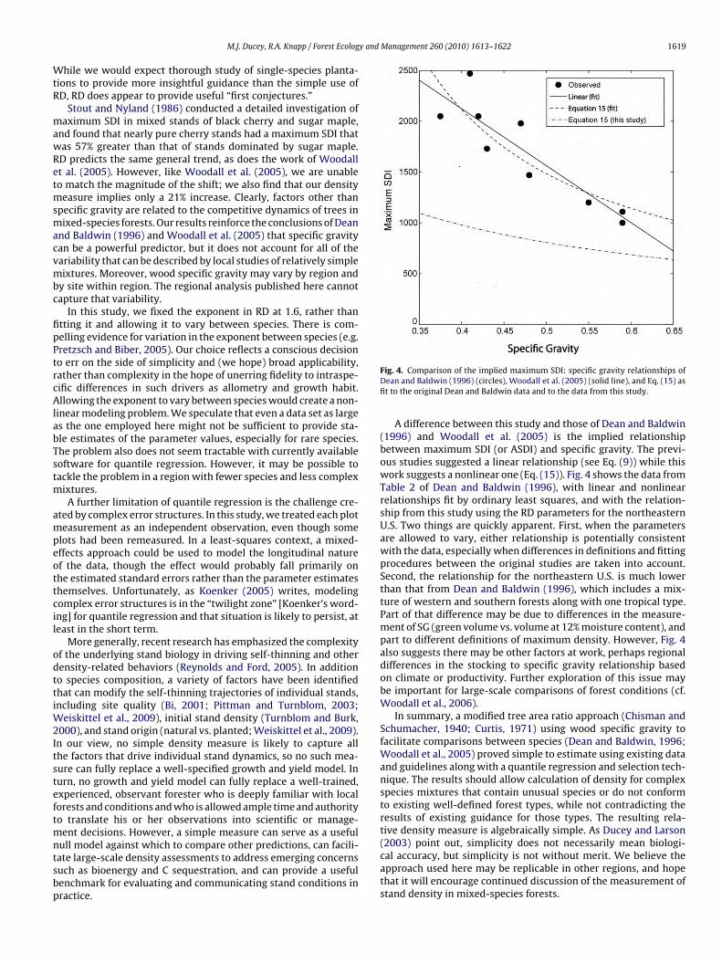
ull model against which to compare other predictions, can facili-ate large-scale density assessments to address emerging concernsuch as bioenergy and C sequestration, and can provide a usefulenchmark for evaluating and communicating stand conditions inractice.

Fig. 4. Comparison of the implied maximum SDI: specific gravity relationships ofDean and Baldwin (1996) (circles), Woodall et al. (2005) (solid line), and Eq. (15) asfit to the original Dean and Baldwin data and to the data from this study.

A difference between this study and those of Dean and Baldwin(1996) and Woodall et al. (2005) is the implied relationshipbetween maximum SDI (or ASDI) and specific gravity. The previ-ous studies suggested a linear relationship (see Eq. (9)) while thiswork suggests a nonlinear one (Eq. (15)). Fig. 4 shows the data fromTable 2 of Dean and Baldwin (1996), with linear and nonlinearrelationships fit by ordinary least squares, and with the relation-ship from this study using the RD parameters for the northeasternU.S. Two things are quickly apparent. First, when the parametersare allowed to vary, either relationship is potentially consistentwith the data, especially when differences in definitions and fittingprocedures between the original studies are taken into account.Second, the relationship for the northeastern U.S. is much lowerthan that from Dean and Baldwin (1996), which includes a mix-ture of western and southern forests along with one tropical type.Part of that difference may be due to differences in the measure-ment of SG (green volume vs. volume at 12% moisture content), andpart to different definitions of maximum density. However, Fig. 4also suggests there may be other factors at work, perhaps regionaldifferences in the stocking to specific gravity relationship basedon climate or productivity. Further exploration of this issue maybe important for large-scale comparisons of forest conditions (cf.Woodall et al., 2006).

In summary, a modified tree area ratio approach (Chisman andSchumacher, 1940; Curtis, 1971) using wood specific gravity tofacilitate comparisons between species (Dean and Baldwin, 1996;Woodall et al., 2005) proved simple to estimate using existing dataand guidelines along with a quantile regression and selection tech-nique. The results should allow calculation of density for complexspecies mixtures that contain unusual species or do not conformto existing well-defined forest types, while not contradicting theresults of existing guidance for those types. The resulting rela-tive density measure is algebraically simple. As Ducey and Larson(2003) point out, simplicity does not necessarily mean biologi-

cal accuracy, but simplicity is not without merit. We believe theapproach used here may be replicable in other regions, and hopethat it will encourage continued discussion of the measurement ofstand density in mixed-species forests.

1 y and Management 260 (2010) 1613–1622

A

esamppA

A

Sw

Appendix A (Continued )

Genus Species 12% specific gravity Source

Magnolia acuminata 0.4800 a

Magnolia fraseri 0.4300 k,m

Malus coronaria 0.6800 l

Malus fusca 0.6800 l

Malus spp. 0.6800 j,m

Morus alba 0.6500 l

Morus rubra 0.6500 b,m

Morus spp. 0.6500 l

Nyssa sylvatica 0.5000 a

Ostrya virginiana 0.7800 b

Oxydendrum arboreum 0.5900 b

Paulownia tomentosa 0.4000 j,m

Picea abies 0.4300 h

Picea glauca 0.4000 a

Picea mariana 0.4600 a

Picea pungens 0.4300 l

Picea rubens 0.4000 a

Picea spp. 0.4300 l

Pinus banksiana 0.4300 a

Pinus nigra 0.4650 l

Pinus pungens 0.4700 d

Pinus resinosa 0.4600 a

Pinus rigida 0.5200 a

Pinus spp. 0.4650 l

Pinus strobus 0.3500 a

Pinus sylvestris 0.4900 h

Platanus occidentalis 0.4900 a

Populus balsamifera 0.3400 a

Populus deltoides 0.4000 a

Populus grandidentata 0.3900 a

Populus heterophylla 0.4000 b

Populus spp. 0.3900 l

Populus tremuloides 0.3800 a

Prunus americana 0.5000 l

Prunus avium 0.5000 l

Prunus pensylvanica 0.3800 k,m

Prunus persica 0.5000 l

Prunus serotina 0.5000 a

Prunus spp. 0.5000 l

Prunus virginiana 0.3800 l

Pseudotsuga menziesii 0.4800 a

Quercus alba 0.6800 a

Quercus bicolor 0.7200 a

Quercus coccinea 0.6700 a

Quercus ellipsoidalis 0.6300 l

Quercus ilicifolia 0.6100 l

Quercus macrocarpa 0.6400 a

Quercus michauxii 0.6700 a

Quercus muehlenbergii 0.6700 l

Quercus palustris 0.6300 a

Quercus prinus 0.6600 a

Quercus rubra 0.6300 a

Quercus spp. 0.6600 l

Quercus stellata 0.6700 a

Quercus velutina 0.6100 a

Robinia pseudoacacia 0.6900 a

Salix alba 0.3900 l

Salix amygdaloides 0.3900 l

Salix bebbiana 0.3900 l

Salix nigra 0.3900 a

Salix spp. 0.3900 l

Sassafras albidum 0.4600 a

Sorbus americana 0.4500 j,m

Sorbus aucuparia 0.4500 j,m

Taxodium distichum 0.4600 a

Thuja occidentalis 0.3100 a

Tilia americana 0.3700 a

Tilia spp. 0.3700 l

Tsuga canadensis 0.4000 a

Tsuga spp. 0.4000 l

Ulmus alata 0.6600 2a

620 M.J. Ducey, R.A. Knapp / Forest Ecolog

cknowledgments

This work was supported under a grant from the National Sci-nce Foundation, “Collaborative Research: The northeastern carbonink: enhanced growth, regrowth, or both?” to M.J. Ducey, withdditional support from the New Hampshire Agricultural Experi-ent Station. The Associate Editor and two anonymous reviewers

rovided valuable comments that greatly improved the paper. Thisaper is scientific contribution number 2437 of the New Hampshiregricultural Experiment Station.

ppendix A.

pecific gravity by species including source information. Specific gravity is based oneight when ovendry and volume when at 12% moisture content.

Genus Species 12% specific gravity Source

Abies balsamea 0.3500 a

Abies spp. 0.3500 l

Acer negundo 0.4440 c

Acer nigrum 0.5700 a

Acer pensylvanicum 0.4600 i

Acer platanoides 0.6200 h

Acer rubrum 0.5400 a

Acer saccharinum 0.4700 a

Acer saccharum 0.6300 a

Acer spicatum 0.4600 l

Acer spp. 0.5050 l

Aesculus glabra 0.3800 b

Aesculus spp. 0.3800 l

Ailanthus altissima 0.5300 e

Alnus glutinosa 0.5100 h

Amelanchier arborea 0.6100 k,m

Amelanchier spp. 0.6100 l

Asimina triloba 0.3969 f

Betula alleghaniensis 0.6200 a

Betula lenta 0.6500 a

Betula nigra 0.6200 l

Betula papyrifera 0.5500 a

Betula populifolia 0.4800 a

Betula spp. 0.6200 l

Carpinus caroliniana 0.7200 b

Carya alba 0.7200 a

Carya cordiformis 0.6600 a

Carya glabra 0.7500 a

Carya laciniosa 0.6900 a

Carya ovata 0.7200 a

Carya spp. 0.7200 l

Castanea dentata 0.4300 a

Catalpa speciosa 0.4000 k,m

Catalpa spp. 0.4000 l

Celtis occidentalis 0.5300 a

Cercis canadensis 0.6300 g

Chamaecyparis thyoides 0.3200 a

Cornus florida 0.7500 b

Crataegus spp. 0.6900 j,m

Fagus grandifolia 0.6400 a

Fraxinus americana 0.6000 a

Fraxinus nigra 0.4900 a

Fraxinus pennsylvanica 0.5600 a

Fraxinus quadrangulata 0.5800 a

Fraxinus spp. 0.5700 l

Gleditsia triacanthos 0.6650 j,m

Ilex opaca 0.6000 b

Juglans cinerea 0.3800 a

Juglans nigra 0.5500 a

Juniperus spp. 0.4700 l

Juniperus virginiana 0.4700 a

Larix laricina 0.5300 a

Larix spp. 0.5300 l

Liquidambar styraciflua 0.5200 a

Liriodendron tulipifera 0.4200 a

Maclura pomifera 0.8400 b

Ulmus americana 0.5000Ulmus rubra 0.5300 a

Ulmus spp. 0.5800 l

Ulmus thomasii 0.6300 a

M.J. Ducey, R.A. Knapp / Forest Ecology and

Appendix A (Continued )

Genus Species 12% specific gravity Source

Unknown broadleaf 0.5121 l

Unknown conifer 0.4450 l

Unknown unknown 0.5279 l

a Forest Products Laboratory (1999).b Panshin and de Zeeuw (1970).c Maeglin and Ohmann (1973).d Burns and Honkala (1990).e Alden (1995).f Nugent and Boniface (2005).g Record and Hess (1943).h Kucera and Naess (1999).i Forest Products Laboratory (2008).j Jenkins et al. (2003).

R

A

A

B

BB

B

C

C

C

C

C

C

C

d

D

D

D

D

F

F

F

G

G

H

J

K

KKK

Weiskittel, A., Gould, P., Temesgen, H., 2009. Sources of variation in the self-

k Markwardt (1930).l Specific gravity based on closely related species.

m Specific gravity converted from green volume to 12% dry.

eferences

lden, H.A., 1995. Hardwoods of North America. USDA For. Serv. Gen. Tech. Rep.FPL-GTR-83, Madison, WI.

ssmann, E., 1970. The Principles of Forest Yield Study. Gardiner, S.H. (trans.) Perg-amon Press, Oxford, UK.

echtold, W.A., Patterson, P.L. (Eds.), 2005. The enhanced forest inventory and anal-ysis program–national sampling design and estimation procedures. USDA For.Serv. Gen. Tech. Rep. SRS-80, Asheville, NC.

i, H., 2001. The self-thinning surface. For. Sci. 47, 361–370.i, H., 2004. Stochastic frontier analysis of a classic self-thinning experiment. Aust.

Ecol. 29, 408–417.urns, R.M., Honkala, B.H. (Tech. coords.), 1990. Silvics of North America: 1. Conifers;

2. Hardwoods. USDA For. Serv. Agriculture Handbook 654, Washington, DC.ade, B.S., Noon, B.R., 2003. A gentle introduction to quantile regression for ecolo-

gists. Front. Ecol. Environ. 1 (8), 412–420.hisman, H.H., Schumacher, F.X., 1940. On the tree – area ratio and certain of its

applications. J. For. 38, 311–317.hui, Y.H., 1993. Evaluation of some structural properties of lumber from Norway

spruce trees grown in the Maritimes. Fredericton, NB: Rep. No. FC9208, WoodScience and Technology Centre, University of New Brunswick.

hui, Y.H., MacKinnon-Peters, G., 1995. Wood properties of exotic larch grown ineastern Canada and north-eastern United States. For. Chron. 71 (5), 639–646.

urtis, R.O., 1970. Stand density measures: an interpretation. For. Sci. 16 (4),403–414.

urtis, R.O., 1971. A tree area power function and related density measures forDouglas-fir. For. Sci. 17 (2), 146–159.

urtis, R.O., Marshall, D.D., 2005. Permanent-plot procedures for silvicultural andyield research. USDA For. Serv., Gen. Tech. Rep. PNW-GTR-634, Portland, Oregon.

e Montigny, L., Nigh, G., 2007. Density frontiers for even-aged Douglas-fir andwestern hemlock stands in coastal British Columbia. For. Sci. 53 (6), 675–682.

ean, T.J., Baldwin Jr., V.C., 1996. The relationship between Reineke’s stand-densityindex and physical stem mechanics. For. Ecol. Manage. 81, 25–34.

ucey, M.J., Larson, B.C., 1997. Thinning decisions using stand density indices: theinfluence of uncertainty. West. J. Appl. For. 12, 89–92.

ucey, M.J., Larson, B.C., 1999. Accounting for bias and variance in nonlinear standdensity indices. For. Sci. 45, 452–457.

ucey, M.J., Larson, B.C., 2003. Is there a correct stand density index? An alternateinterpretation. West. J. Appl. For. 18 (3), 179–184.

orest Products Laboratory, 1999. Wood Handbook: Wood as an Engineering Mate-rial. USDA For. Serv. Gen. Tech. Rep. GTR-113, Madison, WI.

orest Products Laboratory, 2008. Technology transfer fact sheet: acer spp.[online]. Available from http://www2.fpl.fs.fed.us/TechSheets/HardwoodNA/pdf files/acerspeng.pdf (accessed 09.10.08).

rothingham, E.H., 1914. White Pine Under Forest Management. USDA Agric. Bull.,Washington, DC, p. 13.

ilmore, D.W., Briggs, R.D., 2003. A stocking guide for European larch in easternNorth America. North. J. Appl. For. 20 (1), 34–38.

ingrich, S.F., 1967. Measuring and evaluating stocking and stand density in UplandHardwood forests in the Central States. For. Sci. 13, 38–53.

alligan, J.P., Nyland, R.D., 1999. Relative density guide for Norway spruce planta-tions in central New York. North. J. Appl. For. 16 (3), 154–159.

enkins, J.C., Chojnacky, D.C., Heath, L.S., Birdsey, R.A., 2003. Comprehensive databaseof diameter-based biomass regressions for North American tree species. USDAFor. Serv. Northeastern Research Station Gen.Tech. Report NE-319, NewtownSquare, PA.

oenker, R., 2004. Quantreg: An R package for quantile regression and related meth-

ods [online]. Available from http://cran.r-project.org (accessed 19.10.08).

oenker, R., 2005. Quantile Regression. Cambridge University Press, Cambridge, UK.oenker, R., Bassett, G., 1978. Regression quantiles. Econometrika 46, 33–50.ucera, B., Naess, R.M., 1999. Tre – naturens vakreste råstoff. Landbruksforlaget,

Oslo.

Management 260 (2010) 1613–1622 1621

Kurz, W.A., Stinson, G., Rampley, G.J., Dymond, C.C., Neilson, E.T., 2008. Risk of naturaldisturbances makes future contribution of Canada’s forests to the global carboncycle highly uncertain. Proc. Natl. Acad. Sci. 105, 1551–1555.

Leak, W.B., Solomon, D.S., DeBald, P.S., 1987. Silvicultural guide for northernhardwood types in the Northeast (revised). USDA For.Serv. Res. Pap. NE-603,Broomall, PA.

Lindroth, A., Lagergran, F., Grelle, A., Klemedtsson, L., Langvall, O., Weslien, P., Tuulik,J., 2009. Storms can cause Europe-wide reduction in forest carbon sink. GlobalChange Biol. 15, 346–355.

Long, J.N., 1985. A practical approach to density management. For. Chron. 61, 23–27.Long, J.N., 1995. Using Stand Density Index to regulate stocking in uneven-

aged stands. In: Uneven-Aged Management—Opportunities, Constraints, andMethodologies, vol. 56. Montana Forest and Conservation Experiment Station,pp. 110–122.

Long, J.N., Daniel, T.W., 1990. Assessment of growing stock in uneven-aged stands.West. J. Appl. For. 5 (3), 93–96.

Maeglin, R.R., Ohmann, L.F., 1973. Boxelder (Acer negundo): a review and commen-tary. Bull. Torrey Botanical Club 100 (6), 357–363.

Markwardt, L.J., 1930. Comparative strength properties of woods grown in theUnited States. USDA For. Serv. Tech. Bulletin No. 158, Washington, DC,p. 39.

Miles, P.D., Smith, W.B., 2009. Specific gravity and other properties of wood and barkfor 156 tree species found in North America. USDA For. Serv. Res. Note NRS-38,Newtown Square, PA.

Nugent, J., Boniface, J., 2005. Permaculture Plants: A Selection. Chelsea Green Pub-lishing, White River Jct., VT.

Panshin, A.J., de Zeeuw, C., 1970. Textbook of Wood Technology, 3rd ed. McGraw-Hill, New York, New York.

Penner, M., 2008. Yield prediction for mixed species stands in boreal Ontario. For.Chron. 84 (1), 46–52.

Philbrook, J.S., Barrett, J.P., Leak, W.B., 1973. A stocking guide for eastern white pine.USDA For. Serv. Research Note NE-168, Upper Darby, PA.

Pittman, S.D., Turnblom, E.C., 2003. A study of self-thinning using coupled allometricequations: Implications for coastal Douglas-fir stand dynamics. Can. J. For. Res.33, 1661–1669.

Poage, N.J., Marshall, D.D., McClellan, M.H., 2007. Maximum stand-density index of40 western hemlock-sitka spruce stands in southeast Alaska. West. J. Appl. For.22 (2), 99–104.

Pretzsch, H., 2005. Stand density and growth of Norway spruce (Picea abies (L.) Karst.)and European beech (Fagus sylvatica L.): evidence from long-term experimentalplots. Eur. J. For. Res. 124 (3), 193–205.

Pretzsch, H., Biber, P., 2005. A re-evaluation of Reineke’s rule and stand density index.For. Sci. 51 (4), 304–319.

Puettmann, K.J., Hibbs, D.E., Hann, D.W., 1992. The dynamics of mixed stands of Alnusrubra and Pseudotsuga menziesii: extension of size-density analysis to speciesmixture. J. Ecol. 80, 449–458.

R Development Core Team, 2008. R: A language and environment for statisti-cal computing, version 2.7.2 (2008-08-25). Vienna, Austria: The R Foundationfor Statistical Computing. ISBN 3-900051-07-0. Available from http://www.r-project.org/ (accessed 19.10.08).

Record, S.J., Hess, R.W., 1943. Timbers of the New World. Yale University Press, NewHaven, CT.

Reineke, L.H., 1933. Perfecting a stand-density index for even-aged forests. J. Agric.Res. 46, 627–638.

Reynolds, J.H., Ford, E.D., 2005. Improving competition representation in theoreticalmodels of self-thinning: a critical review. J. Ecol. 93, 362–372.

Scharf, F.S., Juanes, F., Sutherland, M., 1998. Inferring ecological relationships fromthe edges of scatter diagrams: comparison of regression techniques. Ecology 79(2), 448–460.

Shaw, J.D., 2000. Application of stand density index to irregularly structured stands.West. J. Appl. For. 15 (1), 40–42.

Shaw, J.D., 2006. Reineke’s stand density index: where do we go from here? In:Proceedings: Society of American Foresters 2005 National Convention, Octo-ber 19–23, 2005, Ft. Worth, TX [published on CD-ROM]. Society of AmericanForesters, Bethesda, MD.

Solomon, D.S., Zhang, L., 2002. Maximum size-density relationships for mixed soft-woods in the northeastern USA. For. Ecol. Manage. 155, 163–170.

Stout, S.L., Nyland, R.D., 1986. Role of species composition in relative density mea-surement in Allegheny hardwoods. Can. J. For. Res. 16, 574–579.

Stout, S.L., Marquis, D.A., Ernst, R.L., 1987. A relative density measure for mixed-species stands. J. For. 7, 45–47.

Swift, E., Penner, M., Gagnon, R., Knox, J.A., 2007. Stand density management dia-gram for spruce-balsam fir mixtures in New Brunswick. For. Chron. 83 (2), 187–197.

Turnblom, E.C., Burk, T.E., 2000. Modeling self-thinning of unthinned Lake States redpine stands using nonlinear simultaneous differential equations. Can. J. For. Res.30, 1410–1418.

VanderSchaaf, C.L., Burkhart, H.E., 2007. Comparison of methods to estimateReineke’s maximum size-density relationship species boundary slope. For. Sci.53 (3), 435–442.

thinning line for three species of varying shade tolerance. For. Sci. 55 (1),84–93.

Woodall, C.W., Miles, P.D., Vissage, J.S., 2005. Determining maximum stand densityindex in mixed species stands for strategic-scale stocking assessments. For. Ecol.Manage. 216, 367–377.

1 y and Management 260 (2010) 1613–1622

W

Y

622 M.J. Ducey, R.A. Knapp / Forest Ecolog

oodall, C.W., Perry, C.H., Miles, P.D., 2006. The relative density of forests in theUnited States. For. Ecol. Manage. 226, 368–372.

oda, K., Kira, T., Ogawa, H., Hozumi, K., 1963. Intraspecific competition amonghigher plants. XI. Self-thinning in overcrowded pure stands under cultivatedand natural conditions. J. Biol. Osaka City Univ. 14, 107–129.

Zeide, B., 2005. How to measure stand density. Trees 19, 1–14.Zhang, L., Bi, H., Gove, J.H., Heath, L.S., 2005. A comparison of alternative meth-

ods for estimating the self-thinning boundary line. Can. J. For. Res. 35,1507–1514.