A stability analysis of non-time-periodic perturbations of buoyancy-induced flows in pure water near...

J. Fluid Mwh. (1986), VOZ. 163, p ~ . 1-20

Printed in Great Britain 1

A stability analysis of non-time-periodic perturbations of buoyancy-induced flows in pure

water near 4 "C

By I. M. EL-HENAWY, Department of Mathematics, Mansoora, University, Mansoora, Egypt

B. D. HASSARD AND N. D. KAZARINOFF Department of Mathematics, State University of New York at Buffalo, N.Y. 14214 U.S.A.

(Received 1 February 1984 and in revised form 24 June 1985)

A new approach to determine stability of multiple steady-state similarity solutions corresponding to laminar flows is introduced and applied to laminar flows in cold, pure water at temperature T, "C (near 4 "C) adjacent to a vertical, isothermal, plane surface at temperature T, "C when 0 < R = (4-T,)/(q-Tm) < 0.5, the region of buoyancy-force reversals. The results show that the steady-state similarity solutions recently found in this region by El-Henawy et al. (1982) are unstable, and thus should not be observed experimentally; while those solutions found earlier by Carey, Gebhart & Mollendorf(l980) may be stable. No unstable modes corresponding to their solutions were found. Some flows for R in the range of strong buoyancy-force reversals, 0.14 < R < 0.32 at Prandtl number Pr = 11.6, have been observed, for example at R = 0.143,0.254 and 0.317 by Carey & Gebhart (1981) and Wilson & Vyas (1979). The latter found time-varying flows in this region of strongest flow reversals.

The advantages of the method introduced are reduction of mathematical short- comings of the traditional approach and relative ease of numerical calculation of the real eigenvalues and eigenfunctions. The disadvantage is that information on downstream, selective frequency, exponential growth of amplitude is lost. The theory presented may be regarded as an asymptotic limit of the standard hydrodynamic theory as the frequency of perturbations approaches zero.

1. Introduction The stability characteristics of boundary-layer flows in pure or saline water close to

its temperature of maximum density T, "C are of particular interest, for then the local temperature T "C of the water relative to T, strongly influences the velocity and temperature profiles of the steady-state similarity solutions and the experimentally observed flows; see Wilson & Vyas (1979), Carey & Gebhart (1981), Sammakia (1981) and El-Henawy et al. (1982), and figure 1. For the similarity solutions corresponding to the laminar flow of cold, pure water adjacent to an isothermal, semi-infinite flat plate (seefigure2) thisoccursforR = (Tm-T,)/(T,-Tm) close toeither0.151 or0.292. For T, = 0 "C and T, = 4.029325 "C this means that the initial temperature of still, cold, pure water is close to either 4.7460 "C or 5.6911 "C. Moreover, for R in each of the ranges (0.15148, 0.15180) and (0.29181, 0.45402), corresponding to T, in the ranges (4.74865 "C, 4.75044 "C) and (5.6886 "C, 7.3800 "C), multiple solutions of the similarity equations were found by El-Henawy et al. (1982). Some pairs of these

2

P c

c I

L

I . M . El-Henawy, B. D . Hassard and N . D . Kazarimff

T

1 T T

RQURE 1. The effect of specified temperatures T, and T, on R, on the buoyancy force B(T) and on flow direction. T,, T, and T, are the temperatures of the isothermal plate, of the ambient water, and at which water has maximum density. The subscripted variables p are the corresponding densities. (a) B > 0, R < 0, and the flow is up; (b) B < 0, R > 0, and the flow is down; (c) B < 0, R = +, and the flow is down; and (a) B > 0, R = 0, and the flow is up.

-3 0

Y

Y

(4 (b)

FIGURE 2. The coordinate systems: (a) upflow, (a) downflow.

Stability of perturbations of buoyancy-induced flows 3

1 '

0.151 80 0.291 80 R

0.15180 0.291 80 R

FIGURE 3. Variation of P( co) and - W(0) with R (base flows).

existing at the same R > 0.292 have distinctly different velocity and temperature profiles, including vastly different heat-transfer rates at the vertical surface. If flows with dramatically low heat-transfer rates are observable in the laboratory, then it might be possible to take advantage of the conditions that cause them in technological applications. Both Wilson t Vyas (1979) and Carey & Gebhart (1981) observed flows in the range (5.69 "C, 7.38 "C), for example at 5.9 "C. Wilson & Vyas wrote ' It is noted that oscillations become appreciable exactly within the dual flow regime. . . '. Carey & Gebhart found the flow to depart from numerical predictions at 4.7 "C except close to the ice wall.

In view of the uncertainties about the nature of the flows of pure water in the region of strong buoyancy-force reversals (4.7-7.38 "C) and the numerical discovery of multiple steady-state solutions in this range, both more experimental work and analysis are needed. The stability of the multiple steady-state solutions, which has not been studied previously, and the implications the results have for actual flows are the object of our investigation. As will be seen, the approach we follow is widely applicable to problems for which multiple steady-state solutions are found. In brief, our results indicate that the solutions with strong velocity reversals and very low heat-transfer rates are not stable in time to small perturbations. Our results for the stability of laminar, steady-state flows of cold, pure water adjacent to a vertical, semi-infinite, flat, isothermal surface (hereafter called Problem S) are best described in terms of bifurcation diagrams for the two known families of steady-state solutions ( F ( T ) , @ ( ~ ) ) of (1.7) below, one existing for R < 0.1518 (largely upflow), the other existing for R > 0.2918 (largely downflow), see figure 3 (a , b). We show in 52 that the

4 I . M . El-Henawy, B. D. Hassard and N . D . Kazarinoff

steady-state solutions, which exist for R < 0.1518 and which correspond to points (R, F(co)) in the bifurcation diagram 3(a) with F(co) below its value (approximately 0.045) at N,, are unstable (at least one eigenvalue of the associated linear system (1.9) below is positive). We believe that those solutions corresponding to points with F( co) above its value at N , may be stable (we found no eigenvalue h that is positive there). We also show in $2 that the steady-state solutions, which exist for R > 0.291 and which correspond to points (R, - Q'(0)) in the bifurcation diagram figure 3 (b) with -@' (O) below its value (approximately 0.493) at N , are unstable (we found one positive A) , and those with @'(O) above its value at N may be stable (we found no positive h there).

For the family of solutions that exists for R < 0.16, we found three eigenvalues h = A,(R, F( 0 0 ) ) with eigenvectors K(q), # l ( q ) ) (i = 1 , 2, 3). For i = 1 and 2, A,(R, F( co)) changes its algebraic sign at the nose Ni in figure 3 (a). We did not find a third nose N , at which h,(R, F(oo)) changes its algebraic sign, but we conjecture that such a nose exists.

Among the many previous experimental or numerical studies of Problem S (including various fluids and either a uniform flux or isothermal boundary condition) are those by Nachtsheim (1963), Polymeropoulos & Gebhart (1967), Knowles & Gebhart (1968), Dring & Gebhart (1968, 1969), Gill & Davey (1969), Vliet & Liu (1969), Jaluria & Gebhart (1974), Gebhart (1979), Qureshi (1980), Higgins (1981), and (a contemporary study) Hwang, Kazarinoff & Mollendorf (1984). Nachtsheim made a thorough and skilful analysis of the isothermal-plate problem in the Boussinesq case (buoyancy force linear in 7'). The experimental results of Polymeropoulos & Gebhart confirmed Nachtsheim's numerical results within reasonable limits. Qureshi was the first to compute neutral-stability curves using the nonlinear buoyancy-force function of Gebhart & Mollendorf (1977). He did this for the no-flux boundary condition for saline water at R = 0 and compared the results with experimental data. Higgins computed the neutral-stability curve and contours of constant amplification a t R = 0.4 for Problem S. She also verified, within rough limits, her theoretical results with experiments. Hwang et al. determined neutral-stability curves of the same problem.for 0.291 81 < R < 0.34 and found that, as one descends to below the nose N in figure 3 ( b ) , the corresponding solutions are amplified ever closer to the leading edge of the plate. All the numerical analyses cited above have implemented what we call here the traditional or conventional approach t o hydrodynamic stability (Drazin & Reid 1981 ; Lin 1955).

Our approach is distinctly different from the conventional one, as will be seen below. The Problem S studied here is the stability of steady-state, similarity solutions of the Navier-Stokes-energy system

p(us+vy) = 0, (1.la)

1 Ut + UU, + vuY = - -pz + u AU + B( T),

P ( l . l b )

( l . l c )

T,+uT,+vT, = &AT, ( l . ld )

u ( z , O , t ) =v(z ,O, t )=T(z ,O, t ) -T,=T(x,co, t ) -T, =u(x,co, t )=O, ( l . l e )

where T is the temperature at (x, y, t ) , B(T) denotes buoyancy force, x and y are coordinates respectively parallel and perpendicular to the vertical, isothermal surface y = 0 (see figure 2), t is time, u and v are respectively the vertical and horizontal

1

P vt +UV,+VV~ = --py + v Av,


components of fluid velocity at (x, y, t ) , p is the motion pressure at (x, y, t ) and p is the (constant) density of pure water at temperature T.

The buoyancy force B(T) has been fitted to data by Gebhart & Mollendorf (1977) to within 3.5 p.p.m. accuracy for pure water. In terms of

their formulation is

where for pure water at 1 bar

q = 1.894816, a = (9.297 173 x 10+ O C ) * and T, = 4.029325 "C.

Also, g = 9.81 m/s2, and v 'v 1.67 x mz/s. In (1.3) the + sign is used for base (steady-state) flows that are largely upflow (see figures l a and 2a) which occur for R < 0.151 80, and the - sign is used for base flows that are largely downflow (see figures 1 b and 2b) which occur for R 2 0.291 81.

We begin our analysis of Problem S for (l . l) , with B(T) as in (1.23), by making a similarity transformation from (x, y, t) to (7, 7 ) defined by

where C, is a constant to be determined later, which will non-dimensionalize 7 , and the Grashof number G is defined to be

G = 4[f &(x, T,)]i

(1.5) with

We also choose a stream function $ so that, as usual, u = $z and v = - $.,. In addition to $, given by (1.2), we define new dependent variables f and P in terms of (7, 7 ) by

(1.6)

We rewrite (1.1) in terms of these new dependent and independent variables and in writing each equation we neglect terms of order GW2 compared with other terms in the same equation, exactly as was done by El-Henawy et al. (1982). In the traditional approach the parallel-flow hypothesis is used, and terms of order 1/G are neglected; see Hieber & Gebhart (1971). The truncated similarity equations, which are derived from (1.1) using (1.2)-( 1.5), are :

f q T + 2 f ; - 3 f f , q + 2 7 ~ q q f T - f q f q T > =fq,,+{I$-RIQ-IRIq), ( 1 . 7 ~ )

G(z, T,) = - 7 ~ ~ ccg IT,-T,I*.

$(x, y, t) = .Gf(r, 71, P(7 ,7 ) = p (FGY - P(X, y, t) .

f T - 7 f , T - 27fT7 + 9ff, - 7f; - 37ff,, - 47fTf7 - 47YTT - 277vq7 f q - fqq f T >

= - p, +7f,,q - f q l r + 6 7 f f ~ - 4 7 Y T f q T + 2 f , q T , (1-7b)

Pr( - 3f$, + $7 - 27 {$Tf7) - f T $qH = $?/q, ( 1 . 7 ~ )

with boundary conditions

f ( 0 , T ) =f,(0,7) = $ ( O , T ) - l = 0, f,(m,7) = $(m,7) = 0, P(m,7) = 0. ( l .7d)

In ( 1 . 7 ~ ) Pr = v/& is the Prandtl number, chosen to be 11.6 throughout. We have also chosen C , = t [gcz 1%- T,l*]k This non-dimensionalizes 7 and makes the coefficient

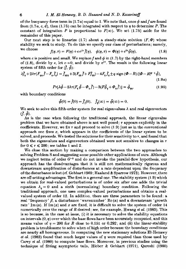
6 I . M . E l -Henaq , B. D . Hassurd and N . D . Kazarinoff

of the buoyancy-force term in ( 1 . 7 ~ ) equal to 1. We note that, once $ and f are found from (1.7a, c, d), then (1.7b) can be integrated with respect to 7 to determine P. The constant of integration P is proportional to F(m). We set (1.7b) aside for the remainder of this paper.

Our next step is to linearize (1.7) about a steady-state solution (F, @) whose stability we seek to study. To do this we specify our class of perturbations; namely, we choose

where 8 is positive and small. We replacef and $ in (1.7) by the right-hand members of (1.8), divide by 8, let e+O, and divide by eh7. The result is the following linear system of fifth order for $, 6) :

f ( T ? 7 ) = P(7) +8eA7.7((r), $(T> 7 ) = @(7) +k+6(7), (1.8)

~J,+2W$,P--,xJ =Jqtlr+3(F,,J+FJ,,,)-4F,~,f~ sign (@-R) (l@-Rlq-16)9 (1.9a)

Pr[h6-2h7(F,6-@,J)--(F6,+@,3)1= 6,,,, (1.9b)

with boundary conditions

6(0) =.m = J 7 ( O ) , J , ( 4 = 6 ( 4 = 0.

We seek to solve this fifth-order system for real eigenvalues h and real eigenvectors

As is the case when following the traditional approach, the linear eigenvalue problem that we have obtained above is not well posed; 7 appears explicitly in the coefficients. However, we fix 7 and proceed to solve (1.9) just as in the conventional approach one fixes 5, which appears in the coefficients of the linear system to be solved, and proceeds. We tested the solutions for their sensitivity to 7 , and found that both the eigenvalues and eigenvectors obtained were not sensitive to changes in 7

for 0 < 7 < 200; see tables 1 and 2. We close this section by making a comparison between the two approaches to

solving Problem S and suggesting some possible other applications of ours. Although we neglect terms of order G-2 and do not invoke the parallel-flow hypothesis, our approach has the disadvantages that it is still not mathematically rigorous and downstream amplification of disturbances at a rate dependent upon the frequency ofthe disturbance is lost (cf. Gebhart 1969; Haaland & Sparrow 1973). However, there are off-setting advantages. The first is a general one. The stability system (1.9) which we obtain for real-valued perturbations is of order six after one adds the trivial equation A, = 0 and a sixth (normalizing) boundary condition. Following the traditional approach, one uses complex-valued perturbations and obtains a real- valued system of order 12. In addition, there are three parameters to be found: a real ' frequency ' B, a disturbance ' wavenumber ' Re (a) and a downstream ' growth rate' Im (a). If Im(a) and z are fixed, i t is difficult to solve the system of order 14 numerically over the range of R desired; see, for example, Hwang et al. (1985). This is so because, in the case at issue, (i) i t is necessary to solve the stability equations on intervals ( 0 , ~ ) over which the base flows have been accurately computed, and this means value of 7 = 200 for R close to 0.151 or 0.292; and (ii) the linear-stability problem is troublesome to solve when of high order because the boundary conditions are nearly all homogeneous. In computing the new stationary solutions El-Henawy et al. (1982) found that much larger values of 7 were required than those used by Carey et al. (1980) to compute base flows. Moreover, in previous studies using the technique of fitting asymptotic tails, Hieber t Gebhart (1971), Qureshi (1980)

(.L $1.

Stability of perturbations of buoyancy-induced $ows 7

7

0 0.5 1 .o 2.0 5.0

10.0 20.0 50.0

100.0 150.0 200.0

A,(0.151 775, 0.050)

-0.321907 x lo-' -0.319652 x lo-' -0.317417 X lo-' -0.313005 x lo-' -0.300457 x lo-' -0.281576 X lo-' -0.249280 x lo-* -0.183688 x lo-' -0.126613 x lo-* -0.972309 x lo-' -0.777365 x

Al(O. 151 788, 0.042)

0.232 845 x 0.230691 x 0.228580 x 10-2 0.224476 x lo-' 0.213045 x 0.196477 x 0.170 252 x 0.122 124 x lo-* 0.834 114 x lop3 0.714213 x 0.512604 x

TABLE 1. The dependence of the eigenvalue A,, evaluated at R = 0.151775, F ( w ) = 0.05, upon 7

(column 2), and the dependence of the same eigenvalue A, evaluated at F ( w ) = 0.042, R = 0.151 788 upon 7 (column 3). All computations done at T~ = 200.0.

7 ~(0.291829, 0.5) ~(0.291897, 0.48)

0 0.5 1 .o 5.0

10.0 50.0

100.0 200.0

-0.385432 x to-' -0.386239 x lo-' -0.388972 x lo-' -0.396233 x lo-' -0.409314 x lo-' -0.423932 x lo-' -0.439322 x lo-' -0.401 239 x lo-'

0.695293 x lo-' 0.703256 x lo-' 0.720093 x lo-' 0.756245 x lo-' 0.758521 x 0.762839 x lo-' 0.771 003 x lo-* 0.763994 x lo-'

TABLE 2. The variation of y(R, - @ ' ( O ) ) with 7 for two points (R, -@'(O)) near to N in figure 3

and Higgins (1981) integrated in from q with 7 = 14 or 20 (Hieber & Gebhart), q = 8 (Qureshi), and 7 = 3 or 5 (Higgins). Even if one employs asymptotic tails, substantially larger values of 7 are required. Our use of real-valued perturbations means, not only in the present application but in general, a gain by a factor of two in the order of the linear-stability system to be solved over the order of the linear system for the real and imaginary parts of complex-valued perturbations used in the traditional approach.

A second advantage of the present analysis over the traditional one is specific to the application at hand. If one uses the buoyancy-force function B(T) defined in (1.3), eliminates p from (1.1) by taking the curl of (1.1 b , c ) , and then linearizes about a base flow, the function B(T) is differentiated twice. But the exponent q in (1.2) lies between 1 and 2. Thus there is a singularity in the coefficients of the linear-stability system obtained at a value of 7 for which @ ( v ) = R, and since @ decreases monotonically from 1 to 0 on ( 0 , ~ ) such a value of R exists for every R within (0.0, 0.5), the range of greatest interest. The present approach does not create such a singularity.

In summary, we believe that our approach has advantages that compensate for its disadvantages, both for the present application and potentially in other laminar- fluid-flow problems where multiple steady-state solutions have been found ; for example, by Gebhart et al. (1983) for a problem involving porous media, by Brady & Acrivos (1981, 1982), Brady (1984), Durofsky & Brady (1984) for flow in an accelerating pipe, and by Gill et al. (1985a,b) for surface-tension-driven flow of

8 I . M . El-Henawy, B. D. Hassard and N . D . Kazarinoff

vm A1(0.151 775. 0.050) A,(0.151788, 0.042)

40.0 -0.258934 x lo-' 0.21 1941 x lo-' 60.0 -0.261 210 X lo-' 0.208 135 x lo-'

100.0 -0.269591 X lo-' 0.204 128 x lo-' 150.0 -0.276518 x lo-' 0.200 158 x lo-' 200.0 -0.281 576 X lo-' 0.196470 x lo-'

TABLE 3. The dependence of the eigenvalue A , , evaluated at P( a) = 0.050, R = 0.151 775, upon 7, (column 21, and the dependence of the same eigenvalue A,, evaluated at F ( a ) = 0.042, R = 0.151 788, upon qrn (column 3). All computations done at T = 10.0.

low-Prandtl-number fluids in various geometries. The method presented here can help to select which of multiple steady states is stable to time-dependent perturbations. The bifurcation diagrams that describe multiple steady-state solutions typically have points of vertical tangency. Usually, where vertical tangencies are found in bifurcation diagrams for time-independent solutions, the real part of one eigenvalue changes sign as one follows the diagram through the point of vertical tangency. Contemporary bifurcation theory is replete with examples : see for example, Iooss & Joseph (1980) or Hassard, Kazarinoff & Wan (1981).

2. Stability analysis and results We solved the linear system (1.9) together with the suspended trivial equation

A, = 0 and a sixth boundary condition, specifying either f( 00) = 1 for R < 0.151 80 or $ ( O ) = 1 for R 2 0.291 81. The eigenvalue problems thus obtained were solved, given (R, f(00)) or (R, $&O)), on a finite interval with boundary conditions a t cx) imposed at 7 = 200. We chose 7 = 200 since this is the value that is acceptable for the steady-state solutions whose stability is the issue.

The presence of 7 in the coefficients of the system (1.9) shows that the formal assumption (1.8) is not mathematically correct. Nevertheless, we have solved the eigenvalue problem (1.9) numerically, for fixed values of 7. We used two totally different computer codes. The first is COLSYS, collocation two-point-boundary-value- problem solver; see Ascher, Christiansen & Russell (1978). The second is BOUNDS, a multiple shooting, two-point-boundary-value-problem solver ; see Deuflhard (1980), Deuflhard & Bader (1982), and Bulirsch & Stoer (1966). COLSYS was chosen for its reliability and, in particular, because aftcr solving the steady-state problem for F and @ using COLSYS, one can store the spline nodes and coefficients, and subsequently evaluate F, @ and their derivatives in a COLSYS subroutine APPSLN for use in solving (1.9). BOUNDS does not have this ability, since output from BOUNDS consists only of values of solution components a t user-specified nodes. Using COLSYS to solve the eigenvalue problem for fixed 7 was straightforward. To use BOUNDS we included the subroutine APPSLN from COLSYS in our main driving program to give values of the coefficients in (1.9) at points called by BOUNDS. Both BOUNDS and COLSYS were run in FORTRAN 4.8 on a CYBER 174. The approximate run time per solution was 40 s for each code.

Stability of perturbations of buoyancy-induced flows

0.07

0.06

0.05

F(m)

0.04

0.03

0.02

0.01

0.1514 0.1515 0.1516 0.1517 0.1518

R

9

0.25 0.30 0.35 0.40 0.45 0.50

R

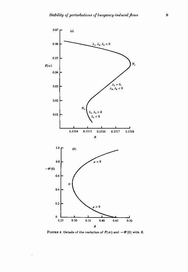
FIGURE 4. Details of the variation of P( 00) and - W(0) with R.

10 1. M . El-Henawy, B . D . Hassard and N . D. Kazarinoff

0.012 -

0.008 -

0.004 ~

c 0 -

-0.004 -

-0.008 t

0.006

(c ) 0.012 - (d )

0.008 -

0.004 - P

0 -

-0.004 -

1 -0.008 - i

0.003

A

0

-0.003

- 0.006

0.006

0.003

A

0

-0.003

-0.006 0.15144 0.15152 0.15160 0.15168 0.15176 0.15184 0.008 0.016 0.024 0.032 0.040 0.048 0.056

R F ( m )

3. Bifurcation diagrams and stability For R in [0.151486,0.151801] we found and computed three eigenvalues

h = h d ( R , F ( ~ ) , 7 ) (i = 1, 2, 3)

and corresponding eigenvectors

@A% 7)3 4c(.rr,7HT. Since 7 appears explicitly in the coefficients of the linear system (1.9), the eigenvalues and eigenvectors obtained depend parametrically upon 7. However, this dependence is weak; see tables 1 and 2. In fact, the dependence upon 7 becomes negligible in the neighbourhood of a 'nose ' a t which h = 0, since 7 appears in the governing equations (1.9) only in the combination h7. This supports the formal assumption (1.8). In

Stability of perturbations of buoyancy-induced flows 1 1

@ and

@' and

+ : ; : ; : :+

-0.2 I 1 I I I I I 1 1.0 2.0 3.0 4.0 5.0 6.0 7.0 8.0

7

0.2

0

-0.2

& - 0.4

-0.6

-0.8

1 (b)

0 1.0 2.0 3.0 4.0 5.0 6.0 7.0 8.0 t

-

0.8 - F a n d j

t I I I I 1 I I 1 I 1 0 5.0 10.0 15.0 20.0 25.0 30.0 35.0 40.0 45.0 50.0

t FIGURE 6. For caption see p. 12.

12 I . M . El-Henawy, B. D . Hassard and N . D . Kazarinoff

-0.2 ! 1 I I I 1 I I I I 1 0 5.0 10.0 15.0 20.0 25.0 30.0 35.0 40.0 45.0 50.0

9

FIGURE 6. Base flows (F, @) and corresponding eigenvector componenJs (1st mode; curves marked with crosses) (f, 6) a t R = 0.151 775 and F ( c o ) = 0.050: (a) @ and 4, (b) @’ and $’, (c) F andf, (d) F’ a n d y .

-0.2 A I

0 1.0 2.0 3.0 4.0 5.0 6.0 7.0 8.0

9

+

0 1.0 2.0 3.0 4.0 5.0 6.0 7.0 8.0 9

FIGURE 7(a) and ( b ) . For caption see opposite.


’.O - (c)

- -x

0.8 -

0.6 - F and j

0.4 -

0 I5 30 45 60 75 90 105 I20 135 150 165 180 7

F and?

- 1 x

-0.04 i 0 15 30 45 60 75 90 105 120 135 150 165 180

7

FIGURE 7. Base flews ( F , @) and corresponding eigenvector components (2nd mode; curves marked with crosses) (f, q5) at R = 0.151486, P(c0) = 0.015: (a) @ and 4, ( b ) @’ and $, (c) F and!, ( d ) F and T. addition to the dependence upon r described above, we also tested A, for its response to changes in qffl for qm in the interval [40.0, 200.01 (see table 3), for 7 = 10.0. We did this for two points (R , F(ao)) close to the nose N, , namely (0.151 775, 0.050) and (0.151788, 0.042). The results show that A, is reasonably insensitive to changes in qffl. The corresponding eigenvectors change only in the fifth decimal place for these changes in 7 and qm. For R > 0.29, we found and computed just one eigenvalue p ( R , - @’(O), 7 ) for points (R, - @’(O)) in the bifurcation diagram 4 ( b ) . We tested for its sensitivity to 7 (see table 2). The dependence on 7 is weak, as expected near a ‘nose’. We also found p to be reasonably insensitive to changes in qffl (table not shown). I n the following computations, the values r = 10.0 and q = 200.0 were used. For brevity, we shall not show 7 as a parameter in subsequent formulae involving eigenvalues and/or eigenvectors.

The eigenvalues hi (i = 1,2 ,3) have the following properties. First, A,(R, F( 00)) = 0 a t (R, F( 0 0 ) ) N (0.151 801,0.0455), the nose N , in the bifurcation diagram figure 3 (a ) ; A,(R, F(oo)) < 0 for F(m) greater than its value a t this nose; and A,(R, F ( o o ) ) > 0 for F ( w ) less than its value at this nose; see figures 4(a), 5(a , b ) . Similarly, A,@, F(oo)) = 0 a t ( R , F(co)) N (0.151 486, 0.014), the nose N , in the bifurcation diagram figure 3(a); A,(R,F(co)) < 0 for F(co) greater than its value at N , ; and A,(R,F(co)) > 0

14 I . M . El-Henuwy, B. D. Hassard and N . D . Kazarinoff

1 .o

0.8

0.6

@ and 4 0.4

0.2

0

-0.2 0 1.0 2.0 3.0 4.0 5.0 6.0 7.0 8.0

I I

m : : : : : : : : : : : l -

@' and &

1

0 1.0 2.0 3.0 4.0 5.0 6.0 7.0 8.0 11

1 .o

0.8

0.6

0.4

F and] 0.2

0

-0.2

-0.4 0 I5 30 45 60 75 90 105 120 135 150 165 180

11 FIGURE S(a-r). For caption see opposite.


F and?

t

0 15 30 45 60 75 90 105 120 135 150 1

. . . - FIGURE 8. Base flows (F, @) and corresponding eigenvector com onents (3rd mode; curves marked with crosses) (3, $) at R = 0.151735, F(co) = 0.037: (a) @ and 8, (b ) @' and q?, (c) F and!, ( d ) P, andy.

for F ( m ) less than its value a t N , ; see figures 4(a), 5(a, b) . The third eigenvalue A, (R, F(co)) is negative and increasing as F(m) decreases from 0.050 to 0.009; see figures 4(a), 5(a, b). We conjecture (based upon figure 5 b ) that there exists a third nose N3 at a point (R, F( 0 0 ) ) with P(m) < 0.009 at which A,(R, F ( m ) ) = 0; but we were not able to find such a nose within what we judged to be a reasonable amount of computing effort.

We conjecture that there are infinitely many noses existing for R < 0.16 in the complete bifurcation diagram that is partially given in figure 4(a) and that corresponding to the ith nose is an eigenvalue A,(R, p(00)) that vanishes at the ith nose, is negative for values of F(w) greater than its value at this nose, and is positive for all F ( w ) 2 0 less than the value of F ( m ) at this nose. We also conjecture that all members of the family of steady-state solutions with F( 00) greater than its value at the first nose N , are stable and all others with values of F ( m ) less than its value at N , are unstable. In stating that a steady-state solution is stable we mean that small perturbations of the form (1.8) all decay exponentially to 0 as t ++ 00 for each fixed (2, y ) , and in stating that a steady-state solution is unstable we mean that the absolute value of some perturbations of the form (1.8) grows exponentially to + 00 as t + + 00

for almost all fixed (z, y ) . The eigenvalue p ( R , - @'(O) ) changes sign at the unique nose N of the bifurcation

diagram 4 ( b ) . The nose lies at approximately (0.291808, 0.493): p < 0 for -@' (O) greater than its value at this nose, and p > 0 for -@'(O) less than its value at N; see figures 5(c ,d ) . For -@'(O) greater than its value at the nose, we believe the steady-state solutions are stable, but lose stability as -@'(O) is decreased beyond 0.493.

To show how the eigenvector components vary with R and how they compare with the corresponding base-flow-solution components, we present figures 6-9. Figures 6-8 cover the situation R < 0.16 (largely upflow), while figure 9 is for R > 0.29 (largely downflow). Figure 6 shows a solution for R = 0.151 75, and F ( m ) = 0.050, slightly below the first nose seen in figure 3 (a). The first eigenmode is shown with the base-flow solution because this mode causes the base flow to lose stability as P(co) decreases from above to below the first nose. The corresponding plots (not shown) for R = 0.151 75, but F ( w ) = 0.048, slightly below the nose, are virtually identical.

16 I . M . El-Henawy, B. I ) . Hassard and N . D . Kazarinoff

# and

1.1

0.7

0.3

4' -0.1

-0.5

-0.9 0 1.0 2.0 3.0 4.0 5.0 6.0 7.0 8.0

II

FIGURE 9(a) and ( b ) . For caption see opposite.

Analogous statements hold a t the other noses. Figure 7 represents a solution for R = 0.151 1486 and F ( a ) = 0.015, slightly above the second nose seen in figure 3(a) . The second eigenmode is shown with the base-flow solution since the eigenvalue A, becomes positive as F(co) decreases past the second nose. Figure 8 shows the base solution and the corresponding third eigenmode for a value F( CO) below the first nose but above the second nose. At this value of F ( c o ) , A, >0 , A, < 0 and A, < 0. A, remains negative as F( CO) is decreased past the second nose. We conjecture that A, becomes positive past a conjectured third nose. Figure 9 represents a solution on the upper side of the nose in figure 3 ( b ) . The eigenmode shown with the base-flow solutions causes the loss of stability as - @'(O) is decreased from above to below the nose.


0.15

0.10

0.05

F and f 0

-0.05

-0.10

-0.15

0 2.0 4.0 6.0 8.0 10.0 12.0 14.0 16.0 18.0 20.0 t

0.10 - (d )

0.05 -

0 4 - ..

F and?

-0.05

-0.10 -

-0.15 -I I 1

0 2.0 4.0 6.0 8.0 10.0 12.0 14.0 16.0 18.0 20.0 t

FIQURE 9. Base flows ( F , @) and corresponding eigenvector components (unique mode found; curves marked with crosses) (f, 6) at R = 0.291878, -@’ (0) = 0.505: (a) @ and 4, ( b ) @’ and 8, (c) F andf, ( d ) F’ and?.

4. Discussion We first discuss the behaviour of our perturbations

in terms of x , y and t and the vertical and horizontal components of the perturbed velocity cfi(x, y , t ) and cG(z, y, t ) and the perturbed temperature @(x, y , t ) . These are

18

and

Since G = const. x xi, for fixed t , .ii grows downstream as xi along streamlines 7 = const., and v’ decays like x-i. Our allowed perturbations are not time-periodic, and the observed limiting behaviour of the conventionally studied ‘ time-periodic ’ disturbances

I . M . El-Henawy, B. D . Hassard and N . D . Kazarinoff

a x , y , t ) = e[(T, - T,) $J+ T,].

as the frequency p decreases to 0 is that IIm 011 becomes very small or zero; see Dring & Gebhart (1969), Hieber & Gebhart (1971), Qureshi (1980) and Higgins (1981), for example. (We write time-periodic in quotation marks because, although B is real, the factor xi multiplies t in the exponent above.) Thus, the non-exponential growth downstream of the disturbances that we have derived could be expected and is consistent with the results of others. On the other hand, for fixed (x, y ) our real-valued perturbations either grow exponentially with time or decay exponentially with time.

Since reversals occur in the u-component of velocity of some steady-state solutions whose values of F(m) are greater than F(m) is at N in figure 1 (a) (upflow) as well as in the u-component of velocity of some whose values of - W ( 0 ) are greater than is the value of -$ ’ (O) at N in figure 1 (b ) (downflow) and since our results indicate that these steady-state solutions may be stable, it is not necessarily true that a steady-state solution which has either an inside or outside reversal in its u-component of velocity (as one looks across the boundary layer) is unstable. Furthermore, such solutions have two points of inflexion in their u-velocity profiles. Thus the ‘rule ’ that more than one point of inflexion in a u-velocity profile implies instability, may be incorrect in the present Problem S.

In summary, the results discussed above lead to the following conclusions: the additional steady-state solutions recently found by El-Henawy et al. (1982) are unstable and are unlikely to correspond to physically observable flows. The previously known solutions for R < 0.152 and for R > 0.29 are likely to be stable; indeed, many of them have been observed (Carey & Gebhart 1981); and we have found no eigenvalues that indicate that they are unstable. These results are important in view of experimental evidence suggesting that there might be physical perturbations of the corresponding flows that make them wander around the steady states; Wilson & Vyas (1979), Carey & Gebhart (1981), Sammakia (1981). Our instability results do not rule out such behaviour.

The authors acknowledge support from the following grants : NSF-MCS8106657 (I.E., B.H. and N.K. ) and SUNY RES. FDN.-150-7548-A (I.E.).

REFERENCES

ASCHER, U., CHRISTIANSEN, J. & RUSSELL, R. D. 1978 COLSYS - A collocation code for boundary-value problems. Codes for Boundary- Value Problems in Ordina y Differential Equa- tions (ed. G. Goos BE J. Hartmanis). Lecture Notes in Computer Science, vol. 76, pp. 164-185. Springer.

BRADY, J. F. 1984 Flow development in a porous channel and tube. Phys. Fluids 27, 1061-1067.


BRADY, J. F. & ACRIVOS, A. 1981 Steady flow in a channel or tube with an accelerating surface velocity. An exact solution for the Navier-Stokes equations with reverse flow. J. Fluid Mech.

BRADY, J . F. & ACRIVOS, A. 1982 Closed-cavity laminar flows at moderate Reynolds numbers. J. Fluid Mech. 115, 427442.

BULIRSCH, R. & STOER, J. 1966 Numerical treatment of ordinary differential equations by extrapolation methods. Numrische Mathematik 8, 1-13.

CAREY, V. P. & GEBHART, B. 1981 Visualization of the flow adjacent to vertical ice surface melting in cold pure water. J. Fluid Mech. 107, 37-55. ,

CAREY, V. P., GEBHART, B. & MOLLENDORF, J. C. 1980 Buoyancy force reversals in vertical natural convection flows in water. J. Fluid Mech. 97, 279-297.

DEUFLHARD, P. 1980 Recent advances in multiple shooting techniques. In Computational Techniques for O.D.E. (ed. Caldwell/Sayer), pp. 217-272. Academic.

DEUFLHARD, P. & BADER, G. 1982 Multiple shooting techniques revisited. Preprint m. 163. Inst. fur Angewandte Math., University of Heidelberg.

DRAZIN, P. G. & REID, W. H. 1981 Hydrodynamic Stability. Cambridge University Press. DRINQ, R. P. & GEBHART, B. 1968 A theoretical investigation of disturbance amplification in

external laminar natural convection. J. Fluid Mech. 34, 551-564. DRINQ, R. P. & GEBHART, B. 1969 An experimental investigation of disturbance amplification in

external laminar natural convection flow. J. Fluid Mech. 36, 4 4 7 4 6 4 . DUROFSKY, L. & BRADY, J. F. 1984 The spatial stability of a class of similarity solutions. Phys.

Fluids 27, 1068-1076. EL-HENAWY, I., GEBHART, B., HASSARD, B., KAZARINOFF, N. & MOLLENDORF, J. 1982 Numerically

computed multiple steady states of vertical buoyancy-induced flows in cold pure water. J. Fluid Mech. 122,235-250.

GEBHART, B. 1969 Natural convection flow, instability, and transition. Trans. ASME C: J . Heat Transfer 91, 293-309.

GEBHART, B. 1979 Buoyancy-induced fluid motions characteristic of applications in technology. Trans ASME I: J . Fluid Engns 101, 5-28.

GEBHART, B., HASSARD, B., HASTINQS, S. P. & KAZARINOFF, N. 1983 Multiple steady-state solutions for buoyancy-induced transport in porous media saturated with cold pure or saline water. Numer. Heat Transfer 6 , 337-352.

GEBHART, B. & MOLLENDORF, J. C. 1977 A new density relation for pure and saline water. Deep-sea Res. 24, 831-848.

GILL, A. E. & DAVEY, A. 1969 Instabilities of a buoyancy driven system. J. Fluid Mech. 35, 775-798.

GILL, W. N., KAZARINOFF, N. D. & VERHOEVEN, J. D. 1985a Surface-tension driven flow in low Prandtl number fluids in nearly rectangular and nearly cylindrical floating zones. Prepl.int.

GILL, W. N., KAZARINOFF, N. D. & VERHOEVEN, J. D. 1985b Convective diffusion in zone refining of low Prandtl number liquid metals and semiconductors. Advances in Space Science, Materials Processing of Integrated Circuits, U.C. Davis Meeting, March, 1984 (ed. P. Stroeve). Amer. Chem. SOC. Symposium Series, no. 290, pp. 47-69.

HAALAND, S. E. & SPARROW, E. M. 1973 Stability of buoyant boundary layers and plumes, taking account of non-parallelism of the basic flows. Trans. ASME C: J . Heat Transfer 95, 295-301.

HASSARD, B.D., KAZARINOFF, N.D. & WAN, Y.-H. 1981 Theory and Applicationa of Hopf Bifurcation (ed. I. M. James), London Math. SOC. Lecture Notes, vol. 41. Cambridge University

112, 127-150.

Press. -

HIEBER. C. A. & GEBHART. B. 1971 Stabilitv of vertical natural convection boundary layers: some I -

numerical solutions. J. Fluid Mech. 48,-625-646. HIQGINS, J. 1981 Stability of buoyancy induced flow ofwater near the density extremum, adjacent

to a vertical, isothermal surface. Doctoral dissertation, SUNYAB, Buffalo, N.Y. HWANQ, Y. K., KAZARINOFF, N. D. & MOLLENDORF, J. C. 1984 Hydrodynamic stability of

multiple steady-states of laminar buoyancy-induced flow adjacent to a vertical plane isothermal surface in cold, pure water. Preprint.

IOOSS, G. & JOSEPH, D. D. 1981 Elementary Stability and Bifurcation Theory. Springer.

20

JALURIA, Y. & GEBHART, B. 1974 On transition mechanisms in vertical natural convection flow.

KNOWLES, C. P. & GEBHART, B. 1968 The stability of the laminar natural convection boundary

LIN, C. C. 1955 The Theory of Hydrodynamic Stability. Cambridge University Press. NACHTSHEIM, P. R. 1963 Stability of free-convection boundary layer flows. NASA T N D-2089. POLYMEROPOULOS, C. E. & GEBHART, B. 1967 Incipient instability in free convection laminar

QURESHI, Z. H. 1980 Stability and measurements of fluid and thermal transport in vertical

SAMMAKIA, B. 1981 Transient natural and mixed convection flows and transport adjacent to an

VLIET, G. C. & LIU, C. K. 1969 An experimental study of turbulent natural convection in

WILSON, N. W. & VYAS, B. D. 1979 Velocity profiles near a vertical ice surface melting into fresh

I . M . El-Henawy, B. D . Hassard and N . D. Kamrinoff

J . Fluid Mech. 66, 309-337.

layer. J. Fluid Mech. 34, 657-686.

boundary layers. J. Fluid Mech. 30, 225-239.

buoyancy induced flows in cold water. Doctoral dissertation, SUNYAB, Buffalo, N.Y.

ice surface melting in saline water. Doctoral dissertation, SUNYAB, Buffalo, N.Y.

boundary layers. Tram. ASME C: J . Heat Transfer 91, 517-531.

water. Trans. ASME C: J . Heat Transfer 10, 313-317.

A stability analysis of non-time-periodic perturbations of buoyancy-induced flows in pure water near...

Documents

Transcript of A stability analysis of non-time-periodic perturbations of buoyancy-induced flows in pure water near...