ORIGINAL RESEARCHpublished: 31 October 2017

doi: 10.3389/fams.2017.00020

Frontiers in Applied Mathematics and Statistics | www.frontiersin.org 1 October 2017 | Volume 3 | Article 20

Edited by:

Henri Orland,

UMR3681 Institut de Physique

Théorique (IPhT), France

Reviewed by:

Marc Delarue,

Institut Pasteur, France

Frédéric Poitevin,

Stanford University, United States

Graziano Vernizzi,

Siena College, United States

*Correspondence:

Danny Barash

dbarash@cs.bgu.ac.il

Specialty section:

This article was submitted to

Mathematics of Biomolecules,

a section of the journal

Frontiers in Applied Mathematics and

Statistics

Received: 29 June 2017

Accepted: 18 October 2017

Published: 31 October 2017

Citation:

Reinharz V, Churkin A, Dahari H and

Barash D (2017) A Robust and

Efficient Numerical Method for

RNA-Mediated Viral Dynamics.

Front. Appl. Math. Stat. 3:20.

doi: 10.3389/fams.2017.00020

A Robust and Efficient NumericalMethod for RNA-Mediated ViralDynamicsVladimir Reinharz 1, Alexander Churkin 2, Harel Dahari 3 and Danny Barash 1*

1Department of Computer Science, Ben-Gurion University of the Negev, Beer-Sheva, Israel, 2Department of Software

Engineering, Sami Shamoon College of Engineering, Beer-Sheva, Israel, 3 Program for Experimental and Theoretical

Modeling, Division of Hepatology, Department of Medicine, Loyola University Medical Center, Maywood, IL, United States

The multiscale model of hepatitis C virus (HCV) dynamics, which includes intracellular

viral RNA (vRNA) replication, has been formulated in recent years in order to provide

a new conceptual framework for understanding the mechanism of action of a variety of

agents for the treatment of HCV. We present a robust and efficient numerical method that

belongs to the family of adaptive stepsize methods and is implicit, a Rosenbrock type

method that is highly suited to solve this problem. We provide a Graphical User Interface

that applies this method and is useful for simulating viral dynamics during treatment with

anti-HCV agents that act against HCV on the molecular level.

Keywords: hepatitis C virus, multiscale model, age-structured model, RNA-mediated viral dynamics, partial

differential equations, numerical solution, Rosenbrock method

1. INTRODUCTION

Approximately 71 million people worldwide are affected by chronic hepatitis C viral (HCV)infection, which is the primary cause of liver cirrhosis, liver cancer and liver transplant [1].Approximately 400,000 people die each year from HCV, mostly from cirrhosis and hepatocellularcarcinoma [2]. There is no vaccine for HCV and for more than a decade the standard-of-careof pegylated interferon-alpha (IFN) and ribavirin was suboptima [3]. However the recent adventof direct-acting antivirals (DAAs) allows for interferon-free, all-oral treatment yielding cure ratesexceeding 90%with pangenotypic activity and shorter durations of therapy (8–24 weeks) comparedto IFN-based therapy (24–48 weeks [4]). While these highly effective DAAs are considered one ofthe greatest achievements in medicine, significant challenges remain for eliminating HCV infectionsuch as finding an optimal approach to current DAA failures, preventing re-infection, identifyingall those infected and the high cost of the new DAAs which represents a major barrier to treatingthe populations that are most affected by HCV [3]. Thus, there exists a continuing need for moreaffordable therapies, as well as an effective vaccine [5].

Mathematical models are valuable tools for understanding the in vivo serum dynamics of virusesthat trigger both persistent infection (e.g., HIV-1 [6–9], hepatitis B virus [10–12], hepatitis Dvirus [13–15], Theiler murine encephalomyelitis virus [16], herpes simplex virus [17] and HCV[18–20]) and acute infection (e.g., influenza A [21–23] and ebola [24]). Mathematical modelingis also improving our understanding of intracellular viral genome dynamics [25–28] and thequantitative events that underlie the immune response to pathogens [6, 9]. The standard modelfor HCV kinetics during treatment provided many insights into the effectiveness and mechanismof action of IFN and ribavirin (reviewed in [29, 30]). This model has been able to retrospectivelypredict the duration of treatment needed for HCV eradication (cure) [31–35] and more recently

Reinharz et al. RNA-Mediated Viral Dynamics

was used in real-time (on treatment) to predict the durationof therapy needed to achieve cure with an IFN-free regimenof silibinin +ribarivin [36]. In the age of DAAs, new modelsare being developed to meet the challenge associated with thesenew agents [37–39]. Notably, the first age-based multiscalemathematical model for HCV kinetics has been developed [25,40, 41] providing a more comprehensive understanding of viraltreatment response kinetics observed in patients treated withIFN, HCV protease inhibitors (telaprevir and danoprevir), or theHCV NS5A inhibitor daclatasvir as well as modes of action ofthese drugs.

The aforementioned model is an extension to the classicalNeumann et al. biphasic model [20] that was introduced in1998 and treated the infected cell as a “black box,” producingvirions but without any consideration of the intracellular viralRNA replication and degradation within the infected cell [26, 27,42]. The biphasic model is a set of three ordinary differentialequations (ODEs) with three variables: uninfected target cells(T), productively infected cells (I), and extracellular virus inblood (V). The multiscale model considers the intracellular viralRNA as an additional equation for the variable (R), with theintroduction of age-dependency and time-dependency, making ita partial differential equation (PDE) model. When this multiscalemodel is used to study the dynamics of HCV infection undertherapy with DAAs it includes both intracellular viral RNAreplication/degradation and extracellular viral RNA (i.e., virusparticles) with age-dependency and time-dependency. As such, itis considerably more difficult to solve compared to the standardbiphasic model. Previously short-term and long-term analyticalapproximations were derived [25, 41, 43]. In the short-termapproximation, it was assumed that after therapy is initiated theinfected cells maintain their steady-state levels of HCV, whereasin the long-term approximation all new infections after the onsetof therapy are neglected. While the short-term approximationhas been shown to be precise only in the first half-day oftreatment, the long-term approximation is in agreement afterseveral days post-treatment initiation with a simple numericalsolution that utilized a canned solver (an ODE solver usedin higher level languages such as Matlab and Mathematica, orPython) [41].

In this paper, we provide a robust and efficient numericalmethod for solving the multiscale model. The goal is toconsiderably improve the numerical solution presented in Ronget al. [41] that used a canned solver (an ODE solver used inhigher level languages such as Matlab and Mathematica, orPython), making the numerical solution a flexible and robustentity alongside the analytical approximations. As it turns out,because of the properties of this multiscale model and the factthat the differential equations are stiff, some advanced numericalmethods that involve adaptive stepsize are needed. To beginwith, the use of a canned solver should be replaced with a full-fledged solver because of the additional integral introduced in themultiscale model for the variable V that needs to be computedat each time step. Unlike the construction of numerical schemesin other applications, for example in the non-linear diffusion ofdigital images [44–46] where accuracy can be limited, herein it isadviseable to construct a stable and efficient scheme that belongs

to the Runge-Kutta family with at least a fourth order of accuracy.However, due to the nature of the differential equations that arestiff and the additional integral that needs to be evaluated at eachtime step, implicit solvers with adaptive stepsize are considerablymore stable and efficient than the standard Runge-Kutta fourthorder method. We implement implicit schemes with adaptivestepsize [47] that are highly efficient and stable for use in themultiscale model with age of hepatitis C virus dynamics.

The main contribution of this manuscript is in the use of theRosenbrock method to solve the pre-existing multiscale model ofhepatitis C virus (a system of PDEs), and to provide an open-access graphical user interference (GUI) to solve and simulatethe model numerically. To the best of our knowledge, this isthe first numerical simulator with a graphical user interfacedeveloped for the multiscale model. In addition, a detailedpresentation of the Rosenbrock method is provided, as well asupdated results. The paper is organized as follows. Section 2provides the mathematical background for the model. In section3, we provide the details of the Rosenbrock method including astep-by-step derivation starting from the standard Runge-Kuttafourth order, describing how we applied it to solve our problem.Section 4 presents and discusses the results achieved with ourimplementation of the Rosenbrock method, culminating with adescription of the multiscale model simulator that we developedand is provided for general use. We conclude the paper with asummary of our results and future work.

2. MATHEMATICAL BACKGROUND

2.1. The Standard HCV ModelThe standardmodel that has been used andmodified for studyinghepatitis C viral dynamics is the Neumann et al. model [20].The three variables this model keeps track of are the target cellsT, in Equation (1a), the infected cells I in Equation (1b) andthe extracellular virus V in Equation (1c). The target cells T areproduced at constant rate s, and decreased by the number of cellsinfected by virus in blood V at constant rate β and their deathrate d. The infected cells, I, increase with the new infections atrate βV(t)T(t) and die at constant rate δ. The virusV is producedat rate p by each infected cell and is cleared at constant rate c.The ǫ term denotes the effectiveness of the anti-viral treatmentthat decreases viral production from p to (1−ǫ)p. The previouslyestablished ensemble of ODEs for this model is:

dT(t)dt= s− βV(t)T(t)− dT(t)

dI(t)dt= βV(t)T(t)− δI(t)

dV(t)dt= (1− ǫ)pI(t)− cV(t).

(1a)

(1b)

(1c)

From the mathematical perspective, the model is simple and canbe solved analytically by appropriate assumptions.

2.2. The HCV Age-Based Multiscale ModelThe multiscale model of HCV dynamics has been formulatedin recent years [25, 41, 43] in order to study HCV dynamics inpatients and decide among various treatment options. Figure 1

Frontiers in Applied Mathematics and Statistics | www.frontiersin.org 2 October 2017 | Volume 3 | Article 20

Reinharz et al. RNA-Mediated Viral Dynamics

FIGURE 1 | A systematic overview of the multiscale model. The multiscale

model accounts for the intracellular HCV RNA (vRNA) replication, R, i.e.,

synthesis, degradation and assembly/secretion with rate parameters α, µ, and

ρ, respectively. Treatment (parameters in red) may block vRNA synthesis with

effectiveness ǫα , with an additional time-dependent drug-mediated decrease

e−γt and/or virion assembly/secretion with effectiveness ǫs and/or enhance

the degradation rate of vRNA by a factor κ. T and I represent target and

infected cells, respectively, and V represents extracellular virus. Target cells are

created and die with constant rates s and d (shown as D in the GUI),

respectively, and can be infected by virus, V, with rate constant β. Infected

cells, I, are lost with rate constant δ and virus, V, is cleared from blood with

rate constant c.

depicts a systematic overview of the model, which is described bythe following partial differential equations (PDEs):

dT(t)dt= s− βV(t)T(t)− dT(t)

∂ I(a,t)∂t +

∂ I(a,t)∂a = −δ(a)I(a, t)

dV(t)dt= (1− ǫs)

∫ ∞

0ρ(a)R(a, t)I(a, t) da− cV(t)

∂R(a,t)∂t +

∂R(a,t)∂a = (1− ǫα)α(a)

−[

(1− ǫs)ρ(a)+ κµ(a)]

R(a, t),

(2a)

(2b)

(2c)

(2d)

subject to the boundary conditions I(0, t) = βV(t)T(t), I(a, 0) =I(a), R(0, t) = 1, and R(a, 0) = R(a).

The variable I(a, t) for infected cells, that existed in thestandard model as simply I(t), and the newly introduced variableR(a, t) for intracellular viral RNA (vRNA) both depend on theage of infection a and the time duration from therapy initiationt. Hence, a and t are two different times, with the use of partialderivatives in Equations (2b) and (2d). Model parameters of T,Equation (2a), and I, Equation (2b), are similar to the standardmodel. The quantity of vRNA R, in Equation (2d), depends on itssynthesis α and its degradation µ and secretion from the cell asvirus particles ρ. The quantity of extracellular virus V shown in

Equation (2c) depends on the number of assembled and releasedvirions and their clearance rate c. A schematic description of themultiscale model is shown in Figure 1.

An important consideration in this model is that the treatmentstarts after the infection has reached its steady state. The steadystates of the different functions are R(a, t), I(a, t), V and T. GivenN, the total number of virions produced by a cell in its life-span,it was shown in Rong et al. [41] that those values are:

N =ρ(α + δ)

δ(ρ + µ+ δ)

R(a, t) =α

ρ + µ+ (1−

α

ρ + µ)e−(ρ+µ)a

I(a, t) = βVTe−δa

T = c/(βN)

V = (βNs− dc)/(βc).

(3)

Unlike the standard model, three different antiviral effects oftherapy can be simulated in the multiscale model. The decreasein viral RNA synthesis is represented by εα , the reduction insecretion by εs and the increase in viral degradation by κ ≥ 1.

Through the method of characteristics, as was derived in Ronget al. [41], an analytical solution was found for the variableR(a, t). The same method was applied to derive a solution forI(a, t). The ensemble of Equations (2) represents the full model.The analytical solutions for R(a, t) and I(a, t) were described asfollows:

R(a, t) =

αρ+µ+

(

1− αρ+µ

)

e−[ρ+µ]a a < t

α(ρ+µ)

+

(

R(a− t)− α(ρ+µ)

)

e−(ρ+µ)t a ≥ t(4)

I(a, t) =

{

βV(t − a)T(t − a)e−δa a < t

I(a− t)e−δt a ≥ t(5)

From the system of Equations (2) it can be noticed thatcomputing V(t) necessitates an integral. If a < t, in other wordsthe cell age is younger than the time of treatment, i.e., infectionoccurs after initiation of treatment, the term I(a, t) of the integralin Equation (2) depends itself on V(t) and T(t) by considerationof Equation (5). As was shown in Guedj et al., Rong et al., Rongand Perelson [25, 41, 43], this makes the analytical solution forV(t) approximative.

3. MATERIALS AND METHODS

The mathematical difficulties in deriving the long-termapproximation, itself imprecise, hinders the generalizationto more complex models. Numerical solutions are timeconsuming unless an efficient method with an adaptive stepsizeis implemented, herein the Rosenbrock method [47]. We presenthow it derives from the Runge-Kutta family methods and itsimplementation for solving the model shown in Equation 2.

Runge-Kutta methods rely on computing the weightedaverage of a small increment from the starting position [48].

Frontiers in Applied Mathematics and Statistics | www.frontiersin.org 3 October 2017 | Volume 3 | Article 20

Reinharz et al. RNA-Mediated Viral Dynamics

TABLE 1 | Butcher tableau for explicit Runge-Kutta, missing values are null as the

c1 row.

c2 a21

.

.

....

. . .

cS aS1 · · · aS,S−1

b1 · · · bS

b*1 · · · b*S

TABLE 2 | Butcher tableau for implicit Runge-Kutta.

c1 a11 · · · aS1

.

.

....

. . ....

cS aS1 · · · aSS

b1 · bS

b*1 · · · b*S

Those weights, bi, are predetermined. An advantage of thesemethods is that because of the use of Taylor series there exist adifferent set of weights b∗i , also known, that allow to computedirectly the approximation error. The number of terms neededto compute the next value is called the order S.

3.1. A General Introduction to theRosenbrock MethodIn this section we wish to approximate the function y(t) for

solving the differential equationdydt= f (t, y), where f (t, y) is

known. Finite-differencemethods of higher order are used. Givena known value of y at time step n, yn, compute the value at thenext time step yn+1 by means of f (tn, yn).

3.1.1. Explicit Runge-Kutta

The explicit Runge-Kutta family is a generalization of the Eulermethod to higher order:

yn+1 = yn + h

S∑

i=1

kibi (6)

tn+1 = tn + h, (7)

where

ki = f (tn + cih, yn + h

i−1∑

j=1

aijkj) (8)

and aij, bi, ci are pre-determined constants. They are usuallydisplayed in a Butcher tableau as in Table 1. It is important tonote the limits of the summation in Equation (8), from 1 to i− 1.In thismanner, it is straight forward to compute ki at every step. Adrawback of this method is the lack of stability for stiff problems[49]. The implicit Runge-Kutta methods are offering a solutionto the instability problem.

TABLE 3 | Butcher tableau for Rosenbrock, missing values are null.

c1 γ

.

.

....

. . .

cS aS1 · · · γ

b1 · · · bS

b*1 · · · b*S

TABLE 4 | The parameters of the model used in all simulations, taken from Rong

et al. [41].

Parameter Value Parameter Value

s 13,0000 cells/mL β 0.00000005 mL day −1 virion −1

d 0.01 day −1 δ 0.14 day −1

κ 6.36 c 22.5 day −1

α 40 day −1 ρ 7.95 day −1

µ 1 day −1 γ 0.24 day −1

εs 0.65 εα 0.997

3.1.2. Implicit Runge-Kutta

The implicit Runge-Kutta methods are themselves a morestable version of the explicit Runge-Kutta family [48], whichis recommended to be used in stiff problems. The equationsextend to:

yn+1 = yn + h

S∑

i=1

kibi (9)

tn+1 = tn + h (10)

ki = f (tn + cih, yn + h

S∑

j=1

aijkj) (11)

and as before, aij, bi, ci are pre-determined constants. The maindifference lies in Equation (11) where the summation is takenfrom 1 to S. The difference becomes obvious when looking atthe updated Butcher tableau (Table 2). With the table now full,at each iteration a system of S equations with S unknowns needsto be solved.

3.1.3. The Rosenbrock Method

As shown in Rosenbrock [47] a special case of the implicit Runge-Kutta methods is when all of the values in the Butcher tableauin the upper triangular matrix above the main diagonal are nulland all the diagonal elements equal to a single value gamma (i.e.,∀i aii = γ , Table 3). The value of ki shown in Equation (11) cannow be simplified as follows:

ki = f (tn + cih, yn + h

i∑

j=1

aijkj). (12)

Frontiers in Applied Mathematics and Statistics | www.frontiersin.org 4 October 2017 | Volume 3 | Article 20

Reinharz et al. RNA-Mediated Viral Dynamics

FIGURE 2 | The log values of the short-term and long-term approximations developed in Rong et al. [41] are shown compared to the PDE solution using the

Rosenbrock method. Model parameters are described in Table 4 with h = 0.001, ha = 0.01.

FIGURE 3 | The difference between the long-term approximation, developed in Rong et al. [41], and the PDE solution using the Rosenbrock method described herein

is computed. Model parameters are as in Figure 2. The method parameters are h = 0.001, ha = 0.01.

Frontiers in Applied Mathematics and Statistics | www.frontiersin.org 5 October 2017 | Volume 3 | Article 20

Reinharz et al. RNA-Mediated Viral Dynamics

TABLE 5 | Number of iterations taken by the Rosenbrock method given time step

values h and ha compared to the number of iterations taken with the canned

method (Default).

h ha Rosenbrock Default

0.001 0.01 343 2,000

0.01 0.1 112 200

0.1 1 23 20

TABLE 6 | Efficiency comparison of the Rosenbrock method with other methods.

Method Average time (sec) Standard deviation (sec)

Rosenbrock 78.68 1.16

Runge–Kutta 4th order 687.51 17.72

Dormand–Prince 46.51 1.26

Default 688.73 18.67

The computing time in seconds were taken by the various methods for 14 days of

simulation, averaged over 10 repetitions per each method. The starting time step values

were h = 0.001 and ha = 0.01 and the runs were performed on a standard PC.

Additional substitutions [50, 51] allow to rewrite the problem asfollows:

yn+1 = yn + h

S∑

i=1

gibi (13)

(I/hγ− Jn)gi = f

yn +

i−1∑

j=1

αijgj

+1

h

i−1∑

j=1

γij gj, (14)

where Jn is the Jacobian of f at step n. To evaluate the value yn+1we now need to compute the values of the gi’s. One can noticehow the left term of the equation contains a matrix with the termJn, which is the same for all gi’s. This is one of the key strategies ofthis method since to solve for gi there is only one matrix to invertper time step. It will be taken advantage of by performing an LUdecomposition, as shown in the continuation.

Additionally the error en+1 can be computed asen+1 :=

∑Si=1 gib

∗i where the b∗i ’s are constants [50]. Given

a threshold on the error, the strategy to decide if the step sizemust be increased or decreased consists in computing the value1n+1 := en+1/(TOL×(yn + f (tn, yn) + 10−30)). If 1n+1 issmaller than 1 then the step size can be increased, else it must bedecreased [52]. A good strategy in the latter case is to recomputethe n+ 1 value but with a smaller step size.

3.2. The Multiscale Model SolutionSince serum HCV RNA is stable in chronic HCV subjects, weassume that the model is at steady state before the start oftreatment, as shown in Equation (3) and discussed in Rong etal. [41]. While individuals with recent HCV infection might notbe at steady state at initiation of DAA therapy [3], it may befeasible to assume a quasi-steady state with lower pre-treatmentHCV RNA levels, as observed in some subjects, which could beadjusted by changing model parameters.

We implemented the multiscale model with the Rosenbrockmethod of order S = 4. We define:

f (tn, yn) : =

dTdt(tn, yn)

dVdt(tn, yn)

=

s− dTn − βVnTn

(1− ǫs)∫∞

0 ρ(a)R(a, t)I(a, t) da− cVn

, (15)

where yn =

(

Tn

Vn

)

and

Jn : =

∂dTdt

∂T

∂dTdt

∂V

∂dVdt

∂T

∂dVdt

∂V

=

−d − βVn −βTn

0 −c

.

(16)

We note that the term (1−ǫs)∫∞

0 ρ(a)R(a, t)I(a, t) da is constantat each iteration and is computed between each one once.We cannow explicitly write the values of the constants and describe thewhole scheme. The Equations (13) and (14) become:

2I

h−

(

−d − βVn −βTn

0 −c

)

g1 = f(

t, yn)

(17)

2I

h−

(

−d − βVn −βTn

0 −c

)

g2 = f(

t, yn + 2g1)

+1

h

(

−8g1)

(18)

2I

h−

(

−d − βVn −βTn

0 −c

)

g3 = f

(

t, yn +48

25g1 +

6

25g2

)

+1

h

(

372

25g1 +

12

5g2

)

(19)

2I

h−

(

−d − βVn −βTn

0 −c

)

g4 = f

(

t, yn +48

25g1 +

6

25g2

)

+1

h

(

−112

125g1 +−54

125g2 +−2

5g3

)

(20)

yn+1 = yn +19

9g1 +

1

2g2 +

25

108g3 +

125

108g4 (21)

en+1 =17

54g1 +

7

36g2 + 0g3 +

125

108g4 (22)

Note that the computations of g3 in Equation (19) and g4 inEquation (20) use the same value of f , which implies that it needs

Frontiers in Applied Mathematics and Statistics | www.frontiersin.org 6 October 2017 | Volume 3 | Article 20

Reinharz et al. RNA-Mediated Viral Dynamics

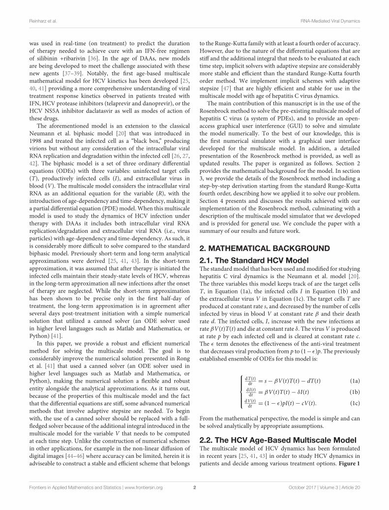
FIGURE 4 | A comparison of the Rosenbrock method with other methods over 14 days of simulation with starting time steps of h = 0.1 and ha = 0.1. The baseline

(the default implementation in the SciPy library of an ODE solver) was computed with time steps of h = 0.001 and ha = 0.01 since with these time step values and

smaller, as expected, all methods converged to the solution of the baseline.

TABLE 7 | Sensitivity of the Rosenbrock method.

Parameter Decreased Increased Parameter Decreased Increased

s 0.88% 1.12% β 0.98% 1.01%

d 1.02% 0.98% δ 1.16% 0.87%

κ 1.08% 0.93% c 1.13% 0.89%

α 0.88% 1.12% ρ 0.93% 1.07%

µ 1.08% 0.93% γ 1.05% 0.96%

Each of the 10 parameters was decreased and increased by 10% of its original value. For

each we present the ratio of the result after 2 days over the result with the original value.

We omit εα and εs since they effectively determine the fraction of α and ρ used in the

model.

to be computed only once. The error term also disregards thevalue of g3.

The scheme for one iteration is shown in Algorithm 1. Animportant observation is how the error term e is computed.It derives only from the error induced by the Rosenbrockiteration, not the computation of the integral term (1 −ǫs)∫∞

0 ρ(a)R(a, t)I(a, t) da.

The system (I/hγ−Jn)gi = f(

yn +∑i−1

j=1 αijgj

)

+1h

∑i−1j=1 γijgj

needs to be solved for four different values of i. Since theleft hand matrix is constant, it is decomposed into its LUdecomposition once. The Jama package [53] is used to performthe LU decomposition for solving the system in a highly efficientmanner.

Algorithm 1: General Rosenbrock Scheme. TOL was set to10−4.

Data: yn, hResult: Compute the next value yn+1 for a step of size hintegralterm← solve (1− ǫs)

∫∞

0 ρ(a)R(a, t)I(a, t) da;LU← LU decomposition of

2 Ih−

(

−d − βVn −βTn

0 −c

)

;

for i← 1 to 4 do

solve for gi: LUgi = f(

yn +∑i−1

j=1 αijgj

)

+1h

∑i−1j=1 γijgj;

end

yn+1 = yn +199 g1 +

12g2 +

25108g3 +

125108g4;

en+1 =1754g1 +

736g2 + 0g3 +

125108g4;

if e ≥ TOL×(yn + f (tn, yn)+ 10−30) thenStart again with smaller h;

else

Increase h;return yn+1

end

4. RESULTS AND DISCUSSION

A preliminary version of the Rosenbrock method was firstimplemented in Python3 using the SciPy library, freely available

Frontiers in Applied Mathematics and Statistics | www.frontiersin.org 7 October 2017 | Volume 3 | Article 20

Reinharz et al. RNA-Mediated Viral Dynamics

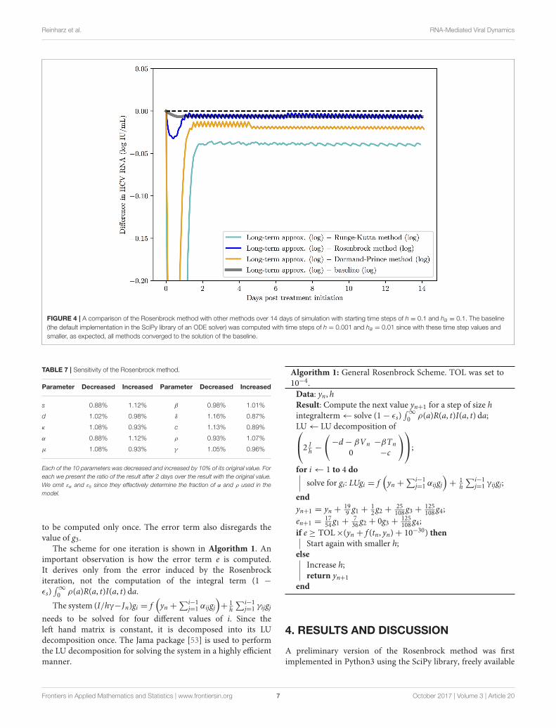
FIGURE 5 | Graphical user interface (GUI). The displayed values are the default options and can be modified. At the bottom are the options to add experimental data

and parameters values from a file. Note that setting the four parameters εα , εs, κ and γ (red fonts) to 0 will keep the system in the pre-treatment steady state. An

option to export the parameters is also available.

at http://www.cs.bgu.ac.il/~dbarash/HCVnumerics, and thenconverted to Java for the purpose of developing a user-friendly simulator with a graphical user interface (GUI)that is freely available at http://www.cs.bgu.ac.il/~dbarash/HCVsimulator. Aside of the Rosenbrock method, the defaultimplementation in SciPy of an ordinary differential solverleverages ODEPACK [54] and is referred to as the canned solverDefault. For this entire section, unless stated otherwise, we usedthe parameters from Rong et al. [41] and shown in Table 4. Theparameters that are changed through the results are the numberof days, the size h of the steps for the ODEs, and the size ha of thesteps for computing the integral. In the case of the Rosenbrockmethod that utilizes an adaptive stepsize, we bound the stepsizeby h as minimum and ha as maximum.

4.1. Short-Term Approximation Holds forHalf a DayThe short-term approximation [41] is shown in Figure 2 in blue.The results are shown for only 2 days since the behavior issmooth and conserved on longer time scales in agreement withprevious results (Figure 2A in [41]). It is clear that after 12 hthe value converges far from the PDE solution. This is expectedsince the effect of the treatment on the infection rate is not

taken into account. In practice, most simulations are valuablefor more than half a day and are focused on the long-termapproximation.

4.2. Long-Term ApproximationUnderestimates PDEIn Rong and Perelson [43] it is hypothesized that the long-term approximation is an underestimate of the PDE modelsolution since some infection events are being ignored. However,with realistic parameters characteristic of potent therapy, thedifference between them is very small. Figure 3 depicts the resultof our scheme, measuring the difference between the long-termapproximation and the solution of the multiscale PDE model(Figure 2B in [41]). We show that the long-term approximationis converging and we are indeed obtaining that the long-termapproximation is an underestimate of the PDE model solution(as the difference between the long term approximation and thesolution of the PDEmodel is negative). The difference of less than0.01 that we are obtaining is very small compared to the y-axisunits shown in Figure 1 of Rong and Perelson [43]. Therefore,it is possible to view in Figure 3 this small effect that is animprovement over what was inferred in Rong and Perelson [43]regarding the long-term approximation. This finding is reiterated

Frontiers in Applied Mathematics and Statistics | www.frontiersin.org 8 October 2017 | Volume 3 | Article 20

Reinharz et al. RNA-Mediated Viral Dynamics

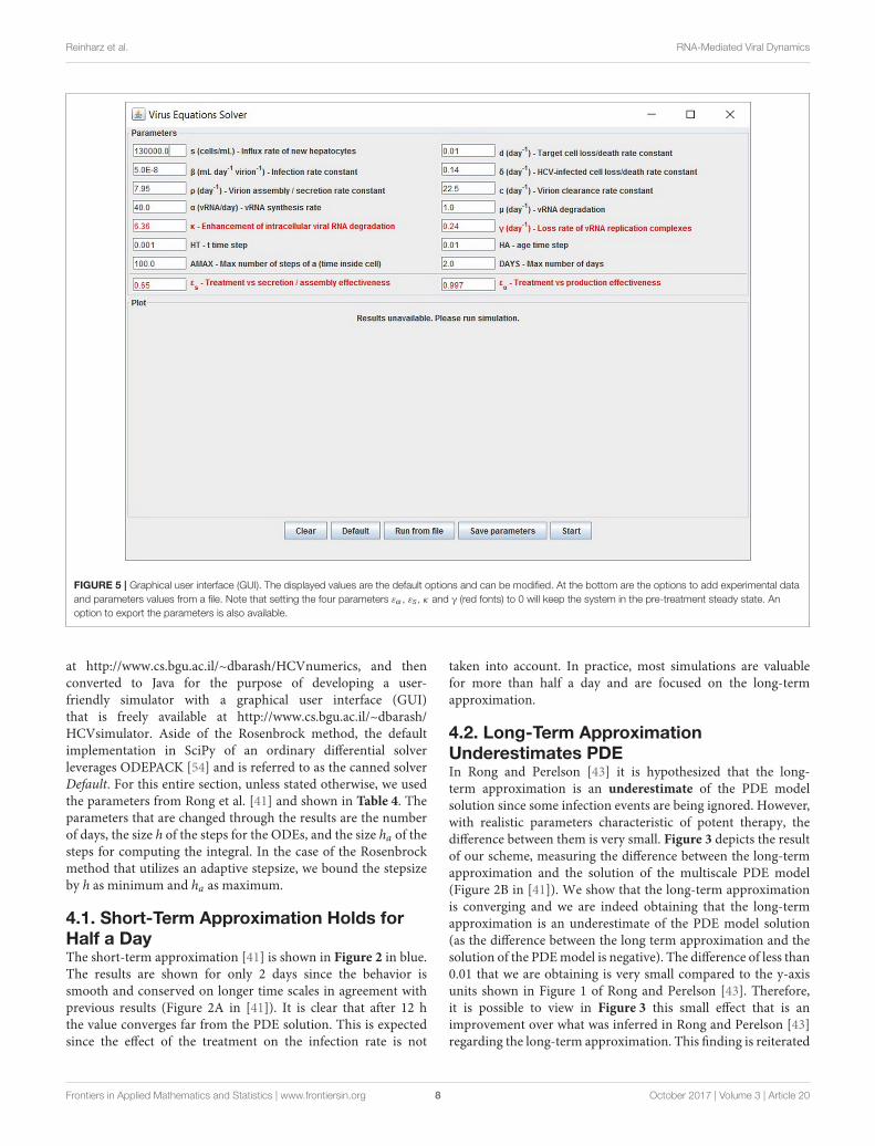
FIGURE 6 | An example of a parameters file that can be automatically

uploaded. Lines starting with a # are comments (ignored). This file can also be

exported from our software, allowing users to share them easily.

here for completeness and is referred to below in the sub-sectionabout the Rosenbrock method.

4.3. The Model Equations Are StiffAn important distinction of the age-based PDE HCV modelequations is their stiffness, or how they can be numericallyunstable even with a small stepsize. We have verified that withsmall time-steps the results are similar for all methods. But aswe increase the size of the steps, the instability of the equationscan be observed over 20 days. All explicit methods such asthe standard version of Runge-Kutta quickly diverge from thesolution with small time-steps. On the other hand an implicitRunge-Kutta method tends to the correct solution and theRosenbrock method does so efficiently as reported below.

4.4. The Rosenbrock Method Is Efficientand StableAs previously mentioned, the integral term (1 −ǫs)∫∞

0 ρ(a)R(a, t)I(a, t) da impedes the use of adaptive stepsizewhen a canned solver is used. Such methods are essential toallow fast computations of complex models like ours. We

present in Table 5 the number of iterations computed usingthe Rosenbrock method, shown in the previous section, incomparison with the default canned method for three differenttime step values of h and ha. With the smallest time step, theRosenbrock method is more than five times as efficient as thedefault canned method, giving results of similar accuracy. Thisis crucial since the methods with fixed time step can take upto tens of seconds per day of simulation with h = 0.001 andha = 0.01. For most research needs, simulations are expectedto be performed numerous times for various instances andparameter values. Under those conditions a five-fold increasein speed, through the decrease in the number of iterations,provides a much needed advantage when testing large number ofparameters over long time periods. Interestingly with the highestvalue of h, the Rosenbrock method takes additional iterations.This is due to the greediness of the time step adjustment, whichwhen increased too quickly and thereby inducing a large errorbacktracks and starts again with a smaller value.

Simpler methods than Rosenbrock exist with adaptivestepsize, such as Dormand–Prince [48], Fehlberg (RKF) [55]and Cash-Karp (RKCK) [56]. These are explicit methods thatcan be easily implemented but are vulnerable to the stiffness ofthe equations, while Rosenbrock is an implicit method that isindeed found to be more stable. In the following comparisonswe demonstrate that the Rosenbrock method is more efficientthan the Runge-Kutta 4th order method and at the same timeit is more stable than both the Runge-Kutta 4th order and theDormand-Prince methods.

First, a comparison of the computing time between theRosenbrock method and the other methods mentioned above isreported in Table 6 with starting time step values of h = 0.001and ha = 0.01 for 14 days of simulation. Each run with acertain method was repeated 10 times, after which the mean andstandard deviation was taken. The Rosenbrock method is over 8times faster than the standard Runge-Kutta 4th order method,which is a non-adaptive time step method. While Dormand–Prince is an adaptive time step method that is even faster thanRosenbrock, as will be shown below, it is an explicit method thatdoes not always converge to the correct solution. The fastest timeof execution for the Dormand-Prince method is not surprisingsince an explicit method is easier to evaluate computationallythan an implicit method, in particular because there is no needfor matrix inversions.

Second, a comparison of the methods behavior over 14 days ofsimulation is presented in Figure 4. All the methods were startedwith time steps of h = 0.1 and ha = 0.1. The baseline (thedefault implementation in the SciPy library of an ODE solver)was computed for h = 0.001 and ha = 0.01 since those timestep values are small enough to ensure that all methods convergeto the same solution. The advantage of the Rosenbrock methodin terms of stability and convergence to the correct solution isclearly noticed.

Finally, we also report in Table 7 the sensitivity of theRosenbrock method. We compute the changed value of theresult after 2 days of simulation given a variation of ±10% on10 parameters. We notice that most of the perturbations aresymmetrical. We omit εα and εs since they effectively determine

Frontiers in Applied Mathematics and Statistics | www.frontiersin.org 9 October 2017 | Volume 3 | Article 20

Reinharz et al. RNA-Mediated Viral Dynamics

FIGURE 7 | Several simulations can be displayed simultaneously. Three treatment scenarios are plotted with similar results as previously shown in Rong et al. [41].

the fraction of α and ρ used in the model. The results (Table 7)indicate that the Rosenbrock method is sufficiently robust for ourneeds.

4.5. The Multiscale Model SimulatorWe have developed a user-friendly simulator with a GUI forthe multiscale model (Figure 5) that is freely available at http://www.cs.bgu.ac.il/~dbarash/HCVsimulator. The parameters fileinput is shown in Figure 6. For illustration, two examplesimulations are provided, one over 2 days (Figure 7) and oneover 28 days (Figure 8). In Figure 7 we show how differentparameter ensembles can be displayed simultaneously. In thatcase we chose εα and εs to be 0 or 0.99, resulting in threecurves. We can observe that increasing the εs parameter, whichdecreases the assembly/secretion of intracellular virions, has astrong short term effect that tempers quickly. In contrast thereduction in the synthesis of vRNA, modeled by an increaseof the parameter εα , shows a slower but more efficient effectthat exhibits stronger results after half a day. Combining bothfactors shows a multiphasic viral decline which was observedunder treatment with HCV NS5A inhibitors [25]. In Figure 8 wepresent the difference between the long-term approximation andthe Rosenbrock method for those three sets of parameters overlonger (than 2 days) treatment durations (e.g., 28 days). Althoughthe highest error is present when εs = 0, the error remains belowa tenth of the differences of the log values. Thus, in all cases the

trends from the first 2 days continue in the next 4 weeks and theerror grows minimally.

5. SUMMARY AND CONCLUSIONS

Modeling intracellular viral RNA dynamics within infectedcells is becoming an improtant mean for considering variouscurative treatment options. A viral dynamic model that considersintracellular viral RNA replication, namely an age-structuredPDE multiscale model, has been recently put forth to studyviral hepatitis dynamics during antiviral therapy [25, 41, 43].This type of model is more complicated to solve than previousODEs models. The seminal works that introduce the age-basedmultiscale model predominantly use analytical approximations,with some numerical solutions that are either based on simplefirst-order methods or canned solvers [25, 41, 43]. Neither ofthese numerical solutions are satisfactory for realistic simulationsof several days of infection and therapy in terms of accuracy,efficiency and stability.

We first showed that the long-term approximation is anunderestimate of the PDE model solution, which was anticipatedin Rong and Perelson [43] because some infection eventsare being ignored in this analytical approximation. We thenobserved that the governing differential equations are stiff andtherefore advanced numerical methods are needed. Methods

Frontiers in Applied Mathematics and Statistics | www.frontiersin.org 10 October 2017 | Volume 3 | Article 20

Reinharz et al. RNA-Mediated Viral Dynamics

FIGURE 8 | Difference in the log values between the long-term approximation [41] and the Rosenbrock method when choosing εα and εs from (0, 0.99). One can

notice how even at the longer treatment duration the difference remains minimal and mostly constant.

with fixed stepsize or alternatively, the use of canned routines,do not offer a comprehensive solution to the model and arelimited in scope. For example, in the multiscale model, thereis an integral term that needs to be computed at each timestep depending on previous iterations and this is inadequatelydone by canned solvers. Methods with adaptive stepsize offera considerable improvement for realistic simulations. Havingpreviously investigated these methods, we found the Rosebrockmethod to be the most accurate and efficient among adaptivestepsize methods for this model. We provide a simulator basedon the Rosenbrock method with a user-friendly GUI that is freelyavailable at http://www.cs.bgu.ac.il/~dbarash/HCVsimulator.

Future work from the numerical standpoint could potentiallyinclude a more comprehensive treatment of the associatedintegral. In particular the adaptive stepsize techniques relyon the evaluation of the error produced at each evaluationof the ODE equations. Therefore, the error produced bythe integral itself is never taken into account. Includingthat term would allow to relax the restrictions on thestepsize increase and potentially decrease further, beyond whatis observed in Table 5 as least number of iterations, thenumber of iterations that are required to achieve a sufficientaccuracy.

The Rosenbrock method implementation provided here canbe generalized to potentially assist in understating treatmentfailure due to drug resistance by the expansion of the age-based model to include viral strains [57]. It could also be usedto explore age-based models that include further aspects ofintracellular HCV life cycle such as translation positive-strandHCV RNA and the synthesis of positive and negative-strandHCV RNA [58]. Finally, since the current age-based HCVmultiscale model is a successful milestone but still fails to predict

cure in some DAA-treated patients [59–61], further modelmodification will be needed [38, 39] and future developmentswould necessitate some updates in the numerical method. Whilesuch models become quickly overwhelming to solve analytically,an extension of the presented method is straightforward. Thesimulator provided here based on the Rosenbrock method can bemodified accordingly and be developed further to accommodatethe modelers needs.

AUTHOR CONTRIBUTIONS

DB conceived research. VR implemented method and developedthe corresponding equations with assistance of DB. VR, HD, andDB designed research. VR, AC, HD, and DB performed researchand wrote the paper.

FUNDING

The research was supported in part by the U.S. National Instituteof Health (NIH) grant R01-AI078881. VR is funded by Azrieliand FQRNT post-doctoral fellowships. The authors would liketo thank the Lynne and William Frankel Center for ComputerSciences at Ben-Gurion University for partially supporting theresearch.

ACKNOWLEDGMENTS

The authors thank Susan Uprichard for careful reading of themanuscript and helpful comments. They would also like to thankLibin Rong and Daniel Coffield for providing the initial code ofthe multiscale model and the reviewers for their comprehensivecomments.

Frontiers in Applied Mathematics and Statistics | www.frontiersin.org 11 October 2017 | Volume 3 | Article 20

Reinharz et al. RNA-Mediated Viral Dynamics

REFERENCES

1. The Polaris Observatory HCV Collaborators. Global prevalence and genotype

distribution of hepatitis C virus infection in 2015: a modelling study. Lancet

Gastroenterol Hepatol. (2017) 2:161–76. doi: 10.1016/S2468-1253(16)30181-9

2. World Health Organization. Guidelines for the Screening, Care and Treatment

of Persons with Hepatitis C Infection. Geneva: World Health Organization

(2014).

3. Martinello M, Gane E, Hellard M, Sasadeusz J, Shaw D, Petoumenos K, et al.

Sofosbuvir and ribavirin for 6 weeks is not effective among people with

recent hepatitis C virus infection: the DARE-C II study. Hepatology (2016)

64:1911–21. doi: 10.1002/hep.28844

4. AASLD/IDSA HCV Guidance Panel. Hepatitis C guidance: AASLD-IDSA

recommendations for testing, managing, and treating adults infected with

hepatitis C virus. Hepatology (2015) 62:932–54. doi: 10.1002/hep.27950

5. Rosen HR. “Hep C, where art thou”: what are the remaining (fundable)

questions in hepatitis C virus research? Hepatology (2017) 65:341–9.

doi: 10.1002/hep.28848

6. Perelson AS. Modelling viral and immune system dynamics. Nat Rev

Immunol. (2002) 2:28–36. doi: 10.1038/nri700

7. Ho DD, Neumann AU, Perelson AS, Chen W, Leonard JM, Markowitz M.

Rapid turnover of plasma virions and CD4 lymphocytes in HIV-1 infection.

Nature (1995) 373:123. doi: 10.1038/373123a0

8. Perelson AS, Neumann AU, Markowitz M, Leonard JM, Ho DD. HIV-1

dynamics in vivo: virion clearance rate, infected cell life-span, and viral

generation time. Science (1996) 271:1582. doi: 10.1126/science.271.5255.1582

9. Burg D, Rong L, Neumann AU, Dahari H. Mathematical modeling of viral

kinetics under immune control during primary HIV-1 infection. J. Theor. Biol.

(2009) 259:751–9. doi: 10.1016/j.jtbi.2009.04.010

10. Ciupe SM, Ribeiro RM, Nelson PW, Dusheiko G, Perelson AS. The role of

cells refractory to productive infection in acute hepatitis B viral dynamics.

Proc Natl Acad Sci USA. (2007) 104:5050–5. doi: 10.1073/pnas.06036

26104

11. Dahari H, Shudo E, Ribeiro RM, Perelson AS. Modeling complex decay

profiles of hepatitis B virus during antiviral therapy.Hepatology (2009) 49:32–

8. doi: 10.1002/hep.22586

12. Nowak MA, Bonhoeffer S, Hill AM, Boehme R, Thomas HC, McDade H.

Viral dynamics in hepatitis B virus infection. Proc Natl Acad Sci USA. (1996)

93:4398–402. doi: 10.1073/pnas.93.9.4398

13. Koh C, Canini L, Dahari H, Zhao X, Uprichard SL, Haynes-Williams

V, et al. Oral prenylation inhibition with lonafarnib in chronic hepatitis

D infection: a proof-of-concept randomised, double-blind, placebo-

controlled phase 2A trial. Lancet Infect Dis. (2015) 15:1167–74.

doi: 10.1016/S1473-3099(15)00074-2

14. Guedj J, Rotman Y, Cotler SJ, KohC, Schmid P, Albrecht J, et al. Understanding

early serum hepatitis D virus and hepatitis B surface antigen kinetics during

pegylated interferon-alpha therapy via mathematical modeling. Hepatology

(2014) 60:1902–10. doi: 10.1002/hep.27357

15. Canini L, Koh C, Cotler SJ, Uprichard SL, Winters MA, Thanda Han MA,

et al. Pharmacokinetics and pharmacodynamics modeling of lonafarnib in

patients with chronic hepatitis delta virus infection. Hepatol Commun. (2017)

1:288–92. doi: 10.1002/hep4.1043

16. Zhang J, Lipton HL, Perelson AS, Dahari H. Modeling the acute and chronic

phases of Theiler murine encephalomyelitis virus infection. J virol. (2013)

87:4052–9. doi: 10.1128/JVI.03395-12

17. Schiffer JT, Abu-Raddad L, Mark KE, Zhu J, Selke S, Magaret A,

et al. Frequent release of low amounts of herpes simplex virus from

neurons: results of a mathematical model. Sci Trans Med. (2009) 1:7ra16.

doi: 10.1126/scitranslmed.3000193

18. Dahari H, Layden-Almer JE, Kallwitz E, Ribeiro RM, Cotler SJ, Layden TJ,

et al. A mathematical model of hepatitis C virus dynamics in patients with

high baseline viral loads or advanced liver disease. Gastroenterology (2009)

136:1402–9. doi: 10.1053/j.gastro.2008.12.060

19. Dahari H, Major M, Zhang X, Mihalik K, Rice CM, Perelson AS, et al.

Mathematical modeling of primary hepatitis C infection: noncytolytic

clearance and early blockage of virion production. Gastroenterology (2005)

128:1056–66. doi: 10.1053/j.gastro.2005.01.049

20. Neumann AU, Lam NP, Dahari H, Gretch DR, Wiley TE, Layden TJ, et al.

Hepatitis C viral dynamics in vivo and the antiviral efficacy of interferon-α

therapy. Science (1998 282:103–7. doi: 10.1126/science.282.5386.103

21. Baccam P, Beauchemin C, Macken CA, Hayden FG, Perelson AS. Kinetics

of influenza A virus infection in humans. J Virol. (2006) 80:7590–9.

doi: 10.1128/JVI.01623-05

22. Pawelek KA, Huynh GT, Quinlivan M, Cullinane A, Rong L, Perelson

AS. Modeling within-host dynamics of influenza virus infection

including immune responses. PLoS Comput Biol. (2012) 8:e1002588.

doi: 10.1371/journal.pcbi.1002588

23. Beauchemin CA, Handel A. A review of mathematical models of influenza A

infections within a host or cell culture: lessons learned and challenges ahead.

BMC Public Health. (2011) 11:S7. doi: 10.1186/1471-2458-11-S1-S7

24. Madelain V, Oestereich L, Graw F, Nguyen THT, De Lamballerie X, Mentré F,

et al. Ebola virus dynamics in mice treated with favipiravir. Antiv. Res. (2015)

123:70–7. doi: 10.1016/j.antiviral.2015.08.015

25. Guedj J, Dahari H, Rong L, Sansone ND, Nettles RE, Cotler SJ, et al. Modeling

shows that the NS5A inhibitor daclatasvir has two modes of action and yields

a shorter estimate of the hepatitis C virus half-life. Proc Natl Acad Sci USA.

(2013) 110:3991–6. doi: 10.1073/pnas.1203110110

26. Dahari H, Sainz B, Perelson AS, Uprichard SL.Modeling subgenomic hepatitis

C virus RNA kinetics during treatment with alpha interferon. J Virol. (2009)

83:6383–90. doi: 10.1128/JVI.02612-08

27. Dahari H, Ribeiro RM, Rice CM, Perelson AS. Mathematical modeling of

subgenomic hepatitis C virus replication in Huh-7 cells. J Virol. (2007)

81:750–60. doi: 10.1128/JVI.01304-06

28. Neumann AU, Phillips S, Levine I, Ijaz S, Dahari H, Eren R, et al. Novel

mechanism of antibodies to hepatitis B virus in blocking viral particle release

from cells. Hepatology (2010) 52:875–85. doi: 10.1002/hep.23778

29. Dahari H, Shudo E, Ribeiro RM, Perelson AS. Mathematical modeling

of HCV infection and treatment. Methods Mol Biol. (2009) 510:439–53.

doi: 10.1007/978-1-59745-394-3_33

30. Dahari H, Guedj J, Perelson AS, Layden TJ. Hepatitis C viral kinetics in the

era of direct acting antiviral agents and interleukin-28B. Curr. Hepatitis Rep.

(2011) 10:214–27. doi: 10.1007/s11901-011-0101-7

31. Snoeck E, Chanu P, Lavielle M, Jacqmin P, Jonsson EN, Jorga K, et al.

A comprehensive hepatitis C viral kinetic model explaining cure. Clin.

Pharmacol. Ther. (2010) 87:706–13. doi: 10.1038/clpt.2010.35

32. Dixit NM, Layden-Almer JE, Layden TJ, Perelson AS.Modelling how ribavirin

improves interferon response rates in hepatitis C virus infection. Nature

(2004) 432:922–4. doi: 10.1038/nature03153

33. Guedj J, Perelson AS. Second-phase hepatitis C virus RNA decline during

telaprevir-based therapy increases with drug effectiveness: implications for

treatment duration. Hepatology (2011) 53:1801–8. doi: 10.1002/hep.24272

34. Dahari H, Canini L, Graw F, Uprichard SL, Araujo ES, Penaranda G, et al.

HCV kinetic and modeling analyses indicate similar time to cure among

sofosbuvir combination regimens with daclatasvir, simeprevir or ledipasvir.

J Hepatol. (2016) 64:1232–9. doi: 10.1016/j.jhep.2016.02.022

35. Gambato M, Canini L, Lens S, Graw F, Londono MC, Uprichard SL, et al.

Modeling early HCV kinetics to individualize direct acting antiviral treatment

duration in patients with advanced cirrhosis. J Hepatol. (2016) 64:S795.

doi: 10.1016/S0168-8278(16)01550-6

36. Dahari H, Shteingart S, Gafanovich I, Cotler SJ, D’Amato M, Pohl RT,

et al. Sustained virological response with intravenous silibinin: individualized

IFN-free therapy via real-time modelling of HCV kinetics. Liver Int. (2015)

35:289–94. doi: 10.1111/liv.12692

37. Rong L, Dahari H, Ribeiro RM, Perelson AS. Rapid emergence of protease

inhibitor resistance in hepatitis C virus. Sci Trans Med. (2010) 2:30ra32.

doi: 10.1126/scitranslmed.3000544

38. Nguyen TH, Guedj J, Canini L, Osinusi A, Pang PS, McHutchison J, et al.

“The paradox of highly effective sofosbuvir combo therapy despite slow viral

decline,” in Conference on Retroviruses and Opportunitstic Infections CROI

2015. Seattle, WA (2015). p. 169–70.

39. Goyal A, Lurie Y, Meissner G, Major M, Sansone N, Uprichard S, et al.

Modeling HCV cure after an ultra-short duration of therapy with direct

acting agents. Antiv Res. (2017) 1444:281–5. doi: 10.1016/j.antiviral.2017.

06.019

Frontiers in Applied Mathematics and Statistics | www.frontiersin.org 12 October 2017 | Volume 3 | Article 20

Reinharz et al. RNA-Mediated Viral Dynamics

40. Guedj J, Dahari H, Uprichard SL, Perelson AS. The hepatitis C virus

NS5A inhibitor daclatasvir has a dual mode of action and leads to a new

virus half-life estimate. Expert Rev Gastroenterol Hepatoly. (2013) 7:397–9.

doi: 10.1586/17474124.2013.811050

41. Rong L, Guedj J, Dahari H, Coffield DJJ, Levi M, Smith P, et al. Analysis

of hepatitis C virus decline during treatment with the protease inhibitor

danoprevir using a multiscale model. PLOS Comput Biol. (2013) 9:e1002959.

doi: 10.1371/journal.pcbi.1002959

42. Guedj J, Neumann AU. Understanding hepatitis C viral dynamics with

direct-acting antiviral agents due to the interplay between intracellular

replication and cellular infection dynamics. J Theor Biol. (2010) 267:330–40.

doi: 10.1016/j.jtbi.2010.08.036

43. Rong L, Perelson AS. Mathematical analysis of multiscale models for hepatitis

C virus dynamics under therapy with direct-acting antiviral agents. Math

Biosci. (2013) 245:22–30. doi: 10.1016/j.mbs.2013.04.012

44. Weickert J, ter Haar Romeny B, Viergever M. Efficient and reliable schemes

for nonlinear diffusion filtering. IEEE Trans Imag Proc. (1998) 7:398–410.

doi: 10.1109/83.661190

45. Barash D, Israeli M, Kimmel R. “An accurate operator splitting scheme

for nonlinear diffusion filtering,” in Proceedings of the 3rd International

Conference on ScaleSpace and Morphology. LNCS Series. Vancouver, BC:

Springer-Verlag (2001). p. 281–9.

46. Barash D. Nonlinear diffusion filtering on extended neighborhood. Appl Num

Math. (2005) 52:1–11. doi: 10.1016/j.apnum.2004.07.002

47. Rosenbrock H. Some general implicit processes for the numerical solution of

differential equations. Comp J. (1963) 5:329–30. doi: 10.1093/comjnl/5.4.329

48. Dormand J, Prince P. A family of embedded Runge-Kutta formulae.

J Comp Appl Math. (1980) 6:19–26. doi: 10.1016/0771-050X(80)9

0013-3

49. Dekker K, Verwer JG. Stability of Runge-Kutta Methods for Stiff Nonlinear

Differential Equations.Vol. 984. North-Holland; Amsterdam: Elsevier Science

Ltd (1984).

50. Kaps P, Rentrop P. Generalized Runge-Kutta methods of order four with

stepsize control for stiff ordinary differential equations. Numer Math. (1979)

33:55–68. doi: 10.1007/BF01396495

51. Hairer E, Wanner G. Solving Ordinary Differential Equations. Vol. 14 of

Springer Series in Computational Mathematics. 2nd ed. Berlin: Cambridge

University Press; Springer-Verlag (1996).

52. PressWH, Teukolsky SH, VetterlingWT, Flannery BP.Numerical Recipes: The

Art of Scientific Computing. 2nd ed. Cambridge, UK: Cambridge University

Press (1997).

53. Hicklin J, Moler C, Webb P, Boisvert RF, Miller B, Pozo R, et al. Jama: A Java

Matrix Package. Available online at: http://mathnistgov/javanumerics/jama

(2000).

54. Hindmarsh AC. ODEPACK, a systematized collection of ODE solvers. IMACS

Trans Sci Comp. (1983) 1:55–64.

55. Fehlberg E. Low-order classical Runge-Kutta formulas with step size control

and their application to some heat transfer problems. NASA Technical Report

315 (1969).

56. Cash J, Karp A. A variable order Runge-Kutta method for initial value

problems with rapidly varying right-hand sides. ACM Trans Math Softw.

(1990) 16:201–22. doi: 10.1145/79505.79507

57. Canini L, Perelson AS. Viral kinetic modeling: state of the art. J Pharmacokinet

Pharmacodyn. (2014) 41:431–43. doi: 10.1007/s10928-014-9363-3

58. Quintela B, Conway J, Hyman J, Reis R, dos Santos R, Lobosco M, et al.

“An age-based multiscale mathematical model of the hepatitis C virus life-

cycle during infection and therapy: including translation and Replication,”

in VII Latin American Congress on Biomedical Engineering CLAIB 2016.

Bucaramanga: Springer (2017). p. 508–11.

59. Lau G, Benhamou Y, Chen G, Li J, Shao Q, Ji D, et al. Efficacy and safety

of 3-week response-guided triple direct-acting antiviral therapy for chronic

hepatitis C infection: a phase 2, open-label, proof-of-concept study. Lancet

Gastroenterol Hepatol. (2016) 1:97–104. doi: 10.1016/S2468-1253(16)30015-2

60. Hasin Y, Shteingart S, Dahari H, Gafanovich I, Floru S, Braun M,

et al. Hepatitis C virus cures after direct acting antiviral-related drug-

induced liver injury: Case report. World J Hepatol. (2016) 8:858–62.

doi: 10.4254/wjh.v8.i20.858

61. Shteyer E, Harel D, Gafanovich I, Dery I, Wolf D, Cottler SJ, et al. End of

treatment RNA-positive/sustained viral response in an individual with acute

hepatitis C virus infection treated with direct-acting antivirals. Therap Adv

Gastroenterol. (2017) 10:429–30. doi: 10.1177/1756283X17694808

Conflict of Interest Statement: The authors declare that the research was

conducted in the absence of any commercial or financial relationships that could

be construed as a potential conflict of interest.

Copyright © 2017 Reinharz, Churkin, Dahari and Barash. This is an open-access

article distributed under the terms of the Creative Commons Attribution License (CC

BY). The use, distribution or reproduction in other forums is permitted, provided the

original author(s) or licensor are credited and that the original publication in this

journal is cited, in accordance with accepted academic practice. No use, distribution

or reproduction is permitted which does not comply with these terms.

Frontiers in Applied Mathematics and Statistics | www.frontiersin.org 13 October 2017 | Volume 3 | Article 20