A REVIEW OF FRICTION FORMULAE IN OPEN CHANNEL FLOW

International Water Technology Journal, IWTJ Vol. 5 –No.1, March 2015

43

A REVIEW OF FRICTION FORMULAE IN OPEN CHANNEL FLOW

Zidan, Abdel Razik Ahmed

Prof. of Hydraulics, Faculty of Engineering, El Mansoura University

E-mail: zidanara @ yahoo.com

ABSTRACT

Due to the lack of analytic representation of frictional resistance in open channels, the

traditional Manning or Chezy equation for steady uniform flow is usually assumed to be suitable as well as a practical representation of frictional resistance expected for unsteady

flow.

No much attention has been given to any other frictional formula in application related to

unsteady non-uniform flow or tidal phenomena in open channels and rivers.

The purpose of this research is to demonstrate the application of alternative equations of resistance, such as the rough turbulent formula, the Williamson equation and the Colebrook

White equation. Differences between, and limitations of each formula are also presented.

An approach to the solution of Colebrook White formula in an explicit form in open

channels is given. A comparative study between this formula and other explicit formulae is

also highlighted.

Received 13 Mar 2015.Accepted1, April 2015

Presented in IWTC 18th

1 REVIEW

1.1 The Chezy formula

In 1768, Antoine Chezy (Rouse, 1957), an engineer of the French Bureau of Bridges and Streets was given the task of designing a canal for the Paris water supply. He reasoned that

the resistance would vary with the wetted perimeter and with the square of velocity, and the

force to balance this resistance would vary with the area of cross section and with the slope.

Therefore, he reasoned that V2 P/(A S ) or V

2/( R S) would be constant for any one channel

and would be the same for any similar channel. His manuscript was not published until 1897,

but his method gradually became known, and the square root of the preceding ratio came to

be known as the Chezy coefficient

The formula can be written as:

RSCV …………………………………………………………………..…… (1)

where:

V : velocity of water;

C : Chezy's coefficient; R : hydraulic radius; and

S : bed slope.

1.2 The Manning Equation

In 1891, another Frenchman, Flamant attributed wrongly to the Irishman R.Manning that C varies with the sixth root of R, although Gauckler in 1868 had proposed the same


44

hypothesis for flat slopes and also Hagen in 1881 attributed the same concept to any slope (

Rouse, 1957).

n

RC

6

1

……….………………………………………………………..…….. (2)

from which

SRn

V 3

21

…………………...………..………………………………………. (3)

where: n is the characteristics of the surface roughness alone and the unit of length used is meter. In 1911 Buckly converted this equation to the foot second unit as

SRn

V 3

2486.1

…………………………………………………………...……. (4)

This equation is known in the English speaking world as the Manning equation, although

on the continent of Europe it is sometimes known as strickler's equation. The Manning

equation has proved most reliable in practical and extremely popular in western countries In order to relate the Manning coefficient (n) and the equivalent particle size (k), Strickler's

empirical formula (1923) was used as ( Henderson, 1966):

k = ( n / 0.034)

6 …………………………………………………………………. (5)

in which (k) in feet

1.3 The Williamson formula

In 1951, James Williamson showed minor but reasonable adjustment to Nikuradse's results (Williamson, 1951) by correcting certain of Nikuradse's calculations and increasing the

assumed grain sizes to allow for thickness of the varnish used to stick the grains, Figure (1),

to the pipe wall. He found that points representating Nikuradse's results fell mush closer than

before to a straight line having slope 1:3. Further he plotted some more observations made by himself, Figure(1), based on his experience with three large concrete line aqueducts and

another of smaller which came under his design and supervision in the Galloway water power

scheme in Scotland.

He found that they fell on a line having the same slope

The Williamson formula is given by:

3

1

18.0

d

kF ……………………………………………………………..………. (6)

3

1

113.0

R

kF …………………………………………………………………….. (7)

where:

F : roughness coefficient;

k : equivalent particle size;

d : diameter of pipe; and R : hydraulic radius


45

Figure 1. Correction of Nikuradse’s data (Williamson, 1951)

1.4 The Colebrook Equation

L. Prandtle and Von Karaman in Germany, and G.I. Tylor in expressing mathematical form the mechanism of turbulence linked the experimental investigation of Nikuradse (1932-

1935) had proved a formula of the type (Colebrook, 1938):

1

113.0log2

1

y

d

F ………………………………………………….…….…… (8)

and showed the lower limit of the integration y1, is a function of the wall particle size k, in the case of rough pipes in which the flow obeys the square resistance law, and is dependent

on the density ρ, the viscosity μ and the shear stress at the wall τ in the case of smooth pipes.

In 1938, Cyril Frank Colebrook confirmed the substitution of values of y, in the foregoing

equation and adopted the following resistance law

(a) Flow in hydraulically smooth pipes:

FRF e

51.2log2

1 …………………..………………………………….……. (9)

(b) Flow in hydraulically rough pipes:

d

k

F 7.3log2

1 ………………………………………………….…………. (10)

And he mentioned that the results of Nikuradse show complete agreement with above two

laws provided certain limiting conditions are satisfied.

F

F

Log r/k

F


46

1.5 Transition Zones

The following formula is used to classify the different types of flow, either smooth,

transition or rough turbulent Rf = V*k/ υ

where:

V* : shear velocity; k : equivalent roughness height; and

υ : kinematics viscosity.

The roughness Reynolds number (Rf) may be expanded into:

VR

R

kFkV

8

* ……………………………………………………………… (11)

in which F is the resistance coefficient, V is the mean velocity and R is the hydraulic radius.

This expansion is a product of three dimensionless numbers, the resistance coefficient, the

relative roughness, and Reynolds number.

The limit of Rf for transition zones has been given by Colebrook (1938) in pipes from 3 to

60, Keulegen and Patterson (1943) has provided this limit in open channels from 3.3 to 67. In

order to remove any uncertainty, others have given the value of Rf for transition zone from 1

to 100. In this present study this value of Rf has been considered from 4 to 100 as given by Henderson (1970). A value of k equal to 0.03 ft (n=0.019) exhibited substantial transition

zones in the river Forth of Scotland for 32 hour tidal wave input. The transition zone occurred

at different places along the river from Stirling to Rosyth.

For k = 0.073 ft (n = 0.022) the transition zone has a negligible influence. A value of

computed Reynolds number for transition zones in the river Forth of Scotland varied between

103 and 10

7 where the maximum Reynolds number was 1.5*10

8 for rough turbulent flow

conditions (Zidan, 1978).

An attempt to express mathematically the transition function for uniform sand roughness is rendered difficulty owing to the fact that the turbulent motion in the Wake behind the grain is

complicated by the mutual interference, and the resistance mechanism made up of viscous

and mechanical force which are difficult to separate. The exact distribution of the function will depend on the distribution of the roughness elements and it is mathematically

indeterminate.

2 COLEBROOK- WHITE EQUATION

2.1 Implicit Colebrook-White Formula

A suggestion by C.M. White for transition formula which similar to those obtained

experimentally for commercial pipes, was simply add together the lower limits of integration y, which satisfy the rough and smooth pipe laws, providing the general formula

For transition regime in which the friction factor varies with both Re and k/d , the equation universally adopted is due to Colebrook and White (1937) as:


47

FRd

k

F e

51.2

7.3log2

1 …………………………………..……..………. (12)

where:

F : roughness coefficient; k : equivalent particle size;

d : diameter of pipe; and

Re : Reynolds number

The Colebrook equation is transcendent and thus can not be solved in terms of elementary

function. Some explicit approximate solutions have been proposed such as:

2.2 Explicit Colebrook-White Formulae

The implicit nature of Colebrook White function (9) has sometimes acted against its adoption in preference to other friction formulae. In 1938 White gave an approximation to the

logarithmic smooth turbulent element in the Colebrook White equation which was compatible

in form with the original one. If Reynolds number is raised to an index could be accepted as a

substitute for Re F in equation (9), then:

8.6log8.1

1 eR

F …………………………………………………..………… (13)

or

61.5log2

19.0

eR

F………..…………………………………………..……….. (14)

Barr Formula (1972) .This type of smooth law approximation has been used by Barr to

form an explicit solution for the Colebrook-White equation

89.0

1286.5

7.3log2

1

eRd

k

F……………………………………………..….. (15)

and for more accuracy (Barr, 1975, 1976):

Relog575.0735.2

Re

7.3log2

1Relog078.0858.0

d

k

F ………………..…………………. (16)

Some Explicit Formulae for Friction Factor in Pipe Flow

Swamee- Jain (1976) ( Genic et al., 2011) : They proposed the equation covering the

range of Re from 5*103 to 10

7 and the relative roughness k/d between 0.00004 and 0.05

as:


48

2

9.0Re

74.5

7.3log

25.0

d

kF …………………………………….………...……… (17)

Round (1980):

5.6Re135.0

Relog8.1

1

d

kF …………………..………………….…….. (18)

Barr (1981) (Beogradau and Brkie, 2012):

7.052.0

29

Re1Re

7

Relog158.5

7.3log2

1

d

kd

k

F ………………….…………..… (19)

Haaland (1983) : Haaland formula is considered as one of the simpler formulae widely

used in the application:

Re

9.6

7.3log8.1

111.1

d

k

F ……………………………..………….….. (20)

Serghides (1984): The equation was based on Steffensen's method. The solution involves

calculation of three intermediate values A, B, and C first, and then substituting those

values into the final solution:

2

2

2

ABC

ABAF ………………………………………………….…….. (21)

where:

983.0Re

12

7.3log2

d

kA

Re

51.2

7.3log2

A

d

kB

Re

51.2

7.3log2

B

d

kC

Manadilli (1997) ( Genic et al., 2011) proposed the following expressions valid for Re

ranging from 5235 to 108 for any value of k/d.

Re

82.96

Re

95

7.3log2

1983.0d

k

F…………………..…………….……….. (22)


49

Gouder and Sommad (2006):

131.0

Re|4587.0ln8686.0

1

s

s

SF………..…………………………….…………. (23)

where Re4587.0lnRe124.0 d

kS

Avci and Karagoz (2009) (Askar et al., 2014):

4.2

101Re001.01lnReln

4.6

dkd

kF ………………………………… (24)

Papaevangelou, Evangleids and Tzimopoulos (2010)

2

9142.0

4

Re

366.7

615.3log

Re)log7(0000947.02479.0

d

kF …………………………………………… (25)

3 COLEBROOK- WHITE EQUATION IN OPEN CHANNELS

3.1 Implicit Solution

For the purpose of analysis of the Colebrook White formula will be written as:

F

b

aR

kc

F Relog

1…………………………………..………………. (26)

One of the first attempts to apply this formula to open channels flow was made in 1938 by

A.P. Zegzhda in Russia (ASCE, 1963). He experimented with rectangular channels roughened

with closely spaced sand grains of ten different sizes, the ratio of sand size to hydraulic radius

varying from 0.125 to 0.2. His plot F versus R was similar to Nikuradse's plot for pipes. Where the Reynolds number was large enough so that F was constant and it was given by

equation (9).

c =- 2.0, a = 11.55 and b = 0.0

Different values for a, b and are also given by different investigators based on experimental results, and finally the task force on friction factors in open channel, ASCE

(1963) has recommended values of c =-2.0, a =12.0 and b = 0.0 for rough turbulent flow and

b = 2.5 for partly rough turbulent flow providing the following two modified equations:


50

R

k

F 12log2

1……………………………………………………………. (27)

FR

k

F Re

5.2

12log2

1………………………………………………….. (28)

Equation (27) is the rough turbulent flow equation for open channel and corresponds to

equation (10) for pipes and equation (29) is the modified Colebrook White equation for open channel which corresponds to equation (12) for flow in pipes.

The modified rough turbulent equation given by ASCE Task Committee (equation) is suitable

for equivalent particle size k > 0.1 ft. i.e. (n > 0.024) (Zidan, 1978)

No much attention has been given to the explicit form of Colebrook White equation for open channels as presented to pipe flow in literature

3.2 Explicit Solution

Zidan's approach (1978)

Plotted data in Figure (2) given by the university of Illionois demonstrate the turbulent

zone corresponds closely to the Blasius Prandtl Von Karman curve. This indicates the law for

turbulent in smooth pipes may be approximately representative of all smooth channels. This

plot also shows that the shape of channel does not have an important influence on friction in turbulent flow

F

Re

Figure2. F-Re Relationship for flow in smooth channels (Chow, 1971)

Bearing in mind that the smooth element in equation (28 ) can be substituted explicitly as

a function of Reynolds number Re as has been done by White, and since the smooth turbulent


51

flow in open channels can be represented by the smooth turbulent flow in pipes as mentioned

before, so the smooth term in equation (28) can be replaced by an empirical term similar to that given by Barr

89.0

1286.5

eR

or

Relog575.0735.2

ReRelog078.0858.0

for more accuracy.

The two approaches for an explicit solution of Colebrook White equation can be written as:

89.0Re

1286.5

12log2

8

1

R

k

g

C

F………………………………………….. (29)

or

Relog575.0735.2

Re

12log2

8

1Relog078.0858.0

R

k

g

C

F…………………..…….….. (30)

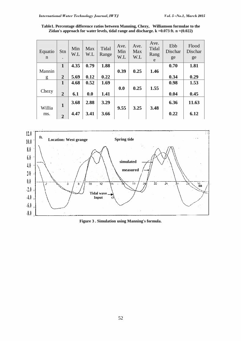
Figures (3) through (6) show simulation of 32 hours tidal wave at Westgrange in the river

Forth using Manning , Chezy, Williamson and the modified Colebrook White (Zidan's

approach) formulae respectively, for the case of rough turbulent flow (n=0.022). It is clear

from these figures that the Manning, the Chezy, and the modified Colebrook White formulae are suitable for rough turbulent flow and there is no appreciable error between these formulae,

Table (1), and have given results near to the actual.

Use of the Williamson formula (7) in the computation produced lower frictional resistance

than the other rough turbulent equations. This being noticeable in producing higher tidal

range and appreciably larger size of hump, Figure (5), this due to smaller relative roughness. 2R/k varies between 200 and 3500 in the Forth. Williamson stated that Nikurades rough

pipe law would not apply d/k value above 500 or 2R/k above 250.

The percentage difference ratio of the Manning, Chezy and Williamson formulae to the modified Colebrook White equation (the Zidan approach) for water levels ,tidal range, and

water discharge at two stations: (1) upstream river Forth ( Westgrange) and the other (2) at

the downstream (Rosyth) is seen in Table (1) for n =0.022 where the transition zones are negligible. As the value of n is reduced to be less than 0.022 or k < 0.073 ft . points of the

tidal cycle fall within the smooth-rough turbulent transition zones. It would seem that the

application of either the Manning, the Chezy, rough turbulent, and the Williamson equations

will produce error in the computations. These errors become substantial for the value of Manning's n less than 0.02 or k < 0.04 ft.


52

Table1. Percentage difference ratios between Manning, Chezy, Williamson formulae to the

Zidan's approach for water levels, tidal range and discharge. k =0.073 ft. n =(0.022)

Figure 3 . Simulation using Manning's formula.

Equatio

n

Stn

.

Min

W.L

Max

W.L

Tidal

Range

Ave.

Min

W.L

Ave.

Max

W.L

Ave.

Tidal

Rang

e

Ebb

Dischar

ge

Flood

Dischar

ge

Mannin

g

1

2

4.35

5.69

0.79

0.12

1.88

0.22

0.39 0.25 1.46

0.70

0.34

1.81

0.29

Chezy

1

2

4.68

6.1

0.52

0.0

1.69

1.41

0.0 0.25 1.55

0.98

0.04

1.53

0.45

Willia

ms.

1

2

3.68

4.47

2.88

3.41

3.29

3.66

9.55 3.25 3.48

6.36

0.22

11.63

6.12

Location: West grange Spring tide

simulated

measured

Tidal wave Input

(Rosyth)

ft.


53

Figure 4 . Simulation using Chezy's formula.

Figure 5 . Simulation using Williamson's formula showing larger humps.

Figure 6 . Simulation using modified Colebrook White's formula (Zidan's approach),

(Zidan, 1978)


simulated

measured

Tidal wave Input (Rosyth)

ft


simulated

measured

Tidal wave Input (Rosyth)

ft.


54

Yen's approach (1991) could be written as:

9.0Re

95.1

12log2

8

1

R

k

g

C

F …………………………………………… (31)

Fenton's approach (2010) could be written as:

9.0

Re

2

12log2

8

1

R

k

g

C

F ………………………………….……… (32)

Both Yen and Fenton formulae are applicable for Re > 3*10

4 and the relative roughness k/R <

0.05.( Fenton, 2010)

Reynolds number term in the numerator 2

0.9 = 1.87 in Fenton equation, for wide channel

not 1.95 as given by Yen. He stated that this value would be smaller for narrow channels.

4 COPARITIVE STUDY

For the sake of comparison between Yen's approach and Zidan's approach, it is assumed that the hydraulic radius (R) varies between 1 m and 20 m and values of Reynolds number Re

varies between 3*104 and 10

8. The modified Colebrook White equation given by Zidan

exhibits smaller values than the corresponding ones using either Yen or Fenton approach.

Table (2) gives a percentage error between both the Yen approach with respect to Zidan's approach which has been tested using actual data of the river Forth of Scotland The results of

this approach has been compared with the corresponding ones of the implicit equation given

by ASCE Task Force on Friction Factor and showed an error of about 0.30 %. Fenton gives a slight higher values than the corresponding ones of Yen formula, for all values of Re as given

by Yen and Fenton (from 3* 104

to 107). This difference may not exceed 1 % in case of

transitional turbulent flow. Increasing the value of hydraulic radius R and Reynolds number

Re will decrease the percentage between the two equations. Increase the value of k will decrease this percentage, Table (4)

Table (3) gives the differences between the three approaches for transition turbulent flow, Reynolds number ranges between 500 and 2000. It is noticed generally that the percentage

error increases than the case of rough turbulent and decreases with the increasing value of Re

.Also it noticed that there a difference between Yen Formula and Zidan approach reaches to about 20.1 % at k = 0.03 ft. and 19.8 % at k = 0.073 ft. for Re = 2000 and hydraulic radius R =

20.

Table 2. Percentage difference ratios of the Yen approach to the Zidan approach for turbulent

flow.

Reynolds

No.

Case

3*104

10 5

106

107

108

k = 0.03 ft.

Maximum error (%) 12.73 9.42 2.66 0.51 0.17

Average error (%) 9.22 5.53 1.14 0.18 0.092

k. = 0.073ft.

Maximum error (%) 9.98 6.97 1.6 0.23 0.12

Average error (%) 4.67 2.63 0.53 0.06 0.04


55

Table 3. Percentage difference ratios of the Yen approach to the Zidan approach for transition

turbulent flow (Re = 500 to 2000).

Reynolds No.

Case

500

1000

1500

2000

k = 0.03 ft.

Maximum error (%) 25.9 20.30 20.21 20.11

Average error (%) 25.33 19.74 19.25 18.88

k = 0.073 ft.

Maximum error (%) 25.72 22.49 21.16 19.81

Average error (%) 24.68 21.07 10.24 17.40

CONCLUSIONS

The Manning and Chezy equations are suitable for simulation of resistance in flow which

are fully rough turbulent. This clear from results obtained in table (1) where the condition of flow is nearly rough turbulent, and the two formulae have given results near to the actual. Use

of the Williamson formula, equation (7) in the computation produced lower frictional

resistance than other rough turbulent equations. This being noticeable in producing higher tidal ranges and appreciably large size of hump in tidal wave due to the smaller relative

roughness. In the river Forth 2R / k varies between 200 and 3500. Williamson stated that the

Nikuradse's rough pipes law would not apply 2R / k value above 250

The Colebrook White equation covers not only the transition region but also the fully

developed smooth and rough open channel as k = 0.0 this reduces the equation for smooth

channel as, k ∞ it forms an equation for rough channels. Unlike the Manning or Chezy equation which should be applied for rough zone only.

The difference between the implicit solution of equation (28) and the explicit solution of equation (29 ) is about 0.3%. The advantage of Colebrook White equation is any big error in

Re, k, or R gives a small error in the value of C due to its logarithmic nature

The Manning formula like the Chezy or the Wlliamson formula is suitable for unsteady varied flow or tidal computation under rough turbulent condition n > 0.023 or k > 0.1 ft.. For

transition turbulent the two equations are no longer suitable, unless these equations are

dependent on Reynolds number Re

The Manning and Chezy equations produce slight difference in the computation at some

places , bearing in mind the two roughness coefficients in the two equations are given by C

=( 1/ n) R1/6

. The difference may indicate that the relationship between n and C may be a function of cross sectional shape or the above relationship is not always proportional to R

1/6

As the value of Manning's n is reduced to less than 0.022 or k < 0.073 ft. points of tidal cycle

fall within the smooth–rough transition zones .It would seem that the application of either the

Manning , Chezy or Williamson equation will produce errors in the computation. These Errors become substantial for the value of Manning ' s n less than 0.02 or k < 0.04 ft.

The Colebrook White explicit equation

89.0

1286.5

12log2

8

1

eRR

k

g

C

F

seems to be suitable for unsteady varied flow and tidal computations in open channels. It

has two advantages, the first being its logarithmic form, i.e for any large error in estimating


56

the value of k will produce only small error in the evaluating of F or C. Secondly it is

suitable for coping with the transition zones especially if these zones are of substantial duration, i.e. more physically correct. It could also be concluded that the partly rough pipes

flow will not behave exactly as partly rough open channel flow.

It will be useful for future work to study the behavior of the friction factor F or C towards

Reynolds's number Re in natural channels like these studies which had been made by

Nikuraadse based on experimental pipes. Since the relation between Reynolds's number Re

and friction factor F or C could be accepted as exponential relationship as mentioned before. It will be useful to trace the transition zones, using formula (11) in natural rivers or open

channels and to draw the relationship between F or C and Re for an average relative

roughness to find the most accurate value for the Index, which could be used for the substitution in the explicit modified Colebrook White equation.

REFERENCES

Askar, M., Turgut, O., and Coban, M. (2014). "A review of non iterative friction

factor correlation for the calculation of pressure drop in pipes", Bitlis, Eren Univ.,

J.Sci & Technol.

Barr, D.I.H. (1972). "New forms of equation for the correlation of pipe resistance

data", Proc.Inst.Civ.Engrs., Part 2, Vol. 53, pp. 333-344.

Barr, D.I.H. (1975). "Two additional methods of direct solution of the Colebrook-

White function", Discussion, Proc.Inst.Civ.Engrs. pp. 827-835.

Barr, D.I.H. (1976). "Two additional methods of direct solution of the Colebrook-

White function", Discussion, Proc.Inst.Civ.Engrs., Part 2, Vol. 61, pp. 489-497.

Barr, D.I.H. (1981). "Solution of the Colebrook–White functions for resistance to

uniform turbulent flow", Proc.Inst.Civ.Engrs., Part 2, Vol. 71.

Brkic, D. (2012). "Determining friction factor in turbulent pipe flow", Chemical

Engineering, pp. 34-39.

Brkic, D. (2012). "Review of explicit approximation to the Colebrook relation for flow friction", J. of Petroleum Science and Engineering, Vol. 77, No.(1), pp.34-48

Chow, V.T. (1971). "Open channel hydraulics", McGraw Hill Book Company Inc.

Colebrook, C.F. (1938-1939). "Turbulent flow in pipes with particular reference to

the transition region between smooth and rough pipe laws", J.Inst.Civ.Engrs., Vol. 10-

12.

Colebrook, C.F. and White, C.M. (1933-1935). "The reduction of carrying capacity

of pipes with age", J.Inst.Civ.Engrs., Vol. 7.

Fenton, J. (2010). "Calculating resistance to flow in open channels", Alternative

Hydraulics, pp. 2 -5.

Genic ,S, Arandjelovic,I, Kalendic, P, Jaric, M, Budimir, Nand Genic, V (2011). "A

review of explicit approximations of Colebrook's equation", FME Transaction,

Belgrade


57

Keulegan,G.H and Pattterson, G.H (1943)." Effect of turbulence and channel

slope on translation waves", Journal of Research of the National Bureau of tandards,Vol.20,June

Haaland, S.E. (1983). "Simple and explicit formulas for the friction factor in turbulent flow", J. of Fluid Engineering, ASME, Vol. 102. No. 5, pp. 657- 664.

Henderson, F.M. (1970). "Open channel flow", McMillan

More, A.A. (2006). "Analytical solutions for the Colebrook and White equation and

for pressure drop in ideal gas flow in pipes", Chemical Engr.Science, Vol. 61, No. 16,

pp. 5515-5519.

Papaevangelo, G., Evanglaids, C. and Tzimopoulos, C. (2010). "Anew explicit

relation for friction coefficient F in the Darcy-Weisbach", Pre: 10, Protection and

Restoration of the Environment, Corfu.

Proudman, J. (1955). "The effect of friction on a progressive wave of tide and surge

in an estuary", Proc.Roy.Soc., London, A, p. 233 and p. 407.

Round, G.F. (1980). "An explicit approximation for the friction factor - Reynolds

number relation for rough and smooth pipes", Can. J. Chem. Eng., Vol.58, pp. 122-123.

Rouse, H.and Ince, S. (1957). "History of hydraulics", Iowa Inst. of Hydraulic

Research.

Serghides, T.K. (1984). "Estimate friction factor accuracy", Chemical Engr., Vol.91,

No. 5, pp.63-64.

Task Force on Friction Factors in Open Channel, J.Hydraulic Div. ASCE, 1963.

Williamson, J. (1951). "The laws of flow in rough pipes", "La Houille Blanche". Vol.6, No. 5, p. 738.

Zidan, A.R. (1978). "A hydraulic investigation of the river Forth", Ph.D. Thesis,

Strathclyde University, Glasgow, U.K.

A REVIEW OF FRICTION FORMULAE IN OPEN CHANNEL FLOW

Documents

Transcript of A REVIEW OF FRICTION FORMULAE IN OPEN CHANNEL FLOW