Computational Statistics and Data Analysis 68 (2013) 52–65

Contents lists available at SciVerse ScienceDirect

Computational Statistics and Data Analysis

journal homepage: www.elsevier.com/locate/csda

A reformulation of the aggregate association index using theodds ratioEric J. Beh ∗, Duy Tran, Irene L. HudsonSchool of Mathematical and Physical Sciences, University of Newcastle, Australia

a r t i c l e i n f o

Article history:Received 29 August 2012Received in revised form 6 June 2013Accepted 6 June 2013Available online 14 June 2013

Keywords:2 × 2 contingency tableAggregate association index (AAI)Chi-squared statisticFisher’s criminal twin dataNew Zealand voting data (1883–1919)

a b s t r a c t

Since its inception in the 1950s the odds ratio has become one of the most simple andpopular measures available for analysing the association between two dichotomous vari-ables. Since the direction andmagnitude of the association can be captured in such a simplemeasure, its impact has been felt throughout much of scientific research, in particular inepidemiology and clinical trials. Despite this, its applicability for analysing aggregate datahas rarely been considered. In this paper we shall express a new measure of association(the aggregate association index, or AAI), in terms of the classic odds ratio. The advantageof doing so is that we are able to explore the use of the odds ratio in a context for whichit was not originally intended, and that is for the analysis of a 2 × 2 table where only theaggregate data is known.

Crown Copyright© 2013 Published by Elsevier B.V. All rights reserved.

1. Introduction

The odds ratio remains one of the most simple, influential and diversely used measures of association available to theanalyst. Due to the widespread use of logistic regression, the odds ratio is widely used in many fields of medical and socialscience research. It is commonly used in survey research, in epidemiology (Rothman, 2002; Rothman et al., 2008) and toexpress the results of some clinical trials, such as in case-control studies (Miettinen, 1976). The odds ratio underpins thefield of meta-analysis (Cheung et al., 2012). Meta analysis is a statistical method used to compare and combine effect sizesfrom a pool of relevant empirical studies. It is now a standard approach to synthesise research findings in many disciplines,including medical and healthcare research, and climate change research (Hudson, 2010) and increasingly in genome-widestudies (Nakaoka and Inoue, 2009; Kraft et al., 2009; Schurink et al., 2012) and drug discovery (Hudson et al., 2012). Theodds ratio is often used as an alternative to the relative risk measure (Zhang and Yu, 1998; Montreuil et al., 2005; Schmidtand Kohlmann, 2008; Viera, 2008) in many applications where it is important to measure the strength, and direction, ofthe association between two dichotomous variables from a 2 × 2 table. Despite its popularity, using the odds ratio in caseswhere only the margins of the 2 × 2 table are available has rarely been considered. One exception to this is Plackett (1977)who showed that the margins do not provide enough information to make inferences about the cell values. There are ahost of techniques that lie within the ecological inference literature that one may consider for inferring cell values, or somefunction of them; none of them, however, consider the odds ratio. For example, King’s (1997) groundbreaking parametricand non-parametric approaches may be considered. King (1997) also describes the ecological inference problem at length.Other strategies include Goodman’s (1953) ecological regression, Freedman et al.’s (1991) neighbourhood model, Chamberand Steel’s (2001) semi-parametric approach, Steel et al.’s (2004) homogeneous model and Wakefield’s (2004) Bayesianextension of this model. A comprehensive review of these ecological inference techniques, and their application to earlyNew Zealand gender and voter turnout data was given by Hudson et al. (2010). Wakefield et al. (2011) further discuss

∗ Corresponding author. Tel.: +61 2 4921 5113.E-mail address: eric.beh@newcastle.edu.au (E.J. Beh).

0167-9473/$ – see front matter Crown Copyright© 2013 Published by Elsevier B.V. All rights reserved.http://dx.doi.org/10.1016/j.csda.2013.06.009

E.J. Beh et al. / Computational Statistics and Data Analysis 68 (2013) 52–65 53

Table 1Notation for a 2 × 2 contingency table.

Column 1 Column 2 Total

Row 1 n11 n12 n1•Row 2 n21 n22 n2•

Total n•1 n•2 n

strategies for determining individual level information based only on aggregate data and Imai et al. (2011) provide an Rpackage, eco, for performing ecological inference.

While these techniques all have their merits, they are all applicable only to the case where multiple, or stratified, 2 × 2tables are simultaneously considered; they cannot used for analysing the aggregate data of a single 2 × 2 table. They alsoinvolve the estimation of simple transformations of the cell frequencies, rather than the general association structure ofthe data. Therefore, all of these techniques are also subject to a variety of untestable assumptions which are problematic forevaluating their effectiveness. It is therefore appropriate to consider a strategy that does not rest on assumptions that are nottestable while being applicable to a single 2× 2 table. Thus, such a strategy should not estimate the (1, 1)’th cell frequency,or some transformation of it, but rather examine the structure of the association between two dichotomous variables basedonly on themarginal information. This issue has a long history and dates back as far as Fisher (1935, p. 48)who focused on thecase where one may ‘‘blot out the contents of the table’’. We shall consider this same issue but examine it by incorporatingthe classic odds ratio into a new index of association called the aggregate association index, also simply referred to as theAAI, proposed by Beh (2008, 2010). It shall be shown that considering the odds ratio offers a simple alternative to consideringthe AAI and whose calculation is as easy as that considered in Beh (2008). This will be achieved in the following 5 sections.Section 2 provides a review of Beh’s (2008, 2010) AAI and Section 3 demonstrates how the odds ratio can be incorporatedinto this measure. The direction of the association structure, when only the marginal information is available is explored inSection 4while Section 5 considers the application of the odds ratio—AAI link using two data sets. The first is the classic twindata of Fisher (1935) and was considered by Beh (2008, 2010) in his development of the AAI. The second 2×2 table is basedon the study conducted by Hudson et al. (2010) and considers data obtained from the 1893 national election held in NewZealand. This data describes the gendered voting rates and is important because it was in this election that New Zealandbecame the first self-governing country in the world where women could vote at the national level. Some final commentsare made in Section 6.

It must be pointed out that it is not the aim of this paper to formulate strategies for making inferences about themagnitude of the odds ratio given only themarginal information. Insteadwe shall use the properties of the odds ratio and theAAI, given only the marginal information of a 2 × 2 contingency table, to explore the association structure of the variables.

2. Aggregate association index

Consider a single two-way contingency table where both variables are dichotomous. Suppose that n individuals/units areclassified into this table such that the number classified into the (i, j)th cell is denoted by nij and the proportion of those inthis cell pij = nij/n for i = 1, 2 and j = 1, 2. Denote the proportion of the sample classified into the i’th row and j’th columnpi• = pi1 + pi2 and p•j = p1j + p2j respectively. Table 1 provides a description of the notation used in this paper.

Typically, measuring the extent to which the row and column variables are associated is achieved by considering thePearson chi-squared statistic calculated from the counts and margins of a contingency table. For a 2 × 2 table of the formdescribed by Table 1, this statistic is

X2= n

(n11n22 − n12n21)2

n1•n2•n•1n•2.

The direction of the association may be determined by considering Pearson’s (1900, p. 12) estimate of his tetrachoric corre-lation. Such an estimate, and one of the most popular measures of correlation for 2×2 contingency tables due to its relativesimplicity is

r =p11p22 − p12p21√p1•p2•p•1p•2

so that X2= nr2.

Another very common measure of association for a 2 × 2 table is the odds ratio (Cornfield, 1951):

θ =n11n22

n21n12. (1)

We shall consider the odds ratio in more detail in Section 3.Suppose, for now, that the cell values of Table 1 are known. Define P1 = n11/n1•; this is the conditional proportion of

an individual/unit being classified into ‘‘Column 1’’ given that they are classified in ‘‘Row 1’’. For the analysis of marginal

54 E.J. Beh et al. / Computational Statistics and Data Analysis 68 (2013) 52–65

Fig. 1. A graphical interpretation of the aggregate association index. The shaded regions reflect the magnitude of the AAI.

information of the 2 × 2 table, most of the ecological inference techniques consider this quantity as did Beh (2008, 2010)for his derivation of the aggregate association index.

When the cell values of Table 1 are unknown, it is not possible to calculate P1. However, the extremes of the permissiblevalues of the (1, 1)th cell frequency are well understood (Duncan and Davis, 1953) to lie within the interval

Ln = max (0, n•1 − n2•) ≤ n11 ≤ min (n•1, n1•) = Un. (2)

Therefore, the bounds for P1 are

LP = max0,

n•1 − n2•

n1•

≤ P1 ≤ min

n•1

n1•, 1

= UP . (3)

Beh (2010) showed that when only marginal information is available, and a test of the association is made at the α level ofsignificance, the bounds of P1 are narrowed to

Lα = max

0, p•1 − p2•

χ2

α

n

p•1p•2

p1•p2•

< P1 < min

1, p•1 + p2•

χ2

α

n

p•1p•2

p1•p2•

= Uα

where χ2α is the 1 − α percentile of the chi-squared distribution with 1 degree of freedom. If Lα < P1 < Uα then there is

evidence that the row and column variables are independent at the a level of significance. However, if LP < P1 < Lα orUα < P1 < UP then there is evidence to suggest that the variables are associated.Within the interval (3), the magnitude of Pearson’s chi-squared varies. Rather than consider whether a statistically signifi-cant association exists (or not) for all possible values of P1 within this interval, the strength of the association may also beconsidered. By doing so, Beh (2008) proposed the following index to assess how likely a statistically significant associationexists between the two dichotomous variables given only the aggregate data:

Aα = 100

1 −

χ2α [(Lα − LP) + (UP − Uα)] +

Uα

LαX2 (P1|p1•, p•1) dP1 UP

LPX2 (P1|p1•, p•1) dP1

(4)

where

X2 (P1|p1•, p•1) = nP1 − p•1

p2•

2 p1•p2•p•1p•2

(5)

is (asymptotically) a chi-squared random variablewith one degree of freedom. The index, Aα , is termed the aggregate associ-ation index (AAI). It quantifies for a givenα how likely a particular set of fixedmarginal frequencieswill enable the analyst toconclude that there exists a statistically significant association between the two dichotomous variables. A value of Aα closeto zero indicates that there is virtually no information in the margins to suggest that an association might exist between thetwo variables. On the other hand, an index value close to 100 reflects that it is highly likely that such an association mayexist. Fig. 1 provides a visual description of the AAI; the magnitude of the AAI is reflected by the shaded area as a proportionof the total area under the curve.

Beh (2010) provided an alternative, and equivalent, expression of (4):

Aα = 100

1 −

χ2α [(Lα − LP) + (UP − Uα)]

kn(UP − p•1)

3− (LP − p•1)

3 −(Uα − p•1)

3− (Lα − p•1)

3

(UP − p•1)3− (LP − p•1)

3

E.J. Beh et al. / Computational Statistics and Data Analysis 68 (2013) 52–65 55

Table 2Fisher’s (1935) criminal twin data.

Convicted Not convicted Total

Monozygotic 10 3 13Dizygotic 2 15 17

Total 12 18 30

Table 3Summary of the 11 NZ elections, 1893–1919.

Year No. of electorates No. of registered men No. of registered women Men’s votes Women’s votes

1893 57 175,915 147,567 126,183 88,4841894 62 191,881 157,942 74,366 47,8621896 62 197,002 142,305 149,471 108,7831899 59 202,044 157,974 159,780 119,5501902 68 229,845 185,944 180,294 138,5651905 76 263,597 212,876 221,611 175,0461908 76 294,073 242,930 238,534 190,1141911 76 321,033 269,009 271,054 221,8781914 76 335,697 280,346 286,799 234,726Apr 1919 76 321,773 304,859 241,524 241,510Dec 1919 76 355,300 328,320 289,244 261,083

where

k =1

3p22•

p1•p2•p•1p•2

.

Due to the popularity of the odds ratio for describing the association between two dichotomous variables, we shall nowexplore the AAI in terms this measure of association. Since the conceptual issues concerned with the interpretation of theAAI remain unchanged, so will Aα when expressed in terms of this ratio—only the parameterisation of the chi-squaredstatistic differs as does the relative level of difficultly of calculating the index. The concept of expressing the strength of theassociation in a 2 × 2 contingency table using the area under curve has been a topic of previous discussion. For example,Glas et al. (2003) discussed the area under the curve (AUC) of a receiver operating characteristic (ROC) function for use inclinical trials—the quantification of this area is based on a plot of true positive rates in a clinical trial against false positiverates. Their discussion of the AUC was made in terms of the odds ratio, as will our discussion of the AAI in the followingsection. However, unlike the AAI, the AUC relies on the cell values of the 2 × 2 table being known.

3. The AAI and the odds ratio

3.1. The odds ratio

One of the most common measures of association for a 2 × 2 contingency table is the odds ratio, (1), which may bealternatively written as

θ =p11p22p21p12

=p11 {p11 − (p1• + p•1 − 1)}

(p1• − p11) (p•1 − p11). (6)

The odds ratio is ameasure of effect size, describing the strength of association, or non-independence, between two dichoto-mous variables. It is commonly used as a descriptive statistic, and plays an important role in logistic regression. Unlike othermeasures of association, such as the relative risk, the odds ratio treats the two variables being compared symmetrically, andcan be estimated using some types of non-random samples. This ratio, originally considered to have been first proposed byCornfield (1951), was considered by Yule (1900, p. 273). However, Yule did not explicitly state it in the above form. Rather,in his discussion of his ‘‘coefficient of association’’ (which is now better known as Yule’s Q ), Yule (1900) considered thereciprocal of the odds ratio which he defined as κ . Other early statistical studies of the odds ratio include, but are not limitedto, Edwards (1957) and Mosteller (1968).

The sample odds ratio, (1), is easy to calculate, and for moderate and large samples, performs well as an estimator of thepopulation odds ratio. Inferences of the population odds ratio may be made by considering Woolf’s (1955) 100(1 − α)%confidence interval

ln (θ) − Zα/2

1n11

+1n12

+1n21

+1n22

, ln (θ) + Zα/2

1n11

+1n12

+1n21

+1n22

(7)

where Zα/2 is (asymptotically) a standard normal random variable.

56 E.J. Beh et al. / Computational Statistics and Data Analysis 68 (2013) 52–65

There is an extensive amount of literature now available on the odds ratio and the coverage of the interval (7). For ex-ample, one may consider Mehta and Walsh (1992), Agresti (1999), Brown (1981) and Lloyd and Moldovan (2007a,b). Morerecently, Demidenko (2012) proposed a simple iterative algorithm that obtains an interval even more narrow than (7), butstill maintaining the same coverage. While Demidenko (2012) focused his attention on the link that the odds ratio has withlogistic regression, his contribution is easily amended for the analysis of a 2 × 2 table. Wilson and Langenberg (1999) alsoconsidered the coverage of the odds ratio from logistic regression. Alternative definitions of the odds ratio (7) including thoseof Woolf (1955), Haldane (1955) and Jewell (1986) may be considered—Walter and Cook (1991) conducted a comparativestudy of these with (1). Anscombe (1981, Chapter 12) and Molenberghs and Lesaffre (1994, p. 636) provided extensions of(1) for a 2×2×2 table. There has been considerable attention given to the calculation of a single odds ratio for stratified 2×2tables. In particular, one may consider those of Woolf (1955) and Mantel and Haenszel (1959) for common approaches andHauck (1989) for an overview of these, and other, measures. Agresti and Coull (2002) discussed, amongst other things, fourdifferent measures of common odds ratio’s for I × J ordered contingency tables and their link to log-linear and associationmodels. Extensive discussions on the odds ratio, including the calculation of its standard error, derivation and coverage ofits confidence issue, have been made by many including Hauck (1989). Excellent overviews of many of these issues may befound by referring to Bishop et al. (1975), Agresti (2002) and Fleiss et al. (2003).

3.2. Patnaik’s expectation

Plackett (1977) demonstrated that, based only on the marginal frequencies of a 2 × 2 contingency table, there is notenough information available to infer themagnitude of the odds ratio. Since the underlying premise of the AAI is not to inferthe magnitude of a measure of association, but rather to determine the strength to which an association might exist, we cantackle our problem by considering the odds ratio, and its natural logarithm, in the following manner.

Consider firstly the expected value, and variance, of n11 suggested by Patnaik (1948, p. 162):

E (n11) =n1•n•1

n+ Var (n11) ln (θ) Var (n11) =

n1•n•1n2•n•2

n2 (n − 1). (8)

Therefore, P1 may be expressed as a function of the log-odds ratio given the marginal information, such that

P1 (ln (θ) |p1•, p•1) = p•1

1 +

n

n − 1

p2•p•2 ln (θ)

. (9)

Note that, for (9), when the row and column variables are independent (i.e. θ = 1), then P1 = p•1. This is also consistentwith commentsmade in the ecological inference, and related, literature; see, for example, Beh (2008) andWakefield (2004).Therefore, by considering (5) and (9) the Pearson chi-squared statistic for a 2 × 2 contingency table can be expressed interms of the log-odds ratio, given the marginal information, by

X2 (ln (θ) |p1•, p•1) = nP1 (ln (θ)) − p•1

p2•

2 p1•p2•p•1p•2

. (10)

Note that substituting (9) into (10) yields the succinct chi-squared function in terms of the log-odds ratio

X2 (ln (θ) |p1•, p•1) =n1•n2•n•1n•2

n (n − 1)2(ln (θ))2 . (11)

From (9), it can be shown that, by taking into consideration the bounds of P1 given by (3), the log-odds ratio is bounded by

Lθ = −

n − 1n

min

1

p1•p•1,

1p2•p•2

< ln (θ) <

n − 1n

min

1

p1•p•2,

1p2•p•1

= Uθ (12)

when only the marginal information is available. Similarly, when only the marginal information is available, and the associ-ation between the two dichotomous variables are being tested at the α level of significance, the log-odds ratio is bounded by

Lα = −

n − 1n

min

1p2•p•2

,

χ2

α

n·

1p1•p2•p•1p•2

< ln (θ)

<

n − 1n

min

p•2

p•1p2•,

χ2

α

n·

1p1•p2•p•1p•2

= Uα. (13)

When Lα < ln (θ) < Uα then there is evidence that the row and column variables are independent at the α level of signifi-cance. However, if Lθ < ln (θ) < Lα or Uα < ln (θ) < Uθ then there is evidence to suggest that the variables are associated.

E.J. Beh et al. / Computational Statistics and Data Analysis 68 (2013) 52–65 57

By incorporating the above log-odds ratio results into the area under the curve defined by (11), but above χ2α , the AAI,

when considering the log-odds ratio, is

Aα = 100

1 −

χ2α

Lα − Lθ

+

Uθ − Uα

+ Uα

LαX2 (ln (θ) |p1•, p•1) d (ln (θ)) Uθ

LθX2 (ln (θ) |p1•, p•1) d (ln (θ))

. (14)

This AAI expression may be simplified by directly evaluating the integrals in this index. By considering (11), when b > a, b

aX2 (ln (θ) |p1•, p•1) d ln (θ) =

13

n1•n•1n•2n2•

n (n − 1)2

b3 − a3

.

Therefore, (14) may be alternatively expressed as

Aα = 100

1 −

χ2α

Lα − Lθ

+

Uθ − Uα

kU3

θ − L3θ −

U3α − L3α

U3θ − L3θ

(15)

where k =13

n1•n1•n2•n•2

n(n−1)2

.

3.3. Solving the quadratic

These results, based onusing the expectation and variance of n11, (8), are appropriate onlywhen the expectation producesa positive result. However, as pointed out by Stevens (1951), Patnaik’s (1948) expectation of n11 can lead to negativequantities. This is clearly inappropriate in some cases and an alternative strategy can be considered.

By rearranging (6) p11 can be expressed as a quadratic function in termsof the odds ratio. Solving this quadratic expressionyields

p11 (θ |p1•, p•1) =θ (p1• + p•1) + (p2• − p•1) −

{θ (p1• + p•1) + (p2• − p•1)}

2− 4p1•p•1θ (θ − 1)

2 (θ − 1)(16)

for θ = 1. This result has been long studied and was considered by, for example, Mosteller (1968, p. 7). More recentlyFleiss et al. (2003, Section 6.6) also considered an expression much like (16) and noted that it provides accurate results forlarge samples. While not working directly with the odds ratio, Yule (1900, p. 273) proposed a similar equation to (16). SinceP1 = p11/p1•, P1 can be expressed in terms of the marginal information and the odds ratio, P1 (θ |p1•, p•1), by

P1 (θ |p1•, p•1) =θ (p1• + p•1) + (p2• − p•1) −

{θ (p1• + p•1) + (p2• − p•1)}

2− 4p1•p•1θ (θ − 1)

2p1• (θ − 1). (17)

Stevens (1951) noted that Patnaik’s expressions are applicable, and valid,when θ → 1 and n → ∞. The impact this propertyhas on the evaluation of the AAI when considering the odds ratio, or log-odds ratio, is negligible when the bounds of θ , orln(θ), are relatively narrow.

4. A positive or negative association?

An advantage of considering the AAI is that, given only the marginal information, Beh (2010) showed that it is possibleto determine whether the association is more likely to be positive or negative. This can be achieved by partitioning Aα suchthat Aα = A+

α + A−α . Here, A

+α is the aggregate positive association index and A−

α is the aggregate negative association index.Given a level of significance a under which a test of association is being made, these quantities measure the extent to whichthe marginal information reflect a significant positive, or negative, association.

When the AAI is expressed in terms of P1, Beh (2010) showed that

A+

α =

UPUα

X2 (P1|p1•, p•1) − χ2

α

dP1 U1

L1X2 (P1|p1•, p•1) dP1

=kn(U1 − p•1)

3− (Uα − p•1)

3− (U1 − Uα) χ2

α

kn(U1 − p•1)

3− (L1 − p•1)

3 ,

A−

α =

UPUα

X2 (P1|p1•, p•1) − χ2

α

dP1 U1

L1X2 (P1|p1•, p•1) dP1

=kn(Lα − p•1)

3− (L1 − p•1)

3− (Lα − L1) χ2

α

kn(U1 − p•1)

3− (L1 − p•1)

3 .

58 E.J. Beh et al. / Computational Statistics and Data Analysis 68 (2013) 52–65

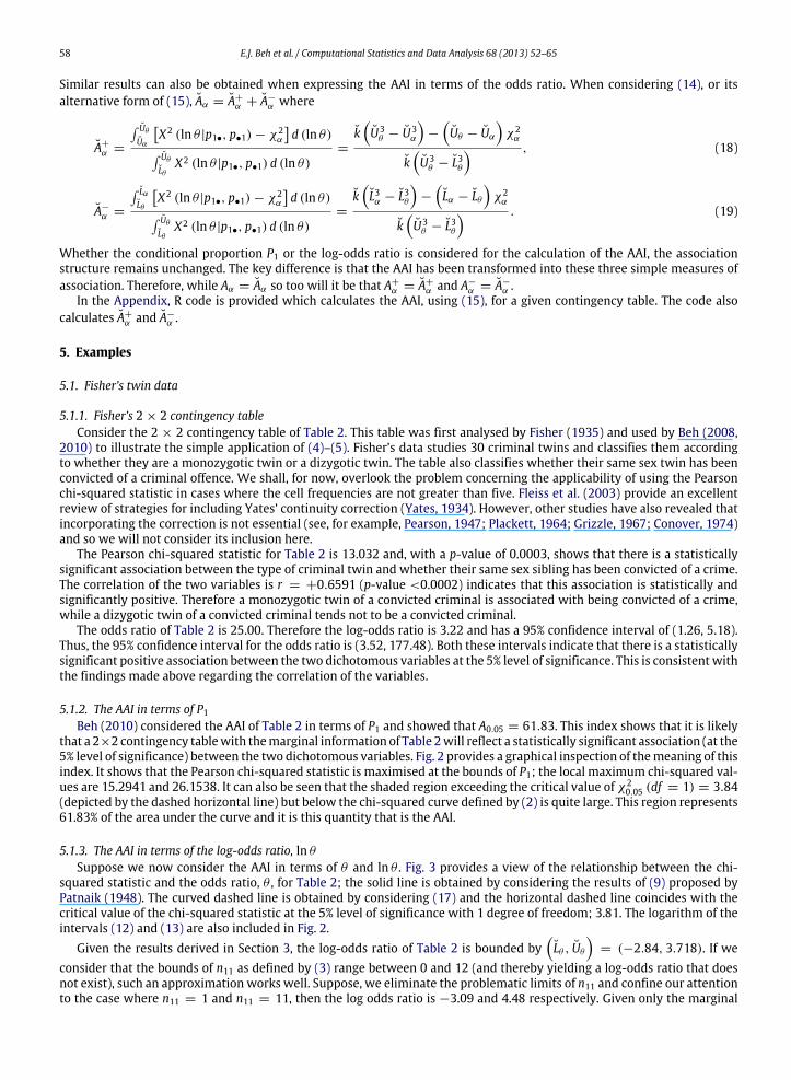
Similar results can also be obtained when expressing the AAI in terms of the odds ratio. When considering (14), or itsalternative form of (15), Aα = A+

α + A−α where

A+

α =

Uθ

Uα

X2 (ln θ |p1•, p•1) − χ2

α

d (ln θ) Uθ

LθX2 (ln θ |p1•, p•1) d (ln θ)

=

kU3

θ − U3α

−

Uθ − Uα

χ2

α

kU3

θ − L3θ , (18)

A−

α =

LαLθ

X2 (ln θ |p1•, p•1) − χ2

α

d (ln θ) Uθ

LθX2 (ln θ |p1•, p•1) d (ln θ)

=

kL3α − L3θ

−

Lα − Lθ

χ2

α

kU3

θ − L3θ . (19)

Whether the conditional proportion P1 or the log-odds ratio is considered for the calculation of the AAI, the associationstructure remains unchanged. The key difference is that the AAI has been transformed into these three simple measures ofassociation. Therefore, while Aα = Aα so too will it be that A+

α = A+α and A−

α = A−α .

In the Appendix, R code is provided which calculates the AAI, using (15), for a given contingency table. The code alsocalculates A+

α and A−α .

5. Examples

5.1. Fisher’s twin data

5.1.1. Fisher’s 2 × 2 contingency tableConsider the 2 × 2 contingency table of Table 2. This table was first analysed by Fisher (1935) and used by Beh (2008,

2010) to illustrate the simple application of (4)–(5). Fisher’s data studies 30 criminal twins and classifies them accordingto whether they are a monozygotic twin or a dizygotic twin. The table also classifies whether their same sex twin has beenconvicted of a criminal offence. We shall, for now, overlook the problem concerning the applicability of using the Pearsonchi-squared statistic in cases where the cell frequencies are not greater than five. Fleiss et al. (2003) provide an excellentreview of strategies for including Yates’ continuity correction (Yates, 1934). However, other studies have also revealed thatincorporating the correction is not essential (see, for example, Pearson, 1947; Plackett, 1964; Grizzle, 1967; Conover, 1974)and so we will not consider its inclusion here.

The Pearson chi-squared statistic for Table 2 is 13.032 and, with a p-value of 0.0003, shows that there is a statisticallysignificant association between the type of criminal twin and whether their same sex sibling has been convicted of a crime.The correlation of the two variables is r = +0.6591 (p-value <0.0002) indicates that this association is statistically andsignificantly positive. Therefore a monozygotic twin of a convicted criminal is associated with being convicted of a crime,while a dizygotic twin of a convicted criminal tends not to be a convicted criminal.

The odds ratio of Table 2 is 25.00. Therefore the log-odds ratio is 3.22 and has a 95% confidence interval of (1.26, 5.18).Thus, the 95% confidence interval for the odds ratio is (3.52, 177.48). Both these intervals indicate that there is a statisticallysignificant positive association between the two dichotomous variables at the 5% level of significance. This is consistentwiththe findings made above regarding the correlation of the variables.

5.1.2. The AAI in terms of P1Beh (2010) considered the AAI of Table 2 in terms of P1 and showed that A0.05 = 61.83. This index shows that it is likely

that a 2×2 contingency tablewith themarginal information of Table 2will reflect a statistically significant association (at the5% level of significance) between the two dichotomous variables. Fig. 2 provides a graphical inspection of themeaning of thisindex. It shows that the Pearson chi-squared statistic is maximised at the bounds of P1; the local maximum chi-squared val-ues are 15.2941 and 26.1538. It can also be seen that the shaded region exceeding the critical value of χ2

0.05 (df = 1) = 3.84(depicted by the dashed horizontal line) but below the chi-squared curve defined by (2) is quite large. This region represents61.83% of the area under the curve and it is this quantity that is the AAI.

5.1.3. The AAI in terms of the log-odds ratio, ln θ

Suppose we now consider the AAI in terms of θ and ln θ . Fig. 3 provides a view of the relationship between the chi-squared statistic and the odds ratio, θ , for Table 2; the solid line is obtained by considering the results of (9) proposed byPatnaik (1948). The curved dashed line is obtained by considering (17) and the horizontal dashed line coincides with thecritical value of the chi-squared statistic at the 5% level of significance with 1 degree of freedom; 3.81. The logarithm of theintervals (12) and (13) are also included in Fig. 2.

Given the results derived in Section 3, the log-odds ratio of Table 2 is bounded byLθ , Uθ

= (−2.84, 3.718). If we

consider that the bounds of n11 as defined by (3) range between 0 and 12 (and thereby yielding a log-odds ratio that doesnot exist), such an approximation works well. Suppose, we eliminate the problematic limits of n11 and confine our attentionto the case where n11 = 1 and n11 = 11, then the log odds ratio is −3.09 and 4.48 respectively. Given only the marginal

E.J. Beh et al. / Computational Statistics and Data Analysis 68 (2013) 52–65 59

Fig. 2. Plot of X2 (P1|p1• = 12/30, p•1 = 13/30) versus P1 for Table 2.

Fig. 3. Plot of X2 (θ |p1• = 12/30, p•1 = 13/30) versus θ for Table 2. The solid line based on (9), and the dashed (curved) line based on (17).

information, and (13), if we were to test the association structure of the two dichotomous variables at the 5% level of signifi-cance, statistical independence occurs when the log-odds ratio is bounded by the interval

L0.05, U0.05

= (−1.425, 1.425).

A graphical comparison of the relationship between the chi-squared statistic and the log-odds ratio is given by Fig. 4; thedashed horizontal line in this figure is, again, the critical value of the chi-squared statistic at the 5% level of significance—χ20.05 (df = 1) = 3.84.One can see that when considering the relationship between the chi-squared statistic and the log-odds ratio as defined

by (9) and (17), they are very similar when comparedwith its alternative result, especially when the odds ratio is confined tolie within the interval

L0.05, U0.05

. Any deviation between (9) and (17) exists at the bounds of the log-odds ratio

Lθ , Uθ

.

Thus, the AAI may be accurately, and simply, derived using (14), or alternatively (15). Now,

k =13

13 × 17 × 12 × 18

30 × 292

= 0.6307.

Therefore, when testing the association between the two variables of Table 2 at the 5% level of significance, the AAI is,from (15),

A0.05 = 100

1 −

3.84 × [(−1.425 + 2.84) + (3.718 − 1.425)]

0.6307 ×3.7183

− (−2.84)3 −

1.4253− (−1.425)3

3.7183− (−2.84)3

= 61.83.

This is exactly the same as the AAI derived when considering P1. R code is provided in the Appendix to calculate the AAI,when considered as a function of the log-odds ratio. This code also calculates the positive and negative contributions of theAAI as defined by equations (18) and (19) which we shall consider in Section 5.1.4.

60 E.J. Beh et al. / Computational Statistics and Data Analysis 68 (2013) 52–65

Fig. 4. Plot of X2 (ln θ |p1• = 12/30, p•1 = 13/30) versus ln θ for Table 2. The solid line based on (9), and the dashed (curved) line based on (17).

Table 4Cross-classification of registered voters by gender for 1893.

Vote No vote Total

Women 88,484 59,083 147,567Men 126,183 49,732 175,915

Total 214,667 108,815 323,482

Fig. 4, and A0.05 = 61.83, shows that, given the marginal information only of Table 2, there appears to be some evidencethat a strong association exists. This is evident by considering the area under the solid curve that lies above the critical valueof 3.84 but for the log-odds ratio confined to its bounds. Despite the continuous nature of the odds ratio in our discussion, it isproblematic to quantifying the AAI using (17). However, by considering plots of the form that Fig. 4 takes, we can determinethat the AAI is bounded such that

AAIα < 1001 −

12

χ2

α (df = 1)X2 (P1 (ln θ) = Lα)

+χ2

α (df = 1)X2 (P1 (ln θ) = Uα)

.

For Table 2, this suggests that if one considers its log-odds ratio given only the marginal information, the upper bound forthe AAI at the 0.05 level of significance is

AAI0.05 < 1001 −

12

3.84

15.2941+

3.8426.1538

= 80.1.

In fact, by considering a log-odds ratio greater than zero, we can see that the area under the curve is far greater than the areaunder the curve when the log-odds ratio is negative. This suggests that, not only is there strong evidence of a statisticallysignificant association between the two dichotomous variables at the α level of significance, but that the association is morelikely to be positive than negative.

5.1.4. The direction of the associationIrrespective of which simplemeasure of association is considered, the AAI is 61.83 and concludes that, given themarginal

information, it is likely that there is a statistically significant association at the 5% level of significance. The question now iswhether we can determine the direction of the association.

Suppose we first consider the AAI in terms of P1. By partitioning the AAI such that Aα = A+α +A−

α we see that A+α = 46.43

and A−α = 15.40. Beh (2010) determined these quantities which suggests that the association is three times more likely

to be positive than negative. We may also determine these quantities when considering the log-odds ratio by deriving thepartition Aα = A+

α + A−α . As we described above, since these AAI terms are related by a simple reparameterisation, we find

that A+α = A+

α = 46.43while A−α = A−

α = 15.40. Themagnitude of these aggregate positive and negative association indices

E.J. Beh et al. / Computational Statistics and Data Analysis 68 (2013) 52–65 61

Fig. 5. Plot of X2 (θ |p1•, p•1) versus θ for Table 4 using (9).

is reflected by the relatively large area above the critical value, but below the AAI curves, of Fig. 4 taking into considerationthe bounds associated with ln θ .

5.2. New Zealand voting data, 1893–1919

The history of the New Zealand (NZ) election system is an interesting one because, in 1893, it is the first self-governingnation in the world to grant women the right to vote in federal elections; even though they were not eligible to standas candidates until 1919. The trend was quickly spread across the globe including Australia: South Australia enfranchisedwomen in 1894, Western Australia in 1899, and the Australian Commonwealth government in 1902. One may consult thefollowing URL www.elections.org.nz/study/education-centre/history/votes-for-women.html for an extensive history of thevoting status for women in NZ. Further information may be found by consulting Moore (2005).

The data from the NZ federal elections held between 1893 and 1919 provides a wealth of information for the analysisof early voting behaviour. For each year that a national election was held, Table 3 provides a summary of the number ofmen and women voters as well as the number of registered voters for each gender. This table is derived from Table 1 ofHudson et al. (2010). Fortunately for analysts studying this issue, data at the electorate level were also kept that records thegender of those that voted and those that did not. An example of this data can be seen by considering Table 4which providesa summary of the men and women who registered to vote in the 1893 election. A more comprehensive discussion of theapplication of the AAI (in terms of P1) to the New Zealand voting data of Table 3 was made by Tran et al. (2012).

If we consider for the moment that the cell values of Table 2 are known, the Pearson chi-squared statistic is 4978.115and, with a p-value <0.0001, shows that there is a statistically significant association between gender and whether thevoter turned out to vote in the 1893 election. It must be noted that the very large sample size has influenced the very largechi-squared statistic, thus we would expect that, for an analysis of the marginal information only, the AAI to be very high.However, it is the direction of the association that is of interested to us here for this data. We can see that 88484/147567,or 60% of women voted compared with 71.7% of men.

Based on the counts in Table 4, women are 88484/59083 = 1.49 times more likely to vote than not vote. Similarly, menare 126183/49732 = 2.53 times more likely to vote than not vote. Therefore, with an odds ratio of 1.49/2.53 = 0.59 thusa women are 0.59 times more likely to vote than a male (we may more succinctly express this by saying that, for the 1893New Zealand election, males were 1.7 times more likely to vote than females). Therefore the log-odds ratio is −0.527 andhas a 95% confidence interval of (−0.54, −0.51). Thus, the 95% confidence interval for the odds ratio is (0.58, 0.60). Boththese intervals indicate that there is a statistically significant negative association between the two dichotomous variablesof Table 4 at the 5% level of significance. The 95% confidence interval of the log-odds ratio also suggests that the associationbetween gender and voting status is negative. Therefore, analysing Table 4with the cell values assumed known, this intervalsuggests that there are statistically significantly more men voting that females.

Consider now the case where only the marginal information of Table 4 is known. Not surprising the AAI is 99.9932suggesting that there is ample evidence in the marginal frequencies of Table 4 to suggest that the association between thetwo dichotomous variables is statistically significant at the 0.05 level of significance. Again, this is largely due to the largesample size for the 1893 election. Fig. 5 provides a plot of the odds ratio against the Pearson chi-squared statistic for Table 4;the dashed horizontal line is where χ2

0.05 (df = 1) = 3.84. Fig. 6 gives an analogous plot but considers the log-odds ratio.We can, however, confine our attention to whether the association is likely to be a positive or negative by considering

Eqs. (18) and (19). Fig. 6 suggests that when considering the relationship between gender and voting status of Table 4, andkeeping in mind the reformulation of the AAI in terms of the odds ratio, the association is far more likely to be negative thanpositive. Using the R code given in the Appendix we indeed find that A+

α = 37.11 and A−α = 62.88. Such figures suggest that,

based only on themarginal information of Table 4, the association between gender and voter turnout is far more likely to benegative than positive. Therefore, based only on the marginal information, these quantities suggest that the proportion of

62 E.J. Beh et al. / Computational Statistics and Data Analysis 68 (2013) 52–65

Fig. 6. Plot of X2 (θ |p1•, p•1) versus ln θ for Table 4 using (9).

voters is more likely to be male than female; this is consistent with our findings when the cell values of Table 4 are assumedknown. From an ecological inference perspective, the estimated values of the gendered proportions studied by Hudson et al.(2010) agree that males were more likely than females to vote in the 1893 national election held in New Zealand.

6. Discussion

This paper has discussed the reformulation of the aggregate association index in terms of the odds ratio and log-oddsratio for a single 2×2 contingency table. By considering the index in this manner, we can identify how likely two categoricalvariables will be associated based only on the marginal frequencies. However, measures of association, other than the oddsratiomay also be considered by incorporating Edwards’ criteria (Edwards, 1957). This criterion suggests that, for the analysisof 2×2 tables, measures of association should be expressible as functions of the odds ratio.While Edwards (1957) originallyconsidered his study when the marginal totals are not assumed fixed, the criterion may be considered in the context of theAAI. Bishop et al. (1975, p. 378) suggest that such a relationship be structured so that

g (θ) =f (θ) − 1f (θ) + 1

where f (θ) is an invertible and monotonically increasing function in terms of the odds ratio, θ , and g (θ) is a measure ofassociation. For example, when f (θ) = θ , f (θ) =

√θ , f (θ) = θπ/4, f (θ) = θ3/4, g (θ) is Yule’s Q (or ‘‘coefficient of

association’’; Yule, 1900, p. 272), Yule’s Y (or ‘‘coefficient of colligation’’; Yule, 1912, p. 592), Edwards’ J (Edwards, 1957) andDigby’sH (Digby, 1983, p. 754) respectively. All thesemeasures of association are designed to estimate (with varying degreesof accuracy) Pearson’s (1900) tetrachoric correlation. One may also consider global measures of association other thanPearson’s chi-squared statistic, such as the Goodman–Kruskal tau index for asymmetrically structured variables (Goodmanand Kruskal, 1954). Such generalisations require a more lengthy discussion of the issues that have been made here and sowill be left for future consideration.

Preliminary work has been undertaken to investigate the extension of the AAI for multiple 2×2 tables (Tran et al., 2012)when considered in terms of P1. Thus, extending the current discussion to multiple 2 × 2 tables by incorporating commonodds ratios such as the Mantel–Haenszel and Woolf estimate is an avenue for future consideration. Establishing the linksbetween the AAI and the Cochran–Mantel–Haenszel (CMH) test can also be considered.

One must note that the AAI we have considered here implies that the odds ratio and the log-odds ratio are continuous.Strictly speaking, since there are a discrete number of values that n11 may take, there are also a discrete number of valuesthat θ can be. Therefore adjusting the AAI to take into consideration this characteristic can bemade. Although, as Beh (2010)shows, there is little difference if one considers a continuous or discrete version of the AAI, especially when the intervallength of (1) is wide and/or the sample size is large. Further consideration of this issue will also be left for future discussion.

E.J. Beh et al. / Computational Statistics and Data Analysis 68 (2013) 52–65 63

Acknowledgement

Wewould like to thank Dr. Linda Moore (Statistics New Zealand) for making available the 1893 New Zealand voting datathat is the focus of the application in Section 5.2.

Appendix. R code

Here we shall give R code that calculates the AAI when expressed in terms of the log-odds ratio. It does so using Eq. (15)and incorporates the bounds of (12) and (13). The analyst only needs to specify the contingency table, N , being analysed andthe level of significance alpha; by default alpha is set at 0.05. The code includes as its output the AAI (defined by Eq. (15),A+

α and A−α ).

AAIlogtheta <- function(N, alpha = 0.05){

n <- sum(N)p<- N/n

prows <- apply(p, 1, sum)pcols <- apply(p, 2, sum)

# Critical value of the chi-squared statistic with one degree# of freedom and the alpha level of significance

critchisq <- qchisq(1 - alpha, 1)

# The bounds of ln(theta); given by equation (12)#

Ltheta <- -((n - 1)/n) * min(1/(prows[1] * pcols[1]),1/(prows[2] * pcols[2]))

Utheta <- ((n - 1)/n)*min(1/(prows[1] * pcols[2]), 1/(prows[2]* pcols[1]))

# The bounds of ln(theta), when testing the association at the# alpha level of significance; given by equation (13)

Lalpha <- -((n - 1)/n)*min(1/(prows[2] * pcols[2]),sqrt(critchisq/(n * prows[1] * prows[2] * pcols[1] *pcols[2])))

Ualpha <- ((n - 1)/n) * min(pcols[2]/(prows[1] * prows[2]),sqrt(critchisq/(n * prows[1] * prows[2] * pcols[1] *pcols[2])))

k <- (1/3) * ((n^3 * prows[1] * prows[2] * pcols[1] *pcols[2])/((n - 1)^2))

# The positive and negative quantities of the AAI; given by# equations (18) and (19) respectively

AAIpos <- 100 * (k * (Utheta^3 - Ualpha^3) - (Utheta - Ualpha)* critchisq)/( k *(Utheta^3 - Ltheta^3))

AAIneg <- 100 * (k * (Lalpha^3 - Ltheta^3) - (Lalpha - Ltheta)* critchisq)/(k * (Utheta^3 - Ltheta^3))

# The AAI, our quantity of interesting lying between 0 and 100

AAI <- AAIpos + AAIneg

64 E.J. Beh et al. / Computational Statistics and Data Analysis 68 (2013) 52–65

return(list(AAIpos = AAIpos, AAIneg = AAIneg, AAI = AAI))

}

For example, supposewe consider Fisher’s (1935) twin data of Table 2. Then, expressing it as the R object fisher.dat suchthat

> fisher.dat<- matrix(c(10,2,3,15), nrow = 2)> dimnames(fisher.dat) <- list(paste(c("Monozygotic","Dizygotic")),+ paste(c("Convicted","Not Convicted")))> fisher.dat

Convicted Not ConvictedMonozygotic 10 3Dizygotic 2 15

>

Therefore, we may calculate the AAI and its positive and negative terms by

> AAIlogtheta(fisher.dat)$AAIposMonozygotic

46.43128

$AAInegMonozygotic

15.39580

$AAIMonozygotic

61.82707

>

References

Agresti, A., 1999. On logit confidence intervals for the odds ratio with small sample. Biometrics 55, 597–602.Agresti, A., 2002. Categorical Data Analysis, second ed. Wiley, NJ.Agresti, A., Coull, B.A., 2002. The analysis of contingency tables under inequality constraints. Journal of Statistical Planning and Inference 107, 45–73.Anscombe, F., 1981. Computing in Statistical Science through APL. SpringerVerlag, New York.Beh, E.J., 2008. Correspondence analysis of aggregate data: the 2 × 2 table. Journal of Statistical Planning and Inference 138, 2941–2952.Beh, E.J., 2010. The aggregate association index. Computational Statistics & Data Analysis 54, 1570–1580.Bishop, Y.M., Fienberg, S.E., Holland, P.W., 1975. Discrete Multivariate Analysis: Theory and Practice. MIT Press, Cambridge, MA.Brown, C.C., 1981. The validity of approximation methods for interval estimation of the odds ratio. American Journal of Epidemiology 113, 474–480.Chambers, R.L., Steel, D.G., 2001. Simple methods for ecological inference in 2 × 2 tables. Journal of the Royal Statistical Society, Series A 164, 175–192.Cheung, M.W.-L., Ho, R.C.M., Lim, Y., Mak, A., 2012. Conducting a meta-analysis: basics and good practices. International Journal of Rheumatic Diseases 15,

129–135.Conover,W.J., 1974. Some reasons for not using Yates continuity correction on 2×2 contingency tables (with discussion). Journal of the American Statistical

Association 69, 374–382.Cornfield, J., 1951. Amethod of estimating comparative rates from clinical data: applications to cancer of the lung, breast, and cervix. Journal of the National

Cancer Institute 11, 1269–1275.Demidenko, E., 2012. The shortest width confidence interval for odds ratio in logistic regression. Open Journal of Statistics 2, 305–308.Digby, P.G.N., 1983. Approximating the tetrachoric correlation coefficient. Biometrics 39, 753–757.Duncan, O.D., Davis, B., 1953. An alternative to ecological correlation. American Sociological Review 18, 665–666.Edwards, A.W.F., 1957. A note on the practical interpretation of 2 × 2 tables. British Journal of Preventative and Social Medicine 11, 73–78.Fisher, R.A., 1935. The logic of inductive inference (with discussions). Journal of the Royal Statistical Society, Series A 98, 39–82.Fleiss, J.L., Levin, B., Paik, M.C., 2003. Statistical Methods for Rates and Proportions, third ed. Wiley, NJ.Freedman, D.A., Klein, S.P., Sacks, J., Smyth, C.A., Everett, C.G., 1991. Ecological regression and voting rights. Evaluation Review 15, 673–711.Glas, A.S., Lijmer, J.G., Prins, M.H., Bonsel, G.J., Bossuyt, P.M.M., 2003. The diagnostic odds ratio: a single indicator of test performance. Journal of Clinical

Epidemiology 56, 1129–1135.Goodman, L.A., 1953. Ecological regressions and behavior of individuals. American Sociological Review 18, 663–664.Goodman, L.A., Kruskal, W.H., 1954. Measures of association for cross classifications. Journal of the American Statistical Association 49, 732–764.Grizzle, J.E., 1967. Continuity correction in the χ2 for 2 × 2 tables. The American Statistician 21 (October), 28–32.Haldane, J.B., 1955. The estimation and significance of the logarithm of a ratio of frequencies. Annals of Humam Genetics 20, 309–311.Hauck, W.W., 1989. Odds ratio inference from stratified samples. Communications in Statistics—Theory and Methods 18, 767–800.Hudson, I.L., 2010. Meta-analysis and its application in phonological research: a review and new statistical approaches. In: Hudson, I.L., Keatley, M.R. (Eds.),

Phenological Research: Methods for Environmental and Climate Change Analysis. Springer, Dordrecht, pp. 463–509.Hudson, I.L., Moore, L., Beh, E.J., Steel, D.G., 2010. Ecological inference techniques: an empirical evaluation using data describing gender and voter turnout

at New Zealand elections, 1893–1919. Journal of the Royal Statistical Society, Series A 173, 185–213.

E.J. Beh et al. / Computational Statistics and Data Analysis 68 (2013) 52–65 65

Hudson, I.L., Shafi, S., Lee, S., Hudson, S., Abell, A., 2012. Druggability in drug discovery: self organising maps with a mixture discrimination approach. In:Australian Statistics Conference, Adelaide.

Imai, K., Lu, Y., Strauss, A., 2011. Eco: R package for ecological inference in 2 × 2 tables. Journal of Statistical Software 42, 23.Jewell, N.P., 1986. On the bias of commonly used measures of association for 2 × 2 tables. Biometrics 42, 351–358.King, G., 1997. A Solution to the Ecological Inference Problem. Princeton University Press, Princeton.Kraft, P., Wacholder, S., Cornelis, M.C., Hu, F.B., Thomas, G., Hoover, R., Hunter, D.J., Chanock, S., 2009. Beyond odds-ratios—communicating disease risk

based on genetic profiles. Nature Reviews Genetics 10, 264–269.Lloyd, C.J., Moldovan, M.V., 2007a. Unconditional efficient one-sided confidence limits for the odds ratio based on unconditional likelihood. Statistics in

Medicine 26, 5136–5146.Lloyd, C.J., Moldovan,M.V., 2007b. Exact one-sided confidence bounds for the risk ratio in 2×2 tableswith structural zero. Biometrical Journal 49, 952–963.Mantel, N., Haenszel, W., 1959. Statistical aspects of the analysis of data from retrospective studies of disease. Journal of the National Cancer Institute 22,

719–748.Mehta, C.R., Walsh, S.J., 1992. Comparison of exact, mid-p, and Mantel–Haenszel confidence intervals for the common odds ratio across several 2 × 2

contingency tables. The American Statistician 46, 146–150.Miettinen, O.S., 1976. Estimability and estimation in case-referent studies. American Journal of Epidemiology 103, 226–236.Molenberghs, G., Lesaffre, E., 1994.Marginalmodeling of correlated ordinal data usingmultivariate Plackett distribution. Journal of the American Statistical

Association 89, 633–644.Montreuil, B., Bendavid, Y., Brophy, J., 2005. What is so odd about odds? Canadian Journal of Surgery 48, 400–408.Moore, L., 2005. Was gender a factor in voter participation at New Zealand elections? In: Fairburn, M., Olssen, E. (Eds.), Class, Gender and the Vote. Otago

University Press, Otago, NZ, pp. 129–142.Mosteller, F., 1968. Association and estimation in contingency tables. Journal of the American Statistical Association 63, 1–28.Nakaoka, H., Inoue, I., 2009. Meta-analysis of genetic association studies: methodologies, between-study heterogeneity and winner’s curse. Journal of

Human Genetics 54, 615–623.Patnaik, P.B., 1948. The power function of the test for the difference between two proportions in a 2 × 2 table. Biometrika 35, 157–173.Pearson, E.S., 1947. The choice of statistical tests illustrated on the interpretation of data classed in a 2 × 2 table. Biometrika 34, 139–167.Pearson, K., 1900. Mathematical contributions to the theory of evolution VII: on the correlation of characters not quantitativelymeasureable. Philosophical

Transactions of the Royal Society of London, Series A 195, 1–47.Plackett, R.L., 1977. The marginal totals of a 2 × 2 table. Biometrika 64, 37–42.Plackett, R.L., 1964. The continuity correction in 2 × 2 tables. Biometrika 51, 327–337.Rothman, K., 2002. Epidemiology: An Introduction. Oxford University Press, Oxford, England.Rothman, K.J., Greenland, S., Lash, T.L., 2008. Modern Epidemiology, third ed. Lippincott Williams &Wilkins.Schmidt, C.O., Kohlmann, T., 2008. When to use the odds ratio or the relative risk? International Journal of Public Health 53, 165–167.Schurink, A., Ducro, B.J., Bastiaansen, J.W., Frankena, K., van Arendonk, J.A., 2012. Genome-wide association study of insect bite hypersensitivity in Dutch

Shetland pony mares. Animal Genetics 10, 264–269.Steel, D.G., Beh, E.J., Chambers, R.L., 2004. The information in aggregate data. In: King, G., Rosen, O., Tanner, M. (Eds.), Ecological Inference: New

Methodological Strategies. Cambridge, University Press, Cambridge, pp. 51–68.Stevens, W.L., 1951. Mean and variance of an entry in a contingency table. Biometrika 38, 468–470.Tran, D., Beh, E.J., Hudson, I.L., 2012. The aggregate association index and its application in the 1893 New Zealand election. In: Hudson, I.L., Thandrayen, J.,

Stone, G., Gulati, C. (Eds.), Proceedings of the Fifth ASEARC Conference. University of Wollongong, pp. 22–25.Viera, A.J., 2008. Odds ratios and risk ratios: what’s the difference and why does it matter? Southern Medical Journal 101, 730–734.Wakefield, J., 2004. Ecological inference for 2 × 2 tables (with discussion). Journal of the Royal Statistical Society, Series A 167, 385–424.Wakefield, J., Haneuse, S., Dobra, A., Teeple, E., 2011. Bayes computation for ecological inference. Statistics in Medicine 30, 1381–1396.Walter, S.D., Cook, R.J., 1991. A comparison of several point estimators of the odds ratio in a single 2 × 2 contingency tables. Biometrics 47, 795–811.Wilson, P.D., Langenberg, P., 1999. Usual and shortest confidence intervals on odds ratios from logistic regression. The American Statistician 53, 332–335.Woolf, B., 1955. On estimating the relation between blood group and disease. Annals of Human Genetics 19, 251–253.Yates, F., 1934. Contingency tables involving small numbers and the χ2 test. Journal of the Royal Statistical Society Supplement 1, 217–235.Yule, G.U., 1900. On the association of attributes in statistics. Philosophical Transactions of the Royal Society, Series A 194, 257–319.Yule, G.U., 1912. On the methods of measuring the association between two attributes. Journal of the Royal Statistical Society 75, 579–642.Zhang, J., Yu, K.F., 1998. What’s the relative risk? A method of correcting the odds ratio in cohort studies of common outcomes. Journal of the American

Medical Association 280, 1690–1691.

Further reading

Goodman, L.A., 1996. A single general method for the analysis of cross-classified data: reconciliation and synthesis of some methods of Pearson, Yule, andFisher, and also some methods of correspondence analysis and association analysis. Journal of the American Statistical Association 91, 408–428.