A realist view on the treatment of identical particles

Arthur Jabs

Alumnus, Technische Universitat BerlinVoßstr. 9, 10117 Berlin, Germanye-mail: arthur.jabs@alumni.tu-berlin.de

(17 January 2015)

Abstract. Some basic concepts concerning systems of identical particles are dis-cussed in the framework of a realist interpretation, where the wave function is thequantum object and |ψ(r)|2d3r is the probability that the wave function causes aneffect about the point r. The topics discussed include the role of Hilbert-space labels,wave-function variables and wave-function parameters, the distinction between per-mutation and renaming, the reason for symmetrizing the wave function, the reasonfor antisymmetric wave functions, the spin-statistics theorem, the correction term−k lnN ! in the entropy, the Boltzmann limit of the Fermi and Bose cases, and thederivation of the Fermi and Bose distributions.

1 Introduction 12 The realist interpretation 23 Wavepackets 34 Hilbert-space labels for non-identical particles 45 Self interactions 76 Renaming and permutation symmetry 77 Identical particles. Basic features 98 What is permuted? 119 Symmetric operators 1310 Symmetric wave functions 1411 Antisymmetric wave functions 1612 The term −k lnN ! in the entropy 1813 Bose, Fermi and Boltzmann probabilities 1814 The Bose and Fermi distributions 21References 22-24

1 Introduction

In this note I want to show that quantum mechanics, and in particular quantummechanics of identical particles, becomes more appealing when formulated in thelanguage of epistemological realism [1], [2]. The discussed topics can be seen from theabove-listed section headings. The mathematical level is elementary. All formulas,

- 2 -

except one, are taken from standard textbooks. In fact, there is hardly anythingnew (not yet published), but things are composed in a different way and seen froma different point of view.

2 The realist interpretation

Realist interpretation in the present note always means the interpretation expoundedin [1]. This interpretation is opposed to the Copenhagen interpretation. Only thebasic features will be outlined here as they are needed for the topics discussed in thepresent paper. [1] gives the full treatment.

The realist interpretation derives its name from the feature that it considersthe quantum objects to have their properties, whichever these are, independent ofwhether we observe them or not. This is of course not a matter to be proved ordisproved. It is a manner of speaking, a way we express ourselves in our everydaylanguage, and it is in fact a point of view developed by children at the age of aboutone year and a half [3]. This type of realism is not in conflict with the philosophicalconstructivism of von Glasersfeld and von Foerster [4].

A basic feature of the considered realist interpretation is that a pointlike posi-tion is never among the properties of a quantum object. Rather these objects areextended. They are represented in the mathematical formalism by wavepackets of(Schrodinger) wave functions. The wavepacket ψ(r) is not the probability amplitudeof the behaviour of an ensemble of particles but is a real objective physical field, likea pulse of an electromagnetic wave. There is no wave-particle duality. The conceptof the particle as the carrier of the pointlike effects is as dispensible as the etherwas as a carrier of the electromagnetic waves. The size of the “particle” is just theextension of the wavepacket. The point particles of the Copenhagen interpretationare like the emperor’s new clothes in Andersen’s fairy tale, where it is the child whoreveals: “But he hasn’t got anything on!” [5].

The expression |ψ(r)|2d3r is, in appropriate physical situations, numericallyequal to the probability that the wavepacket causes a physical effect in d3r aboutthe point r, whether detected or not. The quantum object is like a cloud triggeringthunder and lightning here and there, and |ψ|2d3r may be called an action proba-bility. In this action the wavepacket acts as a whole. This is an additional propertythe wavepacket is endowed with, in order to take the quantum effects proper intoaccount. It means that the wavepacket is an elementary region of space, representingone field quantum = one particle (or an integral number of quanta, see below). Thisalso means that there are no dynamical self interactions.

Identical as well as non-identical wavepackets are not always independent ofeach other but may become entangled when they overlap at some time in space.This is a manifestation of the fact that the wave function basically is a function inmultiparticle configuration space, which entails nonlocal effects.

Wavepackets representing Bose particles may condense and form one singlewavepacket, comparable to Einstein condensation. This wavepacket then representsan integral number of quanta. The condensation is conceived as a real physical pro-cess, but in no case does it mean that there are point particles that come to lie in

- 3 -

one and the same wave function, like balls in a bag.

Actually, it would be preferable to use the word “similar” in place of “identical”(like in Dirac’s book [6]) because the wavepackets representing “identical particles”may still have different shapes. It would also be preferable to speak of “wavepacket”or “quantum wavepacket” instead of “particle” with its rather misleading connota-tions. I nevertheless continue to use the word “identical particles”, following en-trenched use, but the reader should notice that I always mean similar wavepackets.

3 Wavepackets

In order to have a concrete example we consider a one-dimensional wavepacket ofGaussian form, meant to represent a free particle (cf. [7, p. 64] with the replacementsx→ x− x0, t→ t− t0, m→ m0, a→ σ)

ψ(m0, σ, x0, t0, k0, x, t) =

(2

πσ2(1 +A2(t))

)1/4

× exp

−(x− x0 − hk0

m0(t− t0)

)2

σ2(1 +A2(t))

× exp i

A(t)

(x− x0 − hk0

m0(t− t0)

)2

σ2(1 +A2(t))− 1

2 arctanA(t) + k0(x− x0)− hk202m0

(t− t0)

(1)

with

A(t) =2h

m0σ2(t− t0), (2)

where m0 = mass, σ = full width of the wavepacket (|ψ|2) at t = t0, x0 = averageposition (=position of the centre) at t = t0, t0 = time at which the packet has itsminimum width, k0= average (=centre) momentum of the wavepacket (x0 and k0

being like initial conditions), x, t = space and time variables of the wavepacket. Themaximum (=centre) of this packet is at x = x0 + hk0

m0(t− t0). It moves with velocity

hk0m0

in positive x-direction. A(t) describes the spreading.

The arguments of ψ on the left-hand side of Eq. (1) will be called state quantities.These are of two types: function parameters (m0, σ, x0, t0, k0) and function variables(x, t). The wave function ψ is a function of the variables x and t, and the shape andposition of this function is determined by the parameters m0, σ, x0, t0, and k0. Theparameters in turn are of two types: intrinsic and external.

The intrinsic parameters denote those permanent quantities that define the par-ticular kind of particles. In (1) it is the mass m0, and in more general cases also thecharge, total spin, parity etc. Particles of the same kind are considered identical.

The external parameters (here σ, x0, t0, k0) denote those quantities whose valuesmay differ among the particles of the same kind. That is, even if the external param-eters are different in two particles, the particles may be considered identical (realist:the wavepackets may be considered similar). In our case the external parameters areσ, x0, t0, and k0, and in Sections 8 and 11 below they will be complemented by the

- 4 -

spin component m and the azimuthal spinor angle χ. Also, the considered single-particle wave function need not be an eigenfunction of a complete set of commutingobservables. In the general case it is an expansion in terms of such basic functions.The expansion coefficients are then also counted among the external parameters ofthe wave function.

In the Copenhagen interpretation the intrinsic parameters are ascribed to the(point) particles (cf. [8]) and the external parameters to the wave function. In ourrealist interpretation there is only a wavepacket, and this carries all parameters,intrinsic and external.

For later reference we note some alternative notations for the wave functionψ(m0, σ, x0, t0, k0, x, t). We may write

ψ(m0, u, x, t), (3)

where we have put all external function (state) parameters into the symbol u. Orwe may write

ψm0,u(x, t), (4)

where we have put the parameters as labels at the function symbol ψ. Or even

ϕ(x, t), (5)

where we have combined the function symbol ψ with its defining parameters m0, uinto the letter ϕ.

4 Hilbert-space labels for non-identical particles

In order to understand the treatment of identical particles in the current formalismit is necessary first to understand the treatment of non-identical particles. In thistreatment Hilbert-space labels are introduced to distinguish the particles. A priorione would expect that here Hilbert-space labels are superfluous because non-identicalparticles can already be distinguished by their different intrinsic parameters likemass, charge etc. Nevertheless, in the current formalism of quantum mechanicsHilbert-space labels are employed even when non-identical particles are treated.Why?

Consider a system of an electron and a proton interacting via the Coulomb force.The Schrodinger equation for this system reads [7, p. 788], [9, p. 89, 90], [10, p.128, 129, 411],

ih∂

∂tΨ(x1, y1, z1, x2, y2, z2, t) =

= −[h2

2m01

(∂2

∂x21

+∂2

∂y21

+∂2

∂z21

)+

h2

2m02

(∂2

∂x22

+∂2

∂y22

+∂2

∂z22

)

+e2√

(x1 − x2)2 + (y1 − y2)2 + (z1 − z2)2

]Ψ(x1, y1, z1, x2, y2, z2, t). (6)

- 5 -

The indices at the variables x, y, z distinguish the proton variables from the electronvariables. These indices are usually called particle labels, but as in our realistinterpretation the “particles” are the wavepackets we shall call these labels justHilbert-space labels, following a suggestion by Dieks [11]:

“particle labels” → “Hilbert-space labels”.

These Hilbert-space labels will always be put in parentheses. They have nothing todo with the shape and position of the wavepackets.

For our purposes it suffices to consider the x-dependence only and to write Eq. (6)in the form

ih∂

∂tΨ(x(1), x(2), t)

= −[h2

2m01

∂2

∂(x(1))2+

h2

2m02

∂2

∂(x(2))2+

e2

|x(1) − x(2)|

]Ψ(x(1), x(2), t). (7)

Let us try to do without the Hilbert-space labels. Consider first the still simplercase with no interaction and with a wave function that is a product of two functionslike those of Eq. (3)

Ψ(x(1), x(2), t) = ψ(m01, u1, x(1), t) ψ(m02, u2, x

(2), t). (8)

In contrast to the Hilbert-space labels the function parameters m01, u1 and m02, u2

do determine the mathematical form of the wave functions: ψ(m01, u1, x, t) has adifferent shape and position than ψ(m02, u2, x, t), independent of whether it refers tothe proton or to the electron, that is, independent of whether x = x(1) or x = x(2).

Insert function (8) into the Schrodinger equation (7) without the Coulomb in-teraction term:

−ih∂

∂tψ(m01, u1, x

(1), t) ψ(m02, u2, x(2), t)

=

[h2

2m01

∂2

∂(x(1))2+

h2

2m02

∂2

∂(x(2))2

]ψ(m01, u1, x

(1), t) ψ(m02, u2, x(2), t). (9)

The right-hand side can be written as

ψ(m02, u2, x(2), t)

h2

2m01

∂2

∂(x(1))2ψ(m01, u1, x

(1), t)

+ψ(m01, u1, x(1), t)

h2

2m02

∂2

∂(x(2))2ψ(m02, u2, x

(2), t). (10)

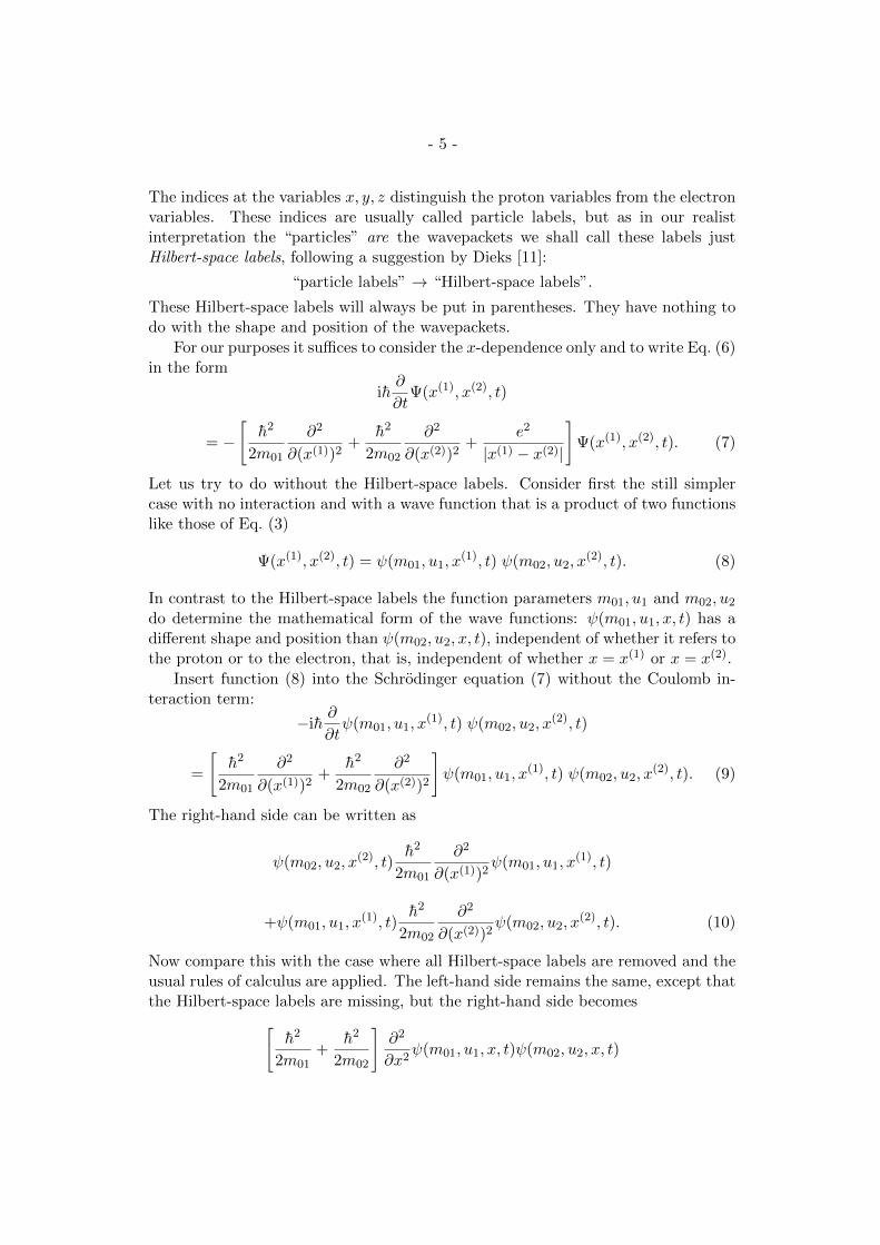
Now compare this with the case where all Hilbert-space labels are removed and theusual rules of calculus are applied. The left-hand side remains the same, except thatthe Hilbert-space labels are missing, but the right-hand side becomes[

h2

2m01+

h2

2m02

]∂2

∂x2ψ(m01, u1, x, t)ψ(m02, u2, x, t)

- 6 -

= ψ(m02, u2, x, t)

[h2

2m01+

h2

2m02

]∂2

∂x2ψ(m01, u1, x, t)

+ψ(m01, u1, x, t)

[h2

2m01+

h2

2m02

]∂2

∂x2ψ(m02, u2, x, t)

+2

[h2

2m01+

h2

2m02

](∂

∂xψ(m01, u1, x, t)

)(∂

∂xψ(m02, u2, x, t)

). (11)

This is different from (10) because each operator h2

2m0i

∂2

∂(x(i))2(i=1, 2) now operates

on both ψ(m01, u1, x, t) and ψ(m02, u2, x, t), that is, the operators operate no longeronly in their own associated Hilbert space but encroach the other Hilbert space too.So, simply removing the Hilbert-space labels does not work.

One might think of compensating the removal of the Hilbert-space labels by theintroduction of some other procedure. Indeed, in (10), in contrast to (11), the dif-ferential operator (repeated application of the momentum operator) containing theintrinsic parameter m01 operates only on the single-particle function which containsthe same parameter m01, and the same holds for operator and wave function withm02. Thus, we may indeed remove the Hilbert-space labels if we instead impose theexplicit prescription that the operators operate only on those wave functions whichhave the same intrinsic parameters.

Compared with putting Hilbert-space labels at the variables and straightfor-wardly applying the usual rules of calculus, such an extra prescription is a ratherclumsy procedure. It gets even clumsier if the interaction term in Eq. (7) is takeninto account, and still more so if the multi-particle wave function is no longer ofproduct form but is written as Ψ(x(1), x(2)) or just Ψ(1, 2). In this latter case thereare no longer any single-particle functions to be distinguished by means of intrinsicparameters. Of course, any multi-particle function can be expanded in a series ofproducts of single-particle functions, but working out the expansion coefficients maybe a laborious task, and putting Hilbert-space labels at the variables resolves theproblem is a much more convenient way.

Thus, in systems of non-identical particles we might in principle do withoutHilbert-space labels. These labels are only a convenient way of associating the single-particle operators with their respective single-particle wave functions. Operators andtheir associated wave functions must lie in the same Hilbert space. Note that weare here not concerned with endowing the physical quantum objects with additionalproperties, but only with constructing an appropriate formalism, a convenient book-keeping device.

Though the Hilbert-space labels have nothing to do with the mathematical formof the wavepackets it is

ψ(m01, u1, x(1), t) ψ(m02, u2, x

(2), t) 6≡ ψ(m01, u1, x(2), t) ψ(m02, u2, x

(1), t) (12)

because the Hilbert spaces of wavepacket 1 and wavepacket 2, though isomorphic,are different [7, p. 1378, formula (B-3)]. Indeed, going from the left-hand side of

- 7 -

formula (12) to the right-hand side is not innocuous because applying the Hamiltonoperator [in square brackets] of Eq. (9) would evidently lead to an expression thatis different from (10).

5 Self interactions

Another reason for introducing Hilbert-space labels is to exclude self interactions.In the realist interpretation [1], as well as in de Broglie’s conception of the wavefunction [12, p. 115, §50] the electron, say, is basically an extended cloud of electriccharge of density e|ψ(r, t)|2. In this conception it cannot a priori be excluded thatdifferent regions of the cloud interact with each other via Coulomb forces. Thatis, the usual Schrodinger equation for the hydrogen atom, for example, should becomplemented by an additional potential term of the form

ψ(r, t) e2∫ψ∗(r′, t)ψ(r′, t)

|r − r′|d3r′, (13)

where r and r′ denote different places within one and the same electron cloud.The Schrodinger equation with the additional term (13) is called the de Broglieequation by Tomonaga [12, p. 115, 315]. The term (13) has, however, to be omittedif the correct atomic energy levels are to be obtained. This was already noticed bySchrodinger in 1927 [13].

In quantum field theory the term (13) may be kept but has no effect because therethe fields (wave functions) are turned into operators, the operators are expressedby means of one-particle creation and annihiliation operators, and due to “normalordering” all annihilation operators operate first. In the term (13) two annihilationoperators operate on one and the same one-particle state. That means that thesecond annihilation operator operates on the vacuum state, and this annihilates theterm [12, p. 336 - 338], [14].

In the realist interpretation [1], which does not use concepts of relativistic quan-tum field theory, the exclusion of the term (13) is regarded as internal structureless-ness of the wavepacket, mentioned in Section 2.

The Hilbert-space labels allow us to distinguish terms which describe the inter-action between clouds representing different particles (cf. [7, p. 1426])∫

ϕ∗(r(1), t) η(r(2), t)

|r(1) − r(2)|d3r(1)d3r(2) (14)

from terms like (13), which describe the interaction between parts of one and thesame cloud, and to exclude these latter terms.

6 Relabelling and renaming

Relabelling, that is, permuting (exchanging, in the case of just two particles) theHilbert-space labels leads to a different physical situation, as we have pointed outwith formula (12). On the other hand, relabelling means giving the wave functionsother names, and physical description should be independent of the names chosen

- 8 -

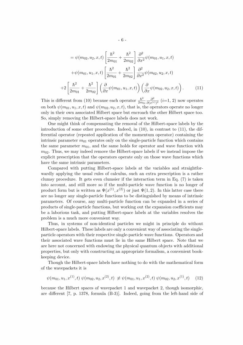
to denote the objects. In other words, physical description must be independent ofrenaming. What is the difference between relabelling and renaming?

In mathematical terms, leaving the physical description unchanged under re-labelling means that the Schrodinger equation and all expressions of physical sig-nificance must be permutation invariant. In quantum mechanics all expressions ofphysical significance can be expressed in terms of scalar products

(Ψ,Φ). (15)

In these products Φ may also be written as UΦ′ with U = unitary operator oftemporal evolution (=exp(−iHintt/h), e.g.). Ψ is taken at t = 0, but Φ′ at t < 0and by U is brought to t = 0.

The expectation value 〈A〉 = (Ψ, AΨ) can be expressed by scalar products inthe form 〈A〉 =

∑i λi|(ui,Ψ)|2, where λi and ui are the eigenvalues and eigenfunc-

tions, respectively, of the observable A. (ui,Ψ) can be taken as the amplitude of atransition from Ψ to ui in a reduction (“measurement”). The wave function ψ inthe localization (action) probability |ψ|2d3r, in particular, is taken as the amplitudeof a transition from Ψ into a normalizable superposition of position eigenfunctionsbelonging to continuous eigenvalues. We may summarize these cases by consideringthe scalar product

(Ψ, TΦ). (16)

Then, one requirement is that the product (16) must be permutation invariant underrenaming. As the permutation operator Pα is unitary (P †α = P−1

α ) the Pα invarianceof (16) is guaranteed if in addition to the wave function, the operator, too, is subjectto a transformation by means of Pα:

T → PαTP†α = PαTP

−1α and Ψ→ PαΨ, Φ→ PαΦ, so that

(Ψ, TΦ)→ (PαΨ, PαTP†αPαΦ) = (P †αPαΨ, TP †αPαΦ) = (Ψ, TΦ).

This is just like the unitary transformations effecting a change of the basis in Hilbertspace.

The transformation of both the operators and the wave functions also leaves theSchrodinger equation invariant:

ih∂

∂tΨ = HΨ → ih

∂

∂tPαΨ = PαHP

†αPαΨ = PαHΨ,

and multiplication from the left with P−1α yields

ihP−1α Pα

∂

∂tΨ = P−1

α PαHΨ so that we return to ih∂

∂tΨ = HΨ.

Thus, renaming means relabelling both the wave functions and the operators. Thisis not really surprising. Compare it with a police station which has a list containingthe names Ike and Mike. Ike is to be imprisoned, and Mike is to be given a reward.If Ike and Mike exchange their names each of them will receive quite a different

- 9 -

treatment, but if their names are exchanged in the police list, too, the situation willbe as before.

7 Identical particles. Basic features

Identical twins are two persons, but when we say that John William Strutt andLord Rayleigh are identical we mean that they are one and the same person. So, thefirst lesson is that the word “identical” has several distinct meanings. These maybe exemplified by pebbles, pingpong balls, and equal portions of water:

Pebbles can always be identified by their intrinsic properties such as size, mass,colour, shape and innumerable other properties revealed by more sophisticated meth-ods. We might not be interested in distinguishing them, or we might, in certainsituations, not be able to use more sophisticated methods (we may not be allowedto come sufficiently close) so that we cannot safely distinguish the pebbles, but inprinciple we always can.

Pingpong balls are equal in the sense that they all have the same intrinsic prop-erties. Imagine that you are shown two pingpong balls lying on the table, one onthe right-hand side and the other on the left-hand side. Then leave the room whilethe balls are moved by some other person. When you re-enter the room and see twoballs on the table at the previous positions you cannot say whether the balls havebeen exchanged or not. If you had stayed in the room you could have followed theirrespective trajectories and you would indeed know whether they are exchanged ornot. Of course, if you are allowed to use every method of testing the balls you willalways be able to discover intrinsic properties that are different in the two balls andcan be used to identify them. This is not meant here. The pingpong balls conceivedhere have the same intrinsic properties under every test.

Equal water portions cannot even be identified by means of their trajectories.Imagine a black and a white espresso cup, each filled with 40 cm3 of water. Pour thewater of both cups into a jar, and then fill a red and a green cup with the water ofthe jar, giving each cup again 40 cm3. In this case the question whether the waterportion which now is in the red cup has come from the black or from the white cupdoes not make sense. Pebbles and pingpong balls are impenetrable, water portionsare not.

Thus, pebbles can be identified by their intrinsic properties, pingpong balls bytheir trajectories, but equal water portions can only be identifided as long as theyare kept apart from each other: these are different kinds of indistinguishability.

Where are these objects met in the description of nature? Pebbles are certainlymet in classical (pre-quantum) mechanics of macroscopic objects. Whether ourpingpong balls are met in classical mechanics is a debated question (Section 12).The atoms of early kinetic theory are certainly serious candidates. The atoms ofquantum mechanics in their ground states may also be objects with the propertiesof our pingpong balls as long as they are localized at separate places as, for example,at the lattice sites of a crystal. Objects with the properties of our water portionsare met in quantum mechanics, where the objects are represented by wavepackets,which can overlap and condense (Sections 2, 13, 14).

- 10 -

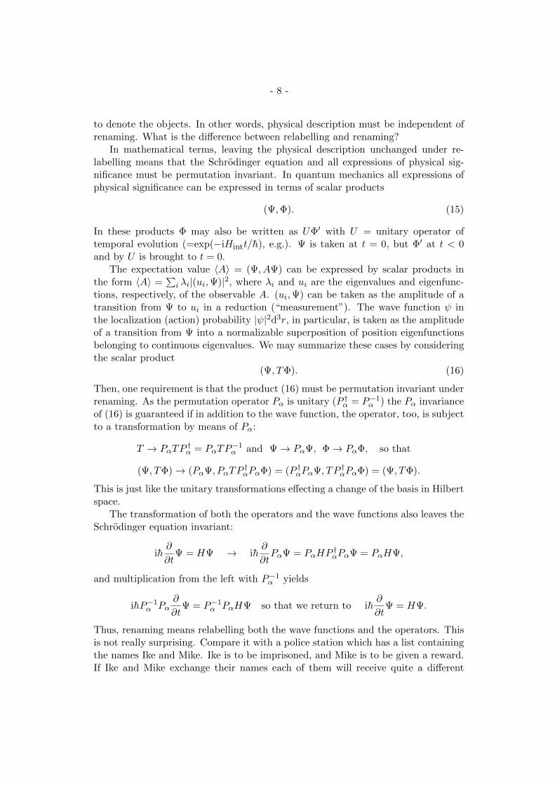
Let us now turn to the description of identical particles in quantum mechanics.Here the characteristic feature of treating systems of identical particles is that it isbased to a large extent on the treatment of non-identical particles: each wavepacketgets a Hilbert-space label.

In systems of non-identical particles the labels were in principle dispensablebecause their task could already be accomplished by the intrinsic parameters (massm0, charge e etc.). In systems of identical particles all intrinsic parameters are bydefinition equal, and now it is only the Hilbert-space labels at the variables x, y, zthat distinguish the particles in the formalism. Here the labels are not merely aconvenient but an indispensible book-keeping device allowing to associate the one-particle operators with their respective one-particle wave functions.

Thus, the Schrodinger equation for the two electrons in the helium atom reads[7, p. 1419], [9, p. 257], [10, p. 690, 774]

ih∂

∂tΨ =

2∑i=1

P 2i

2me−

2∑i=1

e2

|Ri|+

2∑i<j

e2

|Ri −Rj |

Ψ (17)

with

P 2i = −h2

(∂2

∂(x(i))2+

∂2

∂(y(i))2+

∂2

∂(z(i))2

). (18)

Ri is the vector pointing from the nucleus to a place in the cloud of electron i, andme is the electron mass. The wave function Ψ is antisymmetric

Ψ(x(1), x(2)) = −Ψ(x(2), x(1)). (19)

This property will be discussed in Section 11 below. For the present considerationthe interesting feature is that the indices i in Eq. (18) are Hilbert-space labels, andthat removing these labels from Eqs. (18) and (19) would lead to wrong physicalresults, much as in the case of the hydrogen atom considered in Section 4, Eqs. (9)and (11).

On the other hand, the labelling here introduces an ordering of the particles thathas no support in any intrinsic physical properties of the particles. One might wishthat in the description of systems of identical particles no ordinal numbers (numberof your bank account) should appear, but only cardinal numbers (balance of yourbank account), which specify how many particles belong to the system.

Indeed, a description of systems of identical particles, where only cardinal num-bers are involved is the occupation-number or Fock representation. Fermions andbosons in this representation are distinguished by the possible values of the occu-pation numbers: 0, 1 for fermions, and 0,...,∞ for bosons (elementary and n-foldcondensed wavepackets, in the language of [1]). But this remains an ad hoc postulateunless it is deduced from the more general assumptions of wave mechanics, whichlead to the Pauli exclusion principle and thus explain the occupation numbers.

Other approaches at getting along without Hilbert-space labels consist in workingfrom the outset with a configuration space where coordinates which result from

- 11 -

permutations do not define a new point [16], [15]. We do not discuss these approacheshere. The concern of the present note is only the usual text-book treatment ofidentical particles. In this treatment ordinal numbers, namely (Hilbert-space) labels,are introduced. But then, in order to remedy this, the ordering is neutralized by anadditional procedure: permuting the labels in every wave function, and adding allfunctions with the permuted labels (the “permutation” functions, for short) to theoriginal function. In this way we have labels and yet no ordering.

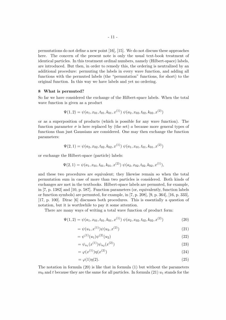
8 What is permuted?

So far we have considered the exchange of the Hilbert-space labels. When the totalwave function is given as a product

Ψ(1, 2) = ψ(a1, x01, t01, k01, x(1)) ψ(a2, x02, t02, k02, x

(2))

or as a superposition of products (which is possible for any wave function). Thefunction parameter σ is here replaced by (the set) a because more general types offunctions than just Gaussians are considered. One may then exchange the functionparameters:

Ψ(2, 1) = ψ(a2, x02, t02, k02, x(1)) ψ(a1, x01, t01, k01, x

(2))

or exchange the Hilbert-space (particle) labels:

Ψ(2, 1) = ψ(a1, x01, t01, k01, x(2)) ψ(a2, x02, t02, k02, x

(1)),

and these two procedures are equivalent; they likewise remain so when the totalpermutation sum in case of more than two particles is considered. Both kinds ofexchanges are met in the textbooks. Hilbert-space labels are permuted, for example,in [7, p. 1382] and [10, p. 587]. Function parameters (or, equivalently, function labelsor function symbols) are permuted, for example, in [7, p. 208], [9, p. 364], [16, p. 333],[17, p. 100]. Dirac [6] discusses both procedures. This is essentially a question ofnotation, but it is worthwhile to pay it some attention.

There are many ways of writing a total wave function of product form:

Ψ(1, 2) = ψ(a1, x01, t01, k01, x(1)) ψ(a2, x02, t02, k02, x

(2)) (20)

= ψ(u1, x(1))ψ(u2, x

(2)) (21)

= ψ(1)(u1)ψ(2)(u2) (22)

= ψu1(x(1))ψu2(x(2)) (23)

= ϕ(x(1))η(x(2)) (24)

= ϕ(1)η(2). (25)

The notation in formula (20) is like that in formula (1) but without the parametersm0 and t because they are the same for all particles. In formula (21) u1 stands for the

- 12 -

set a1, x01, t01, k01 of external parameters, which determine the shape and positionof the wavepacket, and the same for u2 (cf. formula (3) in Section 3). In formula(22) the variables x are suppressed and the Hilbert-space labels are put directly atthe function symbols. Formula (23) is like formula (4), and formula (24) like formula(5). Note that we may only exchange either the Hilbert-space labels or the functionparameters (labels, symbols). Exchanging both is the same as exchanging nothing.

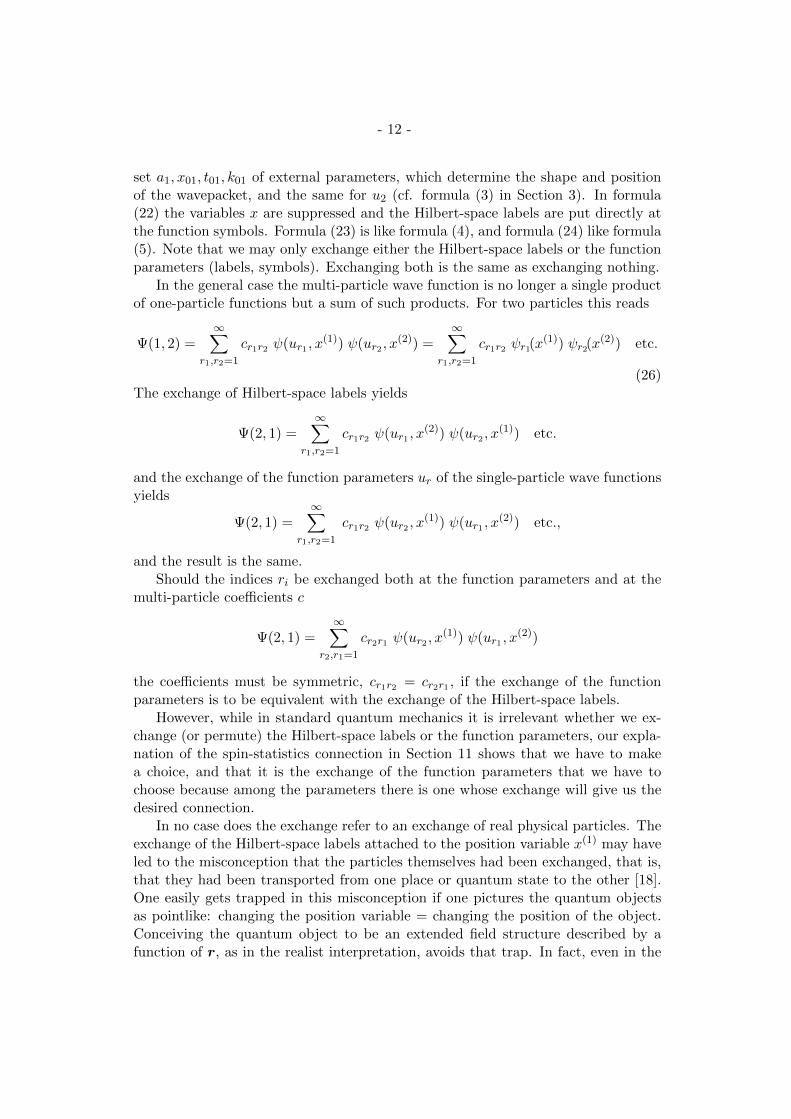
In the general case the multi-particle wave function is no longer a single productof one-particle functions but a sum of such products. For two particles this reads

Ψ(1, 2) =∞∑

r1,r2=1

cr1r2 ψ(ur1 , x(1)) ψ(ur2 , x

(2)) =∞∑

r1,r2=1

cr1r2 ψr1(x(1)) ψr2(x

(2)) etc.

(26)The exchange of Hilbert-space labels yields

Ψ(2, 1) =∞∑

r1,r2=1

cr1r2 ψ(ur1 , x(2)) ψ(ur2 , x

(1)) etc.

and the exchange of the function parameters ur of the single-particle wave functionsyields

Ψ(2, 1) =∞∑

r1,r2=1

cr1r2 ψ(ur2 , x(1)) ψ(ur1 , x

(2)) etc.,

and the result is the same.Should the indices ri be exchanged both at the function parameters and at the

multi-particle coefficients c

Ψ(2, 1) =∞∑

r2,r1=1

cr2r1 ψ(ur2 , x(1)) ψ(ur1 , x

(2))

the coefficients must be symmetric, cr1r2 = cr2r1 , if the exchange of the functionparameters is to be equivalent with the exchange of the Hilbert-space labels.

However, while in standard quantum mechanics it is irrelevant whether we ex-change (or permute) the Hilbert-space labels or the function parameters, our expla-nation of the spin-statistics connection in Section 11 shows that we have to makea choice, and that it is the exchange of the function parameters that we have tochoose because among the parameters there is one whose exchange will give us thedesired connection.

In no case does the exchange refer to an exchange of real physical particles. Theexchange of the Hilbert-space labels attached to the position variable x(1) may haveled to the misconception that the particles themselves had been exchanged, that is,that they had been transported from one place or quantum state to the other [18].One easily gets trapped in this misconception if one pictures the quantum objectsas pointlike: changing the position variable = changing the position of the object.Conceiving the quantum object to be an extended field structure described by afunction of r, as in the realist interpretation, avoids that trap. In fact, even in the

- 13 -

Copenhagen interpretation a particle shows up with a definite position only whenthe position is subject to measurement. Thus, though nowadays physical particletransportation is no longer taken seriously, the language used in even excellent text-books is still rather misleading [6], [7, p. 1377], [9, p. 364], [10, p. 585 - 588], [16,p. 335]. On the other hand, there are indeed books which conciously avoid speakingof particle exchange [19, p. 97], [20], [21].

The differing conceptions on the nature of the quantum object also have somebearing on the question of whether the spin component m of the quantum object isto be counted among the parameters or the variables of the wave function. In Pauli’sarticle [22] the spin component is counted among the variables. Pauli speaks of ex-change of spin co-ordinates, position co-ordinates, particles, and labels as equivalentprocedures, as is characteristic of the conception of point particles. The spin partof the wave function may be written as σµ(sz) = δµsz , where µ is a parameter ofthe wave function, namely an eigenvalue of the spin-component operator (≡ our m),and sz is the spin coordinate (cf. [17 p. 49, 50]). But the Kronecker delta meansthat the two have always the same value. Actually, what really counts is that thescalar product satisfies (σµ(sz), σµ′(sz)) = δµµ′ . The spin coordinate sz serves onlyas a summation index when forming the scalar product in a special way.

In our conception the spin component m is to be counted among the externalparameters of the wave function.

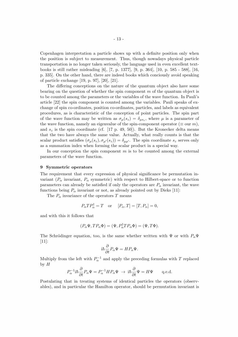
9 Symmetric operators

The requirement that every expression of physical significance be permutation in-variant (Pα invariant, Pα symmetric) with respect to Hilbert-space or to functionparameters can already be satisfied if only the operators are Pα invariant, the wavefunctions being Pα invariant or not, as already pointed out by Dieks [11]:

The Pα invariance of the operators T means

PαTP†α = T or [Pα, T ] = [T, Pα] = 0,

and with this it follows that

(PαΨ, TPαΦ) = (Ψ, P †αTPαΦ) = (Ψ, TΦ).

The Schrodinger equation, too, is the same whether written with Ψ or with PαΨ[11]:

ih∂

∂tPαΨ = HPαΨ.

Multiply from the left with P−1α and apply the preceding formulas with T replaced

by H

P−1α ih

∂

∂tPαΨ = P−1

α HPαΨ → ih∂

∂tΨ = HΨ q.e.d.

Postulating that in treating systems of identical particles the operators (observ-ables), and in particular the Hamilton operator, should be permutation invariant is

- 14 -

reasonable, as it is essentially the permutation invariance of the Hamilton functionof classical meachanics.

Nevertheless, in spite of the fact that with Pα symmetric operators the Schrodingerequation and every expression of physical significance is already Pα symmetric, cur-rent quantum mechanics postulates that the wave functions, too, be Pα symmetric.Why?

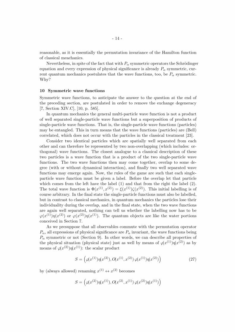
10 Symmetric wave functions

Symmetric wave functions, to anticipate the answer to the question at the end ofthe preceding section, are postulated in order to remove the exchange degeneracy[7, Section XIV.C], [10, p. 585].

In quantum mechanics the general multi-particle wave function is not a productof well separated single-particle wave functions but a superposition of products ofsingle-particle wave functions. That is, the single-particle wave functions (particles)may be entangled. This in turn means that the wave functions (particles) are (Bell)correlated, which does not occur with the particles in the classical treatment [23].

Consider two identical particles which are spatially well separated from eachother and can therefore be represented by two non-overlapping (which includes: or-thogonal) wave functions. The closest analogue to a classical description of thesetwo particles is a wave function that is a product of the two single-particle wavefunctions. The two wave functions then may come together, overlap to some de-gree (with or without dynamical interaction), and finally two well separated wavefunctions may emerge again. Now, the rules of the game are such that each single-particle wave function must be given a label. Before the overlap let that particlewhich comes from the left have the label (1) and that from the right the label (2).The total wave function is Φ(x(1), x(2)) = ξ(x(1))ζ(x(2)). This initial labelling is ofcourse arbitrary. In the final state the single-particle functions must also be labelled,but in contrast to classical mechanics, in quantum mechanics the particles lose theirindividuality during the overlap, and in the final state, when the two wave functionsare again well separated, nothing can tell us whether the labelling now has to beϕ(x(1))η(x(2)) or ϕ(x(2))η(x(1)). The quantum objects are like the water portionsconceived in Section 7.

As we presuppose that all observables commute with the permutation operatorPα, all expressions of physical significance are Pα invariant, the wave functions beingPα symmetric or not (Section 9). In other words, we can describe all properties ofthe physical situation (physical state) just as well by means of ϕ(x(1))η(x(2)) as bymeans of ϕ(x(2))η(x(1)): the scalar product

S =(ϕ(x(1))η(x(2)), O(x(1), x(2))ϕ(x(1))η(x(2))

)(27)

by (always allowed) renaming x(1) ↔ x(2) becomes

S =(ϕ(x(2))η(x(1)), O(x(2), x(1))ϕ(x(2))η(x(1))

)

- 15 -

and by the symmetry O(x(2), x(1)) = O(x(1), x(2)) this becomes

S =(ϕ(x(2))η(x(1)), O(x(1), x(2))ϕ(x(2))η(x(1))

),

and this is just the scalar product (27) with the exchange function ϕ(x(2))η(x(1))instead of the original function ϕ(x(1))η(x(2)).

The general superposition principle then demands that the physical situation isdescribed just as well by the superposition

Ψ = α ϕ(x(1)) η(x(2)) + β ϕ(x(2)) η(x(1)) (28)

with|α|2 + |β|2 = 1. (29)

Although the Hilbert-space labels have nothing to do with the mathematical formof the wavepackets, Eq. (28) is not merely the superposition of two equal functions.The reason is that only the Hilbert-space labels are exchanged but not the functionparameters (cf. (23), (24)). The operator operating on the variables x(1) meets adifferent function in the first than in the second term of the sum.

Eq. (28) represents the well known exchange degeneracy [7, p. 1375 - 1377],[9, p. 365], [10, p. 583]. Physical predictions may now depend on the values of αand β. This is due to interference between the α and β terms when expressions ofphysical significance are constructed which involve the superposition (28). To seethis consider the scalar product(

[αϕ(x(1))η(x(2)) + β ϕ(x(2))η(x(1))], O(x(1), x(2))[αϕ(x(1))η(x(2)) + β ϕ(x(2))η(x(1))])

(30)which by renaming and using the symmetry of O becomes

=(αϕ(x(1))η(x(2)), Oαϕ(x(1))η(x(2))

)+(αϕ(x(1))η(x(2)), Oβ ϕ(x(2))η(x(1))

)+(β ϕ(x(2))η(x(1)), Oαϕ(x(1))η(x(2))

)+(β ϕ(x(2))η(x(1)), Oβ ϕ(x(2))η(x(1))

)= (|α|2 + |β|2)

(ϕ(x(1))η(x(2)), Oϕ(x(1))η(x(2))

)+(α∗β + β∗α)

(ϕ(x(1))η(x(2)), Oϕ(x(2))η(x(1))

), (31)

where (|α|2 + |β|2) = 1, but (α∗β + β∗α) = 2Re{α∗β}.In order to get definite predictions (scalar products) the values of α and β have

to be fixed. As there are no a priori physical arguments in sight, this is done by wayof a postulate. Of course, a basic requirement for the postulate is that it must leadto predictions that are confirmed by experiment. A postulate which succeeds in thisand which fits well into the general symmetry requirements in systems of identicalparticles is

α = β =1√2

(32)

- 16 -

resulting in a symmetric wave function (28), that is, a function that is invariantunder the exchange of the Hilbert-space labels (1), (2) or the function parametersor the function symbols ϕ, η.

Actually in traditional quantum mechanics the postulate is not (32) but rather

±α = β =1√2. (33)

This will be discussed in the next section.In the current formalism the total wave function of a system of identical particles

is always assumed to be a superposition like (28) with (32) or (33). This amountsto assuming that the considered wave functions at some time in the past have over-lapped and the entanglement thereby established has persisted. This has not ledto any observed contradictions. Even if a superposition is formed both before andafter the overlap this makes no difference to forming the superposition only before(or only after) the overlap because the symmetrizer S =

∑α Pα (and also the an-

tisymmetrizer∑α εαPα) is a Hermitian projection operator (no longer unitary), so

that (cf. [7, p. 1380])

(SΨ, SΦ) = (S†SΨ,Φ) = (S2Ψ,Φ) = (SΨ,Φ).

Only when there are explicit physical reasons to assume that the considered particlesare independent (one particle being produced in the Andromeda galaxy and the otherin our Milky-Way galaxy, say) the total wave function is taken as a simple productof one-particle wave functions.

Sometimes one finds the following “proof” of relation (33): the identity of theparticles implies that the original and the exchange wave function must be essentiallythe same, that is, they can at most differ by a constant factor λ: Ψ(2, 1) = λΨ(1, 2).Combining this with the defining equation of the permutation operator, Ψ(2, 1) =PαΨ(1, 2), we get PαΨ(1, 2) = λΨ(1, 2) so that Ψ(1, 2) must be an eigenfunction ofPα. As (for any two particles) P 2

α = 1 the eigenvalues of Pα are ±1, so λ = ±1. Thisis no proof but merely a different postulate because it is based on a requirementimposed directly on the Ψ function, which in itself is no expression of direct physicalsignificance.

11 Antisymmetric wave functions

As described in Section 10, in conventional quantum mechanics the postulate forremoving the exchange degeneracy is not Eq. (32) but Eq. (33), thus admittingsymmetric and antisymmetric wave functions. The justification for the two signsin Eq. (33) in conventional quantum mechanics is based on the observation that ifthe wave function Ψ is a solution of the Schrodinger equation with Pα-symmetricHamilton operator, then PαΨ is also a solution (cf. Section 9). Ψ can then be writtenas a linear combination of functions grouped into systems that transform accordingto particular irreducible representations of the permutation group. The postulate(33) then is equivalent to the postulate that only the two representations of degree

- 17 -

(dimension) 1 are relevant for the description of nature [10, p. 1117], [22]. The wavefunction (28) with the plus sign from Eq. (33), meaning bosons, is empirically foundto represent particles with integral spin, in units of h, and the function with theminus sign, meaning fermions, is found to represent particles with half-integral (i.e.half-odd-integral) spin. This connection between spin and statistics was first provedby Fierz and by Pauli in the framework of relativistic quantum field theory [24]. Inthe last 20 years a rising number of papers with a peak statistical frequency in 2004have appeared which tried to prove such a spin-statistics connection under varioussets of conditions, in particular within the framework of quantum mechnics.

I will here describe my own proposal [25]. It follows the suggestion by Feynman[26], that the exchange degeneracy is fixed by Eq. (32), that is, by the plus signonly. The minus sign arises in the construction of the exchange function from theoriginal function. The single-particle wave functions are of course complemented bya spin part. The spin-component eigenfunctions depend on the quantum numberm and on the azimuthal angle χ of a rotation about the spin-quantization axis inthe form exp(imχ). This is standard quantum mechanics [7, p. 703, 984, 985]. Instandard quantum mechanics the angle χ is however considered to have no physicalsignificance, and is usually neglected. In my approach the external parameter χ isexchanged along with the other parameters, and thereby acquires physical signifi-cance because it becomes a relative phase angle. In the case of half-integral m foreach value of χ there are two eigenfunctions, which differ by their signs. This is thewell known spinor ambiguity, and like the ambiguity represented by the exchangedegeneracy, it has also to be fixed. This is done by effecting the exchange of χby way of rotation, and admitting only rotations in one sense, either clockwise orcounterclockwise. If it is done so, the second term on the right-hand side of Eq. (28)acquires the factor (−1)2s, hs being the total spin of the particle.

The essential step leading to this result can be outlined in a simple example: startfrom the special function ψ(1)(ua, χa)ψ

(2)(ub, χb), where both single-particlefunctions belong to the same m, and χb > χa. The exchange of the parame-ters ua and ub changes the function into ψ(1)(ub, χa)ψ

(2)(ua, χb). Then, whenψ(1)(ub, χa) is rotated counterclockwise from χa to χb we have ψ(1)(ub, χb) =exp(im(χb − χa))ψ(1)(ub, χa). Likewise, when ψ(2)(ua, χb) is rotated counter-clockwise from χb to χa we have ψ(2)(ua, χa) = exp(im(2π+χa−χb))ψ(2)(ua, χb).In this way the product ψ(1)(ub, χa)ψ

(2)(ua, χb) becomes F×ψ(1)(ub, χb)ψ(2)(ua, χa),

where

F = exp(−im(χb − χa)) exp(−im(2π + χa − χb)) = (−1)2m = (−1)2s. (34)

It is seen that this result can only be obtained when the function parameters,not the Hilbert-space labels, are exchanged. Exchange of function parameters andexchange of Hilbert-space labels are here not equivalent. For the described procedurethe multi-particle wave function Ψ(1, 2, . . . , N) must be given in terms of one-particlefunctions, but this is in principle always possible (cf. Eq. (26) in Section 8).

The result (37) also holds for functions of general form, for any number of par-ticles, and in the relativistic domain. The connection between spin and statistics is

- 18 -

thus changed from an axiom into a theorem, revealing a larger domain of phenom-ena which good old quantum mechanics can incorporate into a coherent theoreticalpicture. The antisymmetric wave functions do not emerge from the permutationgroup with its two inequivalent one-dimensional representations, but from the rota-tion group with the ambiguity of its spinor representation. This entails that onlyBose and Fermi statistics, but no parastatistics result.

The antisymmetric wave functions lead to the Pauli exclusion principle, whichmay be formulated by saying that “no antisymmetric wavefunction describing anN-electron atom can be made up of one-electron functions, two of which have thesame set of one-electron quantum numbers” [17, p. 101]. Or: no antisymmetricwave function exists which could describe two fermions represented by two equalone-particle wave functions (cf. [7, p. 1389]).

12 The term −k lnN ! in the entropy

We will now consider some implications of the preceding considerations for statisticalmechanics. Either term on the right-hand side of formula (28) is a product of single-particle wave functions and is thus the closest quantum mechanical analogue to aclassical situation: the first term would mean that particle 1 is in phase-space regiona and particle 2 in region b, whereas the second term would mean the reverse. Inclassical statistical mechanics these two states are considered as different. In otherwords, exchanging the particles leads to a new classical state. In quantum mechanicsthere is only one state, given by formula (28), and with the choice (32) or (33) of thecoefficients α and β the exchange of Hilbert-space labels does not lead to a new state.In the case of N identical particles there are N ! possible classical states, accordingto the number of possible permutations of N elements, but still only one quantummechanical state. In other words, when going from classsical to quantum mechanicsthe number of states has to be divided by N ! This is a justification of the well-known subtraction of the term k lnN ! in the entropy formula of classical statisticalmechanics in order to resolve the Gibbs paradox concerning the entropy of mixing[19, p. 193], [27, p. 141], [28]. Notice that this holds independently of whether (32)or (33) is chosen, that is, independent of whether the quantum mechanical statesare symmetric or antisymmetric, i.e. describe bosons or fermions.

Whether quantum mechanics is really necessary for the justification of the divi-sion by N ! is a debated question [19, p. 96], [29]. It depends on whether or not onecounts the pingpong balls of Section 7 among the classical objects. If one attributesthe properties of our pingpong balls to the classical particles, it is true that thevarious ways of filling or refilling the sites with particles can be distinguished, butwhen only the resulting arrangement is seen it is no longer possible to distinguishthe various ways that have led to it. The entropy is a function of state, that is,it depends only on the resulting arrangement and not on its past history. Thendivision by N ! makes already sense in classical statistical mechanics.

13 Bose, Fermi and Boltzmann probabilities

The essential new feature of quantum as compared to classical particles is that there

- 19 -

are situations where quantum particles cannot even be identified by their position.This happens when there is, at some time, some overlap of the wavepackets whichrepresent the particles. In particular, in quantum mechanics it can happen thattwo or n single-particle wave functions after the overlap are equal. This, in therealist language of [1], means n-fold condensed wavepackets, and in the language ofstatistical mechanics it means a multiple occupation of quantum phase-space cells ofsize h3. The objects within such a quantum cell can no longer be distinguished by anymeans, and permutation of them does not even make sense. They are comparableto water portions in a jar.

In the Fermi case a total wave function with two or more single-particle wavefunctions being equal is excluded by the appearance of the minus sign in formula(33), leading to the Pauli exclusion principle. Accordingly, never more than twoequal fermions can be in one quantum cell, and it might seem that there is neverany overlap between fermion functions, so that fermions are like pebbles and notlike water portions. However, this refers to the situation after the process of en-tanglement. Before this process had set in, there has been overlap because thegeneral single-particle wave function is a superposition of several spin-componenteigenfunctions. It is easy to convince oneself that the scalar product between suchsuperpositions is nonzero (they are not orthogonal), and that the nonzero termsexhibit spatial overlap between one-particle functions which have the same spincomponent. Only if the total state initially is a single product of one-particle func-tions, and the spin components are all different, can the particles be considered aseffectively distinguishable, i.e., as pebbles (cf. [25, Section 7]).

Classical statistical mechanics considers the division of phase space into distin-guishable regions (energy regions, cells, groups, levels, shells etc. in the varioustextbooks) but does not consider the subdivision of the chosen regions into quan-tum cells of size h3 (subcells, compartments, quantum states etc.). In quantummechanics this subdivision is instrumental in determining the probability wi of hav-ing ni particles in a region i comprising gi quantum cells and leads to the well-knownformulas for bosons

wi =(ni + gi − 1)!

ni!(gi − 1)!=

(ni + gi − 1

ni

)=

(ni + gi − 1gi − 1

)(35)

and for fermions

wi =gi!

ni!(gi − ni)!=

(gini

). (36)

As stated above, permutation of the particles within one quantum cell does notmake sense and so should not even be mentioned. Actually, the expression ni!,which means permutation of all particles in region i, even those that might be inone and the same quantum cell, appears in both formulas. But this is only so inthe mathematical formula and does not appear in the definition of the wi: in theFermi case wi is defined as the number of ways in which ni quantum cells can bechosen from gi distinguished quantum cells into which the ni particles can be put.

- 20 -

In the Bose case wi is defined as the number of ways in which the number ni can bedecomposed into the sum of gi nonnegative integers, namely the respective numberof particles put in each of the quantum cells [19, p. 70, 100].

In the limit ni � gi the Bose and the Fermi formulas tend to

gnii

ni

(1± ni(ni − 1)

2gi

), (37)

where the upper sign refers to bosons and the lower sign to fermions. In the Bosecase formula (40) can be obtained by writing

(ni + gi − 1)!

ni!(gi − 1)!=gnii

ni!(1 + 1/gi) (1 + 2/gi) · · · (1 + (ni − 1)/gi)

and neglecting all terms of second and higher order in (1/gi) when evaluating theproduct. The Fermi case obtains in an analogous way.

Thus in the limit ni/gi → 0 both the Bose and the Fermi formula tend to

wi =gnii

ni!, (38)

which may be called the correct Boltzmann formula [27, p. 182]. The limit ni/gi → 0means that there are many more quantum cells than particles in region i, so thatthe probability of two or more particles occupying the same quantum cell becomeszero. This is the classical limit because in this limit the size h3 of a quantum cellgoes to zero and the number gi of quantum calls in the region i goes to infinity.

The approach from the quantum to the classical case can also be seen fromthe superposition (28) when it is generalized to comprise sums of products of none-particle wave functions

Ψ =g∑

r1,r2,···,rn=1

cr1r2···rN ψr1(x(1)) ψr2(x(2)) · · ·ψrn(x(n)), (39)

where the symmetry type of the coefficients may be left open. n is the number ofactually present wavepackets (particles), g is the (maximum) number of formallypossible elementary (one-quantum) wavepackets in the chosen energy interval.

The sum (42) has gn terms. The number of terms which have all indices different

is

(gn

)n!, namely the number

(gn

)of possibilities of choosing n different values

out of the g (≥ n) possible values of the indices times the number n! of permutationsof the n chosen values among themselves. The fraction of terms with two or moreequal indices is therefore

1− g!

(g − n)!gn→ n(n− 1)

2g→ 0 (40)

when g → ∞, n fixed. This can be seen by a consideration like that leading toformula (40).

- 21 -

Thus, whatever the values of the coefficients cr1r2···rn in the terms with twoor more equal indices, the contribution of these terms to the sum (42) sinks intoinsignificance compared with the overwhelming number of the other terms whenn/g → 0. This is independent of whether Ψ in (42) is symmetrized or not becausethe described considerations would apply to each of the terms with permuted labelsin the symmetrized Ψ.

14 The Bose and Fermi distributions

By Bose and Fermi distributions I mean

Ndp =gp

exp[(ε− µ)/kT ]± 1, (41)

where Ndp means, in the usual interpretation, the time averaged number of particlesin some volume V whose absolute value of momentum lies in the interval dp aboutp. µ is the chemical potential. gp = 4πV p2dp/h3, and ε = [p2c2 + (mc2)2]1/2

is the total energy of a particle. The distributions (44) can be obtained from theformulas (38) and (39) through the well known procedure of maximizing the entropyS = k ln

∏iwi.

I would like to mention here that the distributions can also be obtained by con-sidering n-fold condensed wavepackets (wavepackets representing n quanta) as thefundamental units of an ideal gas. gp is then the maximum possible number ofwavepackets in V covering the momentum interval dp. The packets can be treatedas statistically independent objects, whereas the quanta, if we were to take these asentities of their own, are not independent. Actually, what in the usual interpretationof formula (44) is the number of particles, is in the realist interpretation the numberof quanta. For when a wavepacket causes an effect, a response of a counting appa-ratus say, this is usually interpreted as the count of a particle. Thus the statisticalinterdependence of the quanta shows up as the “mutual influence of the moleculeswhich for the time being is of a quite mysterious nature” [23]. The wavepacketscan condense, decondense, and exchange energy among themselves. This leads toa simple and symmetric balance equation, following Einstein’s method of emissionand absorption of radiation by atoms [30]:

p(s, εi1)p(r, εf

1)q(s′, εi2)q(r′, εf

2) = p(s−n, εi1)p(r+n, εf

1)q(s′−n′, εi2)q(r′+n′, εf

2). (42)

Two kinds of wavepackets are considered (Einstein: atoms and photons). p(s, εi1)dεi

1

is the mean number of s-fold condensed packets of kind 1 in volume V that represents quanta in the energy interval dε[= (∂ε/∂p)dp], and analogously with the otherterms. q( ) refers to packets of kind 2. The solution of Eq. (45), when energyconservation in the form n(εi

1 − εf1) = n′(εf

2 − εi2) is taken into account, is

p(s, ε) = a(ε) exp[−(bε− c)s] (43)

q(s, ε) = a′(ε) exp[−(bε− c′)s], (44)

- 22 -

where b = 1/kT, c = µ/kT, c′ = µ′/kT follow from thermodynamic relations involv-ing the entropy

S = k ln∏{dεi}

gp!

[p(0, εi)dεi]! [p(1, εi)dεi]! · · ·. (45)

Then, when observing that∑{s} p(s, ε)dε = gp and that for Bose packets the num-

bers s, r etc. in Eqs. (45) to (47) are nonnetative integers, while for Fermions theycan only be 0 or 1, the total number of quanta

Ndp =∑{s}

sp(s, ε)dε

is given by the formulas (44). And as I have said, these quanta, not the wavepackets,are identified with the particles in the usual interpretation of formula (44). The usualfluctuation formulas for quantum counts can be obtained on the same line.

References

[1] Jabs, A.: Quantum mechanics in terms of realism, arXiv:quant-ph/9606017

[2] Jabs, A.: An Interpretation of the Formalism of Quantum Mechanics in Termsof Epistemological Realism, arXiv:1212.4687 (Brit. J. Philos Sci. 43, 405 -421 (1992))

[3] Piaget, J.: The Construction of Reality in the Child (Routledge & Kegan Paul,London, 1954, translation from the French) p. 4

[4] Glasersfeld, E. von: Radical Constructivism. A Way of Knowing and Learn-ing (The Falmer Press, London, 1995); Foerster, H. von: Observing Systems(Intersystems Publications, Seaside CA, 1982)

[5] Andersen, H.C.: The Emperor’s New Clothes, http://www.andersen.sdu.dk/vaerk/hersholt/TheEmperorsNewClothes e.html (J. Hersholt, The CompleteAndersen (The Limited Editions, New Club, New York, 1949, translation fromthe Danish)). – And what did the emperor and his noblemen do after the wholetown joined in the child’s words? “So, he walked more proudly than ever, ashis noblemen held high the train that wasn’t there at all”

[6] Dirac, P.A.M.: The Principles of Quantum Mechanics (Oxford UniversityPress, London, 1967) p. 207, 217, 218

[7] Cohen-Tannoudji, C., Diu, B., Laloe, F.: Quantum Mechanics, Vols. I, II(John Wiley & Sons, New York, 1977, translation from the French)

[8] Wohl, C.G., et al.: Review of Particle Properties, Rev. Mod Phys. 56 (2),Part II (1984)

[9] Schiff, L.I.: Quantum Mechanics (McGraw-Hill, New York, 1968)

- 23 -

[10] Messiah, A.: Quantum Mechanics, Vols. 1, 2 (North-Holland, Amsterdam,1970, 1972, translation from the French)

[11] Dieks, D.: Quantum Statistics, Identical Particles and Correlations, Synthese82, 127 - 155 (1990)

[12] Tomonaga, S.-I.: Quantum Mechanics, Vol. II (North-Holland PublishingCompany, Amsterdam, 1966, translation from the Japanese)

[13] Schrodinger, E.: Annalen der Physik (Leipzig) 82 (4), 265 - 273 (1927). En-glish translation in: Collected Papers on Wave Mechanics (Chelsea PublishingCompany, New York, 1982) p. 136

[14] Doring, W.: Atomphysik und Quantenmechanik, Vol. II (de Gruyter, Berlin,1976) p. 402

[15] Laidlaw, M.G.C., DeWitt, C.M.: Feynman Functional integrals for Systems ofIndistinguishable Particles, Phys. Rev. D 3 (6), 1375 - 1378 (1971); Nelson,E.: Quantum Fluctuations (Princeton University Press, Princeton, 1985) p.100 - 102; Leinaas, J.M., Myrheim, J.: On the Theory of Identical Particles,Nuovo Cimento 37B (1), 1 - 23 (1977)

[16] Gottfried, K.: Quantum Mechanics (Benjamin, Reading MA, 1966)

[17] Cowan, R.D.: The Theory of Atomic Structure and Spectra (University ofCalifornia Press, Berkeley, 1981)

[18] Heisenberg, W.: Mehrkorperproblem und Resonanz in der Quantenmechanik,Z. Phys. 38, 411 - 426 (1926), especially p. 421

[19] Ter Haar, D.: Elements of Thermostatistics (Holt, Rinehart and Winston,New York, 1966)

[20] Peres, A.: Quantum Theory: Concepts and Methods (Kluwer, Dordrecht, 1993)p. 126

[21] Davydov, A.S.: Quantum Mechanics, 2nd edition (Pergamon Press, Oxford,1976, translation from the Russian) p. 306

[22] Pauli, W.: Die allgemeinen Prinzipien der Wellenmechanik, in: Handbuchder Physik, Vol. 24, Part I, edited by Geiger, H., Scheel, K. (Springer-Verlag, Berlin, 1933) Chapter 2, Number 14. English translation of a 1958reprint: General Principles of Quantum Mechanics (Springer-Verlag, Berlin,1980) Chapter VII, Section 14(a)

[23] Einstein, A.: Quantentheorie des idealen einatomigen Gases, Zweite Ab-handlung, Sitzungsberichte der Preußischen Akademie der Wissenschaften,Physikalisch-Mathematische Klasse, Berlin, 1925, p. 3 - 14

- 24 -

[24] Fierz, M.: Uber die relativistische Theorie kraftefreier Teilchen mit beliebigemSpin, Helv. Phys. Act. 12, 3 - 37 (1939); W. Pauli, The connection betweenspin and statistics, Phys. Rev. 58, 716 - 722 (1940)

[25] Jabs, A.: Connecting spin and statistics in quantum mechanics, arXiv:0810.2399

[26] Feynman, R.P.: The reason for antiparticles, in: Elementary Particles and theLaws of Physics, edited by Feynman, R.P., Weinberg, S. (Cambridge Univer-sity Press, New York, 1987) p. 1 - 59, especially p. 56 - 59

[27] Huang, K.: Statistical Mechanics, 2nd edition (John Wiley & Sons, New York,1987)

[28] Becker, R.: Theorie der Warme (Springer-Verlag, Berlin, 1961) p. 24, 25, 117,118. English translation: Theory of Heat (Springer-Verlag, Berlin, 1967) p. 26,134, 135

[29] Saunders, S.: On the Explanation for Quantum Statistics, arXiv:quant-ph/0511136 (Studies in the History and Philosophy of Modern Physics 37,192 - 211 (2006))

[30] Einstein, A.: Zur Quantentheorie der Strahlung, Physik. Zeitschr. 18, 121 -128 (1917). English translation in: Ter Haar, D.: The old quantum theory(Pergamon Press, Oxford, 1967)

——————————