A REAL-TIME MOTION PLANNING ALGORITHM FOR AHYPER-REDUNDANT SET OF MECHANISMS

ODED MEDINA, BOAZ BEN MOSHE, AND NIR SHVALB

ABSTRACT. We introduce a novel probabilistic algorithm (CPRM)for real-time motion planning in the configuration space C. Ouralgorithm differs from a Probabilistic Road Map algorithm (PRM)in the motion between a pair of anchoring points (local planner)which takes place on the boundary of the obstacle subspace O.We define a varying potential field f on ∂O as a Morse functionand follow ~∇f . We then exemplify our algorithm on a redundantworm climbing robot with n degrees of freedom and compare ouralgorithm running results with those of PRM.

1. INTRODUCTION

Hyper-redundant robots are characterized by considerable kine-matic redundancy (see [1], [2]). Hyper-redundant robots can be di-vided into the following groups:(1) Robot Swarms: coordinated multi-robot systems which consistof large numbers of mostly simple physical robots. Each swarmmember may be restricted to motion on a given graph or may befree to translate in space. Potential applications for swarm robotsare mainly for sensing tasks, where miniaturization is essential. Aswarm, with each member possessing few degrees of freedom, caneasily give rise to an entity with hundreds of degrees of freedom(see [3]). (2) Snake Robots: biomorphic hyper-redundant robots thatresemble a snake. Their ability to change the shape of their bodiesallows them to perform a wide range of behaviors, such as climb-ing stairs or tree trunks. Their extra joints enhance maneuverabilitywithin tight obstacle fields, suggesting applications in congested en-vironments (disaster relief [4], medical applications [5] etc.). Rigid-link hyper-redundant designs imitate the biological backbone andmay possess many degrees of freedom (for example consider [6],featuring 4 DOF’s, and the Surgical Snake-like Robot [7]). (3) hu-manoid robots: are robots which resemble the human body, and may

Date: August 10, 2011.1

also present with dozens of DOF’s. (see [8]).Due to their great deal of redundancy it is easier to control thesemechanisms by a predefined set of motions rather than calculatetheir options in real-time. However, if they are to be deployed nearan obstacle lade zone, though mechanically fit, they would need areal-time computing algorithm for problem solving on the go. Inthis paper we present our algorithm for this problem and exemplifyour algorithm on such a robot.

1.1. Defintion. In a a mechanism, configuration space C is the set of all itspossible configurations.1.2. Defintion. In a given mechanism, its free configuration space Cfreeand a pair of configurations ps, pg ∈ Cfree, motion planning is an algo-rithm that finds a path γ ∈ Cfree from ps to pg. An optimal path is onewhich minimizes a weight function(s) defined on Cfree.It is also possible to set W - a certain submanifold of Cfree to be the sub-manifold on which motion planning will take place (i.e. instead of of Cfree)see [9]. Note that in order to take advantage of the redundancy (overcomingobstacles) for hyper-redundant robots we require that W = Cfree.

Various algorithms exist for motion planning [10]. Grid-based ap-proaches overlay a grid on top of the configuration space, and as-sume each configuration is identified with a grid point. At eachgrid point, the robot is allowed to move to adjacent points as longas the line between them is entirely within the Cfree. This discretizesthe set of actions, and search algorithms, like A?, Dijkstra etc., areused to find a path from the beginning point to the goal. Still, theabove mentioned example of hyper-redundant robots shows thatthese give rise to astronomical configuration spaces and hence arenot applicable for real-time computation. The following algorithmsare commonly used for real-time computations: (1) Potential fieldalgorithms place focal points of repulsion and attraction within theconfiguration space, such that the resultant field reflects the valuesof a certain weight function. A path may then be constructed fromthe point of origin, subject to the direction of the potential field, tothe destination. Such potential field algorithms are efficient, but fallprey to local minima (see [11]), and when applying such algorithmsto a obstacle congested environment local minima are abundant. Yetpotential field algorithms may be used as a local planner [12]. (2)Sampling-based algorithms represent the configuration space with aroadmap of sampled configurations. A basic algorithm samples Nconfigurations in C, and retains those in Cfree to use as milestones. Aroadmap is then constructed, connecting all milestone pairs p and q

2

if the line segment pq is entirely within Cfree. These algorithms workwell for high-dimensional configuration spaces, because unlike com-binatorial algorithms, their running time is not (explicitly) exponen-tially dependent on the dimension of C, and in general they are sub-stantially easier to implement. They are probabilistically complete,i.e. the probability that they will produce a solution approaches 1as runtime increases [13]. However, they are not applicable for real-time computations when considering the hyper-redundant case (see[14] for exactly the same problem as exemplified here).

This paper addresses the problem of real-time motion planning forthe hyper-redundant robot by combining the two algorithms.

1.3. Remark. In order to tackle the elapsed time problem one may al-ternatively attempt not to optimize the motion planning algorithms,but to simplify the configuration spaceIn other words, it is possibleto reduce the configuration space by severe compression (see Med-ina et.al. [15]) so that a robot’s embedded motion planning systemwill be capable of storing and accessing an otherwise immense datafile, far beyond the system’s memory capacity. This issue, however,is beyond the scope of this paper.

2. THE MECHANICAL SYSTEM

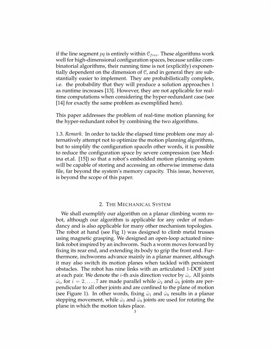
We shall exemplify our algorithm on a planar climbing worm ro-bot, although our algorithm is applicable for any order of redun-dancy and is also applicable for many other mechanism topologies.The robot at hand (see Fig 1) was designed to climb metal trussesusing magnetic grasping. We designed an open-loop actuated nine-link robot inspired by an inchworm. Such a worm moves forward byfixing its rear end, and extending its body to grip the front end. Fur-thermore, inchworms advance mainly in a planar manner, althoughit may also switch its motion planes when tackled with persistentobstacles. The robot has nine links with an articulated 1-DOF jointat each pair. We denote the i-th axis direction vector by ωi. All jointsωi, for i = 2, . . . , 7 are made parallel while ω2 and ω8 joints are per-pendicular to all other joints and are confined to the plane of motion(see Figure 1). In other words, fixing ω1 and ω8 results in a planarstepping movement, while ω1 and ω8 joints are used for rotating theplane in which the motion takes place.

3

Each end-link can be attached perpendicularly to the climbing sur-face by a magnet. The robot joints are actuated by HSR 5990 gt High-Tec servo motors with a range of 1800 and 30kg/cm torque when ac-tuated by 7.4V .

FIGURE 1. The inchworm inspired climbing robot andits schematic design

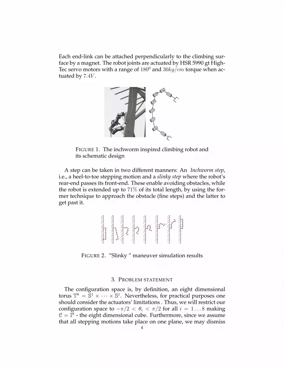
A step can be taken in two different manners: An Inchworm step,i.e., a heel-to-toe stepping motion and a slinky step where the robot’srear-end passes its front-end. These enable avoiding obstacles, whilethe robot is extended up to 71% of its total length, by using the for-mer technique to approach the obstacle (fine steps) and the latter toget past it.

FIGURE 2. ”Slinky ” maneuver simulation results

3. PROBLEM STATEMENT

The configuration space is, by definition, an eight dimensionaltorus T8 = S1 × · · · × S1. Nevertheless, for practical purposes oneshould consider the actuators’ limitations . Thus, we will restrict ourconfiguration space to −π/2 < θi < π/2 for all i = 1 . . . 8 makingC = I8 - the eight dimensional cube. Furthermore, since we assumethat all stepping motions take place on one plane, we may dismiss

4

FIGURE 3. ”Heel to toe” maneuver Simulation results

the first and last joints thus reducing the configuration space to thesix-dimensional cube I6. We denote the i-th joint position by:

(xi,yi) = (i∑

k=1

Lk cosk∑

m=1

θm,i∑

k=1

Lk sink∑

m=1

θm)

Where Lk is the length of the k-th link and θk is the angle betweenlinks k and k − 1.Summing up, we regard the configuration space as a torus T6 withan obstacle Oθ so that C = I6, where Oθ is defined exactly by the an-gles limitation equations defined above.

Obviously, we need to avoid obstacles in the robot’s work space as well.Such obstacles are formulated as a set of half plane (in the workspace) obstacles denoted by OX and OY . Thus, a point obstacle (x0,y0)in the work space will be avoided by keeping a ”safe distance” froma Cartesian rectangle surrounding it:

(1) ‖xi − x0‖ > ε , ‖yi − y0‖ > ε , ∀i = 1, . . . , n+ 1

In order to avoid self-collisions, i.e., disallow configurations wherethe distance between any two joints is less than ε > 0, we define anew obstacle and denote it by Ocol defined as:

(2) ‖xi − xj‖ > ε , ‖yi − yj‖ > ε , ∀i 6= j

3.1. Remark. For a given configuration c ∈ C we denote the travelingdistance (in the work space) of a given joint i, due to a resolution-sized step in joint j by s(c)i,j . For each configuration we define themaximal step size as s := maxi,j,c{s(c)i,j}. Obviously to avoid colli-sions ε should be greater then s, for simplicity we choose the samevalue for self collisions and obstacles. For the climbing robot thishappens for the distal joint when the entire robot is aligned and thebase joint is actuated.

5

Note that under our angle limitations, equation (2) is reduced tothe set of all pairs i, j where ‖i− j‖ ≥ 4.

Torque limitation is to be considered as well. We denote such anobstacle by OT , which is defined by the configurations where themaximal torque exerted on one or more of the actuators exceeds agiven torque T0. The torque (resulting at the base joint 1) is given by:

(3) T = mg

n−1∑k=1

xk +mgxn

2

Where n is the number of degrees of freedom (n = 6 in our case)and m is the mass of a single link (here, all links are assumed to behomogeneous).

FIGURE 4. Collision between second-node andseventh-node.

3.2. Remark. As a benchmark for the shortest path possible, the fol-lowing approach was taken: The torque T was calculated for all n-dimensional grid points (θ1, θ2, . . . , θn) = Nn where N = {−π/2,−π/2+∆θ, · · · , π/2} and ∆θ is the grid resolution taken here as π/6. Fixingn = 6 the configuration space volume exceeds 5 · 106 voxels, and themaximal number of neighbouring configurations for each configu-ration is

∑6k=1(C

k6 ) = 728 (Cn

m = m!n!(m−n)! ). This approach forces one

to make do with low resolutions, which, in turn, may result in largetranslations in the work space. Therefore this approach is not appli-cable for congestive obstacle zones.Nevertheless, we conducted several tests considering only twelvearcs γi,j for each configuration i (connecting it to its adjacent con-figuration j) , and reducing actuation to one motor at a time. In

6

addition, we considered a maximum endurable torque such that ifγi,j > Tmax we set γi,j to infinity. We then implemented Dijkstra’salgorithm in order to extract the shortest path connecting a givenorigin and goal configurations. Calculating Cfree took over an houron a dual-core PENTIUM IV platform, which makes this naive ap-proach non-applicable for real-time calculations, but still, qualita-tively demonstrates reasonable paths to compare our results with.

4. CPRM MOTION PLANNING SCHEME

As indicated above we would like to combine both potential fieldalgorithms with sampling-based algorithms. Our algorithm differsfrom a Probabilistic Road Map algorithm (PRM) in the motion be-tween a pair of anchoring points which takes place on the boundaryof the obstacle subspace O. We define a varying potential field f on∂O as a Morse function and follow ~∇f . Such an approach makesit possible for two non-mutually visible points to be connected andthus decreases runtime. We define a potential field as a Morse func-tion in C restricted to ∂O. Still, a situation at which ~∇f = 0 on a’large’ subspace is not welcome, since in such a place one would bedisoriented. In order to accommodate such a property we use a re-stricted Morse function as our potential field:

4.1. Defintion. Given M a compact n-dimensional smooth manifold anda smooth map f : M → R, we call p ∈ M a critical point of f if∂f/∂xi = 0 for all local coordinates xi of M at p. A critical point is said tobe non-degenerate if the Hessian matrix H = [∂2f/∂xi∂xj]

ni,j=1 is non-

singular at p. A Morse function of M is a smooth function f with onlynon-degenerate critical points (compare with [16]).

4.2. Fact ([17]). Surprisingly, it turns out that almost every smooth func-tion f : M → R is Morse . Furthermore, if g : M → R is a smoothfunction, then there exists a Morse function f : M → R arbitrarily closeto g.

Since we differentially follow the ~∇f , it is essential that f be aMorse function in order to avoid situations in which critical pointsare non-isolated (degenerated critical points).

4.1. The Algorithm: As described above, our motion planning al-gorithm is a crawling motion planner, i.e., whenever a configurationspace obstacle is met, motion is continued by crawling on its bound-ary, while motion in the ambient space is a linear one (see Figure 5).Since all the obstacles are ”convex” in a certain way we discuss in

7

Proposition 4.4, this method is sufficient for most situations. Still,there may be situations in which we will need to traverse n or moreobstacles at once, situation which could cause our algorithm to fail.In order to tackle this problem, we use a probabilistic method andcontinue our crawling scheme by redefining f . The algorithm workswell due to Fact 4.2 (alternatively, f can be corrected if slightly per-turbed).

We divide the configuration space into two subspaces - the free spaceCfree and the obstacle space O = Ocol∪OT∪iOxi ∪jOyj∪Oθ. We definetwo configuration-points ps, pg ∈ Cfree as the origin and goal config-urations. Motion in Cfree is carried out by following the ~l = pg − psdirection. So:

4.3. Defintion. In the free configuration space, f is defined as the Eu-clidean distance in C from current configuration pc to pg. Note that, ~∇f issimply ~l = pg − pc in Cfree.

When a path intersects O, motion is continued on O’s boundaryfollowing the direction of ~∇Of using the following: (1) calculate ~∇O(see section 3); (2) calculate the null space K to all ~∇O; (3) project ~lon K and proceed motion at the projection direction. This is carriedout until ~l leaves O, that is, until ~l points out of O.

(a) (b) (c)

FIGURE 5. A schematic view of the algorithm (a)Crawling on the obstacle’s surface, (b) Crawling ontwo obstacles, (c) Crawling on an obstacle O which in-tersects with an angle limitation boundary Oθ.

Let us denote ~ni as the normal to the i − th obstacle calculatedin the intersection configuration (see Figure 5(a)) When reaching aconfiguration which satisfies more than one obstacle we may ignore

8

Oi for which~l·~ni > 0. In configurations where all Oi maintain~l·~ni < 0(see Figure 5(c)), motion takes place at the null-space of all ~ni.

Algorithm 1: Morse-Crawling PseudocodeData Inputs ps,pe, Oi, Oj , C = [−pi2 , π2 ]

n

Output A path from ps to pe avoiding Oi, Oj .set pc = psPerturb f if it satisfies Equations 6 or 9.While f > 0 do:

If pc /∈ ∂O1, pc /∈ ∂O2

move linearly towards pe reducing f .If pc ∈ ∂Oi but pc /∈ ∂Oj

Follow ~∇∂Oif .

If pc ∈ ∂Oj as wellMove in perpendicularly to ~∇Oj

f and ~∇Oif reducing f .

4.2. Completeness of Algorithm 1. In order for f to be an efficientpotential field one would like to have f as Morse, preferably with nocritical points on ∂O. We will now prove that this is the case:

4.4. Proposition. The critical points of almost all potential field functionsf (as defined above) are not on Ox, Oy, Ocol, OT nor on Oθ.

Proof. We shall prove that for any given vector ∇f = ~l, there are nonormal vectors to ∂O ⊂ C which are equal to it (up to sign). Forbrevity we denote the set {θ1, θ2, . . . , θn} by Θ, and the sum

∑kj=1 θj

by Θk. Recall that the configuration space is defined in the orthogo-nal space bounded by θi = [−π

2, π2], for all i = 1, 2, ..., n. An obstacle

Ox (and OT ) is implicitly defined by:

(4) hx(Θ) =n∑i=1

ai cos(Θi)− x0

By differentiating we get: ∂hx∂θi

= −∑n

k=1 ak sin(Θk). We compare~∇hx = ~l to find points on ∂Ox whose normal equals the path di-rection ~l. Solving 4 we get:

(5)Θm = 2π(km + 1)− sin−1( lm+1−lm

am),

2πkm + sin−1( lm+1−lmam

)

where ln+1 = 0 and |km| ≤⌊m+14

⌋. assigning 5 to 4 we get the relation

(6)n∑

m=1

√a2m − (lm+1 − lm)2 = x0

9

This completes the proof for Ox. Clearly almost all ~l will not satisfythis, and even if it do we can and shall perturb f to avoid the appear-ance of such critical points.For Oy which is defined as a sum of sines rather then cosines, theproof is identical. Ocol where the j1’th joint and the j2’th joint (as-sume j2 > j1) collision is defined by:

hx(Θ) =

j2∑i=j1

ai cos(Θi)(7)

hy(Θ) =

j2∑i=j1

ai sin(Θi)(8)

By differentiating, equating to ~l and assigning to 7 we get:

(9)j2∑

m=j1

√a2m − (lm+1 − lm)2 = 0

Again we can and shall perturb f to avoid equality. �

4.5. Remark. A basic result of Morse theory states that almost all func-tions are Morse. More precisely since O is an immersed submanifoldin C ∈ Rn and f : C×O→ R which is given by f(o, c) = ‖o− c‖2 thenfor almost all c ∈ C the function fc = f(·, c) : O→ R is a Morse func-tion on O (see Milnor [18], p. 36). So actually any collision functionin the work space which defines a smooth manifold in C (e.g. point-point, point-segment, segment-segment, plane-point, etc.) togetherwith a function defined as a distance between current configuration(on O) and the target configuration will most likely end up to beMorse.

Consider a configuration c ∈ C which satisfies multiple manifoldsi ∈ I such that ~ni ·~l > 0 for all i ∈ I (here ni is the normal to the i-thmanifold at c). In this case, motion is confined to the n− ‖I‖ ≥ 0 di-mensional subspace. When equality is satisfied, our algorithm failsdue to the local minima. Since we consider a total of more than 14obstacles (one torque obstacle, mv ≥ 2 vertical (in the work space)obstacles, mh ≥ 1 horizontal obstacles and 10 self collision obstacles)local minima happens quite often.As for non-regular obstacles (i.e those that exhibit undefined deriva-tives in some point subset Σ) we apply the same rational that is, set-ting two anchoring points to be not-connected if the path betweenthem crosses Σ.

10

4.3. Road Map. In order to overcome the local minima problem weapply the probabilistic road map scheme: we randomly addm pointsin Cfree in addition to the ps, pg and examine pairwise connectivity.The resulting connectivity graph is weighted by the number of stepsneeded to transverse node pairs. Note that two nodes may be findto be connected using CPRM while for PRM they will not. In otherwords, CPRM algorithm reduces the number of nodes needed forsolution. So, for cases where just few nodes are needed the choiceof the algorithm makes no real difference. Here, we used Dijkstra’salgorithm to calculate the roadmap’s shortest path. Nevertheless, incases where many nodes are needed we believe that a DFS algorithmor some other uninformed search algorithm would be more efficientin the sense of elapsed time.

4.6. Remark. Note that, though not implemented here, graph connec-tivity algorithms may accelerate calculations when selectively addingnew nodes that should be checked for pairwise connectivity.

Algorithm 2: Crawling Probabilistic Road MapData Inputs ps,pg , m, {Oi}k>1

1 , C = [−pi2 , π2 ]n

Output The shortest path from ps to pg avoiding all OiGenerate m random points pr ∈ CfreeWhile shortest path is not obtained, do:

for all pi, pj , i 6= j, do:check connectivity between pi and pj (using algorithm 1).If points are connected:

grade the connected arc as the mean of theweight function on the connecting line.

If line convergent to local minima :set pi and pj as not connected.

use dijkstra to calculate shortest path from the graph.If no path is found: increase m.

4.4. parallelizing CPRM. Naturally, one may accelerate the calcula-tion runtime by applying parallel computation using multicore CPU(modern computers commonly possesses 2 − 8 cores). E. Plaku, etal. [19] have shown that RoadMap motion planning algorithms mayhave efficient parallel versions, up to almost linear speedup.Further runtime improvement can be achieved using a GPGPU ap-proach for motion planing (see [20], [21]) One can apply the SIMD(Single Instruction Multiple Data) methodology over Algorithm 2.Recall that Algorithm 2 determines the connectivity between all pairs

11

of anchoring points and therefore is suitable for parallel computing(requires limited size of data).

5. AN EXAMPLE: AN INCHWORM INSPIRED CLIMBING ROBOT

5.1. Simulation Results. A MATLAB program for controlling therobot was written. Commands were sent to a 16 servo pololu con-troller. Our implementation for crawling on the hyper-surfaces wascarried out by small steps with constant length.We compared the CPRM algorithm with the naive PRM algorithm.The program was given start and goal configurations and obstaclefunctions: wall obstacle, a rectangle obstacle, torque limitation andself intersection limitation. We determined start and goal configura-tions as:

pg = (π/2, 0, . . . , 0, π/2)︸ ︷︷ ︸n

, ps = (−π/2, 0, . . . , 0,−π/2)︸ ︷︷ ︸n

for a sequence of dimensions n = 3, 4, 5..., 16.

FIGURE 6. A three anchoring point solution via CPRM

FIGURE 7. A seven anchoring point solution via CPRM

The naive algorithm selects k = 1 random anchoring points inCfree. Mutual connectivity for all pairs of points is calculated to forma graph, each arc is given weight corresponding to the energy con-sumption needed for the given move. The shortest path is then cal-culated using Dijkstra algorithm. If no path is found an additionalpoint is selected to form a weighted graph with k + 1 nodes. Notice

12

that using this method is highly time-consuming. Still, since our goalis to compare anchoring point and calculation time for a successiveexperiment, calculation time is reset to zero when k is increased. Thealgorithm proceeds in adding points until a solution is found (for sayk = kf points). Finally, we keep track of the elapsed time for the finalset kf of anchoring points.

Similarly we ran the CPRM algorithm using the same procedure,i.e. starting with k = 1 random points, adding points when neededup to kf . Again, we make record of time elapsed for the successful kfsee Figure 8. Note that this is a stringent measure since the total dif-ference in the elapsed time between both motion planning schemesis bigger than that depicted (may be proved inductively). Due to theadditional crawling feature the number of anchoring points neededfor obtaining a path from start to goal is presumed to be smaller.Figure 8 depicts an average of 10 experiments for each dimension.Indeed, any PRM algorithm results in an exponential number of an-choring points. The CPRM demands an average of less then 10% ofthe PRM anchoring points.

FIGURE 8. Number of anchoring points

Figure 9 compares between CPRM and PRM elapsed time. Need-less to say, reducing the number of nodes is essential for real-timesystems, and as seen here CPRM presents a major advantage.

Although one may suspect that the PRM algorithm establishes apseudo-linear (PL) approximation of the CPRM algorithm, the lengthof the path in each algorithm is different, as can be seen in Figure 10.This also points at the efficiency of the CPRM.

6. ADDITIONAL EXPERIMENTS

In order to get a clear estimate of our algorithm performances wehave conducted two additional experiments using the well known

13

FIGURE 9. Elapsed time

FIGURE 10. path length

cage setup and the puma-bars setup:

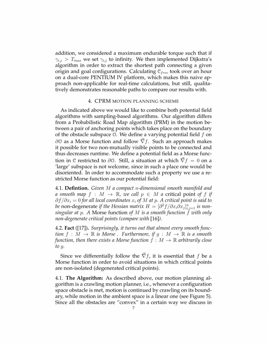
The cage setup: depicted in Figure 11 where an ’L’ shape is con-fined in an octagon prism bird’s cage. The task is to exit the cage.This setup was experimented by Yershova and Lavelle [22] (a tighterversion known as the Hedgehog problem was solved but not for-mally published by V. Vonasek.) Yershova and Lavelle [23] reporteda set of 37, 634 nodes required for solution and a computation timeof 191 seconds for the MPNN algorithm; a 37, 186 nodes and 2, 302seconds for a naive PRM; a 35, 814 nodes and 187 seconds for Covertree algorithm, and 37, 922 anchoring points with a 361 seconds cal-culation time applying sb(s). The shortest calculation time given in[22] is reported as 21 seconds.

We have performed a set of 100 tests using CPRM . Initial and targetconfiguration were randomly selected (in and out of the cage). The’L’ shape taken as unit length for both its horizontal and vertical seg-ments, with a 0.3 × 0.3 rectangle profile, the bars where taken as 0.1diameter and 2.2 for the overall (middle) diameter of the cage. Colli-sions were calculated as intersections between line-segments (rather

14

MPNN PRM cover tree sb(s) CPRMcomputation time [sec] 191 2,302 187 361 7.8number of nodes 37,634 37,186 35,814 37,922 3

TABLE 1. Simulation results of some motion plannersfor the cage setup.

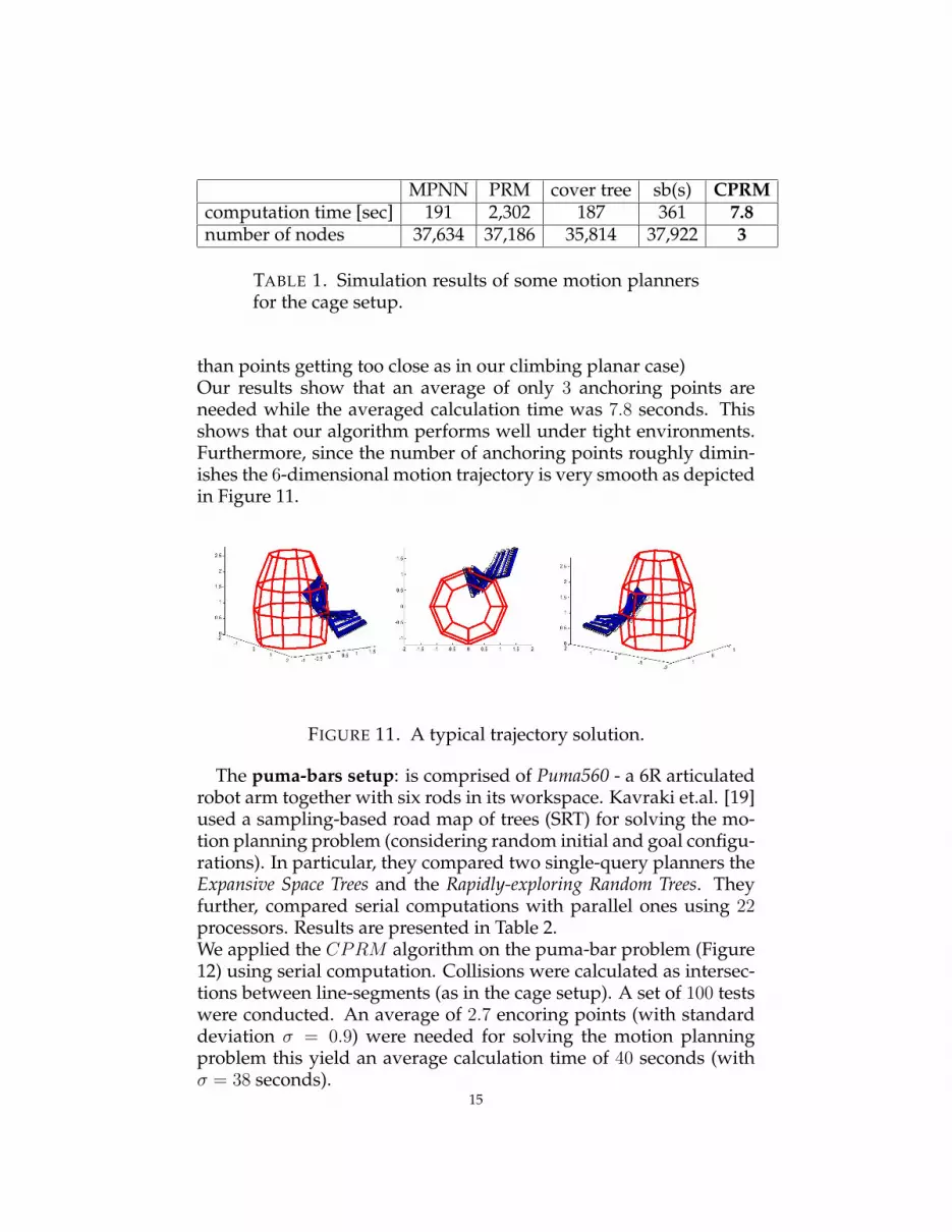
than points getting too close as in our climbing planar case)Our results show that an average of only 3 anchoring points areneeded while the averaged calculation time was 7.8 seconds. Thisshows that our algorithm performs well under tight environments.Furthermore, since the number of anchoring points roughly dimin-ishes the 6-dimensional motion trajectory is very smooth as depictedin Figure 11.

FIGURE 11. A typical trajectory solution.

The puma-bars setup: is comprised of Puma560 - a 6R articulatedrobot arm together with six rods in its workspace. Kavraki et.al. [19]used a sampling-based road map of trees (SRT) for solving the mo-tion planning problem (considering random initial and goal configu-rations). In particular, they compared two single-query planners theExpansive Space Trees and the Rapidly-exploring Random Trees. Theyfurther, compared serial computations with parallel ones using 22processors. Results are presented in Table 2.We applied the CPRM algorithm on the puma-bar problem (Figure12) using serial computation. Collisions were calculated as intersec-tions between line-segments (as in the cage setup). A set of 100 testswere conducted. An average of 2.7 encoring points (with standarddeviation σ = 0.9) were needed for solving the motion planningproblem this yield an average calculation time of 40 seconds (withσ = 38 seconds).

15

Serial Serial Parallel Parallel CPRMSRT[RRT] SRT[EST] SRT[RRT] SRT[EST]

computation time [sec] 8,097 10,207 327 414 40

TABLE 2. Simulation results of some motion plannersfor the puma bars setup.

FIGURE 12. The Puma bar setup. Vertical bars diame-ter was set to 4 [inch], while the robot’s forearm lengthis 17.05 [inch].

7. CONCLUSIONS

Motion planning via the configuration space is necessary for hyper-redundant robots requiring challenging maneuvers. Our results im-ply that combining the naive PRM algorithm with the potential fieldmethod significantly shortens calculation time. The CPRM algo-rithm is applicable for mechanisms whose configuration spaces arealgebraically known, yet one may apply CPRM also for experimen-tally derived configuration spaces whose algebraic form is not known,and is too complex for real-time calculations. This may be done viaconfiguration space compression and region-of-interest decompres-sion. We plan to investigate such a generalized approach in the fu-ture.

16

FIGURE 13. The algorithm applied on 10 DOF climb-ing robot

8. ACKNOWLEDGEMENTS

We would like to acknowledge the anonymous reviewers for theirfruitful comments.

REFERENCES

[1] Z. Jianwen, S. Lining, D. Zhijiang, and Z. Bo, “Self-motion analysis on a re-dundant robot with a parallel/series hybrid configuration,” in Control, Au-tomation, Robotics and Vision, 2006. ICARCV ’06. 9th International Conference on,dec. 2006, pp. 1 –6.

[2] H. Brown, M. Schwerin, E. Shammas, and H. Choset, “Design and control ofa second-generation hyper-redundant mechanism,” in Intelligent Robots andSystems, 2007. IROS 2007. IEEE/RSJ International Conference on, 29 2007-nov. 22007, pp. 2603 –2608.

[3] S. Kornienko, O. Kornienko, A. Nagarathinam, and P. Levi, “From real robotswarm to evolutionary multi-robot organism,” in Evolutionary Computation,2007. CEC 2007. IEEE Congress on. IEEE, 2007, pp. 1483–1490.

[4] H. Maruyama and K. Ito, “Semi-autonomous snake-like robot for search andrescue,” in Safety Security and Rescue Robotics (SSRR), 2010 IEEE InternationalWorkshop on, july 2010, pp. 1 –6.

[5] T. Ota, A. Degani, D. Schwartzman, B. Zubiate, J. McGarvey, H. Choset, andM. Zenati, “A highly articulated robotic surgical system for minimally inva-sive surgery,” The Annals of Thoracic Surgery, vol. 87, pp. 1253–1256, May 2009.

[6] H.-S. Yoon and B.-J. Yi, “A 4-dof flexible continuum robot using a spring back-bone,” in Mechatronics and Automation, 2009. ICMA 2009. International Confer-ence on, aug. 2009, pp. 1249 –1254.

[7] K. Xu and N. Simaan, “Actuation compensation for flexible surgical snake-like robots with redundant remote actuation,” in Robotics and Automation,2006. ICRA 2006. Proceedings 2006 IEEE International Conference on, may 2006,pp. 4148 –4154.

[8] M. Akhtaruzzaman and A. Shafie, “Evolution of humanoid robot and con-tribution of various countries in advancing the research and development ofthe platform,” in Control Automation and Systems (ICCAS), 2010 InternationalConference on, oct. 2010, pp. 1021 –1028.

[9] B. Siciliano and O. Khatib, Springer handbook of robotics. Springer-Verlag NewYork Inc, 2008.

[10] J. Kuffner, K. Nishiwaki, S. Kagami, M. Inaba, and H. Inoue, “Motion plan-ning for humanoid robots,” Robotics Research, pp. 365–374, 2005.

[11] D. Yagnik, J. Ren, and R. Liscano, “Motion planning for multi-link robotsusing artificial potential fields and modified simulated annealing,” in Mecha-tronics and Embedded Systems and Applications (MESA), 2010 IEEE/ASME Inter-national Conference on, july 2010, pp. 421 –427.

[12] A. Masoud, “A discrete harmonic potential field for optimum point-to-pointrouting on a weighted graph,” in Intelligent Robots and Systems, 2006 IEEE/RSJInternational Conference on, oct. 2006, pp. 1779 –1784.

[13] S. Khanmohammadi and A. Mahdizadeh, “Density avoided sampling: Anintelligent sampling technique for rapidly-exploring random trees,” in HybridIntelligent Systems, 2008. HIS ’08. Eighth International Conference on, sept. 2008,pp. 672 –677.

[14] L. Kavraki, J. Latombe, R. Motwani, and P. Raghavan, “Randomized queryprocessing in robot path planning,” in Proceedings of the twenty-seventh annualACM symposium on Theory of computing. ACM, 1995, pp. 353–362.

[15] B. M. B. Medina O, Taitz A. and S. N., “Configuration space Compression Forkinematically redundant robots,” PrePrint.

[16] E. Rimon and D. Koditschek, “Exact robot navigation using artificial potentialfunctions,” IEEE Transactions on robotics and automation, vol. 8, no. 5, pp. 501–518, 1992.

[17] X. Ni, M. Garland, and J. Hart, “Fair morse functions for extracting the topo-logical structure of a surface mesh,” in ACM Transactions on Graphics (TOG),vol. 23, no. 3. ACM, 2004, pp. 613–622.

[18] J. Milnor, Morse theory. Princeton Univ Pr, 1963.

18

[19] E. Plaku, K. Bekris, B. Chen, A. Ladd, and L. Kavraki, “Sampling-basedroadmap of trees for parallel motion planning,” Robotics, IEEE Transactionson, vol. 21, no. 4, pp. 597–608, 2005.

[20] A. Bleiweiss, “Gpu accelerated pathfinding,” in Proceedings of the 23rd ACMSIGGRAPH/EUROGRAPHICS symposium on Graphics hardware. Eurograph-ics Association, 2008, pp. 65–74.

[21] J. Kider, M. Henderson, M. Likhachev, and A. Safonova, “High-dimensionalplanning on the gpu,” in Robotics and Automation (ICRA), 2010 IEEE Interna-tional Conference on. IEEE, 2010, pp. 2515–2522.

[22] A. Atramentov and S. LaValle, “Efficient nearest neighbor searching for mo-tion planning,” in Robotics and Automation, 2002. Proceedings. ICRA’02. IEEEInternational Conference on, vol. 1. IEEE, 2002, pp. 632–637.

[23] A. Yershova and S. LaValle, “Improving motion-planning algorithms by effi-cient nearest-neighbor searching,” Robotics, IEEE Transactions on, vol. 23, no. 1,pp. 151–157, 2007.

19