A preliminary investigation of welfare migration induced by time limits (Mark L. Burkey)

A Preliminary Investigation of Welfare Migration Induced by Time Limits Hal W. Snarr and Mark L. Burkey North Carolina A&T State University - USA

Abstract. Studies on welfare programs in the United States have identified three types of welfare

migration (employment, benefit, and amenity-related). This paper introduces a fourth type of migration induced by welfare time limits. After a welfare-dependent family runs out of benefits, it is possible for them to reset the Temporary Assistance for Needy Families time clock by crossing state lines to extend their benefits. Our theoretical results suggest that the likelihood of migration increases if the migration distance is small or the gain from the move is large. We hypothesize that, ceteris paribus, families migrating in order to extend their bene-fits will minimize the distance they migrate, and will be likely to move into the nearest state, especially into counties just across the state border. We utilize macro data at the county level to look for evidence of time-limit induced migration. Estimates indicate that time limits may be associated with an increase in welfare migration.

1. Introduction In 1996 the U.S. Congress passed the Personal Re-sponsibility and Work Opportunity Reconciliation Act of 1996 (PRWORA). PRWORA altered the rules gov-erning federal funding of welfare and disbursement of aid to qualifying households by replacing Aid to Fami-lies with Dependent Children (AFDC) with Tempo-rary Assistance for Needy Families (TANF). Specifi-cally, TANF allowed the States to tailor their welfare programs as they saw fit, and altered how the Federal government provided funding to the states. However, states were encouraged to impose lifetime limits1, in-crease work requirements and strengthen sanctions. A majority of TANF studies done recently present evi-dence suggesting that the welfare reforms adopted by PRWORA have numerous unintended consequences that negatively impact the well-being of the nation’s poor (Brueckner, 2000; Kaestner, Kaushal and Van Ryzin, 2003; Grogger and Michalopoulos, 2003; Grog-ger, 2003, 2004a and 2004b, and De Jong, Graefe, and

1 If states allow welfare recipients to stay on welfare for more than 5 years, the state bears the full cost of these benefits. Michigan and Vermont have not imposed any time limits (See Table 5).

St. Pierre, 2005). Brueckner (2000) summarizes the theoretical and empirical evidence supporting the existence of a “race to the bottom” in benefits that has resulted due to the shift from matching grants under the old AFDC rules to the block grants used in the TANF program. Ac-cording to Brueckner, the race to the bottom in bene-fits arises from the belief among state policy makers that benefit-related immigration will occur if their state is more generous than a neighboring state. Though the empirical evidence verifying the existence of benefit-related migration is inconclusive, the policy makers’ fear of becoming a “welfare magnet” results in the equalizing of benefits at socially undesirable levels (Southwick, 1981; Gramlich and Laren, 1984; Blank, 1988; Walker, 1994; Levine and Zimmerman, 1995; Enchautegui, 1997; Borjas, 1998; and Meyer, 1998). Kaestner et al. (2003) propose that a race to the bottom in benefits is not the only unintended conse-quence of the TANF provisions. They argue that TANF time limits reduce the present value of benefit differentials between states, which in turn lowers benefit-related migration. They also claim that work requirements and stiffer sanctions increase the likeli-

Special Section on Migration - JRAP 36(2): 124-139. © 2006 MCRSA. All Rights Reserved.

Welfare Migration & Time Limits 125

hood of employment-related migration among low-income single mothers. The estimates of De Jong et al. (2005) imply that welfare reform has stimulated inter-state immigration. These results seem plausible since TANF participation requires welfare recipients to work or participate in a training program in many states. If an area’s neighbors have more robust economies, welfare recipients living in the depressed economy may migrate for employment reasons. The estimates of Kaestner et al. (2003) suggest that TANF welfare policies have reduced all forms of migration other than employment-related migration. The welfare reform literature, comprehensively reviewed in Grogger, Karoly and Klerman (2002), and the emerging time-limited welfare literature (e.g., Kaushal and Kaestner, 2001; Grogger and Michalopou-los, 2003; and Grogger, 2003, 2004a and 2004b) exam-ine the impacts of reforms such as work requirements, time limits and sanctions on caseloads and participa-tion. These studies have all come to a similar conclu-sion: reforms such as time limits generally reduce par-ticipation and state caseloads. Much of the welfare reform literature attempts to determine which factors are associated with the large fall in the caseload. For example, Fang and Keane (2004) attribute 57, 26, 11, and 7 percent of the caseload reduction between 1993 and 2000 to work requirements, the Earned Income Tax Credit, time limits, and the economy of the late 1990s, respectively. The literature on time limits delves a little deeper by looking at child outcomes. According to Grogger and Michalopoulos (2003) and Grogger (2003, 2004a, 2004b), time limits unintentionally reduce welfare par-ticipation the most among families that need assis-tance the most—those with young children. On the other hand, Kaushal and Kaestner (2001) find that the imposition of time limits has had a positive impact on low-educated, unmarried women with children. They found that women who left welfare for employment work nearly 30 hours per week on average, represent-ing a large improvement in their financial status even at low-skilled wages. Most of the welfare migration literature has fo-cused on interstate benefit-related migration, which investigates the propensity for families to move to a state with higher benefit levels. Kaestner et al. (2003) study employment-related and amenity-related migra-tion, where families may have an incentive to move in order to take advantage of better job markets or other desirable characteristics of a region. We introduce a fourth type of migration induced explicitly by welfare time limits—for the remainder of this paper we refer to this type of migration as time-limit migration. As previously mentioned, Kaestner et al. (2003)

reason that because TANF lowers the present value of lifetime benefits, migration is likely to decrease. This prediction neglects the fact that when benefits run out in one state, it is possible to move to a different state to re-enroll. This also assumes that welfare recipients have long planning horizons and low discount rates, which is assumed by studies such as Grogger and Michalopoulos (2003) and Swann (2005). In contrast, Snarr and Axelsen (2006) argue that they are likely to have high discount rates as evidenced by their bor-rowing behavior. As discussed in Stegman and Faris (2003), families with a history of being on welfare are highly likely to borrow at high interest rates from payday lenders, even though these institutions appear to avoid neighborhoods with high rates of welfare par-ticipation2 (Burkey and Simkins, 2004). Therefore, changes in income streams far in the future are unlikely to impact the current decision making in this population. If welfare households desire to stay on welfare, they may decide to migrate to extend their benefits. And, according to Meyer (1998), the likeli-hood of this form of migration increases the closer the household lives to the nearest state border because the cost of such a move is relatively small with respect to its short-term gain in household income.3

Consider the decision of a welfare-dependent fam-ily in Los Angeles, California whose benefits have run out. Such a family would have to move quite a dis-tance to reach a neighboring state and sign up for new benefits, and will likely seek employment. Contrast this with the decision of residents in adjacent counties A and B, separated only by a state borderline. When welfare recipients in these two counties begin to run out of benefits, families from county A may move to county B and sign up for benefits again, and vice versa. In these counties welfare enrollment rates will not drop, as the counties will merely be exchanging beneficiaries. We refer to the possibility that recipients living along state-lines might “jump” across the bor-der in order to extend their welfare benefits as the “welfare-flipping hypothesis”. Several factors make welfare flipping possible: First, according to the U.S. Department of Health and Human Services (2000a), even though PRWORA re-quires the States to enforce federally-mandated time limits and exchange information, states do not cur-

2 Instead, they prefer the working poor as customers. 3 Migration between Portland, OR and Vancouver, WA, is an exam-ple of how inexpensive time-limit migration can be. Portland and Vancouver are separated only by the Columbia River, which hap-pens to be the southern border between these states. Two interstate bridges, I-205 and I-5, connect the two communities. To counter this, states like Washington, Idaho and Oregon are in the process of forming data-sharing agreements to detect abuses.

126 Snarr and Burkey

rently share data. Second, according to Lindert (2005), the failure to set up a national database has hindered the enforcement of time limits and has allowed some individuals to “double dip” by simultaneously collect-ing benefits in two states at once. Lastly, although several states have tried to limit benefits in various ways for immigrants, the U.S. Supreme Court has struck down these attempts citing the Privileges and Immunities Clause of the Fourteenth Amendment.4

This paper essentially merges the welfare reform and welfare migration literatures. We do this by rec-ognizing that if households understand that assistance ends in x months, households must eventually work when their benefits expire. For many reasons, house-holds participating in welfare may want to extend their benefits by welfare-flipping. Perhaps these households are unable, unwilling, or ill-prepared to leave the welfare rolls so they choose to migrate to a nearby state if the cost associated with the move is relatively small. After TANF benefits run out, a household will receive no assistance if it remains in its home state. However, if this household considers mi-grating to the nearest state, the benefit differential is actually quite large—much larger than benefit differ-entials considered previously in the literature. Since the states do not share data and minimum residency requirements are not imposed, the benefit differential is equal to a neighboring state’s benefit payment. Be-cause there are costs associated with migration, time-limit migration will be more likely along state borders. If a race to the bottom in benefits has occurred, then state benefit levels have already reached an “insuffi-ciently generous” equilibrium (Brueckner, 2000). This raises the question: If benefit levels have reached equi-librium and low-income households are still migrat-ing, what incentive are they responding to? The mi-gration literature, surveyed extensively by Meyer (1998) and Brueckner (2000), and the time-limited wel-fare literature (Kaushal and Kaestner, 2001; Grogger and Michalopoulos, 2003; and Grogger, 2003, 2004a and 2004b) have not yet studied the possibility that migration can be induced by time limits. 2. Welfare Migration Theory To demonstrate the effect of time limits on the mi- 4 Prior to 1969 states could impose minimum residency require-ments on U.S. citizens that had just recently emigrated from other states (U.S. Department of Health, Education, and Welfare, 1969). By the end of 1969, according to Rosenheim (1970), the U.S. Supreme Court ruled that minimum residency requirements were unconstitu-tional. More recently, the U.S. Supreme Court ruled that Califor-nia’s practice of paying immigrants the benefit they would have received from the state they moved from was unconstitutional (Saenz v. Roe, 526 U.S. 489, 1999).

gration of welfare families we analyze a simple two-period utility model. Our model differs from those found in the migration literature (Brown and Oates, 1987; Wildasin, 1991; Brueckner, 2000; and Kaestner et al., 2003) because we model the effect time limits have on the decision to migrate in the final month of TANF eligibility. With this in mind, period one represents the final month of eligibility for a household living in its home state. In period two the household can par-ticipate in welfare if it migrates to the nearest state. However, if it does not migrate it cannot use welfare because it runs out of eligibility. We assume that households considering migration maximize the fol-lowing two-period utility function:

1 2 1 2( , ) ln( ) ln( )u c c c cβ= + (1) where ct denotes the household’s consumption in pe-riod t, and β is the household’s discount factor, which is assumed to be positive and less than one. We let m denote the migration decision: m = 1 if the household migrates, 0 otherwise. Following Brueckner (2000), we assume state out-put depends on the size of the low-skilled labor force (N) given fixed levels of capital and land, and so that the wage rate is determined by ( )w f N′= (2) where ( )f N′ is the marginal product of the Nth worker. Assuming diminishing marginal productivity, immigration lowers the low-skilled wage rate. If the household participates in welfare, its income includes the cash grant G from the government (benefit level) and wh labor market earnings, where h is the number of hours the household works on welfare (h ≥ 0). Households that do not participate in welfare earn wH dollars per period, where H represents full participa-tion in the labor market (h ≤ H). If the household mi-grates, it incurs a cost of ( d Fκ + ) dollars where κ is the per unit migration cost of moving distance d units and F is the fixed cost of the move. As a basis for comparison, we first consider the migration decision of a household under a lifetime entitlement policy. Such households maximize equa-tion (1) subject to

1 2( ) ( )(1 )n nG wh G w h d F m G wh m c cκ β β + + + − − + + − = + (3a)

where the superscript n identifies the neighboring state’s cash grant and wage rate. The solution to this problem uses a two-step procedure: First, the house-


hold determines its optimal level of consumption in both periods, conditional on the migration decision. Optimal consumption in both periods is given by cE in this Entitlement regime:

( ) ( )( )1

n nE G wh G G w h wh d F m G whc m κ β β

β+ + − + − − − + +

=+

(4.a)

Given this function, the household decides to mi-grate or not. If migration makes the household better off, it migrates. Substituting equation (4) into equation (1) yields the household’s indirect utility function un-der the lifetime entitlement policy: ( ) ( )ln ( ) ln ( )E E E

mv c m c mβ= +

The household migrates if its indirect lifetime util-ity from migrating ( 1

Ev ) exceeds its indirect lifetime

utility of staying ( 0Ev ). The following proposition de-

scribes the household’s optimal migration decision under a lifetime entitlement policy:5 PROPOSITION 1. Migration occurs if d is less than the critical distance

( ) ( )n nE G G w h wh Fd

κ− + − −

= (5.a)

The larger the critical distance, the more migration will occur because more welfare-eligible households will live within dE of the nearest county across the state border. Note that this condition is composed of two “differentials” between the home and a neighbor-ing state, one comparing benefit levels and one com-paring wage levels. Proposition 1 is consistent with the results found in Brueckner (2000) and Kaestner et al. (2003). Given the home state’s cash grant (G) and earnings (wh), neighboring states with higher benefits (G n) or wage rates (wn) have larger differentials. Lar-ger differentials raise the critical distance, and thus increase the probability of migration. Because states with high benefit levels (magnet states) attract immi-grants, their labor force (N) grows, causing the wage rate in magnet states to fall. This implies that wages in magnet states are driven down by benefit-related mi-gration. Thus, benefit-related migration will some-what offset the incentive for employment-related mi-gration, which may explain why the results in the mi-gration literature is mixed. Under time limits, the household’s two-period budget constraint is given by

5 All proofs are in the Appendix.

1 2( ) (1 )n nG wh G w h d F m wH m c cκ β β + + + − − + − = + (3.b)

Optimal consumption in both periods is given by cT in this Time limit regime:

( )( )1

n nT G wh G w h wH d F m wHc m κ β β

β+ + + − − − +

=+

(4.b)

The following proposition describes the household’s optimal migration decision under the time limit pol-icy: PROPOSITION 2. Time-limit migration occurs if the distance to the nearest state is less than the critical distance d T ( 0) ( )n n

T G w h wH Fdκ

− + − −= . (5.b)

Comparing Propositions 1 and 2 yields some in-teresting conclusions concerning time limits. First, the benefit differential is larger under time limits. As dis-cussed earlier, the benefit differential under time lim-its is the amount of the cash grant offered in the near-est state (G n), which is much larger than it would be had the state not imposed a time limit (G n – G). Con-versely, the earnings differential (wnh − wH) is smaller in states that have imposed time limits than it is for states that have not (wnh − wh) since H was assumed to be larger than h. The earnings differential is also af-fected by the size of the low-skilled labor force. Thus, households that are in their last month of eligibility are faced with a larger benefit differential but a smaller earnings differential than would have existed if their home state had not imposed time limits. This suggests that time limits have two opposing effects on migration, which raises the question: Which effect is larger? Time limits induce welfare migration if the critical distance increases after time limits are imposed, ceteris paribus:6 0T E G wh wHd d

κ+ −

− = > (6)

This inequality holds only if income available on welfare in the household’s home state ( )G wh+ is larger than it would have been off welfare (wH). Thus, emigration from time-limit states is influenced by the benefit levels they choose. If these states are located

6 If one includes the disutility of work in the model, then the earn-ings differential become a less powerful influence on the migration decision.


near entitlement states, the latter are likely to become even stronger welfare magnets under TANF than un-der the old AFDC rules. This is true for two reasons: First, entitlement states experience very little emigra-tion because they did not impose time limits. Second, entitlement states may receive considerable immigra-tion from nearby time-limit states. Furthermore, in regions where states are smaller such as in the North-east, more welfare flipping is likely to occur as most state residents will live near the border of at least one other state. 3. Data The data for the analysis come from the 1990 and 2000 U.S. Censuses and the Regional Economic Infor-mation System (REIS). The variable definitions and sources for the study are listed in Table 1. The U.S. Census datasets allow us to compare welfare enroll-ment rates between border and nonborder counties that are likely to be affected by time limits (Meyer, 1998 and McKinnish, 2005). These censuses are oppor-tune because many households that were on welfare when PRWORA was enacted in 1996 would be reach-

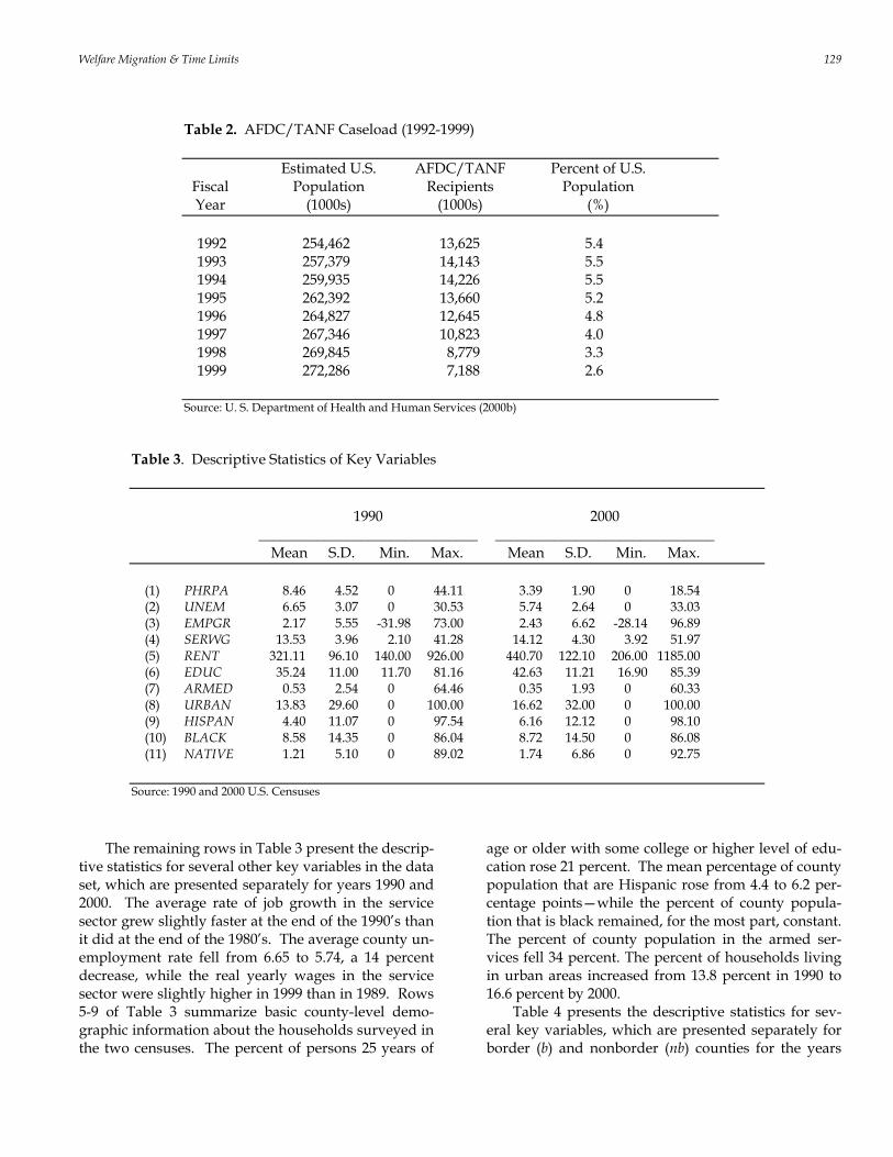
ing their respective time limits by the year 2000. The 1990 and 2000 census data gives us a clear before and after picture of welfare utilization rates of our target and control groups. The actual welfare caseload and its percent of population changed between 1992 and 1999 is shown in Table 2. According to Table 2, the caseload and the percent of households on welfare peaked in 1994. The decline in the welfare caseload from its peak is the largest in U.S. history, and the percentage of the popu-lation on welfare in 1999 of 2.6 percentage points was the lowest it had been since 1965 (U.S. Department of Health and Human Services, 2000b). From 1992 to 1999 the participation rate fell 52 percent. In our data analysis we define the welfare enrollment rate as the percentage of households that reported receiving pub-lic assistance. In the first row of Table 3 one sees a similar decrease in welfare enrollment using this defi-nition. Computed from the 1990 and 2000 U.S. Cen-suses, our variable suggests that county participation rates fell by nearly 60 percent over a slightly longer period of time.

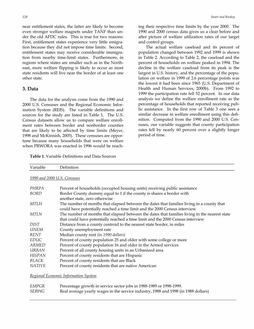
Table 1. Variable Definitions and Data Sources Variable Definition 1990 and 2000 U.S. Censuses PHRPA Percent of households (occupied housing units) receiving public assistance BORD Border County dummy equal to 1 if the county is shares a border with another state, zero otherwise MTLH The number of months that elapsed between the dates that families living in a county that

could have potentially reached a time limit and the 2000 Census interview MTLN The number of months that elapsed between the dates that families living in the nearest state

that could have potentially reached a time limit and the 2000 Census interview DIST Distance from a county centroid to the nearest state border, in miles UNEM County unemployment rate RENT Median county rent (in 1990 dollars) EDUC Percent of county population 25 and older with some college or more ARMED Percent of county population 16 and older in the Armed services URBAN Percent of all county housing units in an Urbanized area HISPAN Percent of county residents that are Hispanic BLACK Percent of county residents that are Black NATIVE Percent of county residents that are native American Regional Economic Information System

EMPGR Percentage growth in service sector jobs in 1988-1989 or 1998-1999. SERWG Real average yearly wages in the service industry, 1988 and 1998 (in 1988 dollars)


Table 2. AFDC/TANF Caseload (1992-1999) Estimated U.S. AFDC/TANF Percent of U.S. Fiscal Population Recipients Population Year (1000s) (1000s) (%) 1992 254,462 13,625 5.4 1993 257,379 14,143 5.5 1994 259,935 14,226 5.5 1995 262,392 13,660 5.2 1996 264,827 12,645 4.8 1997 267,346 10,823 4.0 1998 269,845 8,779 3.3 1999 272,286 7,188 2.6 Source: U. S. Department of Health and Human Services (2000b)

Table 3. Descriptive Statistics of Key Variables 1990 2000 ______________________________ ______________________________ Mean S.D. Min. Max. Mean S.D. Min. Max. (1) PHRPA 8.46 4.52 0 44.11 3.39 1.90 0 18.54 (2) UNEM 6.65 3.07 0 30.53 5.74 2.64 0 33.03 (3) EMPGR 2.17 5.55 -31.98 73.00 2.43 6.62 -28.14 96.89 (4) SERWG 13.53 3.96 2.10 41.28 14.12 4.30 3.92 51.97 (5) RENT 321.11 96.10 140.00 926.00 440.70 122.10 206.00 1185.00 (6) EDUC 35.24 11.00 11.70 81.16 42.63 11.21 16.90 85.39 (7) ARMED 0.53 2.54 0 64.46 0.35 1.93 0 60.33 (8) URBAN 13.83 29.60 0 100.00 16.62 32.00 0 100.00 (9) HISPAN 4.40 11.07 0 97.54 6.16 12.12 0 98.10 (10) BLACK 8.58 14.35 0 86.04 8.72 14.50 0 86.08 (11) NATIVE 1.21 5.10 0 89.02 1.74 6.86 0 92.75 Source: 1990 and 2000 U.S. Censuses

The remaining rows in Table 3 present the descrip-tive statistics for several other key variables in the data set, which are presented separately for years 1990 and 2000. The average rate of job growth in the service sector grew slightly faster at the end of the 1990’s than it did at the end of the 1980’s. The average county un-employment rate fell from 6.65 to 5.74, a 14 percent decrease, while the real yearly wages in the service sector were slightly higher in 1999 than in 1989. Rows 5-9 of Table 3 summarize basic county-level demo-graphic information about the households surveyed in the two censuses. The percent of persons 25 years of

age or older with some college or higher level of edu-cation rose 21 percent. The mean percentage of county population that are Hispanic rose from 4.4 to 6.2 per-centage points—while the percent of county popula-tion that is black remained, for the most part, constant. The percent of county population in the armed ser-vices fell 34 percent. The percent of households living in urban areas increased from 13.8 percent in 1990 to 16.6 percent by 2000. Table 4 presents the descriptive statistics for sev-eral key variables, which are presented separately for border (b) and nonborder (nb) counties for the years


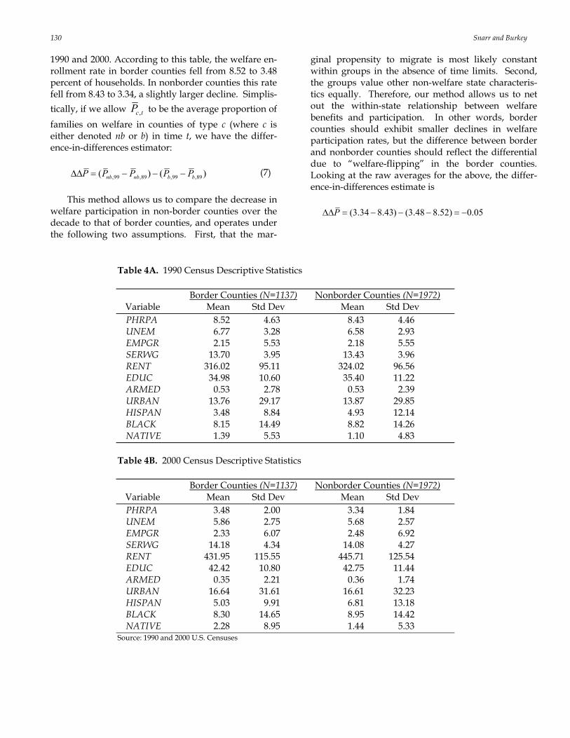
1990 and 2000. According to this table, the welfare en-rollment rate in border counties fell from 8.52 to 3.48 percent of households. In nonborder counties this rate fell from 8.43 to 3.34, a slightly larger decline. Simplis-tically, if we allow ,c tP to be the average proportion of families on welfare in counties of type c (where c is either denoted nb or b) in time t, we have the differ-ence-in-differences estimator: ,99 ,89 ,99 ,89( ) ( )nb nb b bP P P P P∆∆ = − − − (7) This method allows us to compare the decrease in welfare participation in non-border counties over the decade to that of border counties, and operates under the following two assumptions. First, that the mar-

ginal propensity to migrate is most likely constant within groups in the absence of time limits. Second, the groups value other non-welfare state characteris-tics equally. Therefore, our method allows us to net out the within-state relationship between welfare benefits and participation. In other words, border counties should exhibit smaller declines in welfare participation rates, but the difference between border and nonborder counties should reflect the differential due to “welfare-flipping” in the border counties. Looking at the raw averages for the above, the differ-ence-in-differences estimate is (3.34 8.43) (3.48 8.52) 0.05P∆∆ = − − − = −

Table 4A. 1990 Census Descriptive Statistics Border Counties (N=1137) Nonborder Counties (N=1972) Variable Mean Std Dev Mean Std Dev PHRPA 8.52 4.63 8.43 4.46 UNEM 6.77 3.28 6.58 2.93 EMPGR 2.15 5.53 2.18 5.55 SERWG 13.70 3.95 13.43 3.96 RENT 316.02 95.11 324.02 96.56 EDUC 34.98 10.60 35.40 11.22 ARMED 0.53 2.78 0.53 2.39 URBAN 13.76 29.17 13.87 29.85 HISPAN 3.48 8.84 4.93 12.14 BLACK 8.15 14.49 8.82 14.26 NATIVE 1.39 5.53 1.10 4.83 Table 4B. 2000 Census Descriptive Statistics Border Counties (N=1137) Nonborder Counties (N=1972) Variable Mean Std Dev Mean Std Dev PHRPA 3.48 2.00 3.34 1.84 UNEM 5.86 2.75 5.68 2.57 EMPGR 2.33 6.07 2.48 6.92 SERWG 14.18 4.34 14.08 4.27 RENT 431.95 115.55 445.71 125.54 EDUC 42.42 10.80 42.75 11.44 ARMED 0.35 2.21 0.36 1.74 URBAN 16.64 31.61 16.61 32.23 HISPAN 5.03 9.91 6.81 13.18 BLACK 8.30 14.65 8.95 14.42 NATIVE 2.28 8.95 1.44 5.33 Source: 1990 and 2000 U.S. Censuses


While this estimate is small, it must be understood with the caveat that much of the TANF caseload would not have reached its time limit by the end of 1999. We may observe larger differentials after ac-counting for time limits in home states and nearby states and controlling for the economy, state-specific effects and other potential confounding factors. Our principal independent variables are the home state and nearby state time limit policies. As seen in Table 5, the time limit policy varies significantly from state to state. As of 2000, 38 states had imposed a 60-month lifetime time limit while seven states imposed lifetime limits less than or equal to 48 months. Fifteen states have set intermediate time limits which deny or reduce benefits for a period of time for households that have accumulated a certain number of months of TANF assistance. Neither Vermont nor Michigan has imposed time limits of any form. The last column in Table 5 lists dates that indicate the year and month that families began reaching a time limit. Accordingly, we define the variable Tit to be the number of months that elapsed between the dates that families living in county i began reaching time limits and the 2000 Cen-sus. Similarly, we define the variable Tnit to be the number of months that elapsed between the dates that families living in the state nearest to county i could have potentially reached a time limit and the 2000 Census interview. These variables capture the effect of the “intensity” of the time limit policy adopted in counties and states nearest to them.7 4. Research Design and Statistical Methods The theoretical model presented in Section 2 leads to a random utility model8 because the observed choice (migrating or not) reveals which choice pro-vides greater constrained utility, but not the unob-served constrained utilities derived from each deci-sion. When micro data is used, probit and logit re-gression models are used to estimate the coefficients of random utility models. Since public use micro data does not indicate detailed information regarding resi-dence before and after a move, we use aggregate, county-based data from the US Census which prohib-its the use of dummy dependent variable techniques. Utilizing Census data at the county level will allow us to determine if distance affects the change in welfare

7 For the construction of these two variables we assumed 2000 U.S. Census interviews were conducted at the beginning of April, 2000. The Census Bureau declared April 1st, 2000 as a key target date for the census. 8 For more information on random utility models, see pp. 818-820 of Greene (2000).

participation rates after time limits were imposed. To obtain estimates of the time limit effect on migration we rely on a difference-in-difference (DD) type meth-odology similar to methodologies common in the wel-fare migration literature (Southwick, 1981; Walker, 1994; Levine and Zimmerman, 1995; Borjas, 1998; Meyer, 1998; Brueckner, 2000, McKinnish, 2005). Following Kaestner et al. (2003), we include state-level controls for time limits (Tit, Tnit). Kaestner et al. (2003) included a variety of other independent vari-ables in their logistic regressions even though they did not report their corresponding estimated coefficients. They included age, race, level of education attained, state of residence, urban-rural status, year, and unem-ployment rate. Because we use macro data, we in-clude their counterparts aggregated at the county level (see Table 1). Important control variables that may affect the change in welfare participation rates are race (particularly the Hispanic immigration boom in some counties) and state fixed effects attributable to differ-ences in the welfare policies adopted by the states not captured by the time limit variables discussed above. We use a border county dummy variable to separate our sample of counties into the target and control groups (Di = 1 if the county is on a state border, 0 oth-erwise). A map of the border counties as defined in this paper is shown in Figure 1. According to our model, border counties are more likely to receive im-migrants from other states if migrants want to mini-mize travel costs. If the estimated coefficient of this control is positive and significant, then participation in border counties is higher than in non-border counties. In addition to this, if the coefficient of the interaction between the nearest state’s time limit policy (Tnit) and border county dummy (Di) is positive and significant, then border counties contiguous with time limit states are experiencing higher than expected welfare partici-pation, ceteris paribus. This would be an indication that these counties are receiving immigrant families who are welfare flipping. The regression model we estimate is

1 1 2 3+ +n nijt it it i it it j t itP D T T DTα α α δ υ η ε′= + + + + +βX (8)

where Pijt is welfare participation in county i of state j at time t and Xit is the vector of county aggregates measured at time t mentioned above. State effects are vj, which are taken to be constant over time t and spe-cific to the individual state j. Year effects are nt, which is taken to be constant over counties and states. The parameter δ is equivalent to the DD estimator in equa-tion (7) after controlling for demographics, policy, and state differences.


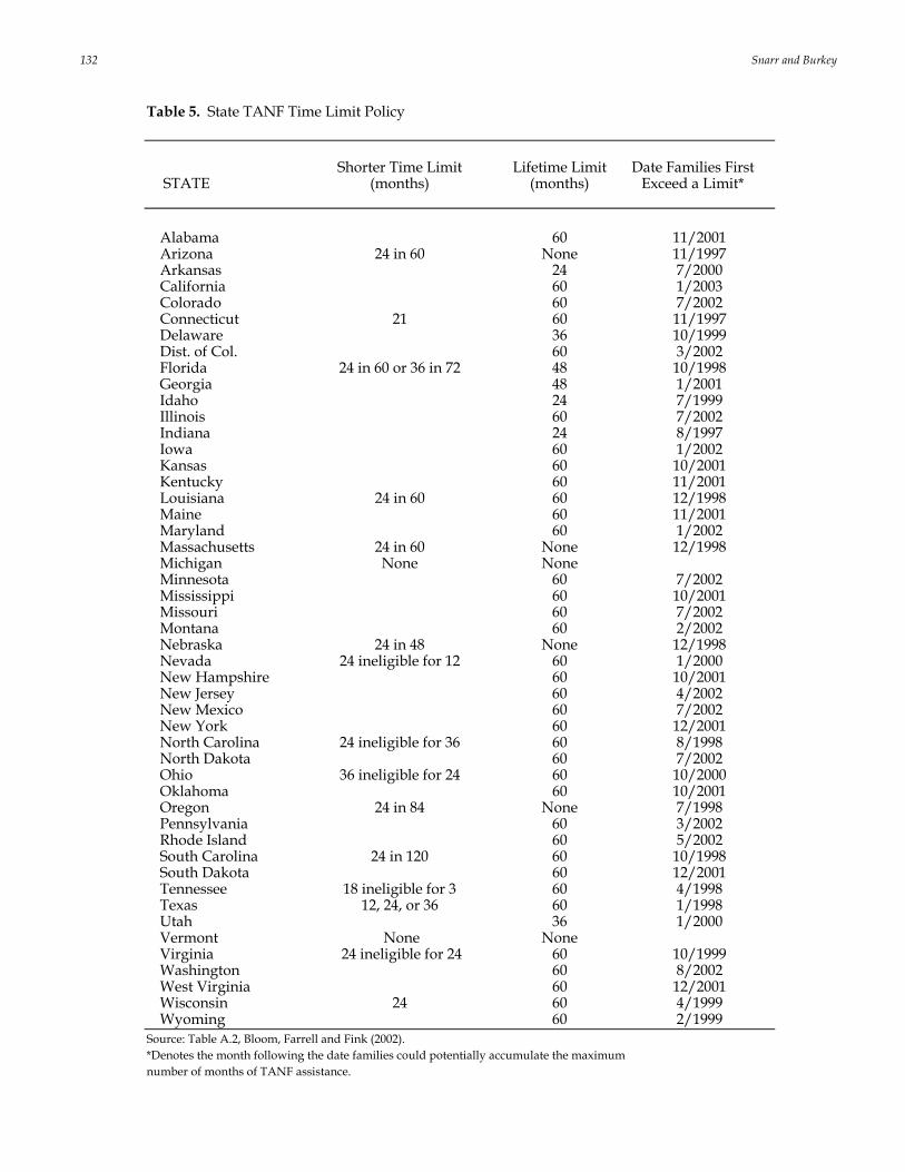
Table 5. State TANF Time Limit Policy

Shorter Time Limit Lifetime Limit Date Families First STATE (months) (months) Exceed a Limit*

Alabama 60 11/2001 Arizona 24 in 60 None 11/1997 Arkansas 24 7/2000 California 60 1/2003 Colorado 60 7/2002 Connecticut 21 60 11/1997 Delaware 36 10/1999 Dist. of Col. 60 3/2002 Florida 24 in 60 or 36 in 72 48 10/1998 Georgia 48 1/2001 Idaho 24 7/1999 Illinois 60 7/2002 Indiana 24 8/1997 Iowa 60 1/2002 Kansas 60 10/2001 Kentucky 60 11/2001 Louisiana 24 in 60 60 12/1998 Maine 60 11/2001 Maryland 60 1/2002 Massachusetts 24 in 60 None 12/1998 Michigan None None Minnesota 60 7/2002 Mississippi 60 10/2001 Missouri 60 7/2002 Montana 60 2/2002 Nebraska 24 in 48 None 12/1998 Nevada 24 ineligible for 12 60 1/2000 New Hampshire 60 10/2001 New Jersey 60 4/2002 New Mexico 60 7/2002 New York 60 12/2001 North Carolina 24 ineligible for 36 60 8/1998 North Dakota 60 7/2002 Ohio 36 ineligible for 24 60 10/2000 Oklahoma 60 10/2001 Oregon 24 in 84 None 7/1998 Pennsylvania 60 3/2002 Rhode Island 60 5/2002 South Carolina 24 in 120 60 10/1998 South Dakota 60 12/2001 Tennessee 18 ineligible for 3 60 4/1998 Texas 12, 24, or 36 60 1/1998 Utah 36 1/2000 Vermont None None Virginia 24 ineligible for 24 60 10/1999 Washington 60 8/2002 West Virginia 60 12/2001 Wisconsin 24 60 4/1999 Wyoming 60 2/1999 Source: Table A.2, Bloom, Farrell and Fink (2002). *Denotes the month following the date families could potentially accumulate the maximum number of months of TANF assistance.


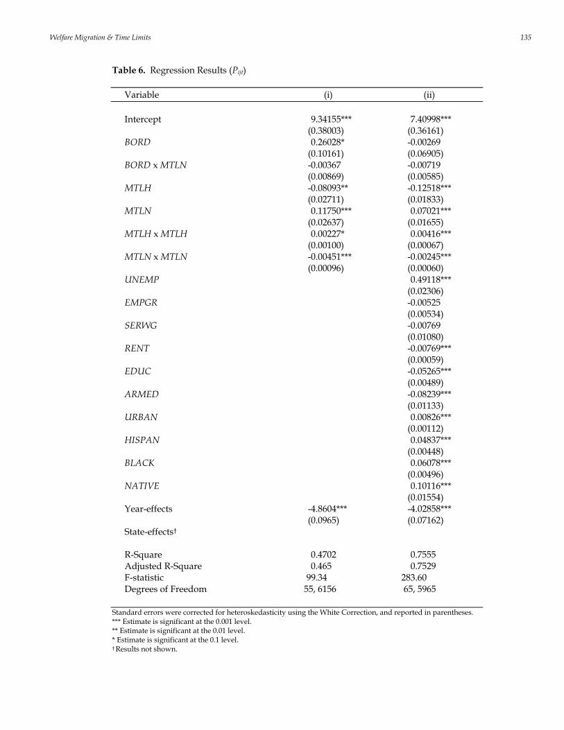
5. Results The empirical estimates of equation (8) are sum-marized in Tables 6 and 7. Column (i) in Table 6 dis-plays the results of estimating equation (8) without the county-level controls (Xit) while column (ii) gives the results with these controls. Both of these regressions were estimated with year-effects and state fixed ef-fects. In addition, the White estimator was used to correct the standard errors for heteroskedasticity (White, 1980). Comparing the results in the two col-umns of Table 6 shows a dramatic improvement in fit when county-level controls are included in the regres-sion. In column (ii) we see that when the control vari-

ables are included, the impact of being a border county becomes much smaller and statistically insig-nificant. In addition, the interaction between the bor-der county dummy and nearest state’s time limit is insignificant in either specification. This outcome most likely results from using border counties as a coarse approximation of migration costs. As seen in Figure 1, migration distances can be very large in the western U.S., even for a typical resident in a border county. In an attempt to more accurately measure mi-gration costs, we calculated the distance of each county’s centroid to the nearest state border (DIST) instead of the border county dummy in subsequent regressions.

Figure 1. Counties along State Borders Additionally, the linear functional form exhibited a high degree of heteroskedasticity, and a residual plot that is indicative of a non-linear functional form (Fig-ure 2). This is common in welfare caseload studies (e.g., Ziliak, Figlio, Davis, and Connolly, 2000; Blank, 2001; McKinnish, 2005). Like our predecessors, we used the logarithm of our dependent variable in our second round of regressions. Comparing Figures 2 and 3 shows a dramatic improvement in the distribu-

tion of the residuals. Column (i) in Table 7 displays the results of estimating the regression explaining the logarithm of the welfare participation rate9 without the county-level controls (Xit) while column (ii) gives the results with these controls. Both of these regres-

9 Six observations from counties with small populations and zero families participating in the welfare program were dropped from the analysis.


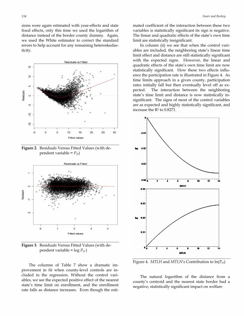
sions were again estimated with year-effects and state fixed effects, only this time we used the logarithm of distance instead of the border county dummy. Again, we used the White estimator to correct the standard errors to help account for any remaining heteroskedas-ticity.

Figure 2. Residuals Versus Fitted Values (with de-

pendent variable = Pijt)

Figure 3. Residuals Versus Fitted Values (with de-

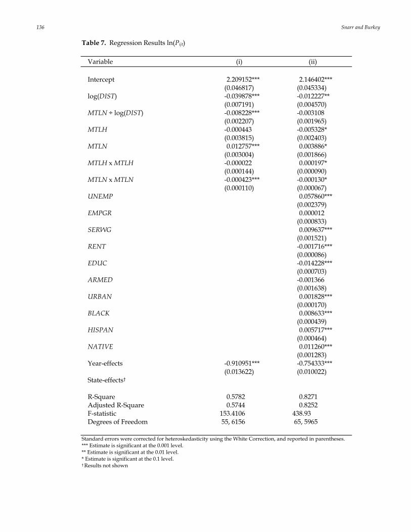
pendent variable = log Pijt ) The columns of Table 7 show a dramatic im-provement in fit when county-level controls are in-cluded in the regression. Without the control vari-ables, we see the expected positive effect of the nearest state’s time limit on enrollment, and the enrollment rate falls as distance increases. Even though the esti-

mated coefficient of the interaction between these two variables is statistically significant its sign is negative. The linear and quadratic effects of the state’s own time limit are statistically insignificant. In column (ii) we see that when the control vari-ables are included, the neighboring state’s linear time limit effect and distance are still statistically significant with the expected signs. However, the linear and quadratic effects of the state’s own time limit are now statistically significant. How these two effects influ-ence the participation rate is illustrated in Figure 4. As time limits approach in a given county, participation rates initially fall but then eventually level off as ex-pected. The interaction between the neighboring state’s time limit and distance is now statistically in-significant. The signs of most of the control variables are as expected and highly statistically significant, and increase the R2 to 0.8271.

Figure 4. MTLH and MTLN’s Contribution to ln(Pjit) The natural logarithm of the distance from a county’s centroid and the nearest state border had a negative, statistically significant impact on welfare


Table 6. Regression Results (Pijt) Variable (i) (ii) Intercept 9.34155*** 7.40998*** (0.38003) (0.36161) BORD 0.26028* -0.00269 (0.10161) (0.06905) BORD x MTLN -0.00367 -0.00719 (0.00869) (0.00585) MTLH -0.08093** -0.12518*** (0.02711) (0.01833) MTLN 0.11750*** 0.07021*** (0.02637) (0.01655) MTLH x MTLH 0.00227* 0.00416*** (0.00100) (0.00067) MTLN x MTLN -0.00451*** -0.00245*** (0.00096) (0.00060) UNEMP 0.49118*** (0.02306) EMPGR -0.00525 (0.00534) SERWG -0.00769 (0.01080) RENT -0.00769*** (0.00059) EDUC -0.05265*** (0.00489) ARMED -0.08239*** (0.01133) URBAN 0.00826*** (0.00112) HISPAN 0.04837*** (0.00448) BLACK 0.06078*** (0.00496) NATIVE 0.10116*** (0.01554) Year-effects -4.8604*** -4.02858*** (0.0965) (0.07162) State-effects† R-Square 0.4702 0.7555 Adjusted R-Square 0.465 0.7529 F-statistic 99.34 283.60 Degrees of Freedom 55, 6156 65, 5965 Standard errors were corrected for heteroskedasticity using the White Correction, and reported in parentheses. *** Estimate is significant at the 0.001 level. ** Estimate is significant at the 0.01 level. * Estimate is significant at the 0.1 level. † Results not shown.


Table 7. Regression Results ln(Pijt)

Variable (i) (ii) Intercept 2.209152*** 2.146402*** (0.046817) (0.045334) log(DIST) -0.039878*** -0.012227** (0.007191) (0.004570) MTLN ÷ log(DIST) -0.008228*** -0.003108 (0.002207) (0.001965) MTLH -0.000443 -0.005328* (0.003815) (0.002403) MTLN 0.012757*** 0.003886* (0.003004) (0.001866) MTLH x MTLH -0.000022 0.000197* (0.000144) (0.000090) MTLN x MTLN -0.000423*** -0.000130* (0.000110) (0.000067) UNEMP 0.057860*** (0.002379) EMPGR 0.000012 (0.000833) SERWG 0.009637*** (0.001521) RENT -0.001716*** (0.000086) EDUC -0.014228*** (0.000703) ARMED -0.001366 (0.001638) URBAN 0.001828*** (0.000170) BLACK 0.008633*** (0.000439) HISPAN 0.005717*** (0.000464) NATIVE 0.011260*** (0.001283) Year-effects -0.910951*** -0.754333*** (0.013622) (0.010022) State-effects† R-Square 0.5782 0.8271 Adjusted R-Square 0.5744 0.8252 F-statistic 153.4106 438.93 Degrees of Freedom 55, 6156 65, 5965 Standard errors were corrected for heteroskedasticity using the White Correction, and reported in parentheses. *** Estimate is significant at the 0.001 level. ** Estimate is significant at the 0.01 level. * Estimate is significant at the 0.1 level. † Results not shown


enrollment. The coefficient of -.012 can be interpreted as an elasticity: A one percent increase in the distance is associated with a .012 percent decrease in welfare enrollment rates. This provides some evidence of wel-fare flipping, as counties closer to a border have in-creased enrollment rates. However, the key interaction term, MTLN ÷ log(DIST) is not statistically significant and of the wrong sign. In this term, we interacted the time limit of the nearest state with 1/log(DIST) because MTLN and DIST are a priori assumed to affect welfare en-rollment in opposite directions. Therefore, a direct interaction would not be appropriate. The own-state and bordering-state time limit in-tensity variables were estimated allowing for the pos-sibility of a nonlinear effect, since one might expect a larger impact on welfare enrollment immediately after a time limit is imposed, with the effect tapering off over time. This is indeed what the estimates suggest. These quadratic functions’ effects on the natural log of the participation rate are graphed in Figure 4.10 The effect of time limits on the own state’s enrollment rate is a fairly steep decline of about 4% in enrollment. However, the effect of a nearby state’s time limit ap-pears to have a more gradual, somewhat smaller off-setting impact on enrollment peaking at around 14 months. This effect of a nearby state’s time limit is ad-ditional evidence supporting the idea of welfare flip-ping. Areas with high unemployment have higher levels of welfare enrollment, but recent growth in the num-ber of jobs created in the service sector appeared to have no impact on welfare enrollment. However, we found some evidence of employment-related migra-tion, as the estimate for Service-Industry wages indi-cates that higher wages may be attracting welfare families who realize that they will likely be required to work as part of the welfare program. However, offset-ting this is the cost of living, as proxied by the median rent paid in the county. The remaining control variables for race, educa-tion, and urbanness all have the expected sign. The variable representing the prevalence of the armed ser-vices in a county was statistically insignificant. The -0.75 coefficient for the year 2000 control variable es-timates that other (unmeasured) effects account for a decrease of approximately 53 percent in welfare en-rollment between 1990 and 2000.

10 To interpret the effect of adding or subtracting a number from the natural log of a dependent variable, calculate eB-1. The result is the proportionate increase in the dependent variable in question.

6. Conclusions The imposition of welfare time limits in some states results in a higher interstate benefit differential for a household nearing a time limit than what existed under AFDC – after a family has run out of benefits in their home state. If the household remains in its home state it cannot receive benefits in the following month. However, if it migrates to a nearby state, it resets its TANF clock because states do not currently share data and cannot impose minimum residency requirements. Thus, the benefit differential is equal to the nearest state’s cash grant. The incentive for time-limit in-duced welfare migration is clear – whether or not people act on this incentive is the issue that we have attempted to ascertain in this paper. Similar to previous research, we found that a state can lower its own welfare enrollment by implement-ing a time limit. However, our finding that this reduc-tion in enrollment may cause spillovers into nearby states is the first of its kind. Finding some evidence of time-limit induced migration and “welfare-flipping” as people move to reenroll in welfare highlights the need for additional research and possible reforms of the system. If time limits are causing families to waste resources by moving rather than returning people to work and self-sufficiency, then the time limits in state TANF programs merely create an inefficiency. Be-cause this is only a preliminary investigation of the existence of time-limit migration, and many states’ time limits had not become binding by the year 2000, there are several ways that this research can be im-proved and extended in the future.

First, continuing to create more accurate variables measuring the cost of moving to another state is likely to improve the accuracy and meaningfulness of the results. Second, because this data is explicitly spatial in nature, the use of spatial regression techniques to de-termine if the coefficients may be biased due to spatial autocorrelation or heterogeneity is advisable. Third, as we mentioned earlier, the use of micro data would be ideal for testing the “welfare-flipping” hypothesis because migration behavior cannot be truly tested with macro data due to ecological inference problems. Lastly, investigators should attempt to include addi-tional policy and descriptive variables in an attempt to simultaneously estimate the possible effects of benefit, amenity, and employment-related migration, in addi-tion to looking for evidence of time-limit induced mi-gration.


Acknowledgement

An early version of this paper was presented at

the 2006 annual meeting of the Southern Regional Sci-ence Association, April 2, St. Augustine, FL. The au-thors are grateful for the helpful comments from Brian Cushing, Mark Partridge, participants of the SRSA meetings, and an anonymous reviewer. All remaining errors are our own.

References Blank, Rebecca. 1988. The effect of welfare and wage

levels on the location decisions of female-headed households. Journal of Urban Economics 24(2): 186-211.

Blank, Rebecca. 2001. What causes public assistance caseloads to grow? Journal of Human Resources 36(1): 85-118.

Bloom, Dan, Mary Farrell, and Barbara Fink with Diana Adams-Ciardullo. 2002. Welfare Time Limits State Policies, Implementation, and Effects on Families. Manpower Demonstration Research Corporation.

Borjas, George. 1998. Immigration and welfare mag-nets. NBER Working Paper No. W6813.

Brown, Charles C., and Wallace E. Oates. 1987. Assis-tance to the poor in a Federal system. Journal of Public Economics 32(3): 307-330.

Brueckner, Jan K. 2000. Welfare reform and the race to the bottom: Theory and evidence. Southern Eco-nomic Journal 66(3): 505-525.

Burkey, Mark L. and Scott P. Simkins. 2004. Factors affecting the location of payday lending and tradi-tional banking services in North Carolina. Review of Regional Studies 34(2): 191-205.

De Jong, Gordon, Deborah Roempke Graefe, and Tanja St. Pierre. 2005. Welfare reform and inter-state migration of poor families. Demography. 42(3): 469-497.

Enchautegui, Maria E. 1997. Welfare payments and other economic determinants of female migration. Journal of Labor Economics 15(3): 529-554.

Fang, Hanming, and Michael P. Keane. 2004. Assess-ing the impact of welfare reform on single moth-ers. Brookings Papers on Economic Activity.

Greene, William H. 2000. Econometric Analysis, 4th ed. New Jersey: Prentice Hall.

Grogger, Jeffery T. 2003. The effect of time limits, the EITC, and the other policy changes on welfare use, work, and income among female-headed families. Review of Economics and Statistics 85(2): 394-408.

Grogger, Jeffery T. 2004a. Time limits and welfare use. The Journal of Human Resources 39(2): 405-424.

Grogger, Jeffery T. 2004b. Welfare transitions in the

1990s: The economy, welfare policy, and the EITC. Journal of Policy Analysis and Management 23(4): 671-698.

Grogger, Jeffery T., Lynn A. Karoly and Jacob A. Klerman. 2002. Consequences of Welfare Reform: A Research Synthesis. Document DRU-2676-DHHS, Prepared by RAND for the Agency for Children and Families, U.S. Department of Health and Hu-man Services. Santa Monica, CA: RAND.

Grogger, Jeffery T. and Charles Michalopoulos. 2003. Welfare dynamics under time limits. Journal of Po-litical Economy 111(3): 530-554.

Gramlich, Edward M. and Deborah S. Laren. 1984. Migration and income redistribution responsibili-ties. The Journal of Human Resources 19(4): 489-511.

Kaestner, Robert, Neeraj Kaushal and Gregg Van Ryzin. 2003. Migration consequences of welfare reform. Journal of Urban Economics 53(3): 357-376.

Kaushal, Neeraj and Robert Kaestner. 2001. From welfare to work: Has welfare reform worked? Journal of Policy Analysis and Management 20(4): 699-719.

Lindert, Kathy. 2005. Implementing Means-tested Wel-fare Systems in the United States. Social Protection Unit, Human Development Network, The World Bank, Social Protection Discussion Paper Series No. 0532.

Levine, Phillip B. and David J. Zimmerman. 1995. An Empirical Analysis of the Welfare Magnet Debate Us-ing the NLSY. NBER Working Paper No. 5264.

McKinnish, Terra. 2005. Importing the poor: Welfare magnetism and cross-border welfare migration. The Journal of Human Resources 40(1): 57-76.

Meyer, Bruce. D. 1998. Do the Poor Move to Receive Higher Welfare Benefits? Working Paper, North-western University, Department of Economics and Institute for Policy Research.

Rosenheim, Margaret. 1970. The constitutionality of durational residence requirements. Social Service Review 44: 82-93

Southwick, Lawrence Jr. 1981. Public welfare pro-grams and recipient migration. Growth and Change 12(4): 22-32.

Snarr, Hal W. and Dan Axelsen. 2006. Welfare Dynam-ics: A Counter Argument to the Forward-Looking Con-jecture. Working Paper available from the lead au-thor.

Stegman, Michael A. and Faris, Robert. 2003. Payday lending: A business model that encourages chronic borrowing. Economic Development Quar-terly 17(1): 8-32.


Swann, Christopher A. 2005. Welfare reform when recipients are forward-looking. The Journal of Hu-man Resources 40(1): 31-56.

Walker, James. 1994. Migration among Low-Income Households: Helping the Witch Doctors Reach Consen-sus. Working Paper.

Wildasin, David E. 1991. Income redistribution in a common labor market. American Economic Review. 81(4): 757-774.

White, Halbert. 1980. A heteroscedasticity-consistent covariance matrix estimator and a direct test for heteroscedasticity. Econometrica 48(4): 817-838.

U. S. Department of Health and Human Services. 2000a. Welfare Reform Information Technology: A Study of Issues in Implementing Information Systems for the Temporary Assistance for Needy Families (TANF) Program. Washington, D.C.: DHHS.

U. S. Department of Health and Human Services. 2000b. Temporary Assistance for Needy Families (TANF) Program, Third Annual Report to Congress. Washington, D.C.: DHHS.

U.S. Department of Health, Education, and Welfare. 1969. Characteristics of State Public Assistance Plans Under the Social Security Act, 1967. Washington, DC: U.S. Government Printing Office.

U.S. House of Representatives, Committee on Ways and Means. 2000. The 2000 Green Book: Background Material and Data on Programs Within the Jurisdic-tion of the Committee on Ways and Means. Washing-ton, D.C.: U.S. Government Printing Office.

Ziliak, James, David Figlio, Elizabeth Davis, and Laura Connolly. 2000. Accounting for the decline in AFDC caseloads: Welfare reform or the economy. Journal of Human Resources 35(3): 570-586.

Appendix

Proof of PROPOSITION 1: The household migrates if 1Ev exceeds 0

Ev , which is equivalent to

( ) ( ) ( ) ( )ln (1) ln (1) ln (0) ln (0)E E E Ec c c cβ β+ > +

( ) ( )(1 ) ln (1) (1 ) ln (0)E Ec cβ β+ > +

(1) (0)E Ec c>

( ) ( ) ( )n nG wh G G w h wh d F G wh G wh G whκ β β β+ + − + − − − + + > + + +

n nG G w h wh F dκ− + − − >

n nG G w h wh Fd

d− + − −

<

Proof of PROPOSITION 2: The proof of Proposition 2 follows the proof above.

A preliminary investigation of welfare migration induced by time limits (Mark L. Burkey)

Documents

Transcript of A preliminary investigation of welfare migration induced by time limits (Mark L. Burkey)