A parallel method for time discretization of parabolic equations based on Laplace transformation and...
19
MATHEMATICS OF COMPUTATION Volume 69, Number 229, Pages 177–195 S 0025-5718(99)01098-4 Article electronically published on April 7, 1999 A PARALLEL METHOD FOR TIME-DISCRETIZATION OF PARABOLIC PROBLEMS BASED ON CONTOUR INTEGRAL REPRESENTATION AND QUADRATURE DONGWOO SHEEN, IAN H. SLOAN, AND VIDAR THOM ´ EE Abstract. We treat the time discretization of an initial-value problem for a homogeneous abstract parabolic equation by first using a representation of the solution as an integral along the boundary of a sector in the right half of the complex plane, then transforming this into a real integral on the finite interval [0, 1], and finally applying a standard quadrature formula to this integral. The method requires the solution of a finite set of elliptic problems with complex coefficients, which are independent and may therefore be done in parallel. The method is combined with spatial discretization by finite elements. 1. Introduction We consider the initial-value problem u t + Au =0, for t> 0, with u(0) = u 0 , (1.1) where A is a symmetric, positive definite operator with a compact inverse, defined on a dense subset D of a Hilbert space H , with inner product (·, ·). The solution may be written in the form (cf. [8], Theorem 1.7.7) u(t)= 1 2πi Z Γ e -zt R(z ; A)u 0 dz, for t> 0, (1.2) where R(z ; A)=(A - zI ) -1 is the negative of the resolvent of A, and Γ is a conveniently chosen path in the right half plane. With the minimal eigenvalue of A bounded below by λ 0 > 0, and with 0 ≤ γ<λ 0 , we shall use Γ = Γ γ = {z = γ + σ ± iσ; σ ≥ 0}, with Im z increasing from -∞ to ∞. This representation may be obtained by applying the Laplace transform, defined by w(z )=ˆ u(z )= Z ∞ 0 e zt u(t) dt, for Re z ≤ γ, (1.3) to the initial value problem (1.1). In this way we derive Aw - zw = u 0 , i.e., w(z )= R(z ; A)u 0 , for Re z ≤ γ, (1.4) Received by the editor March 26, 1998. 1991 Mathematics Subject Classification. Primary 65M12, 65M15, 65M99. This work was partially supported by the Australian Research Council and the Korea Sci- ence & Engineering Foundation through the Global Analysis Research Center at Seoul National University. c 1999 American Mathematical Society 177
Transcript of A parallel method for time discretization of parabolic equations based on Laplace transformation and...

MATHEMATICS OF COMPUTATIONVolume 69, Number 229, Pages 177–195S 0025-5718(99)01098-4Article electronically published on April 7, 1999
A PARALLEL METHODFOR TIME-DISCRETIZATION OF PARABOLIC PROBLEMS
BASED ON CONTOUR INTEGRAL REPRESENTATIONAND QUADRATURE
DONGWOO SHEEN, IAN H. SLOAN, AND VIDAR THOMEE
Abstract. We treat the time discretization of an initial-value problem for ahomogeneous abstract parabolic equation by first using a representation of thesolution as an integral along the boundary of a sector in the right half of thecomplex plane, then transforming this into a real integral on the finite interval[0, 1], and finally applying a standard quadrature formula to this integral. Themethod requires the solution of a finite set of elliptic problems with complexcoefficients, which are independent and may therefore be done in parallel. Themethod is combined with spatial discretization by finite elements.
1. Introduction
We consider the initial-value problem
ut +Au = 0, for t > 0, with u(0) = u0,(1.1)
where A is a symmetric, positive definite operator with a compact inverse, definedon a dense subset D of a Hilbert space H , with inner product (·, ·). The solutionmay be written in the form (cf. [8], Theorem 1.7.7)
u(t) =1
2πi
∫Γ
e−ztR(z;A)u0 dz, for t > 0,(1.2)
where R(z;A) = (A − zI)−1 is the negative of the resolvent of A, and Γ is aconveniently chosen path in the right half plane. With the minimal eigenvalue ofA bounded below by λ0 > 0, and with 0 ≤ γ < λ0, we shall use Γ = Γγ = z =γ + σ ± iσ;σ ≥ 0, with Im z increasing from −∞ to ∞. This representation maybe obtained by applying the Laplace transform, defined by
w(z) = u(z) =∫ ∞
0
eztu(t) dt, for Re z ≤ γ,(1.3)
to the initial value problem (1.1). In this way we derive
Aw − zw = u0, i.e., w(z) = R(z;A)u0, for Re z ≤ γ,(1.4)
Received by the editor March 26, 1998.1991 Mathematics Subject Classification. Primary 65M12, 65M15, 65M99.This work was partially supported by the Australian Research Council and the Korea Sci-
ence & Engineering Foundation through the Global Analysis Research Center at Seoul NationalUniversity.
c©1999 American Mathematical Society
177
178 DONGWOO SHEEN, IAN H. SLOAN, AND VIDAR THOMEE
and then retrieve u(t) by the inverse of the Laplace transform (1.3) taken alongz; Re z = γ, subsequently deforming this path to Γγ . This is possible sincew(z) = R(z;A)u0 exists for z ∈ C \ [λ0,∞), and since ‖R(z;A)‖ ≤ C(|z| + 1)−1
for z bounded away from [λ0,∞). Since A is self-adjoint the representation (1.2)may also be established by deforming Γ into a union of small circles around theeigenvalues of A, in which case (1.2) reduces to the eigenfunction expansion of u(t).
The contour integral representation (1.2) of u(t) may be written as
u(t) =∫ ∞
0
e−(γ+σ)tg(t;σ) dσ,(1.5)
where
g(t;σ) =1
2πi(νe−iσtw(γ + νσ)− νeiσtw(γ + νσ)
), with ν = 1 + i.(1.6)
In our applications w will be a complex-valued function, satisfying w(z) = w(z)because of (1.4), in which case g(t;σ) is real, and
g(t;σ) =1π
Im(νe−iσtw(γ + νσ)
).(1.7)
Our approach to the approximate solution of (1.1) is to apply a quadraturescheme to (1.5). We shall later also apply our method to the discretization intime of an initial value problem of the form (1.1) which has been obtained from aninitial boundary value problem for a parabolic partial differential equation by firstdiscretizing in the space variables by finite elements.
We consider quadrature approximations to the integral in (1.5) of the form
U(t) =∑
j
ωj(t)g(t;σj), for t > 0,(1.8)
with non-negative quadrature points σj and positive quadrature weights ωj(t). Theconstruction of such a quadrature rule will be accomplished by first changing thevariable in (1.5) to y = e−ασt, where α is a positive number to be specified later,obtaining
u(t) =e−γt
αt
∫ 1
0
y−1+1/αg(t;σ(y)) dy, with σ(y) =1αt
log1y,(1.9)
and then applying a standard quadrature rule. For simplicity, our first approxi-mation uses the composite trapezoidal rule based on a uniform partition of [0, 1],0 = y0 < y1 < · · · < yN = 1, where yj = j/N, j = 0, · · · , N. We recall that for theintegral If =
∫ 1
0 f(y) dy the composite trapezoidal rule is
TNf =1
2N(f(y0) + 2f(y1) + 2f(y2) + · · ·+ 2f(yN−1) + f(yN )
),(1.10)
and that the quadrature error satisfies (see [1], p. 220)
|TNf − If | ≤ 18N2
∫ 1
0
|f ′′(y)| dy.(1.11)
Applying this with f(y) = (αt)−1y−1+1/αg(t;σ(y)), we get a quadrature rule of theform (1.8), with
σj =1αt
log1yj
=1αt
logN
j, j = 0, . . . , N,(1.12)

TIME-DISCRETIZATION OF PARABOLIC PROBLEMS 179
and the corresponding weights (except the first and the last, which have an addi-tional factor of 1
2 ) are
ωj(t) =e−γt
αtNy−1+1/αj =
e−γt
αtN(j
N)−1+1/α.(1.13)
The positive number α is then chosen so as to make the error bound in (1.11) small.It turns out, as we shall see below, that
‖f ′′(y)‖ ≤ C(α, t)y−3+1/α‖u0‖, for y ∈ [0, 1],
and hence the integral in the vector version of (1.11) is finite for α < 1/2, so thatthe error in that situation is of optimal order O(N−2).
Assume now that the solution is sought for t > τ , where τ is a positive numberchosen by the user. For the method to be efficient it is crucial that the same set ofpoints σj be used for a whole range of t values. Since the σj depend on α and t onlythrough the product αt, this product should thus be held constant in a time interval[τ, T ], implying that α must vary with t. In view of the above it is natural to basethe choice of the σj on αt = 1
2τ, or α = 12τ/t, because t > τ is then equivalent to
α < 1/2.Having thus fixed τ and chosen α = 1
2τ/t, thereby securing O(N−2) convergencefor each t > τ , we may still ask for the properties of the method for t ≤ τ , orfor α ≥ 1/2. Since f(y0) = f(0) = 0 if α < 1 because g(t;σ) is bounded, thequadrature point at y = 0 (corresponding to σ = ∞) does not contribute to thequadrature sum for α < 1. If α ≥ 1, we define the quadrature sum so as to omitthe y = 0 term; that is, we “ignore the singularity” (see [1], Section 2.12.7) inthe situation in which there is an endpoint singularity. Thus our quadrature sumsalways run only from j = 1 to j = N . With this understanding we shall be ableto show error estimates for 0 < t ≤ τ which are of lower order than O(N−2); theorder is O(N−2t/τ ) for 0 < t < τ , with an additional factor log logN when t = τ .A full statement is in Theorem 2.2.
Thus, the definition of our method may be summarized as follows: We firstchoose γ ∈ [0, λ0) and the threshold τ > 0, then for t and α satisfying αt = 1
2τ
we determine σj = 2τ−1 log(N/j), j = 1, . . . , N, then solve the N complex-valuedelliptic problems (1.4) with z = γ + νσj , ν = 1 + i, and finally form g(t;σj) andU(t) = Uτ (t) from (1.8), (1.6), and (1.13). In the fully discrete case the ellipticproblems (1.4) are solved approximately by the finite element method.
Instead of the trapezoidal rule we can apply the composite Simpson rule (pro-vided N is even),
SNf =1
3N(f(y0) + 4f(y1) + 2f(y2) + 4f(y3) + · · ·+ 4f(yN−1) + f(yN)
),(1.14)
with the error estimate
|SNf − If | ≤ C
N4
∫ 1
0
|f (iv)(y)| dy.(1.15)
In this case it turns out, as we shall see, that the full O(N−4) convergence order isobtained only for α < 1
4 , and it is then appropriate to choose α so that αt = 14τ, to
secure again the full order of convergence for t > τ . Once more convergence ratesof lower orders may be shown for t ≤ τ . The full Simpson’s rule result is stated asTheorem 2.3.

180 DONGWOO SHEEN, IAN H. SLOAN, AND VIDAR THOMEE
We now turn to discretization in both space and time of an initial boundary valueproblem for a parabolic partial differential equation. For simplicity we consider thecase of the heat equation, viz.
ut −∆u = 0 in Ω, with u = 0 on ∂Ω, for t > 0,
u(·, 0) = u0 in Ω,(1.16)
where Ω ⊂ Rd is a domain with smooth boundary ∂Ω. We thus choose the Hilbertspace H as L2(Ω) with (v, w) =
∫Ω v(x)w(x) dx. Here A = −∆, the Laplacian,
which is defined in D(A) = H2(Ω) ∩H10 (Ω). Setting
A(v, z) =∫
Ω
∇v(x) · ∇z(x) dx,
and letting Vh denote piecewise linear finite element subspaces with standard prop-erties, the finite element approximation wh(z) ∈ Vh of the solution w of (1.4)satisfies
A(wh, χ)− z(wh, χ) = (u0, χ), ∀χ ∈ Vh, for z /∈ [λ0,∞).(1.17)
The semidiscrete approximation uh(t) ∈ Vh to (1.1) is defined by
(uh,t, χ) +A(uh, χ) = 0, ∀χ ∈ Vh, for t > 0, with uh(0) = Phu0,(1.18)
where Ph denotes the orthogonal projection in L2(Ω) onto Vh. Defining the discreteanalogue Ah : Vh → Vh of A = −∆ by
(Ahψ, χ) = A(ψ, χ), ∀ψ, χ ∈ Vh,
we see that (1.18) is of the form (1.1) with A replaced by Ah. Similarly, (1.17) isof the form (1.4). It may be proved, analogously to (1.2) and (1.5), that
uh(t) =1
2πi
∫Γ
e−ztwh(z) dz =∫ ∞
0
e−(γ+σ)tgh(t;σ) dσ,
where (cf. (1.7)) gh(t;σ) = Im(νe−iσtwh(γ+ νσ))/π. Our fully discrete approxima-tion Uh(t) is then obtained by application of the quadrature approximation (1.8)to this integral, so that
Uh(t) =N∑
j=1
ωj(t)gh(t;σj).(1.19)
It will follow from our main result that in the trapezoidal rule case ‖Uh(t)−uh(t)‖ =O(N−2) for t > τ , uniformly in h, with lower orders of convergence for t ≤ τ .Together with the known estimate ‖uh(t) − u(t)‖ = O(h2) for t > 0, this will givea complete error estimate of order O(N−2 + h2) for the fully discrete problem inthis case (see Section 3). Similarly, in the Simpson rule case the complete errorestimate is of order O(N−4 + h2).
The error bounds to be shown later limit the range of t-values that can effectivelybe covered with fixed quadrature points σj ; for example, for γ = 0 we shall see thatrestriction to an interval τ ≤ t ≤ 2τ might be appropriate, while for γ > 0 a largerinterval could be suitable – see Tables 1-3 and associated discussion. The errorbounds will also show that this is not a method of preference for small times t.
We remark that our method is introduced and studied so far only for a homoge-neous parabolic equation. However, the initial value problem for the inhomogeneous

TIME-DISCRETIZATION OF PARABOLIC PROBLEMS 181
equation,
ut +Au = f, for t > 0, with u(0) = u0,(1.20)
in the special case in which f is independent of time, may be reduced to an initial-value problem of the form (1.1). In fact, let u∞ denote the stationary solution of(1.20) defined by Au∞ = f . Then the solution of (1.20) may be written u(t) =u∞ + v(t), where
vt +Av = 0, for t > 0, with v(0) = u0 − u∞,
and our method may be applied to determine v(t).In the finite element application to this problem it is natural to take as discrete
initial values vh(0) = Phu0 − Thf , where Th = A−1h Ph, with Ah and Ph as above.
This differs from the initial value suggested by (1.18), which is Ph(u0 − u∞), byThf − Phu∞ = (Th − PhT )f, where T = A−1. By the stability of the solutionoperator for the homogeneous semidiscrete equation the contribution to the errorof this difference is bounded by Ch2e−λ0t‖f‖, see, e.g., [10].
In the title we described this as a parallel method. The reason is clear fromthe formula (1.19). To compute Uh(t) for a range of times t ≥ τ we need tosolve the finite element problems (1.17) for z = γ + νσj , j = 1, . . . , N . Theseproblems are completely independent, and can therefore be computed on separateprocessors, with no need for shared memory. In contrast, the normal step-by-steptime-marching methods for parabolic problems are not easily parallelizable.
Our method, like the method of eigenfunction expansion, requires that the op-erator A be independent of time and symmetric positive definite. However, therepresentation (1.2) is valid for more general operators A that generate analyticsemigroups, and our time discretization method naturally extends to this case; weplan to return to the analysis of such problems on a later occasion.
Numerical methods for inhomogeneous parabolic and hyperbolic equations basedon the use of Fourier transformation have been considered in [2], [3], [7], and [9], andprovided the starting point for the present work. For other methods for parabolicequations of non-timestepping type, see, e.g., [11, Chapter 9], [5], and [6].
2. Analysis of the quadrature scheme
We recall that in addition to (1.2) the solution of (1.1) admits the representation
u(t) = E(t;A)u0 =∞∑
l=1
e−λlt(u0, ϕl)ϕl,
where ϕl∞l=1 and λl∞l=1 are a basis of orthonormal eigenfunctions and corre-sponding eigenvalues of A, and where E(t;A) = e−At is the semigroup generatedby −A. Similarly, the approximate solution defined by (1.8) and (1.6) may beexpressed as
U(t) = Q(t;A)u0 =∞∑
l=1
Q(t;λl)(u0, ϕl)ϕl,(2.1)
where Q(t;A) is a rational function of A, viz.
Q(t;A) =N∑
j=1
ωj(t)1π
Im(νe−iσj tR(γ + νσj ;A)
);

182 DONGWOO SHEEN, IAN H. SLOAN, AND VIDAR THOMEE
recall that the imaginary part of a bounded linear operator B on the Hilbert spaceH is defined by ImB = (B −B∗)/(2i). This makes it possible below to reduce theproofs of the stability and error estimates to the scalar case
u′ + λu = 0, for t > 0, with u(0) = 1.(2.2)
We suppose first that the time discretization is accomplished by the trapezoidalrule, and show the following stability property of our time discretization operator.
Proposition 2.1. Let τ > 0, and assume that the eigenvalues of A are boundedbelow by λ0, and let 0 ≤ γ < λ0. Let U(t) = Q(t;A)u0 be the N -point trapezoidalrule approximation to (1.9), with g(t;σ) given by (1.6), and with αt = 1
2τ . Thenthere is a constant C independent of t and τ such that, with log+ x = max(log x, 0),
‖U(t)‖ = ‖Q(t;A)u0‖ ≤ Ce−γt( 11 + t
+ log+
1t
+1τ
1Nmin(1,2t/τ)
)‖u0‖, t > 0.
Proof. It suffices to show this for the scalar problem (2.2), with a constant Cindependent of λ ≥ λ0. In fact, by (2.1),
‖Q(t;A)u0‖ =( ∞∑
l=1
Q(t;λl)2(u0, ϕl)2)1/2 ≤ max
l|Q(t;λl)| ‖u0‖,
so it suffices to show that
|Q(t;λ)| ≤ Ce−γt( 11 + t
+ log+
1t
+1τ
1Nmin(1,2t/τ)
)for λ ≥ λ0,(2.3)
where it follows from the expression above that
Q(t;λ) =N∑
j=1
ωj(t)1π
Im(νe−iσj t(λ− γ − νσj)−1).
Recalling that ν = 1 + i, we have, for λ ≥ λ0 > γ ≥ 0, with C = C(λ0 − γ),
1π| Im(νe−iσt(λ− γ − νσ)−1)| ≤ C|λ− γ − νσ|−1 ≤ C(σ + 1)−1.
Hence
|Q(t;λ)| ≤ CN∑
j=1
ωj(t)(σj + 1)−1 ≤ Ce−γt
αtN
N∑j=1
y−1+1/αj (σ(yj) + 1)−1 = Ce−γtJN ,
where JN is a Riemann sum for the first integral in
J =1αt
∫ 1
0
y−1+1/α(σ(y) + 1)−1 dy =∫ ∞
0
e−σt(σ + 1)−1 dσ.
For α ≤ 1, i.e., for t ≥ 12 τ , the function y−1+1/α(σ(y) + 1)−1 is increasing from 0
to 1 as y increases from 0 to 1, and therefore the sum of the first N − 1 terms ofJN is bounded by J , so that
JN ≤ J +1
αtN= J +
2τ N
.
The bound (2.3) is therefore proved for 2t/τ ≥ 1 by
J = et
∫ ∞
t
e−x
xdx ≤ C
1 + log 1
t , t ≤ 11t , t ≥ 1
≤ C
( 11 + t
+ log+
1t
).(2.4)

TIME-DISCRETIZATION OF PARABOLIC PROBLEMS 183
It remains to bound JN when α > 1, i.e., to prove (2.3) for 2t/τ < 1. We thenneed to handle the product of the decreasing function y−1+1/α and the increasingfunction (σ(y) + 1)−1. For this purpose we first show that
(σ(yj) + 1)−1 ≤ C(σ(yj−1) + 1)−1, for 2 ≤ j ≤ N − 1,(2.5)
with C independent of j and N , from which it will follow for 2 ≤ j ≤ N − 1 that
N−1y−1+1/αj (σ(yj) + 1)−1 ≤ CN−1y
−1+1/αj (σ(yj−1) + 1)−1
≤ C
∫ yj
yj−1
y−1+1/α(σ(y) + 1)−1 dy,
and hence, by summation of this bound over j = 2, . . . , N − 1,
JN ≤ C(J +
1τ N1/α
+1τ N
)≤ C
(J +
1τ
1Nmin(1,2t/τ)
).
Since σ(y) = 2 log(1/y)/τ , the claim (2.5) is equivalent to showing the bounded-ness of (log(1/yj−1) + τ/2)/(log(1/yj) + τ/2) for τ ≥ 0, 2 ≤ j ≤ N , or (since thisratio takes its maximum value at τ = 0) that ϕ(y) = log(y − k)/ log y is boundedin [2k, 1 − k], where k = 1/N . But ϕ(y) → ∞ when y → k and y → 1. It thensuffices to show that ϕ(2k) and ϕ(1 − k) are bounded, and that ϕ(y) has only onestationary point in (2k, 1− k) (which then has to be a minimum). We have
ϕ(2k) =logN
log(N/2)≤ log 3
log(3/2), for N ≥ 3,
and
ϕ(1− k) =log(1− 2k)log(1− k)
= 2 +O(1N
), as N →∞,
so that both ϕ(2k) and ϕ(1 − k) are bounded for N ≥ 3. A stationary point y ofϕ(y) has to satisfy (y − k)−1 log y − y−1 log(y − k) = 0, or g(y) = g(y − k), whereg(y) = y log y. But g(0) = g(1) = 0, g(y) < 0 for y ∈ (0, 1), and g′(y) = 0 only fory = e−1, so that g(y) = g(y − k) has exactly one solution in (k, 1) for k < 1. Thusthe claim is established, and the proof is complete.
Note that the stability bound contains a term with a factor τ−1, and thus is notuniformly bounded for small τ .
Let us remark that, with a slightly modified definition of the approximate so-lution U(t), and with a mild regularity assumption on u0, it is possible to showuniform boundedness of the time discrete solution as t tends to 0 for fixed τ > 0.In fact, writing instead of (1.2) for the exact solution
u(t) =1
2πi
∫Γγ
e−zt(1 + z)−εR(z;A) (I +A)εu0 dz, with ε > 0,
we may define an approximate solution Uε(t) by
Uε(t) = Qε(t;A)(I +A)εu0,
where
Qε(t;A) =N∑
j=1
ωj(t)1π
Im(νe−iσjt(1 + γ + νσj)−εR(γ + νσj ;A)
).

184 DONGWOO SHEEN, IAN H. SLOAN, AND VIDAR THOMEE
With this choice we first have to apply (I +A)ε to the given initial data; for ε = 1this simply entails application of A. Similarly to our earlier estimate, we find inthe scalar case A = λ that
|Qε(t;λ)| ≤ e−γt
αtN
N∑j=1
y−1+1/αj (σj + 1)−1−ε
≤ Ce−γt( ∫ ∞
0
e−tσ(σ + 1)−1−ε dσ +1τ
1Nmin(1,2t/τ)
)≤ Ce−γt
( 11 + t
+1τ
1Nmin(1,2t/τ)
).
Thus, in this case, since (I +A)εA−ε is bounded in H ,
‖Uε(t)‖ ≤ Ce−γt( 11 + t
+1τ
1Nmin(1,2t/τ)
)‖Aεu0‖, for t ≥ 0,
in which there is no longer any logarithmic behavior as t→ 0.We now return to the main theme and show an error estimate for the approximate
solution U(t) defined by the trapezoidal rule.
Theorem 2.2. Let τ > 0 and assume the eigenvalues of A are bounded below byλ0, and let 0 ≤ γ < λ0. Assume that the quadrature approximation U(t) is obtainedby applying the trapezoidal rule (1.10) (with the y0 term omitted) to the integral in(1.9), where g(t;σ) is defined by (1.6), and α is chosen so that αt = τ/2. Thenthere exists C = C(λ0 − γ) > 0, such that
‖U(t)− u(t)‖ ≤ C‖u0‖e−γt
1N2
( 1 + t2
τ2(1 + t− τ)+t2
τ2log+
1t− τ
), t > τ,
1N2
(log logN +
1τ2
+ log+
1τ
), N ≥ 3, t = τ,
1N2t/τ
(1 + τ2
τ2+ log+
1τ − t
+ log+
1t
), 0 < t < τ.
Proof. Again it suffices to consider the scalar problem (2.2), since it follows in thesame way as in the proof of Proposition 2.1 that
‖U(t)− u(t)‖ ≤ maxl|Q(t;λl)− e−λlt| ‖u0‖.
Thus it is sufficient to show that the modulus of the scalar quadrature error ε(t;λ) =|Q(t;λ) − e−λt| can be estimated as in the theorem (with ‖u0‖ = 1) for λ ≥ λ0.Recall that the trapezoidal rule has the error bound (1.11). Therefore, recallingthat ν = 1 + i and σ(y) = 2τ−1 log(1/y), we have
ε(t;λ) ≤ e−γt
8N2
∫ 1
0
|f ′′(y)| dy,
where, from (1.9) and (1.6),
f(y) = 2(πτ)−1y−1+1/α Im(νe−iσ(y)tw(γ + νσ(y)), with w(z) = (λ− z)−1.
To bound the integral, we write, using −σ(y)t = log y/α,
f(y) = 2(πτ)−1 Im(νF (y)), where F (y) = y−1+ν/αW (y), W (y) = w(γ + νσ(y)),
and find that
F ′′(y) = y−3+ν/α((−1 +
ν
α)(−2 +
ν
α)W (y) + 2(−1 +
ν
α)yW ′(y) + y2W ′′(y)
).
TIME-DISCRETIZATION OF PARABOLIC PROBLEMS 185
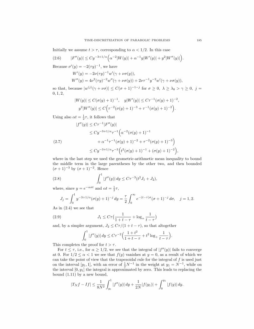
Initially we assume t > τ , corresponding to α < 1/2. In this case
|F ′′(y)| ≤ Cy−3+1/α(α−2|W (y)|+ α−1y|W ′(y)|+ y2|W ′′(y)|
).(2.6)
Because σ′(y) = −2(τy)−1, we have
W ′(y) = −2ν(τy)−1w′(γ + νσ(y)),
W ′′(y) = 4ν2(τy)−2w′′(γ + νσ(y)) + 2ντ−1y−2w′(γ + νσ(y)),
so that, because |w(j)(γ + νσ)| ≤ C(σ + 1)−1−j for σ ≥ 0, λ ≥ λ0 > γ ≥ 0, j =0, 1, 2,
|W (y)| ≤ C(σ(y) + 1)−1, y|W ′(y)| ≤ Cτ−1(σ(y) + 1)−2,
y2|W ′′(y)| ≤ C(τ−2(σ(y) + 1)−3 + τ−1(σ(y) + 1)−2
).
Using also αt = 12τ , it follows that
|f ′′(y)| ≤ Cτ−1|F ′′(y)|≤ Cy−3+1/ατ−1
(α−2(σ(y) + 1)−1
+ α−1τ−1(σ(y) + 1)−2 + τ−2(σ(y) + 1)−3)
(2.7)
≤ Cy−3+1/ατ−3(t2(σ(y) + 1)−1 + (σ(y) + 1)−2
),
where in the last step we used the geometric-arithmetic mean inequality to boundthe middle term in the large parentheses by the other two, and then bounded(σ + 1)−3 by (σ + 1)−2. Hence∫ 1
0
|f ′′(y)| dy ≤ Cτ−3(t2J1 + J2),(2.8)
where, since y = e−ασt and αt = 12τ ,
Jj =∫ 1
0
y−3+1/α(σ(y) + 1)−j dy =τ
2
∫ ∞
0
e−(t−τ)σ(σ + 1)−j dσ, j = 1, 2.
As in (2.4) we see that
J1 ≤ Cτ( 11 + t− τ
+ log+
1t− τ
)(2.9)
and, by a simpler argument, J2 ≤ Cτ/(1 + t− τ), so that altogether∫ 1
0
|f ′′(y)| dy ≤ Cτ−2( 1 + t2
1 + t− τ+ t2 log+
1t− τ
).
This completes the proof for t > τ .For t ≤ τ , i.e., for α ≥ 1/2, we see that the integral of |f ′′(y)| fails to converge
at 0. For 1/2 ≤ α < 1 we see that f(y) vanishes at y = 0, as a result of which wecan take the point of view that the trapezoidal rule for the integral of f is used juston the interval [y1, 1], with an error of 1
2N−1 in the weight at y1 = N−1, while on
the interval [0, y1] the integral is approximated by zero. This leads to replacing thebound (1.11) by a new bound,
|TNf − If | ≤ 18N2
∫ 1
y1
|f ′′(y)| dy +1
2N|f(y1)|+
∫ y1
0
|f(y)| dy.
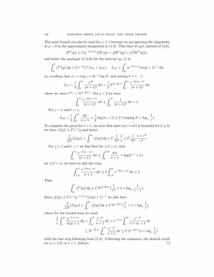
186 DONGWOO SHEEN, IAN H. SLOAN, AND VIDAR THOMEE
The same bound can also be used for α ≥ 1 because we are ignoring the singularityat y = 0 in the approximate integration in (1.9). This time we get, instead of (2.6),
|F ′′(y)| ≤ Cy−3+1/α(|W (y)|+ y|W ′(y)|+ y2|W ′′(y)|),and hence the analogue of (2.8) for the interval (y1, 1) is∫ 1
y1
|f ′′(y)| dy ≤ Cτ−3(τ2J1N + J2N ), JjN =∫ 1
y1
y−3+1/α(σ(y) + 1)−j dy,
or, recalling that σ1 = σ(y1) = 2τ−1 logN , and setting δ = τ − t,
JjN =τ
2
∫ σ1
0
eδσ
(σ + 1)jdσ =
τ
2N2−2t/τ
∫ σ1
0
e−δ(σ1−σ)
(σ + 1)jdσ,
where we used eδσ1 = N2−2t/τ . For j = 2 we have∫ σ1
0
e−δ(σ1−σ)
(σ + 1)jdσ ≤
∫ ∞
0
1(σ + 1)2
dσ = 1.
For j = 1 and t = τ ,
J1N =τ
2
∫ σ1
0
dσ
σ + 1=τ
2log(σ1 + 1) ≤ Cτ(log logN + log+
1τ).
To complete the proof for t = τ , we note that since w(γ+νσ) is bounded for σ ≥ 0,we have |f(y)| ≤ Cτ−1y and hence
12N
|f(y1)|+∫ y1
0
|f(y)| dy ≤ C1N2
1τ≤ C
1N2
1 + τ2
τ2.
For j = 1 and t < τ we find first for 1/δ ≥ σ1 that∫ σ1
0
e−δ(σ1−σ)
(σ + 1)jdσ ≤
∫ 1/δ
0
d σ
σ + 1= log(δ−1 + 1);
for 1/δ < σ1 we have to add the term∫ σ1
1/δ
e−δ(σ1−σ)
σ + 1dσ ≤ δ
∫ σ1
1/δ
e−δ(σ1−σ) dσ ≤ 1.
Thus ∫ 1
y1
|f ′′(y)| dy ≤ CN2−2t/τ (1τ2
+ 1 + log+
1τ − t
).
Since |f(y)| ≤ Cτ−1y−1+1/α(σ(y) + 1)−1 we also have
12N
|f(y1)|+∫ y1
0
|f(y)| dy ≤ CN−2t/τ (1τ
+ 1 + log+
1t),
where for the second term we used
2τ
∫ y1
0
y−1+1/α
σ(y) + 1dy =
∫ ∞
σ1
e−σt
σ + 1dσ = e−σ1t
∫ ∞
0
e−xt
x+ σ1 + 1dx
≤ N−2t/τ
∫ ∞
0
e−xt
x+ 1dx ≤ CN−2t/τ (1 + log+
1t),
with the last step following from (2.4). Collecting the estimates, the desired resultfor α > 1/2, or t < τ , follows.

TIME-DISCRETIZATION OF PARABOLIC PROBLEMS 187
We remark that if instead of U(t) we use the modified approximate solutionUε(t) introduced after the proof of Proposition 2.1, then the error bound takes thesimpler form
‖Uε(t)− u(t)‖ ≤ Ce−γt‖Aεu0‖
1N2
1 + t2
τ2, t ≥ τ,
1N2t/τ
1 + τ2
τ2, t ≤ τ.
In fact, for t ≥ τ, we have instead of (2.7)
|f ′′(y)| ≤ Cy−3+1/ατ−3(t2 + 1)(σ(y) + 1)−1−ε
and hence (cf. (2.8) and (2.9))∫ 1
0
|f ′′(y)| dy ≤ Cτ−2(t2 + 1)∫ ∞
0
e−σ(t−τ)(σ + 1)−1−ε dσ ≤ Cετ−2(t2 + 1).
The estimate for t ≤ τ is derived similarly.Let us now comment on our above choice of the slope 1 in Γ = Γγ . In fact,
choosing instead Γγ,s = z = γ + σ ± isσ; 0 ≤ σ < ∞, it is easy to see that thebounds for ‖w(j)(z)‖ have to be multiplied by (1 + 1/s)j+1. On the other hand,from the proof of Theorem 2.2 we see that the factors ν = 1 + i in front of f(y)and in W ′ and W ′′ should now be replaced by νs = 1 + is. The total change in theerror bound in Theorem 2.2 would be a factor (s+1/s)3, and we therefore see thats should be chosen neither too large nor too small. A natural choice is s = 1.
We remark that the error estimate of Theorem 2.2 holds not only for the trape-zoidal rule but also for any other composite rule on the uniform partition yj , j =0, . . . , N , which is exact for linear functions. In particular, it holds for the Simpsonrule, but with less than optimal accuracy.
Before turning to the full treatment of Simpson’s rule, we pause to exhibit somenumerical values of the quadrature errors εN = εN (t;λ) = |Q(t;λ) − e−λt|, whichillustrate the behavior of our time discretization method based on the trapezoidalrule. Table 1 shows these errors εN for τ = 1, λ = 1, and γ = 0, with N = 20, 40, 80and 160, and Table 2 the corresponding errors when τ = 1, λ = 1, γ = 0.75. HereρN = log2(εN/2/εN ) is the local convergence rate.
We observe that the predicted O(N−2) asymptotic convergence rate for t > τ = 1is very clear in the tables. For values of t smaller than τ the accuracy and the orderof convergence deteriorate, broadly in line with the predictions of Theorem 2.2, butoscillations in the error prevent a clear determination of orders of convergence. Wealso note that the errors at t ≈ τ are smaller for γ = 0 than for γ = 0.75, butthat the situation is reversed for large values of t, which is consistent with the errorbounds of Theorem 2.2.
In Table 3 we show the effect of varying τ , by repeating the calculation nowwith τ = 1
2 , γ = 0. We see, on the one hand, that the O(N−2) convergence ratenow persists, as it should, for τ > 1
2 . On the other hand the absolute errors for1 ≤ τ < 2 are larger than we observed in Table 1. Again this is broadly in line withthe predictions of the theorem, given the appearance of the τ−2 terms in the errorbounds. The results in these tables and this discussion motivate our suggestionthat the results for a fixed value of τ be used only for a limited range of t values,such as τ ≤ t ≤ 2τ for the case γ = 0.
We now turn to the case when the time discretization is accomplished by Simp-son’s rule. We first remark that the stability result of Proposition 2.1 remains valid

188 DONGWOO SHEEN, IAN H. SLOAN, AND VIDAR THOMEE
Table 1. Time discretization errors for trapezoidal rule with τ =1, λ = 1, γ = 0.
t ε20 ε40 ρ40 ε80 ρ80 ε160 ρ160
0.2 0.253E-01 0.128E-01 0.98 0.543E-02 1.24 0.130E-02 2.060.4 0.197E-02 0.173E-02 0.19 0.950E-03 0.86 0.371E-03 1.360.6 0.172E-03 0.897E-04 0.94 0.964E-04 -0.10 0.443E-04 1.120.8 0.365E-03 0.993E-04 1.88 0.154E-04 2.69 0.552E-06 4.801.0 0.150E-03 0.266E-04 2.50 0.685E-05 1.96 0.225E-05 1.601.2 0.151E-04 0.611E-05 1.30 0.195E-05 1.64 0.422E-06 2.211.4 0.806E-04 0.195E-04 2.05 0.500E-05 1.96 0.125E-05 2.001.6 0.185E-03 0.465E-04 1.99 0.116E-04 2.00 0.290E-05 2.001.8 0.292E-03 0.730E-04 2.00 0.182E-04 2.00 0.456E-05 2.002.0 0.398E-03 0.995E-04 2.00 0.249E-04 2.00 0.622E-05 2.003.0 0.929E-03 0.232E-03 2.00 0.580E-04 2.00 0.145E-04 2.004.0 0.146E-02 0.365E-03 2.00 0.912E-04 2.00 0.228E-04 2.005.0 0.199E-02 0.498E-03 2.00 0.124E-03 2.00 0.311E-04 2.006.0 0.253E-02 0.630E-03 2.00 0.158E-03 2.00 0.394E-04 2.00
Table 2. Time discretization errors for trapezoidal rule with τ =1, λ = 1, γ = 0.75.
t ε20 ε40 ρ40 ε80 ρ80 ε160 ρ160
0.2 0.282E-01 0.127E-01 1.15 0.524E-02 1.28 0.139E-02 1.920.4 0.438E-02 0.219E-03 4.32 0.327E-03 -0.58 0.185E-03 0.820.6 0.456E-02 0.123E-02 1.89 0.353E-03 1.80 0.101E-03 1.800.8 0.404E-02 0.102E-02 1.98 0.252E-03 2.03 0.611E-04 2.041.0 0.323E-02 0.811E-03 2.00 0.203E-03 2.00 0.510E-04 1.991.2 0.260E-02 0.657E-03 1.98 0.165E-03 2.00 0.411E-04 2.001.4 0.209E-02 0.529E-03 1.99 0.132E-03 2.00 0.331E-04 2.001.6 0.168E-02 0.423E-03 1.99 0.106E-03 2.00 0.265E-04 2.001.8 0.133E-02 0.337E-03 1.99 0.842E-04 2.00 0.211E-04 2.002.0 0.105E-02 0.266E-03 1.99 0.666E-04 2.00 0.166E-04 2.003.0 0.275E-03 0.698E-04 1.98 0.175E-04 2.00 0.437E-05 2.004.0 0.246E-04 0.655E-05 1.91 0.165E-05 1.99 0.412E-06 2.005.0 0.382E-04 0.938E-05 2.02 0.234E-05 2.00 0.585E-06 2.006.0 0.416E-04 0.103E-04 2.01 0.258E-05 2.00 0.645E-06 2.00
in this situation, since the points σj are still defined by (1.12) and the weightsωj(t) are now bounded by 4
3 times those in (1.13). For the error we now have thefollowing estimate.
Theorem 2.3. Let τ > 0, and assume that the eigenvalues of A are bounded belowby λ0, and that 0 ≤ γ < λ0. Assume that the quadrature approximation U(t) isobtained by applying Simpson’s rule (1.14) (with the y0 term omitted) to the integral(1.5), where g(t;σ) is defined by (1.6) and α is chosen so that αt = τ/4. Then there

TIME-DISCRETIZATION OF PARABOLIC PROBLEMS 189
Table 3. Time discretization errors for trapezoidal rule with τ =1/2, λ = 1, γ = 0.
t ε20 ε40 ρ40 ε80 ρ80 ε160 ρ160
0.2 0.301E-03 0.129E-02 -2.09 0.838E-03 0.62 0.347E-03 1.270.4 0.166E-02 0.424E-03 1.97 0.969E-04 2.13 0.210E-04 2.210.6 0.110E-02 0.278E-03 1.99 0.699E-04 1.99 0.174E-04 2.010.8 0.689E-03 0.172E-03 2.00 0.431E-04 2.00 0.108E-04 2.001.0 0.263E-03 0.662E-04 1.99 0.166E-04 2.00 0.414E-05 2.001.2 0.161E-03 0.399E-04 2.01 0.996E-05 2.00 0.249E-05 2.001.4 0.585E-03 0.146E-03 2.00 0.365E-04 2.00 0.912E-05 2.001.6 0.101E-02 0.252E-03 2.00 0.630E-04 2.00 0.158E-04 2.001.8 0.143E-02 0.358E-03 2.00 0.895E-04 2.00 0.224E-04 2.002.0 0.186E-02 0.464E-03 2.00 0.116E-03 2.00 0.290E-04 2.00
exists C = C(λ0 − γ) > 0, such that
‖U(t)− u(t)‖ ≤ C‖u0‖e−γt
1N4
( 1 + t4
τ4(1 + t− τ)+t4
τ4log+
1t− τ
), t > τ,
1N4
(log logN +
1τ4
+ log+
1τ
), N ≥ 3, t = τ,
1N4t/τ
(1 + τ4
τ4+ log+
1τ − t
+ log+
1t
), 0 < t < τ.
Proof. With f(u) and F (u) as earlier, we have this time
ε(t;λ) ≤ Ce−γt
N4
∫ 1
0
|f (iv)(y)| dy.
For t > τ , or α < 1/4, (2.6) is replaced by
|F (iv)(y)| ≤ Cy−5+1/α4∑
j=0
αj−4yj |W (j)(y)|.
Here
yj|W (j)(y)| ≤ C∑l≤j
τ−l|w(l)(γ + νσ(y))| ≤ C∑l≤j
τ−l(σ(y) + 1)−l−1, for j ≤ 4,
so that
|F (iv)(y)| ≤ Cy−5+1/ατ−4(t4(σ(y) + 1)−1 + (σ(y) + 1)−2).
We conclude that, with
Jj =∫ 1
0
y−5+1/α(σ(y) + 1)−j dy, j = 1, 2,
we have ∫ 1
0
|f (iv)(y)| dy ≤ Cτ−5(t4J1 + J2),
and the argument is completed as before.

190 DONGWOO SHEEN, IAN H. SLOAN, AND VIDAR THOMEE
Table 4. Time discretization errors for Simpson’s rule with τ =1, λ = 1, γ = 0.
t ε20 ε40 ρ40 ε80 ρ80 ε160 ρ160
0.2 0.278E-02 0.161E-02 0.78 0.688E-03 1.23 0.183E-03 1.910.4 0.233E-03 0.131E-04 4.15 0.120E-04 0.13 0.436E-05 1.450.6 0.983E-05 0.334E-05 1.56 0.619E-06 2.43 0.822E-07 2.910.8 0.330E-04 0.390E-07 9.73 0.481E-07 -0.30 0.566E-08 3.091.0 0.222E-04 0.469E-06 5.56 0.329E-07 3.83 0.226E-08 3.871.2 0.208E-04 0.389E-06 5.74 0.341E-07 3.51 0.204E-08 4.061.4 0.184E-04 0.438E-06 5.40 0.344E-07 3.67 0.211E-08 4.031.6 0.176E-04 0.511E-06 5.11 0.379E-07 3.76 0.233E-08 4.021.8 0.177E-04 0.626E-06 4.83 0.440E-07 3.83 0.271E-08 4.022.0 0.187E-04 0.779E-06 4.59 0.527E-07 3.89 0.327E-08 4.01
For t ≤ τ , corresponding to α ≥ 14 , we use instead of (1.15) the estimate
|SNf − If | ≤ C
N4
∫ 1
y2
|f (iv)(y)| dy +4
3N|f(y1)|+ 1
3N|f(y2)|+
∫ 2N
0
|f(y)| dy,
which is the appropriate bound for Simpson’s rule for the interval [y2, 1], togetherwith estimation by zero in the interval [0, y2]. The remainder of the proof followsin the same manner as in Theorem 2.2.
We complete this section by presenting in Table 4 the analogue for Simpson’srule of Table 1. Thus Table 4 shows the quadrature error εN = |Qτ (t;λ)−e−λt| forτ = 1, λ = 1, and γ = 0, with N = 20, 40, 80, and 160, for Simpson’s rule. For t > τthe predicted O(N−4) accuracy is clearly seen, and the errors are correspondinglysmall, while for t < τ the reduced rate of convergence is particularly clear.
It should be emphasized that in the present method Simpson’s rule with a givenvalue of N requires exactly the same computational effort as the trapezoidal rule.A comparison between Tables 1 and 4 will convince the reader that Simpson’srule is superior. The numerical results in Table 4 also suggest that in practicalcalculations, such as the finite-element calculations of the next section, a value of,say, N = 40 in Simpson’s rule should be more than adequate in most cases.
3. Application to the finite element method
We now consider the application of our quadrature based methods to the “par-abolic” equation in the piecewise linear space Vh which has been obtained bydiscretization in the space of the initial-boundary value problem (1.16), i.e., thesemidiscrete problem (1.18). With our earlier definitions, this may be written
uh,t +Ahuh = 0, for t > 0, with uh(0) = Phu0.
As explained in the introduction, our fully discrete approximation Uh(t) ∈ Vh isthen obtained by the application of one of our quadrature methods to the integral(1.5), where now g(t;σ) in (1.6) is replaced by gh(t;σ), defined in terms of thefinite element approximation wh(z) from (1.17) of the solution w(z) of the elliptic

TIME-DISCRETIZATION OF PARABOLIC PROBLEMS 191
equation in (1.4), so that
Uh(t) = Q(t;Ah)Phu0 =N∑
j=1
ωj(t)gh(t;σj), gh(t;σ) =1π
Im(νe−iσtwh(γ + νσ)
).
The error Uh − u may be handled by splitting it as
Uh(t)− u(t) = (Uh(t)− uh(t)) + (uh(t)− u(t)).(3.1)
If the trapezoidal rule is used for the time discretization, then we may apply The-orem 2.2 to the first part of the error, because the smallest eigenvalue λh,1 of Ah isbounded below by the smallest eigenvalue λ1 of A. Hence, since ‖Phu0‖ ≤ ‖u0‖, thefirst part of the error in (3.1) is bounded in norm by the error bound in Theorem2.2. The second part of the error in (3.1) is bounded by (cf. [10])
‖uh(t)− u(t)‖ ≤ Ch2t−1e−γt‖u0‖, for t > 0,
or, more generally, also for smoother initial data, by
‖uh(t)− u(t)‖ ≤ Ch2t−1+εe−γt‖Aεu0‖, for t > 0, 0 ≤ ε ≤ 1;
together these estimates yield complete error estimates for our method. We remarkthat for smooth initial data the error in the spatially semidiscrete equation is thusO(h2), uniformly down to t = 0, but that the O(N−2) error bound in the quadraturemethod based on the trapezoidal rule holds only for t > τ , even when initial dataare smooth.
Similarly, for the case of Simpson’s rule the error bound for ‖Uh(t) − uh(t)‖ isexactly as in Theorem 2.3, and the total error for t > τ is O(N−4 + h2).
We now give some illustrations, beginning with the spatially one-dimensionalproblem
ut = uxx, in [0, π], with u(0, t) = u(π, t) = 0, for t > 0,
u(x, 0) = u0(x), in [0, π].(3.2)
In Tables 5, 6, and 7 we exhibit errors εN,M in the numerical results for the initialfunction u0(x) = (5π/2)−1/2(sinx + 2 sin 2x) (with ‖u0‖ = 1) for, respectively, thetrapezoidal rule, Simpson’s rule, and, for comparison, the Crank-Nicolson method.In all cases the spatial discretization uses piecewise linear approximations on regularmeshes, with h = π/M, and N is chosen as 20, 40, 80, and 160 for both the trape-zoidal rule and the Crank-Nicolson method (with time step 1/N), and as 10, 20, and40 for Simpson’s rule. In Tables 5 and 6 we choose τ = 1 and γ = 0, and show resultsonly for τ ≤ t ≤ 2τ , which is the recommended way of using the method, and for theCrank-Nicolson method we restrict ourselves to t = 1 and t = 2. In Tables 5 and 7,ρN,M = log2(εN/2,M/2/εN,M), and in Table 6, ρN,M = log2(εN/2,M/4/εN,M). Theresults again show the expected O(N−2+h2) = O(N−2+M−2) order of convergencefor the trapezoidal and Crank-Nicolson cases and O(N−4 + h2) = O(N−4 +M−2))for Simpson’s rule. Note that the higher order of the discretization in Simpson’srule compared with the Crank-Nicolson method allows us to obtain accuracy oforder 10−6 in the interval [1, 2] with a much coarser time discretization.
As our next illustration, we consider again the spatially one-dimensional problem(3.2), now with the nonsmooth initial function u0(x) = (π/2)−1/2 for π
4 ≤ x ≤ 3π4 ,
and u0(x) = 0 for other x in [0, π] (again with ‖u0‖ = 1). The analogues of Tables5, 6, and 7 above are exhibited in Tables 8, 9, and 10. Since the Crank-Nicolsonmethod is known not to deal well with nonsmooth data, we exhibit also the result

192 DONGWOO SHEEN, IAN H. SLOAN, AND VIDAR THOMEE
Table 5. Trapezoidal rule errors for 1D heat equation with τ =1, γ = 0.
t ε20,50 ε40,100 ρ40,100 ε80,200 ρ80,200 ε160,400 ρ160,400
1.0 0.129E-03 0.262E-04 2.29 0.667E-05 1.98 0.201E-05 1.731.2 0.796E-04 0.192E-04 2.05 0.481E-05 1.99 0.121E-05 1.991.4 0.849E-04 0.210E-04 2.02 0.537E-05 1.97 0.134E-05 2.001.6 0.123E-03 0.311E-04 1.98 0.775E-05 2.00 0.194E-05 2.001.8 0.172E-03 0.430E-04 2.00 0.107E-04 2.00 0.268E-05 2.002.0 0.223E-03 0.557E-04 2.00 0.139E-04 2.00 0.348E-05 2.00
Table 6. Simpson’s rule errors for 1D heat equation with τ =1, γ = 0.
t ε10,25 ε20,100 ρ20,100 ε40,400 ρ40,400
1.0 0.216E-02 0.320E-04 6.08 0.184E-05 4.121.2 0.173E-02 0.265E-04 6.02 0.131E-05 4.341.4 0.136E-02 0.226E-04 5.91 0.113E-05 4.321.6 0.107E-02 0.208E-04 5.69 0.105E-05 4.301.8 0.836E-03 0.197E-04 5.41 0.103E-05 4.262.0 0.643E-03 0.192E-04 5.07 0.103E-05 4.21
Table 7. Crank-Nicolson errors for 1D heat equation.
t ε20,50 ε40,100 ρ40,100 ε80,200 ρ80,200 ε160,400 ρ160,400
1.0 0.975E-03 0.245E-03 2.00 0.612E-04 2.00 0.153E-04 2.002.0 0.145E-03 0.363E-04 2.00 0.908E-05 2.00 0.227E-05 2.00
Table 8. As in Table 5 with nonsmooth initial data.
t ε20,50 ε40,100 ρ40,100 ε80,200 ρ80,200 ε160,400 ρ160,400
1.0 0.139E-03 0.298E-04 2.22 0.754E-05 1.99 0.215E-05 1.811.2 0.709E-04 0.191E-04 1.89 0.499E-05 1.94 0.122E-05 2.041.4 0.261E-04 0.697E-05 1.90 0.171E-05 2.03 0.427E-06 2.001.6 0.454E-04 0.113E-04 2.01 0.281E-05 2.00 0.701E-06 2.001.8 0.101E-03 0.251E-04 2.01 0.627E-05 2.00 0.157E-05 2.002.0 0.159E-03 0.395E-04 2.01 0.988E-05 2.00 0.247E-05 2.00
obtained by the modification of using the backward Euler method for the first twotime steps, which smooths the initial data (cf. [10]). As expected, the results inTables 8 and 9 show the same behavior for nonsmooth as for smooth initial data.For the nonsmooth initial data the Simpson’s rule results in Table 9 with N = 40compare very favorably with even the modified Crank-Nicolson results with 160time steps.

TIME-DISCRETIZATION OF PARABOLIC PROBLEMS 193
Table 9. As in Table 6 with nonsmooth initial data.
t ε10,25 ε20,100 ρ20,100 ε40,400 ρ40,400
1.0 0.204E-02 0.274E-04 6.22 0.127E-05 4.431.2 0.164E-02 0.262E-04 5.97 0.119E-05 4.461.4 0.129E-02 0.242E-04 5.74 0.116E-05 4.381.6 0.100E-02 0.227E-04 5.47 0.113E-05 4.331.8 0.776E-03 0.216E-04 5.16 0.111E-05 4.282.0 0.586E-03 0.209E-04 4.81 0.111E-05 4.23
Table 10. Crank-Nicolson 1D errors, without and with backwardEuler smoothing.
t ε20,50 ε40,100 ρ40,100 ε80,200 ρ80,200 ε160,400 ρ160,400
1.0 0.504E-01 0.263E-01 0.94 0.186E-01 0.50 0.132E-01 0.502.0 0.367E-01 0.168E-01 1.12 0.119E-01 0.50 0.843E-02 0.501.0 0.158E-02 0.402E-03 1.97 0.102E-03 1.98 0.256E-04 1.992.0 0.499E-03 0.128E-03 1.96 0.325E-04 1.98 0.818E-05 1.99
Table 11. Simpson’s rule errors for 2D heat equation, with τ =1, γ = 0.
t ε16,25 ε32,100 ρ32,100
1.0 0.335E-03 0.209E-04 4.001.2 0.269E-03 0.166E-04 4.021.4 0.212E-03 0.131E-04 4.021.6 0.165E-03 0.102E-04 4.021.8 0.129E-03 0.804E-05 4.002.0 0.103E-03 0.644E-05 4.00
Finally, we consider the spatially two-dimensional problem version of the bound-ary value problem for the heat equation, with Ω = [0, π]× [0, π],
ut = ∆u, in Ω, u(x, y, t) = 0, for (x, y) ∈ ∂Ω, t > 0,
u(x, y, 0) = u0(x, y), in Ω,
with (non-smooth) initial data u0(x, y) = χ[ π5 , 4π
5 ]×[ π5 , 4π
5 ](x, y). The finite elementspace for the spatial approximation is obtained by dividing Ω into M ×M identicalrectangles (h = π/M), and using piecewise bilinear elements on this mesh. For thetime discretization we adopt Simpson’s rule and choose τ and γ to have the values1 and 0, respectively.
In Table 11 we present the resulting L2(Ω) errors for N = 32 and M = 100, andalso (to allow us to check the predicted O(h2 +N−4) rate of convergence) N = 16and M = 25. Evidently the rate of convergence and the absolute errors in the timeinterval [τ, 2τ ] are both highly acceptable.
To give substance to the claim that this is a parallel method, the results in Table11 were obtained (using the Yale Sparse Matrix Package [4], an efficient version ofGaussian elimination, with double complex arithmetic) on a 16-processor IBM SP2,

194 DONGWOO SHEEN, IAN H. SLOAN, AND VIDAR THOMEE
Table 12. Computing time and speedup ratio for 2D heat equation.
Problem Size P 1 2 4 8 16N = 32 T 81.3 40.5 20.7 10.6 5.6M = 50 ρ 2.00 1.95 1.95 1.89N = 32 T 942 471 236 119 61M = 100 ρ 2.00 2.00 1.98 1.94
whose main architectural feature is that it has 16 essentially identical processors,with no shared memory. The main part of the computation is of course the solutionof the elliptic finite-element problem (1.17), for z = zj = γ + νσj , j = 1, . . . , N .The N such problems were first solved one after another on a single processor; thenfor comparison distributed between 2 processors, so that each processor had to solveonly half the number of elliptic problems; then distributed over 4 processors, andso on. The total computer clock times (including overheads) required with 1, 2, 4,8, and 16 processors are reported in Table 12 for N = 32 and M = 100, as wellas M = 50 for comparison. In Table 12 the labels P, T , and ρ denote the num-ber of processors, the total computer clock time in seconds, and the speedup ratioT (P/2)/T (P ), respectively. When the size of the finite element problem changesfrom M = 50 to 100 the speedup ratios become closer to two, reflecting the tru-ism that the bigger the size of the distributed problems, the more effective theparallelization. Since the total time for the largest problem continues to decreaseroughly in proportion to the number of processors for P up to 16, the paralleliza-tion has been successful, and indeed could profitably employ many more processorsthan the 16 currently available to us. A parallel implementation with more than16 processors would be expected to be even more beneficial for parabolic problemsin three space dimensions.
References
1. P. J. Davis and P. Rabinowitz, Methods of Numerical Integration, Academic Press, New York,1975. MR 56:7119
2. J. Douglas, Jr., J. E. Santos, D. Sheen, and L. S. Bennethum, Frequency domain treatment ofone-dimensional scalar waves, Math. Mod. Meth. Appl. Sci. 3 (1993), 171-194. MR 94g:65111
3. J. Douglas, Jr., J. E. Santos, and D. Sheen, Approximation of scalar waves in the space-frequency domain, Math. Mod. Meth. Appl. Sci 4 (1994), 509-531. MR 95e:65089
4. S. C. Eisenstat, Jr., H. E. Elman, N. H. Schultz, and A. H. Sherman, The (new) Yale SparseMatrix Package, Elliptic Problem Solvers II (A. L. Schoenstadt and G. Birkhoff, eds.), Aca-demic Press, New York, 1983, pp. 45–52. MR 85g:65007
5. E. Gallopoulos and Y. Saad, Efficient solution of parabolic equations by Krylov approximationmethods, SIAM J. Sci. Statist. Comput. 13 (1992), 1236–1264. MR 93d:65085
6. M. Hochbruck and C. Lubich, On Krylov Subspace Approximations to the Matrix ExponentialOperator, SIAM J. Numer. Anal. 34 (1997), 1911-1925. MR 98h:65018
7. C.-O. Lee, J. Lee, and D. Sheen, A frequency-domain method for finite element solutions ofparabolic problems, RIM-GARC Preprint 97–41, Department of Mathematics, Seoul NationalUniversity, 1997.
8. A. Pazy, Semigroups of Linear Operators and Applications to Partial Differential Equations,
Springer-Verlag, New York, 1983. MR 85g:470619. D. Sheen and Y. Yeom, A frequency-domain parallel method for the numerical approxima-
tion of parabolic problems, RIM-GARC Preprint 96–38, Department of Mathematics, SeoulNational University, 1996.

TIME-DISCRETIZATION OF PARABOLIC PROBLEMS 195
10. V. Thomee, Galerkin Finite Element Methods for Parabolic Problems, Springer Series inComputational Mathematics, Vol. 25, Springer-Verlag, Berlin Heidelberg New York, 1997.MR 98m:65007
11. R. S. Varga, Functional Analysis and Approximation Theory in Numerical Analysis, Confer-ence Board of the Mathematical Sciences Regional Conferences Series in Applied Mathematics,No. 3, SIAM, Philadelphia, PA, 1971. MR 46:9602
Department of Mathematics, Seoul National University, Seoul 151-742, Korea
E-mail address: [email protected]
School of Mathematics, University of New South Wales, Sydney 2052, Australia
E-mail address: [email protected]
Department of Mathematics, Chalmers University of Technology, S-412 96 Gote-
borg, Sweden
E-mail address: [email protected]