A parallel finite element program on a Beowulf cluster

V.E. Sonzogni*, A.M. Yommi, N.M. Nigro, M.A. Storti

International Center for Computer Methods in Engineering (CIMEC), INTEC—Universidad Nacional del Litoral—CONICET, Guemes 3450,

3000 Santa Fe, Argentina

Received 14 November 2000; accepted 1 July 2002

Abstract

Some experiences on writing a parallel finite element code on a Beowulf cluster are shown. This cluster is made up of seven Pentium III

processors connected by Fast Ethernet. The code was written in Cþþ making use of MPI as message passing library and parallel extensible toolkit

for scientific computations. The code presented here is a general framework where specific applications may be written. In particular CFD

applications regarding Laplace equations, Navier–Stokes and shallow water flows have been implemented. The parallel performance of this

application code is assessed and several numerical results are presented. q 2002 Civil-Comp Ltd and Elsevier Science Ltd. All rights reserved.

Keywords: Beowulf clusters; Parallel computing; Finite element method; Computational fluid dynamics; Distributed computations; Computational mechanics

1. Introduction

CIMEC is an academic research center where numerical

methods are applied to some engineering problems in areas

such as CFD, solid materials modeling, dynamics of

mechanisms and structures, metal casting, forming pro-

cesses and biomechanics. Computational requirements for

some problems exceed the capabilities of the available

equipment (workstations). Attempts to improve our com-

puter power led us to exploit distributed computation on

network of workstations (NOWs) and latter on a Beowulf

cluster.

In the history of computers there was a time when the

computer power was in the hands of some supercomputers,

of sophisticated technology and very high prices. The need

for growing performances led to parallel computing. On the

other hand, the increase in microprocessors technology

made the gap between these and supercomputers to become

shorter and shorter. The performance/price ratio attracted

attention to the use of microprocessors on a parallel

environment. In 1994 a machine composed of micropro-

cessors connected by channel bonded Ethernet, gave place

to the so-called Beowulf class cluster computers [1].

The Beowulf clusters share some characteristics; the

hardware is constructed by the users themselves making use

of commodity of the shelf (COTS) components. Usually

microprocessors (Intel Pentium II, P6) of ease availability

are connected through Fast Ethernet and Fast Ethernet

switches. The operating system adopted has been Linux,

which is widely available; GNU compilers have also been

used [2]. Software tools for message passing such as PVM

[3] or MPI [4] are also part of the Beowulf clusters.

There exists a world wide Beowulf community (like the

Linux community) which is composed of independent

researchers and developers, who share their experiences.

This is a very attractive proposal for our university, which

has had usually limited resources. In this context, we began

the construction of a cluster, which then had 7 nodes, and is

continuously growing and we expect it to reach 20 nodes

very soon. These are Pentium III, diskless processors

connected by Fast Ethernet. One of them has a server

disk. We have MPI and PVM as message passing libraries.

In this work we present some results regarding the

implementation of a general purpose, multi-physics, FEM

code oriented toward CFD applications running on Beowulf

clusters and based on the MPI message passing library. We

have also used the parallel extensible toolkit for scientific

computations (PETSc). This one provides an environment

for distributed programming allowing different levels of

compromise to the programmer with parallelism. One may

let PETSc perform the entire parallel tasks (allocation of

data, solving systems, etc.) or may program explicitly the

parallel tasks.

We have developed FEM programs to study: Laplace,

0965-9978/02/$ - see front matter q 2002 Civil-Comp Ltd and Elsevier Science Ltd. All rights reserved.

PII: S0 96 5 -9 97 8 (0 2) 00 0 59 -5

Advances in Engineering Software 33 (2002) 427–443

www.elsevier.com/locate/advengsoft

* Corresponding author. Tel.: þ54-342-4559175; fax: þ54-342-4550944.

E-mail address: sonzogni@intec.unl.edu.ar (V.E. Sonzogni).

shallow water and incompressible Navier – Stokes

equations. The incompressible Navier–Stokes equations

are solved by two different numerical approaches, one is the

so-called ‘fractional-step’ strategy and other is that

introduced by Tezduyar called SUPG–PSPG. One of the

strongest restrictions for solving such a system comes from

the incompressibility condition that inhibits the use of

explicit integration algorithms, which are more common for

compressible flows and shallow water. In this sense the

fractional step and related algorithms treat to decouple this

system in a certain number of linearized and scalar substeps.

In the first step, called predictor, the pressure gradient is

treated explicitly giving rise to a set of three advection

diffusion equations for the three components of the velocity,

which is stabilized with the well-known SUPG method. The

linear system corresponding to this substep is a typical mass

matrix plus diffusion term, and may or may not include an

advection term depending on whether the advection term is

treated explicitly or implicitly. However, even in the case of

not including an advection term, the system is non-

symmetric due to the SUPG ‘biased’ weighing. In the

following substep a Poisson equation is solved for the

pressure–time increment and, finally, in the third step a

projection (mass matrix) system is solved. The last two

substeps have symmetric positive definite matrices. Even

though the computational cost is drastically reduced

unfortunately the solution is highly dependent on the time

step being critical in its selection. On the other hand the

SUPG–PSPG strategy is a formulation based on an equal

order interpolation of velocity and pressure variables that

circumvents the Brezzi–Babuska condition by the addition

of two perturbation functions to the standard Galerkin

formulation. In this way it is feasible to avoid not only the

checkerboard modes but also the typical oscillations in

advection dominated problems. In both the approaches the

choice of the solver for each time step is linked to the

parallelism strategy.

The aim of this work was to conduct some experiments

with parallel implementations of a finite element code on

our Beowulf cluster, focusing on the task of solving the

linear equations systems. Several linear equations solvers

have been tested. They include calls to PETSc tools or to

some solvers that were developed specifically for this

program. The program has been written in Cþþ . Topics

like scalability and load balancing have been considered.

2. Beowulf cluster

Parallel computing was traditionally a matter of very

expensive hardware and software. In the late 1980s it was

very common to use cluster of workstations (COWs). This

allowed people at universities to run jobs in parallel in a

NOWs at night, when the user load is low. In most cases the

workstations ran some kind of Unix OS, and most of the

message passing libraries (PVM, MPI) were developed

oriented toward the Unix world.

With the massive arrival of PCs many people attempted

to use them for parallel applications. Today Intel processors

have the best processing speed/cost ratio. But in order to use

the software developed for scientific computations, a

version of Unix for PCs was needed. In 1991, the

GNU/Linux OS was born. Nowadays, an array of Intel

processors running Linux is perhaps the cheapest way to

access the parallel computing world with the best speed/-

performance ratio (arrays of DEC/Alphas running Linux are

also a popular choice). From Ref. [6] a ‘Beowulf cluster’ is

“A cluster of mass-market commodity off-the-shelf

(M2COTS) PCs interconnected by low cost LAN technol-

ogy running an open source code Unix-like OS and

executing parallel applications programmed with and

industry standard message passing model and library.”

The ‘Beowulf Project’ was originally developed at the

Goddard Space Flight Center (GSFC).

Numerical experiments have been performed with a

cluster built with seven Intel Pentium III processors, with

128 MB RAM each, (256 MB for the server) linked through

a switched Fast Ethernet network (100 Mbit/s, latency ¼

Oð100Þ) supported by a 3COM SuperStack 3300 switch in

full duplex mode. The configuration of the cluster is ‘disk-

less’, i.e. the nodes do not have a hard disk. At start, they

boot from a floppy diskette, loading the Linux RedHat 5.2

kernel (kernel version 2.0.36) and then, they send a RARP

request to the server, who answers telling them their IP

(according to their MAC addresses) and their root directory

(actually a subdirectory of /tftpboot in the server).

Then, the nodes mount via NFS their root directories on the

server and proceed to the rest of the boot sequence. Some of

the performance issues related to the disk-less configuration

are the following ones:

† It represents a saving because the nodes do not need a

hard disk.

† The cluster is easier to manage, since a change in

configuration is performed locally on the node root

directories, (subdirectories of /tftpboot on the

server) and the kernel on the floppies. For instance, a

new node can be easily added to the cluster by inserting a

copy of the boot floppy and running a script, which takes

charge of creating the root directory in /tftpboot for

the new node.

† Nodes do not have swap memory. This could be

considered a drawback but, swap memory degrades

performance so much that it is useless, and moreover,

memory for Intel based clusters is so cheap that

calculations are in most cases CPU bound. Anyway, if

some amount of swap memory is desired, it is better to

have a local (i.e. per-node) hard disk only for swap and

some local data files, and leave the root directory,

software and user accounts on a global (i.e. on the server)

partition.

V.E. Sonzogni et al. / Advances in Engineering Software 33 (2002) 427–443428

† When starting a program (with mpirun), the nodes

access the server through the network and read the entire

code to the node RAM. This can lead to a bottleneck for

very large systems but, for the codes we are running, this

delay is usually negligible with respect to the average

execution time.

3. PETSc-FEM: a general finite element code

3.1. The PETSc-FEM library

PETSc-FEM is not a FEM code but a layer of routines

that enables an ‘application writer’ to develop a typical

finite element application code to be used by the ‘end user’

[7]. However, specific application codes for Navier–Stokes,

Euler, shallow water, Laplace and advection diffusion have

been developed and included in the distribution in order to

be used by end users or, as well, to serve as a basis to

application writers for the development of other codes. This

involves usually two complimentary parts:

† The routine that describes the main algorithm (i.e. linear/

non-linear strategy, steady/unsteady, etc.), where the

application writer calls a set of routines that read the

mesh, assembles PETSc vectors and matrices, check

convergence, etc.

† The element routines compute for each element that how

a specific term (residual, stiffness matrix, etc.) is

computed.

Solution of the resulting system of equations is done by

appropriated calls to the PETSc. Typically, element routines

receive a list of elements, and should return a list of residual

vectors, matrix elements or anything else per element. These

are afterwards assembled in the global vector or matrix by

the PETSc-FEM layer. Meshes are partitioned by using

METIS, and once this is done, PETSc-FEM takes charge of

passing the appropriate elements to each processor.

Eventually, this list of elements may be internally splitted

in ‘chunks’. At the element level, calculations may (but it is

not required) be done with the help of the Newmat Cþþ

matrix library. Newmat is very interesting since it gives an

environment similar to Matlab, but may be inefficient for

small matrices computations.

PETSc-FEM is written with an Object Oriented Pro-

gramming (OOP) philosophy, but keeping in mind the target

of efficiency. The basic building object is an ‘elemset’, i.e. a

list of elements that are similar (same number of nodes,

same model, same properties). In this way, very large

elemsets can be processed efficiently, since the application

writer can perform outside the loop over the elements a

certain amount of common tasks, as decoding the element

properties, flags, etc.

Element properties are passed via general hash tables

(string ! string), so that it is very easy to add new

properties to a given element type.

3.2. The PETSc-FEM application codes

As it was mentioned in Section 3.1, the users who want to

write an application code, should provide the main

algorithm and the element routine. We will refer in this

paper to two codes: Navier–Stokes and Laplace. Problem

data are given in a file: the dimension of the problem, the

degrees of freedom per node, coordinates, type of elements,

physical properties, connectivity tables and boundary

conditions.

Data input and partition of the mesh, called Read Mesh

stage, is carried out at the same time by all processors; so,

the elapsed time in this stage will be the same in one or p

processors. This redundancy could be avoided, using the

software PAR-METIS to do the mesh partition in parallel.

In order to reduce the load unbalance, partition of the

mesh could be carried out by assigning to each processor a

load proportional to their relative speed.

Next, each processor compute the number of non-null

values of their own rows of the matrix and allocate the

memory needed. This is the stage we call Matrix Structure.

Then, an SLES context set the iterative method to be

applied, the type of preconditioning and other options such

as tolerances and parameters.

Later, in the stage Assemble Matrix, the elementary

matrices are computed and assembled. In the same way,

computation of the residual has been identified as the stage

Assemble Residual.

In the Navier–Stokes code, the stage Matrix Structure is

carried out once, keeping the sparse profile of the matrix. At

each time step, only one loop of Newton method is carried

out. Linear equations system is solved at each non-linear

iteration, using the GMRES iterative method with restart

equal 50 and with Jacobi preconditioning.

In the Laplace code, there is only one loop, and the

system of equations is solved with the Conjugate Gradient

method and with Jacobi preconditioning.

In both the programs, the solution stage was named

System Solution. In all the stages that were defined, a high

degree of parallelism is observed, except in the solution

stage, where the processors need to exchange more

information.

4. Formulation of the Navier–Stokes code

Viscous flow is well represented by Navier–Stokes

equations. The incompressible version of this model

includes the mass and momentum balances that can be

written in the following form

7·u ¼ 0 in V £ ð0; TÞ ð1Þ

V.E. Sonzogni et al. / Advances in Engineering Software 33 (2002) 427–443 429

r›u

›tþ u·7u

� �2 7·s ¼ 0 in V £ ð0; TÞ; ð2Þ

with r and u the density and velocity of the fluid and s the

stress tensor, given by

s ¼ 2pI þ 2m1ðuÞ ð3Þ

1ðuÞ ¼ 12ð7u þ ð7uÞtÞ ð4Þ

where p and m are pressure and dynamic viscosity, I

represents the identity matrix and the deformation tensor.

The initial and boundary conditions are

G ¼ Gg < Gh ð5Þ

Gg > Gh ¼ Y ð6Þ

u ¼ g on Gg ð7Þ

n·s ¼ h on Gh ð8Þ

4.1. Discretization

The spatial discretization adopted is equal order for

pressure and velocity and is stabilized through the addition

of two operators. Advection at high Reynolds numbers is

stabilized with the well-known SUPG operator, while the

PSPG operator proposed by Tezduyar et al. [5] stabilizes

the incompressibility condition, which is responsible for the

checkerboard pressure modes.

The computational domain V is divided into nel finite

elements Ve; e ¼ 1;…; nel; and let E be the set of these

elements, and H1h the finite dimensional space defined by

H1h ¼ {fhlfh [ C0ð �VÞ;fhlVe [ P1;;Ve [ E}; ð9Þ

with P1 representing polynomials of first order. The

functional spaces for weight and interpolation are defined as

Shu ¼ {uhluh [ ðH1hÞnsd ; uh

_¼ gh on Gg} ð10Þ

Vhu ¼ {whlwh [ ðH1hÞnsd ;wh

_¼ 0 on Gg} ð11Þ

Shp ¼ {qlq [ H1h} ð12Þ

where nsd is the number of spatial dimensions. The SUPG–

PSPG is written as follows: find uh [ Shu and ph [ Sh

p such

that

ðV

wh·r›uh

›tþ uh·7uh

!þðV1ðwhÞ

: sh dVþXnel

e¼1

ðVdh· r

›uh

›tþ uh·7uh

!2 7·sh

" #|fflfflfflfflfflfflfflfflfflfflfflfflfflfflfflfflffl{zfflfflfflfflfflfflfflfflfflfflfflfflfflfflfflfflffl}

ðSUPG termÞ

þXnel

e¼1

ðVeh· r

›uh

›tþ uh·7uh

!2 7·sh

" #|fflfflfflfflfflfflfflfflfflfflfflfflfflfflfflfflffl{zfflfflfflfflfflfflfflfflfflfflfflfflfflfflfflfflffl}

ðPSPG termÞ

þðV

� qh7·uh dV

¼ðGh

wh·hh dG

;wh [ Vhu ; ;qh [ Vh

p

ð13Þ

The stabilization parameters are defined as

dh ¼ tSUPGðuh·7Þwh

; ð14Þ

1h ¼ tPSPG

1

r7qh

; ð15Þ

tSUPG ¼h

2kuhkzðReuÞ ð16Þ

tPSPG ¼h#

2kUglobkzðRe#

UÞ ð17Þ

Here, Reu and ReU are Reynolds numbers based on element

properties, namely

Reu ¼kuhkh

2nð18Þ

ReU ¼kUglobkh#

2nð19Þ

where Uglob is a global characteristic velocity.

The element size h is computed with the expression

h ¼ 2Xnen

a¼1

ls·7wal !

21

ð20Þ

where wa are the functions associated to node a; nen is the

number of nodes connected to the element and s is

streamline oriented unit vector. The length h# is defined as

the diameter of a circle (sphere in 3D) equivalent to the

element area. Function zðReÞ used in Eq. (16) is defined as

zðReÞ ¼Re=3; 0 # Re , 3

1; 3 # Re

(ð21Þ

Spatial discretization leads to the following equation system

ðM þ MdÞa þ NðvÞ þ NdðvÞ þ ðK þ KdÞv

2 ðG 2 GdÞp ¼ F þ Fd ð22Þ

V.E. Sonzogni et al. / Advances in Engineering Software 33 (2002) 427–443430

Gtv þ M1a þ N1ðvÞ þ K1v þ G1p ¼ E þ E1 ð23Þ

where

v ¼ Array{uh} ð24Þ

a ¼ _v ð25Þ

p ¼ Array{ph} ð26Þ

are the vectors of velocities, accelerations and pressures,

whereas the matrices are

M ¼ðV

whrwh dV ð27Þ

Md ¼ðVdhrwh dV ð28Þ

M1 ¼ðV1hrwh dV ð29Þ

K ¼ðV

12ð7wh þ 7ðwhÞtÞ : mð7wh þ 7ðwhÞtÞdV ð30Þ

Kd ¼ 2ðVdh·7·ð2m1ðwhÞÞdV ð31Þ

K1 ¼ 2ðV1h·7·ð2m1ðwhÞÞdV ð32Þ

G ¼ðV

qh7·wh dV ð33Þ

Gd ¼ðVdh·7qh dV ð34Þ

Ge ¼ðV1h·7qh dV ð35Þ

›

›vNðvÞ ¼

ðV

wh·ruh·7wh dV ð36Þ

›

›vNdðvÞ ¼

ðVdh·ruh·7wh dV ð37Þ

›

›vNe ðvÞ ¼

ðV

h·ruh·7wh dV ð38Þ

Vector F arises from the imposition of Dirichlet and

Neumann boundary conditions, whereas vector E arises

form the Dirichlet conditions only.

5. Assessment of the parallel performance

Performance analysis of PETSc-FEM was based on the

study of some tests for Laplace and Navier–Stokes

programs.

The aim of the performance analysis was to get tools for

predicting and estimating how the PETSc-FEM codes

would behave while increasing the number of processors.

Therefore, elapsed, CPU and communication times have

been measured; speedup and efficiency have been com-

puted; and features of parallel processing, like the reduction

in processing time for a given problem or the size of a

problem to solve on a given time, have been addressed.

5.1. General features of parallel processing

A general description of the cluster has been done in

Section 2. Each node is composed of one processor and one

local memory. Nodes are connected through a Fast Ethernet

network. This configures a MIMD distributed memory

environment on which the natural way of programming is

that of message passing.

In this computing environment programming efficient

codes rely on factors such as

† the number of processors and the capacity of their local

memories;

† the processors inter-connection;

† the ratio of the computation and communication speeds.

Besides, performance of distributed memory architec-

tures depends greatly on the network features:

† Topology: how the nodes are connected;

† Latency: time required to initiate the communication;

† Bandwith: maximum speed for data transfer.

5.2. Time measures

Elapsed and CPU times have been measured by means of

the PETSc functions PetscGetTime() and PetscGetCPU-

Time(), respectively. The last one does not include

communication time.

PETSc makes use of the message passing interface (MPI)

library for communication. The user has no need to be

involved in the management of the message passing. It was

not possible to go into the PETSc routines for explicitly

measuring the communication times. Nevertheless, profil-

ing options have been added which report the total number

of messages sent; the average number of messages per

processor; the total and average length of the messages;

among other data. These information allowed to estimate

the total communication time and the communication time

per processor, for a given problem.

In general, the time for a message transfer between two

processors may be given by [10]

tcomm ¼ aþ bn ð39Þ

a being the latency or start-up time; b the time needed to

transmit 1 byte, and n the message length (in bytes). u ¼ 1=b

is the bandwidth. Experience has shown that, for Beowulf

clusters based on Fast Ethernet, bandwidth is in the order of

12 MB/s while latency is near 200 ms [6].

From previous measures performed with parallel virtual

machine (PVM) as communication tools, we have computed

V.E. Sonzogni et al. / Advances in Engineering Software 33 (2002) 427–443 431

for the cluster

a ¼ 264 ms and u ¼ 10:97 MB=s ¼ 92 Mbit=s

The bandwidth, obtained for a message length of 1 MB, is

8% lower than the theoretical value. The communication

time may be estimated as

tcomm ¼ 2:64 £ 1024 þ 0:0911n ð40Þ

Another measure of interest is

n1=2 ¼a

b¼ au

that is the length of a message for which both terms of the

tcomm equation are equal. In our cluster n1=2 ¼ 3042 bytes.

Messages of length much shorter than n1=2 would be

dominated by latency, whereas messages of length much

longer than n1=2 would be dominated by bandwidth [6].

5.3. Computational speed

The performance of a processor is measure in megaflops:

millions of floating point operations (flops) per second.

Linpack Benchmark [11] was used to estimate the speed of

the nodes in the Beowulf cluster. This package performes

the LU decomposition with partial pivoting [8], and uses

that decomposition to solve a given system of linear

equations. The results obtained in double precision are

33.2 mflops in node 1; 35.5 mflops in node 2 and

38.8 mflops in nodes 3–7 for matrix of order 1000 £

1000: For matrix of order 100 £ 100; 69 mflops are reached

in all the nodes (Table 1). As we could see, when the size of

the problem grows, the speed of the nodes decreases,

because the matrix can no longer be fully contained in the

cache, and parts must be reloaded from main memory.

If we know the speed of calculus ðCÞ and the number of

operations to carry out ðMÞ; the CPU time may be estimated

as

tcomp ¼M

Cð41Þ

From the cluster description, one can observe that

differences exist among the speeds of the nodes. To measure

these differences, the Laplace program for a problem with

122,850 degree of freedom was implemented. The results

obtained, show that the second node is 20% faster than the

server (Node 1), and the nodes 3–7, all homogeneous, are

26:8% faster than Node 1.

5.4. Parallel measurement

Since the goal of parallel processing is to reduce the elapsed

time, we compare the performance of parallel programs with

the calculation of some of the following measures. Let t1 be the

time to execute a given problem with one processor, and tp the

time needed to execute the same problem with p processors.

Then the Speedup is the relationship among the elapsed times

using 1 and p processors:

Sp ¼t1

tp

ð42Þ

This measure is a function of the number of processors,

although it also turns out to be a function of the problem size. If

we use p processors, we expect that the parallel time will be

nearly 1=p of that corresponding to only one processor. This

yields an upper bound equal p for Sp:

The Efficiency is defined as the speedup but relative to the

number of processors,

Ep ¼Sp

p¼

t1

ptp

ð43Þ

In an ideal situation, an efficiency equal 1 would be

expected.

Another way to express the efficiency is the following:

Ep ¼1

1 þ vð44Þ

where v represents the ‘generalized’ overhead; that is, the

communication to computation ratio. The most important

sources of parallel overheads are [9]

† Communications and coordinations. The parallel

execution time tp with p processors, may be represented

in the following manner:

tp ¼ tcoor þ tcomm þ tcomp ð45Þ

where tcomp ¼ t1=p; tcoor is the coordination overhead and

tcomm the communication overhead. Thus, the speedup

and the efficiency may be expressed as follows:

Sp ¼1

1

pþ

tcoor þ tcomm

t1

and

Ep ¼1

1 þtcoor þ tcomm

tcomp

therefore, from Eq. (44) we get

v ¼tcoor þ tcomm

tcomp

† Redundancy. This type of overhead takes place when a

parallel algorithm performs the same computations on

many processors.

Table 1

Linpack performance for the Beowulf cluster

Node 100 £ 100 1000 £ 1000

1 68.8 33.2

2 69.8 35.5

3–7 68.7 38.8

V.E. Sonzogni et al. / Advances in Engineering Software 33 (2002) 427–443432

† Load unbalance. This overhead measures the extra time

spent by the slowest processor to do the assigned tasks

relative to the time needed by the other processors. So,

the elapsed time is dictated by the slowest processor.

† Extra work. They are parallel computations that does not

take place in a sequential implementation.

6. Analysis of the Laplace code performance

This program was implemented for different cases

corresponding to two-dimensional structured meshes

defined in ½0; 1� £ ½0; 1�: Homogeneous square elements

were used.

In each case the number of elements by side N was

specified and the solution in only one side of the square was

fixed: uðx; 0Þ ¼ 1: The program finishes when the tolerance

arrives to 1026:

In Laplace, there is only one degree of freedom per node,

so that, if there are N elements per side, there are N þ 1

nodes by side and a total of ðN þ 1Þ2 nodes, N þ 1 nodes

being fixed. Therefore, the degrees of freedom are ðN þ

1ÞN: We consider values of N varying from 3 up to 350; that

is to say, from 12 up to 122,850 degrees of freedom. All the

applications were solved in 1, 2, 4 and 7 processors.

6.1. Speedup and efficiency

The stage Read Mesh of PETSc-FEM was ignored while

computing the speedup, because it was carried out by all

processors in a redundant manner. We assume it is matter

for ulterior modifications of the program. Instead of the

sequential time, that of the parallel code with one processor

has been used to compute the speedup:

Sp ¼ðTglobal 2 TReadMeshÞ1

ðTglobal 2 TReadMeshÞpð46Þ

The time in one processor was taken in Node 1, when the

complete network of seven processors was used, and it was

taken in Node 4 when the homogeneous network composed

of the last four processors was used.

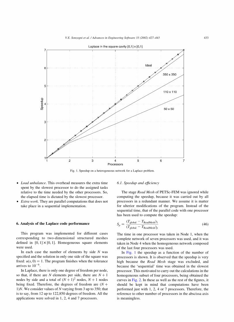
In Fig. 1 the speedup as a function of the number of

processors is shown. It is observed that the speedup is very

high because the Read Mesh stage was excluded, and

because the ‘sequential’ time was obtained in the slowest

processor. This motivated to carry out the calculations in the

homogeneous subset of four processors, being obtained the

curves in Fig. 2. In these as well as the rest of the figures, it

should be kept in mind that computations have been

performed just with 1, 2, 4 or 7 processors. Therefore, the

reference to other number of processors in the abscissa axis

is meaningless.

Fig. 1. Speedup on a heterogeneous network for a Laplace problem.

V.E. Sonzogni et al. / Advances in Engineering Software 33 (2002) 427–443 433

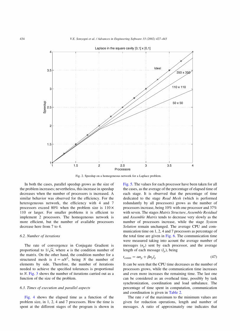
In both the cases, parallel speedup grows as the size of

the problem increases; nevertheless, this increase in speedup

decreases when the number of processors is increased. A

similar behavior was observed for the efficiency. For the

heterogeneous network, the efficiency with 4 and 7

processors exceed 80% when the problem size is 110 £

110 or larger. For smaller problems it is efficient to

implement 2 processors. The homogeneous network is

more efficient, but the number of available processors

decrease here from 7 to 4.

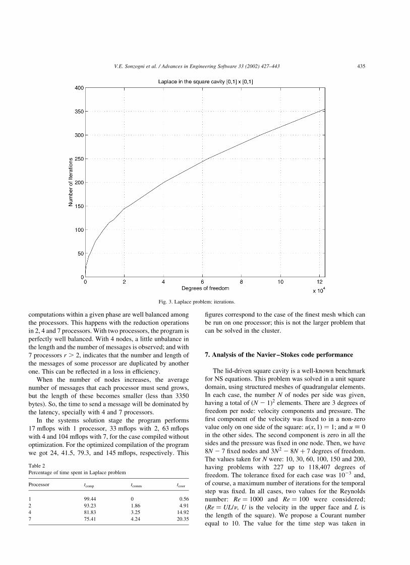
6.2. Number of iterations

The rate of convergence in Conjugate Gradient is

proportional to 1=ffiffik

p; where k is the condition number of

the matrix. On the other hand, the condition number for a

structured mesh is k ¼ aN2; being N the number of

elements by side. Therefore, the number of iterations

needed to achieve the specified tolerances is proportional

to N. Fig. 3 shows the number of iterations carried out as a

function of the size of the problem.

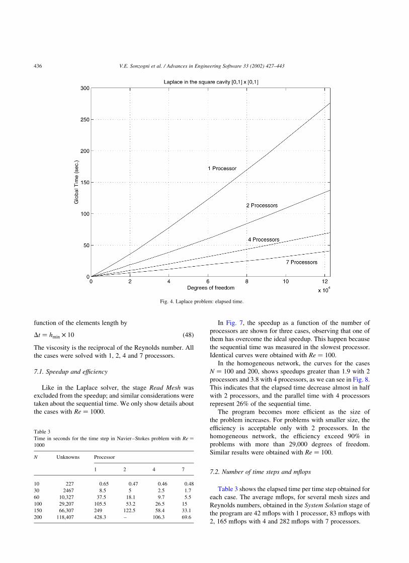
6.3. Times of execution and parallel aspects

Fig. 4 shows the elapsed time as a function of the

problem size, in 1, 2, 4 and 7 processors. How the time is

spent at the different stages of the program is shown in

Fig. 5. The values for each processor have been taken for all

the cases, as the average of the percentage of elapsed time of

each stage. It is observed that the percentage of time

dedicated to the stage Read Mesh (which is performed

redundantly by all processors) grows as the number of

processors increase, being 10% with one processor and 37%

with seven. The stages Matrix Structure, Assemble Residual

and Assemble Matrix tends to decrease very slowly as the

number of processors increase, while the stage System

Solution remain unchanged. The average CPU and com-

munication time on 1, 2, 4 and 7 processors as percentage of

the total time are given in Fig. 6. The communication time

were measured taking into acount the average number of

messages ðnpÞ sent by each processor, and the average

length of each message ðlpÞ; being

tcomm ¼ anp þ bnplp ð47Þ

It can be seen that the CPU time decreases as the number of

processors grows, while the communication time increases

and even more increases the remaining time. The last one

can be considered as an overhead time, possibly by task

synchronization, coordination and load unbalance. The

percentage of time spent in computation, communication

and coordination is given in Table 2.

The rate r of the maximum to the minimum values are

given for reduction operations, length and number of

messages. A ratio of approximately one indicates that

Fig. 2. Speedup on a homogeneous network for a Laplace problem.

V.E. Sonzogni et al. / Advances in Engineering Software 33 (2002) 427–443434

computations within a given phase are well balanced among

the processors. This happens with the reduction operations

in 2, 4 and 7 processors. With two processors, the program is

perfectly well balanced. With 4 nodes, a little unbalance in

the length and the number of messages is observed; and with

7 processors r . 2; indicates that the number and length of

the messages of some processor are duplicated by another

one. This can be reflected in a loss in efficiency.

When the number of nodes increases, the average

number of messages that each processor must send grows,

but the length of these becomes smaller (less than 3350

bytes). So, the time to send a message will be dominated by

the latency, specially with 4 and 7 processors.

In the systems solution stage the program performs

17 mflops with 1 processor, 33 mflops with 2, 63 mflops

with 4 and 104 mflops with 7, for the case compiled without

optimization. For the optimized compilation of the program

we got 24, 41.5, 79.3, and 145 mflops, respectively. This

figures correspond to the case of the finest mesh which can

be run on one processor; this is not the larger problem that

can be solved in the cluster.

7. Analysis of the Navier–Stokes code performance

The lid-driven square cavity is a well-known benchmark

for NS equations. This problem was solved in a unit square

domain, using structured meshes of quadrangular elements.

In each case, the number N of nodes per side was given,

having a total of ðN 2 1Þ2 elements. There are 3 degrees of

freedom per node: velocity components and pressure. The

first component of the velocity was fixed to in a non-zero

value only on one side of the square: uðx; 1Þ ¼ 1; and u ; 0

in the other sides. The second component is zero in all the

sides and the pressure was fixed in one node. Then, we have

8N 2 7 fixed nodes and 3N2 2 8N þ 7 degrees of freedom.

The values taken for N were: 10, 30, 60, 100, 150 and 200,

having problems with 227 up to 118,407 degrees of

freedom. The tolerance fixed for each case was 1023 and,

of course, a maximum number of iterations for the temporal

step was fixed. In all cases, two values for the Reynolds

number: Re ¼ 1000 and Re ¼ 100 were considered;

(Re ¼ UL=n; U is the velocity in the upper face and L is

the length of the square). We propose a Courant number

equal to 10. The value for the time step was taken in

Fig. 3. Laplace problem: iterations.

Table 2

Percentage of time spent in Laplace problem

Processor tcomp tcomm tcoor

1 99.44 0 0.56

2 93.23 1.86 4.91

4 81.83 3.25 14.92

7 75.41 4.24 20.35

V.E. Sonzogni et al. / Advances in Engineering Software 33 (2002) 427–443 435

function of the elements length by

Dt ¼ hmin £ 10 ð48Þ

The viscosity is the reciprocal of the Reynolds number. All

the cases were solved with 1, 2, 4 and 7 processors.

7.1. Speedup and efficiency

Like in the Laplace solver, the stage Read Mesh was

excluded from the speedup; and similar considerations were

taken about the sequential time. We only show details about

the cases with Re ¼ 1000:

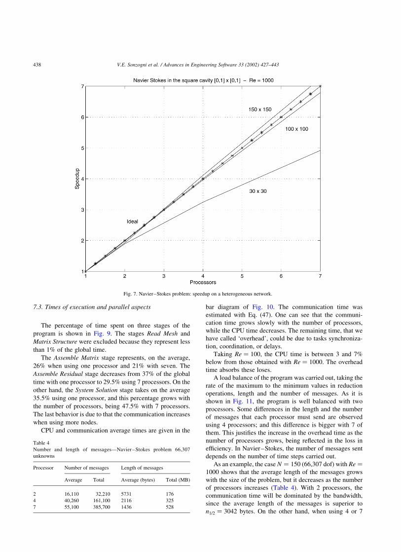
In Fig. 7, the speedup as a function of the number of

processors are shown for three cases, observing that one of

them has overcome the ideal speedup. This happen because

the sequential time was measured in the slowest processor.

Identical curves were obtained with Re ¼ 100:

In the homogeneous network, the curves for the cases

N ¼ 100 and 200, shows speedups greater than 1.9 with 2

processors and 3.8 with 4 processors, as we can see in Fig. 8.

This indicates that the elapsed time decrease almost in half

with 2 processors, and the parallel time with 4 processors

represent 26% of the sequential time.

The program becomes more efficient as the size of

the problem increases. For problems with smaller size, the

efficiency is acceptable only with 2 processors. In the

homogeneous network, the efficiency exceed 90% in

problems with more than 29,000 degrees of freedom.

Similar results were obtained with Re ¼ 100:

7.2. Number of time steps and mflops

Table 3 shows the elapsed time per time step obtained for

each case. The average mflops, for several mesh sizes and

Reynolds numbers, obtained in the System Solution stage of

the program are 42 mflops with 1 processor, 83 mflops with

2, 165 mflops with 4 and 282 mflops with 7 processors.

Fig. 4. Laplace problem: elapsed time.

Table 3

Time in seconds for the time step in Navier–Stokes problem with Re ¼

1000

N Unknowns Processor

1 2 4 7

10 227 0.65 0.47 0.46 0.48

30 2467 8.5 5 2.5 1.7

60 10,327 37.5 18.1 9.7 5.5

100 29,207 105.5 53.2 26.5 15

150 66,307 249 122.5 58.4 33.1

200 118,407 428.3 – 106.3 69.6

V.E. Sonzogni et al. / Advances in Engineering Software 33 (2002) 427–443436

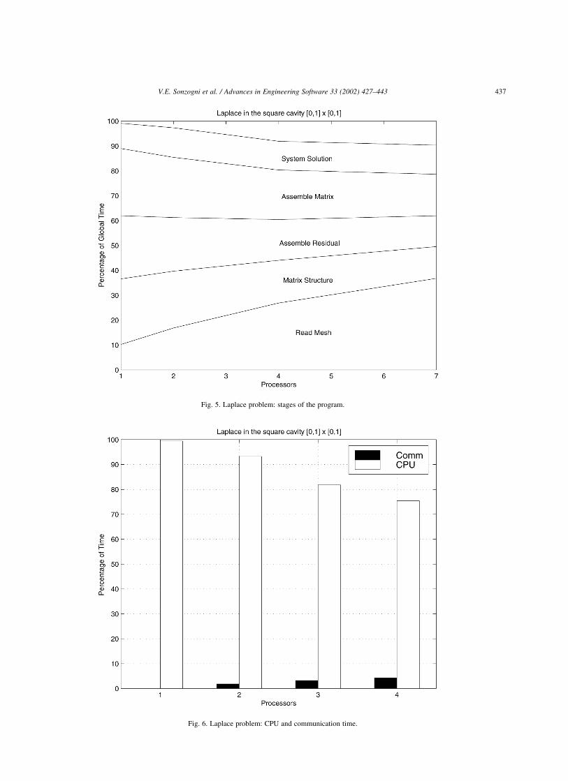
Fig. 5. Laplace problem: stages of the program.

Fig. 6. Laplace problem: CPU and communication time.

V.E. Sonzogni et al. / Advances in Engineering Software 33 (2002) 427–443 437

7.3. Times of execution and parallel aspects

The percentage of time spent on three stages of the

program is shown in Fig. 9. The stages Read Mesh and

Matrix Structure were excluded because they represent less

than 1% of the global time.

The Assemble Matrix stage represents, on the average,

26% when using one processor and 21% with seven. The

Assemble Residual stage decreases from 37% of the global

time with one processor to 29:5% using 7 processors. On the

other hand, the System Solution stage takes on the average

35:5% using one processor, and this percentage grows with

the number of processors, being 47:5% with 7 processors.

The last behavior is due to that the communication increases

when using more nodes.

CPU and communication average times are given in the

bar diagram of Fig. 10. The communication time was

estimated with Eq. (47). One can see that the communi-

cation time grows slowly with the number of processors,

while the CPU time decreases. The remaining time, that we

have called ‘overhead’, could be due to tasks synchroniza-

tion, coordination, or delays.

Taking Re ¼ 100; the CPU time is between 3 and 7%

below from those obtained with Re ¼ 1000: The overhead

time absorbs these loses.

A load balance of the program was carried out, taking the

rate of the maximum to the minimum values in reduction

operations, length and the number of messages. As it is

shown in Fig. 11, the program is well balanced with two

processors. Some differences in the length and the number

of messages that each processor must send are observed

using 4 processors; and this difference is bigger with 7 of

them. This justifies the increase in the overhead time as the

number of processors grows, being reflected in the loss in

efficiency. In Navier–Stokes, the number of messages sent

depends on the number of time steps carried out.

As an example, the case N ¼ 150 (66,307 dof) with Re ¼

1000 shows that the average length of the messages grows

with the size of the problem, but it decreases as the number

of processors increases (Table 4). With 2 processors, the

communication time will be dominated by the bandwidth,

since the average length of the messages is superior to

n1=2 ¼ 3042 bytes. On the other hand, when using 4 or 7

Fig. 7. Navier–Stokes problem: speedup on a heterogeneous network.

Table 4

Number and length of messages—Navier–Stokes problem 66,307

unknowns

Processor Number of messages Length of messages

Average Total Average (bytes) Total (MB)

2 16,110 32,210 5731 176

4 40,260 161,100 2116 325

7 55,100 385,700 1436 528

V.E. Sonzogni et al. / Advances in Engineering Software 33 (2002) 427–443438

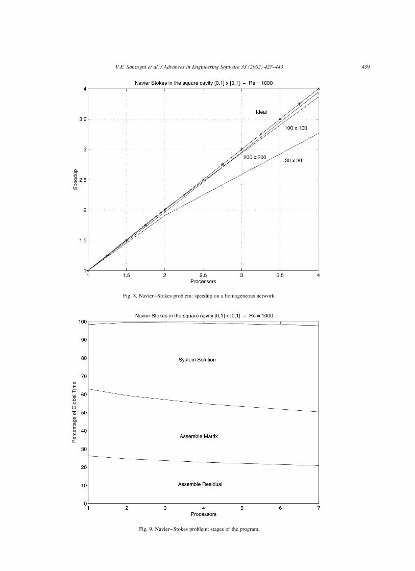
Fig. 8. Navier–Stokes problem: speedup on a homogeneous network.

Fig. 9. Navier–Stokes problem: stages of the program.

V.E. Sonzogni et al. / Advances in Engineering Software 33 (2002) 427–443 439

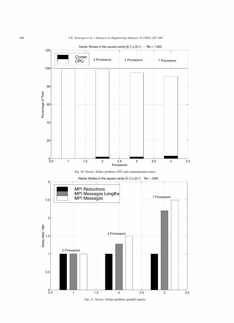
Fig. 10. Navier–Stokes problem: CPU and communication times.

Fig. 11. Navier–Stokes problem: parallel aspects.

V.E. Sonzogni et al. / Advances in Engineering Software 33 (2002) 427–443440

processors, the communication time will be dominated by

the latency. In this particular case, 100 iterations of the time

step have been done, showing that each processor sent, on

the average, 161, 403 or 551 messages, either in 2, 4 or 7

processors, respectively.

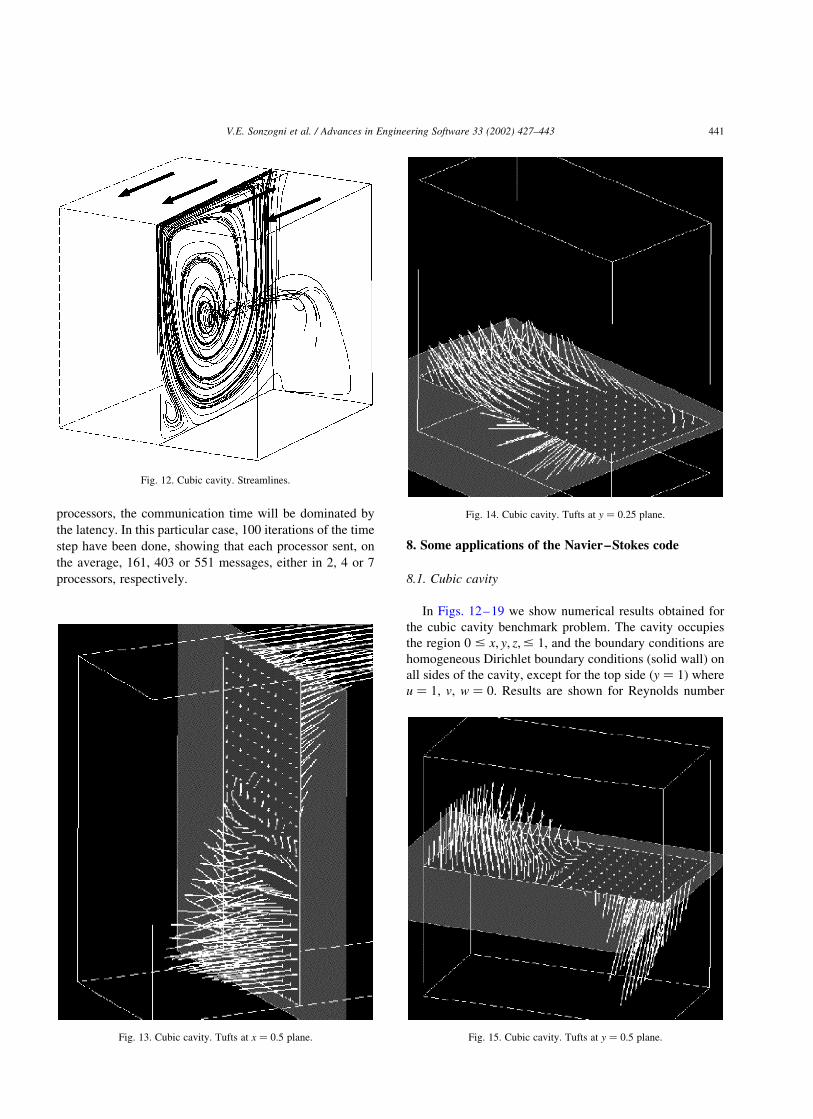
8. Some applications of the Navier–Stokes code

8.1. Cubic cavity

In Figs. 12–19 we show numerical results obtained for

the cubic cavity benchmark problem. The cavity occupies

the region 0 # x; y; z;# 1; and the boundary conditions are

homogeneous Dirichlet boundary conditions (solid wall) on

all sides of the cavity, except for the top side ðy ¼ 1Þ where

u ¼ 1; v; w ¼ 0: Results are shown for Reynolds number

Fig. 12. Cubic cavity. Streamlines.

Fig. 13. Cubic cavity. Tufts at x ¼ 0:5 plane.

Fig. 14. Cubic cavity. Tufts at y ¼ 0:25 plane.

Fig. 15. Cubic cavity. Tufts at y ¼ 0:5 plane.

V.E. Sonzogni et al. / Advances in Engineering Software 33 (2002) 427–443 441

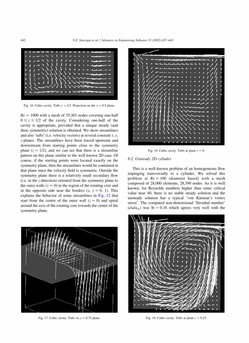
Re ¼ 1000 with a mesh of 35,301 nodes covering one-half

0 # z # 1=2 of the cavity. Considering one-half of the

cavity is appropriate, provided that a unique steady (and

then, symmetric) solution is obtained. We show streamlines

and also ‘tufts’ (i.e. velocity vectors) at several constant x; y;

z-planes. The streamlines have been traced upstream and

downstream from starting points close to the symmetry

plane ðz ¼ 1=2Þ; and we can see that there is a streamline

pattern on this plane similar to the well known 2D case. Of

course, if the starting points were located exactly on the

symmetry plane, then the streamlines would be contained in

that plane since the velocity field is symmetric. Outside the

symmetry plane there is a relatively small secondary flow

(i.e. in the z-direction) oriented from the symmetry plane to

the outer walls ðz ¼ 0Þ in the region of the rotating core and

in the opposite side near the borders ðx; y ¼ 0; 1Þ: This

explains the behavior of some streamlines in Fig. 12 that

start from the center of the outer wall ðz ¼ 0Þ and spiral

around the axis of the rotating core towards the center of the

symmetry plane.

8.2. Unsteady 2D cylinder

This is a well-known problem of an homogeneous flow

impinging transversally to a cylinder. We solved this

problem at Re ¼ 100 (diameter based) with a mesh

composed of 28,000 elements, 28,390 nodes. As it is well

known, for Reynolds numbers higher than some critical

value near 40, there is no stable steady solution and the

unsteady solution has a typical ‘von Karman’s vortex

street’. The computed non-dimensional ‘Strouhal number’

ðdv=u1Þ was St ¼ 0:16 which agrees very well with the

Fig. 16. Cubic cavity. Tufts y ¼ 0:5: Projection on the y ¼ 0:5 plane.

Fig. 17. Cubic cavity. Tufts on y ¼ 0:75 plane.

Fig. 18. Cubic cavity. Tufts at plane z ¼ 0:

Fig. 19. Cubic cavity. Tufts at plane z ¼ 0:25:

V.E. Sonzogni et al. / Advances in Engineering Software 33 (2002) 427–443442

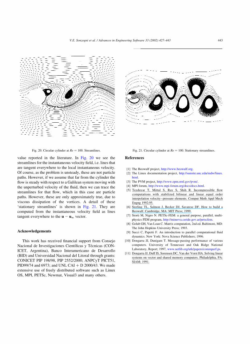
value reported in the literature. In Fig. 20 we see the

streamlines for the instantaneous velocity field, i.e. lines that

are tangent everywhere to the local instantaneous velocity.

Of course, as the problem is unsteady, these are not particle

paths. However, if we assume that far from the cylinder the

flow is steady with respect to a Galilean system moving with

the unperturbed velocity of the fluid, then we can trace the

streamlines for that flow, which in this case are particle

paths. However, these are only approximately true, due to

viscous dissipation of the vortices. A detail of these

‘stationary streamlines’ is shown in Fig. 21. They are

computed from the instantaneous velocity field as lines

tangent everywhere to the u 2 u1 vector.

Acknowledgements

This work has received financial support from Consejo

Nacional de Investigaciones Cientıficas y Tecnicas (CON-

ICET, Argentina), Banco Interamericano de Desarrollo

(BID) and Universidad Nacional del Litoral through grants:

CONICET PIP 198/98, PIP 2552/2000; ANPCyT PICT51,

PID99/74 and 6973; and UNL CAI þ D 2000/43. We made

extensive use of freely distributed software such as Linux

OS, MPI, PETSc, Newmat, Visual3 and many others.

References

[1] The Beowulf project, http://www.beowulf.org.

[2] The Linux documentation project, http://sunsite.unc.edu/mdw/linux.

html.

[3] The PVM project, http://www.epm.ornl.gov/pvm/.

[4] MPI forum, http://www.mpi-forum.org/docs/docs.html.

[5] Tezduyar T, Mittal S, Ray S, Shih R. Incompressible flow

computations with stabilized bilinear and linear equal order

interpolation velocity–pressure elements. Comput Meth Appl Mech

Engng 1992;95.

[6] Sterling TL, Salmon J, Becker DJ, Savarese DF. How to build a

Beowulf. Cambridge, MA: MIT Press; 1999.

[7] Storti M, Nigro N. PETSc-FEM: a general purpose, parallel, multi-

physics FEM program, http://minerva.ceride.gov.ar/petscfem.

[8] Golub GH, Van Loan C. Matrix computation, 2nd ed. Baltimore, MD:

The John Hopkins University Press; 1993.

[9] Succi C, Papetti F. An introduction to parallel computational fluid

dynamics. New York: Nova Science Publishers; 1996.

[10] Dongarra JJ, Dunigam T. Message-passing performance of various

computers. University of Tennessee and Oak Ridge National

Laboratory, Report; 1997, www.netlib.org/utk/papers/commperf.ps.

[11] Dongarra JJ, Duff IS, Sorensen DC, Van der Vorst HA. Solving linear

systems on vector and shared memory computers. Philadelphia, PA:

SIAM; 1991.

Fig. 20. Circular cylinder at Re ¼ 100: Streamlines. Fig. 21. Circular cylinder at Re ¼ 100: Stationary streamlines.

V.E. Sonzogni et al. / Advances in Engineering Software 33 (2002) 427–443 443