A numerical study of the spectral gap

This article has been downloaded from IOPscience. Please scroll down to see the full text article.

2008 J. Phys. A: Math. Theor. 41 055201

(http://iopscience.iop.org/1751-8121/41/5/055201)

Download details:

IP Address: 193.137.5.230

The article was downloaded on 20/07/2011 at 15:20

Please note that terms and conditions apply.

View the table of contents for this issue, or go to the journal homepage for more

Home Search Collections Journals About Contact us My IOPscience

IOP PUBLISHING JOURNAL OF PHYSICS A: MATHEMATICAL AND THEORETICAL

J. Phys. A: Math. Theor. 41 (2008) 055201 (19pp) doi:10.1088/1751-8113/41/5/055201

A numerical study of the spectral gap

Pedro Antunes1 and Pedro Freitas2

1 CEMAT, Instituto Superior Tecnico (TU Lisbon), Av.Rovisco Pais, 1049-001 Lisboa, Portugal2 Departamento de Matematica, Faculdade de Motricidade Humana (TU Lisbon) and Group ofMathematical Physics of the University of Lisbon, Complexo Interdisciplinar, Av. Prof. GamaPinto 2, P-1649-003 Lisboa, Portugal

E-mail: pant@math.ist.utl.pt and freitas@cii.fc.ul.pt

Received 6 August 2007, in final form 13 December 2007Published 23 January 2008Online at stacks.iop.org/JPhysA/41/055201

AbstractWe present a numerical study of the spectral gap of the Dirichlet Laplacian,γ (K) = λ2(K) − λ1(K), of a planar convex region K. Besides providingsupporting numerical evidence for the long-standing gap conjecture thatγ (K) � 3π2/d2(K), where d(K) denotes the diameter of K, our study suggestsnew types of bounds and several conjectures regarding the dependence of thegap not only on the diameter, but also on the perimeter and the area. Oneof these conjectures is a stronger version of the gap conjecture mentionedabove. A similar study is carried out for the quotient of the first two Dirichleteigenvalues.

PACS numbers: 02.30.Jr, 02.70.HmMathematics Subject Classification: 35P15, 58G25

1. Introduction

This is the second in a series of papers consisting of a numerical study of several issues relatedto the spectrum of the Laplace operator. The main purpose of this program is to unveil someof the structure behind the connection between the low eigenvalues and certain elementarygeometric quantities such as the perimeter, the area and the diameter. Many relations of thistype are, of course, known, but it is our belief that they may still be improved in many casesand that at this stage this is best done with the help of numerical insight. This is due to the factthat some of the expressions obtained are quite involved, although they appear quite naturallywhen seen from the appropriate point of view—see, for instance, conjectures 7, 10, 15 and 17below.

To illustrate our point, and also because of the connection with the present work, letus consider one of the conjectures that resulted from our previous work [AF]. There weconsidered the first Dirichlet eigenvalue and studied this quantity on polygons. This led us to

1751-8113/08/055201+19$30.00 © 2008 IOP Publishing Ltd Printed in the UK 1

J. Phys. A: Math. Theor. 41 (2008) 055201 P Antunes and P Freitas

the following conjecture which, if true, is an improvement of a result by Payne and Weinberger[PW].

Conjecture 1. For any planar simply connected domain � we have

λ1(�) � πj 201

A+

π2

4

L2 − 4πA

A2 ,

where L and A denote the perimeter and the area of �, respectively.

Inequalities of this type are not surprising in themselves, as they are simply a translation ofthe fact that there is an obvious relation between eigenvalues and the geometrical quantitiesinvolved. However, most of the classical results such as the Faber–Krahn inequality are whatwe might call static, in that they do not take into account how far we are from the optimal setin geometric terms. In the above case, the natural way of measuring this is by consideringthe isoperimetric defect L2 − 4πA, and so we looked for the possibility of bounding the firsteigenvalue by an expression of the form

πj 201

A+ C

L2 − 4πA

A2, (1)

where the constant C was to be determined. We remark that the introduction of such termshas a counterpart in classical geometry where, for instance, there exist improvements of theclassical geometric isoperimetric inequality with defect terms, such as Bonnesen’s inequality—see [BZ] for several examples of this type. For other types of correction terms see, for instance,[FK, M].

Note that at first it is not clear that an inequality for λ1 involving the term (1) shouldexist, nor that it should provide a lower or an upper bound. One of the surprising results in[AF] was precisely the fact that, within each class of n-polygons, the expression above (withthe isoperimetric defect for a general domain replaced by that for n-polygons) does seem toprovide both lower and upper bounds for the first Dirichlet eigenvalue if the constant C ischosen appropriately—see [AF] for more details. It turned out that while the upper boundconverged to that in conjecture 1 as n went to infinity, the lower bound seemed to converge tothat which is given by the Faber–Krahn inequality.

Another key ingredient leading to conjecture 1 was the identification of the extremal sets,that is, sets for which the inequality becomes an identity. While the ball is an obvious solutionto this problem, the fact that we have an extra parameter suggested that there should exist otherextremal sets whose nature is not so obvious a priori—see [AF] for the conjectured extremalsets under the restriction to families of n-polygons. In the case of upper bounds of the form(1) for general simply-connected domains the other extremal sets are what might be calledasymptotical extremal sets, namely, a rectangle for which one side length is kept fixed whilethe other goes to infinity. Note that balls and infinite strips are the only planar domains with asmooth boundary having constant curvature.

An important issue here is that the infinite strips described above which are asymptoticalextremal sets in conjecture 1 are also asymptotical extremal sets for the following gapconjecture,

Conjecture 2. For any planar convex domain K we have

γ (K) := λ2(K) − λ1(K) � 3π2

d2,

where d denotes the diameter of K.

2

J. Phys. A: Math. Theor. 41 (2008) 055201 P Antunes and P Freitas

This conjecture has a long history which may be traced back to [Be] in the context ofa free boson gas confined in a region in n-dimensional Euclidean space by a container withhard walls, and has received much attention during the intervening time. The conjecture isknown to be true in the case of planar domains which are convex and symmetric with respectto two perpendicular axis [BK, D]. For other progress on this in the case of general convexdomains see [SWYY, Sm, YZ], for instance, and the report [A] which contains an extensivebibliography on the subject.

All of the above suggested the performance in the case of the gap of a study similar tothat which had been carried out in [AF], and, in particular, to check if it is possible to obtain abound where besides infinite strips we also get equality for other domains. At a more generallevel, the purpose of the present paper is to understand the behaviour of certain functionalsof the first two Dirichlet eigenvalues. More precisely, we shall consider the Dirichlet spectralgap and also mention briefly the spectral quotient defined for a domain � in R2 by

ξ(�) := λ2(�)

λ1(�). (2)

Apart from the fact that the spectral gap plays an important role in several areas of mathematicalphysics, the two functionals γ and ξ were chosen as the simplest examples where there are twoeffects pulling in opposite directions and where we expect at least some of the behaviour to bequite different—recall, for instance, that while the gap conjecture only makes sense for convexdomains, in the case of ξ we know that it satisfies a static inequality of the Faber–Krahn type,namely, ξ(�) � ξ(B). This was conjectured by Payne, Polya and Weinberger [PPW] in 1956and was finally proved by Ashbaugh and Benguria in [AB], approximately 35 years later. Inconnection to this, we point out that the paper [Si] contains some isoperimetric inequalitiessimilar to this for the spectral gap and quotient of triangles. There are also several otherfunctionals of this type which have been considered in the literature. In [LY], for instance,the authors carried out a numerical study where besides ξ they also considered the quotientλ3/λ1.

A general outcome of our work is that one should expect the existence of similar resultsto those for the first Dirichlet eigenvalue for both γ and ξ . More precisely, we conjecturethat there exist inequalities depending on geometrical quantities such as the perimeter and thearea or the diameter and the area for which the extremal sets are the same as those mentionedabove for the first Dirichlet eigenvalue, namely, balls and asymptotically on infinite strips.Furthermore, our results show that indeed there seems to be a very close relationship betweenthe spectral gap and the diameter. This can be seen from the fact that within the class ofn-polygons the optimal polygon is the same as the optimal polygon for geometric isodiametricinequalities—see section 3.1 below. Finally, we also detected that certain types of isoscelestriangles play a role as extremal sets under certain conditions, in the sense that they seem tobound the possible values of the gap and the quotient from above. We also identified othersets in these conditions—see sections 3 and 4.

The method of study employed here is similar to that used in [AF]. More precisely,we begin by analysing some cases where the quantities involved are known explicitly, andrewrite the eigenvalues as a function of the geometric quantities mentioned above. Since forsome of the problems considered balls and rectangles correspond to extremal domains, thisallows us to obtain expressions for possible bounds directly. In other situations, such as whenwe have dependence on the diameter, rectangles turned out not to be extremal domains butthe explicit expression obtained for them was still useful to understand the form the boundshould take. These explicit expressions are then checked against a large sample of randomlygenerated planar domains consisting mainly of polygons with a small number of sides—ourdatabase has over 50.000 randomly generated convex polygons, of which nearly one eighth are

3

J. Phys. A: Math. Theor. 41 (2008) 055201 P Antunes and P Freitas

(non-degenerate) octagons. Based on the numerical evidence we either discard the expressionas a possible bound, or, in the case of positive results, proceed to test it against polygons witha larger number of sides and, in some cases such as the bounds for ξ , against non-convexpolygons. In other cases we analysed the clouds of points generated for the gap and thequotient for a given class of polygons as functions of the perimeter or the diameter, andproceeded to identify the domains corresponding to the points on the boundary of these sets.The necessary computations to deal with such a large number of domains are quite heavy, andthe eigenvalue calculation was done using the method of fundamental solutions which allowsfor such a treatment—see [AA] for details. For a different numerical approach see [TB].

The organization of the paper is as follows. Section 2 contains a study of some basicproperties of the gap, such as (lack of) monotonicity, unboundedness, etc. Section 3 containsthe numerical study of the gap, where we address its dependence on diameter, perimeter andarea. In section 4 we mention some results from a similar study for the quotient of the firsttwo eigenvalues. Finally, in section 5 we discuss the results obtained.

2. Some basic results for the gap

2.1. Unboundedness

We begin by recalling that γ (K) is not bounded from above neither among convex planarsets of fixed diameter, nor among those of fixed area. This may already be found in [Sm],and it is a direct consequence of the fact that, for sufficiently small β, the first and secondeigenvalues of the circular sector of angle opening β and radius r, Sβ,r , are given by j 2

πβ,1

/r2

and j 2πβ,2

/r2, respectively. On the other hand, the zeros jν,i(i = 1, 2) have the following

asymptotic expansions as ν approaches infinity [EF]:

jν,i = ν − ai

21/3ν1/3 + O(ν−1/3), i = 1, 2.

Hence

γ (Sβ,r ) = 22/3 a1 − a2

r2

(π

β

)4/3

+ O(β−2/3), as β → 0,

where a1 ≈ −2.338 11 and a2 ≈ −4.087 95 are the first and second negative zeros of the Airyfunction of the first kind, respectively.

Note that for β smaller than π/3 we have d(Sβ,r ) = r independently of β, and so thisprovides an example where the gap converges to infinity while keeping the diameter fixed. Tosee that it also yields that the gap is unbounded in the case of the fixed area problem, notethat A(Sβ,r ) = βr2/2 and we should thus take r equal to (2A/β)1/2 in order to keep the areaconstant. This gives

γ (Sβ,( 2Aβ

)1/2) = a1 − a2

21/3A

π4/3

β1/3+ O(β1/3), as β → 0.

Similar results may be obtained for other domains such as isosceles triangles and rhombi—see [F]. Note that this unbounded behaviour for fixed area in the thin limit case dependson smoothness assumptions of the domain, as it has been shown in [BF] that under somesmoothness constraints the quantity A(�ε)γ (�ε) will remain bounded as ε goes to zero,where �ε denotes a domain that is being shrunk in one direction.

None of the above means, of course, that there are no local maxima for the gap, and thiswill indeed be the case as we will see below. On the other hand, it shows that the behaviourof γ is indeed quite different from that of ξ , at least in this respect.

4

J. Phys. A: Math. Theor. 41 (2008) 055201 P Antunes and P Freitas

0.5 1 1.5 2

0.20.40.60.8

1

0.5 1 1.5 2

0.20.40.60.8

1

0.5 1 1.5 2

0.20.40.60.8

1

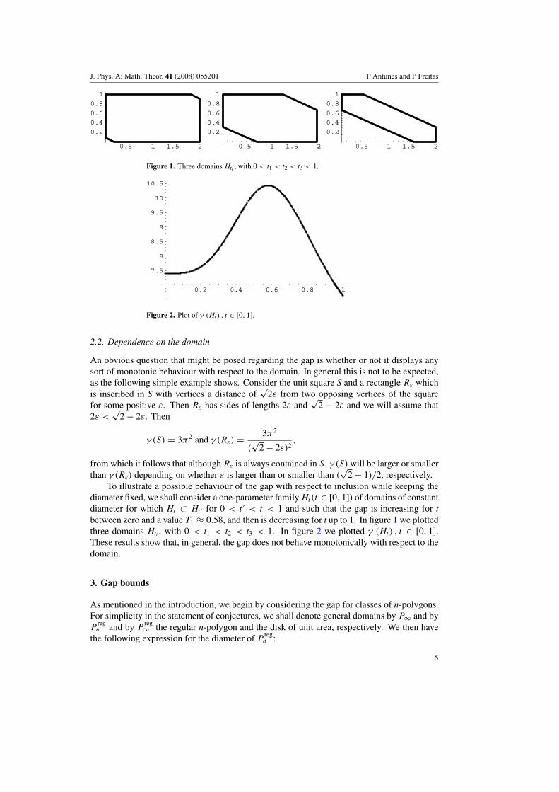
Figure 1. Three domains Hti , with 0 < t1 < t2 < t3 < 1.

0.2 0.4 0.6 0.8 1

7.5

8

8.5

9

9.5

10

10.5

Figure 2. Plot of γ (Ht ) , t ∈ [0, 1].

2.2. Dependence on the domain

An obvious question that might be posed regarding the gap is whether or not it displays anysort of monotonic behaviour with respect to the domain. In general this is not to be expected,as the following simple example shows. Consider the unit square S and a rectangle Rε whichis inscribed in S with vertices a distance of

√2ε from two opposing vertices of the square

for some positive ε. Then Rε has sides of lengths 2ε and√

2 − 2ε and we will assume that2ε <

√2 − 2ε. Then

γ (S) = 3π2 and γ (Rε) = 3π2

(√

2 − 2ε)2,

from which it follows that although Rε is always contained in S, γ (S) will be larger or smallerthan γ (Rε) depending on whether ε is larger than or smaller than (

√2 − 1)/2, respectively.

To illustrate a possible behaviour of the gap with respect to inclusion while keeping thediameter fixed, we shall consider a one-parameter family Ht(t ∈ [0, 1]) of domains of constantdiameter for which Ht ⊂ Ht ′ for 0 < t ′ < t < 1 and such that the gap is increasing for tbetween zero and a value T1 ≈ 0.58, and then is decreasing for t up to 1. In figure 1 we plottedthree domains Hti , with 0 < t1 < t2 < t3 < 1. In figure 2 we plotted γ (Ht) , t ∈ [0, 1].These results show that, in general, the gap does not behave monotonically with respect to thedomain.

3. Gap bounds

As mentioned in the introduction, we begin by considering the gap for classes of n-polygons.For simplicity in the statement of conjectures, we shall denote general domains by P∞ and byP

regn and by P

reg∞ the regular n-polygon and the disk of unit area, respectively. We then have

the following expression for the diameter of Pregn :

5

J. Phys. A: Math. Theor. 41 (2008) 055201 P Antunes and P Freitas

3 4 5 6

5

10

15

20

25

30

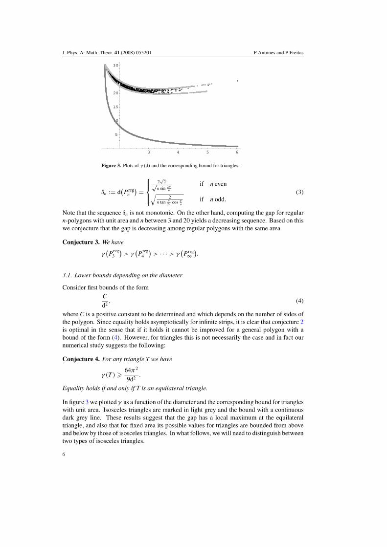
Figure 3. Plots of γ (d) and the corresponding bound for triangles.

δn := d(P reg

n

) =

⎧⎪⎨⎪⎩

2√

2√n sin 2π

n

if n even√2

n tan π2n

cos πn

if n odd.(3)

Note that the sequence δn is not monotonic. On the other hand, computing the gap for regularn-polygons with unit area and n between 3 and 20 yields a decreasing sequence. Based on thiswe conjecture that the gap is decreasing among regular polygons with the same area.

Conjecture 3. We have

γ(P

reg3

)> γ

(P

reg4

)> · · · > γ

(P reg

∞).

3.1. Lower bounds depending on the diameter

Consider first bounds of the formC

d2, (4)

where C is a positive constant to be determined and which depends on the number of sides ofthe polygon. Since equality holds asymptotically for infinite strips, it is clear that conjecture 2is optimal in the sense that if it holds it cannot be improved for a general polygon with abound of the form (4). However, for triangles this is not necessarily the case and in fact ournumerical study suggests the following:

Conjecture 4. For any triangle T we have

γ (T ) � 64π2

9d2.

Equality holds if and only if T is an equilateral triangle.

In figure 3 we plotted γ as a function of the diameter and the corresponding bound for triangleswith unit area. Isosceles triangles are marked in light grey and the bound with a continuousdark grey line. These results suggest that the gap has a local maximum at the equilateraltriangle, and also that for fixed area its possible values for triangles are bounded from aboveand below by those of isosceles triangles. In what follows, we will need to distinguish betweentwo types of isosceles triangles.

6

J. Phys. A: Math. Theor. 41 (2008) 055201 P Antunes and P Freitas

3 4 5 6 7

10

15

20

25

30

A=0.9

A=1

A=1.1

A=1.2

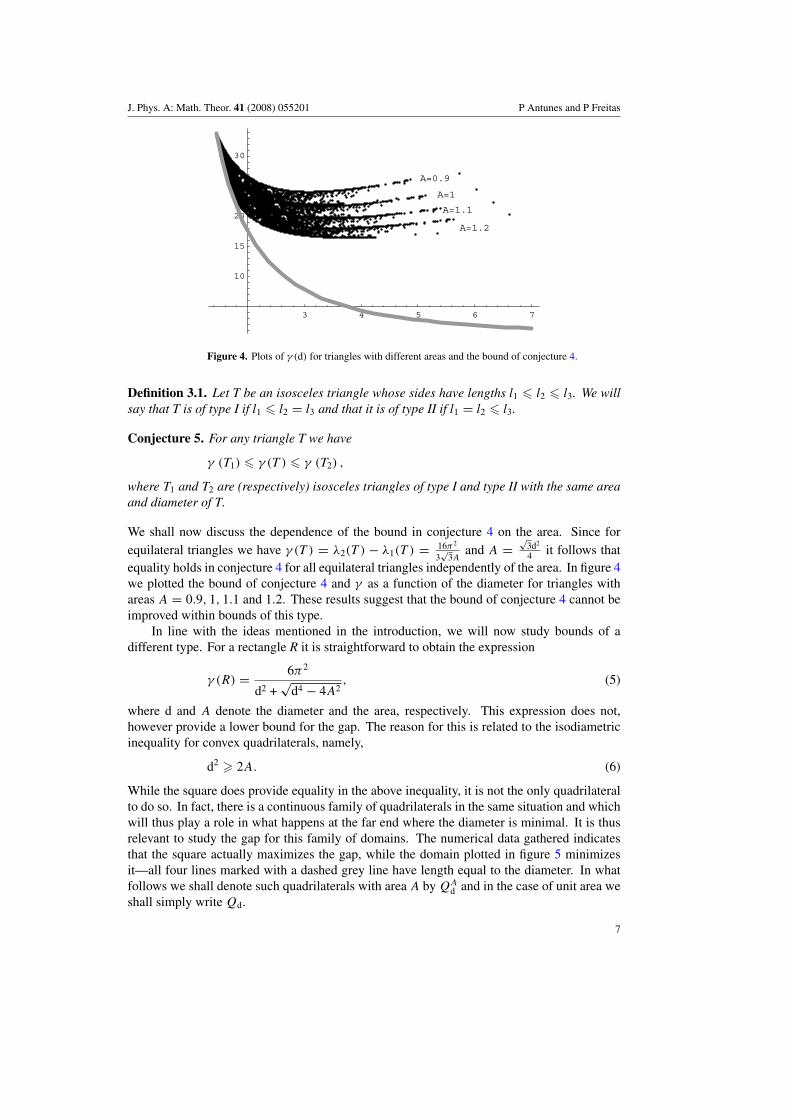
Figure 4. Plots of γ (d) for triangles with different areas and the bound of conjecture 4.

Definition 3.1. Let T be an isosceles triangle whose sides have lengths l1 � l2 � l3. We willsay that T is of type I if l1 � l2 = l3 and that it is of type II if l1 = l2 � l3.

Conjecture 5. For any triangle T we have

γ (T1) � γ (T ) � γ (T2) ,

where T1 and T2 are (respectively) isosceles triangles of type I and type II with the same areaand diameter of T.

We shall now discuss the dependence of the bound in conjecture 4 on the area. Since forequilateral triangles we have γ (T ) = λ2(T ) − λ1(T ) = 16π2

3√

3Aand A =

√3d2

4 it follows thatequality holds in conjecture 4 for all equilateral triangles independently of the area. In figure 4we plotted the bound of conjecture 4 and γ as a function of the diameter for triangles withareas A = 0.9, 1, 1.1 and 1.2. These results suggest that the bound of conjecture 4 cannot beimproved within bounds of this type.

In line with the ideas mentioned in the introduction, we will now study bounds of adifferent type. For a rectangle R it is straightforward to obtain the expression

γ (R) = 6π2

d2 +√

d4 − 4A2, (5)

where d and A denote the diameter and the area, respectively. This expression does not,however provide a lower bound for the gap. The reason for this is related to the isodiametricinequality for convex quadrilaterals, namely,

d2 � 2A. (6)

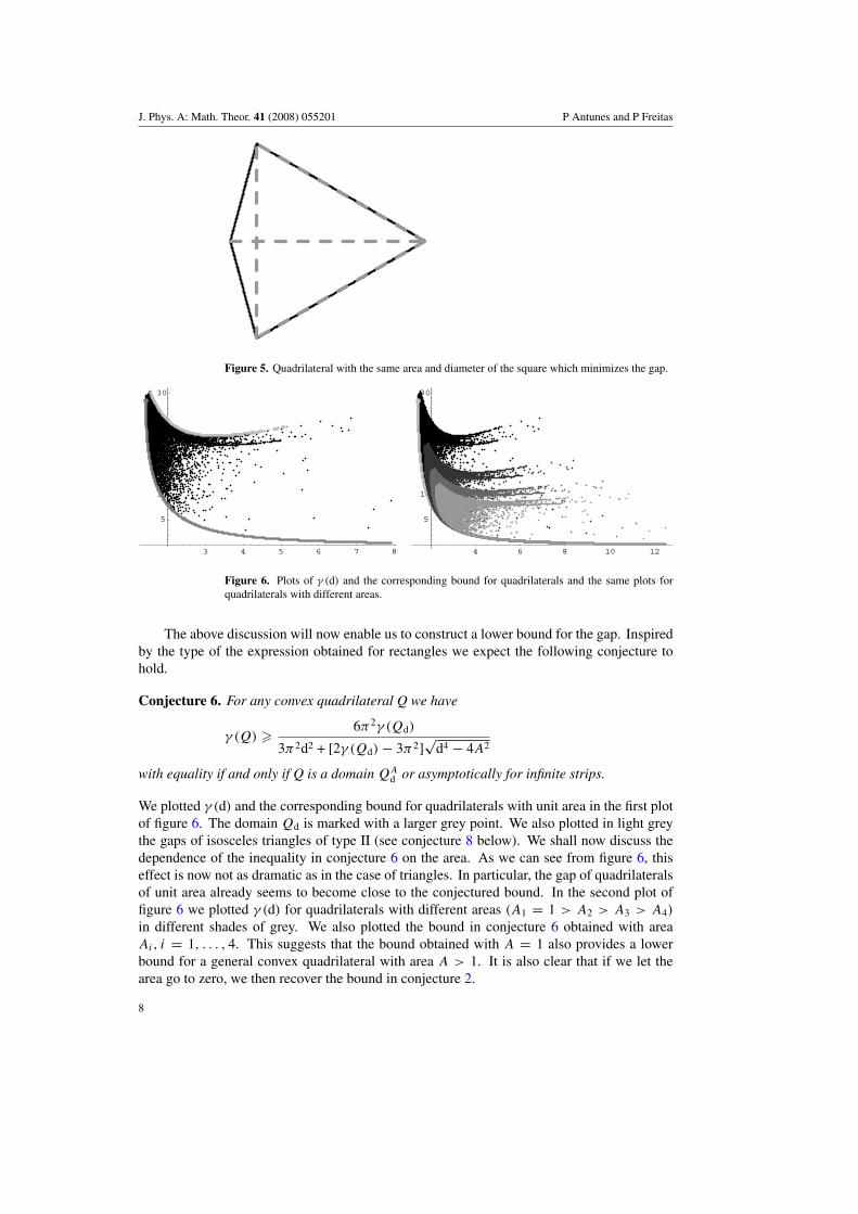
While the square does provide equality in the above inequality, it is not the only quadrilateralto do so. In fact, there is a continuous family of quadrilaterals in the same situation and whichwill thus play a role in what happens at the far end where the diameter is minimal. It is thusrelevant to study the gap for this family of domains. The numerical data gathered indicatesthat the square actually maximizes the gap, while the domain plotted in figure 5 minimizesit—all four lines marked with a dashed grey line have length equal to the diameter. In whatfollows we shall denote such quadrilaterals with area A by QA

d and in the case of unit area weshall simply write Qd.

7

J. Phys. A: Math. Theor. 41 (2008) 055201 P Antunes and P Freitas

Figure 5. Quadrilateral with the same area and diameter of the square which minimizes the gap.

3 4 5 6 7 8

5

10

15

20

25

30

4 6 8 10 12

5

10

15

20

25

30

Figure 6. Plots of γ (d) and the corresponding bound for quadrilaterals and the same plots forquadrilaterals with different areas.

The above discussion will now enable us to construct a lower bound for the gap. Inspiredby the type of the expression obtained for rectangles we expect the following conjecture tohold.

Conjecture 6. For any convex quadrilateral Q we have

γ (Q) � 6π2γ (Qd)

3π2d2 + [2γ (Qd) − 3π2]√

d4 − 4A2

with equality if and only if Q is a domain QAd or asymptotically for infinite strips.

We plotted γ (d) and the corresponding bound for quadrilaterals with unit area in the first plotof figure 6. The domain Qd is marked with a larger grey point. We also plotted in light greythe gaps of isosceles triangles of type II (see conjecture 8 below). We shall now discuss thedependence of the inequality in conjecture 6 on the area. As we can see from figure 6, thiseffect is now not as dramatic as in the case of triangles. In particular, the gap of quadrilateralsof unit area already seems to become close to the conjectured bound. In the second plot offigure 6 we plotted γ (d) for quadrilaterals with different areas (A1 = 1 > A2 > A3 > A4)

in different shades of grey. We also plotted the bound in conjecture 6 obtained with areaAi, i = 1, . . . , 4. This suggests that the bound obtained with A = 1 also provides a lowerbound for a general convex quadrilateral with area A > 1. It is also clear that if we let thearea go to zero, we then recover the bound in conjecture 2.

8

J. Phys. A: Math. Theor. 41 (2008) 055201 P Antunes and P Freitas

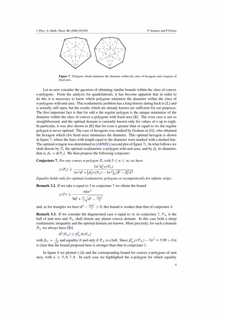
Figure 7. Polygons which minimize the diameter within the class of hexagons and octagons offixed area.

Let us now consider the question of obtaining similar bounds within the class of convexn-polygons. From the analysis for quadrilaterals, it has become apparent that in order todo this it is necessary to know which polygons minimize the diameter within the class ofn-polygons with unit area. This isodiametric problem has a long history dating back to [L] andis actually still open, but the results which are already known are sufficient for our purposes.The first important fact is that for odd n the regular polygon is the unique minimizer of thediameter within the class of convex n-polygons with fixed area [R]. The even case is not sostraightforward, and the optimal domain is currently known only for values of n up to eight.In particular, it was also shown in [R] that for even n greater than or equal to six the regularpolygon is never optimal. The case of hexagons was studied by Graham in [G], who obtainedthe hexagon which (for fixed area) minimizes the diameter. This optimal hexagon is shownin figure 7, where the lines with length equal to the diameter were marked with a dashed line.The optimal octagon was determined in [AHMX] (second plot of figure 7). In what follows weshall denote by Pn the optimal isodiametric n-polygon with unit area, and by βn its diameter,that is, βn = d(Pn). We then propose the following conjecure:

Conjecture 7. For any convex n-polygon Pn with 5 � n � ∞ we have

γ (Pn) � 3π2β2nγ (Pn)

3π2d2 +[β2

nγ (Pn) − 3π2]√

d4 − β4nA

2

Equality holds only for optimal isodiametric polygons or asymptotically for infinite strips.

Remark 3.2. If we take n equal to 3 in conjecture 7 we obtain the bound

γ (T ) � 64π2

9d2 + 373

√d4 − 16A2

3

and, as for triangles we have d4 − 16A2

3 � 0, this bound is weaker than that of conjecture 4.

Remark 3.3. If we consider the degenerated case n equal to ∞ in conjecture 7, P∞ is theball of unit area and P∞ shall denote any planar convex domain. In this case both a sharpisodiametric inequality and the optimal domain are known. More precisely, for such a domainP∞ we always have [Bi]

d2(P∞) � β2∞A(P∞)

with β∞ = 2√π

and equality if and only if P∞ is a ball. Since β2∞γ (P∞) − 3π2 ≈ 5.99 > 0 it

is clear that the bound proposed here is stronger than that in conjecture 2.

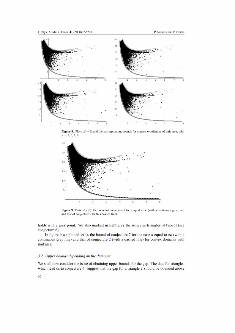
In figure 8 we plotted γ (d) and the corresponding bound for convex n-polygons of unitarea, with n = 5, 6, 7, 8. In each case we highlighted the n-polygon for which equality

9

J. Phys. A: Math. Theor. 41 (2008) 055201 P Antunes and P Freitas

3 4 5 6 7 8

5

10

15

20

25

30

2 3 4 5 6 7 8

5

10

15

20

25

30

2 3 4 5 6 7 8

5

10

15

20

25

30

2 3 4 5 6 7 8

5

10

15

20

25

30

Figure 8. Plots of γ (d) and the corresponding bounds for convex n-polygons of unit area, withn = 5, 6, 7, 8.

2 3 4 5 6 7 8

5

10

15

20

25

30

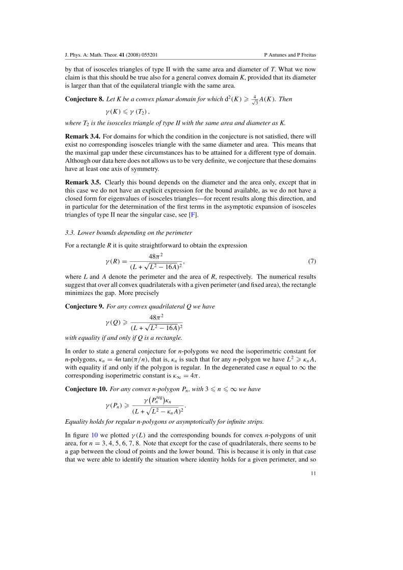
Figure 9. Plots of γ (d), the bound of conjecture 7 for n equal to ∞ (with a continuous grey line)and that of conjecture 2 (with a dashed line).

holds with a grey point. We also marked in light grey the isosceles triangles of type II (seeconjecture 8).

In figure 9 we plotted γ (d), the bound of conjecture 7 for the case n equal to ∞ (with acontinuous grey line) and that of conjecture 2 (with a dashed line) for convex domains withunit area.

3.2. Upper bounds depending on the diameter

We shall now consider the issue of obtaining upper bounds for the gap. The data for triangleswhich lead us to conjecture 4, suggest that the gap for a triangle T should be bounded above

10

J. Phys. A: Math. Theor. 41 (2008) 055201 P Antunes and P Freitas

by that of isosceles triangles of type II with the same area and diameter of T. What we nowclaim is that this should be true also for a general convex domain K, provided that its diameteris larger than that of the equilateral triangle with the same area.

Conjecture 8. Let K be a convex planar domain for which d2(K) � 4√3A(K). Then

γ (K) � γ (T2) ,

where T2 is the isosceles triangle of type II with the same area and diameter as K.

Remark 3.4. For domains for which the condition in the conjecture is not satisfied, there willexist no corresponding isosceles triangle with the same diameter and area. This means thatthe maximal gap under these circumstances has to be attained for a different type of domain.Although our data here does not allows us to be very definite, we conjecture that these domainshave at least one axis of symmetry.

Remark 3.5. Clearly this bound depends on the diameter and the area only, except that inthis case we do not have an explicit expression for the bound available, as we do not have aclosed form for eigenvalues of isosceles triangles—for recent results along this direction, andin particular for the determination of the first terms in the asymptotic expansion of isoscelestriangles of type II near the singular case, see [F].

3.3. Lower bounds depending on the perimeter

For a rectangle R it is quite straightforward to obtain the expression

γ (R) = 48π2

(L +√

L2 − 16A)2, (7)

where L and A denote the perimeter and the area of R, respectively. The numerical resultssuggest that over all convex quadrilaterals with a given perimeter (and fixed area), the rectangleminimizes the gap. More precisely

Conjecture 9. For any convex quadrilateral Q we have

γ (Q) � 48π2

(L +√

L2 − 16A)2

with equality if and only if Q is a rectangle.

In order to state a general conjecture for n-polygons we need the isoperimetric constant forn-polygons, κn = 4n tan(π/n), that is, κn is such that for any n-polygon we have L2 � κnA,with equality if and only if the polygon is regular. In the degenerated case n equal to ∞ thecorresponding isoperimetric constant is κ∞ = 4π .

Conjecture 10. For any convex n-polygon Pn, with 3 � n � ∞ we have

γ (Pn) �γ(P

regn

)κn

(L +√

L2 − κnA)2.

Equality holds for regular n-polygons or asymptotically for infinite strips.

In figure 10 we plotted γ (L) and the corresponding bounds for convex n-polygons of unitarea, for n = 3, 4, 5, 6, 7, 8. Note that except for the case of quadrilaterals, there seems to bea gap between the cloud of points and the lower bound. This is because it is only in that casethat we were able to identify the situation where identity holds for a given perimeter, and so

11

J. Phys. A: Math. Theor. 41 (2008) 055201 P Antunes and P Freitas

6 7 8 9 10 11 12

10

15

20

25

30

6 8 10 12 14 16

5

10

15

20

25

30

6 8 10 12 14 16

5

10

15

20

25

30

6 8 10 12 14 16

5

10

15

20

25

30

6 8 10 12 14 16

5

10

15

20

25

30

6 8 10 12 14 16

5

10

15

20

25

30

Figure 10. Plots of γ (L) and the corresponding bounds for convex n-polygons of unit area, withn = 3, 4, 5, 6, 7, 8.

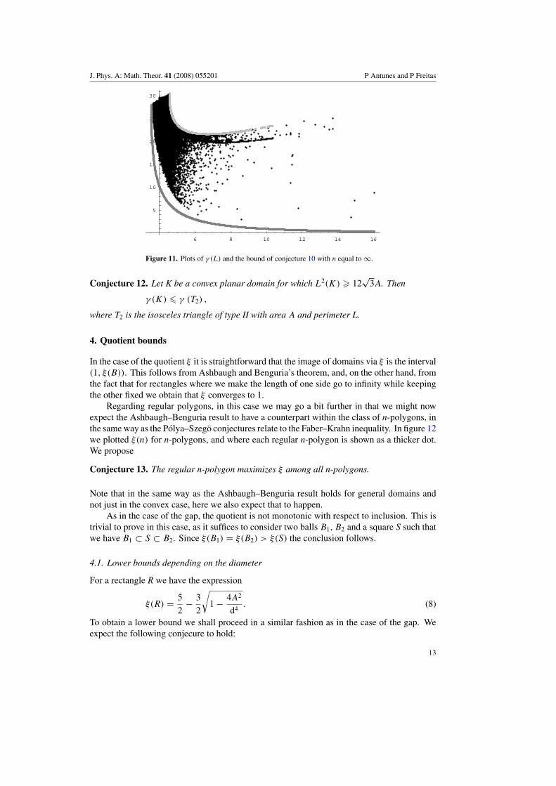
the bound is built from that example. Although infinite strips provide equality asymptotically,this will not be the case for rectangles when the perimeter is finite, if n is greater than four.In figure 11 we plotted γ (L) for n-polygons (3 � n � 8) for convex domains with unit areatogether with the bound of conjecture 10 with n equal to ∞, and where we plotted isoscelestriangles of type II in grey.

3.4. Upper bounds depending on the perimeter

As in the case of bounds depending on the diameter, we see that the gap is again bounded fromabove by that of isosceles triangles suggesting conjectures similar to conjectures 8 and 11. Inthe first plot of figure 10 we plotted γ (L) for triangles with unit area (the gaps for isoscelestriangles are plotted in light grey).

Conjecture 11. For any triangle T we have

γ (T1) � γ (T ) � γ (T2) ,

where T1 and T2 are (respectively) isosceles triangles of type I and type II with the same areaand perimeter as those of T.

12

J. Phys. A: Math. Theor. 41 (2008) 055201 P Antunes and P Freitas

6 8 10 12 14 16

5

10

15

20

25

30

Figure 11. Plots of γ (L) and the bound of conjecture 10 with n equal to ∞.

Conjecture 12. Let K be a convex planar domain for which L2(K) � 12√

3A. Then

γ (K) � γ (T2) ,

where T2 is the isosceles triangle of type II with area A and perimeter L.

4. Quotient bounds

In the case of the quotient ξ it is straightforward that the image of domains via ξ is the interval(1, ξ(B)). This follows from Ashbaugh and Benguria’s theorem, and, on the other hand, fromthe fact that for rectangles where we make the length of one side go to infinity while keepingthe other fixed we obtain that ξ converges to 1.

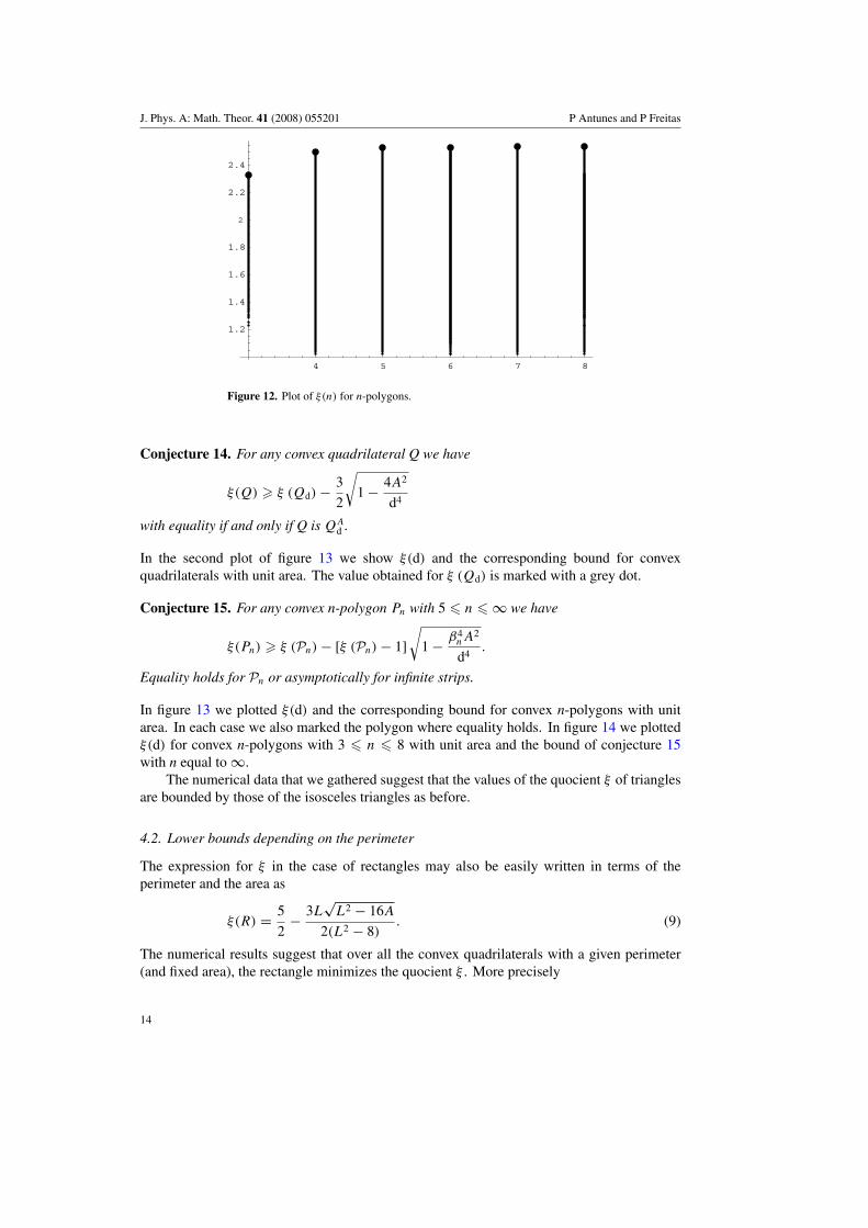
Regarding regular polygons, in this case we may go a bit further in that we might nowexpect the Ashbaugh–Benguria result to have a counterpart within the class of n-polygons, inthe same way as the Polya–Szego conjectures relate to the Faber–Krahn inequality. In figure 12we plotted ξ(n) for n-polygons, and where each regular n-polygon is shown as a thicker dot.We propose

Conjecture 13. The regular n-polygon maximizes ξ among all n-polygons.

Note that in the same way as the Ashbaugh–Benguria result holds for general domains andnot just in the convex case, here we also expect that to happen.

As in the case of the gap, the quotient is not monotonic with respect to inclusion. This istrivial to prove in this case, as it suffices to consider two balls B1, B2 and a square S such thatwe have B1 ⊂ S ⊂ B2. Since ξ(B1) = ξ(B2) > ξ(S) the conclusion follows.

4.1. Lower bounds depending on the diameter

For a rectangle R we have the expression

ξ(R) = 5

2− 3

2

√1 − 4A2

d4. (8)

To obtain a lower bound we shall proceed in a similar fashion as in the case of the gap. Weexpect the following conjecure to hold:

13

J. Phys. A: Math. Theor. 41 (2008) 055201 P Antunes and P Freitas

4 5 6 7 8

1.2

1.4

1.6

1.8

2

2.2

2.4

Figure 12. Plot of ξ(n) for n-polygons.

Conjecture 14. For any convex quadrilateral Q we have

ξ(Q) � ξ (Qd) − 3

2

√1 − 4A2

d4

with equality if and only if Q is QAd .

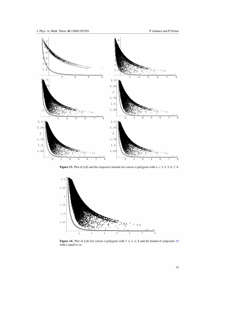
In the second plot of figure 13 we show ξ(d) and the corresponding bound for convexquadrilaterals with unit area. The value obtained for ξ (Qd) is marked with a grey dot.

Conjecture 15. For any convex n-polygon Pn with 5 � n � ∞ we have

ξ(Pn) � ξ (Pn) − [ξ (Pn) − 1]

√1 − β4

nA2

d4.

Equality holds for Pn or asymptotically for infinite strips.

In figure 13 we plotted ξ(d) and the corresponding bound for convex n-polygons with unitarea. In each case we also marked the polygon where equality holds. In figure 14 we plottedξ(d) for convex n-polygons with 3 � n � 8 with unit area and the bound of conjecture 15with n equal to ∞.

The numerical data that we gathered suggest that the values of the quocient ξ of trianglesare bounded by those of the isosceles triangles as before.

4.2. Lower bounds depending on the perimeter

The expression for ξ in the case of rectangles may also be easily written in terms of theperimeter and the area as

ξ(R) = 5

2− 3L

√L2 − 16A

2(L2 − 8). (9)

The numerical results suggest that over all the convex quadrilaterals with a given perimeter(and fixed area), the rectangle minimizes the quocient ξ . More precisely

14

J. Phys. A: Math. Theor. 41 (2008) 055201 P Antunes and P Freitas

3 4 5 6

1.2

1.4

1.6

1.8

2

2.2

3 4 5 6 7 8

1.2

1.4

1.6

1.8

2

2.2

2.4

3 4 5 6 7 8

1.25

1.5

1.75

2

2.25

2.5

2 3 4 5 6 7 8

1.25

1.5

1.75

2

2.25

2.5

2 3 4 5 6 7 8

1.25

1.5

1.75

2

2.25

2.5

2 3 4 5 6 7 8

1.25

1.5

1.75

2

2.25

2.5

Figure 13. Plot of ξ(d) and the respective bounds for convex n-polygons with n = 3, 4, 5, 6, 7, 8.

2 3 4 5 6 7 8

1.25

1.5

1.75

2

2.25

2.5

Figure 14. Plot of ξ(d) for convex n-polygons with 3 � n � 8 and the bound of conjecture 15with n equal to ∞.

15

J. Phys. A: Math. Theor. 41 (2008) 055201 P Antunes and P Freitas

6 7 8 9 10 11 12

1.2

1.4

1.6

1.8

2

2.2

6 8 10 12 14 16

1.2

1.4

1.6

1.8

2

2.2

2.4

6 8 10 12 14 16

1.25

1.5

1.75

2

2.25

2.5

6 8 10 12 14 16

1.25

1.5

1.75

2

2.25

2.5

6 8 10 12 14 16

1.25

1.5

1.75

2

2.25

2.5

6 8 10 12 14 16

1.25

1.5

1.75

2

2.25

2.5

Figure 15. Plot of ξ(L) and the respective bounds for n-polygons, with n = 3, 4, 5, 6, 7, 8.

Conjecture 16. For any convex quadrilateral Q we have

ξ(Q) � 5

2− 3L

√L2 − 16A

2(L2 − 8)

with equality if and only if Q is a rectangle.

Proceeding as before now yields

Conjecture 17. For a convex n-polygon Pn with 3 � n � ∞ we have

ξ(Pn) � ξ(P reg

n

) − 2[ξ(P

regn

) − 1]L

√L2 − κnA

2L2 − κnA.

Equality holds for regular n-polygons or asymptotically for infinite strips.

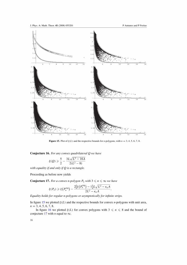
In figure 15 we plotted ξ(L) and the respective bounds for convex n-polygons with unit area,n = 3, 4, 5, 6, 7, 8.

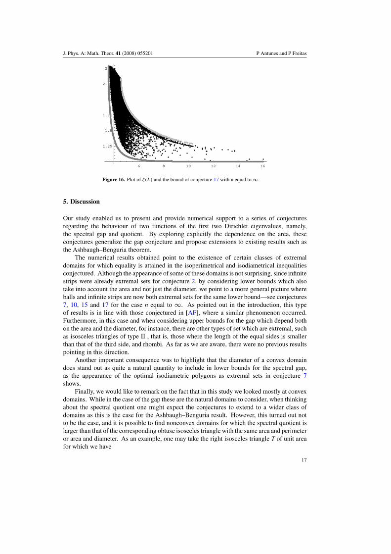
In figure 16 we plotted ξ(L) for convex polygons with 3 � n � 8 and the bound ofconjecture 17 with n equal to ∞.

16

J. Phys. A: Math. Theor. 41 (2008) 055201 P Antunes and P Freitas

6 8 10 12 14 16

1.25

1.5

1.75

2

2.25

2.5

Figure 16. Plot of ξ(L) and the bound of conjecture 17 with n equal to ∞.

5. Discussion

Our study enabled us to present and provide numerical support to a series of conjecturesregarding the behaviour of two functions of the first two Dirichlet eigenvalues, namely,the spectral gap and quotient. By exploring explicitly the dependence on the area, theseconjectures generalize the gap conjecture and propose extensions to existing results such asthe Ashbaugh–Benguria theorem.

The numerical results obtained point to the existence of certain classes of extremaldomains for which equality is attained in the isoperimetrical and isodiametrical inequalitiesconjectured. Although the appearance of some of these domains is not surprising, since infinitestrips were already extremal sets for conjecture 2, by considering lower bounds which alsotake into account the area and not just the diameter, we point to a more general picture whereballs and infinite strips are now both extremal sets for the same lower bound—see conjectures7, 10, 15 and 17 for the case n equal to ∞. As pointed out in the introduction, this typeof results is in line with those conjectured in [AF], where a similar phenomenon occurred.Furthermore, in this case and when considering upper bounds for the gap which depend bothon the area and the diameter, for instance, there are other types of set which are extremal, suchas isosceles triangles of type II , that is, those where the length of the equal sides is smallerthan that of the third side, and rhombi. As far as we are aware, there were no previous resultspointing in this direction.

Another important consequence was to highlight that the diameter of a convex domaindoes stand out as quite a natural quantity to include in lower bounds for the spectral gap,as the appearance of the optimal isodiametric polygons as extremal sets in conjecture 7shows.

Finally, we would like to remark on the fact that in this study we looked mostly at convexdomains. While in the case of the gap these are the natural domains to consider, when thinkingabout the spectral quotient one might expect the conjectures to extend to a wider class ofdomains as this is the case for the Ashbaugh–Benguria result. However, this turned out notto be the case, and it is possible to find nonconvex domains for which the spectral quotient islarger than that of the corresponding obtuse isosceles triangle with the same area and perimeteror area and diameter. As an example, one may take the right isosceles triangle T of unit areafor which we have

17

J. Phys. A: Math. Theor. 41 (2008) 055201 P Antunes and P Freitas

γ (T ) = 5π2

2≈ 24.674 ξ(T ) = 2.

The quadrilateral Q with vertices at (−a, 0), (0, b), (a, 0) and (0, b + c) with a = 1/c = 9/10and

b = −5

9+

1

5

(483 033 + 144 875

√2

640 78

)(1/2)

≈ 0.0998,

has the same area and perimeter as the right isosceles triangle considered. However,γ (Q) ≈ 32.09 and ξ(Q) ≈ 2.114. If one takes instead the quadrilateral Q′ with verticesat (−√

2, 0), (0.1, 0), (−0.05, 1/√

2) and (0,√

2) we have that Q′ has the same area anddiameter as T but now γ (Q) ≈ 26.62 and ξ(Q) ≈ 2.070.

Although it is our belief that many of the conjectures presented here are probably beyondcurrent available analytical techniques, we hope that this study will contribute to a betterunderstanding of the behaviour of the two quantities involved, and, at a more general level, ofthe relations between eigenvalues and geometrical quantities such as those considered here.

Acknowledgments

Partially supported by FCT, Portugal, through programs POCTI/MAT/60863/2004 andPOCTI/POCI2010.

References

[AA] Alves Carlos J S and Antunes Pedro R S 2005 The method of fundamental solutions applied to thecalculation of eigenfrequencies and eigenmodes of 2D simply connected shapes, Computers Comput.Mater. Continua 2 251–66

[AF] Antunes P and Freitas P 2006 New bounds for the principal Dirichlet eigenvalue of planar regions Exp.Math. 15 333–42

[A] Ashbaugh M 2006 The fundamental gap, AIM 2006, available electronically at http://www.aimath.org/WWN/loweigenvalues/gap.pdf

[AB] Ashbaugh M and Benguria R 1992 A sharp bound for the ratio of the first two eigenvalues of the DiricheltLaplacian and extensions Ann. Math. 135 601–28

[AHMX] Audet C, Hansen P, Messine F and Xiong J 2002 The largest small octagon J. Comb. Theory A 98 46–59[BK] Banuelos R and Kroger P 2001 Gradient estimates for the ground-state Schrodinger eigenfunction and

applications Comm. Math. Phys. 224 545–50[Be] Berg M van den 1983 On condensation in the free-boson gas and the spectrum of the Laplacian J. Stat.

Phys. 31 623–37[Bi] Bieberbach A 1915 Ubber eine Extremaleigenschaft des Kreises Jber. Deutsch. Math.-Vereinig 24 247–50

[BF] Borisov D and Freitas P 2007 Singular asymptotic expansions for Dirichlet eigenvalues and eigenfunctionson thin planar domains Ann. Inst. H. Poincare Anal Non Lineaire at press

[BZ] Burago Yu D and Zalgaller V A 1988 Geometric Inequalities (Berlin: Springer)[D] Davis B 2001 On the spectral gap for fixed membranes Ark. Mat. 39 65–74

[EF] Elbert A and Laforgia A 1998 Asymptotic expansion for zeros of Bessel functions and their derivatives forlarge order Att. Sem. Mat. Fis. Univ. Modena XLVI 685–95

[F] Freitas P 2007 Precise bounds and asymptotics for the first Dirichlet eigenvalue of rhombi and isoscelestriangles J. Funct. Anal. doi:101016/jfa.2007.04.012

[FK] Freitas P and Krejcirık D A sharp upper bound for the first Dirichlet eigenvalue and the growth of theisoperimetric constant of convex domains Proc. Am. Math. Soc. at press

[G] Graham R L 1975 The largest small hexagon J. Comb. Theory A 18 165–70[L] Lens H 1956 Ungeloste Probleme: Nr. 12 Elem. Math. 11 86

[LY] Levitin M and Yagudin R 2003 Range of the first three eigenvalues of the planar Dirichlet Laplacian LMSJ. Comput. Math. 6 1–17

[M] Melas A 1992 The stability of some eigenvalue estimates J. Differ. Geom. 36 19–33

18

J. Phys. A: Math. Theor. 41 (2008) 055201 P Antunes and P Freitas

[PPW] Payne L E, Polya G and Weinberger H F 1956 On the ratio of consecutive eigenvalues J. Math. Phys. 35289–98

[PW] Payne L E and Weinberger H F 1961 Some isoperimetric inequalities for membrane frequencies andtorsional rigidity J. Math. Anal. Appl. 2 210–6

[R] Reinhardt K 1922 Extremale Polygone gegebene Durchmessers Jber. Deutsch. Math.-Verein. 31 251–70[SWYY] Singer I M, Wong B, Yau S-T and Yau S S-T 1985 An estimate of the gap of the first two eigenvalues in

the Schrodinger operator Ann. Scuola Norm. Sup. Pisa Cl. Sci. 12 319–33[Si] Siudeja B 2007 Isoperimetric inequalities for eigenvalues of triangles Preprint

[Sm] Smits R 1996 Spectral gaps and rates to equilibrium in convex domains Michigan Math. J. 43 141–57[TB] Trefethen L N and Betcke T 2006 Computed eigenmodes of planar regions Recent Advances in

Differential Equations and Mathematical Physics (Contemp. Math. vol 412) (Providence, RI: AmericanMathematical Society) pp 297–314

[YZ] Yu Q and Zhong J Q 1986 Lower bounds for the gap between the first and second eigenvalues of theSchrodinger operator Trans. Am. Math. Soc. 294 341–9

19