IEEE TRANSACTIONS ON GEOSCIENCE AND REMOTE SENSING, VOL. 49, NO. 8, AUGUST 2011 2887

A Novel Two-Way Finite-Element ParabolicEquation Groundwave Propagation Tool: Tests

With Canonical Structures and CalibrationGökhan Apaydin, Senior Member, IEEE, Ozlem Ozgun, Member, IEEE,

Mustafa Kuzuoglu, Member, IEEE, and Levent Sevgi, Fellow, IEEE

Abstract—A novel two-way finite-element parabolic equation(PE) (2W-FEMPE) propagation model which handles both for-ward and backward scattering effects of the groundwave propaga-tion above the Earth’s surface over irregular terrain paths throughinhomogeneous atmosphere is introduced. A Matlab-based propa-gation tool for 2W-FEMPE is developed and tested against math-ematical exact and asymptotic solutions as well as the recentlyintroduced two-way split-step PE model through a canonical val-idation, verification, and calibration process for the first time inliterature.

Index Terms—Atmospheric refractivity, Claerbout equation,ducting, electromagnetic (EM) propagation, fast Fourier trans-form (FFT), finite-element method (FEM), Matlab, narrow angle,split-step parabolic equation (PE) (SSPE), terrain effect, waveequation, wide angle.

I. INTRODUCTION

ONE of the principal goals of a propagation engineer isto develop an effective numerical propagation tool that

accurately calculates the path loss between any two pointsspecified on a digital map of the area of interest. The accuratemodeling of the groundwave propagation over the Earth’s sur-face is usually a challenging task because of several complexprocesses occurring during the propagation. In particular, theterrain irregularities reflect and diffract energy in a compli-cated way and have a significant impact on the radiowavepath loss. Such terrain effects become even more pronouncedwhen coupled with atmospheric refraction because an inhomo-geneous atmosphere may redirect energy and cause multipleinteractions with the ground. This, in turn, certainly requires

Manuscript received June 9, 2010; revised September 30, 2010 andDecember 22, 2010; accepted February 6, 2011. Date of publicationMarch 24, 2011; date of current version July 22, 2011.

G. Apaydin is with the Department of Electrical and Electronics Engi-neering, Zirve University, 27260 Gaziantep, Turkey (e-mail: gokhan.apaydin@zirve.edu.tr).

O. Ozgun is with the Department of Electrical and Electronics Engineer-ing, Middle East Technical University, Northern Cyprus Campus, Guzelyurt,10 Mersin, Turkey (e-mail: ozozgun@metu.edu.tr).

M. Kuzuoglu is with the Department of Electrical and Electronics Engi-neering, Middle East Technical University, 06531 Ankara, Turkey (e-mail:kuzuoglu@metu.edu.tr).

L. Sevgi is with the Department of Electronics and CommunicationsEngineering, Dogus University, 34722 Istanbul, Turkey (e-mail: lsevgi@dogus.edu.tr).

Color versions of one or more of the figures in this paper are available onlineat http://ieeexplore.ieee.org.

Digital Object Identifier 10.1109/TGRS.2011.2114889

a good understanding of electromagnetic (EM) wave behav-ior in the presence of irregular terrain and inhomogeneousatmosphere. Therefore, a generally applicable all-purpose prop-agation prediction method/tool must be able to predict theeffect of such complex environmental factors/uncertainties onthe performance of radio communication and radar systems[1]. However, since the complexity of the realistic propagationscenarios may place limitations in the range of validity ofthe prediction models/tools, the fidelity of the models to theunderlying physics must be assessed by means of, for example,validation, verification, and calibration (VV&C) tests. Thisprocess of determining whether the right model is built (orsolving the right equations) is called “validation,” whereasthe “verification” assessment examines if the model is builtright. The final step is the “calibration,” which is the processof quantitatively defining the performance of the model withrespect to known and controlled models (such as exact solutionsand/or other numerical methods).

In the past, various methods/tools have been developed forpredicting EM wave propagation in the atmosphere, such asgeometric optics, physical optics, and normal mode analysis.However, the presence of a vertical refractivity profile in theatmosphere complicates the application of some of these meth-ods. In geometric optics (or ray theory), the difficulties asso-ciated with the focusing and identification of rays render themethod inconvenient for modeling reflection/diffraction effectsin nonstandard atmospheres. The mode theory can be employedfor ducting environments but becomes intractable when com-plex refractive structures are involved. The cost of compu-tation in modal analysis might place limitations in obtainingconvergent solutions, even in the case of simple refractivityprofiles. Thus, it is not feasible to apply these methods, evenhybrid combinations of them, to inhomogeneous atmospheresof range-dependent problems.

The one-way parabolic equation (PE) method has been oneof the widely used propagation tools to model the ground-wave propagation over the 2-D Earth’s surface because of itsflexibility in modeling both horizontally and vertically varyingatmospheric refraction effects and irregular terrain paths [1]–[17]. The standard parabolic wave equation (PWE) is derivedfrom Helmholtz’s equation by eliminating the rapidly vary-ing phase term to obtain a reduced function that has a slowvariation in range for propagating angles close to the paraxialdirection. Helmholtz’s equation is approximated in terms of two

0196-2892/$26.00 © 2011 IEEE

2888 IEEE TRANSACTIONS ON GEOSCIENCE AND REMOTE SENSING, VOL. 49, NO. 8, AUGUST 2011

differential equations, both of which are in PWE form, belong-ing to forward and backward propagating waves. In the standardPE method, only the PWE corresponding to the forward partis solved, which makes the method a one-way forward-scattermodel. The standard PE method has been first introduced byLeontovich and Fock [2]. However, the development of theFourier split-step algorithm by Hardin and Tappert [3] hasinitiated the wide-spread usage of the method in various prop-agation scenarios. Generally speaking, the Fourier split-stepPE (SSPE) algorithm is a marching-type initial-value problem,which computes an initial field from a known antenna patternlocated at a reference range and determines the field alongthe vertical direction at each range step by using the fieldat the preceding range step through the utilization of Fouriertransformations between transverse spatial and wavenumberdomains.

The step-by-step solution of the standard PWE has alsobeen achieved by employing finite-difference methods [8]–[11]and finite-element methods (FEMs) [18]–[22] along each verti-cal direction. Although the SSPE algorithm is a more robustand faster algorithm and can handle larger range increments(in terms of wavelength), the major advantage of the finitemethods, over the SSPE, is the easiness in handling arbitraryboundary conditions (BCs). In particular, the FEM has beenwidely used in the EM modeling due to its adaptability toarbitrary geometries and material inhomogeneities. Therefore,to make a compromise, the finite methods can be preferred incomplex propagation environments involving different surfaceimpedances [20]–[22].

The standard PWE is a narrow-angle approximation andrestricts the accuracy to propagation angles up to 10◦–15◦

from the paraxial direction [9]. Usually, this is not a seriousrestriction since most of the long-range propagation scenariosencounter propagation angles that are usually less than a fewdegrees. On the other hand, short-range propagation problemsas well as the problems involving multiple reflections anddiffractions because of hills and valleys with steep slopes ne-cessitate models that are effective for larger propagation angles.Wide-angle PE propagators have been introduced to handlepropagation angles up to 40◦–45◦ [11], [23]–[26].

All of the aforementioned approaches offer one-way prop-agation modeling and neglect the backward propagation andmultipath effects. Ignoring backward waves may not be seriousfor long-range propagation problems, where the energy carriedby the forward propagating waves dominates. However, obsta-cles and/or irregular terrain along the propagation path neces-sitate the well prediction of the backward reflected, refracted,and diffracted waves to achieve reliable results. The two-wayversions of the SSPE algorithm have also been introduced fordifferent applications and with implementation schemes [9],[27]–[38]; pioneer works have been studied in [27] and [28]on the construction of analytical solutions to the integral andfunctional equations based on two-way PE (2W-PE) providingthe exact solution for the current on a perfectly conducting strip(refer to [29]–[31] for details), in acoustic wave propagation inelastic media [32], then in multiple scattering modeling [33],in multiple diffraction modeling [34], and in multiple knife-edge modeling [35]. The underlying idea, in all these, is switch-

ing the direction of propagation in the standard PE methodin a forward–backward manner. Recently, a two-way SSPE(2W-SSPE) has been proposed to account for multiple-reflection effects over arbitrary staircase-approximated irregu-lar terrain profiles [36] and then calibrated by means of varioussystematic tests and comparisons [37], [38]. In this paper, thetwo-way finite-element PE (2W-FEMPE) propagation tool ispresented and calibrated in certain canonical and/or complexscenarios for the first time in literature. The VV&C of the2W-FEMPE model is performed against the analytical data, theImage Method and the Geometric Optic (GO) + AsymptoticTheory of Diffraction [39]–[41], as well as the recently pro-posed 2W-SSPE model [36]–[38]. Narrow- and wide-angle PEmodels are also discussed here, for the sake of completeness.It is generally accepted that the simplest conceptual radiowavepropagation model is GO. The EM field is locally a plane wavein a medium that changes slowly, and wave energy propagatesalong rays that are perpendicular to the wavefronts. Snell’slaw can be applied repeatedly to find out ray trajectories inthis medium. Unfortunately, GO fails near caustics and it alsoignores the effects of diffraction. The PE model is based onparabolic approximation of the wave equation which admitsa very feasible numerical marching solution. The PE modelcontains information missing in the GO model such as thebehavior near caustics and shadow boundaries. Also, the PEmodel is frequency dependent, but GO is frequency indepen-dent. The GO needs precise calculation of optical ray paths andcoherent integration of the family of rays passing through thesame observation point.

This paper is organized as follows: Section II summarizesthe standard one-way PE method and its implementation viathe Fourier SSPE algorithm. Section III introduces the deriva-tions of the FEMPE model together with the two-way algo-rithm. Canonical tests, comparisons, and calibration results aredemonstrated in Section IV. Finally, Section V draws someconclusions.

Throughout this paper, the suppressed time dependence ofthe form exp(−iωt) is assumed.

II. PE MODEL

The scalar wave function ψ(x, z) can be obtained as thesolution of the following 2-D Helmholtz equation:

{∂2

∂x2+

∂2

∂z2+ k20n

2(x, z)

}ψ(x, z) = 0 (1)

subject to given BCs. Here, n(x, z) is the refractive index,k0 = 2π/λ is the free space wavenumber (λ is the wave-length), and z and x stand for the transverse (height aboveground) and longitudinal (range) coordinates, respectively. Fur-thermore, ψ(x, z) corresponds to either electric or magneticfield components for horizontal and vertical polarizations. Notethat some researchers use the terms perpendicular and parallelpolarizations, whereas others prefer horizontal or vertical polar-izations. Here, we assume an xz plane as the 2-D environment.The TM (vertical polarization) and TE (horizontal polarization)equations use (Ex, Hy, Ez) and (Hx, Ey, Hz), respectively

APAYDIN et al.: TWO-WAY FINITE-ELEMENT PARABOLIC EQUATION GROUNDWAVE PROPAGATION TOOL 2889

Fig. 1. 2W-PE propagation model with (right arrows) forward and (leftarrows) backward propagating waves generated from terrain reflections.

[42]. Therefore, ψ(x, z) is the Hy and Ey for TM and TEpolarizations, respectively. Considering that the direction ofwave propagation is predominantly along the +x-axis paraxialdirection, the PWE is written by separating rapidly varyingphase terms (ψ(x, z) = exp(ik0x)u(x, z)). That is, the PWEin terms of the slowly varying amplitude function u(x, z) isexpressed as follows:{

∂

∂x+ ik0(1−Q)

}{∂

∂x+ ik0(1 +Q)

}u(x, z) = 0 (2)

where Q = (1 + q)1/2 and q = k−20 ∂2/∂z2 + (n2 − 1) if the

refractive index is independent of range.1 The first and sec-ond parts of (2) correspond to the forward and backwardpropagating waves, respectively (see Fig. 1). If the backwardpropagation is ignored, (2) reduces to{

A0∂

∂x+A1

∂3

∂z2∂x+A2 +A3

∂2

∂z2

}u(x, z) = 0 (3)

with the help of (1 + q)1/2 ≈ (a0 + a1q)/(b0 + b1q) approx-imation; therefore, A0 = b0 + b1(n

2 − 1), A1 = b1k−20 , A2 =

ik0((b0 − a0) + (b1 − a1)(n2 − 1)), and A3 = ik−1

0 (b1 − a1).If the angle of propagation measured from paraxial direction

is less than 15◦, the standard PE is obtained with the helpof square root approximation (

√1+q ≈ 1+q/2); therefore,

A0=1, A1=0, A2=−0.5ik0(n2 − 1), and A3=−0.5ik−1

0 .If the propagation angle is more than 15◦, the Claerboutequation is obtained by using the first-order Padé approxi-mation (

√1+q ≈ (1+0.75q)/(1+0.25q)); therefore, A0=1+

0.25(n2−1), A1=0.25k−20 , A2=−0.5ik0(n

2−1), and A3=−0.5ik−1

0 to satisfy the propagation angles up to 40◦ [37].The standard fast Fourier transform (FFT)-based SSPE so-

lution for the narrow and wide angles, respectively, are shownin [9], [23]–[26]

u(x+Δx, z)

=exp[0.5ik0(n

2 − 1)Δx]

×F−1{exp

[−(ik2zΔx

)/(2k0)

]F {u(x, z)}

}(4)

u(x+Δx, z)

=exp [ik0(n−1)Δx]

×F−1

{exp

[−(ik2zΔx

)/

(k0

(1+

√1−k2z/k

20

))]

× F {u(x, z)}} (5)

1This assumption does not violate the applicability of PWE to range-dependent refractivity profiles, because it is valid for each range step duringthe split-step solution of PWE, which will be clear in the sequel.

where F refers to the Fourier transform and kz is the transformvariable (i.e., transverse wavenumber). These equations areamenable to obtain the vertical field u(x+Δx, z) along xat each range step of Δx. Hence, the FFT-based PE solutionemploys a longitudinally marching procedure. First, an an-tenna pattern representing the initial height profile is injected.Next, this initial field is propagated longitudinally from x0 tox0 +Δx, and the transverse field profile at the next range isobtained. This new height profile is then used as the initialprofile for the next step, and the procedure is repeated untilthe propagator reaches the desired range. It is worthwhileto note that the effects of the Earth’s curvature are includedin the PE model via n → n+ z/ae where ae is the Earth’sradius.

The appropriate transverse BC over the flat-Earth’s surface isgiven as

{∂

∂z+ α

}u(x, z)

∣∣∣∣z=0

= 0. (6)

In general, a Cauchy-type impedance BC (i.e., lossy Earth’ssurface), which is introduced via α = ik0

√γ − 1 and α =

ik0√γ − 1/γ for horizontal and vertical polarizations, respec-

tively. Here, γ = εr + i60σλ is computed in terms of the con-ductivity (σ) and relative permittivity (εr) of the ground [43].For the perfect electric conductor (PEC) surface, Dirichlet andNeumann BCs (DBC and NBC) have been taken into considera-tion for horizontal and vertical polarizations, respectively. In theFFT-based SSPE algorithm, to satisfy the BCs over the Earth’ssurface, the surface is removed by taking a mirror copy of theinitial vertical field profile with respect to the surface (odd/evensymmetric for DBC/NBC, respectively). Another choice isto use one-sided sine/cosine transforms (sinFFT/cosFFT) forDBC/NBC, respectively. Since the propagation problem in-volves a physical domain extending vertically to infinity, anabrupt truncation is required at certain height, and therefore,the upper BC must be satisfied to avoid nonphysical reflections.Such artificial reflections can be obviated by introducing ab-sorbing layers above the height of interest [9].

III. FEMPE PROPAGATION TOOL

A. 1W-FEMPE Model

The initial phase of the FEM-based PWE procedure is todivide the transverse domain between the ground and the user-defined maximum height (Zmax) into a number of elements.Next, starting from the initial field at x = 0, the approximatedfield values at the selected discrete nodes in the vertical domainare propagated longitudinally by applying the Crank–Nicholsonapproach, which is based on the improved Euler method [44]–[46]. Although the Crank–Nicholson technique is inherentlyfast, it requires that both height and range step sizes, namely,Δz and Δx, respectively, should be chosen as small as nec-essary to overcome numerical oscillation problems, which ob-viously decelerate the speed of the method (refer to [22] fordetailed discussions).

2890 IEEE TRANSACTIONS ON GEOSCIENCE AND REMOTE SENSING, VOL. 49, NO. 8, AUGUST 2011

To formulate the one-way FEMPE (1W-FEMPE), we startwith (3) whose coefficients are chosen by considering narrow-and wide-angle approximations. Note that some coefficients arefunctions of z because of the refractivity index n. However,the coefficients are assumed to be constant for each element byfinding the value of the refractive index at the midpoint of eachelement. By multiplying (3) by a smooth test function v(z) withthe given BC in (6) and by using the integration-by-parts rule,one obtains

Zmax∫0

[∂

∂x

(A0u(x, z)v(z)−A1

∂u(x, z)

∂z

∂v(z)

∂z

)

+ A2u(x, z)v(z)−A3∂u(x, z)

∂z

∂v(z)

∂z

]dz

+A1∂

∂x

(∂u(Zmax)

∂zv(Zmax)−

∂u(0)

∂zv(0)

)

+A3

(∂u(Zmax)

∂zv(Zmax)−

∂u(0)

∂zv(0)

)= 0. (7)

The last two terms of (7) should be taken into considerationaccording to BCs. Replacing u(x, z) with the approximatedsolution

uap(x, z) =

ne∑e=1

2∑j=1

cej(x)Bej (z) (8)

where ne is the number of elements and cej(x) indicates thecoefficients of the unknown function. Moreover, the basisfunctions are chosen as the linear piecewise Lagrange poly-nomials as follows: Be

1(z) = (ze2 − z)/(ze2 − ze1) and Be2(z) =

(z − ze1)/(ze2 − ze1), where e stands for the element between

nodes ze1 and ze2. By choosing the test function v(z) as the sameas the basis function Bm(z) for m = 1, 2, the matrix form of(7) is

A∂c

∂x+Bc = 0 (9)

with A = A0M−A1K and B = A2M−A3K+A3BCor (A0M

emj − A1K

emj){∂cej/∂x} + (A2M

emj − A3K

emj +

A3BCemj){cej} = {0} for e = 1, . . . , ne, m = 1, 2, and

j = 1, 2 with

Memj =

ze2∫

ze1

BemBe

j dz Kemj =

ze2∫

ze1

∂Bem

∂z

∂Bej

∂zdz (10)

and BCemj is taken into consideration with BCs as BC1

11 =α for each step in x, x+Δx, . . .. The ground properties areincorporated into the FEM with the help of the matrix BC.The elemental matrices between nodes ze1 and ze2 for the linearpiecewise Lagrange polynomials are obtained as

[Me] =Δz

6

[2 11 2

][Ke] =

1

Δz

[1 −1−1 1

]. (11)

Using Crank–Nicholson approximation based on the im-proved Euler method for k = 2, . . . , Nx where Nx is the num-ber of nodes in the horizontal domain, the new coefficients forthe next step are obtained as

(A+B

Δx

2

)ck =

(A−B

Δx

2

)ck−1 (12)

which yields an unconditionally stable system and accu-rate method with the discretization error O(Δx2). The co-efficients of the initial field c1 at x = 0 can be generatedfrom the Gaussian antenna pattern specified by its height(hv), 3-dB beamwidth angle (θbw), and tilt angle (θtilt).Although Crank–Nicholson provides a fast solution, it hassome disadvantages since oscillation occurs for large Δx[22], [45].

B. 2W-FEMPE Model

The 2W-FEMPE approach is the iterative implementationof the 1W-FEMPE algorithm by simply rotating the directionof propagation in a forward–backward manner to estimatethe multiple-reflection effects. The principle idea is based onthe 2W-SSPE proposed in [32]–[34]. The algorithm can beapplied to a variable terrain by using staircase approximations,as shown in Fig. 1. If the vertical field meets a verticalterrain facet, it is split into two components propagatingin forward and backward directions. The forward fieldcontinues in the usual way after setting it to zero on thevertical terrain facet. In other words, the fields (at x+Δx)obtained from the previous vertical field (at x) are set to zeroinside the terrain (between z = 0 and z = zter(x0 +Δx)).However, it is evident that the field must be partiallyreflected from the terrain facet. Therefore, first the initialfield of the backward field is obtained by imposing theBCs at the facet (i.e., the tangential field must be zero onthe PEC facet), and then, this initial field is marched backin the −x direction by reversing the signs of k0 and Δx.Namely, the backward propagating waves are initiated fromthe waves between z = zter(x) and z = zter(x0 +Δx)and then propagated in the reverse direction. Note thatthe same form of the PWE is derived, as expected,for the reduced function in the backward propagation,but the original field is expressed as ψb(x, z) =ub(x, z) exp(−ik0x).

Both forward and backward fields continue to march out intheir own propagation directions. At each time the wave hits aterrain facet, it is again split into forward and backward com-ponents. The total field inside the domain is then determinedby the superposition of the backward and forward fields ateach range step. It is useful to note that the convergence ofthe algorithm is achieved because, as the iterations are carriedout, the field contributions of the multiple reflections decreasewith regard to the 1/

√r term in the 2-D Green’s function.

The convergence of the algorithm is checked against a certainthreshold criterion, which compares the total fields at eachiteration.

APAYDIN et al.: TWO-WAY FINITE-ELEMENT PARABOLIC EQUATION GROUNDWAVE PROPAGATION TOOL 2891

IV. CANONICAL TESTS, COMPARISONS,AND CALIBRATION

A. Tests With 1W-FEMPE Model

In this section, both 1W- and 2W-FEMPE algorithms arecalibrated through some canonical tests and comparisons. Acritical issue in these calibrations is the construction of thereference (analytical exact/approximate) solution [47]. First,2-D propagation inside a parallel-plate waveguide with PECboundaries is taken into account. The horizontally polarizedwave function inside a PEC parallel-plate waveguide with widthd under DBC, which is located longitudinally along x, may berepresented in terms of modal summation given as

u(x, z) =2

d

N∑q=1

cq sin(qπ

dz)exp(iβqx) (13)

where N is the total number of modes, βq =√

k20 − (qπ/d)2

is the longitudinal propagation constant for the mode q, and cqis the modal excitation coefficient numerically derived from thevertical orthonormality condition as

cq =

d∫0

g(z) sin(qπ

dz)dz. (14)

Here, g(z) = (2πσ2)−1/2 exp[(z − hv)2/(2σ2)] and σ is the

spatial width of the Gaussian source. The Gaussian sourcepattern is often used in applications since it represents variousantenna types. The Gaussian antenna pattern can also be definedin the vertical wavenumber domain as

g(kz) = exp

[−k2z ln2

2k20 sin2(θbw/2)

]. (15)

The tilt (or elevation) angle θtilt is introduced by shifting theantenna pattern, i.e., g(kz) → g(kz − k0 sin θtilt). The verticalfield distribution in the spatial domain is then obtained bytaking the inverse Fourier transform of (15).

The limiting case for the source function u(x, z) is theline-source representation which requires an infinite numberof modes (N → ∞) in the modal summation. The numberof modes would be finite for any other source function. It iscommon to choose a vertically extending Gaussian functionwith arbitrary location having vertical tilt angle in the range of±90◦. Note that the modal excitation coefficient cq is real fora real source function without any tilt and becomes complex ifthere is a downward/upward tilt no matter if the source functionis real or not. The number of modes, which are necessary forthe modal summation representation for a vertical Gaussiansource function located at midheight of an 8-m-wide parallel-plate waveguide, is listed in Table I. As observed, the numberof modes is less than a few hundreds even for ±45◦ verticaltilts. The higher the tilt angles (or frequency), the higher thenumber of modes required in the modal summation. Moreover,the number of modes increases as the vertical source beamwidthgets narrower.

Assuming a horizontally polarized Gaussian source at 1 GHzwith 3-dB beamwidth of 7◦, located at midheight and tilted 30◦

TABLE IPARALLEL-PLATE PEC WAVEGUIDE: NUMBER OF MODES (N) AS A

FUNCTION OF MAXIMUM INITIAL FIELD ERRORS AND VARIOUS TILT

ANGLES AT 1 GHZ. (A) θbw = 35◦. (B) θbw = 7◦ [hv = 4 m, d = 8 m]

Fig. 2. Parallel-plate PEC waveguide modeled with narrow-angle propagator.(Top) FEMPE (Δz = 5 mm and Δx = 17 mm). (Bottom) SSPE (Δz =20 mm and Δx = 67 mm) with −30◦ tilted waves at 1 GHz (hv = 4 m,θbw = 7◦, and d = 8 m).

downward, inside an 8-m-wide parallel-plate PEC waveguideunder DBC, the performances of narrow- and wide-angle PEtools with respect to the analytical result are shown in Figs. 2and 3 by means of 3-D field maps. The two field maps inFig. 2 alone (generated with the narrow-angle 1W-FEMPE and1W-SSPE tools) seem to be logical and physical. A down-tilted Gaussian beam is bouncing up and down while lon-gitudinally propagating with the interference patterns exactlylike that shown in the figure. On the other hand, the true 3-Dwave patterns are shown in Fig. 3. The analytical exact so-lution is exactly the same as the FEMPE and SSPE resultsof Fig. 3 and is not shown here. Hence, these results validatethe accuracy of the wide-angle FEMPE and SSPE and showthat the narrow-angle FEMPE and SSPE cannot handle largetilt angles. To validate the narrow-angle model, the angle mustbe constrained to be less than 10◦–15◦ while considering bothbeamwidth and tilt angles. Figs. 4 and 5 show horizontal fieldprofiles computed via analytical, FEMPE, and SSPE modelsat two different heights. In Fig. 4, the results computed vianarrow-angle FEMPE and SSPE tools are compared against

2892 IEEE TRANSACTIONS ON GEOSCIENCE AND REMOTE SENSING, VOL. 49, NO. 8, AUGUST 2011

Fig. 3. Parallel-plate PEC waveguide modeled with wide-angle propagator.(Top) FEMPE. (Bottom) SSPE with the same parameters as in Fig. 2.

Fig. 4. Parallel-plate PEC waveguide (narrow case). Horizontal field profilesat two different heights with the same parameters as in Fig. 2.

the reference solution. As observed, FEMPE and SSPE agreevery well but they both disagree with the reference (analytical)solution. This is an interesting example since it shows thatboth FEMPE and SSPE pass the verification test but fail fromthe (model) validity test. The same comparison computed viathe wide-angle FEMPE and SSPE tools is shown in Fig. 5.As observed, all three agree very well, which concludes boththe validation and verification tests. Finally, triple comparisonwith both narrow- and wide-angle FEMPE and SSPE in ahighly oscillatory region at 40-m range is shown in Fig. 6. Asobserved, excellent agreement can be obtained as long as wide-angle tools are used with proper discretization steps.

Another propagation scenario involving an analytical solu-tion is now considered to illustrate the difficulties not only incomparisons but also in numerical complexity in the produc-tion of the reference solutions. The second reference solution

Fig. 5. Parallel-plate PEC waveguide (wide case). Horizontal field profiles attwo different heights with the same parameters as in Fig. 2.

Fig. 6. Vertical field profiles inside a parallel-plate PEC waveguide at 40-mrange. (Left) Narrow angle. (Right) Wide angle with the same parameters asin Fig. 2.

belongs to the surface duct problem [14]–[16]. Propagationover the PEC flat Earth with a linearly decreasing verticalrefractivity profile (such as n2(z) = 1− a0z) is a canonicalstructure whose analytical solutions are available in terms ofAiry functions for the range-independent vertical refractiveindex. Here, a0 is a positive constant that controls the strengthof the duct. The exact modal summation is

u(x, z) =

N∑q=1

cqAi[(a0k

20

)1/3z − σq

]exp(iβqx) (16)

where βq =√

k20 − σq(a0k20)2/3 is the longitudinal propaga-

tion constant for the related mode represented by index q, cqis the modal excitation coefficient numerically derived fromthe vertical orthonormality condition expressed similar to (14),and Ai is an Airy function of the first kind. The BC at thesurface is satisfied with Ai(−σq) = 0 and Ai′(−σq) = 0 for theDBC (horizontal polarization) and NBC (vertical polarization),

APAYDIN et al.: TWO-WAY FINITE-ELEMENT PARABOLIC EQUATION GROUNDWAVE PROPAGATION TOOL 2893

respectively. Here, the prime denotes the derivative with respectto the vertical coordinate. Cauchy-type BC (i.e., lossy Earth)can easily be constructed in terms of these two BCs and theelectrical parameters of the ground.

A vertically extending Gaussian function is chosen with avertical tilt angle much less than ±90◦. The number of requiredmodes drastically increases from a few tens to several thousandswhen the tilt angle increases from a 1◦–2◦ to 6◦–8◦. Tensof thousands of modes would not be sufficient to take intoaccount tilt angles more than 10◦ (even for the twice-widebeamwidth). Obviously, this places a serious bottleneck in thenumerical realizations. First, modes are confined between theEarth’s surface and their caustics [14] which go higher andhigher as the mode number increases. The modal excitationcoefficients are calculated numerically using the orthonormalityprinciple; hence, a numerical integration is performed in thevertical domain for each mode. This implies that both theintegration step and the upper integral boundary should be al-tered dynamically. Therefore, this surface duct problem is usedonly in the verification tests due to the challenge in producingthe numerical reference data. (Note that, mathematically exactrepresentations do not necessarily yield reference solutions,unless numerical data are generated with a desired accuracy.)

An 80-km-long smooth homogeneous propagation path isconsidered for the surface duct problem with the refractivityslope (dM/dz) of −1200 Munit/km in height (although notphysical, this refractivity is chosen to perform verification testsunder the existence of a highly strong surface trapping duct).Note that M is the modified refractivity, defined as M = (n+z/ae − 1) · 106. Three horizontally polarized Gaussian beamshaving the same vertical beamwidth of 0.5◦ are located at 150-,350-, and 500-m heights with vertical tilts of 1◦, 0◦, and−0.5◦, respectively. The frequency is 1 GHz, and DBC is usedfor the PEC ground. Fig. 7 shows 3-D color plots of fieldversus range–height variations computed using (16), FEMPE,and SSPE models. As observed, the narrow-angle FEMPE andSSPE models very well agree with the reference solution. Thisagreement is also shown in Fig. 8, which shows vertical fieldprofiles at 10- and 50-km ranges.

B. Tests With 2W-FEMPE Model

The 2W-FEMPE model is validated and verified against an-alytical approximate models as well as the recently introduced2W-SSPE model [36]–[38]. In the first few scenarios, the testsare performed against the GO+UTD results, assuming that thefrequency is 3 GHz and the polarization is horizontal; therefore,DBC has been taken into consideration at the surface. It isworthwhile to note that the calibration by GO+UTD is possibleonly at high frequencies where the GO interpretation is valid.The first scenario belongs to a single PEC wall of finite height(i.e., a knife edge), illuminated by a line source over a PECground and in the free space. The approximate solution of thiswell-known and canonical problem in the field of diffractiontheory is available by combining the GO technique with somespecial diffraction methods (such as nonuniform geometric the-ory of diffraction (GTD) [39], UTD [40], and physical theoryof diffraction [41]). In the GO method, the reflected waves

Fig. 7. Three-dimensional color plots of field versus range-height variationsfor a given 1◦, 0◦, and −0.5◦ tilted waves at 150, 350, and 500 m (with re-fractivity slope of −1 200 Munit/km, f = 1 GHz, θbw = 0.5◦, Δz = 0.78 mand Δx = 100 m in 4.26 s for SSPE, and Δz = 0.39 m and Δx = 25 m in3900 s for FEMPE).

Fig. 8. Vertical field profiles at two different ranges with the same parametersas in Fig. 7.

from the ground and the wall are determined by employing theprinciples of image theory. Fig. 9 shows some of the possibleGO+UTD components that must be taken into account in theGO+UTD computations. Note that double diffractions have notbeen included in the GO+UTD calculations. The total field

2894 IEEE TRANSACTIONS ON GEOSCIENCE AND REMOTE SENSING, VOL. 49, NO. 8, AUGUST 2011

Fig. 9. GO+UTD modeling and some possible direct, reflected, and diffractedfield components.

Fig. 10. Two-way propagation over PEC ground with one 150-m-height wallat 40-km range. The PF versus range/height for a given source (at 250-m heightand 0-km range). (Top) GO+UTD. (Bottom) FEMPE method, f = 3 GHz.

is determined by summing the direct ray, the reflected raysemanating from image sources, and the rays diffracted from thetip of the wall. Note that these ray contributions are added tothe total field only if the line-of-sight (LOS) condition betweeneach source and the observation point is satisfied.

The first simulation results are shown in Fig. 10, assumingthat the line source is at 250 m above the ground at 0-km range.The height of the wall is 150 m, the wall is positioned at 40-kmrange, and the polarization is horizontal; therefore, DBC issatisfied at the surface of the wall and the ground. The regionbetween the source and the wall is within the interferenceregion where forward-, ground-, and backward-reflected wavesinterfere. Beyond the wall, only diffracted waves appear forheights below the source height (i.e., in the shadow region), andforward propagated and diffracted waves exist if the receiverheight is above the source height. The LOS and reflectionboundaries and transitional regions around these boundaries areclearly observed in both maps. Note that, in the 2W-FEMPEimplementation, the field bounces from the wall only once.Namely, only a single forward–backward field pair is generatedwithout resorting to any iterative scheme. Two vertical slices at25 and 35 km (in the interference region) extracted from this3-D field map are shown in Fig. 11. The result of the recently

Fig. 11. The PF versus height at two specified ranges with the same pa-rameters as in Fig. 10. SSPE (Δz = 0.33 m and Δx = 100 m) and FEMPE(Δz = 0.33 m and Δx = 12.5 m).

Fig. 12. Two-way propagation over PEC ground with one 150-m-height wall at40-km range and an infinite-height wall at 60 km. The PF versus range/height fora given source (at 250-m height). (Top) GO+UTD. (Bottom) FEMPE method.

introduced 2W-SSPE model is also included in this figure. Asobserved, excellent agreement has been obtained among allthree models.

The second scenario deals with two walls, one of which isfinite and the other one is infinite in height. The finite-height(150-m) wall is located at 40 km, and the infinite-height wall isat 60 km. Fig. 12 shows the test results (as a 3-D field map ver-sus range/height). The line source is at 250 m above the ground,and the polarization is horizontal. Same as before, DBC is usedat the surface of the walls and the ground. Note that the regionbetween the walls exhibits multiple reflections and diffractionsfrom the walls and/or ground. In the 2W-FEMPE realization,the field in this region bounces from both of the walls severaltimes until the contribution becomes negligible (for a given

APAYDIN et al.: TWO-WAY FINITE-ELEMENT PARABOLIC EQUATION GROUNDWAVE PROPAGATION TOOL 2895

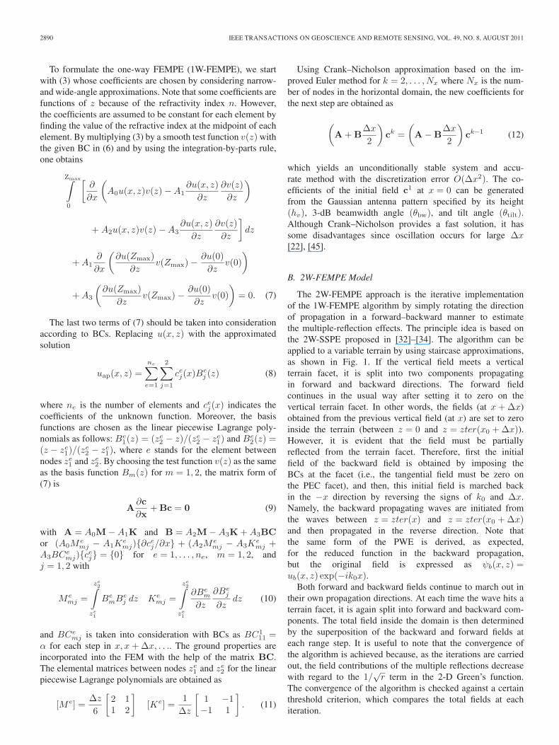
Fig. 13. PF versus height at two specified ranges with the same parameters asin Fig. 12. SSPE (Δz = 0.33 m and Δx = 100 m). FEMPE (Δz = 0.33 mand Δx = 12.5 m).

accuracy limit). The propagation factor (PF) versus height at35- and 50-km ranges of this scenario is shown in Fig. 13.At 35-km range, forward propagating waves interfere with thebackward reflected waves (from the knife-edge wall) and edge-diffracted waves (from the top of the knife-edge wall). Sincethe forward-propagated and backward-reflected contributionsare stronger than the edge-diffracted contributions, excellentagreement among the three models is obtained. It is observedthat multiple reflections (almost resonance behavior) occur inthe region between the walls. It is known that the GTD is ahigh-frequency asymptotic method; whereas, the FEMPE andSSPE approaches can account for the diffraction effects upto a certain extent. In comparing the 2W-FEMPE with theGO+UTD approach, the contribution of the waves hitting thewalls up to three times is superposed. To have fair comparisonsup to third degree of reflections, the GO+UTD code is devel-oped to account for 35 types of rays bouncing from the wallsand the ground, in accordance with the LOS criteria. Theserays include the reflected waves up to third degree, as wellas the diffracted waves from the finite-height wall. Excellentagreement among the results verifies the performance of the2W-FEMPE with respect to the GO+UTD approach. However,the multiple bouncing of the diffracted fields from the walls andthe ground is ignored in the GO+UTD code due their negligibleeffects compared with strong reflections. Therefore, a littlediscrepancy among the results appears there, as expected.

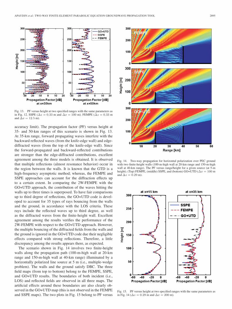
The scenario shown in Fig. 14 involves two finite-heightwalls along the propagation path (100-m-high wall at 20-kmrange and 150-m-high wall at 40-km range) illuminated by ahorizontally polarized line source at 5 m (i.e., multiple-wedgeproblem). The walls and the ground satisfy DBC. The threefield maps (from top to bottom) belong to the FEMPE, SSPE,and GO+UTD results. The boundaries of both incident (i.e.,LOS) and reflected fields are observed in all three maps. Theartificial effects around these boundaries are also clearly ob-served in the GO+UTD map (this is not observed in the FEMPEand SSPE maps). The two plots in Fig. 15 belong to PF versus

Fig. 14. Two-way propagation for horizontal polarization over PEC groundwith two finite-height walls (100-m-high wall at 20-km range and 150-m-highwall at 40-km range). The PF versus range/height for a given source (at 5-mheight). (Top) FEMPE, (middle) SSPE, and (bottom) GO+UTD (Δx = 100 mand Δz = 0.29 m).

Fig. 15. PF versus height at two specified ranges with the same parameters asin Fig. 14 (Δz = 0.29 m and Δx = 200 m).

2896 IEEE TRANSACTIONS ON GEOSCIENCE AND REMOTE SENSING, VOL. 49, NO. 8, AUGUST 2011

Fig. 16. Two-way propagation for vertical polarization over PEC ground withtwo infinite-height walls at 0 and 60 km. The PF versus range/height for agiven source (at 30-km range and 100-m height). (Top) Image method and(bottom) FEMPE method, where f = 3 GHz, Δz = 0.33 m, Δx = 25 m.# of images = 5, and # of reflection = 1.

height at two different ranges, showing the comparison amongthe three models. At the bottom left, the range is 15 km, whichis in the interference region. The range at the bottom right is35 km, which is in the shadow/diffraction region. As observed,excellent agreement is obtained in the first region again, buta discrepancy is observed in the shadow region. Note that therealization of the line-source excitation in the FEMPE at leastin its current piecewise linear model is almost impossible (itis known that source modeling requires additional effort inany variant of FEM approach); therefore, the SSPE-propagatedvertical field profile, which is a few wavelengths away from thesource, can be used as the initial source profile of the FEMPEmodel.

To confirm these speculations, the propagation scenario forvertical polarization between two infinite-extent walls withinfinite number of reflections from both ends (i.e., with infinitenumber of images) is taken into account. The image method isused as follows. There is a single ground image of the source.First, the ground is removed and an image is placed to representthe ground. The source is vertically polarized; therefore, NBCis required at the bottom. However, there is an infinite numberof images because of the two walls. The source in this case isparallel to both walls, which means that DBC must be taken intoaccount on the walls. The 3-D field map versus range/heightof this scenario is shown in Fig. 16. The PF versus height at40- and 50-km ranges, computed with GO+GTD, FEMPE, andSSPE models, is shown in Fig. 17. Excellent agreement amongthe models show that the 2W-FEMPE (also, the 2W-SSPE) canaccount for even highly resonating interferences. Note that thediscrepancy at short ranges in the vicinity of the line sourceis just because of the inefficiency in the FEMPE model inrepresenting the line source.

Finally, Figs. 18 and 19 belong to arbitrary terrain profileswhich do not have any analytical exact or approximate solution

Fig. 17. PF versus height at two specified ranges with the same parametersas in Fig. 16. SSPE (Δz = 0.16 m and Δx = 100 m) and FEMPE (Δz =0.33 m and Δx = 12.5 m).

Fig. 18. Two-way propagation over arbitrary terrain through homogeneousstandard atmosphere. The PF versus range/height for a given source (hv1 =150 m, θbw1 = 1◦, θtilt1 = −25◦, hv2 = 200 m, θbw2 = 1◦, and θtilt2 =−5◦). (Top) Narrow FEMPE and (bottom) wide FEMPE, with f = 600 MHz,Δz = 0.42 m, and Δx = 1 m in 50 min.

that might serve as reference and where only the FEMPEmodel can be compared with the SSPE model for horizontalpolarization. Fig. 18 shows the comparison of narrow- andwide-angle FEMPE results. As observed, narrow-angle FEMPEcannot accurately account for the reflections which changethe true field map considerably. The 3-D field maps versusrange/height of another scenario produced with the 2W-FEMPEand 2W-SSPE models are shown in Fig. 19.

Note that Figs. 18 and 19 need further comparisons againstother full wave (e.g., the Method of Moments (MoM)-based[48]–[50] and/or the time-domain propagation [51]–[54]) mod-els in order to complete the VV&C tests. This is becauseboth SSPE and FEMPE approaches start with the same PEmodel and equally inherit all modeling incapabilities (e.g., the

APAYDIN et al.: TWO-WAY FINITE-ELEMENT PARABOLIC EQUATION GROUNDWAVE PROPAGATION TOOL 2897

Fig. 19. Two-way propagation over arbitrary terrain through inhomogeneousatmosphere. The PF versus range/height for a given source (hv = 400 m,θbw = 0.5◦, θtilt = −0.5◦). (Top) FEMPE and (bottom) SSPE, with f =300 MHz, Δz = 1 m, and Δx = 200 m, with refractivity slope of −200Munit/km between 300 and 400 m (ducting case). tfempe = 7 min andtsspe = 30 s.

Fig. 20. Two-way propagation over arbitrary terrain through inhomogeneousatmosphere. The PF versus range at z = 250 m for the given source (hv =400 m, θbw = 0.5◦, and θtilt = −0.5◦) using 2W-SSPE and 2W-FEMPE(f = 300 MHz, Δz = 1 m, and Δx = 200 m, with refractivity slope of−200 Munit/km between 300 and 400 m (ducting case), tfempe = 7 min, andtsspe = 30 s).

paraxial approximation). Yet, analytical exact solutions havenot appeared for the irregular terrain models. The asymptoticGO+UTD model is not applicable (in its current form) toproblems containing irregular terrains (which is beyond thescope of this study). To support this speculation, the PF versusrange extracted from the 3-D field maps shown in Fig. 19is plotted in Fig. 20. Here, the horizontal PF is plotted from20 to 60 km, which is the range of interference of forward-and backward-propagated waves. As observed, there is a goodagreement between the results of the 2W-FEMPE and 2W-SSPE models, but this is not as good as the agreement obtainedin other examples.

V. CONCLUSION

A 2W-FEMPE algorithm has been developed, tested, andcalibrated against scenarios with analytical exact solutions,such as the modal summation, image method, and asymptoticmodels, such as GO+UTD models. Tests and comparisonsare also performed against the 2W-SSPE algorithm. Bothnarrow- and wide-angle PE models are used during these testsand comparisons. Excellent agreement obtained from thesetests/comparisons among all the models used show that both ofthe 2W-FEMPE and 2W-SSPE models can be used effectivelyin complex propagation scenarios above the Earth’s surfacethrough inhomogeneous atmosphere.

The FEMPE model needs much smaller range steps thanthe SSPE model and therefore necessitates longer computationtimes when long-range propagation is of interest. According tothe last example (shown in Fig. 19), the computation time ofthe FEMPE is at least 14 times longer as compared with that ofSSPE. As a result, the number of nodes used in the transverseand range coordinates should be optimized with respect to thefollowing parameters: the operating frequency, the irregularterrain structure, inhomogeneous atmosphere, and the selectionof the initial antenna pattern specified by its height, beamwidth,and tilt. Moreover, the line-source excitation is a serious prob-lem in the FEMPE model, but this might be overcome byconstructing the initial field profile at a few wavelengths awayfrom the line source by using some other models such as theSSPE or GO, etc., or using smooth, such as Gaussian-type,source patterns. On the other hand, FEMPE model handles allkinds of BC at the surface much more easily when comparedwith the SSPE model.

REFERENCES

[1] S. Grosdidier, A. Baussard, and A. Khenchaf, “HFSW radar model: Sim-ulation and measurement,” IEEE Trans. Geosci. Remote Sens., vol. 48,no. 9, pp. 3539–3549, Sep. 2010.

[2] M. A. Leontovich and V. A. Fock, “Solution of propagation of electro-magnetic waves along the Earth’s surface by the method of parabolicequation,” J. Phys. USSR, vol. 10, pp. 13–23, 1946.

[3] R. H. Hardin and F. D. Tappert, “Applications of the split-step Fouriermethod to the numerical solution of nonlinear and variable coefficientwave equations,” SIAM Rev., vol. 15, p. 423, 1973.

[4] J. R. Kuttler and G. D. Dockery, “Theoretical description of the parabolicapproximation/Fourier split-step method of representing electromagneticpropagation in the troposphere,” Radio Sci., vol. 26, no. 2, pp. 381–393,1991.

[5] A. E. Barrios, “Parabolic equation modeling in horizontally inhomoge-neous environments,” IEEE Trans. Antennas Propag., vol. 40, no. 7,pp. 791–797, Jul. 1992.

[6] A. E. Barrios, “A terrain parabolic equation model for propagation in thetroposphere,” IEEE Trans. Antennas Propag., vol. 42, no. 1, pp. 90–98,Jan. 1994.

[7] R. Janaswamy, “A curvilinear coordinate-based split-step parabolic equa-tion method for propagation predictions over terrain,” IEEE Trans. Anten-nas Propag., vol. 46, no. 7, pp. 1089–1097, Jul. 1998.

[8] C. A. Zelley and C. C. Constantinou, “A three-dimensional parabolicequation applied to VHF/UHF propagation over irregular terrain,” IEEETrans. Antennas Propag., vol. 47, no. 10, pp. 1586–1596, Oct. 1999.

[9] M. F. Levy, Parabolic Equation Methods for Electromagnetic Wave Prop-agation. London, U.K.: IEE, 2000.

[10] C. Mias, “Fast computation of the nonlocal boundary condition in finitedifference parabolic equation radiowave propagation simulations,” IEEETrans. Antennas Propag., vol. 56, no. 6, pp. 1699–1705, Jun. 2008.

[11] P. D. Holm, “Wide-angle shift-map PE for a piecewise linear terrain—A finite-difference approach,” IEEE Trans. Antennas Propag., vol. 55,no. 10, pp. 2773–2789, Oct. 2007.

2898 IEEE TRANSACTIONS ON GEOSCIENCE AND REMOTE SENSING, VOL. 49, NO. 8, AUGUST 2011

[12] D. J. Donohue and J. R. Kuttler, “Propagation modeling over terrain usingthe parabolic wave equation,” IEEE Trans. Antennas Propag., vol. 48,no. 2, pp. 260–277, Feb. 2000.

[13] L. Sevgi, F. Akleman, and L. B. Felsen, “Groundwave propagationmodeling: Problem-matched analytical formulations and direct numericaltechniques,” IEEE Antennas Propag. Mag., vol. 44, no. 1, pp. 55–75,Feb. 2002.

[14] L. Sevgi, Complex Electromagnetic Problems and Numerical SimulationApproaches. Piscataway, NJ: IEEE Press, Jun. 2003.

[15] L. Sevgi, C. Uluisik, and F. Akleman, “A Matlab-based two-dimensionalparabolic equation radiowave propagation package,” IEEE AntennasPropag. Mag., vol. 47, no. 4, pp. 164–175, Aug. 2005.

[16] L. Sevgi, “Groundwave modeling and simulation strategies and path lossprediction virtual tools,” IEEE Trans. Antennas Propag., vol. 55, no. 6,pp. 1591–1598, Jun. 2007, (Special issue on Electromagnetic Wave Prop-agation in Complex Environments: A Tribute to L. B. Felsen).

[17] D. A. Hill and J. R. Wait, “HF ground wave propagation over mixed land,sea, and sea-ice paths,” IEEE Trans. Geosci. Remote Sens., vol. GRS-19,no. 4, pp. 210–216, Oct. 1981.

[18] D. Huang, “Finite element solution to the parabolic wave equation,”J. Acoust. Soc. Am., vol. 84, no. 4, pp. 1405–1413, Oct. 1988.

[19] K. Arshad, F. A. Katsriku, and A. Lasebae, “An investigation of tropo-spheric radio wave propagation using finite elements,” WSEAS Trans.Communications, vol. 4, no. 11, pp. 1186–1192, Nov. 2005.

[20] G. Apaydin and L. Sevgi, “FEM-based surface wave multi-mixed-pathpropagator and path loss predictions,” IEEE Antennas Wireless Propag.Lett., vol. 8, pp. 1010–1013, 2009.

[21] G. Apaydin and L. Sevgi, “Numerical investigations of and path loss pre-dictions for surface wave propagation over sea paths including hilly islandtransitions,” IEEE Trans. Antennas Propag., vol. 58, no. 4, pp. 1302–1314, Apr. 2010.

[22] G. Apaydin and L. Sevgi, “The split step Fourier and finite elementbased parabolic equation propagation prediction tools: Canonical tests,systematic comparisons, and calibration,” IEEE Antennas Propag. Mag.,vol. 52, no. 3, pp. 66–79, Jun. 2010.

[23] D. J. Thomson and N. R. Chapman, “A wide-angle split-step algorithmfor the parabolic equation,” J. Acoust. Soc. Am., vol. 74, no. 6, pp. 1848–1854, Dec. 1983.

[24] M. D. Collins, “A split-step Pade solution for the parabolic wave equa-tion,” J. Acoust. Soc. Am., vol. 93, no. 4, pp. 1736–1742, Apr. 1993.

[25] J. R. Kuttler, “Differences between the narrow-angle and wide-anglepropagators in the split-step Fourier solution of the parabolic wave equa-tion,” IEEE Trans. Antennas Propag., vol. 47, no. 7, pp. 1131–1140,Jul. 1999.

[26] M. F. Levy, “Diffraction studies in urban environment with wide-angleparabolic equation method,” Electron. Lett., vol. 28, no. 16, pp. 1491–1492, Jul. 1992.

[27] L. A. Weinstein, Open Resonators and Open Waveguides. Boulder, CO:Golem Press, 1969.

[28] P. Y. Ufimtsev, “Current waves in a thin wire and in a ribbon,” U.S.S.R.,Comput. Math. Math. Phys., vol. 8, no. 6, pp. 250–261, 1968.

[29] P. Y. Ufimtsev, Theory of Edge Diffraction in Electromagnetics. Encino,CA: Tech Science Press, 2003.

[30] P. Y. Ufimtsev, Theory of Edge Diffraction in Electromagnetics: Origina-tion and Validation of the Physical Theory of Diffraction. Raleigh, NC:SciTech Publishing, Inc., 2009.

[31] P. Y. Ufimtsev and S. A. P. Krasnozhen, “Current waves in a straight thinwire resonators with finite conductivity,” Electromagnetics, vol. 12, no. 2,pp. 121–132, 1992.

[32] M. D. Collins, “A two-way parabolic equation for elastic media,”J. Acoust. Soc. Amer., vol. 93, no. 4, pp. 1815–1825, Apr. 1993.

[33] J. F. Lingevitch, M. D. Collins, M. J. Mills, and R. B. Evans, “A two-wayparabolic equation that accounts for multiple scattering,” J. Acoust. Soc.Am., vol. 112, no. 2, pp. 476–480, Aug. 2002.

[34] M. J. Mills, M. D. Collins, and J. F. Lingevitch, “Two-way parabolic equa-tion techniques for diffraction and scattering problems,” Wave Motion,vol. 31, no. 2, pp. 173–180, Feb. 2000.

[35] H. Orazi and S. Hosseinzadeh, “Radio-wave-propagation modeling in thepresence of multiple knife edges by the bidirectional parabolic-equationmethod,” IEEE Trans. Veh. Technol., vol. 56, no. 3, pp. 1033–1040,May 2007.

[36] O. Ozgun, “Recursive two-way parabolic equation approach for model-ing terrain effects in tropospheric propagation,” IEEE Trans. AntennasPropag., vol. 57, no. 9, pp. 2706–2714, Sept. 2009.

[37] G. Apaydin, O. Ozgun, M. Kuzuoglu, and L. Sevgi, “Two-way split-step Fourier and finite element based parabolic equation propagationtools: Comparisons and calibration,” in Proc. IEEE Int. Symp. Antennas

Propagation USNC/URSI Nat. Radio Sci. Meet., Toronto, ON, Canada,July 11–17, 2010, pp. 1–4.

[38] O. Ozgun, G. Apaydin, M. Kuzuoglu, and L. Sevgi, “Two-way Fouriersplit step algorithm over variable terrain with narrow and wide angle prop-agators,” in Proc. IEEE Int. Symp. Antennas Propagation USNC/URSINat. Radio Sci. Meet., Toronto, ON, Canada, July 11–17, 2010, pp. 1–4.

[39] J. B. Keller, “Geometrical theory of diffraction,” J. Opt. Soc. Amer.,vol. 52, no. 2, pp. 116–130, 1962.

[40] R. G. Kouyoumjian and P. H. Pathak, “A uniform geometrical theory ofdiffraction for an edge in a perfectly conducting surface,” Proc. IEEE,vol. 62, no. 11, pp. 1448–1461, Nov. 1974.

[41] P. Y. Ufimtsev, Fundamentals of the Physical Theory of Diffraction.Hoboken, NJ: Wiley, 2007.

[42] L. Sevgi, “Guided waves and transverse fields: Transverse to what?,”IEEE Antennas Propag. Mag., vol. 50, no. 6, pp. 221–225, Dec. 2008.

[43] J. R. Wait, “The scope of impedance boundary conditions in radio prop-agation,” IEEE Trans. Geosci. Remote Sens., vol. 28, no. 4, pp. 721–723,Jul. 1990.

[44] J. Volakis, A. Chatterjee, and L. Kempel, Finite Element Method forElectromagnetics: Antennas, Microwave Circuits, and Scattering Appli-cations. Piscataway, NJ: IEEE Press, 1998.

[45] J.-M. Jin, The Finite Element Method in Electromagnetics. New York:Wiley, 2002.

[46] W. Y. Yang, W. Cao, T. Chung, and J. Morris, Applied Numerical MethodsUsing Matlab. Hoboken, NJ: Wiley, 2005.

[47] G. Apaydin and L. Sevgi, “Validation, verification and calibration in ap-plied computational electromagnetics,” in Proc. 26th Int. Rev. Progr. Appl.Comput. Electromagn., Tampere, Finland, Apr. 25–29, 2010, pp. 679–684.

[48] C. A. Tunc, A. Altintas, and V. B. Erturk, “Examination of existentpropagation models over large inhomogeneous terrain profiles using fastintegral equation solution,” IEEE Trans. Antennas Propag., vol. 53, no. 9,pp. 3080–3083, Sep. 2005.

[49] C. Tunc, F. Akleman, V. Erturk, A. Altintas, and L. Sevgi, “Fast integralequation solutions: Application to mixed path terrain profiles and compar-isons with parabolic equation method,” Complex Comput. Netw., vol. 104,Springer Proc. Phys., pp. 55–63, Jan. 2006.

[50] A. Yagbasan, C. A. Tunc, V. B. Erturk, A. Altintas, and R. Mittra, “Char-acteristic basis function method for solving electromagnetic scatteringproblems over rough terrain profiles,” IEEE Trans. Antennas Propag.,vol. 58, no. 5, pp. 1579–1589, May 2010.

[51] F. Akleman and L. Sevgi, “A novel finite-difference time-domain wavepropagator,” IEEE Trans. Antennas Propag., vol. 48, no. 5, pp. 839–841,May 2000.

[52] F. Akleman and L. Sevgi, “Time and frequency domain wave propa-gators,” ACES J. Special Issue Comput. Electromagn. Techn. WirelessCommun., vol. 15, no. 3, pp. 186–201, Nov. 2000.

[53] M. O. Ozyalcin, F. Akleman, and L. Sevgi, “A novel TLM-based time-domain wave propagator,” IEEE Trans. Antennas Propag., vol. 51, no. 7,pp. 1679–1680, Jul. 2003.

[54] F. Akleman and L. Sevgi, “Realistic surface modeling for a finite-difference time-domain wave propagator,” IEEE Trans. AntennasPropag., vol. 51, no. 7, pp. 1675–1679, Jul. 2003.

Gökhan Apaydin (M’08–SM’11) received the B.S.,M.S., and Ph.D. degrees in electrical and electron-ics engineering from Bogazici University, Istanbul,Turkey, in 2001, 2003, and 2007, respectively.

From 2001 to 2005, he was a Teaching andResearch Assistant with Bogazici University. From2005 to 2010, he was a Project and ResearchEngineer with the Applied Research and Devel-opment, University of Technology Zurich, Zurich,Switzerland. Since 2010, he has been with ZirveUniversity, Gaziantep, Turkey. He has been working

on several research projects on electromagnetic (EM) propagation, the develop-ment of a finite-element method for EM computation, positioning, filter design,and related areas. He has (co)authored 14 journals and 27 conference papersand technical reports at the Hochschule für Technik Zürich, Zürich.

APAYDIN et al.: TWO-WAY FINITE-ELEMENT PARABOLIC EQUATION GROUNDWAVE PROPAGATION TOOL 2899

Ozlem Ozgun (M’05) received the B.Sc. and M.Sc.degrees in electrical engineering from Bilkent Uni-versity, Ankara, Turkey, in 1998 and 2001, respec-tively, and the Ph.D. degree in electrical engineeringfrom the Middle East Technical University (METU),Ankara, in 2007.

She is currently an Assistant Professor withMETU—Northern Cyprus Campus, Mersin, Turkey.From 2007 to 2008, she was with the Electro-magnetic Communication Laboratory, PennsylvaniaState University, University Park; ASELSAN Inc.,

Ankara, from 2004 to 2005; TUBITAK-UEKAE, National Research Institute ofElectronics and Cryptology, Ankara, from 2000 to 2004; and Bilkent Universityfrom 1998 to 2000. Her main research interests include computational elec-tromagnetics, finite-element method, domain decomposition, electromagnetic(EM) propagation and scattering, metamaterials, and stochastic EM problems.

Mustafa Kuzuoglu (M’92) received the B.Sc.,M.Sc., and Ph.D. degrees in electrical engineer-ing from the Middle East Technical University(METU), Ankara, Turkey, in 1979, 1981, and 1986,respectively.

He is currently a Professor with METU. His re-search interests include computational electromag-netics, inverse problems, and radars.

Levent Sevgi (M’99–SM’02–F’09) received thePh.D. degree from Istanbul Technical University,Istanbul, Turkey, and Polytechnic Institute of NewYork University, Brooklyn, in 1990. Prof. Leo Felsenwas his advisor.

He was with Istanbul Technical University from1991 to 1998; TUBITAK-MRC, Information Tech-nologies Research Institute, Gebze/Kocaeli, Turkey,from 1999 to 2000; Weber Research Institute/Polytechnic University of New York, from 1988 to1990; Scientific Research Group of Raytheon Sys-

tems, Canada, from 1998 to 1999; and the Center for Defense Studies, ITUV-SAM, from 1993 to 1998 and from 2000 to 2002. Since 2001, he has been withDogus University, Istanbul. He has been involved with complex electromag-netic (EM) problems and systems for more than 20 years. His research studyhas focused on propagation in complex environments, analytical and numericalmethods in electromagnetics, EMC/EMI modeling and measurement, radarand integrated surveillance systems, surface-wave HF radars, finite-differencetime domain, TLM, finite-element method, split-step parabolic equation, andMethod of Moments techniques and their applications, radar cross-sectionmodeling, and bioelectromagnetics. He is also interested in novel approaches inengineering education and teaching electromagnetics via virtual tools. He alsoteaches popular science lectures such as science, technology, and society.

Prof. Sevgi is the Writer/Editor of the “Testing ourselves” Column in theIEEE Antennas and Propagation Magazine, a member of the IEEE Antennasand Propagation Society Education Committee, and the “Scientific Literacy”Column Writer of the IEEE Region 8 Newsletter.