A novel algorithm for distance transformation on irregular isothetic grids

A Novel Algorithm for Distance Transformation

on Irregular Isothetic Grids

Antoine Vacavant1,2, David Coeurjolly1,3, and Laure Tougne1,2

1 Universite de Lyon, CNRS2 Universite Lyon 2, LIRIS, UMR5205, F-69676, France3 Universite Lyon 1, LIRIS, UMR5205, F-69622, France

{antoine.vacavant,david.coeurjolly,laure.tougne}@liris.cnrs.fr

Abstract. In this article, we propose a new definition of the E2DT(Squared Euclidean Distance Transformation) on irregular isothetic gridssuch as quadtree/octree or run-length encoded d-dimensional images.We describe a new separable algorithm to compute this transformationon every grids, which is independent of the background representation.We show that our proposal is able to efficiently handle various kind ofclassical irregular two-dimensional grids in imagery, and that it can beeasily extended to higher dimensions.

1 Introduction

The representation and the manipulation of large-scale data sets by irregulargrids is a today scientific challenge for many applications [9, 12]. Here, we areinterested in discrete distance definition and distance transformation [8, 13] onthis kind of multi-grids to develop fast and adaptive shape analysis tools. TheDistance Transformation (DT) of a binary image consists in labeling each point ofa discrete object E (i.e. foreground) with its shortest distance to the complementof E (i.e. background). This process is widely studied and developed on regulargrids (see for example [4]). Some specific extensions of the DT to non-regulargrids also exist, such as rectangular grids [15], quadtrees [18], etc. This articledeals with generalizing the DT computation on irregular isothetic grids (or I-grid for short) in two dimensions (2-D). The proposed method is easily extensibleto higher dimensions. In 2-D, this kind of grids is defined by rectangular cellswhose edges are aligned along the two axis. The size and position of those non-overlapping cells are defined without constraint (see next section for a formaldefinition). The quadtree decomposition and the RLE (Run Length Encoding)grouping schemes are examples of classical techniques in imagery which inducean I-grid. Here, we focus our interest on generalizing techniques that computethe E2DT (squared Euclidean DT) of a d-dimensional (d-D) binary image [2,10, 14]. Many of those methodologies can be linked to the computation of adiscrete Voronoi diagram of the background pixels [6, 2]. In a previous work [16],we introduced a definition of E2DT on I-grids based on the background cellscenters. After showing the link between this process and the computation of

2 Antoine Vacavant et al.

the Voronoi diagram of those background points, we proposed two completingalgorithms to handle various configurations of I-grids. Unfortunately, we noticedthat they suffer from non-optimal time complexity. Moreover, the result of thistransformation strongly depends on the representation of the background.

In this article, we aim to provide a faster version of our previous separablealgorithm for distance transformation on I-grids such as quadtree or run-codedd-D images. Instead of a center based DT algorithm we now focus on a fasterborder based DT algorithm, by resampling the irregular border part of objectswith a partly regular grid. This paper is organized as follows: (1) we present anew way to compute the E2DT on I-grids, based on the border of the backgroundcells (Section 2). We also illustrate its relation with the computation of a Voronoidiagram of segments; (2) in Section 3, we describe an algorithm based on thework of R. Maurer et al. [10] to efficiently compute this new transformationin 2-D, but extensible to higher dimensions; (3) we finally show in Section 4experimental results to compare our new contribution with the techniques wedeveloped in [16] in terms of speed and time complexity.

2 Distance Transformations on I-grids and Voronoi

Diagrams

In this section, we first recall the concept of irregular isothetic grids (I-grids),with the following definition [1]:

Definition 1 (2-D I-grid). Let I ⊂ R2 be a closed rectangular support. A 2-D

I-grid I is a tiling of I with non overlapping rectangular cells which edges are

parallel to the X and Y axis. The position (xR, yR) and the size (lxR, lyR) of a cell

R in I are given without constraint: (xR, yR) ∈ R2, (lxR, l

yR) ∈ R

2.

We consider this definition of 2-D I-grids for the rest of the paper, and we willshortly show that our contribution is easily extensible to the d-D case. In ourframework, we consider labeled I-grids, i.e. each cell of the grid has a foreground

or background label (its value is respectively ”0” or ”1” for example). For anI-grid I, we denote by IF and IB the sets of foreground and background cells.

We can first consider that the distance between two cells R and R′ is thedistance between their centers. If we denote p = (xR, yR) and p′ = (xR′ , yR′)these points, and d2

e(p, p′) the squared Euclidean distance between them, theI-CDT (Center-based DT on I-grids) of a cell R is defined as follows [16]:

I−CDT(R) = minR′

{

d2

e(p, p′); R′ ∈ IB

}

, (1)

and resumes to the E2DT if we consider I as a regular (square or rectangular)discrete grid. However, this distance is strongly dependent of the backgroundrepresentation. In Figure 1, we present an example of the computation of theI-CDT of two I-grids where only the background cells differ. Since this definitionis based on the cells centers position, the I-CDT do not lead to the same distancemap depending on the background coding.

Distance Transformation on Irregular Grids 3

(a) (b) (c)

Fig. 1. The result of the I-CDT of the complete regular grid (b) computed from thebinary image (a) and an I-grid where the foreground is regular and the background isencoded with a RLE scheme along Y (c). The distance value d of a cell is representedwith a grey level c = d mod 255. The contour of the object (background/foregroundfrontier) is recalled in each distance map (b) and (c) with a smooth curve

We now introduce an alternative definition of the E2DT by consider-ing the shortest distance between a foreground cell center and the back-ground/foreground boundary of the I-grid. We suppose here that the intersectionbetween two adjacent cells is a segment of dimension one (i.e. they respect thee-adjacency relation [1]). Let S be the set of segments at the interface betweentwo adjacent cells R ∈ IF and R′ ∈ IB .The I-BDT (Border-based DT on I-grids)is then defined as follows:

I−BDT(R) = mins

{

d2

e(p, s); s ∈ S}

. (2)

Contrary to the I-CDT given in Equation 1, the result of this process does notdepend on the representation of the background. We can draw a parallel be-tween those extensions of the E2DT to I-grids and the computation of a Voronoidiagram (VD). More precisely, as in the regular case, the I-CDT can be linkedwith the VD of the background cells centers (i.e. Voronoi sites or VD sites) [16].The VD of a set of points P = {pi} is a tiling of the plane into Voronoi cells (orVD cells) {Cpi

} [3]. If we now consider the background/foreground frontier tocompute the I-BDT, our definition implies that we compute a VD of segments,and not a classical VD of points (see Figure 2 for an example of these diagramscomputed on a simple I-grid). Hence, a simple approach to compute the I-CDT is to pre-compute the complete VD of the background points [16], and tolocate foreground points in the VD. In this case, the I-CDT computation hasa O(n log nB) time complexity, where n is the total number of cells, and nB isthe number of background cells. This technique is obviously not computationallyefficient for every grids, and not adapted to dense grids [16]. To compute theI-BDT, a similar synopsis can be drawn, where the computation of the VD ofsegments can be handled in O(nS log2 nS), where nS = 4nB is the total numberof segments belonging to the background/foreground frontier [7]. The extensionof those transformation to d-D I-grids is a hard work. A VD can be computed

in d-D with a O(nB log nB + n⌈d/2⌉B ) time complexity (thanks to a gift-wrapping

approach [3] for example). However, localizing a point in the VD is an arduous


(a) (b)

Fig. 2. Example of the VD of the background points to obtain the I-CDT of a simpleI-grid (a). Background cell centers are depicted in black, and foreground ones in white.Distance values are presented above the cells centers. From the same grid, the compu-tation of the I-BDT (b) implies that we consider the VD of the segments belonging tothe background/foreground frontier

task, and an additional structure like subdivision grids [11] should be constructedto handle this operation.

Hence, we have shown that building the entire VD to obtain the I-BDT isneither computationally efficient for every I-grids, nor easily extensible to higherdimensions. We now propose a separable algorithm to compute the I-BDT thatcan be extented to the d-D case.

3 A New Separable Algorithm to Compute the I-BDT

3.1 R. Maurer et al. E2DT Algorithm on Regular Grids

The main idea of this separable (one phase by dimension) method [4, 10] is thatthe intersection between the complete VD of background pixels (i.e. sites) anda line of the grid can be easily computed, then simplified. Indeed, for a row j,the VD sites can be ”deleted” by respecting three remarks mainly based on themonotonicity of de distance [10]: (1) if we consider the line l : y = j, j ∈ Z, then

(a) (b) (c)

Fig. 3. In a regular grid, when we treat a row l with R. Maurer et al. algorithm, weconsider the VD of background nodes like in (a). We only keep the nearest VD sitesof l (b). We obtain (c) by deleting sites which associated VD cells intersect the l row.Arrows indicate the associated VD site of each foreground pixel of this row

we only have to keep the nearest VD sites from l (Figure 3-b), (2) those sites


can be ordered along the X axis, which means that it is not necessary to keepthe complete VD, but only its intersection with the line l, (3) a VD site may behidden by two neighbour sites, and thus not considered anymore (Figure 3-c).In this article, we show the extension of this technique on I-grids by adaptingthese properties on these grids.

3.2 Separable Computation of the I-BDT

To develop a separable process on I-grids, we use a similar structure as theirregular matrix A associated to a labeled I-grid I introduced in [16]. This datastructure aims to organize the cells of the grid along the X and Y axis byadding virtual cells centers (see Figure 4 for an example). We used it in ourprevious work to adapt the separable E2DT algorithm of T. Saito et al. [14],devoted to compute the I-CDT on I-grids. The irregular matrix contains as

(a) (b)

Fig. 4. Construction of the irregular matrix associated to the simple I-grid illustratedin Figure 2. In (a), the extra node A(0, 2) of the matrix is depicted at the intersectionof the dotted lines. New nodes have the same value as the cell containing them. Forthe I-BDT, we also need the shortest distance between a node in respect to its neigh-bour nodes and the border of the cell containing it (b). Examples of values for borderattributes are also given along X (dashed lines) and Y (dotted lines). For instance, wehave HT (1, 1) = HB(1, 1) = 0 since this node coincides with a cell horizontal border.We can also notice that HL(2, 3) 6= HR(2, 3)

many columns (respectively rows) as X-coordinates (Y -coordinates) in the grid.These coordinates are stored in two tables TX and TY (and we denote n1 = |TX |and n2 = |TY |). At the intersection of two X and Y coordinates, a node in Ahas the same value as the cell containing it, and may represent the cell centeror not (i.e. this is an extra node, see Figure 4-a). The extra nodes are used topropagate the distance values through the irregular matrix and then computea correct distance value for each cell center. To apply the I-BDT on this datastructure, we also have to take into account the border and the size of the treatedcells. We thus add for each node A(i, j) border attributes along X and Y axisthat permit to propagate the distance values to cell borders through A. For anode A(i, j) contained by the cell R in I, we denote respectively by HL(i, j) andHR(i, j) the attributes that represent the minimum between the distance to theleft (respectively right) border of R along X , and the distance to the neighbour


node at the left (right) position in A. In the same manner, we define HT (i, j)and HB(i, j) in respect to the top (bottom) border of R and neighbour nodes atthe top (bottom) position in A (see Figure 4-b). Building the irregular matrixof an I-grid I can be handled in O(n1n2) time complexity. More precisely, wefirst scan all the cells of I to know the n1 columns and the n2 rows of A. Then,we consider each node of A and we assign its background or foreground valueand its border attributes.

Equation 2 can now be adapted on the irregular matrix with a minimizationprocess along the two axis (see [17] for the proof):

Proposition 1 (Separable I-BDT). Let A be the associated irregular matrix

of the 2-D I-grid I. Then the I-BDT of I can be decomposed in two separable

processes, and consists in computing the matrix B and C as follows:

B(i, j) = minx

{

min(

|TX(i) − TX(x) − HR(x, j)|, |TX(x) − TX(i) − HL(x, j)|)

;

x ∈ {0, ..., n1 − 1}, A(x, j) = 0}

,

C(i, j) = miny

{

Gy(j); y ∈ {0, . . . , n2 − 1}}

,

where Gy(j) is a flattened parabola given by:

Gy(j) =

B(i, y)2 + (TY (j) − TY (y) − HT (i, y))2 if TY (j) − TY (y) > HT (i, y)B(i, y)2 + (TY (y) − TY (j) − HB(i, y))2 if TY (y) − TY (j) > HB(i, y)B(i, y)2 otherwise.

Fig. 5. Important features of a flattened parabola, composition of two half-parabolas(in dotted lines) and a constant function

We proove in [17] that this proposition is correct, i.e. this two-dimensionalscheme consists in computing the I-BDT given in Equation 2. This separableminimization process also permits to compute the I-CDT (Equation 1), if weassign all border attributes to zero. In this case, this transformation is equiv-alent to a minimization process of a 2-D quadratic form [16], and we considera set of classical parabolas along the Y axis, as in the regular case [14]. Here,


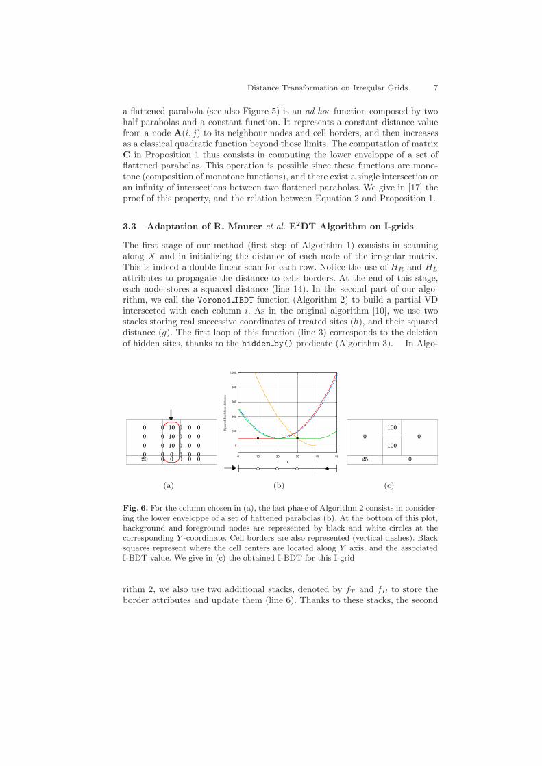
a flattened parabola (see also Figure 5) is an ad-hoc function composed by twohalf-parabolas and a constant function. It represents a constant distance valuefrom a node A(i, j) to its neighbour nodes and cell borders, and then increasesas a classical quadratic function beyond those limits. The computation of matrixC in Proposition 1 thus consists in computing the lower enveloppe of a set offlattened parabolas. This operation is possible since these functions are mono-tone (composition of monotone functions), and there exist a single intersection oran infinity of intersections between two flattened parabolas. We give in [17] theproof of this property, and the relation between Equation 2 and Proposition 1.

3.3 Adaptation of R. Maurer et al. E2DT Algorithm on I-grids

The first stage of our method (first step of Algorithm 1) consists in scanningalong X and in initializing the distance of each node of the irregular matrix.This is indeed a double linear scan for each row. Notice the use of HR and HL

attributes to propagate the distance to cells borders. At the end of this stage,each node stores a squared distance (line 14). In the second part of our algo-rithm, we call the Voronoi IBDT function (Algorithm 2) to build a partial VDintersected with each column i. As in the original algorithm [10], we use twostacks storing real successive coordinates of treated sites (h), and their squareddistance (g). The first loop of this function (line 3) corresponds to the deletionof hidden sites, thanks to the hidden by() predicate (Algorithm 3). In Algo-

(a) (b) (c)

Fig. 6. For the column chosen in (a), the last phase of Algorithm 2 consists in consider-ing the lower enveloppe of a set of flattened parabolas (b). At the bottom of this plot,background and foreground nodes are represented by black and white circles at thecorresponding Y -coordinate. Cell borders are also represented (vertical dashes). Blacksquares represent where the cell centers are located along Y axis, and the associatedI-BDT value. We give in (c) the obtained I-BDT for this I-grid

rithm 2, we also use two additional stacks, denoted by fT and fB to store theborder attributes and update them (line 6). Thanks to these stacks, the second


Algorithm 1: Separable computation of the I-BDT inspired from [10].

input : the labeled I-grid I.output: the I-BDT of I, stored in the irregular matrix C.build the irregular matrix A associated to I;1

for j = 0 to n2 − 1 do {First stage along X}2

if A(0, j) = 0 then B(0, j)← 0;3

else B(0, j)←∞;4

for i = 1 to n1 − 1 do5

if A(i, j) = 0 then B(i, j)← 0;6

else7

if B(i− 1, j) = 0 then B(i, j)← TX(i)− TX(i− 1)−HR(i− 1, j);8

else B(i, j)← TX(i)− TX(i− 1) + B(i− 1, j);9

for i = n1 − 2 to 0 do10

if B(i + 1, j) < B(i, j) then11

if B(i + 1, j) = 0 then B(i, j)← TX(i + 1)− TX(i)−HL(i, j);12

else B(i, j)← TX(i + 1)− TX(i) + B(i− 1, j);13

B(i, j)← B(i, j)2;14

for i = 0 to n1 − 1 do {Second stage along Y }15

Voronoi IBDT(i);16

Algorithm 2: Function Voronoi IBDT() to build a partial VD along Y .

input : the column i of the irregular matrix B.output: the I-BDT of each node of the column i stored in the matrix C.l ← 0, g ← ∅, h← ∅, fT ← ∅, fB ← ∅;1

for j = 0 to n2 − 1 do2

if B(i, j) 6=∞ then3

while l ≥ 2 ∧ hidden by`

g[l − 1], g[l],B(i, j), h[l − 1], h[l], TY (j)´

do4

l← l − 1;5

l← l + 1, g[l]← A(i, j), h[l]← TY (j), fT [l]← HT (i, j), fB ← HB(i, j);6

if (ns ← l) = 0 then return;7

l ← 1;8

for j = 0 a n2 − 1 do9

while l < ns ∧ Gl(j) > Gl+1(j) do l← l + 1;10

A(i, j)← Gl(j);11

Algorithm 3: Predicate hidden by().

input : Y -coordinates of three points in R2 denoted by uy , vy, wy , and their

squared distance to the line L : y = r denoted by d2e(u, L), d2

e(v, L),d2

e(w, L).output: is v hidden by u and w ?a← vy − uy , b← wy − vy , c← a + b;1

return c× d2e(v, L)− b× d2

e(u, L)− a× d2e(w, L)− abc > 0;2


stage of our algorithm is achieved in linear time. By testing the value of l (line 7),we know if we have to scan again the stacks and to update the distance values ofthe nodes. Finally, we linearly scan the stacks to find the nearest border of theA(i, j) current node (line 10), and this step indeed consists in considering thelower enveloppe of a set of flattened parabolas {Gl}, given by (see also Figure 6):

Gl(j) =

g[l] + (TY (j) − h[l] − fT [l])2 if TY (j) − h[l] > fT [l]g[l] + (h[l] − TY (j) − fB[l])2 if TY (j) − h[l] > fB[l]B(i, y)2 else,

(3)

which is the adaptation of Proposition 1 with the stacks g, h, fT and fB. Weproove in [17] that this adaptation is correct, i.e. it computes a correct distancemap for I-BDT.

As a consequence, we have described a linear I-BDT algorithm in respect tothe associated irregular matrix size, i.e. in O(n1n2) time complexity. Our newcontribution is easily extensible to higher dimensions: we still realize the firststep as an initialization phase, and for each dimension d > 1, we combine resultsobtained in dimension d-1. If we consider a labeled d-D I-grid, which associatedirregular matrix size is n1 × · · · × nd, the time complexity of our algorithm isthus in O(n1 × · · · × nd). In the next section, we present experiments to showthe interest of the I-BDT, and to point out that our algorithm is a very efficientapproach to compute both I-CDT and I-BDT of various classical I-grids.

4 Experimental Results

We first propose to present the result of our I-BDT algorithm for the binaryimage depicted at the beginning of this article in Figure 1, digitized in variousclassical I-grids used in imagery. Table 1 illustrates I-BDT elevation maps wherethe background and the foreground of the original image are independently rep-resented with a regular square grid (D), a quadtree (qT) and a RLE along Y

(L). We can notice in this figure that the result of the I-BDT is independentof the representation of the background. The distance values in the foregroundregion are thus the same in the three elevation maps of a given column.

We now focus our interest on the execution time of our new algorithm, inrespect to our previous work [16]. We consider the three algorithms presentedin Table 2. The first algorithm represents the simple approach we discussedin Section 2, which is hardly extensible to d-D treatments, and I-BDT compu-tation. Algorithm 2 is described in [16] and is inspired from the quadradic formminimization scheme of T. Saito et al. [14]. Thanks to the flattened paraboladefinition, we can extend this algorithm to I-BDT, but with a non-optimal timecomplexity, in respect to the irregular matrix size. Algorithm 3 is our new sepa-rable transformation inspired from [10]. In Figure 7, we present the three chosenimages for our experiments, and in Table 3, we show the execution times forthese three algorithms, for I-grids built from three binary images. We have per-formed those experiments on a mobile workstation with a 2.2 Ghz Intel CentrinoDuo processor, and 2 Gb RAM. We can first notice that our new contribution


(a) noise (b) lena (c) canon

Fig. 7. For the images noise (100x100), lena (208x220), canon (512x512) we considerin our experiments the associated I-grids (regular grid, quadtree decomposition andRLE along Y scheme)

Table 1. Elevation maps representing the I-BDT of each I-grid. X and Y are the axisof the image, and Z corresponds to the distance value. The foreground (columns) andthe background (rows) of the image are digitized independently. The color palette isdepicted on the right of the figure

Foreground

D qT L

Background D

qT

L

Table 2. The three compared algorithms, and their associated time and space com-plexities. We also check if an algorithm is extensible to d-D I-grids and what kind oftransformation it can perform (I-CDT, I-BDT)

Id. Algorithm Time Space d-D I-CDT I-BDT

1 Complete VD [16] O(n log nB) O(n) X

2 From T. Saito et al. [14, 16] O(n1n2 log n2) O(n1n2) X X X

3 From R. Maurer et al. [10] O(n1n2) O(n1n2) X X X


Table 3. We present execution times (in seconds) for each algorithm for the I-CDT(a) and the I-BDT (b) and for each I-grid. Number inside parenthesis in (b) are theincreasing rate in % between I-CDT and I-BDT execution times

(a) I-CDT

ImageAlgorithm 1

D qT L

noise 0.255 0.104 0.053lena 1.413 0.145 0.081

canon 36.236 0.273 0.234

ImageAlgorithm 2

D qT L

noise 0.037 0.077 0.044lena 0.192 0.376 0.245

canon 1.678 1.322 1.316

ImageAlgorithm 3

D qT L

noise 0.046 0.065 0.038lena 0.185 0.166 0.135

canon 1.134 0.485 0.585

(b) I-BDT

ImageAlgorithm 2

D qT L

noise 0.047 (27) 0.100 (29) 0.054 (23)lena 0.256 (33) 0.491 (31) 0.320 (31)

canon 2.248 (34) 2.107 (59) 2.020 (53)

ImageAlgorithm 3

D qT L

noise 0.065 (42) 0.085 (31) 0.049 (29)lena 0.258 (40) 0.209 (26) 0.170 (26)

canon 1.507 (33) 0.563 (16) 0.718 (23)

gives good results for I-CDT. Indeed, Algorithm 3 is the fastest one for denseI-grids (regular grids or L for noise), and is very competitive for sparse I-grids(e.g. near one half second for qT and L based on image canon). In the latter case(canon), Algorithm 1 is slightly faster than our approach, but we recall that itis hardly extensible to higher dimensions. Algorithm 2, which we developped inour previous work [16], was interesting for dense grids, and is now overtaken byAlgorithm 3. For the I-BDT, Algorithm 2 and 3 suffer from an execution timeincrease, mainly due to the integration of the complex flattened parabola. Butour contribution remains as the fastest algorithm, and the time increasing rateis moderate for the tested grids. Large sparse I-grids like qT and L based oncanon are still handled in less than one second.

5 Conclusion and Future Works

In this article, we have proposed a new extension of the E2DT on I-grids based onthe background/foreground frontier, and independent of the background repre-sentation. We have also developed a new separable algorithm inspired from [10]that is able to efficiently compute the I-BDT thanks to the irregular matrixstructure. We have finally shown that our new contribution is adaptable to vari-ous configurations of I-grids, with competitive execution time and complexities,in comparison with our previous proposals.

As a future work, we would like to develop the extension of the discrete me-dial axis transform [2] on I-grids with our new definition. This would permit topropose a centred simple form of a binary objet, independently of the represen-tation of the background, and surely extensible to higher dimensions. As in thispaper, we aim to propose a linear algorithm to construct an irregular medialaxis, in respect to the irregular matrix size.


References

1. Coeurjolly, D., Zerarga, L.: Supercover Model, Digital Straight Line Recognition andCurve Reconstruction on the Irregular Isothetic Grids. In Computer and Graphics,30(1):46–53, 2006.

2. Coeurjolly, D., Montanvert, A.: Optimal Separable Algorithms to Compute the Re-verse Euclidean Distance Transformation and Discrete Medial Axis in ArbitraryDimension. In IEEE Transactions on Pattern Analysis and Machine Intelligence,29(3) (2007) 437–448.

3. de Berg, M., van Kreveld, M., Overmars, M. and Schwarzkopf, O.: ComputationalGeometry: Algorithms and Applications. Springer (2000).

4. Fabbri, R., Costa, L. D. F., Torelli, J. C. and Bruno, O. M.: 2D Euclidean DistanceTransform Algorithms: A Comparative Survey. In ACM Computing surveys, 40(1)(2008) 1–44.

5. Fouard, C., Malandain, G.: 3-D Chamfer Distances and Norms in Anisotropic Grids.In Image and Vision Computing, 23(2) (2005) 143–158.

6. Hesselink, W.H., Visser, M., Roerdink, J.B.T.M.: Euclidean Skeletons of 3D DataSets in Linear Time by the Integer Medial Axis Transform. In 7th InternationalSymposium on Mathematical Morphology, (2005) 259–268.

7. Karavelas, M.I.: Voronoi diagrams in CGAL. In 22nd European Workshop on Com-putational Geometry (EWCG06), (2006) 229–232.

8. Klette, R. and Rosenfeld, A.: Digital Geometry: Geometric Methods for Digital Pic-ture Analysis. Morgan Kaufmann Publishers Inc. (2004).

9. Knoll, A.: A Survey of Octree Volume Rendering Techniques. In 1st InternationalResearch Training Group Workshop, 2006.

10. Maurer, C. R., Qi, R., Raghavan, V.: A Linear Time Algorithm for ComputingExact Euclidean Distance Transforms of Binary Images in Arbitrary Dimensions.In IEEE Transactions on Pattern Analysis and Machine Intelligence, 25(2) (2003)265–270.

11. Park, S.H., Lee, S. S. and Kim, J.H.: The Delaunay Triangulation by Grid Subdi-vision. In Computational Science and Its Applications, (2005) 1033–1042.

12. Plewa, T., Linde, T. and Weirs, V., editors: Adaptive Mesh Refinement - Theoryand Applications. Proceedings of the Chicago Workshop on Adaptive Mesh Refine-ment in Computational Science and Engineering 41 (2005).

13. Rosenfeld, A., Pfalz, J.L.: Distance Functions on Digital Pictures. In Pattern Recog-nition, 1 (1968) 33–61.

14. Saito, T., Toriwaki, J.: New Algorithms for n-dimensional Euclidean DistanceTransformation. In Pattern Recognition, 27(11) (1994) 1551–1565.

15. Sintorn, I.M., Borgefors, G.: Weighted Distance Transforms for Volume ImagesDigitized in Elongated Voxel Grids. In Pattern Recognition Letters, 25(5) (2004)571–580.

16. Vacavant, A., Coeurjolly, D., Tougne, L.: Distance Transformation on Two-Dimensional Irregular Isothetic Grids. In 14th International Conference on DiscreteGeometry for Computer Imagery (DGCI’2008), (2008) 238–249.

17. Vacavant, A., Coeurjolly, D., Tougne, L.: A Novel Algorithm for DistanceTransformation on Irregular Isothetic Grids. Technical report RR-LIRIS-2009-009,http://liris.cnrs.fr/publis/?id=3849 (2009).

18. Voros, J.: Low-Cost Implementation of Distance Maps for Path Planning UsingMatrix Quadtrees and Octrees. In Robotics and Computer-Integrated Manufacturing,17(6) (2001) 447–459.

A novel algorithm for distance transformation on irregular isothetic grids

Documents

Transcript of A novel algorithm for distance transformation on irregular isothetic grids