INTERNATIONAL JOLRNAL FOR NUMERICAL METHODS IN ENGINEERING VOL. 36, 1717-1734 (1993)

A NORMAL OFFSETTING TECHNIQUE FOR AUTOMATIC MESH GENERATION IN THREE DIMENSIONS

BRUCE P. JOHNSTON*

Aries Technology, Inc., 600 Sufolk Street, Lowvll, M A O I R j 4 , U.S.A.

JOHN M. SULLIVAN, JR

Depurtnietzt of’Mechanica1 Engineering, 100 Institute Rd, Worcester Polytechnic Institute, Worcester, M A 01609, U.S.A.

SUMMARY

A technique, based on a normal offsetting procedure, for the fully automatic generation of meshes suitable for finite element analysis in three dimensions is presented. The method is completely automatic, requiring no user intervention in the process and no special modelling procedures. The method is applied to three-dimensional solid geometries.

The procedure positions nodes in the interior domain of an object by offsetting an initial set of nodes on the object boundary along vectors normal to the boundary to define a layer of new interior point locations. The offset points are processed to ensure good nodal spacing appropriate for generating well-shaped elements. Following processing, the offset points become a new boundary surrounding the remaining unmeshed region in the interior of the geometric domain. The offsetting procedure is applied again to this new boundary layer to form another offset layer farther into the domain interior. The offset-process-offset cycle is repeated until the entire region is filled with nodes. Tetrahedral elements are then formed by triangulation of the nodes.

The boundary-based technique ensures good quality element shapes for analysis in critical boundary regions and facilitates applications involving integration of mesh generation with design geometry databases. Calculation of nodal locations are based on local parameters avoiding the higher-order time complexities associated with global calculations.

INTRODUCTION

The research presented addresses the problem of preparing a mesh of nodes and elements to form a discretized representation of a solid object domain. Such a mesh must be of the appropriate structure and quality to form the basis of a mathematical model to which numerical analysis techniques can be applied.

Mesh generation is accomplished by a variety of methods including direct manual methods, specialized and application specific methods, and large-scale, general purpose methods. All these techniques have many areas of application and offer varying degrees of automation. A mesh generation technique must meet certain minimum technical requirements to be useful for numerical analysis such as contigious, non-overlapping elements. Additionally, the mesh pro- duced must reflect the geometry of the domain with sufficient resolution to model accurately the effects of geometric detail to a degree appropriate for the analysis.

* Formerly graduate student at Worcester Polytechnic Institute

oO29-5981/93/1017 17-18$14.00 0 1993 by John Wiley & Sons, Ltd.

Received 12 January 1992 Revised 14 July 1992

1718 B. P. JOHNSTON AND J. M. SULLIVAN JR

In addition to the required attributes, there are other desirable aspects of a mesh generation procedure which affect its efficiency and usability. These attributes include the ability to vary the density of elements within a domain in order to optimize the model size relative to the desired level of accuracy. A high degree of automation and ease of use is desired to reduce the resources required to generate a mesh, and facilitate its integration into fast changing design environments, adaptive analysis schemes and deforming geometry problems.

The field of mesh generation is not a new one and its development has followed closely the footsteps of computerized numerical analysis. A survey of the mesh generation field by Ho-Lei provides classifications and descriptions for most of the methods developed to date. The primary categories are nodal connection, grid-based, mapping and decomposition methods. Both two- and three-dimensional implementations exist for most of the techniques, although the latter is much less developed.

THE NORMAL OFFSETTING TECHNIQUE

The mesh generation method presented extends our normal offsetting technique for node deployment within the object domain to three dimensions.*’ The process offsets an initial array of nodes, located on the boundary, inward along vectors normal to the boundary geometry. This technique is a two-step process in which nodes are first deployed throughout the domain, then elements are generated using a Delaunay triangulation m e t h ~ d . ~

In order to facilitate the discussion of the method, a few terms need definition.

domain boundary

layer

points nodes fucets

existing layer

new layer step

normal

tangential

Geometric region in space that defines the object to be discretized. A geometric entity that divides the portion of space considered to be inside the object from the space considered as outside. A set of points that are related by their similar depth toward the interior of the domain from the boundary. The discrete offset locations in a layer before the locations are processed. The final, processed locations that make up the actual mesh. Geometric ‘elcments’ which form a connectivity of the points within a given layer. A layer of nodes upon which the offsetting process is performed, the parent of a new layer. A layer of offset point locations. A complete cycle of offsetting an existing layer to create a new layer and processing the new layer to determine nodal locations. Interactions between entities in different layers. For example, the spacing between points in different layers is called the normal spacing. Interactions between entities within the same layer.

Overview

The basis of the normal offsetting method is the creation of nodes in a domain at locations determined by offsetting an existing layer of nodes on the domain boundary along vectors normal to that boundary (Figure l(a)). Initially, the unmeshed domain consists of the entire space within the geometric boundary. Following an offset step, a layer of nodal locations forms a new interior boundary surrounding a smaller unmeshed domain. This new boundary layer and the unmeshed domain are conceptually and structurally identical to the original boundary and domain and may

AUTOMATIC MESH GENERATION 1719

Normal J Vector, Vj

8"$ / L i 'm ' b k /

Li+l J

L:

Figure 1. Ofketting a layer: (a) new layer created by olfsetting existing layer; (b) convergence resolved by snapping points; (c) divergence resolved by inserting points

be passed through the offset process again to form yet another layer of nodes. This process is repeated in sequence until the offset layer converges in the interior and the domain is filled with nodes.

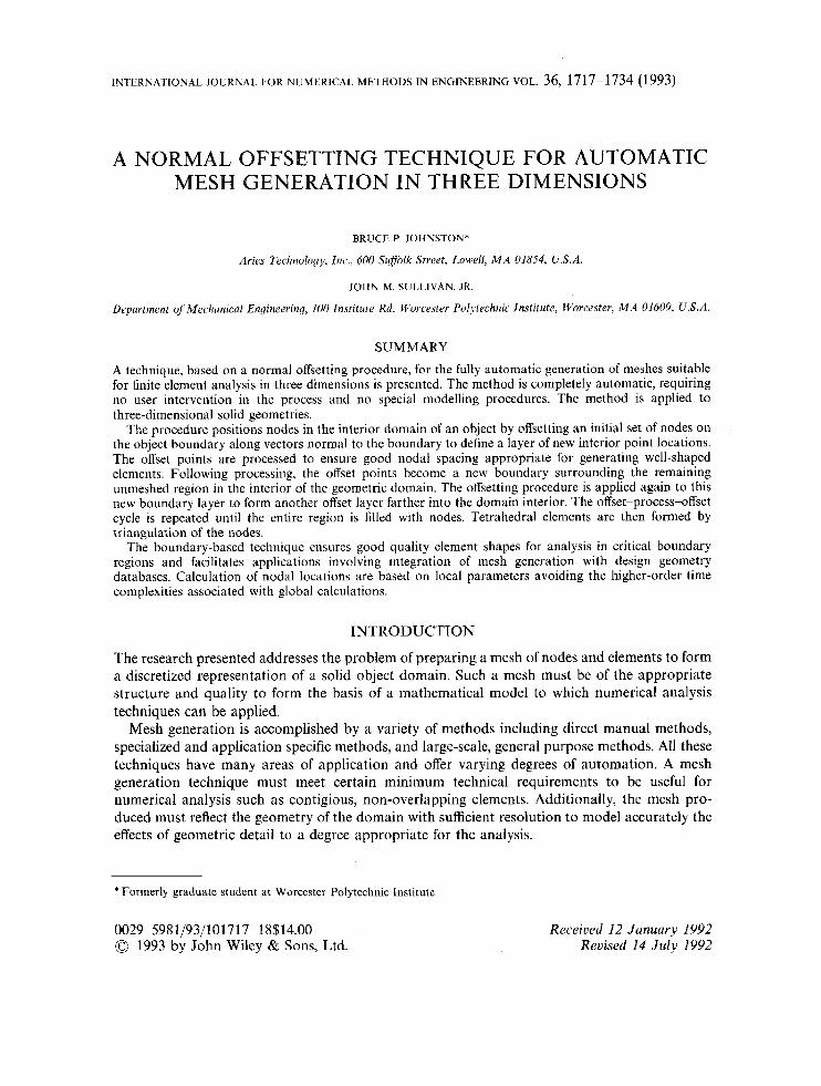
In general, the shape of an offset layer is not the same as that of its parent layer or of the original boundary. Offsetting points along vectors normal to curved boundaries causes conver- gence in concave regions and divergence in convex regions (Figure l(a)). This situation results in unacceptable nodal spacing and, consequently, a poor-quality mesh. Non-uniform mesh density requirements can cause an increase or decrease in the number of points in the new layer. In addition, offsetting highly concave geometries can cause sharp angles (Figure 2(a)), looping and self-intersection (Figure 2(b)) in the new layer which limit the layer's ability to serve as a parent for subsequent steps. To alleviate these conditions, the new layer of points is processed to determine final acceptable nodal locations. The resulting processed layer serves as a well-conditioned parent layer for the next step (Figures (lb), (lc), (2c) and (2d).

The processing required to maintain acceptable nodal spacing within an offset layer flows through a series of four checks: distance, angle, intersection and termination. Each iayer-process- ing check acts at the local level to ensure that a given node is in an acceptable location relative to its immediate neighbours. This approach avoids global comparisons (node against all preexisting nodes) and their associated higher-order time complexity. In addition, geometry at the local level remains quite simple, even for objects with very complex overall geometries. This simplicity

1720 R. P. JOHNSTON AND J. M. SULLIVAN JR.

I L i

Corner collapsed, 'Ti Connectivity

rerouted -

L i Li+l

Figure 2. Oftsetting a layer: (a) sharp corner; (b) overlap region; (c) sharp corner resolved; (dl overlap resolved

allows relatively simple local checks to control more complex global placement of nodes in the domain.

Once the domain is filled with acceptably spaced nodes, an element generation procedure is applied to form a continuous mesh of elements.

Boundary meshing

In order to initialize the three-dimensional offsetting process, an array of nodes on the boundary must exist. We use a pre-existing boundary surface mesh of linear triangles. The element connectivity becomes the facets of the initial boundary layer.

The exclusive use of the normal offsetting method to completely mesh three-dimensional solids is possible. In such an implementation, the boundary entities would be meshed by a two- dimensional implementation of the offsetting method in the parametric space of bounding surfaces.

AUTOMATIC MESH GENERATION 1721

Mesh density considerations

The ability to control the density and gradation of element sizes from one location within the domain to another is an important aspect of the mesh generation process. The normal offsetting technique incorporates mesh density information directly into the process by which nodal locations and, thus, element sizes, are determined. A global base element ske is first established for the entire domain prior to the initiation of mesh generation. This global element size represents the average element size that would result from a completely uniform discretization of the domain and is set prior to the initiation of the mesh generation process. Each offset calculation and processing check which is related to the size of a potential element uses an element size value obtained by modifying the global base value with a mesh density factor appropriate for the specific location in the domain. This inclusion of mesh density in the process eliminates the need for post-processing techniques such as element subdivision and mesh smoothing to enforce mesh density considerations.

In order to maintain a broad range of application for the method and close integration of mesh density in the offsetting process, the actual method for determining mesh density was decoupled from the mesh generator. The only requirement of the density function is that it return a scalar mesh density value for any arbitrary point in the domain.

Ofset calcula t ions

The calculation of the point locations associated with an offset layer requires three compon- ents: an initial layer of nodal locations, offset directions for each node and offset distances for each node. The initial locations are provided by the existing layer of nodes, L,, where i refers to the ith offset step. The offset direction at each node. N,, where j represents the jth location in a given layer, is defined as a vector, V,, normal to the existing layer at the nodal location (Figure l(a)). The normal value is calculated directly from the triangular facet connectivity of the parent layer as the average of the normals of all the facets attached to the given node:

where nadj is the number of adjacent facets. A simple in/out test determines if thc vector points in or out of the domain.

The offset distance along this normal vector is calculated from two components; the global base element size and the local mesh density value. The co-ordinates of the point in the new layer are calculated by moving along the parent’s normal vector, the offset distance. The mesh density value is checked at the new location. If this density value differs significantly from that of the parent the offset distance is recalculated until convergence, usually in one or two cyclcs.

Distance tolerance check

The distance between each point in the new layer and each adjacent point in the facet connectivity is checked against an upper and lower bound. These bounds are determined from the base element size, modified by the local mesh density to produce an ideal nodal spacing for a given pair of adjacent points. A lower bound of 67 per cent of the ideal spacing and an upper bound of 133 per cent of the ideal spacing work well in implementation. This results in tangential spacing of nodes falling within a range of f 33 per cent of the ideal values.

1722 B. P. JOHNSTON AND I. M. SULLIVAN JR.

Figure 3. Unacceptable nodal divergence corrected by edge swapping

a) b)

Figure 4. In-surface angle processing: (a) small in-surface angle; (b) angle removed by collapsing

Two points separated by a distance less than the lower bound are snapped together at their average co-ordinate and the two facets adjacent to the edge connecting the points are deleted from the surface connectivity. If two points are separated by more than the allowable (Figure 3(a)) spacing, a diagonal swap of the offending edge is attempted (Figure 3(b)). If this swapped edge is an acceptable length then the problem is resolved; otherwise, an additional point is inserted at the midpoint of the diagonals (Figure 3(c)).

Angle tolerance check

In general, there is an angle formed by each unique permutation of two edges connected to a point. These angles can be grouped into two categories. In-surface angles are formed by adjacent edge pairs and form the interior angles of the surface facets adjacent to the point (Figure 4(a)). Cross-surface angles are formed by non-adjacent edges and represent a measure of the ‘folding’ or ‘peaking’ of the surface (Figures 5(a) and 6(a)).

If the value of an in-surface angle falls below a minimum value, the two end points of the angle are snapped together (Figure 4(b)). An implemented value of 30” works well and represents a reasonable minimum interior angle for a tetrahedral element face.

Cross-surface angles measure ‘sharpness’ of the advancing surface layer in regions of concave curvature. When a cross-surface angle falls below a minimum value, the surface connectivity must

AUTOMATIC MESH GENERATION 1723

a) b)

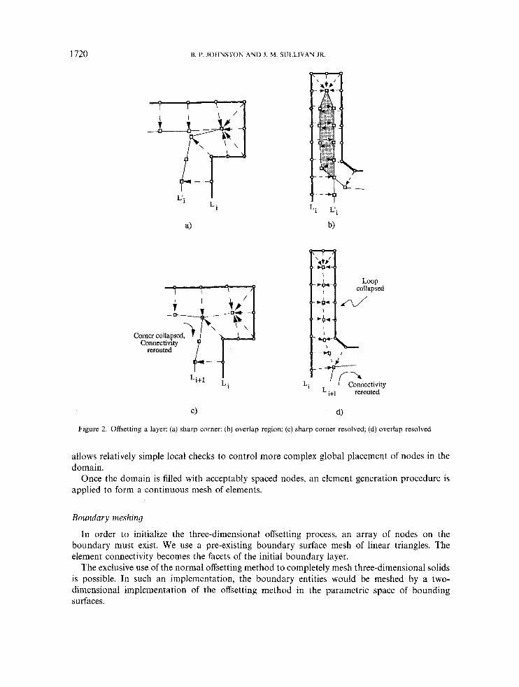
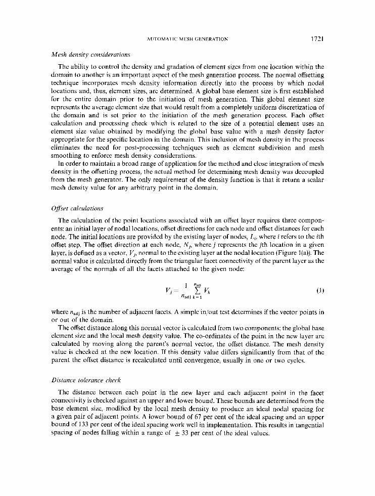
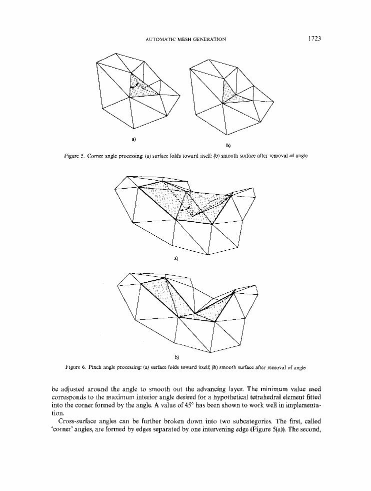
Figure 5. Corner angle processing: (a) surface folds toward itselt (b) smooth surface after removal of angle

a)

b) Figure 6. Pinch angle processing: (a) surface folds toward itself; (b) smooth surface after removal of angle

be adjusted around the angle to smooth out the advancing layer. The minimum value used corresponds to the maximum interior angle desired for a hypothetical tetrahedral element fitted into the corner formed by the angle. A value of 45" has been shown to work well in implementa- tion.

Cross-surface angles can be further broken down into two subcategories. The first, called 'corner' angles, are formed by edges separated by one intervening edge (Figure 5(a)). The second,

1724 B. P. JOHNSTON AND J. M. SULLIVAN JR.

a> b) c)

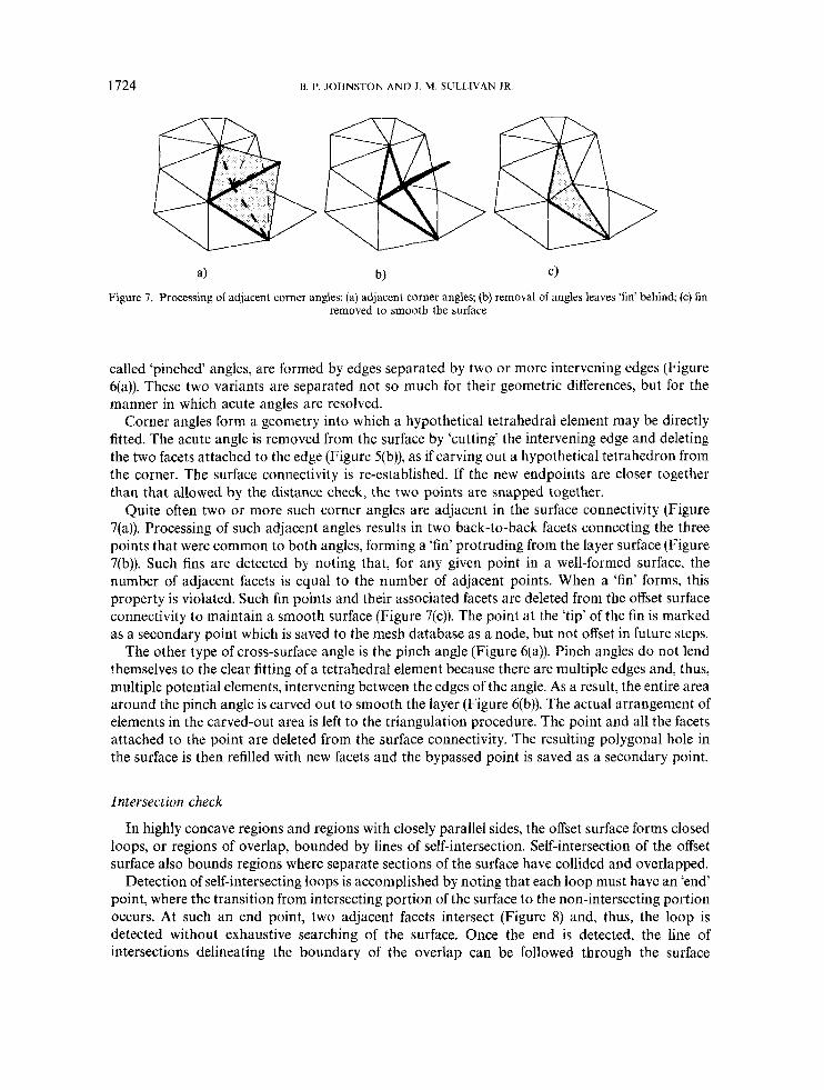
Figure 7. Processing of adjacent corner angles: (a) adjacent corner angles; (b) removal of angles leaves ‘fin’ behind (c) fin removed to smooth the surface

called ‘pinched’ angles, are formed by edges separated by two or more intervening edges (Figure 6(a)). These two variants are separated not so much for their geometric differences, but for the manner in which acute angles are resolved.

Corner angles form a geometry into which a hypothetical tetrahedral element may be directly fitted. The acute angle is removed from the surface by ‘cutting’ the intervening edge and deleting the two facets attached to the edge (Figure 5(b)), as if carving out a hypothetical tetrahedron from the corner. The surface connectivity is re-established. If the new endpoints are closer together than that allowed by the distance check, the two points are snapped together.

Quite often two or more such corner angles are adjacent in the surface connectivity (Figure 7(a)). Processing of such adjacent angles results in two back-to-back facets connecting the three points that were common to both angles, forming a ‘fin’ protruding from the layer surface (Figure 7(b)). Such fins are detected by noting that, for any given point in a well-formed surface, the number of adjacent facets is equal to the number of adjacent points. When a ‘fin’ forms, this property is violated. Such fin points and their associated facets are deleted from the offset surface connectivity to maintain a smooth surface (Figure 7(c)). The point at the ‘tip’ of the fin is marked as a secondary point which is saved to the mesh database as a node, but not offset in future steps.

The other type of cross-surface angle is the pinch angle (Figure 6(a)). Pinch angles do not lend themselves to the clear fitting of a tetrahedral element because there are multiple edges and, thus, multiple potential elements, intervening between the edges of the angle. As a result, the entire area around the pinch angle is carved out to smooth the layer (Figure 6(b)). The actual arrangement of elements in the carved-out area is left to the triangulation procedure. The point and all the facets attached to the point are deleted from the surface connectivity. The resulting polygonal hole in the surface is then refilled with new facets and the bypassed point is saved as a secondary point.

Intersection check

In highly concave regions and regions with closely parallel sides, the offset surface forms closed loops, or regions of overlap, bounded by lines of self-intersection. Self-intersection of the offset surface also bounds regions where separate sections of the surface have collided and overlapped.

Detection of self-intersecting loops is accomplished by noting that each loop must have an ‘end’ point, where the transition from intersecting portion of the surface to the non-intersecting portion occurs. At such an end point, two adjacent facets intersect (Figure 8) and, thus, the loop is detected without exhaustive searching of the surface. Once the end is detected, the line of intersections delineating the boundary of the overlap can be followed through the surface

AUTOMATIC MESH GENERATION 1725

et

Point of intersectio

intersection

Figure 8 Detection of loop and overlap ends

final location of offset point and opposite side

intersection of normal

\

- distance half way L i back to intersection

Figure 9. Resolution of overlaps by pulling surfaces back to ‘centrelines’

connectivity to cut off the overlap area. This will leave a polygonal hole in the surface connectivity which is subsequently refilled with new facets to bypass the loop points. The overlap region may then be collapsed by moving points back along their normals half-way to the point of intersection with the opposite side of the overlap (Figure 9). Points within a distance tolerance of the opposite side are deleted. The remaining set of points from both sides are ehecked against each other for proper spacing. Points which survive all the checks are marked as secondary points.

The second kind of intersection, the collision overlap, occurs when a ‘dome’ from one portion of the surface moves through an opposite region of the surface. Such an overlap is detected by checking the inlout status of each point. Once the bounds of the overlap are delineated, the region is removed and collapsed as with the loop. The remaining surface connectivity is reconnected to form a toroidal surface topology.

Surface division

A surface can be divided during the offsetting process. Division of the surface layer occurs whenever a triangular cross-section is collapsed. Such a collapse results in more than two facets

1726 B. P. JOHNSTON AND J. M. SULLIVAN JR.

Figure 10. Collapse of triangular cross-section results in splitting of surface: (a) snapping adjacent points collapses cross-section; (b) swapping of long edge collapses cross-section; (c) resulting collapsed edge; (d) surface split by deleting

facets connected to edge

being connected to an edge and is detected just as ‘fins’ were during angle processing. Triangular cross-sections are collapsed to create multi-connected edges when two of the cross-section points are snapped together (Figure 10(a)) or when reconnection of the surface connectivity closes off the cross-section with a new facet (Figure 10(b)). Both cases result in two distinct regions of the surface connected along a shared edge (Figure lO(c)).

The surface is divided into two isolated sections each with a polygonal hole in its connectivity. These holes are refilled with new facets using the same procedure used during processing of pinched angles (Figure 10(d)).

Many such divisions occur during the processing of general three-dimensional geometries. Quite often, such splits are associated with small knobs and fingers attached to the main surface and the new surface section formed consists of only a few points. Such mini-sections are usually immediately collapsed and deleted by further distance and angle checks. Sections that are not immediately collapsed form independent boundary layers surrounding distinct unmeshed regions of the domain. Further offsetting steps are performed independently on each section until each converges.

Termination criteria

Convergence is detected by checking the number of remaining points in each section of the surface following completion of all processing checks. If four or fewer points remain in a section then that section is terminated and the points are saved as nodes. This number of nodes must form an acceptable element geometry. Less than four points cannot form a closed region in three dimensions. If more than four points remain then the volume is checked.

Volume is calculated using a Gauss-Green formulation to derive the volume directly from the surface triangulation. The integral representation of the volume function may be transferred to a bounding surface by the relation

P I-

J y d x d y d r = xii,dS Js

AUTOMATIC MESH GENERATION 1727

where x is the x-component of a point on the surface, f ix is the x-component of the unit normal to the surface at the point and dS is the differential area around the point. For a surface made up of discrete flat facets, the integral expression may be rewritten as a summation of the integrals for each facets:

N

(3)

Furthermore, the normal vector will remain constant for any given facet and may, thus, be removed from the integral:

N xii,dS = i = 1 1 fix,[s,xidSi

The remaining integral can be evaluated using triangular area

and, thus, Xi = lIX1 + 12x2 + 13x3

JsidSi = jS,(l1x1 + Z2x2 + 13~3)dSi

= ls , l lxldSi + js,12x2dSi + = 4x1’4 + $xzA + 3 X 3 A

Volume can now be determined by N

v = c ii,,&(x, + x2 + X J ) i = 1

(4)

co-ordinates so that

Equation (6) yields a value for volume which will be positive if all the surface normals point outward and will be negative if the surface normals point inward. A negative value for volume indicates that the boundary surface has completely overlapped and inverted. Sections with such negative volumes are terminated and their points processed as an overlap region.

Speciul considerations

Multiconnected boundaries in three dimensions are used to represent hollow objects. If the meshing of such hollow objects is desired then multiple surface sections, as implemented with respect to splitting of the surface during processing, may be used to represent the boundaries of such isolated pockets in the interior of the domain. Normal directions associated with points of such an interior region point outward into the object domain. Calculations and processes associated with interior layer points are identical to those associated with points on exterior layers since at the local level both geometries are identical. Collisions between the different layer sections are detected in the same manner as collisions between opposing portions of a single section. Two colliding interior sections are merged into one larger interior section which continues to advance outward. When an interior section collides with an exterior layer, the interior section is absorbed into the exterior layer which continues to advance ‘inward’ into the unmeshed domain.

Multiple materials within the domain of a single object can also be implemented as multicon- nected boundaries. In this case, each material region represents a closed domain unto itself, with

1728 R P JOHNSTON AND J M SULLIVAN JR

its own distinct boundary but sharing the geometric entities which form common boundaries with other material regions. Individual materials may have multiconnected boundaries, thus allowing one material to be completely enclosed by another. Even with such nesting, however, nodes from one material region will never be offset into a neighbouring region of another material and, thus, intersection between advancing layers of differing materials need not be considered.

Element generation

Elements are generated from the nodal array using Watson’s method4 to produce the three- dimensional Delaunay triangulation. The three-dimensional Delaunay triangulation is not an optimum discreti~ation from the standpoint of finite element analysis and has been known to produce a significant number of degenerate elements in reported implementations. Cavendish’, for example, reports Delaunay triangulations containing up to 10 per cent degenerate elements. These degenerate elements are, however, significantly reduced in number or eliminated by the nodes produced by our nodal offsetting method. This improved nodal spacing produced by normal offsetting results in triangulations, without any post-processing, which generally contain less than 1 per cent degenerate elements, the maximum percentage encountered to date being 1.7 per cent.

Evaluation of time complexity

The time complexities for each of the majors steps of the normal offsetting process are summarized in Table I.

The number of boundary nodes can be used to determine an upper bound on an operation since the number of nodes in each successive layer decreases, on an average, with each offsetting advance of the layer. Locally convex geometries with high mesh density in the convex regions might result in a temporary increase in the number of nodes when an individual layer is offset, but the overall trend in the number of nodes per layer remains downward over a number of steps.

Since time complexity is governed by the highest order of each sequential phase, the overall time complexity for the processing of each layer is O(n2) and is governed by the intersection checking process. Mesh density function evaluation will generally have low time complexity but is ultimately dependent upon the function used and its implementation.

The overall time complexity for the process can be determined by considering the number of offsets required to fill an area. This in turn is related to the ratio of the object surface area to the distance between the boundary and the last layer. The worst case for determining the number of offsets required is the sphere. In this case, the ratio is given by

Since the number of steps to convergence is related to radius, r, and the number of boundary nodes is related to area, A, equation (7) can be rewritten as

Thus, the number of steps required to converge is related to the square root of the number of nodes in the boundary layer. The time complexity to generate a complete nodal array with uniform spacing is, therefore, determined by the product of (a:’*) steps with O(nz) operations per

AUTOMATIC MESH GENERATION 1729

Table I. Time complexity for the component steps in normal offsetting

Process Complexity Upper bound

Boundary geometry meshing Oinb) O(n,) Layer offsetting calculations W,) o(nb)

Distance tolerance checking 0 ( I $ . ) o(nb) Angle tolerance checking OinJ Oinb) Intersection checking O ( n 3 O(n3

implementation-dependent) W,,) 0(n,,) Mesh density evaluation

nb = number of nodes on the boundary n , = number of points in current layer nmd = number of points in mesh density function

step, which yields O(n,5'7 for the complete offsetting process. It is more common, however, to present mesh generation time complexity in terms of the total number of nodes in the mesh, a,. The above expression may be converted from number of boundary nodes to total number of nodes by examining thc rclationship of thc surface arca to the volume o f the object. Again, for a sphere this relation is

For a given mesh density, the number of nodes on the boundary is proportional to the surface area (nb = k iA) and the total number of nodes is proportional to the domain volume (n, = kz Y ) . Thus, the above expression may be rewritten in terms of nb and n, as

Thus, the Ofn;") time complexity becomes nodes, n,, for the three-dimensional implementation of the nodal offsetting process.

time complexity in terms of total number of

EXAMPLES

Several examples illustrate the three-dimensional implementation of the method. Figures of three-dimensional offset surfaces are presented in hidden line form for clarity. Numerical evalu- ation of the quality of the final meshes using the aspect ratio 4, defined as the ratio of the radius of inscribed sphere to radius of circumscribed sphere, is provided in place of tetrahedral figures to aid in evaluating the success of the method.6 An ideal, equilateral tetrahedron will have an ci value of 0.333. An element with an d value less than 0.01 is considered degenerate and invalid for use in analysis. Little published data are available detailing mesh quality produced by other mesh generation methods. Buratynski' reports average ci values of 0.224 and 0.225 for two examples with a minimum value of 003. Cavendishs reports meshes with up to 10 per cent of elements with Li values less than 0.01.

The first example is a cubic domain with a slender appendage attached. The initial boundary mesh was generated using the ANSYS' finite element program. Figure l l(a) shows the initial boundary surface representation. This surface is then offset as shown in Figure 1 l(b). Note how

1730 €3. P JOHNSTON AND J. M. SULLIVAN JR.

f)

Figure 11. Example 1: (a) initial boundary surface; (b) initial offset step; (c) first offset step after processing; (d) second offset step; (e, surface split during processing of second step: (f) second step after processing; (g) third (final) offset step after

processing.

the edges of the cube and finger have overlapped. Note also how the point spacing has increased in the neck region of the appendage because of the convex geometry in that region. Figure 1 l(c) shows the result of the first offset step after processing in which all the overlaps have been eliminated and the nodal spacing restored. The second offset step initially produces the same overlapping along the cube’s edges as well as a complete overlap of the appendage (Figure 1 l(d)). During processing of this step, part of the appendage is split off to form a new section of the offset surface (Figure ll(e)) but is completely collapsed away by further processing. The final offset surface resulting from step 2 is shown in Figure l l ( f ) . A third offset step produces the surface shown in Figure ll(g). A fourth step produced a completely overlapped surface resulting in termination of the process without further processing. Table I1 shows the breakdown of the elements by their ri values. Only 0.17 per cent of the elements fall into the degenerate category.

The second example is a domain representing a human torso used in hyperthermia analysis.’ The boundary meshed in this example was constructed by digitizing nodes from cross-sectional computer-aided tomography (CAT) images (Figure 12(a)). This model represents an example of

AUTOMATIC MESH GENERATION 1731

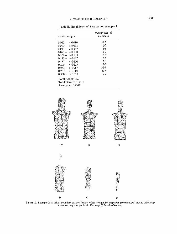
Table 11. Breakdown of i values for example 1

ii ratio ranges Percentage of

elements

0.000 ~ > 0.010 0.010 - > 0.033 0.033 - > 0-067 0'067 - > 0.100 0.100 - > 0.133

0.167 - > 0.200 0.200 ~ > 0.233 0.233 ~ > 0.267 0.267 - > 0,300

0.133 - > 0.167

0-300 - > 0.333

Total nodes: 762 Total elements: 3610 Average Ci: 0,2398

0.2 1.0 1.6 2.0 2.8 3.3 7.0

12.3 336 27.3 9.9

d) e) 0 Figure 12. Example 2 (a) initial boundary surface; (b) first offset step; (c) first step after processing; (d) second offset step

forms two regions; (e) third offset step; (f) fourth offset step

I732 B. P. JOHNSTON AND J . M. SULLIVAN J R

Table 111. Breakdown of ri values for example 2

Percentage of ri ratio ranges elements

0.000 - > 0.010 0.010 - > 0.033 0.033 - > 0.067 0.067 - > 0,100 0.100 - > 0-133 0.133 - > e l 6 7 0.167 - > 0.200 0.200 - > 0.233 0.233 - > 0.267 0.267 - > 0'300 0300- >0.333

Total nodes: 2193 Total elements: 1 I 619 Average 13: 0.2260

1 .o 2.1 1.9 2.8 3.6 4-2 7.0

15.4 34.7 21.8

5.4

Table IV. Breakdown of ri values for example 3

Percentage of % ratio ranges elements

0.000 - > 0.010 0.010 - > 0.033 0-033 - > 0067 0.067 - > 0.100 0.100 - > 0133 0.133 - > 0.167 0.167- >0200 0.200 ~ > 0.233 0.233 - > 0.267 0-267 - > 0.300 0.300 - > 0'333

Total nodes: 4221 Total elements: 21 952

1.2 0.5 1.7 1-7 3.4 5.3 8.4

15.9 26.9 26.0 9.1

an arbitrarily curved boundary surface. The initial offsetting of this model produces an offset layer (Figure 12(b)) that appears very similar to its parent. Close examination, however, shows unacceptably increased nodal spacing in the concave neck region and unacceptably decreased spacing in the head. Processing of the layer corrects these problems to produce an acceptable final layer surface (Figure 12(c)). The result of the second step is that the surface has been split to form a separate closed section in the head region (Figure 12(d)). By the end of the next step, the head section has terminated (Figure 12(e)). The body section continues to advance inward in step four (Figure 12(f)) and finally terminates by complete overlap when a fifth step is attempted. Tri- angulation of the final nodal array yields 11619 tetrahedral elements. Table I11 shows the breakdown of these elements according to their d values. Only 1 per cent fall below the degenerate threshold.

AUTOMATIC MESH GENERATION 1733

a)

e)

Figure 13. Example 3: (a) initial boundary surface; (b) first offsetting step before processing; (c) result of distance check; (d) final surface after angle processing; (e) second offset step after processing (f) third offset step after processing

The final example is a model of a hypothetical metal forming die and represents an example of a realistic design geometry. The boundary model was generated at the Wyman Gordon Company for boundary element analysis using the SDRC-Ideas'' program (Figure 13(a)). The first offset- ting results in the overlap of the entire wall section along the back of the die and along most of the angular edges (Figure 13(b)) as well as much stretching and compression of the offset surface. Distance tolerance checking restores acceptable nodal spacing and, in the process, cleans up many of the small overlap areas (Figure 13(c)). The large terminal overlap along the two back edges, however, remains. Processing of the offset layer by the angle tolerance check succeeds in removing the entire overlap area by collapsing in from the terminal edges to produce the final offset layer of the first step (Figure 13(d)). The second step results in the entire bottom of the trough region overlapping and splitting the offset surface into two large regions (Figure 13(e)). The thin post region is also collapsed and removed. The third step results in further shrinkage of

1734 8. P. JOHNSTON AND J. M. SULLIVAN JR.

the two surface sections (Figure 13(f)). The third section, shown in the middle of Figure 13(f), is ar, overlapped section of the layer that was split off during processing and terminated. The remaining two regions terminate in the fourth step. Table Iv shows the breakdown of ci values for this mesh. Into the degenerate category, 1.2 per cent of the dements fall.

CONCLUSION

The normal offsetting method has been shown to be a badly applicable and efficient technique for the generation of high-quality meshes for numer1:al analysis in three dimensions. The technique follows a simple, logical process to produce array of nodes with a high degree of control over inter-nodal spacing and, thus, element size,density and gradation, without user interaction during the meshing process. This simplicity of he process allows the method to capable of generating meshes in a completely automatic mole because there are no ambiguous situations which require user intervention to resolve.

The exclusive use of boundary information to initiate the lrocess makes integration of the technique with design geometry systems a straightforward pf)cess. The need to reconstruct geometric domains with special purpose geometric models, or ad1 additional geometric descrip- tions exclusively for analysis modelling is eliminated.

The high-quality nodal array results in increased element quaity in the final mesh when compared to existing nodal connection methods. The local nature of he calculations used in the process allows the technique to be applied with equal success to a vide variety of geometric configurations and complexity.

The layered structure of the process and associated local nature of tht required comparisons and calculations results in overall time complexity of the process of O(n:’.) . This compares with the O($) complexities associated with global comparisons and calculations,

The technique is based on such dimensionless principles as domains, boundaries and direc- tions. No special consideration is needed to incorporate specific geometric features such as holes or material regions. The method is, therefore, possible to be implemented in both two and three dimensions with equal success.

ACKNOWLEDGEMENT

This work was sponsored in part by the National Institute of Health, Award No. 5 R01 CA3724.5-08.

REFERENCES

1. K. Ho-Le, ‘Finite element mesh generation methods: a review and classification’, Complet. Aided Des., 10, 27-38

2. B. P. Johnston and J. M. Sullivan Jr., ‘Fully automatic, two dimensional mesh generation using normal offsetting’, Int.

3. B. P. Johnston, ‘A normal offsetting technique for the fully automatic generation of meshes in two and three

4. D. F. Watson, ‘Computing the n-Dimensional delaunay tessellation with applications to Vornoi polytopes’, Comput.

5. J. C. Cavendish, D. A. Field and W. H. Frey, ‘An approach to automatic three-dimensional finite element mesh

6. F. Durrell, Solid Geometry, Charles E. Merrill, New York, 1904. 7. E. K. Buratynski, ‘A fully automatic three dimensional mesh generator for complex geometries’, Int. j . numer. methods

8 . ANSYS is a registered trademark of Swanson Analysis Systems, Inc., Houston, PA. 9. K. D. Paulsen, X. Jia and D. R. Lynch, ‘3D bioelectromagnetic computation on finite elements’, in P. Fleming (ed.),

(1988).

j . numer. methods eng., 33, 425-442 (1992).

dimensions’, Ph.D. Thesis, WTD-246, Worcester Polytechnic Institute, Worcester MA, 1991.

J . , 24, 167 (1981).

generation’, Int. j . numer. methods eng., 21, 329-347 (1985).

ang. , 30, 931-952 (1990).

Applied Comp. Electromagnetic Society, special issue on Bioelectromagnetic Computations, 1992, to appear. 10. Ideas and SDRC are registered trademarks of Structural Dynamics Research Corp., Troy, MI.