A Neural Network Approach for Modelling Non Linear Transfer Functions:

Application for Wind Retrieval from Spaceborne Scatterometer Data

by

S. THIRIA*, C. MEJIA*,** , F. BADRAN* and M. CREPON**

* CEDRIC, Conservatoire National des Arts et Métiers292 rue Saint Martin - 75003 PARIS

** Laboratoire d'Océanographie et de Climatologie (LODYC), T14, Université de PARIS 64 Place Jussieu - 75005 PARIS (FRANCE)

Abstract

The present paper shows that a wide class of complex transfer functions encountered in geophysics

can be efficiently modelled by the use of neural networks. Neural networks can approximate

numerical and non numerical transfer functions. They provide an optimum basis of non linear

functions allowing a uniform approximation of any continuous function. Neural networks can also

realize classification tasks. It is shown that the classifier mode is related to Bayes discriminant

functions which give the minimum error risk classification. This mode is useful to extract information

from an unknown process. The above properties are applied to the ERS1 simulated scatterometer data.

When compared to other methods one finds that neural networks solutions are the most skillful.

Contents

1 . INTRODUCTION. . . . . . . . . . . . . . . . . . . . . . . . . . . . . . . . . . . . . . . . . . . . . . . . . . . . . . . . . . . . . . . . . . . . . . . . . . . . . . . . . . . . . . 1

2 . THE GEOPHYSICAL PROBLEM . . . . . . . . . . . . . . . . . . . . . . . . . . . . . . . . . . . . . . . . . . . . . . . . . . . . . . . . . . . . . . . . . 2

2.1. BACKGROUND...........................................................................................................2

2.2. THE SIMULATED DATA...............................................................................................5

3 . NEURAL NETWORKS . . . . . . . . . . . . . . . . . . . . . . . . . . . . . . . . . . . . . . . . . . . . . . . . . . . . . . . . . . . . . . . . . . . . . . . . . . . . . . 6

3.1. PRELIMINARIES.........................................................................................................6

3.2. The Quasi-linear Multi-layered Networks (QMN)..............................................................7

3.3. TRANSFER FUNCTION APPROXIMATION USING QMN................................................9

3.4. HOW TO USE QMN CLASSIFIER PROPERTIES TO ANALYSE UNKNOWNNUMERICAL TRANSFER FUNCTIONS.......................................................................10

THE METHOD....................................................................................................103.5. NUMERICAL RESULTS.............................................................................13

Determination of the wind speed..................................................................14

Determination of the direction......................................................................16

Performances.............................................................................................19

4 . THE “NEURAL MACHINE” (NM). . . . . . . . . . . . . . . . . . . . . . . . . . . . . . . . . . . . . . . . . . . . . . . . . . . . . . . . . . . . . . . . .20

NUMERICAL RESULTS OF THE COMPLETE NEURAL MACHINE.................23

CONCLUSION . . . . . . . . . . . . . . . . . . . . . . . . . . . . . . . . . . . . . . . . . . . . . . . . . . . . . . . . . . . . . . . . . . . . . . . . . . . . . . . . . . . . . . . . . . . . . .25

Acknowledgments. . . . . . . . . . . . . . . . . . . . . . . . . . . . . . . . . . . . . . . . . . . . . . . . . . . . . . . . . . . . . . . . . . . . . . . . . . . . . . . . . . . . . . . . .27

APPENDICES. . . . . . . . . . . . . . . . . . . . . . . . . . . . . . . . . . . . . . . . . . . . . . . . . . . . . . . . . . . . . . . . . . . . . . . . . . . . . . . . . . . . . . . . . . . . . . .27

APPENDIX A...........................................................................................................................27QMN AND FUNCTION APPROXIMATION.............................................................27

APPENDIX B...........................................................................................................................28CLASSIFIER MODE AND BAYES DISCRIMINANT FUNCTIONS.............................28

APPENDIX C..........................................................................................................................30Accuracy of the approximation for the classifier mode............................................30

REFERENCES. . . . . . . . . . . . . . . . . . . . . . . . . . . . . . . . . . . . . . . . . . . . . . . . . . . . . . . . . . . . . . . . . . . . . . . . . . . . . . . . . . . . . . . . . . . . . .32

1

1. INTRODUCTION

Transfer functions are widely employed in physics. They are mainly used to relate measured

quantities to significant physical parameters under study. In many cases transfer functions cannot be

determined from theoretical considerations and have to be estimated from a data set. As an example

oceanographers and meteorologists expect to measure the sea surface wind by using spaceborne

radar. Theory predicts some relationship between the backscatter signal of the radar and the wind

vector but the complete problem is too complicated to solve. Experiments with airborne radars have

been used to determine a semi empirical relationship for the backscatter signal as a function of the

wind vector and of the incidence angle. But the determination of the wind vector from the radar signal

leads to a very difficult inverse problem. In the present paper we propose a general method to

determine such complex transfer functions empirically by using neural networks

Neural networks (henceforth NN) offer interesting possibilities for solving problems involving

transfer functions [Rumelhart, 1986; Lippmann, 1987]. First, NN are adaptative providing a flexible

and easy way of modelling a large variety of physical phenomena. Here, adaptive means the ability of

the method to process a large number of data or to deal with new relevant variables Secondly, even if

the learning (or calibration) phase of the network takes a long time, the operational phase is very

efficient. This phase requires few calculations and can be carried out on small-sized computers.

Moreover NN architecture is easily implemented on dedicated hardware using parallel algorithms, thus

further reducing the processing time.

The aim of the present paper is first to show that NN are able to model a large class of complex

transfer functions and secondly to give a theoretical framework for the use of NN in that context. In

order to be as clear as possible we have chosen to deal with a particular example that demonstrates

several different possibilities of NN.

In what follows, attention is focused on the retrieval of scatterometer winds by the use of Neural

Networks. The method is presented in detail and can easily be extended to a large class of problems

involving the computation of empirical transfer functions. The matter is of interest since the European

satellite ERS1 with the AMI (Advanced Microwave Imager which can function in scatterometer mode)

was launched in 1991 and the American scatterometer NSCAT (NASA SCATterometer) should be

launched in 1996 on the Japanese satellite ADEOS. We have previously used NN to solve the

scatterometer wind ambiguity removal problem [Badran et al., 1991]. In the present work the

scatterometer wind retrieval and ambiguity removal are integrated in a complete Neural Machine (NM)

dedicated to computing horizontally consistent wind vectors from scatterometer backscatter

measurements.

2

First an analysis of the physical problem is presented and its possible decomposition into

different sub-problems is shown. The second section gives an overall presentation of NN and

describes in detail how they have been used in this work. Some theoretical results are provided in

order to offer a general method for approximating transfer functions; then some results using

simulated data are presented. The third section presents the "Neural Machine" and displays the

obtained results. Appendices give a deeper insight into the theoretical results.

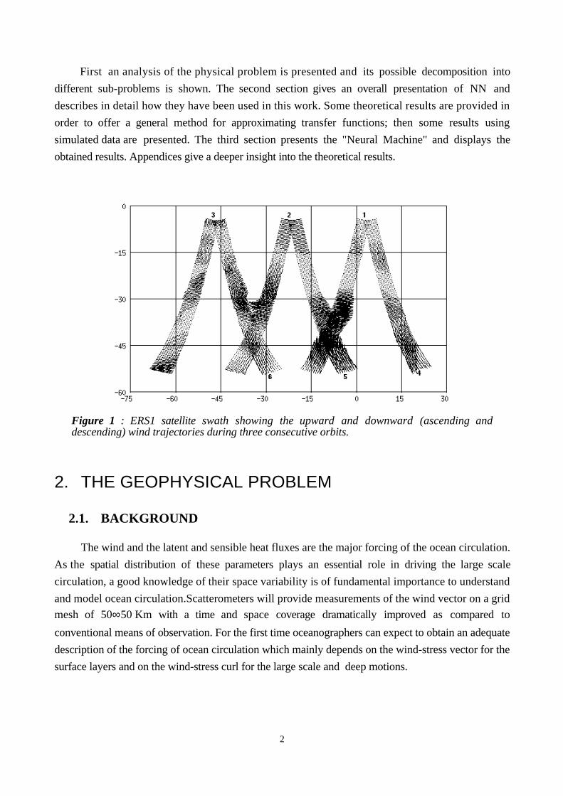
Figure 1 : ERS1 satellite swath showing the upward and downward (ascending anddescending) wind trajectories during three consecutive orbits.

2. THE GEOPHYSICAL PROBLEM

2.1. BACKGROUND

The wind and the latent and sensible heat fluxes are the major forcing of the ocean circulation.

As the spatial distribution of these parameters plays an essential role in driving the large scale

circulation, a good knowledge of their space variability is of fundamental importance to understand

and model ocean circulation.Scatterometers will provide measurements of the wind vector on a grid

mesh of 50∞50 Km with a time and space coverage dramatically improved as compared to

conventional means of observation. For the first time oceanographers can expect to obtain an adequate

description of the forcing of ocean circulation which mainly depends on the wind-stress vector for the

surface layers and on the wind-stress curl for the large scale and deep motions.

3

Scatterometers are active microwave radar which accurately measure the ratio of transmitted

versus backscattered power signal, a ratio usually called the normalized radar cross section (σ0) of the

ocean surface.The physics of the interaction of the radar beam with a rough sea-surface is poorly

understood. Such effects as wave breaking, modulation by long waves, and the effects of rain, make

the problem complex.

1i

n

antenna 1antenna 2

Satellite trajectories

swath

wind

antenna 3

sate

llite

traj

ecto

ry

wind

direction

2,i

forward beam

lateral beam

backward beam

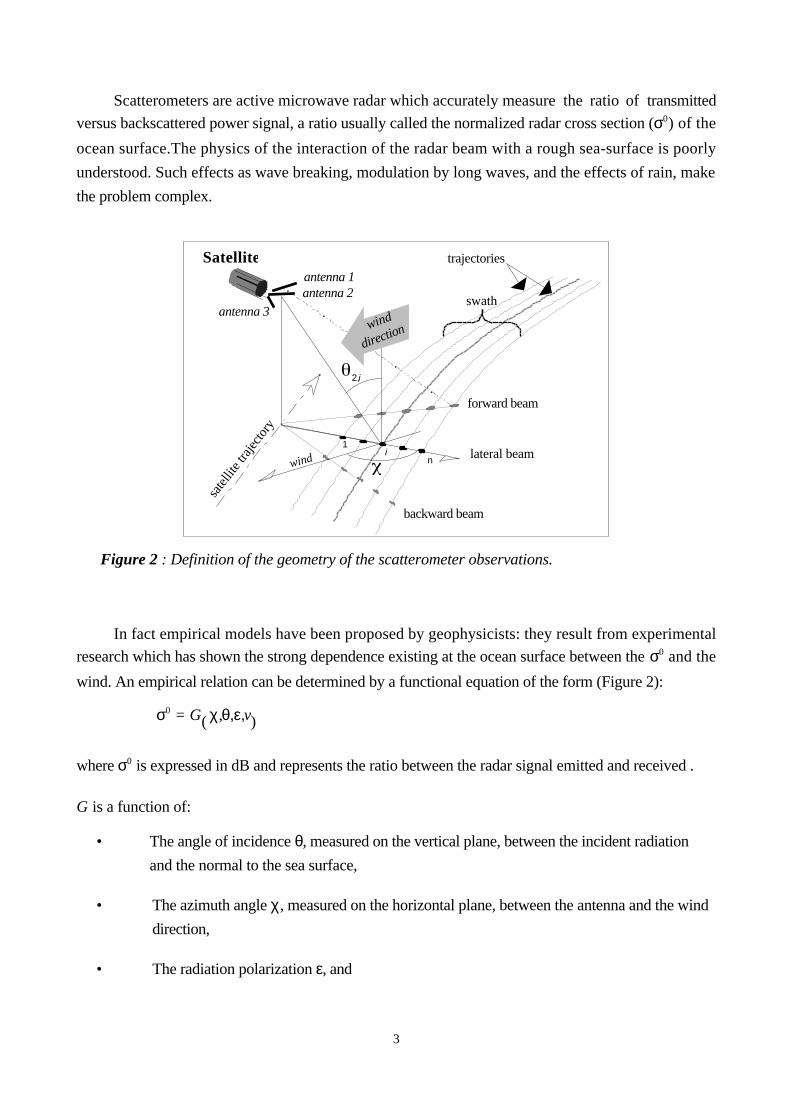
Figure 2 : Definition of the geometry of the scatterometer observations.

In fact empirical models have been proposed by geophysicists: they result from experimental

research which has shown the strong dependence existing at the ocean surface between the σ0 and the

wind. An empirical relation can be determined by a functional equation of the form (Figure 2):

σ0 = G( )χ,θ,ε,v

where σ0 is expressed in dB and represents the ratio between the radar signal emitted and received .

G is a function of:

• The angle of incidence θ, measured on the vertical plane, between the incident radiation

and the normal to the sea surface,

• The azimuth angle χ, measured on the horizontal plane, between the antenna and the wind

direction,

• The radiation polarization ε, and

4

• The wind speed v.

Since it is found that the σ0 varies harmonically with χ it is possible to compute the wind

direction by using several antennas pointing in different orientations with respect to the satellite track

(Price, 1976 - Freilich and Chelton, 1986).

A model developed by A. Long [Long, 1986] gives an expression for σ0 which is approximated by a

Fourier series of the form:

σ0 = U.

1 + b1

.cos( )χ + b2.cos( )2χ

1 + b1 + b2

with U = A.vγ

The parameters A and γ only depend on the incidence angle θ, b1 and b2 are a function of both the

wind speed v and the incidence angle θ.The different parameters used in this model are determined

experimentally.

The computation of the wind vector requires the inversion of the above formula

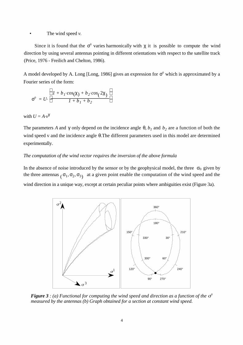
In the absence of noise introduced by the sensor or by the geophysical model, the three σ0 given bythe three antennas ( )σ1, σ2, σ3 at a given point enable the computation of the wind speed and the

wind direction in a unique way, except at certain peculiar points where ambiguities exist (Figure 3a).

360°

180°

210°

240°

270°90°

120°

150°

330°

300° 60°

30°

3

2

1

Figure 3 : (a) Functional for computing the wind speed and direction as a function of the 0

measured by the antennas (b) Graph obtained for a section at constant wind speed.

5

In the σ0 space, the graph of the above function (Figure 3a) is a triple cone-like surface with

singularities corresponding to ambiguities in the wind direction (Cavanié and Offiler, 1988 - Roquet

and Ratier, 1988). The directrix is a Lissajous curve which is a function of the wind direction whereas

a coordinate along the generatrix is a function of the wind speed. At a constant wind speed, theLissajous curve implies that two directions differing by 150° are possible for some ( )σ1, σ2, σ3

measurements (Figure 3b).

The problem is therefore how to retrieve wind vectors using the observed measurements

( )1 , 2 , 3 .

The determination of the wind vector may be decomposed into two different problems which are not

of the same order of difficulty. Due to the Lissajous ambiguities, computing the wind speed is easier

than computing the wind direction. Thus the whole problem can be decomposed into two sub-

problems leading to the determination of two distinct transfer functions. The first one is a singlevalued

function which permits the computation of the wind speed while the wind direction determination is a

multivalued function. The aim of this preliminary study is to show that neural networks can efficiently

solve such problems. The demonstration was made using simulated data and the results compared

with of more traditional methods. We now present the data set used for the experimental part of the

study.

2.2. THE SIMULATED DATA

As real data were not yet available, we have tested the method on simulated data computed from

meteorological models. The swaths of the scatterometer ERS1 were created by simulating a satellite

flying on wind fields provided by the ECMWF analysed output (Figure 1). The wind data werecollocated to the simulated satellite measurements. The backscatter values ( )σ1, σ2, σ3 given by the

three antennas were calculated using Long's model. Noise was then added to the σ0 in order to

simulate the errors made by the scatterometer and the small scale structures of the wind field (A

gaussian noise of zero average and of standard deviation 9.5% for both lateral antennas and 8.7%

for the central antenna was added at each measurement - see Appendix C). By way of comparison

the actual instrument noise of the ERS1 scatt is about 5%. Thus our simulations take into account

more than just instrument noise.

The data set used to calibrate the NN (the so-called learning set) was extracted from 22 maps

(Figure 1) representing 22 days of satellite observation over the southern Atlantic ocean, regularly

distributed over September 1986; the 9 days left were used to make the test. Results have been

tested on a data set of 5041 wind vectors. These wind data are error free.

6

The statistics performed on the learning set showed that the winds have a velocity ranging from 4 to

20 m/s with an average of 8.24 m/s and a standard deviation of 3.03 m/s. As the directions become

insignificant when the wind velocity is too weak, small amplitude winds (less than 3 m/s) were

eliminated.

The learning sets must be choosen in relation to specific goals. Thus two different learning sets

have been selected. The first one was selected in order to be statistically representative of the wind

speed, and the second of the directions. This operation is fundamental to ensure the accuracy of the

method. NN can be considered as statistical estimators and can only compute significant parameters

when they are calibrated by using statistically significant learning sets. The first results obtained

showed that some relation exists between the learning set's structure and the method's

performances: in fact under-represented speed or direction could not be computed correctly.

In order to get realistic results when the network is operating and to check its generalization ability, the

9 maps used during the test were not used at all during the learning phase.

In the following it is shown that neural networks have theoretical properties which allow them to

approximate complex transfer functions accurately. Section 3 is devoted to the approximation of

transfer function through the use of neural networks. Section 4 presents the NM which solves the

scatterometer remote sensing problem described above.

3. NEURAL NETWORKS

3.1. PRELIMINARIES

This section presents a basic discussion of Quasi-Linear Neural Network (QMN) which are the NN

used in the present work; a more complete presentation is available in [Badran, 1991] and reviews on

this technique are in [Rumelhart, 1986; Lippmann, 1987].

A neuron (or automaton) is an elementary transfer function which provides an output s (s [S)when an

input A is applied.

s = f(A)

f is the transition function.

An neural network is a set of interconnected neurons (Fig. 5). Each neuron receives and sends

signals only from the neurons to which it is connected (Fig. 4a). Thanks to this association of

7

elementary tasks a neural network is able to solve very complicated problems. This ability is related to

the number of neurons and to the topology of their connections.

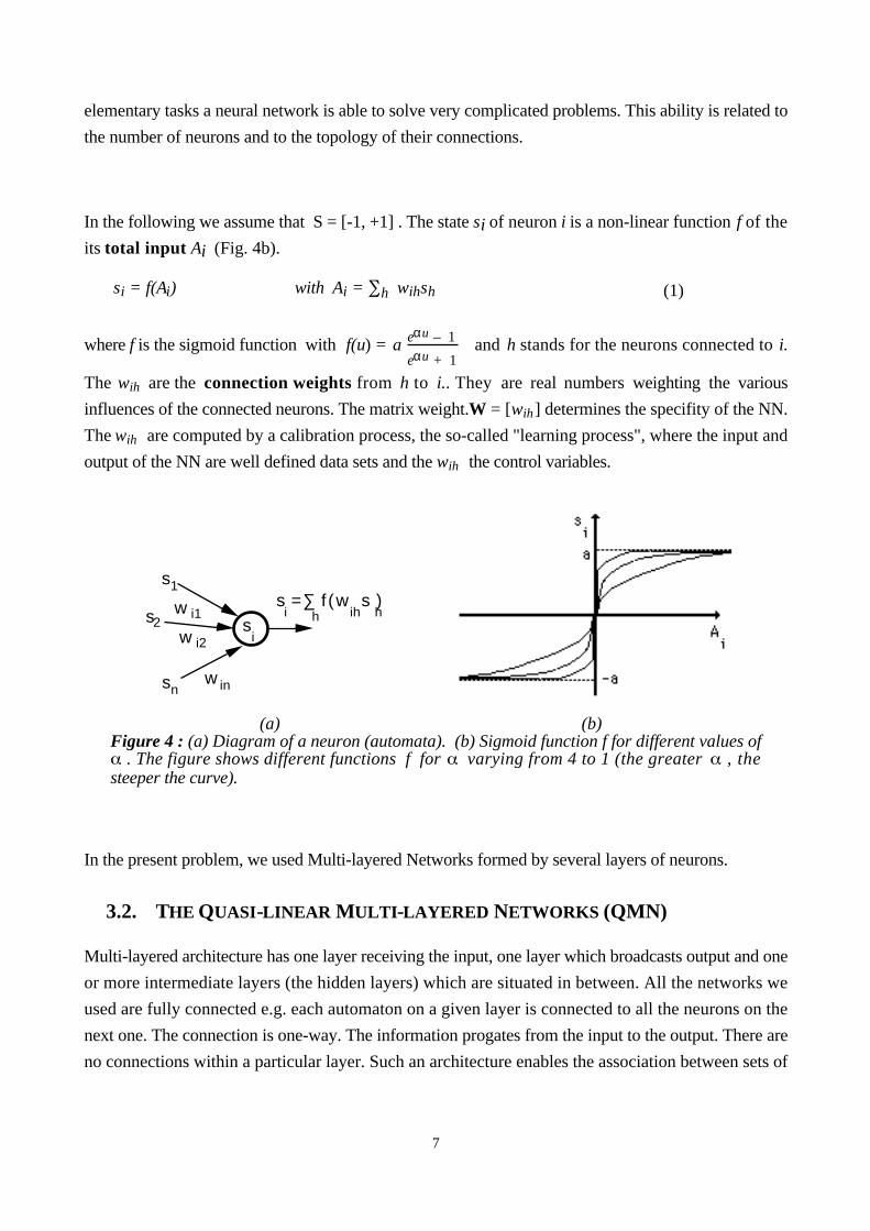
In the following we assume that S = [-1, +1] . The state si of neuron i is a non-linear function f of the

its total input Ai (Fig. 4b).

si = f(Ai) with Ai = h wihsh (1)

where f is the sigmoid function with f(u) = a eαu – 1

eαu + 1 and h stands for the neurons connected to i.

The wih are the connection weights from h to i.. They are real numbers weighting the various

influences of the connected neurons. The matrix weight.W = [wih] determines the specifity of the NN.

The wih are computed by a calibration process, the so-called "learning process", where the input and

output of the NN are well defined data sets and the wih the control variables.

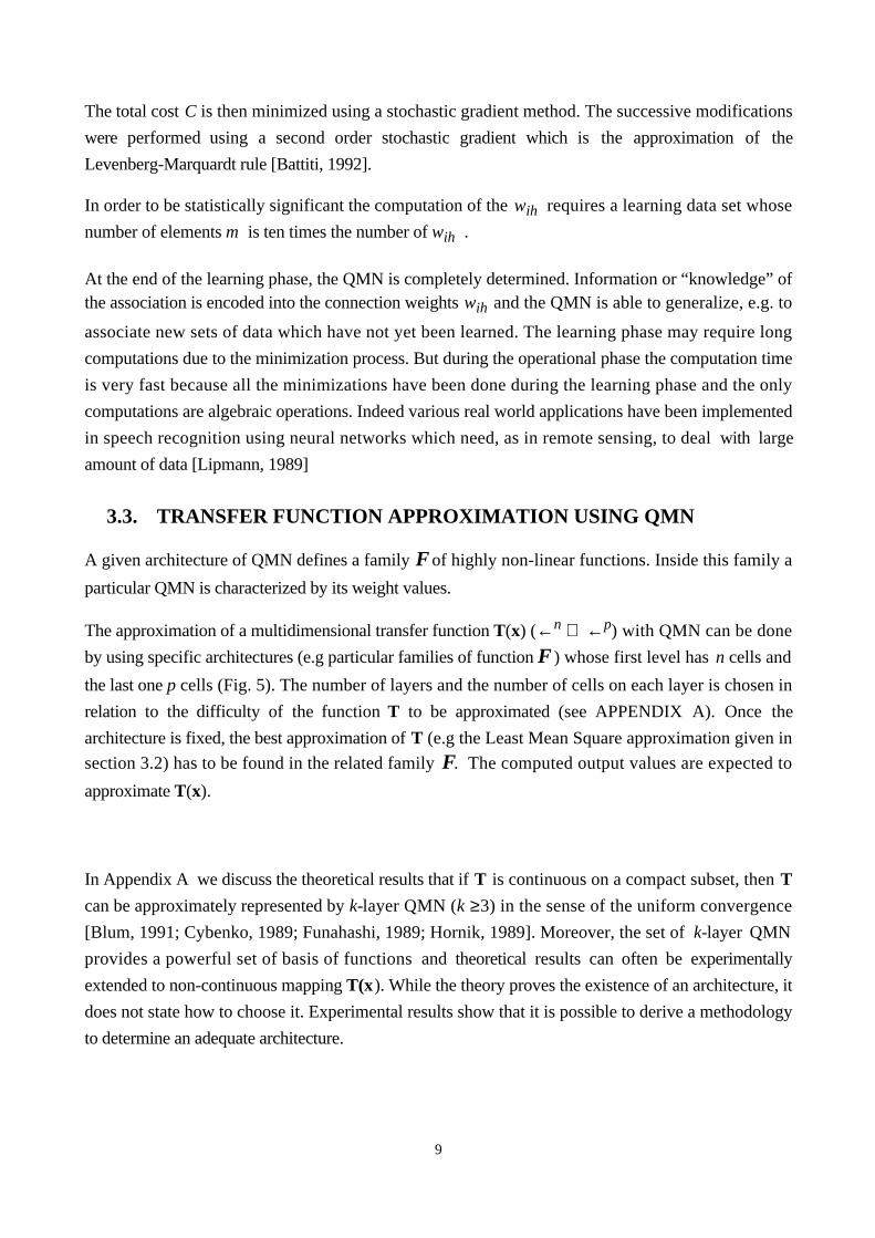
s1

s2

sn

si

s =∑ f(w s )i h hihw i1

w i2

w in

(a) (b)Figure 4 : (a) Diagram of a neuron (automata). (b) Sigmoid function f for different values of

. The figure shows different functions f for varying from 4 to 1 (the greater , thesteeper the curve).

In the present problem, we used Multi-layered Networks formed by several layers of neurons.

3.2. THE QUASI-LINEAR MULTI-LAYERED NETWORKS (QMN)

Multi-layered architecture has one layer receiving the input, one layer which broadcasts output and one

or more intermediate layers (the hidden layers) which are situated in between. All the networks we

used are fully connected e.g. each automaton on a given layer is connected to all the neurons on the

next one. The connection is one-way. The information progates from the input to the output. There are

no connections within a particular layer. Such an architecture enables the association between sets of

8

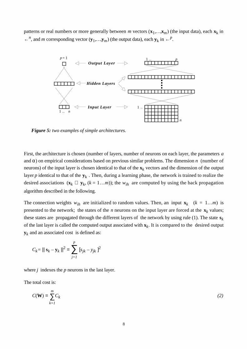
patterns or real numbers or more generally between m vectors (x1,…,xm) (the input data), each xk in

←n, and m corresponding vector (y1,…,ym) (the output data), each yk in ←p.

Output Layer

Hidden Layers

Input Layer

1 ... p

1 ...

n

1 ... n

p = 1

Figure 5: two examples of simple architectures.

First, the architecture is chosen (number of layers, number of neurons on each layer, the parameters a

and α) on empirical considerations based on previous similar problems. The dimension n (number of

neurons) of the input layer is chosen identical to that of the xk vectors and the dimension of the output

layer p identical to that of the yk . Then, during a learning phase, the network is trained to realize the

desired associations (xk ∅ yk, (k = 1…m)); the wih are computed by using the back propagation

algorithm described in the following.

The connection weights wih are initialized to random values. Then, an input xk (k = 1…m) is

presented to the network; the states of the n neurons on the input layer are forced at the xk values;

these states are propagated through the different layers of the network by using rule (1). The state sk

of the last layer is called the computed output associated with xk. It is compared to the desired output

yk and an associated cost is defined as:

Ck= || sk – yk ||2 = ∑

j=1

p

[sjk – yjk ]2

where j indexes the p neurons in the last layer.

The total cost is:

C(W) = ∑k=1

mCk (2)

9

The total cost C is then minimized using a stochastic gradient method. The successive modifications

were performed using a second order stochastic gradient which is the approximation of the

Levenberg-Marquardt rule [Battiti, 1992].

In order to be statistically significant the computation of the wih requires a learning data set whose

number of elements m is ten times the number of wih .

At the end of the learning phase, the QMN is completely determined. Information or “knowledge” ofthe association is encoded into the connection weights wih and the QMN is able to generalize, e.g. to

associate new sets of data which have not yet been learned. The learning phase may require long

computations due to the minimization process. But during the operational phase the computation time

is very fast because all the minimizations have been done during the learning phase and the only

computations are algebraic operations. Indeed various real world applications have been implemented

in speech recognition using neural networks which need, as in remote sensing, to deal with large

amount of data [Lipmann, 1989]

3.3. TRANSFER FUNCTION APPROXIMATION USING QMN

A given architecture of QMN defines a family F of highly non-linear functions. Inside this family a

particular QMN is characterized by its weight values.

The approximation of a multidimensional transfer function T(x) (←n ∅ ←p) with QMN can be done

by using specific architectures (e.g particular families of function F ) whose first level has n cells and

the last one p cells (Fig. 5). The number of layers and the number of cells on each layer is chosen in

relation to the difficulty of the function T to be approximated (see APPENDIX A). Once the

architecture is fixed, the best approximation of T (e.g the Least Mean Square approximation given in

section 3.2) has to be found in the related family F. The computed output values are expected to

approximate T(x).

In Appendix A we discuss the theoretical results that if T is continuous on a compact subset, then T

can be approximately represented by k-layer QMN (k ≥3) in the sense of the uniform convergence

[Blum, 1991; Cybenko, 1989; Funahashi, 1989; Hornik, 1989]. Moreover, the set of k-layer QMN

provides a powerful set of basis of functions and theoretical results can often be experimentally

extended to non-continuous mapping T(x). While the theory proves the existence of an architecture, it

does not state how to choose it. Experimental results show that it is possible to derive a methodology

to determine an adequate architecture.

10

3.4. HOW TO USE QMN CLASSIFIER PROPERTIES TO ANALYSEUNKNOWN NUMERICAL TRANSFER FUNCTIONS

One is often able to get measurements of a given phenomenon, but it is quite impossible to insert it in

a conceptual framework. So it is of interest to extract some information embedded in the data: this

could be the relevance of a given variable, information on the complexity of the phenomenon or the

derivation of an analytical transfer function modelling it.

We have seen that QMN are able to approximate transfer functions. The simplest transfer functions

we could imagine are numerical ones; a set of real vectors considered as input vectors are associated to

another set considered as output vectors. QMN are well suited to model such functions even if they

are non linear. QMN are also able to perform more complex even non numerical tasks.

In this section we present a methodology based on the latter QMN properties in order to get additional

information on the complexity of the unknown transfer function. In fact the interpretation of the

QMN outputs enables us to compute discrete values for T(x) with their related coefficients of

likelihood [Bourlard, 1990]. This is necessary when studying complex multi-valued transfer functions

which operate in a noisy environment. In that case, and for specific values of x, T(x) may have several

possible values and thus it is inadequate to compute just one value for T(x). When dealing with

scatterometer wind vector retieval the determination of the wind direction leads to such a problem. The

problem is solved by determining the different possible values with their coefficients of likelihood.

In the following a method to compute the different values and their coefficients of likelihood is

presented. The results obtained when using this method for the determination of the wind speed and

the wind direction measured by satellite scatterometers are then discussed. More details about

theoretical results and the generality of the approach are given in Appendix B and C [Gish, 1990;

Geman, 1992, White 1989].

THE METHOD

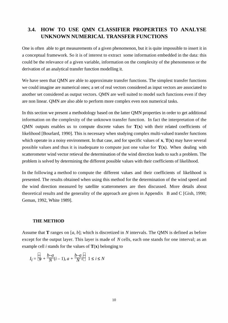
Assume that T ranges on [a, b]; which is discretized in N intervals. The QMN is defined as before

except for the output layer. This layer is made of N cells, each one stands for one interval; as an

example cell i stands for the values of T(x) belonging to

Ii =

a + b–aN (i – 1), a +

b–aN i 1 ≤ i ≤ N

11

network output discretized in N intervals

hidden layers

input layer

Figure 6 : the figure represents a N output network for the discretizd approach

An input pattern x is associated with class i if T(x) belongs to Ii. Approximating T(x) is now to learn

the association {(x,i), x in ←n}.

In order to associate a numerical value approximating T(x) we identify Ii by means of the centroid mi

e.g mi = a + b–aN i –

12

stands for Ii

We now have to define the desired output. For a given input x, the desired output vector y = (y1, y2, …,

yN) is coded by yi = +1 if the value of T(x) is in interval Ii and yi = –1 if not.

For a given weight matrix W, the QMN now approximates T using a function F(·,W) from

(←n ∅ ←N) N being the number of intervals used to discretize T. The output associated to vector x isa vector y of dimensionality N defined by: (F1(x,W), ...., FN(x,W)). The process to determine the

optimal mapping is the same as explained above:

Determination of the desired output T(x) = y

Computation of the network output F(x,W)

Minimization of the distance C(W) to get the Matrix W where

C( )W = ∑k=1

m

| |F(xk,W) – yk2 = ∑

k=1

m

∑i=1

N

( )Fi (xk,W) – yki 2

12

The QMN is now used as a classifier system. Theoretical results [Devijver, 1982; Duda, 1973;

White, 1989] allow us to compare the optimal mapping F(x,W*) computed by the back-propagation

algorithm (W* are the optimum weights) and the Bayes classifier. It is found that F(x,W*) gives the

"best" approximation in F (family of functions associated to the QMN architecture) of Bayes

discriminant functions. So the output values can be used as liklihood coefficients ; this allows us to

rank the multiple solutions.(see APPENDIX B for exact relationships). Each cell i of the output layer,associates the value mi with the related coefficient of likelihood Fi(x,W*). Each input pattern x is thus

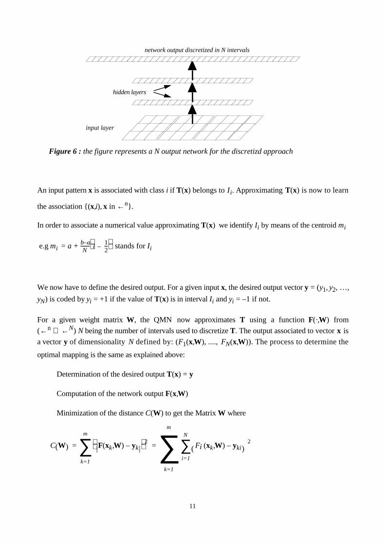
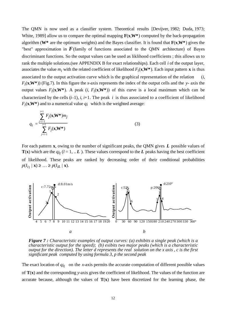
associated to the output activation curve which is the graphical representation of the relation (i,Fi(x,W*)) (Fig.7). In this figure the x-axis represents the index of the output cells and the y- axis the

output values Fi(x,W*). A peak (i, Fi(x,W*)) of this curve is a local maximum which can be

characterized by the cells (i–1), i, i+1. The peak i is thus associated to a coefficient of likelihoodFi(x,W*) and to a numerical value qi which is the weighted average:

qi =

∑j=i–1

i+1

Fj(x,W*)mj

∑j=i–1

i+1

Fj(x,W*) (3)

For each pattern x, owing to the number of significant peaks, the QMN gives L possible values ofT(x) which are the qil (l = 1, .. L ). These values correspond to the L peaks having the best coefficient

of likelihood. These peaks are ranked by decreasing order of their conditional probabilitiesp(Ii1 | x) ≥ … ≥ p(IiL | x).

Ou

tpu

t ac

tiva

tion

30 60 90 120 150180 210 240 270 300 330 360°0

c:52°d:210°

p:206°12 3

456

c:7.72m/sd:8.01m/s

12

4 5 6 7 8 9 10 11 12 13 14 15 16 17 18 1920

3

Ou

tpu

t ac

tiva

tion

a b

Figure 7 : Characteristic examples of output curves: (a) exhibits a single peak (which is acharacteristic output for the speed); (b) exibits two major peaks (which is a characteristicoutput for the direction). The letter d represents the real solution on the x axis , c is the firstsignificant peak computed by using formula 3, p the second peak

The exact location of qil on the x-axis permits the accurate computation of different possible values

of T(x) and the corresponding y-axis gives the coefficient of likelihood. The values of the function are

accurate because, although the values of T(x) have been discretized for the learning phase, the

13

interpolation of the peaks curve allows T(x) to be continuous. Looking at the different curves

obtained for each pattern of the learning set enables us to understand the “complexity” of the

function studied. Figure 7 gives two characteristic examples of the output curves obtained with the

approximation of the two transfer functions we deal with (determination of the wind speed (v) and of

the wind direction (χ)) for a given input x. The "complexity" of the phenomenon is related to the

number of significant peaks. It clearly appears that the wind speed transfer function (Fig. 7a) is

singlevalued and the related output curves exhibit a single peak. On the contrary the wind direction

transfer function is multivalued (Fig. 7b), several peaks are present showing the existence of major

ambiguities (two peaks or more).

In the following, the approach described here in which the output variable range is descretized, is

called classifier mode, in opposition to the real mode in which the output variable is estimated directly

without descretization.

3.5. NUMERICAL RESULTS

We now present results obtained using simulated scatterometer data. These results demonstrate the

validity of the NN approach and its potential to give new insight into the geophysical function.

First it is noted that the geophysical function strongly depends on the incidence angle. In fact, the

points located on the same parallel to the satellite trajectory are associated with a specific model

(Fig. 3a); different parallels (hereafter called trajectories) lead to similar models which differ only in

the values of the parameters (b1, b2, A, γ). Without any loss of generality we chose to study the

central trajectory e.g. (θ1,θ2,θ3) = (41.9°, 31.8°, 41.9°) and the two associated transfer functions T1

and T2 . The transfer functions T1 : ( )σ1, σ2, σ3 ∅ (v) and T2 : ( )σ1, σ2, σ3 ∅ (χ) are

approximated using both real and classifier QMN. Experiments were also made for others trajectories

and similar results were found.

In the classifier mode as explained above the ranges of T1 and T2 have been discretized in the

following manner : each interval Ii represents 1 m/s for the wind speed and 10°.for the wind direction

For each experiment, statistically representative learning sets have been selected, which means that the

QMN is trained with exactly the same number of patterns for each interval (this number will be

indicated for each experiment later). Each example was randomly selected from the 22 maps used for

the training (see § 2.2).

Determination of the wind speed

In the following we show how NN can be used to compute complex transfer functions and to extract

information from unknown phenomena. Real and classifier QMN are used and then compared.

14

Geophysical measurements have shown that T1 is highly non-linear. This fact has been found from

the results of preliminary experiments. The non linearity of T1 becomes important at the threshold

value of 12 m/s. Therefore this information has been taken into account by splitting the interval into

two sub intervals, each one being associated to a specific NN. Two sets of experiments were thenperformed to model the non-linearity of T1 . The performances reached were compared. Moreover, for

each experiment, dedicated neural networks were trained with both real and classifier QMN:

• the first approach consists in approximating the function on its total range [4m/s, 20m/s] by a

single QMN.

• the second approach takes the nonlinearity into account ; the function T1 is then approximated

with two different QMN. One is dedicated to low winds ranging from 4 m/s to 12 m/s, the other to

high winds from 12 m/s to 20 m/s.

In order to take these differences into account and to make the performances of the two experiments

comparable, the performances of the second experiment are given for each range separately and on the

whole range (4 m/s-20 m/s). The performances are weighted by the frequency (number of data of a

learning set over the total number of data) of each learning set (slow or high wind speed).

The architectures of the QMN used to run the experiments are now presented.

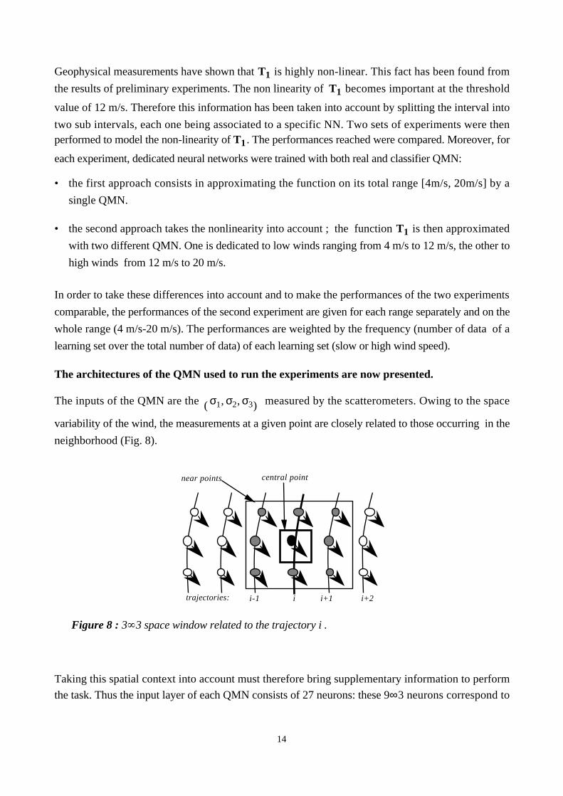
The inputs of the QMN are the ( )σ1, σ2, σ3 measured by the scatterometers. Owing to the space

variability of the wind, the measurements at a given point are closely related to those occurring in the

neighborhood (Fig. 8).

central pointnear points

trajectories: i i+1 i+2i-1

Figure 8 : 3 3 space window related to the trajectory i .

Taking this spatial context into account must therefore bring supplementary information to perform

the task. Thus the input layer of each QMN consists of 27 neurons: these 9∞3 neurons correspond to

15

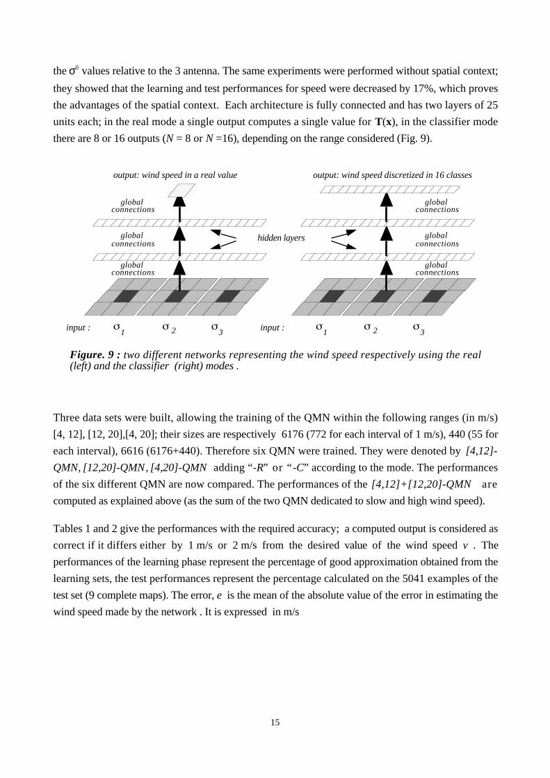
the σ0 values relative to the 3 antenna. The same experiments were performed without spatial context;

they showed that the learning and test performances for speed were decreased by 17%, which proves

the advantages of the spatial context. Each architecture is fully connected and has two layers of 25

units each; in the real mode a single output computes a single value for T(x), in the classifier mode

there are 8 or 16 outputs (N = 8 or N =16), depending on the range considered (Fig. 9).

1 2 3

output: wind speed discretized in 16 classes

hidden layers

input :

global connections

global connections

global connections

1 2 3

global

output: wind speed in a real value

input :

global connections

connections

global connections

Figure. 9 : two different networks representing the wind speed respectively using the real(left) and the classifier (right) modes .

Three data sets were built, allowing the training of the QMN within the following ranges (in m/s)

[4, 12], [12, 20],[4, 20]; their sizes are respectively 6176 (772 for each interval of 1 m/s), 440 (55 for

each interval), 6616 (6176+440). Therefore six QMN were trained. They were denoted by [4,12]-

QMN, [12,20]-QMN , [4,20]-QMN adding “-R” or “-C” according to the mode. The performances

of the six different QMN are now compared. The performances of the [4,12]+[12,20]-QMN are

computed as explained above (as the sum of the two QMN dedicated to slow and high wind speed).

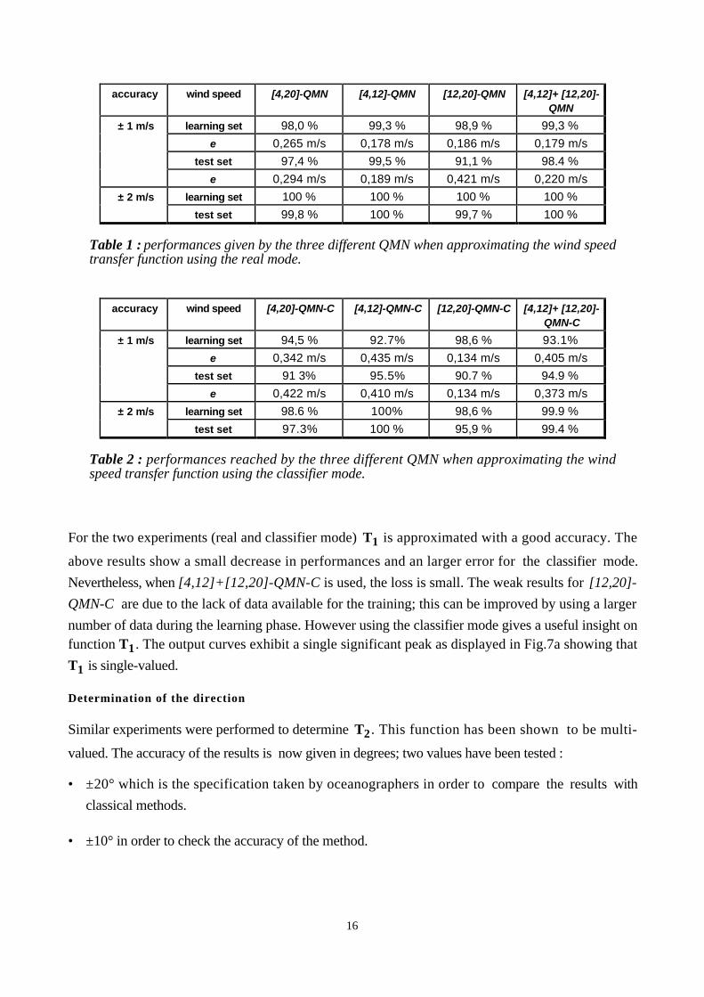
Tables 1 and 2 give the performances with the required accuracy; a computed output is considered as

correct if it differs either by 1 m/s or 2 m/s from the desired value of the wind speed v . The

performances of the learning phase represent the percentage of good approximation obtained from the

learning sets, the test performances represent the percentage calculated on the 5041 examples of the

test set (9 complete maps). The error, e is the mean of the absolute value of the error in estimating the

wind speed made by the network . It is expressed in m/s

16

accuracy wind speed [4,20]-QMN [4,12]-QMN [12,20]-QMN [4,12]+ [12,20]-

QMN

± 1 m/s learning set 98,0 % 99,3 % 98,9 % 99,3 %

e 0,265 m/s 0,178 m/s 0,186 m/s 0,179 m/s

test set 97,4 % 99,5 % 91,1 % 98.4 %

e 0,294 m/s 0,189 m/s 0,421 m/s 0,220 m/s

± 2 m/s learning set 100 % 100 % 100 % 100 %

test set 99,8 % 100 % 99,7 % 100 %

Table 1 : performances given by the three different QMN when approximating the wind speedtransfer function using the real mode.

accuracy wind speed [4,20]-QMN-C [4,12]-QMN-C [12,20]-QMN-C [4,12]+ [12,20]-

QMN-C

± 1 m/s learning set 94,5 % 92.7% 98,6 % 93.1%

e 0,342 m/s 0,435 m/s 0,134 m/s 0,405 m/s

test set 91 3% 95.5% 90.7 % 94.9 %

e 0,422 m/s 0,410 m/s 0,134 m/s 0,373 m/s

± 2 m/s learning set 98.6 % 100% 98,6 % 99.9 %

test set 97.3% 100 % 95,9 % 99.4 %

Table 2 : performances reached by the three different QMN when approximating the windspeed transfer function using the classifier mode.

For the two experiments (real and classifier mode) T1 is approximated with a good accuracy. The

above results show a small decrease in performances and an larger error for the classifier mode.

Nevertheless, when [4,12]+[12,20]-QMN-C is used, the loss is small. The weak results for [12,20]-

QMN-C are due to the lack of data available for the training; this can be improved by using a larger

number of data during the learning phase. However using the classifier mode gives a useful insight onfunction T1 . The output curves exhibit a single significant peak as displayed in Fig.7a showing that

T1 is single-valued.

Determination of the direction

Similar experiments were performed to determine T2 . This function has been shown to be multi-

valued. The accuracy of the results is now given in degrees; two values have been tested :

• ±20° which is the specification taken by oceanographers in order to compare the results with

classical methods.

• ±10° in order to check the accuracy of the method.

17

At a given wind speed the wind direction is given by a Lissajous curve; this Lissajous curve is strongly

dependent on the wind speed (Fig. 3). In order to be correctly positioned along the directrix of the

curve presented in Fig. 3, the wind speed computed above is added onto the input layer as a

supplementary information. This new information improves the accuracy of the solution. Thus the

input layer of each QMN is now composed of 30 neurons: the first 9∞3 correspond to the σo values

for each antenna using the spatial window defined above, the last three correspond to the wind speed

computed for the current trajectory in order to be correctly positioned along the directrix of the curve

presented in Fig.3. The ratio of the weight given to the wind speed (3) versus the 9∞3 σo values was

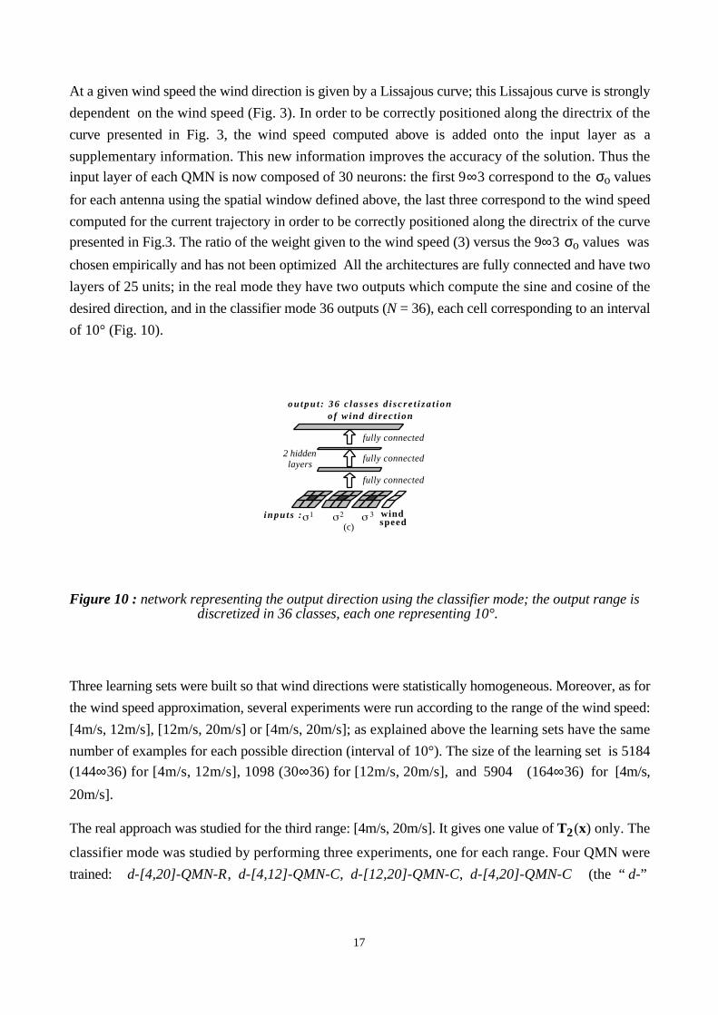
chosen empirically and has not been optimized All the architectures are fully connected and have two

layers of 25 units; in the real mode they have two outputs which compute the sine and cosine of the

desired direction, and in the classifier mode 36 outputs (N = 36), each cell corresponding to an interval

of 10° (Fig. 10).

(c)

o u t p u t : 3 6 c l a s s e s d i s c r e t i z a t i o nof w ind d i rec t ion

2 hiddenlayers

windinputs :

fully connected

fully connected

fully connected

speed

Figure 10 : network representing the output direction using the classifier mode; the output range is discretized in 36 classes, each one representing 10°.

Three learning sets were built so that wind directions were statistically homogeneous. Moreover, as for

the wind speed approximation, several experiments were run according to the range of the wind speed:

[4m/s, 12m/s], [12m/s, 20m/s] or [4m/s, 20m/s]; as explained above the learning sets have the same

number of examples for each possible direction (interval of 10°). The size of the learning set is 5184

(144∞36) for [4m/s, 12m/s], 1098 (30∞36) for [12m/s, 20m/s], and 5904 (164∞36) for [4m/s,

20m/s].

The real approach was studied for the third range: [4m/s, 20m/s]. It gives one value of T2(x) only. The

classifier mode was studied by performing three experiments, one for each range. Four QMN were

trained: d-[4,20]-QMN-R, d-[4,12]-QMN-C, d-[12,20]-QMN-C, d-[4,20]-QMN-C (the “ d-”

18

indicates that the direction is concerned). Performances were also computed on d-[4,12]+[12,20]-

QMN-C.

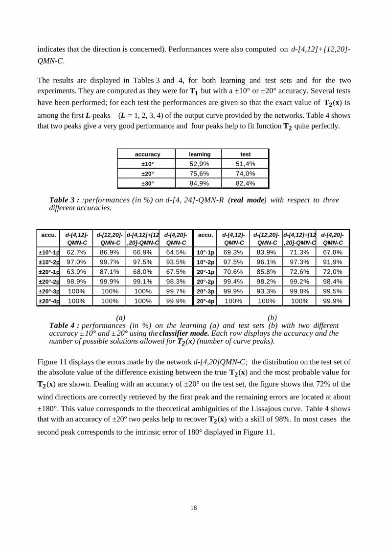
The results are displayed in Tables 3 and 4, for both learning and test sets and for the twoexperiments. They are computed as they were for T1 but with a ±10° or ±20° accuracy. Several tests

have been performed; for each test the performances are given so that the exact value of T2(x) is

among the first L-peaks (L = 1, 2, 3, 4) of the output curve provided by the networks. Table 4 showsthat two peaks give a very good performance and four peaks help to fit function T2 quite perfectly.

accuracy learning test

±10° 52,9% 51,4%

±20° 75,6% 74,0%

±30° 84,9% 82,4%

Table 3 : :performances (in %) on d-[4, 24]-QMN-R (real mode) with respect to threedifferent accuracies.

accu. d-[4,12]-

QMN-C

d-[12,20]-

QMN-C

d-[4,12]+[12

,20]-QMN-C

d-[4,20]-

QMN-C

accu. d-[4,12]-

QMN-C

d-[12,20]-

QMN-C

d-[4,12]+[12

,20]-QMN-C

d-[4,20]-

QMN-C

±10°-1p 62.7% 86.9% 66.9% 64.5% 10°-1p 69.3% 83.9% 71.3% 67.8%

±10°-2p 97.0% 99.7% 97.5% 93.5% 10°-2p 97.5% 96.1% 97.3% 91,9%

±20°-1p 63.9% 87.1% 68.0% 67.5% 20°-1p 70.6% 85.8% 72.6% 72,0%

±20°-2p 98.9% 99.9% 99.1% 98.3% 20°-2p 99.4% 98.2% 99.2% 98.4%

±20°-3p 100% 100% 100% 99.7% 20°-3p 99.9% 93.3% 99.8% 99.5%

±20°-4p 100% 100% 100% 99.9% 20°-4p 100% 100% 100% 99.9%

(a) (b)Table 4 : performances (in %) on the learning (a) and test sets (b) with two differentaccuracy ±10° and ±20° using the classifier mode. Each row displays the accuracy and thenumber of possible solutions allowed for T2(x) (number of curve peaks).

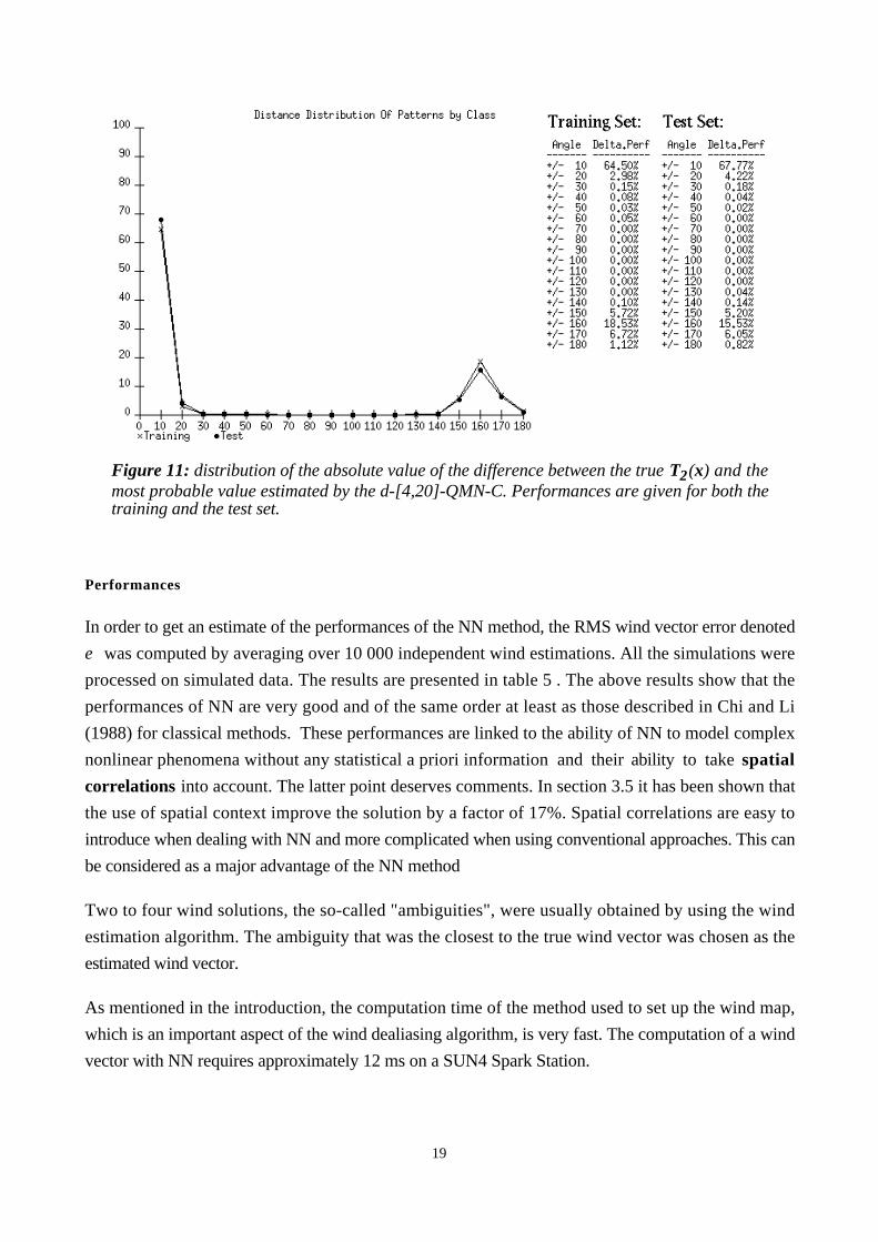
Figure 11 displays the errors made by the network d-[4,20]QMN-C ; the distribution on the test set ofthe absolute value of the difference existing between the true T2(x) and the most probable value for

T2(x) are shown. Dealing with an accuracy of ±20° on the test set, the figure shows that 72% of the

wind directions are correctly retrieved by the first peak and the remaining errors are located at about

±180°. This value corresponds to the theoretical ambiguities of the Lissajous curve. Table 4 showsthat with an accuracy of ±20° two peaks help to recover T2(x) with a skill of 98%. In most cases the

second peak corresponds to the intrinsic error of 180° displayed in Figure 11.

19

Figure 11: distribution of the absolute value of the difference between the true T2(x) and themost probable value estimated by the d-[4,20]-QMN-C. Performances are given for both thetraining and the test set.

Performances

In order to get an estimate of the performances of the NN method, the RMS wind vector error denoted

e was computed by averaging over 10 000 independent wind estimations. All the simulations were

processed on simulated data. The results are presented in table 5 . The above results show that the

performances of NN are very good and of the same order at least as those described in Chi and Li

(1988) for classical methods. These performances are linked to the ability of NN to model complex

nonlinear phenomena without any statistical a priori information and their ability to take spatial

correlations into account. The latter point deserves comments. In section 3.5 it has been shown that

the use of spatial context improve the solution by a factor of 17%. Spatial correlations are easy to

introduce when dealing with NN and more complicated when using conventional approaches. This can

be considered as a major advantage of the NN method

Two to four wind solutions, the so-called "ambiguities", were usually obtained by using the wind

estimation algorithm. The ambiguity that was the closest to the true wind vector was chosen as the

estimated wind vector.

As mentioned in the introduction, the computation time of the method used to set up the wind map,

which is an important aspect of the wind dealiasing algorithm, is very fast. The computation of a wind

vector with NN requires approximately 12 ms on a SUN4 Spark Station.

20

Speed d-[4,20]-QMN-C

low 0.32

Middle 0.40

Hight 1.18

Table 5 : e (in m/s) for tthe [4,20]-QMN-C.

The different QMN are now chained together in order to solve the complete problem which is the

drawing up of a correct wind map. Section 4 presents the “Neural Machine”. Section 4.1 is devoted

to the presentation of the complete architecture. The results listed in section 4.2 deal with the same

data as before.

4. THE “NEURAL MACHINE” (NM)

As we have seen, the wind speed and the wind direction are computed by two different modules

composed of two and one QMN respectively. In fact the two modules are not independent. A Neural

Machine [Thiria et al., 1992] has accordingly been designed in order to connect them and to compute

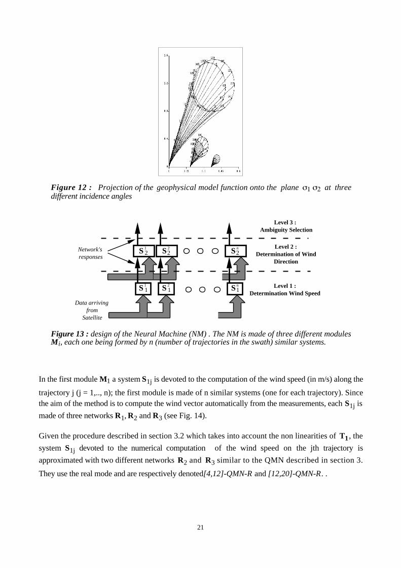
the wind vector automatically. The NM is formed by the association of three different modules. The

first module M1 determines the wind speed at each point of the swath. The results are then supplied

to the second module M2 as a supplementary data to compute the wind direction. A third module M3

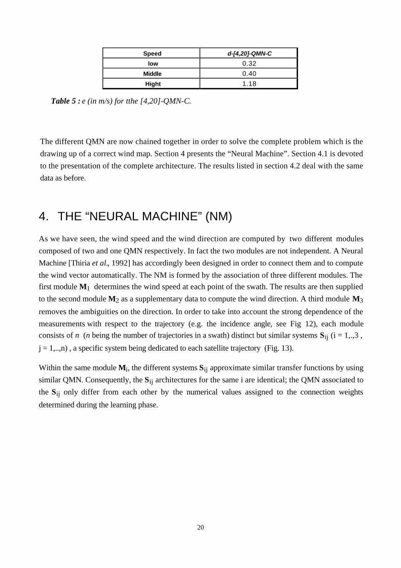
removes the ambiguities on the direction. In order to take into account the strong dependence of the

measurements with respect to the trajectory (e.g. the incidence angle, see Fig 12), each module

consists of n (n being the number of trajectories in a swath) distinct but similar systems Sij (i = 1,.,3 ,

j = 1,..,n) , a specific system being dedicated to each satellite trajectory (Fig. 13).

Within the same module Mi, the different systems Sij approximate similar transfer functions by using

similar QMN. Consequently, the Sij architectures for the same i are identical; the QMN associated to

the Sij only differ from each other by the numerical values assigned to the connection weights

determined during the learning phase.

21

Figure 12 : Projection of the geophysical model function onto the plane at threedifferent incidence angles

Level 3 : Ambiguity Selection

Level 2 :Determination of Wind

Direction

Level 1 :Determination Wind Speed

Data arriving from

Satellite

Network's responses

11S

21S

12S

22S 2

nS

1nS

Figure 13 : design of the Neural Machine (NM) . The NM is made of three different modulesMi, each one being formed by n (number of trajectories in the swath) similar systems.

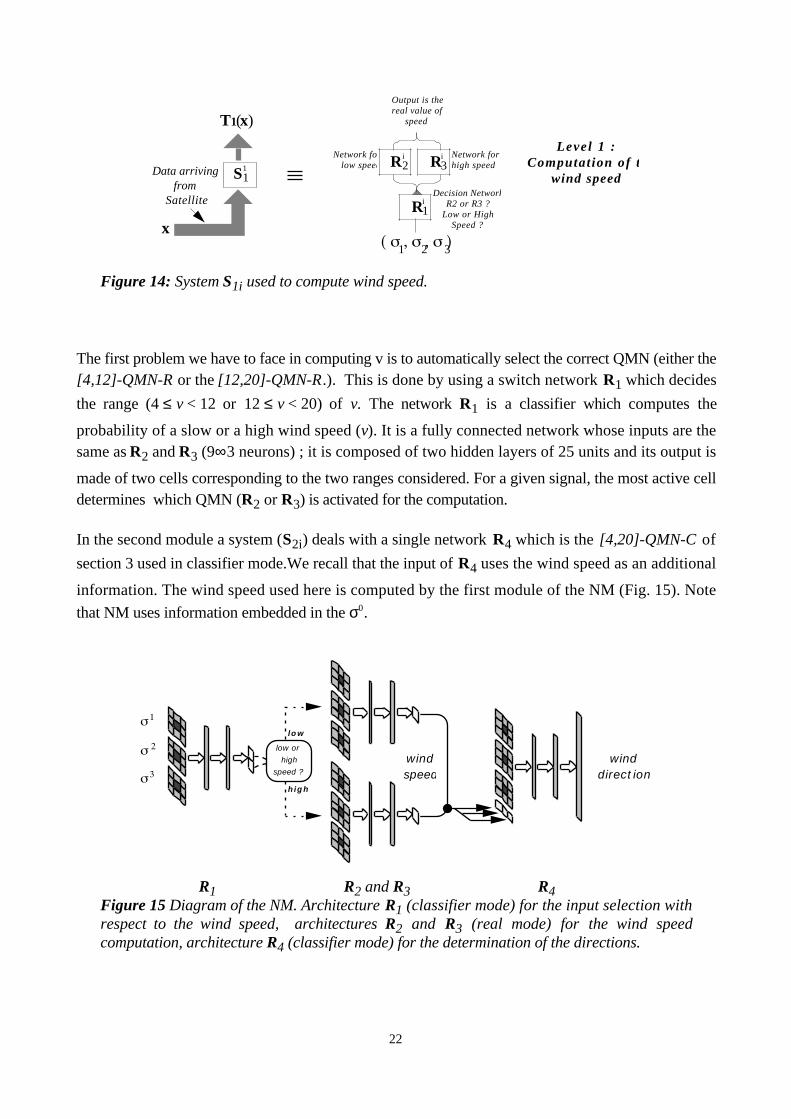
In the first module M1 a system S1j is devoted to the computation of the wind speed (in m/s) along the

trajectory j (j = 1,.., n); the first module is made of n similar systems (one for each trajectory). Sincethe aim of the method is to compute the wind vector automatically from the measurements, each S1j is

made of three networks R1, R2 and R3 (see Fig. 14).

Given the procedure described in section 3.2 which takes into account the non linearities of T1 , the

system S1j devoted to the numerical computation of the wind speed on the jth trajectory is

approximated with two different networks R2 and R3 similar to the QMN described in section 3.

They use the real mode and are respectively denoted[4,12]-QMN-R and [12,20]-QMN-R. .

22

Level 1 :Computat ion of the

wind speedData arriving

fromSatellite

11S

R1i

R3iR2

i

Decision Network R2 or R3 ?

Low or High Speed ?

Network for high speed

Network for low speed

Output is the real value of

speed

x

T1(x)

1 2 3

Figure 14: System S1i used to compute wind speed.

The first problem we have to face in computing v is to automatically select the correct QMN (either the[4,12]-QMN-R or the [12,20]-QMN-R.). This is done by using a switch network R1 which decides

the range (4 ≤ v < 12 or 12 ≤ v < 20) of v. The network R1 is a classifier which computes the

probability of a slow or a high wind speed (v). It is a fully connected network whose inputs are thesame as R2 and R3 (9∞3 neurons) ; it is composed of two hidden layers of 25 units and its output is

made of two cells corresponding to the two ranges considered. For a given signal, the most active celldetermines which QMN (R2 or R3) is activated for the computation.

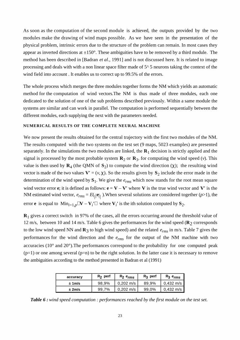
In the second module a system (S2i) deals with a single network R4 which is the [4,20]-QMN-C of

section 3 used in classifier mode.We recall that the input of R4 uses the wind speed as an additional

information. The wind speed used here is computed by the first module of the NM (Fig. 15). Note

that NM uses information embedded in the σ0.

low or

high

speed ?

low

high

wind speed

wind direction

R1 R2 and R3 R4Figure 15 Diagram of the NM. Architecture R1 (classifier mode) for the input selection withrespect to the wind speed, architectures R2 and R3 (real mode) for the wind speedcomputation, architecture R4 (classifier mode) for the determination of the directions.

23

As soon as the computation of the second module is achieved, the outputs provided by the two

modules make the drawing of wind maps possible. As we have seen in the presentation of the

physical problem, intrinsic errors due to the structure of the problem can remain. In most cases they

appear as inverted directions at ±150°. These ambiguities have to be removed by a third module. The

method has been described in [Badran et al., 1991] and is not discussed here. It is related to image

processing and deals with with a non linear space filter made of 5^5 neurons taking the context of the

wind field into account . It enables us to correct up to 99.5% of the errors.

The whole process which merges the three modules together forms the NM which yields an automatic

method for the computation of wind vectors.The NM is thus made of three modules, each one

dedicated to the solution of one of the sub problems described previously. Within a same module the

systems are similar and can work in parallel. The computation is performed sequentially between the

different modules, each supplying the next with the parameters needed.

NUMERICAL RESULTS OF THE COMPLETE NEURAL MACHINE

We now present the results obtained for the central trajectory with the first two modules of the NM.

The results computed with the two systems on the test set (9 maps, 5023 examples) are presentedseparately. In the simulations the two modules are linked, the R1 decision is strictly applied and the

signal is processed by the most probable system R2 or R3. for computing the wind speed (v). This

value is then used by R4 (the QMN of S2) to compute the wind direction (χ); the resulting wind

vector is made of the two values V' = (v, χ). So the results given by S2 include the error made in the

determination of the wind speed by S1. We give the erms which now stands for the root mean square

wind vector error e; it is defined as follows: e = V – V' where V is the true wind vector and V' is theNM estimated wind vector, erms = E(| || |e ).When several solutions are considered together (p>1), the

error e is equal to Mini=1,p∧V – Vi'∧ where Vi' is the ith solution computed by S2.

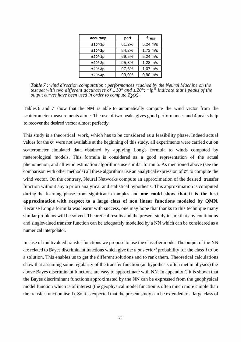
R1 gives a correct switch in 97% of the cases, all the errors occurring around the threshold value of

12 m/s, between 10 and 14 m/s. Table 6 gives the performances for the wind speed (R2 corresponds

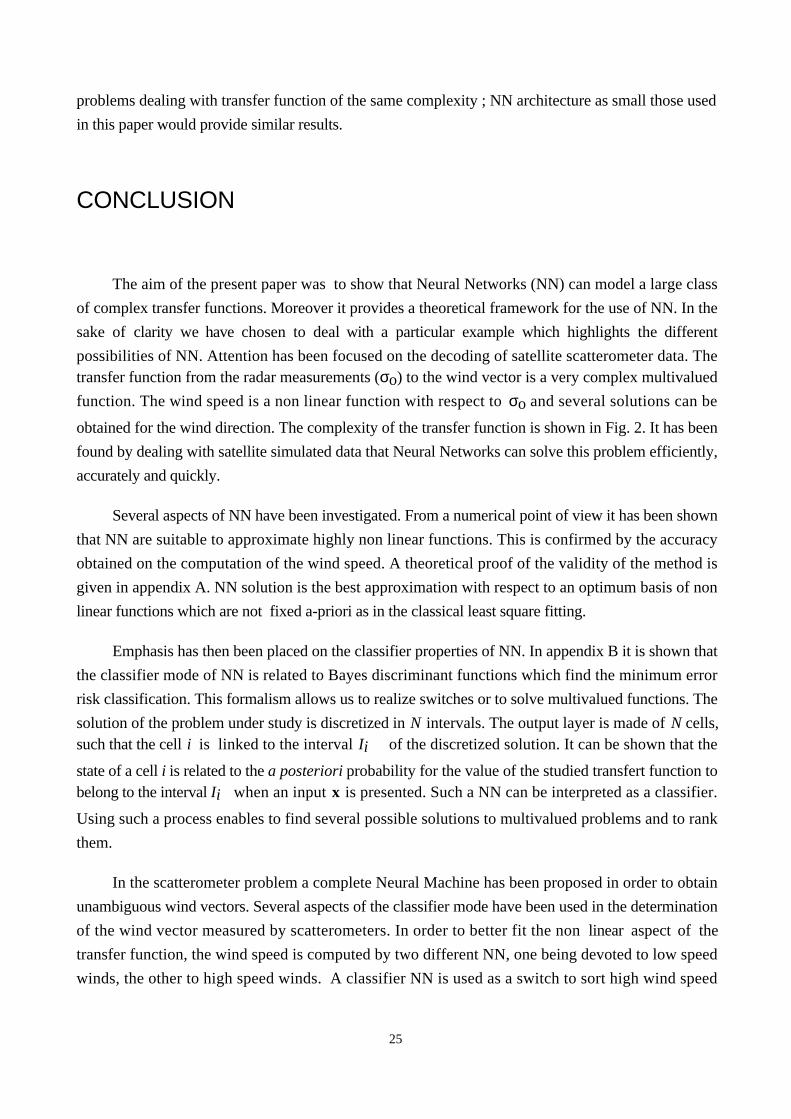
to the low wind speed NN and R3 to high wind speed) and the related erms in m/s. Table 7 gives the

performances for the wind direction and the erms for the output of the NM machine with two

accuracies (10° and 20°).The performances correspond to the probability for one computed peak

(p=1) or one among several (p=n) to be the right solution. In the latter case it is necessary to remove

the ambiguities according to the method presented in Badran et al (1991)

accuracy R2 perf R2 erms R3 perf R3 erms

± 1m/s 98,9% 0,202 m/s 89,9% 0,432 m/s

± 2m/s 99,7% 0,202 m/s 99,0% 0,432 m/s

Table 6 : wind speed computation : performances reached by the first module on the test set.

24

accuracy perf erms

±10°-1p 61,2% 5,24 m/s

±10°-2p 84,2% 1,73 m/s

±20°-1p 69,5% 5,24 m/s

±20°-2p 95,8% 1,28 m/s

±20°-3p 97,6% 1,07 m/s

±20°-4p 99,0% 0,90 m/s

Table 7 : wind direction computation : performances reached by the Neural Machine on thetest set with two different accuracies of ±10° and ±20°; “ip” indicate that i peaks of theoutput curves have been used in order to compute T2(x).

Tables 6 and 7 show that the NM is able to automatically compute the wind vector from the

scatterometer measurements alone. The use of two peaks gives good performances and 4 peaks help

to recover the desired vector almost perfectly.

This study is a theoretical work, which has to be considered as a feasibility phase. Indeed actual

values for the σ0 were not available at the beginning of this study, all experiments were carried out on

scatterometer simulated data obtained by applying Long's formula to winds computed by

meteorological models. This formula is considered as a good representation of the actual

phenomenon, and all wind estimation algorithms use similar formula. As mentioned above (see the

comparison with other methods) all these algorithms use an analytical expression of σ0 to compute the

wind vector. On the contrary, Neural Networks compute an approximation of the desired transfer

function without any a priori analytical and statistical hypothesis. This approximation is computed

during the learning phase from significant examples and one could show that it is the best

approximation with respect to a large class of non linear functions modeled by QMN.

Because Long's formula was learnt with success, one may hope that thanks to this technique many

similar problems will be solved. Theoretical results and the present study insure that any continuous

and singlevalued transfer function can be adequately modelled by a NN which can be considered as a

numerical interpolator.

In case of multivalued transfer functions we propose to use the classifier mode. The output of the NN

are related to Bayes discriminant functions which give the a posteriori probability for the class i to be

a solution. This enables us to get the different solutions and to rank them. Theoretical calculations

show that assuming some regularity of the transfer function (an hypothesis often met in physics) the

above Bayes discriminant functions are easy to approximate with NN. In appendix C it is shown that

the Bayes discriminant functions approximated by the NN can be expressed from the geophysical

model function which is of interest (the geophysical model function is often much more simple than

the transfer function itself). So it is expected that the present study can be extended to a large class of

25

problems dealing with transfer function of the same complexity ; NN architecture as small those used

in this paper would provide similar results.

CONCLUSION

The aim of the present paper was to show that Neural Networks (NN) can model a large class

of complex transfer functions. Moreover it provides a theoretical framework for the use of NN. In the

sake of clarity we have chosen to deal with a particular example which highlights the different

possibilities of NN. Attention has been focused on the decoding of satellite scatterometer data. Thetransfer function from the radar measurements (σo) to the wind vector is a very complex multivalued

function. The wind speed is a non linear function with respect to σo and several solutions can be

obtained for the wind direction. The complexity of the transfer function is shown in Fig. 2. It has been

found by dealing with satellite simulated data that Neural Networks can solve this problem efficiently,

accurately and quickly.

Several aspects of NN have been investigated. From a numerical point of view it has been shown

that NN are suitable to approximate highly non linear functions. This is confirmed by the accuracy

obtained on the computation of the wind speed. A theoretical proof of the validity of the method is

given in appendix A. NN solution is the best approximation with respect to an optimum basis of non

linear functions which are not fixed a-priori as in the classical least square fitting.

Emphasis has then been placed on the classifier properties of NN. In appendix B it is shown that

the classifier mode of NN is related to Bayes discriminant functions which find the minimum error

risk classification. This formalism allows us to realize switches or to solve multivalued functions. The

solution of the problem under study is discretized in N intervals. The output layer is made of N cells,such that the cell i is linked to the interval Ii of the discretized solution. It can be shown that the

state of a cell i is related to the a posteriori probability for the value of the studied transfert function tobelong to the interval Ii when an input x is presented. Such a NN can be interpreted as a classifier.

Using such a process enables to find several possible solutions to multivalued problems and to rank

them.

In the scatterometer problem a complete Neural Machine has been proposed in order to obtain

unambiguous wind vectors. Several aspects of the classifier mode have been used in the determination

of the wind vector measured by scatterometers. In order to better fit the non linear aspect of the

transfer function, the wind speed is computed by two different NN, one being devoted to low speed

winds, the other to high speed winds. A classifier NN is used as a switch to sort high wind speed

26

versus low wind speed and turn the input towards the dedicated NN. This switch improves the

accuracy of the computation by allowing the computations to be done by an adequate NN. The wind

direction is also determined by a NN used in classifier mode. In many cases several directions

corresponding to several significant coefficients of likelihood are found. The remaining ambiguities

are then removed by assuming that there is some space coherence of the wind vector [Badran et al,

1991] .

In section 3 several methods to retrieve the scatterometer wind have been compared. It appears

that the NN have the best performance. From the above complex example we can claim that NN

constitute a powerful tool to model a large class of transfer functions. In fact the NN are able to solve

many problems encountered in physics. A major advantage of NN is their ability to extract

information in a noisy environnement whatever the noise.

It has been found that NN are suitable to model non linear filters. Filtering is a technique often

used in geophysics to remove noise or to take advantages of the information embedded in time

intervals or space contexts. Such a filter has been used with success to remove the scatterometer wind

ambiguities by Schlutz (1990). NN provides the optimum filter with respect to the studied problem

(Badran et al , 1991).

NN are also suitable to solve complex inverse problems. The direct problem provides a suitable

basis of examples which can be learned the other way around , the output of the direct problem being

considered as the input of the inverse problem. The NN then computes a statistical model of the

inverse problem. In fact the simulated scatterometer example presented in this paper can be considered

as an inversion of Long's formula.

NN present many other advantages. It is very easy to take into account new parameters even if

their dependence cannot be established in the form of an equation. New cells related to these new

parameters are added to the input layer and connected to the hidden layers. In the scatterometer case it

would be easy to investigate how sensitive the solution is to the introduction of additional variables

such as wind waves which are supposed to influence the transfer function at low wind speed.

The methodology developed in the present study will be applied to ERS1 scatterometer data as

soon as they are available. The determination and calibration of a Geophysical Model can be

bypassed. In fact the Geophysical Model is embedded in the architecture of the NN machine

described above. The NN machine will be calibrated during a learning phase on the output provided y

a fine grid mesh meteorological model such as the PERIDOT model of the French Met Office

(Météo-France). It is during this confrontation with the real world that the usefulness of NN should be

definitely established.

27

Acknowledgments

This work was supported by CNRS (Centre National de la Recherche Scientifique), PNTS

(Programme national de Télédétection Spatiale) and SGDN (Service General de la Défense

Nationale). The simulations were run by using the SN2 software provided by the Neuristic

Compagny. We are grateful to V. Cassé and C. Gaffard for stimulating discussions. We thank P.

Braconnot and M. Boukthir for providing the data set. Useful comments were provided by an

anonymous referee.

28

APPENDICES

APPENDIX A

QMN AND FUNCTION APPROXIMATION

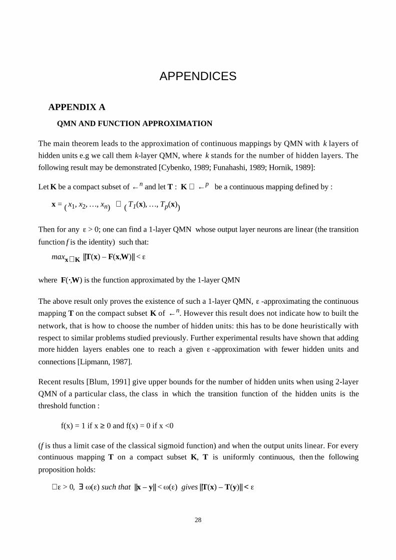
The main theorem leads to the approximation of continuous mappings by QMN with k layers of

hidden units e.g we call them k-layer QMN, where k stands for the number of hidden layers. The

following result may be demonstrated [Cybenko, 1989; Funahashi, 1989; Hornik, 1989]:

Let K be a compact subset of ←n and let T : K ∅ ←p be a continuous mapping defined by :

x = ( )x1, x2, …, xn ∅ ( )T1(x), …, Tp(x)

Then for any > 0; one can find a 1-layer QMN whose output layer neurons are linear (the transition

function f is the identity) such that:

maxx∈K ||T(x) – F(x,W)|| <

where F(·,W) is the function approximated by the 1-layer QMN

The above result only proves the existence of such a 1-layer QMN, -approximating the continuous

mapping T on the compact subset K of ←n. However this result does not indicate how to built the

network, that is how to choose the number of hidden units: this has to be done heuristically with

respect to similar problems studied previously. Further experimental results have shown that adding

more hidden layers enables one to reach a given -approximation with fewer hidden units and

connections [Lipmann, 1987].

Recent results [Blum, 1991] give upper bounds for the number of hidden units when using 2-layer

QMN of a particular class, the class in which the transition function of the hidden units is the

threshold function :

f(x) = 1 if x ≥ 0 and f(x) = 0 if x <0

(f is thus a limit case of the classical sigmoid function) and when the output units linear. For every

continuous mapping T on a compact subset K, T is uniformly continuous, then the following

proposition holds:

∀ > 0, ( ) such that ||x – y|| < ( ) gives ||T(x) – T(y)|| <

29

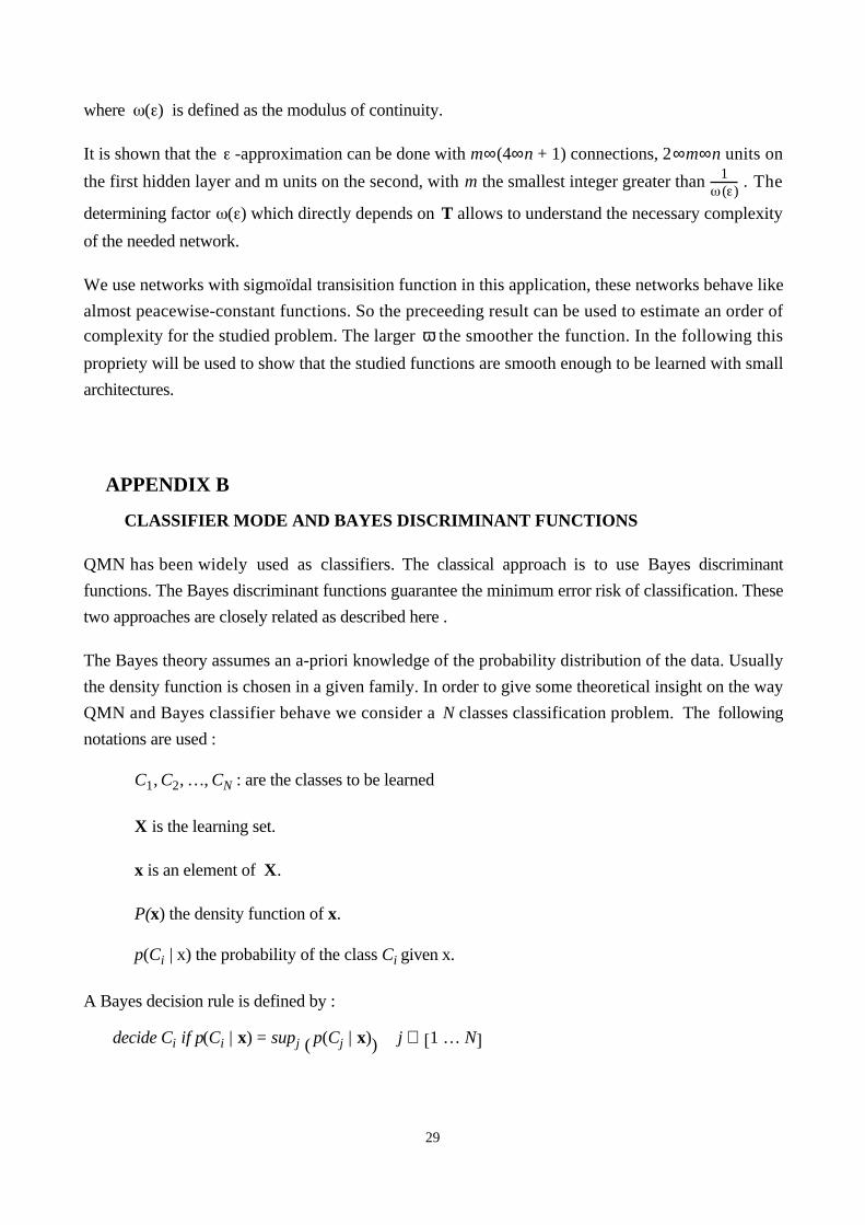
where ( ) is defined as the modulus of continuity.

It is shown that the -approximation can be done with m∞(4∞n + 1) connections, 2∞m∞n units on

the first hidden layer and m units on the second, with m the smallest integer greater than 1( )

. The

determining factor ( ) which directly depends on T allows to understand the necessary complexity

of the needed network.

We use networks with sigmoïdal transisition function in this application, these networks behave like

almost peacewise-constant functions. So the preceeding result can be used to estimate an order of

complexity for the studied problem. The larger ω the smoother the function. In the following this

propriety will be used to show that the studied functions are smooth enough to be learned with small

architectures.

APPENDIX B

CLASSIFIER MODE AND BAYES DISCRIMINANT FUNCTIONS

QMN has been widely used as classifiers. The classical approach is to use Bayes discriminant

functions. The Bayes discriminant functions guarantee the minimum error risk of classification. These

two approaches are closely related as described here .

The Bayes theory assumes an a-priori knowledge of the probability distribution of the data. Usually

the density function is chosen in a given family. In order to give some theoretical insight on the way

QMN and Bayes classifier behave we consider a N classes classification problem. The following

notations are used :

C1, C2, …, CN : are the classes to be learned

X is the learning set.

x is an element of X.

P(x) the density function of x.

p(Ci | x) the probability of the class Ci given x.

A Bayes decision rule is defined by :

decide Ci if p(Ci | x) = supj ( )p(Cj | x) j ∈ [ ]1 … N

30

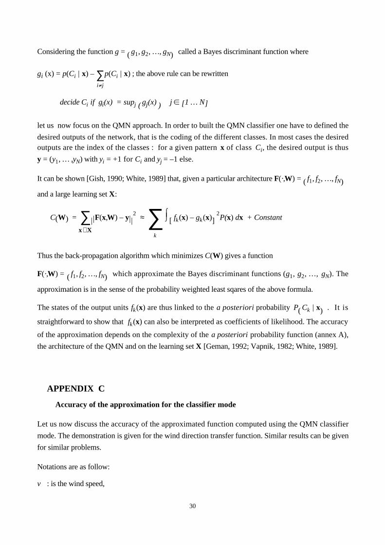
Considering the function g = ( )g1, g2, …, gN called a Bayes discriminant function where

gi (x) = p(Ci | x) – ∑i j

p(Ci | x) ; the above rule can be rewritten

decide Ci if gi(x) = supj ( )gj(x) j [ ]1 … N

let us now focus on the QMN approach. In order to built the QMN classifier one have to defined the

desired outputs of the network, that is the coding of the different classes. In most cases the desiredoutputs are the index of the classes : for a given pattern x of class Ci, the desired output is thus

y = (y1, … ,yN) with yi = +1 for Ci and yj = –1 else.

It can be shown [Gish, 1990; White, 1989] that, given a particular architecture F(·,W) = ( )f1, f2, …, fN

and a large learning set X:

C( )W = ∑x∈X

| || |F(x,W) – y2 ≈ ∑

k

⌡⌠[ ]fk(x) – gk(x)2P(x) dx + Constant

Thus the back-propagation algorithm which minimizes C(W) gives a function

F(·,W) = ( )f1, f2, …, fN which approximate the Bayes discriminant functions (g1, g2, …, gN). The

approximation is in the sense of the probability weighted least sqares of the above formula.

The states of the output units fk(x) are thus linked to the a posteriori probability P( )Ck | x . It is

straightforward to show that fk(x) can also be interpreted as coefficients of likelihood. The accuracy

of the approximation depends on the complexity of the a posteriori probability function (annex A),

the architecture of the QMN and on the learning set X [Geman, 1992; Vapnik, 1982; White, 1989].

APPENDIX C

Accuracy of the approximation for the classifier mode

Let us now discuss the accuracy of the approximated function computed using the QMN classifier

mode. The demonstration is given for the wind direction transfer function. Similar results can be given

for similar problems.

Notations are as follow:

v : is the wind speed,

31

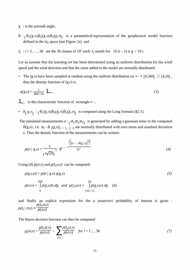
χ : is the azimuth angle,

^ : ( )σ̂1(χ,v),σ̂2(χ,v),σ̂3(χ,v) is a parametrical representation of the geophysical model function

defined in the σo space (see Figure 2a) and

Ii : i = 1, …, 36 are the 36 classes of 10° each: Ii stands for: 10 (i – 1) ≤ χ < 10 i.

Let us assume that the learning set has been determined using an uniform distribution for the wind

speed and the wind direction and that the noise added to the model are normally distributed:

• The (χ,v) have been sampled at random using the uniform distribution on = [ ]0,360 ⊗ [ ]4,20 ,

thus the density function of (χ,v) is

: q(χ,v) = 1360⊗16

1 , (3)

1 is the characteristic function of rectangle .

• ^( )χ,v : ( )σ̂1(χ,v),σ̂2(χ,v),σ̂3(χ,v) is computed using the Long formula (§2.1).

The simulated measurements : ( )σ1,σ2,σ3 is generated by adding a gaussian noise to the computed^(χ,v) , i.e. σi - σ̂ i(χ,v)|i = 1, 2, 3 are normally distributed with zero mean and standard deviation

s. Thus the density function of the measurements can be written:

p( | χ,v) = 1

( )s 2π3 . e –

| | – ^(χ,v)2

2s2 (4)

Using (4) p( ,v) and p(Ii, ,v) can be computed:

p(χ,v, ) = p(σ | χ,v) q(χ,v) (5)

p( ,v) = ⌡⌠0

360

p(χ,v,σ) dχ and p(Ii, ,v) = ⌡⌠10(i–1)

10 i

p(χ, ,v) dχ (6)

and finally an explicit expression for the a posteriori probability of interest is given :

p(Ii | σ,v) = p(Ii, ,v)p( ,v)

The Bayes decision function can then be computed:

gi( ,v) = p(Ii,σ,v)p( ,v) – ∑

j i

p(Ij, ,v)p( ,v) for i = 1 ,. , 36 (7)

32

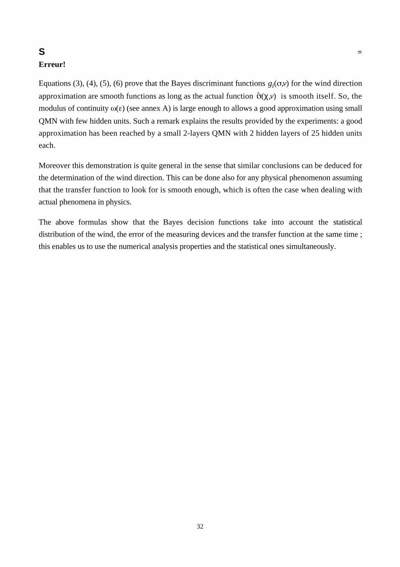
S =

Erreur!

Equations (3), (4), (5), (6) prove that the Bayes discriminant functions gi( ,v) for the wind direction

approximation are smooth functions as long as the actual function ^ (χ,v) is smooth itself. So, the

modulus of continuity ( ) (see annex A) is large enough to allows a good approximation using small

QMN with few hidden units. Such a remark explains the results provided by the experiments: a good

approximation has been reached by a small 2-layers QMN with 2 hidden layers of 25 hidden units

each.

Moreover this demonstration is quite general in the sense that similar conclusions can be deduced for

the determination of the wind direction. This can be done also for any physical phenomenon assuming

that the transfer function to look for is smooth enough, which is often the case when dealing with

actual phenomena in physics.

The above formulas show that the Bayes decision functions take into account the statistical

distribution of the wind, the error of the measuring devices and the transfer function at the same time ;

this enables us to use the numerical analysis properties and the statistical ones simultaneously.

33

REFERENCES

Badran, F., S. Thiria, and M. Crepon, Wind ambiguity removal by the use of neural network

techniques, Journal of.Geophysical.Research, 96, NO. C11, 20 521-20 529, Nov 15, 1991.

Battititi, R., First and second order Methods for learning: Between Steepest descent and Newton's

Method, Neural computation, 4, 141-166, 1992.

Blum, E., and L. Li, Approximation theory and feedforward networks, Neural Networks, 4, 511-515,

1991.

Bourlard, H., and C.J. Wellekens, Links between Markov models and multilayer perceptrons, IEEE

Transaction. Pattern Anal. Machine Intell, 12, 1167-1178, 1990.

Cavanié A. and D. Offiler : ERS1 Wind Scatterometer : Wind Extraction and Ambiguity Removal.

Proceedings of IGARS 86 Symposium, Zurich, ( ESA SP-254), 1986

Cybenko, G., Approximation by superposition of sigmoidal function, Mathematics of Control, Signal

and Systems, 2, 303-314, 1989.

Devijver P., and J Kittler, Statistical Pattern Recognition, Prentice Hall, 1982.

Duda, R. O., and P.E Hart, Pattern Classification and Scene Analysis, John Wiley, New York, 1973.

Freilich, M.H., and D. B. Chelton, Wave number spectra of Pacific winds measured by the Seasat

scatterometer, J. Phys. Oceanogr., 16, 741-757, 1986.

Funahashi, K.I., On the approximate realization of continuous mappings by neural networs, Neural

Networks, 2, 183-192, 1989.

Geman, S., E. Bienenstock, and R. Doursat, Neural Network and the Bias variance dilemna, Neural

computation, 4, 1-58, 1992.

Gish, H., A probabilistic approach of the understanding and training of neural network classifiers,

ICASSP, 3, 1361-1364, New Mexico, 1990.

Hornik, K., M. Stinchcomb, and H. White, Multi-layer feedforward networks are universal

approximators, Neural Networks, 2, 359-366, 1989.

34

Lecun, Y., Boser B, Henderson D.,Howard R.E.,Hubbard and Jackel L.D. : Handwritten digit

recognition with a back-propagation network, Neural information Processing Systems 2, 396-404,

ed by D.S. Touretzki, Morgan Kaufmann.

Lipmann, R.P., An introduction to computing with neural nets, IEEE ASSP Magazine, 4-21, 1987.

Lipmann, R.P., Rewiew of neural netwoks for speech recognition, Neural Computation, 1, 1-38, 1989.

Long A. E. Towards a C-Band Radar Sea Echo Model for the ERS1 Scatterometer. Proc. First Int.

Coll. on Spectral Signatures, ESA, Les Arcs, 1986

Price J. C. The nature of Multiple Solution of Surface Wind Speed Over the Oceans from

Scatterometer Measurement. Remote Sensing of Environement, 5, 47-74, American Elsevier

Publishing Compagny, 1976

Roquet, H. , and Ratier A., Toward direct assimilation of scatterometer backscatter measurements into

numerical weather predction models, Proceedings of the IGARSS'88 Symposium, Eur. Space

Agency Spec. Publ. ESA SP-284, 257-260, 1988

Rumelhart, D.E., J.L. MacClelland, and the PDP Research Group, Parallel Distributed Processing:

explorations in the microstructures of cognition, MIT Press, 1986

Schultz, H., A circular median filter approach for resolving directionnal ambiguities in wind fieldd

retrieved from spaceborn scatterometer data, J. Geophys. Res., 95, 5291-5304, 1990.

Thiria, S., C. Mejia, F. Badran, and M. Crepon, Multimodular Architecture for Remote Sensing

Operations, Neural Information Processing System, 4, R. Lippmann, J.E. Moody, Touretzky Ed.,

1992.

Vapnik, V., Estimation of dependences based on empirical data, Springer Verlag, New York, 1982.

White, H., Learning in Artificial Neural Networks: A Statistical Perspective, Neural Computation , 1,

425-464, 1989.

Widrow, B., S.D. Stearns, Adaptative Signal Processing, Prentice Hall, Englewood Cliffs NJ, 1985.