A model for holding strategy in public transit systems with real-time information
12
A model for holding strategy in public transit systems with real-time information Saeed Zolfaghari * , Nader Azizi, Mohamad Y. Jaber Department of Mechanical and Industrial Engineering, Ryerson University, Toronto, Ont., Canada M5B 2K3 Abstract Holding strategies are among the most commonly used operation-control strategies in public transit systems. These strategies are most effective when used to control services characterized by high frequency. In this paper, a mathematical model for a holding con- trol strategy is developed. Particularly, this model uses real-time information of locations of buses along a specified route. The objec- tive of the developed model is to minimize the waiting time of passengers at all stops on that route. Furthermore, the model developed in this paper is characterized by the flexibility of adopting situations where bus occupancy could be either high, or low. A heuristic is developed to circumvent the complexity of the solution for the problem described. Numerical examples and com- putational results are presented and discussed. Ó 2005 Elsevier Ltd. All rights reserved. Keywords: Public transit; Holding strategies; Real-time information; Simulated annealing; Heuristics; Passengers waiting time 1. Introduction In most major cities, levels of traffic congestion are rising along with their associated problems such as tra- vel delays and pollution. While any increase in public transit rider-ship could reduce the level of traffic conge- stion and related costs, most transit agencies are not able to expand their existing services because of fiscal and physical constraints. As a result, there is growing interest in the use of new technologies to maximize tran- sit system efficiency and productivity. In transit systems, public or private, providing a reli- able service is the main objective of operation managers. Dependable schedules, minimum passengers waiting time, and short travel times are some instances of reli- able services. Service reliability could be measured by a number of indicators such as arrival delay, headway delay, and running time that can be categorized based on frequency of the service. Service frequency is directly related to the headway, which is defined as the time interval between successive vehicles of the same route and the same direction as they pass a particular point on the route. For high frequency services, passengers are more concerned with regularity than with punctual- ity, whereas, for low frequency services, passengers expect vehicles to arrive on time (Abkowitz and Engel- stein, 1984). In public transit, reliability is an important measure of service quality that needs continuous attention and improvement. This leads to the issue of control strate- gies. These strategies are aimed at enhancing the reliabil- ity of transit services (Turnquist, 1978). They are categorized as either planning control, or real-time con- trol strategies. Planning control strategies are long- term and involve strategies such as re-structuring the routes and schedules. Real-time control strategies are short-term and involve strategies such as adding extra buses and short-turning (Turnquist and Blume, 1980). 1471-4051/$ - see front matter Ó 2005 Elsevier Ltd. All rights reserved. doi:10.1016/j.ijtm.2005.02.001 * Corresponding author. Tel.: +1 416 979 5000x7735; fax: +1 416 979 5265. E-mail address: [email protected] (S. Zolfaghari). www.elsevier.com/locate/traman International Journal of Transport Management 2 (2004) 99–110
-
Upload
independent -
Category
Documents
-
view
0 -
download
0
Transcript of A model for holding strategy in public transit systems with real-time information
www.elsevier.com/locate/traman
International Journal of Transport Management 2 (2004) 99–110
A model for holding strategy in public transit systems withreal-time information
Saeed Zolfaghari *, Nader Azizi, Mohamad Y. Jaber
Department of Mechanical and Industrial Engineering, Ryerson University, Toronto, Ont., Canada M5B 2K3
Abstract
Holding strategies are among the most commonly used operation-control strategies in public transit systems. These strategies are
most effective when used to control services characterized by high frequency. In this paper, a mathematical model for a holding con-
trol strategy is developed. Particularly, this model uses real-time information of locations of buses along a specified route. The objec-
tive of the developed model is to minimize the waiting time of passengers at all stops on that route. Furthermore, the model
developed in this paper is characterized by the flexibility of adopting situations where bus occupancy could be either high, or
low. A heuristic is developed to circumvent the complexity of the solution for the problem described. Numerical examples and com-
putational results are presented and discussed.
� 2005 Elsevier Ltd. All rights reserved.
Keywords: Public transit; Holding strategies; Real-time information; Simulated annealing; Heuristics; Passengers waiting time
1. Introduction
In most major cities, levels of traffic congestion arerising along with their associated problems such as tra-
vel delays and pollution. While any increase in public
transit rider-ship could reduce the level of traffic conge-
stion and related costs, most transit agencies are not
able to expand their existing services because of fiscal
and physical constraints. As a result, there is growing
interest in the use of new technologies to maximize tran-
sit system efficiency and productivity.In transit systems, public or private, providing a reli-
able service is the main objective of operation managers.
Dependable schedules, minimum passengers waiting
time, and short travel times are some instances of reli-
able services. Service reliability could be measured by
a number of indicators such as arrival delay, headway
1471-4051/$ - see front matter � 2005 Elsevier Ltd. All rights reserved.
doi:10.1016/j.ijtm.2005.02.001
* Corresponding author. Tel.: +1 416 979 5000x7735; fax: +1 416 979
5265.
E-mail address: [email protected] (S. Zolfaghari).
delay, and running time that can be categorized based
on frequency of the service. Service frequency is directly
related to the headway, which is defined as the timeinterval between successive vehicles of the same route
and the same direction as they pass a particular point
on the route. For high frequency services, passengers
are more concerned with regularity than with punctual-
ity, whereas, for low frequency services, passengers
expect vehicles to arrive on time (Abkowitz and Engel-
stein, 1984).
In public transit, reliability is an important measure ofservice quality that needs continuous attention and
improvement. This leads to the issue of control strate-
gies. These strategies are aimed at enhancing the reliabil-
ity of transit services (Turnquist, 1978). They are
categorized as either planning control, or real-time con-
trol strategies. Planning control strategies are long-
term and involve strategies such as re-structuring the
routes and schedules. Real-time control strategies areshort-term and involve strategies such as adding extra
buses and short-turning (Turnquist and Blume, 1980).

100 S. Zolfaghari et al. / International Journal of Transport Management 2 (2004) 99–110
Real-time control strategies are designed to enhance the
system�s ability to remedy specific problems as they
occur. These strategies could be divided into three cate-
gories: station controls; inter-station controls, and others
(Eberlein et al., 1999). The first category, station con-
trols, includes holding strategies, stop-skipping strate-gies, and short-turn strategies. These strategies are
among the most popular and frequently used by public
transit operators to reduce the passenger waiting time,
and/or to prevent the vehicle bunching along the route.
Holding control strategies are used to delay bus move-
ment deliberately when a vehicle is ahead of the schedule.
If adopted, holding control strategies could significantly
reduce the headway variance and the average waitingtime of passengers. Despite these advantages, holding
control strategies could also increase in-vehicle time of
passengers and vehicle travel time.
Stop skipping reduces the travel time of the vehicle of
interest. This would reduce waiting times for passengers
on board a vehicle, and those at downstream stops.
However, this might increase the waiting time for pas-
sengers at skipped stops, and those who are requestedby the driver to alight at a given stop to wait for the next
vehicle in service. For example, consider a case where
you have three buses, A, B, and C, where bus B is lo-
cated on the same route between buses A and C. Then,
an ideal scenario for stop skipping is to have a long pre-
ceding headway (between buses B and C), a short fol-
lowing headway (between buses A and B), and high
passenger demand beyond the segment where skippingis implemented (at stops between buses B and C).
Short-turning strategy involves turning a vehicle
around before it reaches the route terminus. This strat-
egy is usually adopted when the headway variance or
passenger waiting time in the opposite direction are to
be reduced. Referring to the earlier example, an ideal
scenario for short turning is to select a bus with a light
passenger load, a short preceding headway (betweenbuses B and C), and a short following headway (between
buses A and B). Short-turning strategy reduces passen-
gers waiting time in the opposite direction. This benefit
is at the expense of increasing waiting time for passen-
gers on board the vehicle who are requested by the dri-
ver to alight and transfer to the subsequent vehicle.
The second category of real-time control strategies,
inter-station controls, includes the use of traffic signals.Signal priority mechanisms reduce vehicle delays at sig-
nalled intersections. This mechanism either changes the
phase of a signal to green, or extends the duration of
the green phase when a vehicle approaches an intersec-
tion. In contrast to holding, which usually delays passen-
gers and increases running time; signal prioritization
reduces running times and decreases delay for passengers
on-board of buses. Although signal control can reducepassengers waiting time along the route, it might nega-
tively affect traffic flow at signalled intersections.
The third and last category of real-time control strat-
egies includes deadheading, expressing, and adding re-
serve vehicles. A deadheaded vehicle is a vehicle that
usually departs empty from a dispatching terminal
point, A, to a designated stop, E, skipping stops in be-
tween A and E. This strategy could reduce both thewaiting time of passengers at the stops beyond the
skipped ones, and the headway irregularity in the sys-
tem. However,deadheading comes at a cost (additional
waiting time) for those passengers who were not served
(skipped) by the deadheaded vehicle (Eberlein et al.,
1998). In a similar way to deadheading vehicles, express
vehicles might skip stops on a route. However, an ex-
press vehicle could be dispatched from any stop, andmight not necessarily run empty. Finally, reserve vehi-
cles are useful when there are unexpected interruptions
in the system (e.g., vehicle breakdown). In such circum-
stances, it may be desirable to add a reserve bus to fill
the existing gap in demand (i.e., passengers waiting at
stops). However, although adding a reserve vehicle to
a service can reduce passenger-waiting time and prevent
headway irregularity in the system, it might inflict addi-tional costs on transit agencies.
Among the strategies surveyed above, holding strate-
gies are the focus of this paper due to their popularity
among practitioners in public transit systems. Holding
control strategies could be classified into two types.
The first type uses threshold-base control models to hold
a bus at control stops to correct the headway between
consecutive buses. The second type use mathematicalprogramming models with holding times as decision
variables and passenger-waiting time as the cost func-
tion to be minimized.
Several studies have modeled threshold-base control.
Among the earliest studies was that of Osuna and
Newell (1972) who presented an analytic method that
determined the optimal holding strategy for a hypothet-
ical route consisting of one stop with either one or twovehicles. The objective function of the Osuna and New-
ell model was to minimize the average wait time of pas-
sengers. In their analysis, the passengers� arrival rate wasassumed to be uniformly distributed, and with no bus
bunching when considering a system of two buses. In
their study, Osuna and Newell (1972) provided an opti-
mal policy for the case of a single bus operating along
the route, while ignoring the case when there are twobuses or more. Barnett (1974) considered a route with
two terminals and one control stop in-between. Unlike,
the work of Osuna and Newell (1972), Barnett (1974)
developed a two-point, discrete, approximate distribu-
tion of vehicle delay, with the intention of reducing
the complexity of the problem discussed. In his model,
Barnett (1974) structured the cost function as the sum
of the weighted passengers� waiting time and on-boardpassengers delay time at the control stop using a thresh-
old-holding time as the decision variable. Koffman
S. Zolfaghari et al. / International Journal of Transport Management 2 (2004) 99–110 101
(1978) developed a simulation model to analyze a one-
way bus route. They tested several control strategies
for buses in real-time. For the holding strategy, two
threshold values, 75% and 65% of desirable headway,
were analyzed. Their results indicated that higher
threshold values correspond to lower waiting timesand higher bus travel time. Abkowitz and Engelstein
(1984) found that the optimal control point, defined as
a stop where a headway deviation is measured, is sensi-
tive to the ratio of passengers on board to those waiting
at downstream stops. Abkowitz et al. (1986) developed
an empirical headway deviation function using Monte
Carlo simulation to estimate the waiting time of passen-
gers. In their model, the cost function measures the wait-ing time of passengers along a route with threshold
value of holding and location of control point as deci-
sion variable. The results of Abkowitz et al. (1986) indi-
cate that using headway-based holding control could
reduce the wait times of passengers by 5–15%. They rec-
ommended that a control point be placed prior to high
demand stops.
The emergence of technologies such as automatic
vehicle location (AVL) and global positioning systems
(GPS) facilitated the design of computer-based real-
time decision support systems for public transit. Eber-
lein et al. (1999) presented the first research on
real-time routine control problems. Three types of con-
trol strategies were studied. These strategies were hold-
ing, deadheading, and expressing. They considered a
one-way loop transit network of two terminals andnumber of intermediate stations. On this route, vehicles
are assumed to operate with evenly scheduled headway.
Eberlein et al. (1999) adopted a rolling horizon ap-
proach to formulate control problems addressed. Each
time the optimization problem is solved considering
only a limited number of vehicles in the route, known
as impact set, where an impact set was defined as a
set of vehicles operating on a route. Then, the resultof optimal control policy is applied to the first vehicle
on the set. To illustrate their solution procedure, con-
sider a case where there are 10 vehicles operating on
a route. First, the optimization problem is solved con-
sidering only vehicles 1, 2, and 3 and the result of opti-
mal control policy is only applied to vehicle 1. In the
second step, vehicles 10, 1, and 2 are considered and
the optimization problem is solved for these vehicleset and the optimization control result is applied to
vehicle 10, the first vehicle in the impact set. This pro-
cess was repeated for all vehicles on the route. Eberlein
et al. (1999) probably used the concept of an impact set
to reduce the complexity of the problem. However, this
comes at the cost of eliminating the effect of vehicle
interaction on the one-way loop route. Eberlein et al.
(1999) attempted to minimize passengers waiting timeat stations beyond the impact set. The effectiveness of
these control models was tested using empirical data.
Eberlein et al. (1999) concluded that the holding con-
trol strategy was found to be more effective than the
other two strategies.
O�Dell and Wilson (1999) presented formulations for
disruption control problems in rail transit systems with
more than one rail branch. They investigated severalholding and short turning strategies. O�Dell and Wilson
(1999) objective was to minimize waiting time of passen-
gers within and beyond an impact set, with an impact set
being defined as a set of trains and stations preceding
and succeeding a disruption point. Using empirical
data, they concluded applying the holding control strat-
egies, passengers waiting time could be reduced by 15–
40%.Unlike earlier studies that investigated real-time hold-
ing control strategy for rail transit systems, this paper
presents a mathematical model for holding problem
applicable to urban bus transit operations. The model
presented in this paper could be viewed as an extension
to that of O�Dell and Wilson (1999), as their application
was limited to rail transit operations. This study pre-
sents a mathematical model that reflects some of the fea-tures inherent in bus operations, e.g., bus bunching. This
required altering the objective function and the addition
and/or alteration of constraint equations.
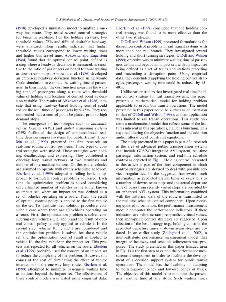
The study presented in this paper is part of a research
in the area of advanced public transportation systems
that include GPS/SO integrated AVL system, real-time
passenger information system, and real-time schedule
control as depicted in Fig. 1. Holding control presentedin this article is part of the third component in which
control strategies are devised to deal with possible ser-
vice irregularities. In the suggested framework, such
information as predicted arrival times of every bus to
a number of downstream stops and the actual departure
time of buses from recently visited stops are provided by
an enhanced AVL system. This information combined
with the historical data of the route is transmitted tothe real time schedule control component. Upon receiv-
ing updated information, the performance measurement
module computes the performance indicators. If these
indicators are below certain pre-specified critical values,
then appropriate control strategies are suggested. Upon
selection of the best strategy (e.g., holding control), the
predicted departure times at downstream stops are up-
dated. In an earlier study (Zolfaghari et al., 2002), amulti-attribute performance measurement model that
integrated headway and schedule adherences was pro-
posed. The study presented in this paper (shaded area
in Fig. 1) is the first step to extend the performance mea-
surement component in order to facilitate the develop-
ment of a decision support system for public transit
operations. The model has the flexibility of adapting
to both high-occupancy and low-occupancy of buses.The objective of this model is to minimize the passen-
gers� waiting time at any stops. Such waiting times
System Monitoringand Control
Process AVL System
HistoricalData
Data Collection Performance Measurement
Selection of Control Strategies
HoldingControl
ControlAction 1
ControlAction n
… …
Fig. 1. Framework of a computer-based real-time schedule control for public transit systems.
102 S. Zolfaghari et al. / International Journal of Transport Management 2 (2004) 99–110
include the waiting time of new arrivals as well as that of
the left-behind passengers. In the model proposed here-
in, the optimization problem is solved simultaneously for
all buses on the route.
The remainder of this paper is organized as follows.Section 2 describes the problem of interest. Section 3
presents the mathematical model. A heuristic approach
used to solve this model is presented in Section 4. Sec-
tion 5 discusses a numerical example. Section 6, is for
the summary and conclusions.
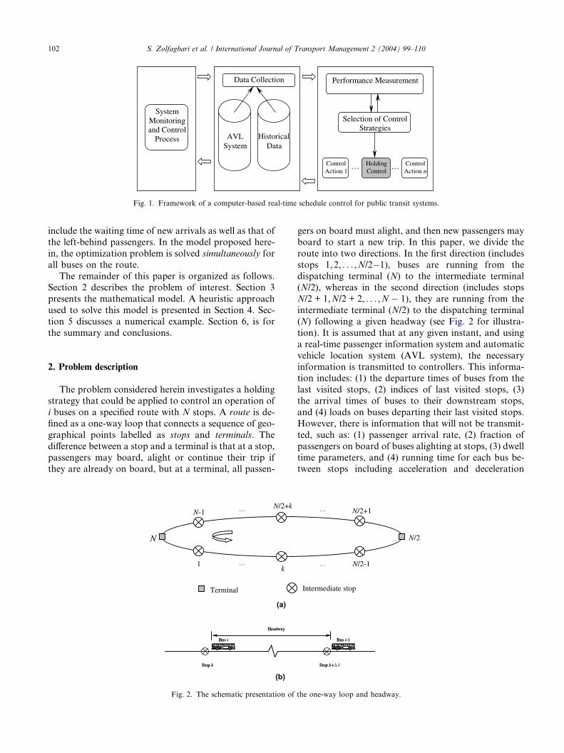
2. Problem description
The problem considered herein investigates a holding
strategy that could be applied to control an operation of
i buses on a specified route with N stops. A route is de-
fined as a one-way loop that connects a sequence of geo-
graphical points labelled as stops and terminals. The
difference between a stop and a terminal is that at a stop,
passengers may board, alight or continue their trip ifthey are already on board, but at a terminal, all passen-
(a)
Stop k
Bus i
Headway
Stop k
Bus i
Headway
(b)
…
N
1
N/2+k N-1
k
…
Terminal
Fig. 2. The schematic presentation of
gers on board must alight, and then new passengers may
board to start a new trip. In this paper, we divide the
route into two directions. In the first direction (includes
stops 1,2, . . . ,N/2�1), buses are running from the
dispatching terminal (N) to the intermediate terminal(N/2), whereas in the second direction (includes stops
N/2 + 1,N/2 + 2, . . . ,N � 1), they are running from the
intermediate terminal (N/2) to the dispatching terminal
(N) following a given headway (see Fig. 2 for illustra-
tion). It is assumed that at any given instant, and using
a real-time passenger information system and automatic
vehicle location system (AVL system), the necessary
information is transmitted to controllers. This informa-tion includes: (1) the departure times of buses from the
last visited stops, (2) indices of last visited stops, (3)
the arrival times of buses to their downstream stops,
and (4) loads on buses departing their last visited stops.
However, there is information that will not be transmit-
ted, such as: (1) passenger arrival rate, (2) fraction of
passengers on board of buses alighting at stops, (3) dwell
time parameters, and (4) running time for each bus be-tween stops including acceleration and deceleration
Bus i-1
Stop k+
Bus i-1
Stop k+∆ k
N/2-1
N/2+1
N/2
…
…
Intermediate stop
the one-way loop and headway.
S. Zolfaghari et al. / International Journal of Transport Management 2 (2004) 99–110 103
times. We assume that these parameters could be deter-
mined from available historical data.
2.1. Assumptions and limitations
The model is subject to the following assumptionsand limitations:
Assumptions:
• When the bus is not loaded to capacity, it is assumedthat all boarding takes place at the front door and
alighting takes place at the rear door.
• When the bus is loaded to capacity, the front door
can be used for both boarding and alighting. In such
cases, boarding can only start when front-door
alighting is completed.
Limitations:
• Running times are approximated by their expected
values.
• Dwell time function is approximated by a linear
function.
• During controlling the vehicles we consider a limited
number of downstream stops for each bus, which is
called ‘‘rolling horizon’’.
2.2. Data requirements
In this paper, it is assumed that the following infor-
mation is either available or could be estimated: Pro-
vided by an AVL system:
• Actual departure times of buses from the most
recently visited stops.
• Predicted arrival times of buses from downstream
stops (maximum eN istops for each bus i).
Estimated from historical data:
• Expected value of bus running times between stops.
• Expected value of bus dwell times at stops.
• Passenger arrival rates and alighting fractions at each
stop.
• Dwell time function parameters.
2.3. Notation list
The following variables and parameters are used in
the proposed formulations:
i index of vehicles, i = 1, . . . , Ik index of stops, k = 1, . . . ,Ndi,k departure time of bus i from stop k
Fi,k predicted arrival time of bus i at stop k
li,k load in bus i departing stop k
pi,k passengers left behind by bus i at stop k
Di,k demand for bus i at stop k
rk passenger arrival rate at stop k
vi,k 1, if bus i is loaded to capacity when it departstop k; 0, otherwise
Sui;k dwell time of bus i at stop k when the passenger
load is below the bus capacity
Sci;k dwell time of bus i at stop k when bus i is loaded
to capacity
Cj dwell time function parameter
Qk passenger alighting fraction at stop k
Afk passenger alighting fraction at stop k that use
the front door for alighting
Ark passenger alighting fraction at stop k that use
the rear door for alighting
Rk running time from stop k-1 to stop k, including
acceleration and deceleration
Lmax passenger capacity of bus
Mj sufficiently large numbers
K set of stations on the route K = {1,2,3, . . . ,N/2, . . . ,N}
I set of buses operating on the route
I = {1,2,3, . . . , i, . . . , I}eN itotal number of stops in the horizon of bus i
Th rolling horizon
g expected value of running times on a route
u expected value of bus dwell time at stops
tnow present time (time now)li index of the last visited stop by bus i
kfst the first stop in the horizon of bus i
2.4. Rolling horizon
As discussed above, the transit system considered in
this study is a one-way loop in which buses are operating
on the route following a planned headway. When con-
trolling the route, and for each bus, only a limited num-
ber of immediate downstream stops are considered. Thisway, the problem could be reduced to a reasonable size
if there are a large number of stops and buses on the
route. The number of downstream stops, eN i, depends
on the length of the rolling horizon T h as described in
Fig. 3. The rolling horizon is a common term in many
fields that could be defined differently depending on
the application (e.g., Newell, 1998; Choong et al.,
2001). In this paper, the rolling horizon is defined as areasonable length of time in which bus movement on
the route could be projected fairly. It is a ‘‘horizon’’ as
it is a finite future time period, and it is ‘‘rolling’’ be-
cause it moves forward as buses progress on their routes.
Since stops are not equidistant, then the total number of
stops in a given rolling horizon could differ for each bus
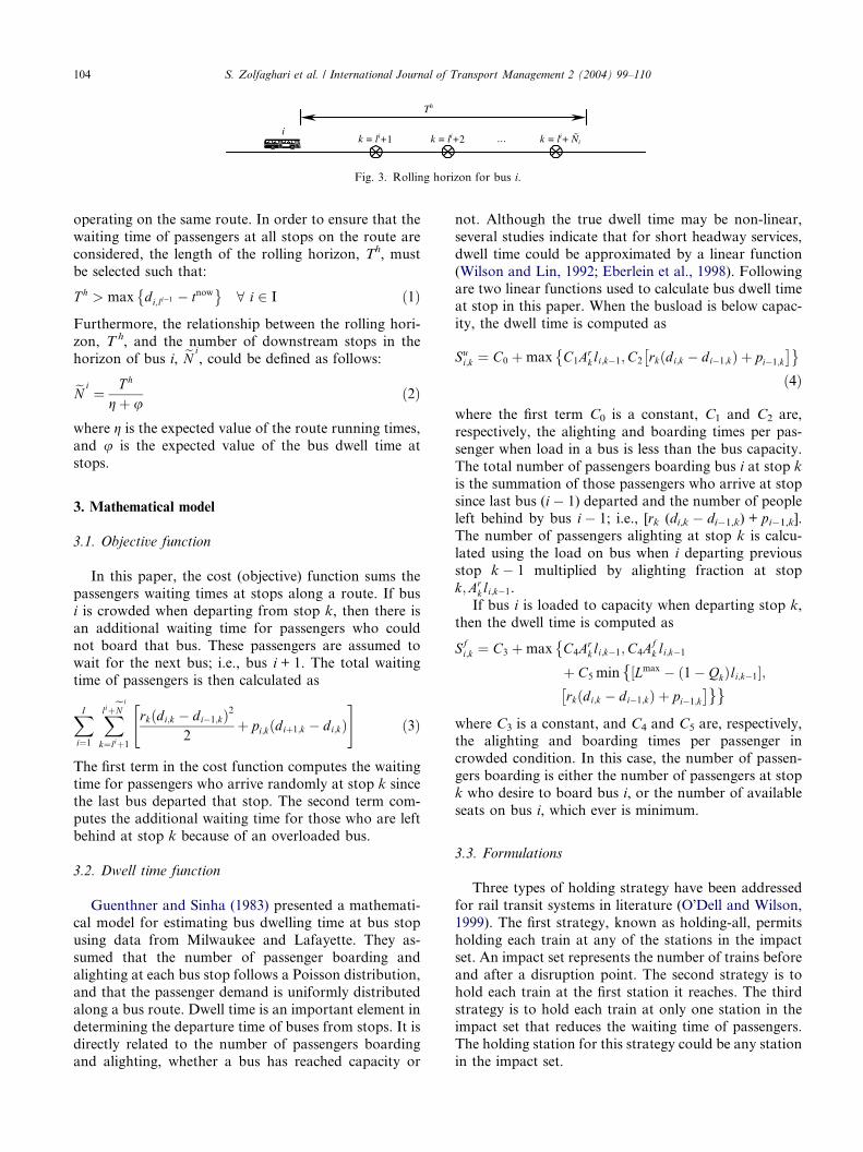
Th
k = li+1 k = li+2 k = li+ Ñi
i…
Fig. 3. Rolling horizon for bus i.
104 S. Zolfaghari et al. / International Journal of Transport Management 2 (2004) 99–110
operating on the same route. In order to ensure that the
waiting time of passengers at all stops on the route are
considered, the length of the rolling horizon, Th, must
be selected such that:
T h > max di;li�1 � tnow� �
8 i 2 I ð1Þ
Furthermore, the relationship between the rolling hori-
zon, T h, and the number of downstream stops in the
horizon of bus i, eN i, could be defined as follows:
eN i ¼ T h
gþ uð2Þ
where g is the expected value of the route running times,
and u is the expected value of the bus dwell time at
stops.
3. Mathematical model
3.1. Objective function
In this paper, the cost (objective) function sums the
passengers waiting times at stops along a route. If bus
i is crowded when departing from stop k, then there is
an additional waiting time for passengers who could
not board that bus. These passengers are assumed towait for the next bus; i.e., bus i + 1. The total waiting
time of passengers is then calculated as
XI
i¼1
XliþeN i
k¼liþ1
rkðdi;k � di�1;kÞ2
2þ pi;k diþ1;k � di;kð Þ
" #ð3Þ
The first term in the cost function computes the waitingtime for passengers who arrive randomly at stop k since
the last bus departed that stop. The second term com-
putes the additional waiting time for those who are left
behind at stop k because of an overloaded bus.
3.2. Dwell time function
Guenthner and Sinha (1983) presented a mathemati-cal model for estimating bus dwelling time at bus stop
using data from Milwaukee and Lafayette. They as-
sumed that the number of passenger boarding and
alighting at each bus stop follows a Poisson distribution,
and that the passenger demand is uniformly distributed
along a bus route. Dwell time is an important element in
determining the departure time of buses from stops. It is
directly related to the number of passengers boardingand alighting, whether a bus has reached capacity or
not. Although the true dwell time may be non-linear,
several studies indicate that for short headway services,
dwell time could be approximated by a linear function
(Wilson and Lin, 1992; Eberlein et al., 1998). Following
are two linear functions used to calculate bus dwell timeat stop in this paper. When the busload is below capac-
ity, the dwell time is computed as
Sui;k ¼ C0 þmax C1A
rkli;k�1;C2 rkðdi;k � di�1;kÞ þ pi�1;k
� �� �ð4Þ
where the first term C0 is a constant, C1 and C2 are,
respectively, the alighting and boarding times per pas-
senger when load in a bus is less than the bus capacity.
The total number of passengers boarding bus i at stop k
is the summation of those passengers who arrive at stop
since last bus (i � 1) departed and the number of peopleleft behind by bus i � 1; i.e., [rk (di,k � di�1,k) + pi�1,k].
The number of passengers alighting at stop k is calcu-
lated using the load on bus when i departing previous
stop k � 1 multiplied by alighting fraction at stop
k;Arkli;k�1.
If bus i is loaded to capacity when departing stop k,
then the dwell time is computed as
Sfi;k ¼ C3 þmax C4A
rkli;k�1;C4A
fk li;k�1
�þ C5 minf Lmax � ð1� QkÞli;k�1½ �;rkðdi;k � di�1;kÞ þ pi�1;k
� �ggwhere C3 is a constant, and C4 and C5 are, respectively,the alighting and boarding times per passenger in
crowded condition. In this case, the number of passen-
gers boarding is either the number of passengers at stop
k who desire to board bus i, or the number of available
seats on bus i, which ever is minimum.
3.3. Formulations
Three types of holding strategy have been addressed
for rail transit systems in literature (O�Dell and Wilson,
1999). The first strategy, known as holding-all, permits
holding each train at any of the stations in the impact
set. An impact set represents the number of trains before
and after a disruption point. The second strategy is to
hold each train at the first station it reaches. The third
strategy is to hold each train at only one station in theimpact set that reduces the waiting time of passengers.
The holding station for this strategy could be any station
in the impact set.
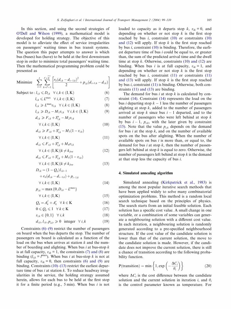
S. Zolfaghari et al. / International Journal of Transport Management 2 (2004) 99–110 105
In this section, and using the second strategies of
O�Dell and Wilson (1999), a mathematical model is
developed for holding strategy. The objective of this
model is to alleviate the effect of service irregularities
on passengers� waiting times in bus transit systems.
The question this paper attempts to answer is whichbus (buses) has (have) to be held at the first downstream
stop in order to minimize total passengers� waiting time.
Then the mathematical programming problem could be
presented as
MinimizeXI
i¼1
XliþeN i
k¼liþ1
rkðdi;k � di�1;kÞ2
2þ pi;kðdiþ1;k � di;kÞ
" #Subject to : li;k 6Di;k 8 i;k 2 ðI;KÞ ð6Þ
li;k 6 Lmax 8 i;k 2 ðI;KÞ ð7Þli;k P Lmaxvi;k 8 i;k 2 ðI;KÞ ð8Þli;k PDi;k �M1vi;k 8 i;k 2 ðI;KÞ ð9Þdi;k P F i;k þ Su
i;k �M2vi;k
8 i;k 2 ðI;KÞ ð10Þdi;k P F i;k þ Sc
i;k �M3ð1� vi;kÞ8 i;k 2 ðI;KÞ ð11Þ
di;k 6 F i;k þ Sui;k þM4vi;k
8 i;k 2 ðI;KÞjk 6¼ kfrst ð12Þdi;k 6 F i;k þ Sc
i;k þM5ð1� vi;kÞ8 i;k 2 ðI;KÞjk 6¼ kfrst ð13Þ
Di;k ¼ ð1�QkÞli;k�1
þ rkðdi;k � di�1;kÞþ pi�1;k
8 i;k 2 ðI;KÞ ð14Þpi;k ¼max 0;Di;k � Lmaxf g8 i;k 2 ðI;KÞ ð15Þ
Qk ¼ Afk þAr
k 8 k 2K ð16Þ06Qk 6 1 8 k 2K ð17Þvi;k 2 0;1f g 8 i;k ð18Þdi;k; li;k;pi;k;P 0 integer 8 i;k ð19Þ
Constraints (6)–(9) restrict the number of passengers
on board when the bus departs the stop. The number of
passengers on board is calculated as a function of the
load on the bus when arrives at station k and the num-
ber of boarding and alighting. When bus i at bus-stop k
is at full capacity, vik = 1, the constraints (7) and (8) are
binding (li,k = lmax). When bus i at bus-stop k is not at
full capacity, vik = 0, then constraints (6) and (9) are
binding. Constraints (10)–(13) restrict the earliest depar-
ture time of bus i at station k. To reduce headway irreg-
ularities in the service, the holding strategy assumed
herein, allows for each bus to be held at the first stop
it for a finite period (e.g., 5 min). When bus i is not
loaded to capacity as it departs stop k, vik = 0, and
depending on whether or not stop k is the first stop
reached by bus i, constraint (10) or constraints (10)
and (12) will apply. If stop k is the first stop reached
by bus i, constraint (10) is binding. Therefore, the earli-
est departure time of bus i could be equal to, or greaterthan, the sum of the predicted arrival time and the dwell
time at stop k. Otherwise, constraints (10) and (12) are
binding. When bus i is at full capacity, vik = 1, and
depending on whether or not stop k is the first stop
reached by bus i, constraint (11) or constraints (11)
and (13) will apply. If stop k is the first stop reached
by bus i, constraint (11) is binding. Otherwise, both con-
straints (11) and (13) are binding.The demand for bus i at stop k is calculated by con-
straint (14). Constraint (14) represents the load on the
bus i departing stop k � 1 less the number of passengers
alighting at stop k, added to the number of passengers
arrived at stop k since bus i � 1 departed, and to the
number of passengers who were left behind at stop k
by bus i � 1, pi,k, with the later given by constraint
(15). Note that the value pi,k depends on the demandfor bus i at the stop k, and on the number of available
spots on the bus after alighting. When the number of
available spots on bus i is more than, or equal to, the
demand for bus i at stop k, then the number of passen-
gers left behind at stop k is equal to zero. Otherwise, the
number of passengers left behind at stop k is the demand
at that stop less the capacity of bus i.
4. Simulated annealing algorithm
Simulated annealing (Kirkpatrick et al., 1983) is
among the most popular iterative search methods that
have been applied widely to solve many combinatorial
optimization problems. This method is a random local
search technique based on the principles of physics.The search starts from an initial feasible solution. Each
solution has a specific cost value. A small change in one
variable, or a combination of some variables can gener-
ate a neighbouring solution with a different cost value.
In each iteration, a neighbouring solution is randomly
generated according to a pre-specified neighbourhood
structure. If the cost value of the candidate solution is
lower than that of the current solution, the move tothe candidate solution is made. However, if the candi-
date does not improve the current solution, there is still
a chance of transition according to the following proba-
bility function.
PðtransitionÞ ¼ min 1; exp �DCi
hi
� �� �ð20Þ
where DCi is the cost difference between the candidate
solution and the current solution in iteration i, and hiis the control parameter known as temperature. For
106 S. Zolfaghari et al. / International Journal of Transport Management 2 (2004) 99–110
each iteration, the above transition probability value is
compared to a uniform random number generated. If
the transition probability value is greater than or equal
to the value of random number generated, then the tran-
sition to the worse solution is accepted, otherwise the
transition from the current solution to the candidatesolution is rejected. Then, another solution in the neigh-
bourhood of the current solution will be generated and
evaluated. The temperature hi has a significant impact
on the transition probability. The greater the tempera-
ture, the higher the probability will be. In a standard
simulated annealing, the initial temperature is usually
set at a high level to allow the search to move freely to
worse solutions. As the search continues, the tempera-ture declines according to a cooling schedule. Toward
the end of the search process, it is less likely to move
to a worse neighbouring solution. The change in temper-
ature values is controlled by a cooling schedule. To se-
lect a cooling schedule, it is necessary to decide on the
type of the algorithm, homogenous or inhomogeneous.
In a homogeneous algorithm, the value of temperature
remains constant for a certain number of iterationsand then is decreased in between subsequent chains.
However, in an inhomogeneous algorithm, the value
of the temperature is decreased between subsequent
transitions (Van Laarhoven and Aarts, 1987). The
asymptotic convergence of both types has been well
studied in the literature (Van Laarhoven and Aarts,
1987), (Gidas, 1985), and (Hajek, 1988).
In this paper we adopt an inhomogeneous approachand we use an adaptive cooling schedule that may occa-
sionally increase the temperature according to the char-
acteristics of the search trajectory as follows.
h ¼ h þ k lnð1þ r Þ ð21Þ
i min iFig. 4. Stop and bus positions f
where hmin is the minimum temperature value, k is a coef-ficient that controls the rate of temperature rise, and ri is
the number of consecutive upward moves at iteration i.
The initial value of ri is zero, thus the initial temperature
h0 = hmin. At any point during the search, if a move is
made to a solution with a cost higher than that of the pre-vious solution (i.e., upward move), then the counter riincremented by 1. If the new solution has an equal cost,
ri remains unchanged; and if the cost is improved, then riis reset to zero. The two other main elements of any sim-
ulated annealing base algorithm are cost function and
neighbourhood generating mechanism. For the problem
described in Section 3, the cost function is defined as the
total passenger waiting time and a neighbour is gener-ated by adding/deducting a prescribed holding value to/
from the departure time of a randomly selected bus.
The heuristic used in this paper is explained in the
Appendix A. The algorithm was coded in Visual Basic
and implemented on a Pentium III with 450 MHz CPU.
5. Numerical example
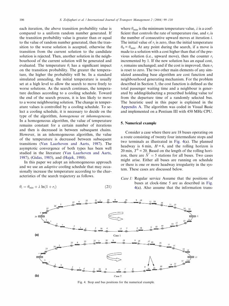
Consider a case where there are 18 buses operating on
a route consisting of twenty four intermediate stops and
two terminals as illustrated in Fig. 4(a). The planned
headway is 6 min, H = 6, and the rolling horizon is
20 min, Th = 20. Based on the length of the rolling hori-
zon, there are eN i ¼ 5 stations for all buses. Two cases
might arise. Either all buses are running on scheduleor there is one or more headway irregularity in the sys-
tem. These cases are discussed below.
Case 1: Regular service Assume that the positions of
buses at clock-time 5 are as described in Fig.
4(a). Also assume that the information trans-
or the numerical example.
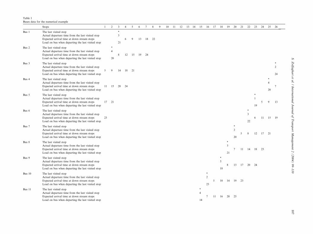
Table 1
Buses data for the numerical example
Stops 1 2 3 4 5 6 7 8 9 10 11 12 13 14 15 16 17 18 19 20 21 22 23 24 25 26
Bus 1 The last visited stop *
Actual departure time from the last visited stop 3
Expected arrival time at down stream stops 6 9 13 18 22
Load on bus when departing the last visited stop 21
Bus 2 The last visited stop *
Actual departure time from the last visited stop 4
Expected arrival time at down stream stops 8 12 15 19 24
Load on bus when departing the last visited stop 20
Bus 3 The last visited stop *
Actual departure time from the last visited stop 2
Expected arrival time at down stream stops 5 9 14 18 21
Load on bus when departing the last visited stop 24
Bus 4 The last visited stop *
Actual departure time from the last visited stop 4
Expected arrival time at down stream stops 11 15 20 24 7
Load on bus when departing the last visited stop 20
Bus 5 The last visited stop *
Actual departure time from the last visited stop 1
Expected arrival time at down stream stops 17 21 5 9 13
Load on bus when departing the last visited stop 19
Bus 6 The last visited stop *
Actual departure time from the last visited stop 3
Expected arrival time at down stream stops 23 6 11 15 19
Load on bus when departing the last visited stop 22
Bus 7 The last visited stop *
Actual departure time from the last visited stop 2
Expected arrival time at down stream stops 5 8 12 17 21
Load on bus when departing the last visited stop 20
Bus 8 The last visited stop *
Actual departure time from the last visited stop 3
Expected arrival time at down stream stops 7 11 14 18 23
Load on bus when departing the last visited stop 21
Bus 9 The last visited stop *
Actual departure time from the last visited stop 5
Expected arrival time at down stream stops 8 13 17 20 24
Load on bus when departing the last visited stop 18
Bus 10 The last visited stop *
Actual departure time from the last visited stop 2
Expected arrival time at down stream stops 5 10 14 19 23
Load on bus when departing the last visited stop 23
Bus 11 The last visited stop *
Actual departure time from the last visited stop 4
Expected arrival time at down stream stops 7 11 16 20 25
Load on bus when departing the last visited stop 14
S.Zolfa
ghariet
al./Intern
atio
nalJournalofTransport
Managem
ent2(2004)99–110
107
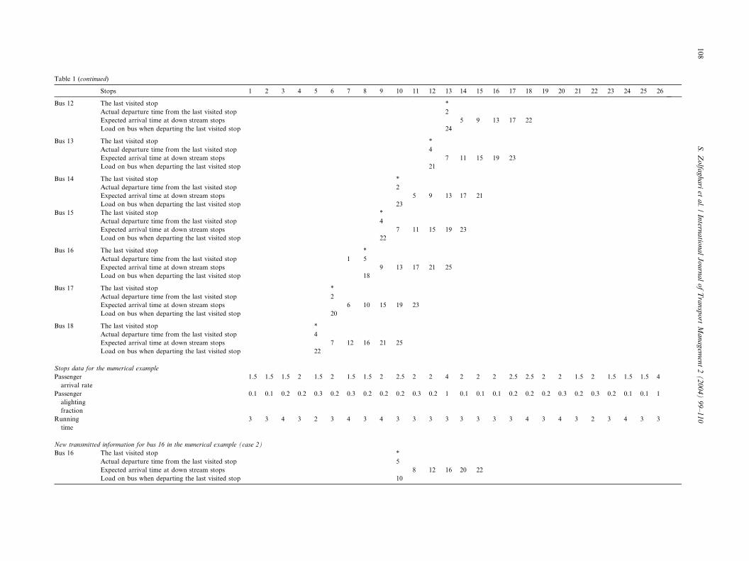
Table 1 (continued)
Stops 1 2 3 4 5 6 7 8 9 10 11 12 13 14 15 16 17 18 19 20 21 22 23 24 25 26
Bus 12 The last visited stop *
Actual departure time from the last visited stop 2
Expected arrival time at down stream stops 5 9 13 17 22
Load on bus when departing the last visited stop 24
Bus 13 The last visited stop *
Actual departure time from the last visited stop 4
Expected arrival time at down stream stops 7 11 15 19 23
Load on bus when departing the last visited stop 21
Bus 14 The last visited stop *
Actual departure time from the last visited stop 2
Expected arrival time at down stream stops 5 9 13 17 21
Load on bus when departing the last visited stop 23
Bus 15 The last visited stop *
Actual departure time from the last visited stop 4
Expected arrival time at down stream stops 7 11 15 19 23
Load on bus when departing the last visited stop 22
Bus 16 The last visited stop *
Actual departure time from the last visited stop 1 5
Expected arrival time at down stream stops 9 13 17 21 25
Load on bus when departing the last visited stop 18
Bus 17 The last visited stop *
Actual departure time from the last visited stop 2
Expected arrival time at down stream stops 6 10 15 19 23
Load on bus when departing the last visited stop 20
Bus 18 The last visited stop *
Actual departure time from the last visited stop 4
Expected arrival time at down stream stops 7 12 16 21 25
Load on bus when departing the last visited stop 22
Stops data for the numerical example
Passenger
arrival rate
1.5 1.5 1.5 2 1.5 2 1.5 1.5 2 2.5 2 2 4 2 2 2 2.5 2.5 2 2 1.5 2 1.5 1.5 1.5 4
Passenger
alighting
fraction
0.1 0.1 0.2 0.2 0.3 0.2 0.3 0.2 0.2 0.2 0.3 0.2 1 0.1 0.1 0.1 0.2 0.2 0.2 0.3 0.2 0.3 0.2 0.1 0.1 1
Running
time
3 3 4 3 2 3 4 3 4 3 3 3 3 3 3 3 3 4 3 4 3 2 3 4 3 3
New transmitted information for bus 16 in the numerical example (case 2)
Bus 16 The last visited stop *
Actual departure time from the last visited stop 5
Expected arrival time at down stream stops 8 12 16 20 22
Load on bus when departing the last visited stop 10
108
S.Zolfa
ghariet
al./Intern
atio
nalJournalofTransport
Managem
ent2(2004)99–110
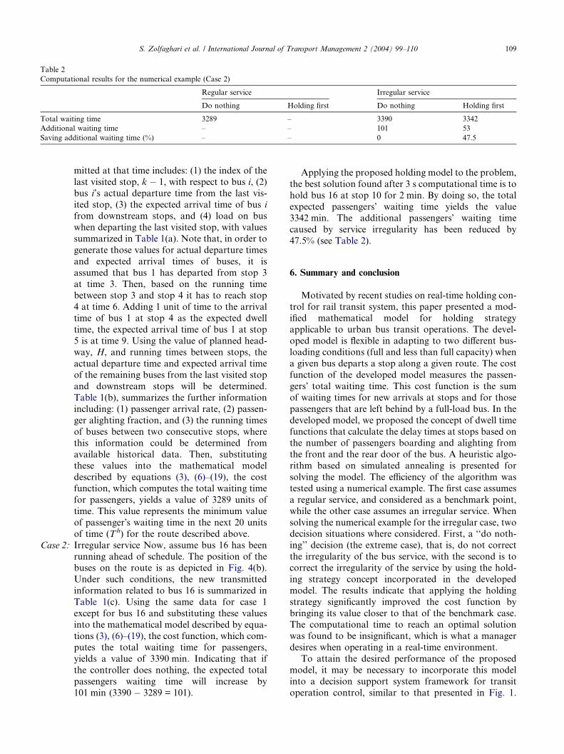
Table 2
Computational results for the numerical example (Case 2)
Regular service Irregular service
Do nothing Holding first Do nothing Holding first
Total waiting time 3289 – 3390 3342
Additional waiting time – – 101 53
Saving additional waiting time (%) – – 0 47.5
S. Zolfaghari et al. / International Journal of Transport Management 2 (2004) 99–110 109
mitted at that time includes: (1) the index of the
last visited stop, k � 1, with respect to bus i, (2)bus i’s actual departure time from the last vis-
ited stop, (3) the expected arrival time of bus i
from downstream stops, and (4) load on bus
when departing the last visited stop, with values
summarized in Table 1(a). Note that, in order to
generate those values for actual departure times
and expected arrival times of buses, it is
assumed that bus 1 has departed from stop 3at time 3. Then, based on the running time
between stop 3 and stop 4 it has to reach stop
4 at time 6. Adding 1 unit of time to the arrival
time of bus 1 at stop 4 as the expected dwell
time, the expected arrival time of bus 1 at stop
5 is at time 9. Using the value of planned head-
way, H, and running times between stops, the
actual departure time and expected arrival timeof the remaining buses from the last visited stop
and downstream stops will be determined.
Table 1(b), summarizes the further information
including: (1) passenger arrival rate, (2) passen-
ger alighting fraction, and (3) the running times
of buses between two consecutive stops, where
this information could be determined from
available historical data. Then, substitutingthese values into the mathematical model
described by equations (3), (6)–(19), the cost
function, which computes the total waiting time
for passengers, yields a value of 3289 units of
time. This value represents the minimum value
of passenger�s waiting time in the next 20 units
of time (Th) for the route described above.
Case 2: Irregular service Now, assume bus 16 has beenrunning ahead of schedule. The position of the
buses on the route is as depicted in Fig. 4(b).
Under such conditions, the new transmitted
information related to bus 16 is summarized in
Table 1(c). Using the same data for case 1
except for bus 16 and substituting these values
into the mathematical model described by equa-
tions (3), (6)–(19), the cost function, which com-putes the total waiting time for passengers,
yields a value of 3390 min. Indicating that if
the controller does nothing, the expected total
passengers waiting time will increase by
101 min (3390 � 3289 = 101).
Applying the proposed holding model to the problem,
the best solution found after 3 s computational time is to
hold bus 16 at stop 10 for 2 min. By doing so, the total
expected passengers� waiting time yields the value
3342 min. The additional passengers� waiting time
caused by service irregularity has been reduced by
47.5% (see Table 2).
6. Summary and conclusion
Motivated by recent studies on real-time holding con-
trol for rail transit system, this paper presented a mod-
ified mathematical model for holding strategy
applicable to urban bus transit operations. The devel-
oped model is flexible in adapting to two different bus-loading conditions (full and less than full capacity) when
a given bus departs a stop along a given route. The cost
function of the developed model measures the passen-
gers� total waiting time. This cost function is the sum
of waiting times for new arrivals at stops and for those
passengers that are left behind by a full-load bus. In the
developed model, we proposed the concept of dwell time
functions that calculate the delay times at stops based onthe number of passengers boarding and alighting from
the front and the rear door of the bus. A heuristic algo-
rithm based on simulated annealing is presented for
solving the model. The efficiency of the algorithm was
tested using a numerical example. The first case assumes
a regular service, and considered as a benchmark point,
while the other case assumes an irregular service. When
solving the numerical example for the irregular case, twodecision situations where considered. First, a ‘‘do noth-
ing’’ decision (the extreme case), that is, do not correct
the irregularity of the bus service, with the second is to
correct the irregularity of the service by using the hold-
ing strategy concept incorporated in the developed
model. The results indicate that applying the holding
strategy significantly improved the cost function by
bringing its value closer to that of the benchmark case.The computational time to reach an optimal solution
was found to be insignificant, which is what a manager
desires when operating in a real-time environment.
To attain the desired performance of the proposed
model, it may be necessary to incorporate this model
into a decision support system framework for transit
operation control, similar to that presented in Fig. 1.
110 S. Zolfaghari et al. / International Journal of Transport Management 2 (2004) 99–110
The holding strategy model proposed in this paper is a
first step in extending previously developed performance
monitoring modules to include control actions. This
model is capable of solving the problem simultaneously
for all buses on the route. This is considered as an
important aspect of the model presented herein as com-pared to previously developed models. The implementa-
tion, however, would be more effective if it is in
conjunction with other control strategies. This is impor-
tant since different services are subject to different
behavioural interruptions, thus requiring the implemen-
tation of different control strategies. For example, there
are cases where buses might be early while other buses
late. An early bus requires a decelerating action (e.g.,holding), while a late bus requires an accelerating action
(e.g., stop-skipping). Further research is still needed in
this direction to develop other control strategies for
urban transit operations. Such strategies may include
short-turning, stop-skipping, dead-heading, expressing,
adding/removing a trip and signal priority.
Acknowledgments
The authors wish to thank anonymous reviewers for
their valuable suggestions. The financial support of the
Geomatics for Informed Decision (GEOIDE) Network
of Centres of Excellence (Grant TCO#51) is also greatly
appreciated.
Appendix A. SA algorithm
Step 1:
Set i = 1 and select hmin
Select an initial solution and set the current solu-
tion Bi and the best solution Oi equal
to the initial solution.Step 2:
Select a candidate solution Bc from the neighbour-
hood of Bi
IF Z(Bc) < Z(Bi) THEN
Set Bi+1 = Bc
IF Z(Bc) < Z(Oi) THEN set Oi = Bc.
Go to Step 3
END IFGenerate a random number u from a U(0,1)
distribution;
Compute the transition probability P(Bi,Bc) =
exp[(Z(Bi) � Z(Bc))/hi]IF u 6 P(Bi,B
c), THEN set Bi+1 = Bc.
Step 3:
Select hi+1Set i = i + 1.
IF termination condition is satisfied, THEN stop;
ELSE, go to Step 2.
END
References
Abkowitz, M.D., Engelstein, I., 1984. Methods for maintaining transit
service regularity. Transportation Research Record 961, 1–8.
Abkowitz, M.D., Eiger, A., Engelstein, I., 1986. Optimal headway
variation on transit routes. Journal of Advanced Transportation 20
(1), 73–88.
Barnett, A.I., 1974. On controlling randomness in transit operations.
Transportation Science 8 (2), 101–116.
Choong, S., Cole, M.H., Kutanoglu, E., 2001. Empty Container
Management for Container-on-Barge (COB) Transportation:
Planning Horizon Effects on Empty Container Management in a
Multi-Modal Transportation Network, MBTC-2003, Mack-Black-
well Transportation Center, University of Arkansas, Fayetteville,
Arkansas.
Eberlein, X.J., Wilson, M.H.M., Barnhart, C., Bernstein, D., 1998.
The real-time deadheading problem in transit operations control.
Transportation Research—Part B 32 (2), 77–100.
Eberlein, X., Wilson, N.H.M., Bernstein, D., 1999. Modeling real-time
control strategies in public transit operations. In: Wilson, N.H.M.
(Ed.), Lecture Note in Economics and Mathematical Systems No.
471: Computer Aided Transit Scheduling. Springer-Verlag, Berlin,
Heidelberg, pp. 325–346.
Gidas, B., 1985. Non-stationary Markov chains and convergence of
the annealing algorithm. Journal of Statistical Physics 39, 73–131.
Guenthner, R.P., Sinha, K.C., 1983. Modeling bus delay due to
passenger boarding and alighting. Transportation Research
Record 915, 7–13.
Hajek, B., 1988. Cooling schedules for optimal annealing. Mathemat-
ics of Operations Research 13 (2), 311–329.
Kirkpatrick, S., Gelatt Jr., C.D., Vecchi, M.P., 1983. Optimization by
simulated annealing. Science 220 (4598), 671–680.
Koffman, D., 1978. A simulation study of alternative real-time bus
headway control strategies. Transportation Research Record 663,
41–46.
Newell, G.F., 1998. The rolling horizon scheme of traffic signal
control. Transportation Research–Part A 32, 39–44.
O�Dell, S.W., Wilson, N.H.M., 1999. Optimal real-time control
strategies for rail transit operations during disruptions. In: Wilson,
N.H.M. (Ed.), Lecture Notes in Economics and Mathematical
Systems No. 471: Computer-aided Scheduling. Springer-Verlag,
pp. 299–323.
Osuna, E.E., Newell, G.F., 1972. Control strategies for an idealized
public transportation system. Transportation Science 16 (1), 52–72.
Turnquist, M.A., 1978. Strategies for improving reliability of bus
transit service. Transportation Research Record 818, 7–13.
Turnquist, M.A., Blume, S.W., 1980. Evaluating potential effectiveness
of headway control strategies for transit systems. Transportation
Research Record 746, 25–29.
Van Laarhoven, P.J.M., Aarts, E.H.L., 1987. Simulated Annealing:
Theory and Applications. Kluwer, Dordrecht.
Wilson, N.H.M., Lin, T., 1992. Dwell time relationships for light rail
systems. Transportation Research Record 1361, 287–295.
Zolfaghari, S., Jaber, M.Y., Azizi, N., 2002. A multi-attribute
performance measurement model for advanced public transit
systems. Intelligent Transportation Systems Journal 7 (3–4), 295–
314.