MSc thesis

Master’s Programme in Computer Science

A Method for Wavelet-Based Time SeriesAnalysis of Historical Newspapers

Jari Avikainen

December 3, 2019

Faculty of ScienceUniversity of Helsinki

Supervisor(s)

Prof. Hannu Toivonen

Examiner(s)

Prof. Hannu Toivonen, Dr. Lidia Pivovarova

Contact information

P. O. Box 68 (Pietari Kalmin katu 5)00014 University of Helsinki,Finland

Email address: info@cs.helsinki.fiURL: http://www.cs.helsinki.fi/

Faculty of Science Master’s Programme in Computer Science

Jari Avikainen

A Method for Wavelet-Based Time Series Analysis of Historical Newspapers

Prof. Hannu Toivonen

MSc thesis December 3, 2019 43 pages

historical newspapers, wavelet transform, step detection

Helsinki University Library

Algorithms study track

This thesis presents a wavelet-based method for detecting moments of fast change in the textualcontents of historical newspapers. The method works by generating time series of the relativefrequencies of different words in the newspaper contents over time, and calculating their wavelettransforms. Wavelet transform is essentially a group of transformations describing the changeshappening in the original time series at different time scales, and can therefore be used topinpoint moments of fast change in the data. The produced wavelet transforms are then usedto detect fast changes in word frequencies by examining products of multiple scales of thetransform.

The properties of the wavelet transform and the related multi-scale product are evaluated inrelation to detecting various kinds of steps and spikes in different noise environments. Thesuitability of the method for analysing historical newspaper archives is examined using anexample corpus consisting of 487 issues of Uusi Suometar from 1869–1918 and 250 issues ofWiipuri from 1893–1918. Two problematic features in the newspaper data, noise caused byOCR (optical character recognition) errors and uneven temporal distribution of the data, areidentified and their effects on the results of the presented method are evaluated using syntheticdata. Finally, the method is tested using the example corpus, and the results are examinedbriefly.

The method is found to be adversely affected especially by the uneven temporal distribution ofthe newspaper data. Without additional processing, or improving the quality of the examineddata, a significant amount of the detected steps are due to the noise in the data. Various waysof alleviating the effect are proposed, among other suggested improvements on the system.

ACM Computing Classification System (CCS)Information systems → Information retrieval → Retrieval tasks and goals → InformationextractionGeneral and reference → Cross-computing tools and techniques → Evaluation

HELSINGIN YLIOPISTO – HELSINGFORS UNIVERSITET – UNIVERSITY OF HELSINKITiedekunta — Fakultet — Faculty Koulutusohjelma — Utbildningsprogram — Study programme

Tekija — Forfattare — Author

Tyon nimi — Arbetets titel — Title

Ohjaajat — Handledare — Supervisors

Tyon laji — Arbetets art — Level Aika — Datum — Month and year Sivumaara — Sidoantal — Number of pages

Tiivistelma — Referat — Abstract

Avainsanat — Nyckelord — Keywords

Sailytyspaikka — Forvaringsstalle — Where deposited

Muita tietoja — ovriga uppgifter — Additional information

Contents

1 Introduction 11.1 Background . . . . . . . . . . . . . . . . . . . . . . . . . . . . . . . . . . . 11.2 Event detection in media . . . . . . . . . . . . . . . . . . . . . . . . . . . . 21.3 Step detection using wavelet analysis . . . . . . . . . . . . . . . . . . . . . 31.4 Thesis structure . . . . . . . . . . . . . . . . . . . . . . . . . . . . . . . . . 4

2 Wavelet analysis 62.1 What is a wavelet transform . . . . . . . . . . . . . . . . . . . . . . . . . . 62.2 Continuous wavelet transform . . . . . . . . . . . . . . . . . . . . . . . . . 62.3 Discrete wavelet transform . . . . . . . . . . . . . . . . . . . . . . . . . . . 82.4 Fast Wavelet Transform . . . . . . . . . . . . . . . . . . . . . . . . . . . . 9

3 A method for event detection using wavelet transforms 133.1 Time-series generation . . . . . . . . . . . . . . . . . . . . . . . . . . . . . 133.2 Wavelet transform . . . . . . . . . . . . . . . . . . . . . . . . . . . . . . . 143.3 Wavelet product . . . . . . . . . . . . . . . . . . . . . . . . . . . . . . . . . 163.4 Problems near the ends of the signal . . . . . . . . . . . . . . . . . . . . . 183.5 Step detection and evaluation . . . . . . . . . . . . . . . . . . . . . . . . . 193.6 Event detection . . . . . . . . . . . . . . . . . . . . . . . . . . . . . . . . . 21

4 Empirical evaluation 234.1 The corpus used for testing the method . . . . . . . . . . . . . . . . . . . . 234.2 Testing the method . . . . . . . . . . . . . . . . . . . . . . . . . . . . . . . 25

4.2.1 Properties of the multiscale product . . . . . . . . . . . . . . . . . . 254.2.2 The effects of noise on the step detection . . . . . . . . . . . . . . . 254.2.3 The effect of data coverage on the step counts . . . . . . . . . . . . 274.2.4 The effect of OCR errors to the step counts . . . . . . . . . . . . . 28

5 Results 29

5.1 Properties of the multiscale product . . . . . . . . . . . . . . . . . . . . . . 295.2 The effects of noise on the step detection . . . . . . . . . . . . . . . . . . . 305.3 The effect of data coverage on the step counts . . . . . . . . . . . . . . . . 325.4 Performance of the event detection . . . . . . . . . . . . . . . . . . . . . . 35

6 Discussion 366.1 Effects of noise and missing data on the system . . . . . . . . . . . . . . . 366.2 Alleviating the effects of uneven temporal distribution of data . . . . . . . 376.3 Problematic features of the method, and suggestions for improvements . . 386.4 Conclusions . . . . . . . . . . . . . . . . . . . . . . . . . . . . . . . . . . . 39

Bibliography 41

1 Introduction

The aim of this thesis is to examine the applicability of a wavelet transform-based methodfor change detection in time series generated from historical newspaper data. The changedetection method examined in the thesis was developed as a part of NewsEye†, an EU-funded‡ project that aims to provide improved tools and methods for performing historicalresearch using newspaper archives as the source material.

Section 1.1 of the thesis provides background for by discussing the use of historical news-papers as a source of information in historical research. Sections 1.2 and 1.3 discuss earlierresearch related to the topic, and Section 1.4 presents an overview of the remaining sectionsof the thesis.

1.1 Background

During the last 15–20 years, digital humanities has emerged as a new and growing fieldthat combines computational tools and techniques to humanities research [22]. It has evenbeen described as “the next big thing” [8].

One of the goals of digital humanities research is to give humanities researchers the pos-sibility to access and analyse the immense amount of data available in the world fromtheir own computers. One way of progressing towards this goal is to digitise informationthat currently exists only in analog format, such as microfilm archives of old newspapers.Another equally important task is to provide the tools necessary for accessing the data,sifting through it, and performing various kinds of sophisticated analysis to the data.

Various projects to that end exist, such as the NewsEye project, that aims to introduce“new concepts, methods and tools for digital humanities by providing enhanced access tohistorical newspapers for a wide range of users.[15]” As can be seem from the quote, themain focus of NewsEye is research using historical newspapers as a source. This is becausenewspapers, due to their very purpose of distributing information, contain unparalleledamount of information on cultural, political and social events.

†newseye.eu‡This work has been supported by the European Unions Horizon 2020 research and innovation pro-

gramme under grant 770299 (NewsEye)

2

In order to achieve its goals, the NewsEye project needs to provide improved solutionsfor a variety of problems, from improving the quality of the digitised versions of thenewspapers to providing highly automated tools for exploratory analysis (see e.g. [25])of the data. The list of tasks that need to be at least partially automated in order toreach the project’s goal includes analysis problems such as named entity recognition, topicmodelling and event detection.

The focus of this work is event detection. In order to limit the scope of the problem, eventsare here defined not as things that happen in the physical world, but simply as suddenchanges in the newspaper contents within short time intervals. The assumption naturallyis that these changes in the data are caused by things happening in the world, but theaim is simply to pinpoint the events in the data for further analysis by other means.

1.2 Event detection in media

Previous research on automated event detection in historical newspapers is difficult tofind. The most relevant discovered paper is one by Van Cahn, Markert and Nejdl [24],where they investigate the evolution of a flu epidemic using German newspapers. In theirwork they use human annotators to build a corpus consisting of articles relevant to theirresearch question. From the resulting corpus they search for spikes in word frequencies forkeywords such as influenza, epidemic, and disease. They gain additional information byexamining co-occurrences of various keywords.

Widening the search to event detection in other types of written media we find that alot of the research uses Twitter∗ posts as source data. Twitter is a microblogging service,where users communicate via short (maximum length is 280 characters) posts, that cancontain references to other users (marked using the @-character before the user-specificusername), and so-called hashtags, which are specially marked keywords (e.g. #MeToo,related to the Me Too-movement) that can be used to search for other related posts moreeasily.

In [1], Atefeh and Khreich provide a survey of techniques for event detection in Twitter.Unfortunately, the methods used for event detection in Twitter are not easily adaptablefor historical newspaper data due to few key differences in the properties of the two typesof media.

∗www.twitter.com

3

An obvious one is the lack of structure in the digital versions of old newspapers. Twitterposts or Tweets have a clear structure, with one post consisting of limited amount of textand easily distinguishable keywords in the form of hash tags and usernames. In addition,due to the length limit for the posts, each posts typically pertains to a single topic.

The digitised newspapers, on the other hand, are much more limited in regards to this sortof structure. At the most basic form, the newspaper data consists of machine-readable textproduced by a more or less advanced optical character recognition (OCR) or automatedtext recognition (ATR) method. If article separation hasn’t been performed to the data,a single text file contains a single page of the newspaper. This makes methods usedwith Twitter data, such as topic-based clustering (see e.g. [17], [18]) less useful, since asingle page might contain articles concerning any number of topics, and a single articlemight be divided between two or more pages. The newspaper data is usually also missingeasily recognisable keywords similar to the hashtags, unless additional analysis has beenperformed on the data to produce these kinds of labels.

1.3 Step detection using wavelet analysis

Due to the lack of structure in the newspaper data, the focus is shifted to analysing timeseries. Time series can be produced from the digitised newspapers e.g. based on wordfrequencies, similar to the work by Van Cahn et al. [24]. These time series can then beanalysed in order to find spikes, steps, and trends in the data.

Mallat and Zhong [14] use wavelet transforms for characterising different types of steps.They show that wavelet transform can be used to detect and classify different variationpoints in signals, and describe a fast algorithm (referred from here on as the fast wavelettransform or FWT ) for computing a discrete wavelet transform [14]. They also demon-strate that the wavelet transform can be used for encoding and reconstructing images.

Rosenfeld [19] suggests a way to improve step detection performed using differences ofaverages, i.e. by calculating

dk(i) =∣∣∣∣∣f(i+ k) + . . .+ f(i+ 1)

k− f(i) + . . .+ f(i− k + 1)

k

∣∣∣∣∣ ,where a high value for dk(i) indicates the presence of a step within k samples from i.Rosenfeld suggests that instead of using a single value for k, better results can be achievedby calculating the differences dk(i) using multiple values for k, and examining the point-wise product of the differences.

4

Sadler and Swami [20] propose combining wavelet transforms with the idea suggestedby Rosenfeld. They use the fast wavelet transform algorithm by Mallat and Zhong [14]to calculate the wavelet transform of a signal in multiple scales (corresponding to thedifference signals dk(i) in Rosenfeld’s work), and then calculate point-wise product of thedifferent scales of the transform for performing edge detection. They call this product amultiscale product and proceed to analyse its properties and effectiveness in step detection.

1.4 Thesis structure

This thesis describes an experiment at using the approach proposed by Sadler and Swamifor detecting sudden changes in the contents of historical newspapers. First, Section 2gives a short overview of wavelet transform in general and the fast wavelet transformalgorithm by Mallat and Zhong [14] in more detail.

Section 3 describes the method used for detecting changes in the newspaper contents.First, time series are produced from the original data using existing tools, such as theNLTK [9] and UralicNLP [6] libraries for Python. The produced time series are thenprocessed using the Mallat and Zhong’s fast wavelet transform [14], and multiscale productsof the transformed time series are used for step detection similar to the analysis by Sadlerand Swami [20]. Finally the detected steps are used to detect points in time with largenumber of changes in the general contents of the newspapers with the assumption thatthese changes are caused by some events of interest.

Section 4 describes both the synthetic data and the newspaper corpus used for testing themethod, and the tests that were performed in order to evaluate the effectiveness of themethod. The tests are devised in order to provide some insight into the following researchquestions:

1. How well does the step detection used in the method perform in the presence ofnoise?

2. (a) How do the features of the corpus, such as high amount of noise or missing datafor certain months, affect the performance of the method as a whole?

(b) Can the effects of these features be alleviated?

The results of the tests are presented in Section 5. Section 6 contains discussion of theresults, together with answers to the questions posed above. In addition, some additional

5

properties of the method, and their effects on the obtained results are discussed, togetherwith some suggestions on how the method could be improved further.

2 Wavelet analysis

2.1 What is a wavelet transform

The wavelet transform is a tool for time-frequency analysis., in other words figuring outwhat kind of frequencies a given signal contains at different times. It was first formal-ized by Grossmann and Morlet [5], and has since been used in various signal processingapplications, such as ECG analysis [3, 21], image compression (e.g. [14, 10, 2, 23]) andanomaly detection (e.g. [11, 16, 12, 7]).

Figures 2.1 and 2.2 demonstrate how different features of the original signal appear inthe wavelet transform. Sharp edges appear as spikes that have the same height andapproximate location over the first four scales of the transform, after which they combinewith the neighbouring features. Slower changes in the signal appear only in the higherscales of the transform. The noise added to the latter part of the signal is fairly prominentin the first scale of the transform, after which the number of maxima in the transformcaused by the noise rapidly decreases.

Figure 2.1: An example signal similar to one used by Mallat and Zhong [14] for demonstrating thefeatures of the wavelet transform

2.2 Continuous wavelet transform

Wavelet analysis is a way of performing time-frequency analysis with some resemblance tothe better known Fourier transform. The continuous wavelet transform can be described

7

Figure 2.2: The first 7 scales of the wavelet transform of the signal in Figure 2.1

by formula

Twava,b (f) = |a|−1/2∫f(t)ϕ

(t− ba

)dt,

where ϕ is called a wavelet function and must satisfy∫ϕ(t) dt = 0. This formula gives the

value of the wavelet transform of function f(t) at time b using scale a.

The a and b in the formula are the scaling and translation parameters. Large values ofa correspond to low frequency components of the signal, and smaller values correspondto high frequencies. At the same time, small values for a make the wavelet functionmore narrow, improving the time localisation for high-frequency components. Translationparameter b simply shifts the center of the wavelet along the time axis [4].

To illustrate the effect of parameters a and b, their effect on an often-used wavelet functioncalled the Mexican hat wavelet (ϕ(x) = (1 − x2) exp(−x2

2 )) is shown in Figure 2.3. Thefigure contains three versions of function ϕ( t−b

a) with different values for parameters a

and b. The solid line shows the base function with values a = 1 and b = 0. The dashedline shows how increasing b shifts the function to the right, and at the same time howdecreasing a makes the function narrower. The dotted version shows the opposite version:negative values for b shift the function to the left, and values larger than 1 for a makethe function wider. Note that these effects on the shape of the function are separate fromeach other, i.e. changing only b has no effect on the width of the function, and changingonly a doesn’t affect the location of the function.

The continuous wavelet transform is similar to the Short-time Fourier transform (STFT),

8

Figure 2.3: The effect of scaling and translation parameters a and b on the shape of the “Mexican hat”wavelet function [4]

which can be formulated as follows:

T STFω,τ (f) =∫f(t)g(t− τ)e−iωt dt.

Here, function g(t) is a window function centered on zero. In other words, the value ofg(t) is nonzero only in a limited area around the origin (t = 0). This means that for afixed value of τ , the frequency information obtained from the STFT pertains only to thepart of signal where the window function g(t− τ) > 0.

A notable difference between the Fourier and wavelet transforms is in the width of theanalysis windows. In Fourier transform, the width of g(t − τ) is fixed and therefore thetime and frequency resolution are the same for all frequencies in the transform. In wavelettransform, decreasing a makes the wavelet function ϕ( t−b

a) narrower, which means that for

higher frequencies (corresponding to the narrower wavelet function) the time resolution ofthe analysis is improved at the cost of poorer frequency resolution [4].

2.3 Discrete wavelet transform

In order to be able to work on digital signals, a discrete version of the wavelet transformis needed. To obtain the discrete form of the wavelet transform, both a and b need tobe take only discrete values. The scaling parameter a is replaced with am0 , where a0 > 1,and larger values for m correspond to wider wavelet functions, and improved frequencyresolution [4].

Since the width of the wavelet is proportional to a and therefore also to am0 , the discreteversion of the translation parameter b needs to depend on am0 as well: for narrower wavelet,the shifts along the time axis need to be smaller in order to cover the whole signal.

9

Accordingly, the discrete version of b becomes nb0am0 , where b0 > 0 sets the width of the

time increments in relation to the width of the wavelet and n moves the wavelet along thetime axis. Combining the discrete versions of the parameters, we get the discrete wavelettransform

Twavm,n (f) = a−m/20

∫f(t)ϕ(a−m0 t− nb0) dt.

The effects of changing m and n on the shape and location of ϕ(a−m0 t−nb0) is demonstratedin Figure 2.4 using the Mexican hat wavelet from Figure 2.3.

Figure 2.4: The discrete version of the wavelet in Figure 2.3 with a0 = 2 and b0 = 1.

2.4 Fast Wavelet Transform

Mallat and Zhong [14] present the Fast Wavelet Transform (FWT), a fast algorithm forcalculating a discrete wavelet transform. They use a quadratic spline wavelet shown inFigure 2.5, with scaling parameters that belong to the dyadic sequence (2j)j∈Z. Thiscorresponds to setting a0 = 2 in the discrete wavelet transform discussed in Section 2.3.

The following describes the FWT algorithm by Mallat and Zhong [14] using slightly sim-plified notation. The input of the algorithm is the signal to be transformed, denoted asS1. For each scale 2j, the algorithm applies a high-pass filter Gj and a low-pass filter Hj

separately to the input signal S2j (the ∗ symbol denotes convolution). The output W2j

from the high-pass filter is the wavelet transform of the input at scale 2j and is part of

10

Figure 2.5: Quadratic spline wavelet used by Mallat and Zhong [14]

the resulting wavelet transform. The scaling factors λj are used to counteract a distortionintroduced by the discretisation of the wavelet transform, and are explained in more detailbelow. The output S2j+1 from the low-pass filter contains the remaining lower frequencycomponents of the signal that are not included in W2j , and becomes the source signal forthe next scale.

The output of the algorithm is formed of signals W2j , 0 ≤ j < J , which are the transformedversions of the input signal in different scales, and signal S2J , which contains the remaininglow-frequency components of the original signal.

j = 0while (j < J)

W2j = 1λjS2j ∗Gj

S2j+1 = S2j ∗Hj

j = j + 1end while

The high-pass and low-pass filters G0 and H0 corresponding to the wavelet in Figure 2.5are given in Table 2.1, together with filters G1, G2, H1, and H2, which correspond tohigher scales of the transform. Filters for higher scales are obtained by adding 2j − 1zeroes between each value in filters G0 and H0.

The outputs W j2 are scaled by λj to compensate for an error caused by the discretisation.

11

n -6 -5 -4 -3 -2 -1 0 1 2 3 4 5 6H0 0.125 0.375 0.375 0.125H1 0.125 0 0.375 0 0.375 0 0.125H2 0.125 0 0 0 0.375 0 0 0 0.375 0 0 0 0.125G0 -2.0 2.0G1 -2.0 0 2.0G2 -2.0 0 0 0 2.0

Table 2.1: Filters H and G for the first three scales of the fast wavelet transform algorithm by Mallatand Zhong [14]

If the signal contains an instant step∗, the wavelet transform should contain a maxima ofequal amplitude in all scales. In their algorithm, Mallat and Zhong use the λj values inTable 2.2 to ensure that amplitudes across scales are correct.

j 0 1 2 3 > 3λj 1.50 1.12 1.03 1.01 1

Table 2.2: Values for λj as given in Mallat and Zhong [14]

When calculating values near the beginning and end of the signal, some of the valuesneeded for the convolution would be outside the actual signal. This can cause artefacts inthe results, and these border effects need to be addressed somehow.

If the signal has non-zero values at the ends, simply assuming that the values outside thesignal are all zero effectively creates a sudden step to the beginning of the signal. Thisimaginary step will then show up in the wavelet analysis, and avoiding such artefacts isdesirable.

In order to avoid such border effects, Mallet and Zhong suggest using a periodisationtechnique. The signal with length N is basically assumed to be a part of longer, repeatingsignal, that has a period of 2N samples, and the signal is extended to that length usingmirror symmetry: if the actual signal is d1≤n≤N , then for N < n ≤ 2N : dn = d2N+1−n.As a result, there will be no discontinuities at the ends of the signal.

The assumption used for periodisation also limits the number of scales needed for fullanalysis to log2(N)+1, since when the scale is equal to the period of the signal (2j = 2N),

∗for instance a signal consisting of values [1, 1, 1, 1, 1, 5, 5, 5, 5, 5, 5] as opposed to [1,1, 1, 1, 2, 3, 4, 5, 5, 5, 5]

12

the remainder signal S2j is constant and equal to the mean value of the original signal[14].This gives us the time complexity of the algorithm. One iteration (calculating one scaleof the transform) takes O(N) time, and since we only need to calculate O(log(N)) scales,the total time complexity of the algorithm is O(N log(N)).

3 A method for event detection usingwavelet transforms

The method for event detection consists of five distinct phases, each of which is described inthe following subsections. Section 3.1 describes the process used to produce time series outof the raw data in the corpus. Next, the time series are transformed using the fast wavelettransform algorithm by Mallat and Zhong [14] (Section 3.2). Then, multiscale product usedby Sadler and Swami [20] is calculated for the transformed time series (Section 3.3). Stepsare detected from the multiscale product using adaptive thresholding, and the detectedsteps are given weighted scores (Section 3.5). Finally, steps from different time series areanalysed together to find large concentrations of changes in the data (Section 3.6).

3.1 Time-series generation

Processing the data from the raw text into token-specific time series is performed as fol-lows. First, the texts are tokenised, and tokens containing non-alphabetical charactersare removed. The remaining tokens are lemmatised using UralicNLP [6] library by MikaHamalainen. Tokens that cannot be lemmatised by UralicNLP are discarded, which re-moves most of the remaining OCR-related problems, such as tokens that are segments ofwords (e.g. tehn, toia, sseja and so on).

The number of times each lemma appears on any given day in the data is then storedin the form of lemma-specific time series. In addition, for each day, the total numberof tokens before lemmatisation (i.e. the number of tokens consisting solely of letters) isstored. This number is used for calculating frequencies for the lemmas, which are storedinto separate time series in the form of IPM values, i.e. the number of times the lemmaappears per million tokens in the corpus. Next, lemmas appearing in the whole corpusless than ten times are discarded as well, since they are too rare to provide any reliableinsights into the changes in the data. In addition, time series for stopwords are retained,but stored separately from other data.

14

3.2 Wavelet transform

The first phase is to perform a wavelet transform to each of the time series to be examinedin order to detect possible spikes and steps in them. The generic description of the fastwavelet transform used in the method is given in Section 2.4. Sadler and Swami [20]present the Matlab code for performing the transform, and this code was used as the basisfor the implementation.

In their implementation, Sadler and Swami invert the high pass filter G in Table 2.1, andthe same inverted version is also used in this work. The inverted filter produces morenaturally interpretable responses (positive peak for a positive step and vice versa), andtherefore seems like a sensible choice.

The ends of the signal are treated using mirror-symmetric extension of the signal, assuggested by Mallat & Zhong [14]. This means that at each scale 2j, 0 ≤ j < log2(2N) ofthe transform, the remainder signal Sd2j is extended from both ends with its mirror image,producing a signal of length 3N . The purpose of the signal extension is to avoid introducingdiscontinuities into the signal, as these would then appear in the event detection as extradetected steps. The convolutions of the signal with the low- and high-pass filters arecalculated using this extended version, and the results are then trimmed back to theoriginal length, by keeping the N samples from the middle.

This method results in a number of effects to the resulting wavelet transform, two ofwhich will be discussed in more detail, since they need to be taken into account in furtheranalysis of the signal. First of all, the method will inevitably produce some artefacts tothe wavelet transform close to the beginning and end of the signal. This will be discussedmore in Section 3.4. Second, the transformed signal is shifted half a sample to the right(or left, depending on the implementation).

Since the high-pass and low-pass filters H0 and G0 used by Mallat and Zhong [14] are ofeven length, the results from the first convolutions cannot be trimmed exactly from themiddle. Instead, the filtered signal is shifted half a sample to left or right, depending onwhich end of the signal is trimmed more.

Figure 3.1 demonstrates this effect on a signal consisting of four samples with a unit stepat 2. The maximum of the transformed signal should coincide with the steepest slope inthe original signal (between samples 1 and 2) but is instead shifted half a sample to theleft or right. Shifting the signal to the right makes more sense since that way the peaks in

15

the transform coincide with the first sample after a step instead of seeming occur beforethe actual step.

Figure 3.1: The first scale of the wavelet transform for a unit step

As an example of a (partial) wavelet transform using real data, Figure 3.2 shows a timeseries (3.2.a.) and the first three scales of the wavelet transform for the time series (3.2.b.–d.). The time series describes how well the corpus covers each month in the data. Thevalue is the percentage of days for which there are newspapers issues in the corpus. Aswe can see, the distribution of the data is quite uneven, which has certain effects on theanalysis. This will be discussed more in Section 4.

From Figure 3.2.b.–d. we can see how the wavelet transform behaves in the first threescales. In the smallest scale (Figure 3.2.b.) it produces the most narrow extrema, butthe high-frequency noise in the data is also the most prominent. Especially the minimarelated to the two decreasing steps in 1901 and 1915 are almost indistinguishable from thesurrounding noise.

On the other hand, in the third scale in Figure 3.2.c much of the noise has already beenfiltered out, but at the cost of wider extrema that correspond to the steps in the data.For the spike visible in the data at 1876 this means that the locations of the extrema inthe wavelet transform do not accurately correspond to the location of the spike anymore.Also, the step at 1915 is becoming more difficult to differentiate from the surroundingnoise.

16

Figure 3.2: A time series of newspaper coverage per month (a.) and the first three scales of the wavelettransform of the time series (b.–d.).

3.3 Wavelet product

There are multiple ways of analysing and processing the transformed signal further. Inthis work, the chosen approach is to use multiscale products, i.e. point-wise products ofmultiple scales of the wavelet transform. Similar method has been used e.g. Xu et al. [26]in their method for filtering magnetic resonance images, and Sadler and Swami [20] foredge detection.

Using products of different scales is inspired by Rosenfeld [19], who uses a similar methodfor improving the edge detection accuracy when using differences of averages at differ-ent scales. Using the product of multiples scales is based on two observations. For one,sharp edges produce maxima across multiple scales in the wavelet transformation at ap-proximately same location, and therefore the multiscale products will have large values atlocations corresponding to the edges.

Second, the number of maxima caused by noise decreases quickly for increasing scales.According to Mallat and Hwang [13], the number of local maxima in the wavelet transformof white Gaussian noise is halved for every scale. In addition, the locations of the maximacaused by the noise are not correlated across scales. Since the value of the multiscaleproduct is small when any of the factors are small, the multiscale product for noise tends

17

to have small values for most of the time. The distribution for the multiscale product ofGaussian noise is examined briefly in Section 5.2.

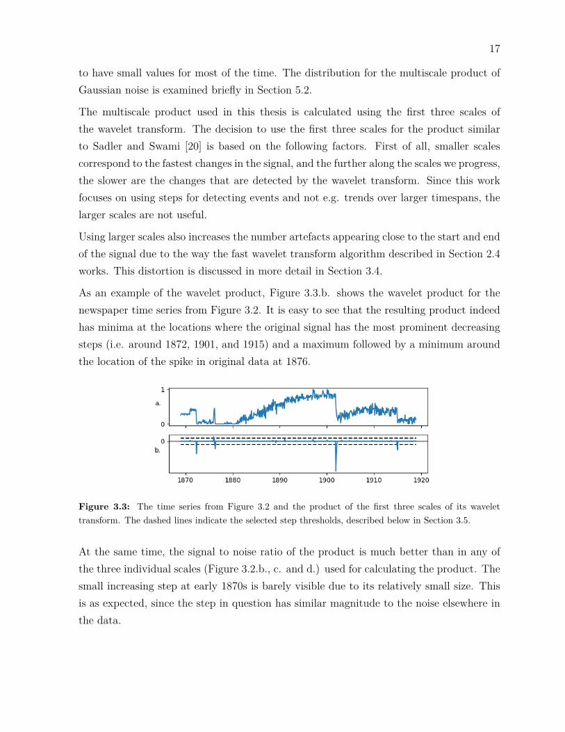
The multiscale product used in this thesis is calculated using the first three scales ofthe wavelet transform. The decision to use the first three scales for the product similarto Sadler and Swami [20] is based on the following factors. First of all, smaller scalescorrespond to the fastest changes in the signal, and the further along the scales we progress,the slower are the changes that are detected by the wavelet transform. Since this workfocuses on using steps for detecting events and not e.g. trends over larger timespans, thelarger scales are not useful.

Using larger scales also increases the number artefacts appearing close to the start and endof the signal due to the way the fast wavelet transform algorithm described in Section 2.4works. This distortion is discussed in more detail in Section 3.4.

As an example of the wavelet product, Figure 3.3.b. shows the wavelet product for thenewspaper time series from Figure 3.2. It is easy to see that the resulting product indeedhas minima at the locations where the original signal has the most prominent decreasingsteps (i.e. around 1872, 1901, and 1915) and a maximum followed by a minimum aroundthe location of the spike in original data at 1876.

Figure 3.3: The time series from Figure 3.2 and the product of the first three scales of its wavelettransform. The dashed lines indicate the selected step thresholds, described below in Section 3.5.

At the same time, the signal to noise ratio of the product is much better than in any ofthe three individual scales (Figure 3.2.b., c. and d.) used for calculating the product. Thesmall increasing step at early 1870s is barely visible due to its relatively small size. Thisis as expected, since the step in question has similar magnitude to the noise elsewhere inthe data.

18

3.4 Problems near the ends of the signal

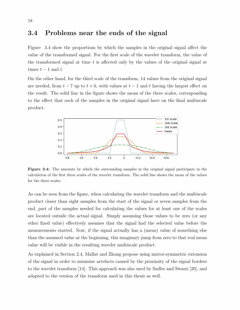
Figure 3.4 show the proportions by which the samples in the original signal affect thevalue of the transformed signal. For the first scale of the wavelet transform, the value ofthe transformed signal at time t is affected only by the values of the original signal attimes t− 1 and t.

On the other hand, for the third scale of the transform, 14 values from the original signalare needed, from t− 7 up to t+ 6, with values at t− 1 and t having the largest effect onthe result. The solid line in the figure shows the mean of the three scales, correspondingto the effect that each of the samples in the original signal have on the final multiscaleproduct.

Figure 3.4: The amounts by which the surrounding samples in the original signal participate in thecalculation of the first three scales of the wavelet transform. The solid line shows the mean of the valuesfor the three scales.

As can be seen from the figure, when calculating the wavelet transform and the multiscaleproduct closer than eight samples from the start of the signal or seven samples from theend, part of the samples needed for calculating the values for at least one of the scalesare located outside the actual signal. Simply assuming those values to be zero (or anyother fixed value) effectively assumes that the signal had the selected value before themeasurements started. Now, if the signal actually has a (mean) value of something elsethan the assumed value at the beginning, this imaginary jump from zero to that real meanvalue will be visible in the resulting wavelet multiscale product.

As explained in Section 2.4, Mallat and Zhong propose using mirror-symmetric extensionof the signal in order to minimise artefacts caused by the proximity of the signal bordersto the wavelet transform [14]. This approach was also used by Sadler and Swami [20], andadapted to the version of the transform used in this thesis as well.

19

It’s worth noting that even though the signal extension method does work in a way, thevalues for the wavelet transform and the multiscale product close to the start and end of thesignal should still be taken with a grain of salt. Figure 3.5 shows the proportion of assumeddata (i.e. values generated by the mirror extension) used for calculating each value in themultiscale product for a signal of 16 samples. For the first value (at index t = 0), theproportion of assumed data is actually more than 50 % due to the implementation detailsof the algorithm.

Figure 3.5: The proportion of assumed data used for calculating the wavelet product of a time series of16 samples

As a demonstration of the artefacts caused by the proximity of the signal borders tothe wavelet transform, Figure 3.6 shows the resulting wavelet products for signals thatcontain a single unit impulse at different locations within the signal. In Figures 3.6.a–c the minimum corresponding to the sample after the unit impulse (i.e. the decreasingstep) become increasingly exaggerated when the impulse is located near to the start ofthe signal, while the maximum disappears completely. Figure 3.6.d shows the expectedwavelet product with no interference from border effects. In Figures 3.6.e–h the maximumbecomes exaggerated while the minimum disappears.

3.5 Step detection and evaluation

After obtaining the wavelet products as described above, the products are analysed inorder to extract the step information. This process is fairly straightforward and consistsof finding local extrema in the product and interpreting them as steps. When using anodd number of scales for the wavelet product, as is done here, the maxima in the productindicate increasing steps and the minima indicate decreasing steps. If instead an evennumber of scales is used, all of the extrema corresponding to steps will be positive, and

20

Figure 3.6: Wavelet products corresponding to unit impulses at time points 0–7

the direction of each step needs to be detected e.g. based on the highest scale used in theproduct.

The main problem is in deciding the threshold that the extrema need to exceed in orderto indicate the existence of a step. In this work a relatively simple method is used: thethreshold is set to two times the standard deviation of the wavelet product being analysed.This ensures that only the extrema that exceed the signal-specific noise level are reported.

An example of the automatic thresholding can be seen in Figure 3.3.b., where the dashedlines indicate the threshold selected by the step detection. For this example, the threedecreasing steps at 1872, 1901, and 1915 exceed the threshold clearly, as does the fallingedge for the spike at 1876. The rising edge of the same spike also crosses the threshold,although not so clearly, whereas the small increase at 1871 doesn’t.

If the value of the product stays outside the threshold for more than one sample, thelocation with the highest absolute value for the product is chosen to represent the step.This means that the step is considered to happen at the point of the fastest change.

Figure 3.7 shows a closer look of the decreasing step in Dec 1901 from Figure 3.3. Similarto Figure 3.3, 3.7.a. shows the original time series and 3.7.b. shows the resulting waveletproduct, with the dashed lines showing the location of the step threshold. Here the waveletproduct is smaller than the negative threshold for three samples from Dec 1901 to Feb

21

1902. As can be seen, values further away from zero correspond to faster changes in theoriginating time series. The highest absolute value for the wavelet product occurs in Dec1901, and accordingly, that month is recorded as the time when the step occurs.

Figure 3.7: A closer look to the area around the beginning of 1902 in Figure 3.3

The location of each detected step is then stored, together with a base score which is setto the absolute value of the wavelet product at the step location divided by the thresholdvalue. This score is always ≥ 1, since the wavelet product has to be larger than thethreshold for all steps. The base scores for the steps in Figure 3.3 are listed in Table 3.1.

Step May 1872 Jan 1876 May 1876 Dec 1901 Jan 1915Score 3.86 1.44 2.42 9.27 2.73

Table 3.1: Base scores for the steps in Figure 3.3

The purpose of calculating the base score in this way is to make the steps more comparableto steps from other time series. The actual values of the wavelet product vary significantlydue to the different scales in the time series, but the score calculated in this way gives abetter idea on how distinctive the step is in its own time series.

3.6 Event detection

After obtaining a set of steps, the next step is finding events from the step information.The simplest way of doing is is by aggregating all of the steps detected per month, andusing a sum of their scores as the total score for the event. The problem with this approachis that it treats all steps equally: ten steps with a score of one will result in the same eventscore as one step with a score of ten.

Groups of a few large steps are probably more interesting than times with a larger amountof really small steps. In order to account for this, the event detection used in this thesis

22

uses only a set number of steps with the highest scores for calculating the event score.In this way, only the most significant steps for each time point affect its score, hopefullyproducing useful results.

4 Empirical evaluation

This section presents the data and experiments used for evaluating the usefulness of themethod described in Section 3. The results of the experiments are then presented inSection 5.

Section 4.1 discusses the corpus data used in latter parts of evaluating the method, andSection 4.2 describes the experiments used for evaluating the method. Section 4.2.1 dealswith the properties of the multiscale product used as part of the step detection and sec-tion 4.2.2 examines the effects of noise on step detection in a single time series. Finally,Sections 4.2.3 and 4.2.4 look into the two features found in the data that pose problemsfor event detection.

4.1 The corpus used for testing the method

The data used for testing the method consists of a collection of Finnish newspaper issuesfrom years 1869–1918. The collection contains 5352 issues of Uusi Suometar (years 1869–1918), and 2064 issues of Wiipuri (years 1893–1918). The data in the collection containsOCR data divided by page, and various metadata including the publication date.

The quality of the OCR is fairly low, and the text contains a high amount of noise,misspellings, split or combined words etc. The newspaper issues are also spread quiteunevenly within the time range, with approximately 60 percent of the issues being fromthe 15-year range 1887–1901 whereas issues from the first 15 years (1869–1883) form only9 percent of the collection.

Figure 4.1 shows for each month the percentage of days for which at least one newspaperissue exists in the data. From the figure we can see that until about halfway through 1880sthe number of newspaper issues per month stays fairly low, with especially small numberof newspaper being included in the data between 1872–1882, except for a clear spike inearly 1876. After 1882 the number of issues included in the data increases until a sharpdrop in 1901, and another in 1915. The differences in the number of issues per month aremostly due to issues missing from the dataset, instead of reflecting the actual number ofissues published.

24

Figure 4.1: Percentage of days with newspaper data in each month

Using the method for generating time series described in Section 3.1, the lemmatisationphase produced 99967 lemmas from the corpus, and discarding lemmas appearing in thecorpus less than ten times reduced the number to 48342.

Figure 4.2 is an example of a time series for a single token, in this case token suomi.Unsurprisingly, the top graph with total token counts has a similar overall shape as thegraph in Figure 4.1 showing the per-month coverage of the corpus. As for the IPM (itemsper million) values (bottom panel), having less data seems to increase the variance in theIPM values, which again is as expected due to the lower number of available samples (inthis case, newspaper issues) decreasing the reliability of the calculated mean values.

Figure 4.2: Time series of the token counts and IPM-values for the token suomi. The gaps indicatemonths for which there is no data in the corpus.

25

4.2 Testing the method

In order to evaluate the effectiveness of the method described in Section 3, various exper-iments on synthetic and real data were performed. The experiments are described below,and their results and some suggestions based on the results are presented in Section 5.

4.2.1 Properties of the multiscale product

The effectiveness of the step detection technique described in Section 3.5 was tested forvarious combinations of steps and signal to noise ratios. The purpose of these tests wasto verify that the step detection itself performs as expected, and to detect possible errorsources in this part of the method. Test time series were created with steps of varyingheight and width, and precision and recall of the step detection was measured while addingincreasing amounts of noise to the time series. The results of these tests are described inSection 5.1

Figure 4.3.a. shows the time series used to test the effect of step width to the correspondingwavelet product. Each rising step is followed by a falling step of equal height after theamount of samples defined by the step width. The step width is increased from 1 sampleto 16 samples, with the intervals between each pair of rising and falling steps set at 16samples.

Figure 4.3.b. shows the time series used to demonstrate the effect of increasing stepheights to the wavelet transform and the resulting multi-scale product. The spaces betweenthe steps and the step width were set to 10 samples to prevent interference from theneighbouring steps and the step height is increased in intervals of one. The width is basedon results from the previous test which agree with the analysis in Section 3.3 that showsthat a sample in the wavelet product at time t is affected only by samples in the originaltime series between times t− 7 and t+ 6 inclusive (see Figure 3.4).

4.2.2 The effects of noise on the step detection

First, a test signal consisting of 10000 samples of Gaussian noise (i.e. noise sampled fromthe Gaussian distribution) with variance σ2 = 1 was generated. A wavelet transformationwas performed to the signal and the wavelet product was calculated to see how the valuesof the resulting wavelet product are distributed. The first and last 10 samples of the

26

Figure 4.3: The signals used for testing the effects of step width (a.) and height (b.) to the waveletproduct.

wavelet product were discarded to remove possible interference caused by the proximityof the start and end of the signal.

Following this, precision and recall values for different combinations of signal-to-noise ratio(SNR) and step width were estimated. Precision is defined as the percentage of real stepsin all of the detected steps, and recall is the percentage of detected real steps of the totalnumber of real steps.

Precision and recall values were estimated using a test signal with five steps of equal height(see Figure 4.4). SNR was defined as

SNRdB = 10 log10A2

σ2 ,

where A is the step height and σ2 is the variance of the added noise.

Each trial consisted of the following steps. First the step height in the test signal wasadjusted to produce the desired SNR for noise with variance σ2 = 1, and the noise wasadded to the signal. Then step detection as described in Sections 3.2–3.5 was performed,and the resulting steps were compared to the known ground truth to obtain the precisionand recall values.

For each tested combination of step width (between 1–10) and SNR (-10–20dB), 5000trials were performed, which was more than enough to obtain stable results over multiple

27

Figure 4.4: The shape of the signal used in estimating the precision and recall of the step detectionusing various combinations of step width and SNR

repetitions. The results are reported in Section 5.2.

4.2.3 The effect of data coverage on the step counts

In order to get an idea on how well the step detection works using the actual corpus, thetotal numbers of steps found from the corpus was compared to step counts obtained fromsynthetic data sets spanning the same time period as the real corpus, i.e. years 1869–1918.

The synthetic data sets were generated as follows. For each month in the included timespan, n values of Gaussian noise were sampled, and the value for the month was set to themean of those n samples. Here values for n represent the number of days in each monthfor which the imaginary corpus contains data.

The first synthetic time series was generated using the same values for n that appear in thereal data. The purpose was to test whether the resulting step counts from Gaussian noisewould resemble those obtained from the actual corpus, and in what ways. The averagenumber of detected steps for each month was estimated over 10000 iterations of generatingthe data and detecting the step locations.

In addition, a second test was made using time series of steadily increasing n in orderto visualise to effect of n to the number of detected steps. Again, 10000 iterations wereperformed, and the average number of detected steps for each month was calculated. Theresults of these tests are presented in Section 5.3.

28

4.2.4 The effect of OCR errors to the step counts

When considering the effects of OCR errors to the results obtained with the describedmethod, it is useful to consider how the OCR errors affect the data. A simple wayto model OCR errors is to simply replace random characters in the original text withdifferent characters. In most cases this means that using the current system from readingthe data from the corpus, most words with replaced characters are discarded from thedata. Some changes of character simply change the word to a different valid one, butthese are probably in the minority of all changes. If we have the same probability ofchange for each of the characters in a text, longer words will have increasingly high chanceof being discarded due to one of the characters being changed.

For a single time series (corresponding to a single word), this discarding of words willsimply decrease the word counts throughout the document, assuming that the OCR errorrate is similar throughout the corpus. This decrease will decrease the signal-to-noise ratiofor that word, with results similar to those of increasing the noise level, discussed inSection 5.2. If there is a sharp change in the OCR quality, for instance caused by a changein the typeface used in the newspaper, this should result in steps being detected for a largenumber of words at the same time point, assuming that the change in quality is significantenough.

Since the effects of OCR error should be effectively the same as examined with the earliertests, no separate tests for analysing these effects were performed.

5 Results

5.1 Properties of the multiscale product

Figure 5.1 shows the effect of step width to the amplitude of spikes in the resulting waveletproduct. The signal used for testing is depicted in Figure 5.1.a. and the resulting waveletproduct is presented in Figure 5.1.b. The width of each of the steps has been markedbelow 5.1.b. for improved legibility.

As can be seen from the figure, the spike heights in the wavelet product increase withthe step width until steps of width seven, after which the step width doesn’t affect themagnitude of the spike. The lower heights for small step widths are cause by destructive in-terference between the neighbouring rising and falling steps. In the remaining experiments,ten samples is used as a sufficient distance between steps in order to avoid interferencefrom neighbouring steps.

Figure 5.1: Growth of the wavelet product for increasing step width.

Figure 5.2 shows a sequence of steps with increasing heights (a.) and the correspondingwavelet product (b.). The widths of the steps and the intervals between them have beenset to 10 samples based on the results of the previous test. This distance between separate

30

steps is enough to prevent interference from neighbouring steps. The values of the waveletproduct show cubic growth, which is expected: each scale of the wavelet transform shouldscale linearly in proportion to the original signal, and the wavelet product is the productof three scales of the transform, resulting in cubic growth in relation to the step height,other parameters being constant.

Figure 5.2: Growth of the wavelet product for increasing step height.

5.2 The effects of noise on the step detection

Figure 5.3 shows the distribution of values in the wavelet product for signal consisting ofGaussian noise with zero mean and standard deviation σ = 1. The figure is essentially areproduction of a similar figure presented by Sadler and Swami [20]. Standard deviationof the wavelet product is approximately 3.2, and the black lines in the image show thevalues of 2σ used as the threshold for step detection. Approximately 4.4% of the samplesin the wavelet product fall outside of the thresholds resulting in false positive steps. Anormal distribution with the same standard deviation of 3.2 is also drawn to the imagefor comparison.

Figure 5.4 shows the effect of step width on the precision of step detection for differentsignal-to-noise ratios. For most of the step widths, the precision levels are pretty closeregardless of SNR, with higher step widths obtaining slightly better results throughout.

31

Figure 5.3: A histogram of the wavelet product values for Gaussian noise.

Precision for step widths of one and two is clearly worse from the others. For step widthtwo being approximately 0.1 lower than the main group between SNRs 2–12 dB, and forstep width of one (i.e. spikes in the signal) the precision is approximately 0.4 below themain group around SNR of 10dB.

Figure 5.4: Precision for different step widths with varying SNR.

Figure 5.5 shows the estimated recall values for the step detection for various step widthsand SNRs. Compared to the precision values, the recall values for different step widthsare more spread, with distance between the steps approximately halving for each increasein step width. In terms of recall, the spikes do quite badly, staying under 0.5 even forSNR of 20 dB.

The poor recall results for the spikes and narrow steps are likely due to the fact that therising and falling edges interfere with each other quite strongly, causing one of the two

32

Figure 5.5: Recall for different step widths with varying SNR.

to stay undetected. Figure 5.6 shows recall values when detecting either edge of the stepis counted as detecting the whole step. In this case, recall levels similar to the ones inFigure 5.5 for SNR of 20dB are reached already at around 13dB. Especially the narroweststeps are detected significantly better when making this allowance.

Figure 5.6: Recall for different step widths with varying SNR when detecting either edge of the step iscounted as detecting the entire step.

5.3 The effect of data coverage on the step counts

As mentioned earlier in Section 4.1, the coverage of the included time span in the corpusis quite uneven. For some months, only a few days worth of newspapers are included inthe corpus while for others, the number goes up to thirty.

33

In order to investigate the effect of the amount of available data on the step counts, thefirst test was to perform step detection for each of the words in the actual corpus, andcount the the total number of steps detected for each month in the data. Figure 5.7 showsthe number of steps detected in the corpus for each month.

Figure 5.7: The number of steps per month detected by the step detection

As can be seen from comparison to Figure 5.8, repeated here from page 24 for convenience,the number of detected steps seems to have a strong inverse correlation with the amountof data available for the month in question, with less data producing more steps. Thismakes sense since the monthly IPM values are essentially estimated means for the dailyIPM values, and having less data points available would naturally make the estimates lessaccurate, and increase their variance, which results in large number of false positives.

Figure 5.8: Percentage of days with newspaper data in each month, repeated from page 24 for conve-nience

Figures 5.9 and 5.10 show average step counts per month for two different synthetic datasets. Figure 5.9 shows the result when sampling Gaussian noise instead of values in thecorpus, but using the same amount of samples per month as the real corpus contains.

It is easy to see that the overall shapes of Figures 5.7 and 5.9 are quite similar. One of themost clear differences between the graphs seem to be the spike in January 1874, which ismissing from the real data, likely due to some difference in the way how months with no

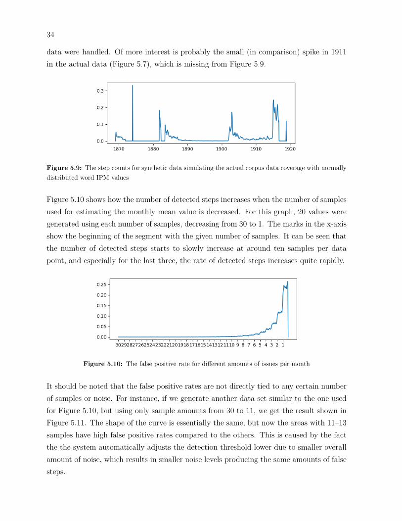
34

data were handled. Of more interest is probably the small (in comparison) spike in 1911in the actual data (Figure 5.7), which is missing from Figure 5.9.

Figure 5.9: The step counts for synthetic data simulating the actual corpus data coverage with normallydistributed word IPM values

Figure 5.10 shows how the number of detected steps increases when the number of samplesused for estimating the monthly mean value is decreased. For this graph, 20 values weregenerated using each number of samples, decreasing from 30 to 1. The marks in the x-axisshow the beginning of the segment with the given number of samples. It can be seen thatthe number of detected steps starts to slowly increase at around ten samples per datapoint, and especially for the last three, the rate of detected steps increases quite rapidly.

Figure 5.10: The false positive rate for different amounts of issues per month

It should be noted that the false positive rates are not directly tied to any certain numberof samples or noise. For instance, if we generate another data set similar to the one usedfor Figure 5.10, but using only sample amounts from 30 to 11, we get the result shown inFigure 5.11. The shape of the curve is essentially the same, but now the areas with 11–13samples have high false positive rates compared to the others. This is caused by the factthe the system automatically adjusts the detection threshold lower due to smaller overallamount of noise, which results in smaller noise levels producing the same amounts of falsesteps.

35

Figure 5.11: The false positive rate for different amounts of issues per month, with higher overall numberof available data

5.4 Performance of the event detection

Finally, the event detection was performed on the real corpus, and the resulting events andtheir scores were examined in more detail. Figure 5.12 show the event scores described inSection 3.6 for all points on the time series. The scores were calculated using four differentvalues for the number of steps to be included in calculating the score.

Figure 5.12: The event scores for different time points, using a. 5, b. 10, c. 20, and d. 50 highestscoring steps for calculating the event score

In all of the graphs, the overall shape of the graph is quite similar to the one in Fig-ure 5.9 showing that the event detection is affected significantly by the effects describedin Section 5.3.

6 Discussion

6.1 Effects of noise and missing data on the system

Based on the results, wavelet analysis seems to be a reasonable choice for step detection,especially when it can be assumed that the steps are wider than one or two samples. Forspikes, detection of both rising and falling edges in quite poor, resulting often in only oneof the two being detected. This is visible in Figure 5.5, where the recall for width of oneis fairly poor. In order to classify spikes correctly, some additional analysis mechanismsshould probably be employed after finding the step locations using the step detectionmethod described in this work.

Another feature of the step detection examined in this work is the automatic scalingemployed in deciding the detection threshold for steps. Selecting the threshold valuebased on the standard deviation in the multiscale product works reasonably well when thenoise level in the data is fairly constant. When using the threshold value of two timesthe standard deviation, as was done in this thesis, the rate of false positives for a signalconsisting of Gaussian noise is around 4.4 % (see Section 5.2). Any actual steps in thedata increase the standard deviation, resulting in reduced false positive rate.

On the other hand, if the noise level is not constant, the parts of the signal with less noisecause the detection threshold to become smaller, resulting in increased amount of falsepositives in the more noisy parts. This is demonstrated in Figures 5.10 and 5.11, wherecutting the noisiest parts of the data in Figure 5.10 (the areas with 1–10 samples) simplydrops the detection threshold and results in the curve in Figure 5.11 with a really similaroverall shape.

OCR errors in the data have similar effects to noise, and as can be seen from Figures 5.4and 5.5, will cause a decrease in the precision and recall properties of the step detection.Especially the recall for spikes and narrow steps in the data is quite poor in the presenceof noise, and OCR noise will therefore reduce the system’s ability to detect them.

37

6.2 Alleviating the effects of uneven temporal distri-bution of data

Uneven distribution of the data in the corpus causes significant distortion in the detectedsteps, and needs to be addressed in order to improve the reliability of the system. Twoways of doing this were considered, each with their own downsides.

The first way is to add weights to the scores (see Section 3.5) calculated for each stepbased on the amount of data available at that time point. Smaller amounts of data meanthat the detected steps are less reliable, and therefore should be given less weight whencomparing to other steps.

However, selecting the weights in a useful way is not trivial, because the difference inreliability between different amounts of available data depends on the overall levels ofavailable data in the time series, as demonstrated in Figures 5.10 and 5.11. When thesmallest amount of monthly issues in the time series is 11, the false positive rate formonths with 11 issues is over 20% (figure 5.11, whereas for another set of data where somemonths have only single issues, the false positive rate for 11 issues per month is around1%.

The second, easier way is to change the way the time series are formed. Since the numberof samples used per data point is the key factor in adjusting the noise level, it should bepossible to generate the time series by forming even sized groups of samples that mightspan different amounts of time. In this way, it should be possible to avoid the varyingnoise levels caused by different number of samples.

On the other hand, for time periods with less available data, this would result in poorertime resolution, since a single group would contain the data from a longer time period.Also, since the time intervals would be longer, this might mean that the changes happeningin those periods would seem faster and therefore more interesting than they should. Still,this seems like a solution that should be experimented on in order to measure its usefulness.

Yet another method that would be an interesting subject of further research would beto look for ways to adjust the step threshold locally instead of having a single thresholdfor the whole time series. A simple example would be to calculate the step thresholdseparately for each time point, using only the n closest values of the multiscale product,with some large enough value for n.

38

6.3 Problematic features of the method, and sugges-tions for improvements

One of the problems detected during the testing of the system is that the signal extensionat the start and beginning of the signal may cause significant artefacts in the analysis (seeSection 3.4). Combined with the the way the step threshold is selected for each time seriesthese artefacts can basically ruin the whole time series. As shown in Figure 3.1, even asmall spike caused by noise can be significantly exaggerated if it happens to be located inthe first sample of the time series. By itself this simply means that there will be a falsepositive falling edge in the analysis results, and this could be fixed by simply ignoring allsteps detected within five or so samples of the start and end of the signal.

However, since the proximity of the signal border causes the spike to seem ten times itsreal size, it will also cause the step threshold to increase, potentially causing any real stepsin the data to go unnoticed. Simply ignoring the step results close to the borders will notcorrect this problem. A simple fix would be to ignore the same samples in the multiscaleproduct also when deciding the step threshold. In other words, instead of calculatingthe standard deviation of the whole multiscale product, the standard deviation would becalculated only using the parts of the product not affected by the artefacts, i.e. everythingexcept the first seven and the last six samples.

Another related problem in the implementation is how the mirror extension is imple-mented. Currently the mirror extension is performed separately at the start of every loopin the algorithm, and the resulting signals are then trimmed back to the original size.This means that for calculating the first three scales of the wavelet transform, the mirrorextension if performed not once but three times, each time distorting the original signal.

Instead, it the algorithm should be modified so that it would perform the extension just atthe beginning, and then use the extended signal without trimming it back down at everyrepetition. This should at least slightly reduce the artefacts close to the signal borders,even though removing them completely is not possible. Unfortunately this improvementwasn’t added to the system due to time constraints, but it should be an easy modificationfor further research projects.

39

6.4 Conclusions

Although the step detection works reasonably well even in a noisy environment for stepswider than a few samples, its applicability on event detection remains uncertain. Addi-tional research is needed to find ways of reducing the impact of features in the data suchas the uneven temporal distribution and the high amount of noise. Improving the qualityof the used data is one way to improve the situation, and could lead to improved qualityof the detected steps and the related events. Some minor improvements unrelated to theissues with the data were also suggested, but by themselves they aren’t likely to improvethe overall quality of the event detection significantly.

Bibliography

[1] F. Atefeh and W. Khreich. “A survey of techniques for event detection in twitter”.In: Computational Intelligence 31.1 (2015), pp. 132–164. doi: 10.1111/coin.12017.

[2] S. G. Chang, B. Yu, and M. Vetterli. “Adaptive wavelet thresholding for imagedenoising and compression”. In: IEEE transactions on image processing 9.9 (2000),pp. 1532–1546. issn: 1941-0042. doi: 10.1109/83.862633.

[3] S.-W. Chen, H.-C. Chen, and H.-L. Chan. “A real-time QRS detection methodbased on moving-averaging incorporating with wavelet denoising”. In: Computermethods and programs in biomedicine 82.3 (2006), pp. 187–195. issn: 0169-2607.doi: 10.1016/j.cmpb.2005.11.012.

[4] I. Daubechies. Ten lectures on wavelets. Vol. 61. CBMS-NSF Regional ConferenceSeries in Applied Mathematics. SIAM, 1992. isbn: 9781611970104.

[5] A. Grossmann and J. Morlet. “Decomposition of Hardy functions into square inte-grable wavelets of constant shape”. In: SIAM journal on mathematical analysis 15.4(1984), pp. 723–736. doi: 10.1137/0515056.

[6] M. Hamalainen. “UralicNLP: An NLP Library for Uralic Languages”. English. In:Journal of open source software 4.37 (2019). issn: 2475-9066. doi: 10.21105/joss.

01345.

[7] W. He, Y. Zi, B. Chen, F. Wu, and Z. He. “Automatic fault feature extractionof mechanical anomaly on induction motor bearing using ensemble super-wavelettransform”. In: Mechanical Systems and Signal Processing 54-55 (2015), pp. 457–480. issn: 0888-3270. doi: 10.1016/j.ymssp.2014.09.007.

[8] A. Liu. “The state of the digital humanities: A report and a critique”. In: Arts andHumanities in Higher Education 11.1-2 (2012), pp. 8–41. doi: 10.1177/1474022211427364.

[9] E. Loper and S. Bird. “NLTK: the natural language toolkit”. In: arXiv preprintcs/0205028 (2002).

[10] S. M. LoPresto, K. Ramchandran, and M. T. Orchard. “Image coding based on mix-ture modeling of wavelet coefficients and a fast estimation-quantization framework”.In: Proceedings DCC’97. Data Compression Conference. IEEE. 1997, pp. 221–230.doi: 10.1109/DCC.1997.582045.

42 BIBLIOGRAPHY

[11] T. Lotze, G. Shmueli, S. Murphy, H. Burkom, et al. “A wavelet-based anomalydetector for early detection of disease outbreaks”. In: Workshop on Machine LearningAlgorithms for Surveillance and Event Detection, 23rd Intl Conference on MachineLearning. International Conference on Machine Learning. 2006.

[12] W. Lu and A. A. Ghorbani. “Network anomaly detection based on wavelet analysis”.In: EURASIP Journal on Advances in Signal Processing 2009 (2009), p. 4. issn:1110-8657. doi: 10.1155/2009/837601.

[13] S. Mallat and W. L. Hwang. “Singularity detection and processing with wavelets”.In: IEEE transactions on information theory 38.2 (1992), pp. 617–643. issn: 1557-9654. doi: 10.1109/18.119727.

[14] S. Mallat and S. Zhong. “Characterization of signals from multiscale edges”. In: IEEETransactions on Pattern Analysis & Machine Intelligence 14.7 (1992), pp. 710–732.issn: 1939-3539. doi: 10.1109/34.142909.

[15] NewsEye. What is NewsEye about?, accessed 14.10.2019. url: https : / / www .

newseye.eu/about/.

[16] A. Noiboar and I. Cohen. “Anomaly detection based on wavelet domain GARCHrandom field modeling”. In: IEEE transactions on geoscience and remote sensing45.5 (2007), pp. 1361–1373. issn: 1558-0644. doi: 10.1109/TGRS.2007.893741.

[17] S. Petrovic, M. Osborne, and V. Lavrenko. “Streaming first story detection with ap-plication to twitter”. In: Human language technologies: The 2010 annual conferenceof the north american chapter of the association for computational linguistics. HLT’10. Association for Computational Linguistics. 2010, pp. 181–189. isbn: 1-932432-65-5.

[18] S. Phuvipadawat and T. Murata. “Breaking news detection and tracking in Twit-ter”. In: 2010 IEEE/WIC/ACM International Conference on Web Intelligence andIntelligent Agent Technology. Vol. 3. IEEE. 2010, pp. 120–123. doi: 10.1109/WI-

IAT.2010.205.

[19] A. Rosenfeld. “A nonlinear edge detection technique”. In: Proceedings of the IEEE58.5 (1970), pp. 814–816. issn: 1558-2256. doi: 10.1109/PROC.1970.7756.

[20] B. M. Sadler and A. Swami. “Analysis of multiscale products for step detection andestimation”. In: IEEE Transactions on Information Theory 45.3 (1999), pp. 1043–1051. issn: 1557-9654. doi: 10.1109/18.761341.

BIBLIOGRAPHY 43

[21] O. Sayadi and M. B. Shamsollahi. “Multiadaptive bionic wavelet transform: Appli-cation to ECG denoising and baseline wandering reduction”. In: EURASIP Journalon Advances in Signal Processing 2007.1 (2007). issn: 1687-6180. doi: 10.1155/

2007/41274.

[22] P. Svensson. “Humanities computing as digital humanities”. In: Defining DigitalHumanities. Routledge, 2016, pp. 175–202. doi: 10.4324/9781315576251.

[23] D. Taubman and M. Marcellin. JPEG2000 image compression fundamentals, stan-dards and practice: image compression fundamentals, standards and practice. Vol. 642.The Springer International Series in Engineering and Computer Science. SpringerScience & Business Media, 2012. isbn: 9781461507994.

[24] T. Van Canh, K. Markert, and W. Nejdl. “A Framework For Historical RussianFlu Epidemic Exploration From German Newspapers.” In: Digital Humanities 2017Conference Abstracts (2017), pp. 630–633.

[25] R. W. White and R. A. Roth. “Exploratory search: Beyond the query-responseparadigm”. In: Synthesis lectures on information concepts, retrieval, and services1.1 (2009), pp. 1–98. doi: 10.2200/S00174ED1V01Y200901ICR003.

[26] Y. Xu, J. B. Weaver, D. M. Healy, and J. Lu. “Wavelet transform domain filters: aspatially selective noise filtration technique”. In: IEEE transactions on image pro-cessing 3.6 (1994), pp. 747–758. issn: 1941-0042. doi: 10.1109/83.336245.