A measure of spatial disorder

in particle methods

M. Antuono a, B. Bouscasse a, A. Colagrossi a,∗, S. Marrone a,b

aCNR-INSEAN, Marine Technology Research Institute, Rome, ItalybÉcole Centrale Nantes, LHEEA Lab. (UMR CNRS), Nantes - France

Abstract

In the present work we describe a numerical algorithm which gives a measure ofthe disorder in particle distributions in two and three dimensions. This applies toparticle methods in general, disregarding the fact they use topological connectionsbetween particles or not. The proposed measure of particle disorder is tested onspeci�c con�gurations obtained through perturbation of a regular lattice. It turnsout that the disorder measure may be qualitatively related to the mean absolutevalue of the perturbation. Finally, some applications of the proposed algorithm areshown by using the Smoothed Particle Hydrodynamics (SPH) method.

Key words: Particle Methods, Meshless Methods, Particle Disorder, SmoothedParticle Hydrodynamics

1 Introduction

In recent years a large amount of studies on particle methods have beendeveloped, these concerning several �elds of Physics, Engineering andMathematics. The increasing interest in particle methods has been driven bytheir powerful applications and by the attractive mathematical backgroundon which they rely. The main advantage of particle schemes is that they donot implement �xed computational grids but use particles as computationalnodes and move them in a Lagrangian fashion. This allows the modeling ofcomplex dynamics with large deformations of the computational domain.

∗ Corresponding author: Tel.: +39 06 50 299 343; Fax: +39 06 50 70 619.Email addresses: matteo.antuono@cnr.it (M. Antuono),

benjamin.bouscasse@cnr.it (B. Bouscasse), andrea.colagrossi@cnr.it (A.Colagrossi), salvatore.marrone@cnr.it (S. Marrone).

Preprint submitted to Elsevier Science 11 May 2015

Generally, these schemes may be divided in two wide classes: those which usetopological connections between particles (i.e. [1]) and meshless methods (like,for example, [2,3]). For all these schemes, the attainment and maintenanceof a regular particle distribution is a crucial point, since the particledisorder may strongly a�ect their accuracy and stability [4,5]. This challengedmany researchers to regularize the particle arrangement through remeshingor shifting algorithms (see, for example, [6�8]). Notwithstanding the ideaof particle order/disorder is a natural and innate concept, its theoreticalde�nition and quantitative measurement is hard to identify in a clear andunambiguous manner. This is what we try to address in the present work: wepropose a measure of the particle disorder and check it on a number of testcases. These have been gathered in two groups: the former one is made byapplications of the disorder measure on di�erent particle distributions whilethe latter one contains dynamical test cases obtained by using a SmoothedParticle Hydrodynamics (SPH) scheme.

The basic idea for the particle disorder measure relies on the de�nitionof two di�erent local distances (that is, distances related to each singleparticle). The �rst local distance is simply the minimum distance of a particlefrom its neighbor particles. The de�nition of the second local distance ismore complex, since this must account for any directional anisotropy in theparticle distribution. This may be computed by searching the nearest neighborparticles in di�erent directions and, then, taking the maximum distance allover them.

By construction, the second distance is greater or equal to the �rst distance.Hence, we de�ne a local disorder measure as the ratio between half thedi�erence between the second and the �rst distance and their arithmetic mean.A global disorder measure is obtained as the arithmetic mean of the localmeasure all over the particles. If the distribution is regular, the �rst and seconddistances coincide all over the computational domain, the local measure is zeroeverywhere and so does the global measure (see Section �2). Then, intuitively,the global measure represents how far the actual particle distribution is froma regular lattice. In Section �2.1 we heuristically found that it has the sameorder of magnitude of the mean absolute error of the particle distributionwith respect to an hypothetical regular distribution. Finally, in Section �3 theglobal measure has been applied to study dynamical test cases.

2 The particle disorder measure

Let us consider a particle i at the position ri. In particle methods, the i-th particle has its own neighbor particles which may be identi�ed throughtopological connections (e.g. PFEM) or as particles inside a proper domain

2

Nii θ

v̂

Ci(v̂)

Fig. 1. Sketch of a generic set of the neighbor particles, Ni (green shaded area), andof the cone Ci(v̂) with angle 2 θ and axis direction v̂ (red shaded area). The selectedparticle is the nearest to the i-th particle inside the cone.

(as, for example, the compact support of the kernel function in SPH). Wedenote the set of the neighbor particles to the particle i as Ni (note that Ni

does not include the i-th particle itself). We de�ne the �rst local distance asfollows:

d (i)m = min

j∈Ni

‖rj − ri‖ , (1)

where rj is the position of the j-th neighbor particle. If Ni is empty, d (i)m is

set equal to zero. This is an arbitrary choice and it means that we considerisolated/not-connected particles as a part of disconnected computationaldomains.

To construct the second local measure, we �rst de�ne the right circular cone.The vertex of the cone is placed on the i-th particle and its axis is identi�edby a unit vector v̂. The cone aperture is denoted through 2θ. Then, the coneis given by:

Ci(v̂)=

{r ∈ Rd such that

(r − ri)‖r − ri‖

· v̂ ≥ cos(θ)

}, (2)

where d indicates the spatial dimension. A sketch of the cone is displayed in�gure 1. The de�nition of the angle θ is of crucial importance. Speci�cally,we require that, in the presence of a regular lattice, the cone includes at leastone of the nearest neighbor particles (see �gure 2). In two dimensions onlythree regular distributions are possible, namely, the Triangular, the Cartesianand the Hexagonal one. Among these, the Hexagonal distribution has thelargest angle between two subsequent nearest particles, i.e. 2π/3 radiants.This suggests that θ has to be larger than π/3. In three dimensions, the onlyregular lattice is the Cartesian grid. In this case, we require the cone to be

3

Fig. 2. a sketch with the Cartesian tessellation. Left: a cone with large enough valueof θ. Right: a cone with a wrong value of θ.

large enough to include an octant. This corresponds to cos(θ) > 1/√

3 which,similarly to the two dimensional case, approximately corresponds to choosingθ ≥ π/3. The in�uence of θ on the results is analyzed in Section �2.1. In allthe cases, the axis direction v̂ is arbitrary.

After the cone has been de�ned, we select the neighbor particles inside itand compute the minimum distance from the i-th particle. Then, the coneis rotated (this corresponds to a rotation of the axis or, equivalently, of thevector v̂) and the procedure is repeated. In numerical simulations it is notpossible to rotate the cone continuously. For this reason, we select a �nitenumber of rotations to obtain a cover of the neighborhood of the particle i.This strategy in�uences the value of the measure we are going to de�ne but itdoes not alter its global properties. This aspect will be examined in-depth inSection �2.1. For the time being, let us assume that there are k rotations of thecone or, equivalently, k cones with axes identi�ed by unit vectors v̂k. Whenthe neighborhood of the i-th particle has been covered, the second distance isset equal to the supremum of the minimum distances, that is:

d(i)M = max

k

{min

j∈Ni|rj∈Ci(v̂k)‖rj − ri‖

}. (3)

A sketch of the procedure is drawn in �gure 3. By construction, this de�nitionallows detecting any eventual anisotropy in the particle distribution and, incase of a regular lattice, it coincides with d (i)

m . If any of the k cones is empty(that is, no neighbor particles are inside it), the minimum distance inside itis set equal to zero. This is done to be consistent with the case in which theparticle i has no neighbor particle at all. In this way, the above de�nitionsimply d

(i)M = d (i)

m = 0.

By construction, the second distance is greater or equal to the �rst distance.Hence, we de�ne a local disorder measure as follows:

4

Fig. 3. a sketch of the procedure to build the second distance, d(i)M . Left: the selected

particle is the nearest inside the cone. Right: the colored particles are the nearest in

each cone. The farthest among them gives d(i)M .

λi =

d(i)M − d (i)

m

d(i)M + d

(i)m

if d(i)M > 0 ,

0 if d(i)M = 0 .

(4)

The latter case corresponds to isolated particles. Obviously, we exclude fromthe present analysis the eventuality that all (or a great part of) the particlesare isolated. Finally, the global measure of the particle disorder is de�ned asfollows:

Λ =

∑i λiN

, (5)

where the summation is performed over all particles and N is the total numberof particles. Since λi ≤ 1, it is Λ ≤ 1 as well. If the particle distribution isregular, the second and �rst local distances coincide all over the computationaldomain. Consequently, λi is zero everywhere and Λ = 0. This means that wecan use Λ as a qualitative measure which indicates how far the actual particledistribution is from a regular lattice. In the next section, we show that Λhas the same order of magnitude of the mean absolute error of the particledistribution with respect to an hypothetical regular distribution.

Before proceeding to the analysis, we would like to stress a further point. Nohypothesis has been done on the set of neighbor particles, meaning that themeasure Λ is well posed whatever the form of Ni. Speci�cally, the de�nitionof Ni only depends on the numerical scheme under consideration.

5

2.1 Tests on irregular particle distributions

In this section we use Λ to measure the disorder on irregular particledistributions. These have been obtained by superimposing a random noise(Gaussian or Uniform) on regular distributions (Hexagonal, Cartesian andTriangular in two dimensions and Cartesian in three dimensions) characterizedby a mean particle distance equal to ∆x. The random noise has zero meanand mean absolute value equal to εr ∆x. Speci�cally:

εr =1

N

∑i

‖ri − r̂i‖∆x

, (6)

where r̂i indicates the particle position on the regular grid. This parameterrepresents the mean absolute relative error with respect to the regular grid. Asshown in the sequel, εr can be easily correlated with the measure of disorderand, therefore, it is preferred to a characterization based on the variance ofthe random noise (as done, for example, in Vacondio et al. [9]). Incidentally,we observe that the variance is not constant but depends on εr because of theassignment on this parameter. This is explained in details in appendix A. Theresults shown in the sequel have been obtained by using a squared domainwith about 6400 particles (the number of particles slightly varies according tothe tessellation under consideration).

The analysis of the measure Λ is made by varying the angle θ and the numberof cones (see Section �2). As explained in the previous section, the directionsof the cone axes are completely arbitrary since we just need to cover theneighborhood of the i-th particle. In any case, we prefer to give a recipe to setthese directions in a simple and reliable way. Let us consider k cones centeredon the i-th particle. The axis of the �rst cone is de�ned by using the directiongiven by the i-th particle and its closest neighbor particle. In two dimensionsthe remaining (k − 1) directions are selected by dividing the two-dimensionalspace in k identical sectors. For what concerns the three dimensional space,the possibility of choosing the remaining directions in a �regular� way islimited to few speci�c cases. For example, the axis directions may be chosenas the vertexes of regular polyhedra centered on the i-th particle. This leadsto k = 4, 6, 8, 12, 20 according to the adopted polyhedron (e.g., tetrahedron,octahedron, cube, icosahedron or dodecahedron).

The �rst three plots of �gure 4 display the behavior of the measure Λ appliedto two-dimensional regular grids perturbed by a Gaussian noise (εr = 0.1). Theerror bars represent the variance of the local measure λi. We vary both thenumber of cones and the angle θ. In all the cases the increase of the number ofcones generally corresponds to a slight increase of Λ even if the discrepanciesrapidly decrease as the angle becomes larger and larger. Speci�cally, for values

6

Fig. 4. The measure Λ applied to two-dimensional regular grids and to a Cartesianthree dimensional grid perturbed by a Gaussian noise (εr = 0.1). The angle θ ismeasured in degrees.

of θ that are su�ciently large, the measure Λ seems to approach a plateau.This �asymptotic� value of Λ has an order of magnitude which is comparableto the error εr (plotted as the abscissa) and this means that Λ may beused as a qualitative measure for the particle disorder. Similar behavior hasbeen observed in three dimensions (see the bottom right panel of �gure 4).These results maintain almost identical by using a Uniform noise instead of aGaussian noise. Incidentally, we recall that Λ is well posed only for θ > π/3(see previous section) and this motivates the large discrepancies observed in�gure 4 when θ < π/3.

The above analysis suggests that it is not necessary to use a large numberof cones but it is preferable (and computationally more convenient) to usefew cones with a large enough angle. Then, in both two and three dimensionswe choose 8 cones and θ = 7π/18 (that is, θ = 70◦). Some examples of thebehavior of the measure Λ with θ = 7π/18 are drawn in �gure 5 as functionof the noise εr. These plots con�rm that Λ is comparable to εr and that themeasure is only slightly in�uenced by the increase of the number of cones.

7

Fig. 5. The measure Λ with θ = 70◦ applied to two-dimensional regular grids and toa Cartesian three dimensional grid perturbed by a Gaussian noise.

3 Applications

In the following sections we show some useful applications of the proposedmeasure of spatial disorder. We use the Smoothed Particle Hydrodynamicsscheme (SPH hereinafter) since this is one of the most widespread particlemethods in the �uid-dynamics community. In its standard form, the SPHscheme relies on the assumption that the �uid is weakly-compressible andbarotropic. Speci�cally, the SPH equations read:

8

DρiDt

= − ρi∑j

(uj − ui) · ∇iWij Vj

Dui

Dt= − 1

ρi

∑j

(pj + pi)∇iWij Vj + f i +µ

ρi

∑j

πij∇iWij Vj

DriDt

= ui pi = c20 ( ρi − ρ0 )

(7)

where ρi, Vi, pi are respectively the density, the volume and the pressure of thei−particle while ri and ui are its position and velocity. Here, Wij is a weightfunction (also known as kernel function) which accounts for the interactionswith the neighbor particles. The kernel function depends on ‖rj − ri‖ andhas a compact support which automatically de�nes the set Ni. The radius ofthe compact support is proportional to a reference length, h, which is calledsmoothing length. Speci�cally, we choose a Wendland kernel with a supportradius equal to 2h = 4 ∆x. The symbol ∇i denotes the di�erentiation withrespect to ri and f i is the body force at the position ri. Finally, symbols ρ0 andc0 indicate the reference density and sound velocity (assumed to be constant).For computational reason, it is common practice in the weakly-compressibleSPH solvers not to use the physical sound velocity but, conversely, to impose c0to be at least one order of magnitude greater than the maximum �ow velocity,that is, c0 ≥ 10 maxi ‖ui‖. This assumption ensures the density variation toremain below 1%.

The viscous e�ects are modeled through the formulation proposed byMonaghan and Gingold [10]. The dynamic viscosity is denoted through µwhile the kinematic viscosity is ν = µ/ρ0. The argument of the viscous termis:

πij = K(uj − ui) · (rj − ri)

‖rj − ri‖2, (8)

where K = 2 (n + 2) and n is the number of spatial dimensions. Underthe assumption that the �uid is incompressible, this term approximates theLaplacian of the velocity �eld (see, for example, [11]). For what concerns thetime step, this is chosen as the minimum over three di�erent reference timeswhich represent the viscous, the advective and the acoustic time scales. Theseare respectively:

9

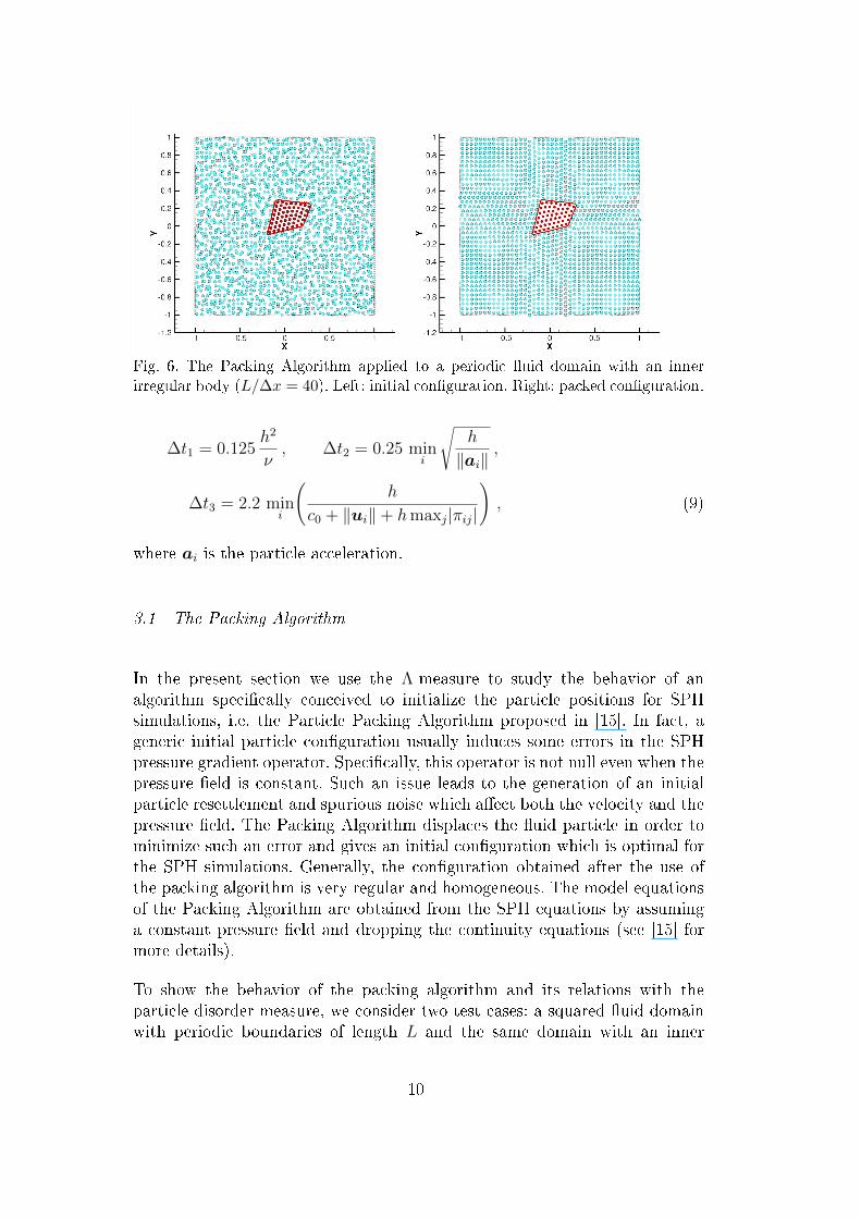
Fig. 6. The Packing Algorithm applied to a periodic �uid domain with an innerirregular body (L/∆x = 40). Left: initial con�guration. Right: packed con�guration.

∆t1 = 0.125h2

ν, ∆t2 = 0.25 min

i

√h

‖ai‖,

∆t3 = 2.2 mini

(h

c0 + ‖ui‖+ hmaxj|πij|

), (9)

where ai is the particle acceleration.

3.1 The Packing Algorithm

In the present section we use the Λ-measure to study the behavior of analgorithm speci�cally conceived to initialize the particle positions for SPHsimulations, i.e. the Particle Packing Algorithm proposed in [15]. In fact, ageneric initial particle con�guration usually induces some errors in the SPHpressure gradient operator. Speci�cally, this operator is not null even when thepressure �eld is constant. Such an issue leads to the generation of an initialparticle resettlement and spurious noise which a�ect both the velocity and thepressure �eld. The Packing Algorithm displaces the �uid particle in order tominimize such an error and gives an initial con�guration which is optimal forthe SPH simulations. Generally, the con�guration obtained after the use ofthe packing algorithm is very regular and homogeneous. The model equationsof the Packing Algorithm are obtained from the SPH equations by assuminga constant pressure �eld and dropping the continuity equations (see [15] formore details).

To show the behavior of the packing algorithm and its relations with theparticle disorder measure, we consider two test cases: a squared �uid domainwith periodic boundaries of length L and the same domain with an inner

10

Fig. 7. The Packing Algorithm with and without the solid body for L/∆x = 40.Top panel: evolution of Λ. Bottom panel: error on the pressure gradient. Here, p0 isthe reference pressure �eld and h is the reference length for the kernel support(alsoknown as smoothing length). The ordinate axis shows the number of iterations ofthe Packing Algorithm.

irregular solid body (see �gure 6). In both the cases, the particles are initiallyset on a Cartesian grid perturbed by a random noise (εr = 0.25, see Section2.1) and the packing algorithm is used to attain a stable con�guration. Asexpected, in the �rst case we obtain a regular con�guration (speci�cally, weobtain back a Cartesian grid). Conversely, the presence of the solid body leadsto a �nal con�guration which is not perfectly regular (see the right panel of�gure 6) even if it is characterized by a small value of Λ. This is shown in�gure 7 where the evolution of Λ is displayed along with the L2-error onthe pressure gradient operator. In both the cases the error rapidly convergesto zero, ensuring that the �nal particle con�guration is stable (that is, it isnot a�ected by a further particle resettlement). Conversely, the evolution ofdisorder measure is quite di�erent. In fact, the presence of the solid bodyimplies that Λ does not converge to zero, even though its asymptotic value isquite small (Λ ' 10−2). This is an important point since it means that theSPH admits stable particle con�gurations even though such con�gurations arenot perfectly regular.

3.2 Disorder and SPH Interpolation

Before proceeding to the analysis, it is interesting to draw some connectionsbetween the particle disorder and the SPH interpolation.

11

All SPH schemes rely on a smoothing procedure that, at the continuum,allows for a representation of functions and/or di�erential operators throughconvolutions integrals. Speci�cally, the di�erential operators are moved fromthe physical variables to the kernel function Wij through integration by parts.At the discrete level, the convolution integrals are represented by convolutionseries, as done, for example, for the velocity divergence in the continuityequation of system (7).

The accuracy of the smoothing procedure depends on the particle distributionand may dramatically degrade as the particle disorder increases (see, forexample, [5,12�14]). Quinlan et al. [5] were the �rst to obtain analyticalestimates of the smoothing errors as function of the particle disorder.Unfortunately, their analysis mainly apply to one-dimensional problems, sincein two and three dimensions it was not clear how the compact support of Wij

could be partitioned into analytically convenient sub-volumes assigned to eachparticle. In this context, the disorder measure can be pro�tably used to linkthe particle disorder to the accuracy of the smoothing procedure, disregardingthe number of spatial dimensions. In the following part, we give a brief exampleof a possible application.

Er [f ] Er [∇f ]

Fig. 8. Relative errors in the smoothing procedure for Cartesian (squared symbols)and Triangular grids (triangular symbols). Left: smoothing of a linear function.Right: SPH gradient of a linear function.

Let us consider a linear function in the (x, y)-plane, namely f = 3x+ 2 y, andde�ne:

〈f〉i =∑j

fj Wij Vj , 〈∇f〉i =∑j

(fj − fi)∇iWij Vj . (10)

Similarly to section 2.1, we consider a regular lattice (Cartesian andTriangular) perturbed by a Gaussian noise (εr = 0, 0.05, 0.1, 0.15, 0.2, 0.25).The volumes Vj are assumed to be constant, since we observed that theirvariation according to the lattice perturbation only leads to negligible

12

Er [f ] Er [∇f ]

Fig. 9. Relative errors in the smoothing procedure of a linear �eld (left) and of itsgradient (right). The particle distributions have been extracted from the evolutionof the Taylor-Green vortex described in Section 3.3 (L/∆x = 50 and 50 neighbourparticles). Lines connects points at subsequent instants of the evolution.

corrections to the values of 〈f〉i and 〈∇f〉i. Finally, we compute the relativeerrors with respect to the analytic solutions, that is:

Er [f ] =

∑i |〈f〉i − fi|∑

i |fi|, Er [∇f ] =

∑i ‖〈∇f〉i −∇fi‖∑

i ‖∇fi‖. (11)

Figure 8 displays the behaviour of the relative errors as functions of Λ byvarying the number of neighbours. Remarkably, in all the cases the errorsdepend almost linearly on the disorder measure, this con�rming a strongcorrelation between such quantities.

Apart from this, it is interesting to repeat the above analysis with particledistributions obtained directly from SPH simulations. In e�ect, these are notcompletely random but depend on the �uid dynamics (i.e., on the speci�cproblem at hand) and on a self-ordering mechanisms that acts during theevolution. Such a mechanism is similar to that at the basis of the packingalgorithm ([15] and Section 3.1) and tends to rearrange particles in orderto minimize the errors in the pressure gradient (see, for example, [16]).Despite this, the resulting particle distribution not always corresponds to aminimization of the particle disorder (this has been shown, for example, in theupper panel of �gure 7).

To better describe such a phenomenon, we interpolated the linear �eld andits gradient on the SPH distributions obtained during the evolution of theTaylor-Green vortex described in Section 3.3. At the initial instant, the �uidparticles are positioned on a regular Cartesian lattice. Figure 9 displays therelative errors by using a Wendland kernel with 50 neighbour particles. The

13

lines connects together points at subsequent instants of the evolution.

During the initial and �nal stages of the evolution, the disorder measuremaintains small (i.e., Λ ≤ 0.15) while the interpolation errors are much smallerthan those shown in �gure 8 for the Gaussian noise. Speci�cally, they maintainbelow 1% for both the linear �eld and its gradient. This behaviour suggeststhat the SPH succeeds in rearranging particles and minimizing the smoothingerrors. Note that the interpolation errors increase almost linearly with Λ.

This behaviour drastically changes when the disorder exceeds a certainthreshold values (Λ > 0.2 in �gure 9). In this case, the SPH self-orderingmechanism proves to be ine�ective and the interpolation errors suddenlyincrease up to values that are comparable with those displayed for theGaussian noise (see �gure 8). In such a range we may �nd con�gurationscharacterized by similar values of Λ but with very di�erent interpolationerrors. These variations discriminate the cases where the SPH self-orderingmechanism succeeds or not.

Then, in practical simulations it is not always possible to draw a strongcorrelation between the disorder measure and the interpolation errors likethat displayed for the random Gaussian noise. In any case, small values of Λ(e.g. Λ < 0.15) seem to guarantee the accuracy of the SPH discrete operators.

3.3 Taylor-Green vortex

In the present section we consider the Taylor-Green vortex (the analyticsolution may be found in [17]). Speci�cally, we consider a patch of four vortexes(see the top left panel of �gure 10) with Reynolds number Re = 2πLU/ν = 400(here L is the reference length and U is the maximum initial velocity).

Figure 10 shows some sketches of the evolution of the vorticity �eld (leftpanels) and of the local measure λi. The �uid particles are initially positionedon a Cartesian grid and λi is zero everywhere as required. During the evolution,because of the Lagrangian nature of the SPH, the �uid particles tend toclump along the stream lines, leading to large values of λi (see the middlepanels of �gure 10). As we shall discuss later in the paper, such an anisotropicparticle con�guration may lead to large errors in the numerical solution (see,for example, [5,8,18,19]). In any case, for longer times the particles resettle ona more regular con�guration (bottom middle panels of �gure 10) and, �nally,the vortexes are damped by the action of the �uid viscosity. During thesestages, the values of the local measure decrease and the particle distributionbecomes more and more regular.

Figure 11 displays the evolution of the global measure Λ for increasing spatial

14

Fig. 10. The Taylor-Green vortices. Right plots: evolution of the vorticity �eld. Leftplots: evolution of the local measure λi.

15

Fig. 11. The Taylor-Green vortexes. Evolution of Λ for increasing spatial resolutions.

Fig. 12. The Taylor-Green vortexes initialized by using the particle packing algorithmdescribed in [15]. Left panel: the vorticity �eld. Right panel: the local measure λi.

resolutions. The initial peaks correspond to the maximum particle clumpingalong the stream lines while the subsequent decrease is associated with theparticle resettlement. It is interesting to note that the SPH is converging to theanalytic solution (this is shown in the �nal part of the present section) but themeasure Λ is not decreasing any more. In any case, Λ approaches a convergedsolution as well. Further, for long times Λ tends to an asymptotic value which issensibly di�erent from zero (i.e. Λ ' 0.1). At this stage the �uid is practicallymotionless. This means that a converged and stationary SPH simulation doesnot necessarily display a perfectly uniform particle distribution, even thoughthe global and local disorder is generally very small. This behavior has beenalready observed by Monaghan [2] and by Lind et al.[8].

In the last part of the analysis, we repeat the simulation with L/∆x = 50 byusing the particle packing algorithm to initialize the particle positions. Theinitial instant is displayed in �gure 12. In this case, the λi-�eld is not perfectly

16

Fig. 13. The Taylor-Green vortexes. Evolution of Λ with and without the use of theparticle packing algorithm.

Emax [u]

Fig. 14. The Taylor-Green vortexes. The maximum global error on the velocity �eldwith and without the use of the particle packing algorithm.

zero even though its variations are smaller than 0.1. The evolution of theglobal measure is shown in �gure 13. Since the use of the packing algorithmeliminates the particle resettlement, the initial peak of Λ disappears. Apartfrom this, the long-time evolution of the two cases is almost identical even if theaccuracy of the simulation increases when the packing algorithm is adopted.This is brie�y displayed in �gure 14 where the maximum global error on thevelocity �eld is shown for di�erent resolutions. Speci�cally, we consider:

Emax [u] = maxt‖u− uan‖1/Umax (12)

where uan is the analytic solution, ‖ · ‖1 is the L1-norm and Umax is the(analytic) maximum velocity at the initial time.

17

Fig. 15. Oscillating drop. Initial (right plot) and �nal instant (left plot) of theevolution. The dashed lines indicate the analytic solution of the free surface(R/∆x = 100).

3.4 Oscillating drop under a central conservative force �eld

In the present section we consider a two-dimensional �uid drop evolving underthe action of a central conservative force �eld, −B2 r, where B is a dimensionalparameter. The �uid is inviscid (i.e. µ = 0) and the drop is initially circularwith radius R. The drop evolves periodically as an oscillating �uid ellipse,according to the following law:

u = A(t)x

v = −A(t) y ,(13)

where the solution for A(t) is given in [20]. It is simple to show that the globaldynamics depends on the ratio A(0)/B, which, in the following simulations,is set equal to 1.

The present test case is used to show a further interesting application ofthe disorder measure: we inspect how di�erent formulations of the samenumerical scheme may lead to di�erent particle distributions. In this speci�ccase, the standard SPH scheme described in section �3 is compared with adi�usive variant, namely the δ-SPH scheme. This scheme contains a di�usiveterm inside the continuity equation which helps to reduce the spurious high-frequency noise which generally a�ects the pressure �eld. More details may befound in Antuono et al. [21].

Figure 15 displays the initial and the �nal instant of the evolution obtained byusing the δ-SPH scheme and the analytic solution of the free surface (dashed

18

Fig. 16. Oscillating drop. Comparison with the analytic solution for the ellipsesemi-axis, b(t).

Fig. 17. Oscillating drop. The local measure λi during the early stages of theevolution (R/∆x = 100).

lines). The overall comparison is very good and it is further con�rmed in�gure 16, where the δ-SPH solution is compared with the analytic solutionfor the ellipse semi-axis, b(t). No spurious numerical damping is observed,this con�rming the reliability of the δ-SPH for inviscid problems, at leastin a limited time range. Despite this, the particle disorder is small but notnegligible (see �gure 17 and the left plot of �gure 18). This is consistent withthe results observed in sections 3.1 and 3.3: the convergence of the consideredSPH schemes does not imply that the particle distribution is perfectly regular.It seems that, below a certain value of Λ, the particle disorder plays a minorrole and the considered SPH schemes compensate somehow the interpolationerrors. This is an important issue and will be the subject of future inspections.

The evolution of the local measure is displayed in �gure 17. Since at the initialinstant the particles are on a Cartesian grid, λi is identically null inside the�uid bulk and it is slightly larger than zero just along the free surface becauseof the local nonuniform distribution. Then, due to the drop stretching, thedistance among the particle rows increases and λi increases as well (see thesecond panel of �gure 17). At a certain moment, the particles close to the free

19

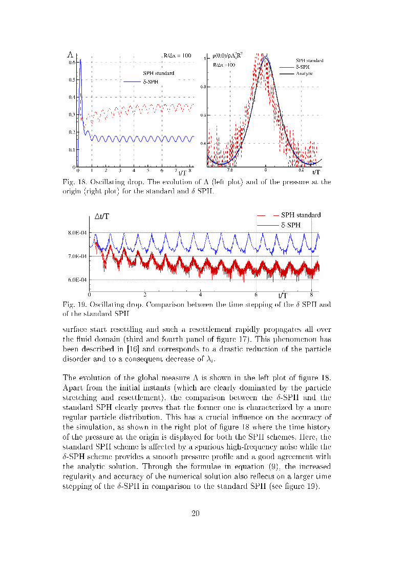
Fig. 18. Oscillating drop. The evolution of Λ (left plot) and of the pressure at theorigin (right plot) for the standard and δ-SPH.

Fig. 19. Oscillating drop. Comparison between the time stepping of the δ-SPH andof the standard SPH

surface start resettling and such a resettlement rapidly propagates all overthe �uid domain (third and fourth panel of �gure 17). This phenomenon hasbeen described in [16] and corresponds to a drastic reduction of the particledisorder and to a consequent decrease of λi.

The evolution of the global measure Λ is shown in the left plot of �gure 18.Apart from the initial instants (which are clearly dominated by the particlestretching and resettlement), the comparison between the δ-SPH and thestandard SPH clearly proves that the former one is characterized by a moreregular particle distribution. This has a crucial in�uence on the accuracy ofthe simulation, as shown in the right plot of �gure 18 where the time historyof the pressure at the origin is displayed for both the SPH schemes. Here, thestandard SPH scheme is a�ected by a spurious high-frequency noise while theδ-SPH scheme provides a smooth pressure pro�le and a good agreement withthe analytic solution. Through the formulae in equation (9), the increasedregularity and accuracy of the numerical solution also re�ects on a larger timestepping of the δ-SPH in comparison to the standard SPH (see �gure 19).

20

Fig. 20. three-dimensional oscillating drop. Sketches of the evolution and contourzones of the pressure �eld (R/∆x = 50). The solid lines represent speci�c sectionsof the analytic free surface.

3.4.1 Extension to three dimensions

The two-dimensional solution provided in the previous section can be easilyextended in three dimensions. In this case the drop evolves like a spheroid,according to the following law:

u = −A(t)x

v = −A(t) y

w = 2A(t) z ,

(14)

and the solution for A(t) is given in [20], as well. Similarly to the two-dimensional case, the global dynamics depends on the ratio A(0)/B (whereB is the coe�cient of the central conservative force �eld). In the followingsimulations, this ratio is set equal to 1.

Figure 20 shows some snapshots of the evolution along with the contour zonesof the pressure �eld obtained by using the δ-SPH scheme. For graphicalreasons, only half of the �uid domain is displayed while the solid linesrepresent speci�c sections of the analytic free surface. The circular dropinitially stretches along the vertical direction in form of a prolate spheroid(left panel of �gure 20), reaches the maximum elongation (central panel) and,then, shrinks to form an oblate spheroid (right panel of the same �gure). Inall the cases, the numerical solution is in a good agreement with the analyticsolution for the free surface.

The procedure used to build the disorder measure Λ can be straightforwardly

21

Fig. 21. three-dimensional oscillating drop. Evolution of the measure Λ andcomparison with the two-dimensional problem.

applied to the three dimensional problem. In this case it is interesting tocompare the evolution of Λ with the two dimensional simulation (see �gure21). In three dimensions the time history of Λ does not exhibit the initialpeak since the particle resettlement is weaker. Intuitively, this is due to thefact that in three dimensions particles have more degrees of freedom and,consequently, they rearrange previously than the two dimensional case andwith weaker dynamics. Apart from this, the long time evolution is similar inboth the cases.

Conclusions

Based only on geometrical considerations, we proposed an algorithm tomeasure the disorder in a generic particle distribution. The proposed measureapplies to both two- and three-dimensional problems and can be qualitativelyregarded as the mean absolute value of the perturbation with respect to ahypothetical regular lattice.

Possible practical applications of the proposed disorder measure have beenprovided by using the Smoothed Particle Hydrodynamics scheme andconsidering both two- and three-dimensional simulations. The numericalsimulations highlighted how Λ can be used to inspect the relation between theparticle disorder and the accuracy of the numerical scheme and to comparedi�erent variants of the same numerical method. The proposed measure maybe also adopted to monitor the particle disorder during simulations and decidewhen/if re-meshing or packing algorithms have to be used. This would help tooptimize the implementation of such tools, reducing the computational costs.

In all the considered cases, the disorder measure proved to be reliableand to qualitatively discriminates between more and less regular particledistributions.

22

Acknowledgments

This work has been also funded by the Flagship Project RITMARE - TheItalian Research for the Sea - coordinated by the Italian National ResearchCouncil and funded by the Italian Ministry of Education, University andResearch within the National Research Program 2011-2014.

A Random noise on a regular lattice

Let us consider a regular grid with uniform spacing ∆x and two independentrandom variables, say x and y, with the same density distribution and withzero mean, that is E(x) = E(y) = 0. Starting from them, we derive twonew independent variables, namely X and Y , with the same probabilitydistribution of x and y, with zero mean and which satisfy:

E(Z) = E(√

X2 + Y 2)

= εr ∆x . (A.1)

Here εr is assigned and represents the mean absolute relative error with respectto the regular grid. The variables X and Y are used to perturb the horizontaland vertical coordinates of the grid points of the regular lattice.

The derivation of X and Y is straightforward. We introduce a positiveparameter α and set X = αx and Y = α y. By de�nition, X and Y havethe same probability distribution of x and y, are independent and have zeromean. The parameter α is obtained by satisfying the requirement in (A.1):

E(Z) = αE(√

x2 + y2)

= εr ∆x ⇒ α =εr ∆x

E(√

x2 + y2) .

It is simple to show that the variance of the new variables is V(X) = α2V(x)and V(Y ) = α2V(y). Then, the larger the relative error εr, the larger thevariance. In our computations we use a Normal Gaussian distribution and aUniform distribution in [0, 1] for x and y.

References

[1] S. R. Idelsohn, E. Oñate, F. Del Pin. The particle �nite element method: apowerful tool to solve incompressible �ows with free-surfaces and breaking waves,International Journal for Numerical Methods in Engineering, 61: 964-989 (2004).

23

[2] J.J. Monaghan, Smoothed Particle Hydrodynamics, Rep. Prog. Phys. 68, 1703�1759, (2005).

[3] G. H. Cottet & P. D. Koumoutsakos, Vortex Methods: Theory and Practice,Cambridge University Press, March 13-th, 2000

[4] P. D. Koumoutsakos, Multiscale Flow Simulations using Particles, Annu. Rev.Fluid Mech. 37: 457-487, 2005.

[5] N. J. Quinlan, M. Basa, M. Lastiwka, Truncation error in mesh-free particlemethods, Int. J. Numer. Meth. Engng., 66: 2064-2085 (2006)

[6] A. K. Chaniotis, D. Poulikakos, P. Koumoutsakos, Remeshed SmoothedParticle Hydrodynamics for the Simulation of Viscous and Heat ConductingFlows, Journal of Computational Physics, 182(1): 67-90, 2002.

[7] S. Børve, M. Omanq, J. Trulsen, Regularized smoothed particle hydrodynamics:a new approach to simulating magneto-hydrodynamic shocks, Astrophys. J., 561,82-93, (2001)

[8] S. J. Lind, R. Xu, P. K. Stansby, B. D. Rogers, Incompressible smoothed particlehydrodynamics for free-surface �ows: A generalised di�usion-based algorithm forstability and validations for impulsive �ows and propagating waves, J. Comput.Phys., 231(4), 1499-1523, (2012)

[9] R. Vacondio, B. D. Rogers, P. K. Stansby, Smoothed Particle Hydrodynamics:Approximate zero-consistent 2-D boundary conditions and still shallow-watertests, Int. J. Num. Meth. Fluids, 69(1), 226-253, (2012)

[10] J. J. Monaghan and R. A. Gingold, Shock simulation by the particle methodSPH, J. Comput. Phys., 52(2), 374-389, (1983)

[11] A. Colagrossi, M. Antuono, A. Souto-Iglesias, D. Le Touzé, David, Theoreticalanalysis and numerical veri�cation of the consistency of viscous smoothed-particle-hydrodynamics formulations in simulating free-surface �ows, PhysicalReview E, 84(2), 026705, (2011)

[12] A. Colagrossi, A meshless lagrangian method for free-surface and interface �owswith fragmentation, PhD Thesis, Università degli Studi di Roma �La Sapienza�,2005

[13] A. Amicarelli, J-C. Marongiu, F. Leboeuf, J. Leduc, M. Neuhauser, L. Fang, J.Caro, SPH truncation error in estimating a 3D derivative, International Journalfor Numerical Methods in Engineering, 87(7), 677-700, (2011)

[14] A. Amicarelli, J-C. Marongiu, F. Leboeuf, J. Leduc, J. Caro, SPH truncationerror in estimating a 3D function, Computers & Fluids , 44(1), 279-296, (2011)

[15] A. Colagrossi, B. Bouscasse, M. Antuono, S. Marrone, Particle packing algorithmfor SPH schemes, Computer Physics Communications, 183, 1641-1653, (2012)

[16] D. Le Touzé, A. Colagrossi, G. Colicchio, M. Greco, A critical investigationof Smoothed Particle Hydrodynamics applied to problems with free surfaces,International Journal of Numerical Methods in Fluids, 73, 660-691, (2013)

24

[17] G. I. Taylor and A. E. Green, Mechanism of the Production of Small Eddiesfrom Large Ones, Proc. R. Soc. Lond. A, 158, 499-521 (1937).

[18] R. Xu, P. K. Stansby, D. Laurence, Accuracy and stability in incompressibleSPH (ISPH) based on the projection method and a new approach, J. Comput.Phys., 228(18), 6703-6725, (2009)

[19] R. Vacondio, B. D. Rogers, P. K. Stansby, P. Mignosa, A correction for balancingdiscontinuous bed slopes in two-dimensional smoothed particle hydrodynamicsshallow water modeling, Int. J. Num. Meth. Fluids, 71(7), 850-872, (2013)

[20] J. J. Monaghan and Ashkan Ra�ee, A simple SPH algorithm for multi-�uid �owwith high density ratios, Int. J. Numer. Meth. Fluids, 71: 537-561 (2013)

[21] M. Antuono, A. Colagrossi, S. Marrone, Numerical di�usive terms in weakly-compressible SPH schemes, Computer Physics Communications 183: 2570-2580(2012)

25