
a library decision support system built on data warehousing
73
A LIBRARY DECISION SUPPORT SYSTEM BUILT ON DATA WAREHOUSING AND DATA MINING CONCEPTS AND TECHNIQUES By ASHWIN NEEDAMANGALA A THESIS PRESENTED TO THE GRADUATE SCHOOL OF THE UNIVERSITY OF FLORIDA IN PARTIAL FULFILLMENT OF THE REQUIREMENTS FOR THE DEGREE OF MASTER OF SCIENCE UNIVERSITY OF FLORIDA 2000
-
Upload
khangminh22 -
Category
Documents
-
view
3 -
download
0
Transcript of a library decision support system built on data warehousing

A LIBRARY DECISION SUPPORT SYSTEM BUILT ON DATA WAREHOUSING AND DATA MINING CONCEPTS AND TECHNIQUES
By
ASHWIN NEEDAMANGALA
A THESIS PRESENTED TO THE GRADUATE SCHOOL OF THE UNIVERSITY OF FLORIDA IN PARTIAL FULFILLMENT
OF THE REQUIREMENTS FOR THE DEGREE OF MASTER OF SCIENCE
UNIVERSITY OF FLORIDA
2000

ii
ACKNOWLEDGMENTS
I would like to express my sincere gratitude towards my advisor, Dr. Stanley Su,
for giving me an opportunity to work on this challenging topic and for providing
continuous feedback during the course of this work and thesis writing.
I wish to thank Dr. Limin Fu for his guidance and support during this work and
also for allowing me to use his system, DOMRUL, for data mining purposes. Thanks are
due to Dr. Joachim Hammer for agreeing to be on my committee.
I would also like to thank Phek Su for making this entire work a pleasurable
experience. My thanks go to Sharon Grant for making the Database Center a truly great
place to work. I would also like to thank a number of people at the University of Florida
Library for providing valuable input for this work.
I would like to take this opportunity to thank my parents, my sister, my brother-
in-law and Anu for their constant emotional support and encouragement throughout my
academic career.

iii
TABLE OF CONTENTS
page
ACKNOWLEDGMENTS .................................................................................................. ii
LIST OF TABLES ...............................................................................................................v
LIST OF FIGURES ........................................................................................................... vi
ABSTRACT...................................................................................................................... vii
INTRODUCTION ...............................................................................................................1
SYSTEM DESIGN ..............................................................................................................5
2.1 Environment and Data .............................................................................................. 5 2.1.1 Library Environment.......................................................................................... 5 2.1.2 Library Data Sources ......................................................................................... 5
2.1.2.1 FCLA DB2 tables and key list .................................................................... 6 2.1.2.2 Bibliographic and circulation data extraction ............................................. 6
2.2 System Architecture.................................................................................................. 7 2.2.1 Data Warehousing.............................................................................................. 7
2.2.1.1 NOTIS ......................................................................................................... 7 2.2.1.2 Host Explorer .............................................................................................. 9 2.2.1.3 Screen scraping technique........................................................................... 9 2.2.1.4 Data cleansing and extraction................................................................... 11 2.2.1.5 Data loading.............................................................................................. 11 2.2.1.6 Warehouse architecture............................................................................. 11 2.2.1.7 Data modeling........................................................................................... 14 2.2.1.8 Characteristics of the warehouse............................................................... 16 2.2.1.9 Structure of the warehouse........................................................................ 16
2.2.2 Data Mining ..................................................................................................... 19 2.2.2.1 What is data mining?................................................................................. 19 2.2.2.2 Data mining techniques and processes...................................................... 19 2.2.2.3 Neural networks ........................................................................................ 21 2.2.2.4 Discretization of numeric attributes .......................................................... 24 2.2.2.5 Handling non-numeric attributes .............................................................. 25 2.2.2.6 LDSS mining tool interface (LibMine)..................................................... 27
iv
SYSTEM IMPLEMENTATION.......................................................................................28
3.1 Warehouse Build-time Tools .................................................................................. 28 3.1.1 Graphical User Interface (GUI) ....................................................................... 28 3.1.2 Database Connectivity Issues........................................................................... 30 3.1.3 Screen Scraping................................................................................................ 30 3.1.4 Data Cleansing and Extraction......................................................................... 31 3.1.5 Data Loading Manager..................................................................................... 34
3.2 Warehouse Run-time Tools .................................................................................... 35 3.2.1 Canned Queries ................................................................................................ 36
3.2.1.1 Sample query outputs ................................................................................ 37 3.2.1.2 Report generation...................................................................................... 37
3.2.2 Ad-Hoc Queries ............................................................................................... 39 3.3 Data Mining Build-time Tool ................................................................................. 43
3.3.1 Data Preparation............................................................................................... 43 3.3.1.1 Selection of non-goal attributes (feature vector)....................................... 45 3.3.1.2 Discretization of continuous attributes ..................................................... 45 3.3.1.3 Grouping similar non-numeric attribute values ........................................ 50
3.3.2 Structure of Training Data Set ......................................................................... 53 3.3.3 Sending training data to DOMRUL................................................................. 54
3.4 Data Mining Run-time Tool.................................................................................... 54 3.4.1 DOMRUL ........................................................................................................ 54 3.4.2 Results of test runs ........................................................................................... 56
SUMMARY AND CONCLUSIONS ................................................................................60
LIST OF REFERENCES ...................................................................................................62
BIOGRAPHICAL SKETCH .............................................................................................65

v
LIST OF TABLES
Table Page 3.1 Query 1 Results ................................................................................................................37
3.2 Query 2 Results ................................................................................................................37
3.3 Sample Report..................................................................................................................37
3.4 Query 4 Results ................................................................................................................38
3.5 Query 5 Results ................................................................................................................38
3.6 Sample Data Set ...............................................................................................................47
3.7 Sample Publisher Data Set ...............................................................................................51
vi
LIST OF FIGURES
Figure Page 2.1 LDSS Architecture............................................................................................................8
2.2 Structure of the Library Data Warehouse..........................................................................17
2.3 Classes of Data Mining.....................................................................................................21
2.4 Structure of a Neural Network..........................................................................................22
3.1 A Sample NOTIS Screen..................................................................................................32
3.2 A Text-Delimited File ......................................................................................................34
3.3 Step 1: Ad-Hoc Query Wizard .........................................................................................40
3.4 Step 2: Ad-Hoc Query Wizard .........................................................................................41
3.5 Step 3: Ad-Hoc Query Wizard .........................................................................................42
3.6 Step 4: Ad-Hoc Query Wizard .........................................................................................42
3.7 Query Output.....................................................................................................................43
3.8 Listing of Query Output.....................................................................................................44
3.9 Sample Cluster Tree.........................................................................................................52
vii
Abstract of Thesis Presented to the Graduate School
of the University of Florida in Partial Fulfillment of the Requirements for the Degree of Master of Science
A LIBRARY DECISION SUPPORT SYSTEM BUILT ON DATA WAREHOUSING AND DATA MINING CONCEPTS AND TECHNIQUES
By
Ashwin Needamangala
August, 2000
Chairman: Dr. Stanley Y.W. Su Cochairman: Dr. LiMin Fu Major Department: Electrical and Computer Engineering
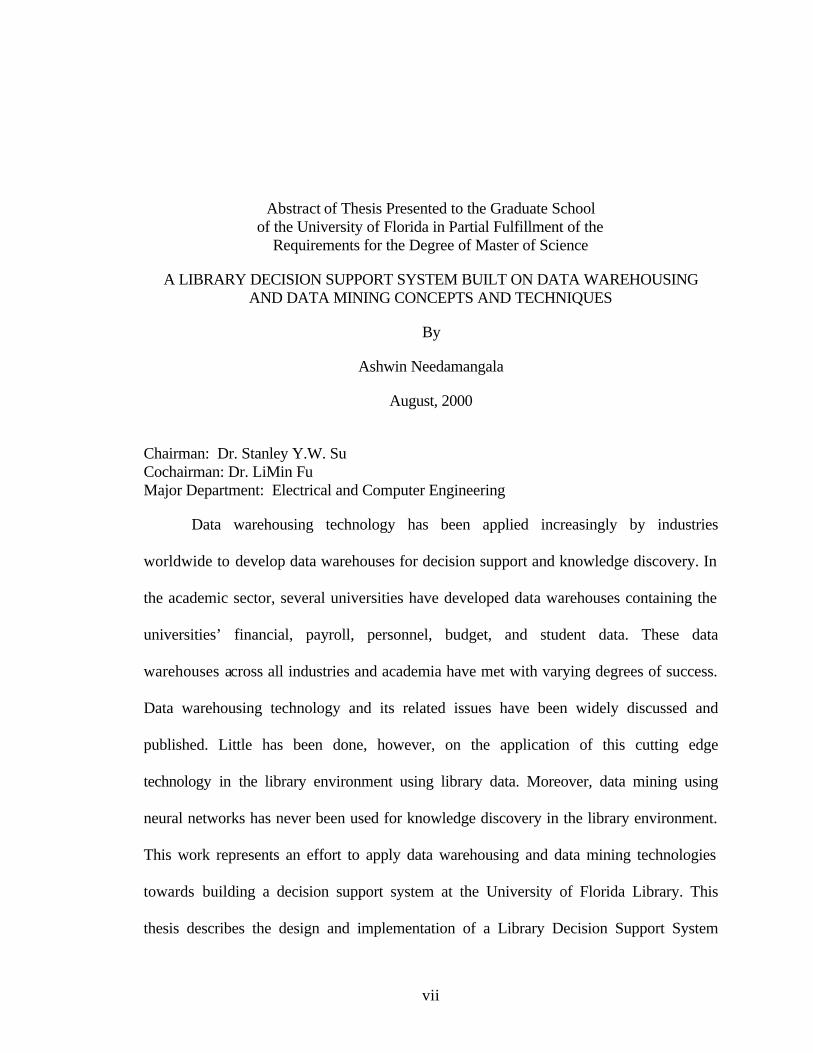
Data warehousing technology has been applied increasingly by industries
worldwide to develop data warehouses for decision support and knowledge discovery. In
the academic sector, several universities have developed data warehouses containing the
universities’ financial, payroll, personnel, budget, and student data. These data
warehouses across all industries and academia have met with varying degrees of success.
Data warehousing technology and its related issues have been widely discussed and
published. Little has been done, however, on the application of this cutting edge
technology in the library environment using library data. Moreover, data mining using
neural networks has never been used for knowledge discovery in the library environment.
This work represents an effort to apply data warehousing and data mining technologies
towards building a decision support system at the University of Florida Library. This
thesis describes the design and implementation of a Library Decision Support System

viii
(LDSS). LDSS offers querying tools by means of which the library management can
perform financial analysis and, thereby, make the expenditure of the library budget
efficient. The LDSS also aids book selectors in decision making by using its data mining
component, LibMine.
1
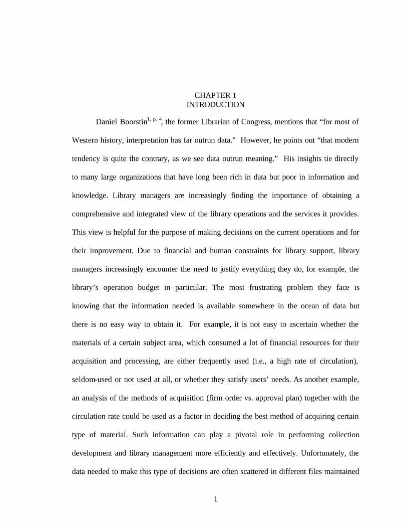
CHAPTER 1 INTRODUCTION
Daniel Boorstin1, p. 4, the former Librarian of Congress, mentions that “for most of
Western history, interpretation has far outrun data.” However, he points out “that modern
tendency is quite the contrary, as we see data outrun meaning.” His insights tie directly
to many large organizations that have long been rich in data but poor in information and
knowledge. Library managers are increasingly finding the importance of obtaining a
comprehensive and integrated view of the library operations and the services it provides.
This view is helpful for the purpose of making decisions on the current operations and for
their improvement. Due to financial and human constraints for library support, library
managers increasingly encounter the need to justify everything they do, for example, the
library’s operation budget in particular. The most frustrating problem they face is
knowing that the information needed is available somewhere in the ocean of data but
there is no easy way to obtain it. For example, it is not easy to ascertain whether the
materials of a certain subject area, which consumed a lot of financial resources for their
acquisition and processing, are either frequently used (i.e., a high rate of circulation),
seldom-used or not used at all, or whether they satisfy users’ needs. As another example,
an analysis of the methods of acquisition (firm order vs. approval plan) together with the
circulation rate could be used as a factor in deciding the best method of acquiring certain
type of material. Such information can play a pivotal role in performing collection
development and library management more efficiently and effectively. Unfortunately, the
data needed to make this type of decisions are often scattered in different files maintained

2
by a large centralized system such as NOTIS, which does not provide a general querying
facility, or by different file/data management or application systems. This situation makes
it very difficult and time-consuming to extract useful information from them. This is
precisely where data-warehousing technology comes in.
The goal of this research and development work is to apply data warehousing and
data mining technologies in the development of a Library Decision Support System
(LDSS) to aid in the library management’s decision making. The first phase of this work
is to establish a data warehouse by importing selected data from separately maintained
files presently used in the George A. Smathers Libraries of the University of Florida into
a relational database system (Microsoft Access). Data stored in the existing files were
extracted, cleansed, aggregated and transformed into the relational representation suitable
for processing by the relational database management system. A Graphical User
Interface (GUI) is developed to allow decision makers to query for the data warehouse’s
contents using either some pre-defined queries or ad-hoc queries. Our goal is to develop a
general methodology and inexpensive software tools, which can be used by different
functional units of a library to import data from different data sources and to tailor
different warehouses to meet their local decision needs. For meeting this objective, we do
not have to use a very large centralized database management system to establish a single
very large data warehouse to support different uses.
The second objective is to apply data mining techniques on the library data
warehouse for knowledge discovery. But as is well known, data mining can only give
answers. As for the questions, the user needs to formulate them first. So we had to come
up with questions for which the library did not have concrete answers. The questions

3
were almost all pertaining to the financial domain since efficient expenditure of the
library’s budget is extremely important. It was observed that the expenditure of the
library budget was directly linked to the book selection process. One of the most
troublesome questions faced by the library management is as follows:
• How do we know during the selection process if a particular book is going to be
worth selecting or not?
The book selection process is a very intricate one. Book selectors consider it to be
more of an art than a science. But if there were to be a tool that could use past data on
book selection and, thereby, generate rules for the present and future, the selector’s job
would be made a lot easier. It would be entirely up to the selector to define the factors
that determine the worth of a book bought in the past since these factors might differ
from selector to selector. Rule generation can be performed in a number of ways. But in
order to achieve our objective as well as respect the selectors’ opinion, we needed to
model the rule generation mechanism as closely as possible to the selection process of the
selectors. This was the reason for deciding to use neural networks for rule generation in
this work.
In this thesis, we describe the design and implementation of a Library Decision
Support System (LDSS). Library data is collected from various sources using means such
as screen scraping. The data is then loaded into a data warehouse maintained in
Microsoft Access. The user is provided with both canned queries as well as the Ad-Hoc
Query Wizard as decision-support tools. The user can also compose a training data set to
be submitted to a neural network (DOMRUL) which in turn learns domain rules from the
submitted data. These rules can be used for prediction of the popularity of a particular
4
book. Both discretization and clustering algorithms, which are required during the
process of composing the training data set, have been implemented.
This thesis is organized as follows. The next chapter contains a detailed
discussion on the design of the Library Decision Support System (LDSS), describing the
system architecture, warehouse architecture and design of the mining tool. Chapter 3
describes the implementation details of the LDSS. The summary and conclusions are
given in Chapter 4.
5
CHAPTER 2 SYSTEM DESIGN
This chapter presents the design of the Library Decision Support System (LDSS)
and discusses some design issues.
2.1 Environment and Data
2.1.1 Library Environment
The University of Florida Libraries has a holding of over two million titles,
comprising over three million volumes. It shares a NOTIS-based integrated system with
nine other State University System (SUS) libraries for acquiring, processing, circulating
and accessing its collection. All the ten SUS libraries are under the consortium umbrella
of the Florida Center for Library Automation (FCLA).
2.1.2 Library Data Sources
The University of Florida Libraries’ online database, LUIS, stores a wealth of
data, such as bibliographic data (author, title, subject, publisher information), acquisitions
data (price, order information, fund assignment), circulation data (charge out and browse
information, withdrawn and inventory information), and owning location data (where
item is shelved). These voluminous data are stored in separate files.
The Library Decision Support System (LDSS) is developed with the capability of
handling and analyzing an established data warehouse. For testing our methodology and
software system, we established a warehouse based on twenty thousand monograph titles
acquired from our major monograph vendor. These titles were published by domestic

6
U.S. publishers and have a high percentage of DLC/DLC records (titles cataloged by the
Library of Congress). They were acquired by firm order and approval plan. The
publication coverage is the calendar year 1996-1997. Analysis is only on the first item
record (future work will include all copy holdings). Although the size of the test data
used is small, it is sufficient to test our general methodology and the functionality of our
software system.
2.1.2.1 FCLA DB2 tables and key list
Most of the data from the 20,000-title domain that go into the LDSS warehouse
are obtained from the DB2 tables maintained by FCLA. FCLA developed and maintains
the database of a system called Ad-Hoc Report Request Over the Web, ARROW2 to
facilitate querying and generating reports on acquisitions activities. The data are stored
in DB2 tables.
For our R&D purpose, we need DB2 tables for only the 20,000 titles that we have
identified as our initial project domain. These 20,000 titles all have an identifiable 035
field in the bibliographic records (zybp1996, zybcip1996, zybp1997 or zybpcip1997).
We use the BatchBAM program3 developed by Gary Strawn of Northwestern University
Library to extract and list the unique bibliographic record numbers in separate files.
Using the unique bibliographic record numbers, FCLA extracted the DB2 tables from the
ARROW database and exported the data to text files.
2.1.2.2 Bibliographic and circulation data extraction
FCLA collects and stores as DB2 tables complete acquisitions data from the order
records. However, only brief bibliographic data and no item record data are available.
Bibliographic and item record data are essential for inclusion in the LDSS warehouse in
order to create a viable integrated system capable of performing cross-file analysis and
7
querying for the relationships among different types of data. Because these required data
do not exist in any computer readable form, we designed a method to obtain them. Using
the identical NOTIS key lists to extract4 the targeted 20,000 bibliographic and item
records, we applied a screen scraping technique to scrape the data from the screen and
saved them in a flat file.
2.2 System Architecture
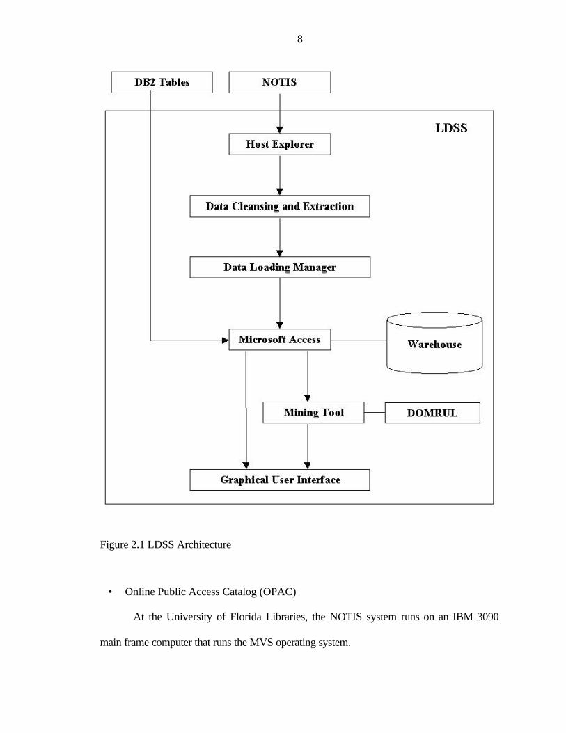
The architecture of the LDSS system is shown in Figure 2.1. There are two main
technologies involved in the LDSS; namely, data warehousing and data mining. We shall
discuss them separately and present the system components and their function.
2.2.1 Data Warehousing
The components that are used to construct and query the warehouse are given
below.
2.2.1.1 NOTIS
NOTIS is an acronym for Northwestern Online Totally Integrated System. The
NOTIS system was developed at Northwestern University Library and introduced in
1970. Since its inception, NOTIS has undergone many versions. University of Florida
Libraries is one of the earliest users of NOTIS. FCLA has made many local
modifications of the NOTIS system since UF Libraries started using it. As a result, the
UF NOTIS is different from the rest of the NOTIS world in many respects. NOTIS can
be broken down into four sub-systems:
• Acquisitions
• Cataloging
• Circulation
8
Figure 2.1 LDSS Architecture
• Online Public Access Catalog (OPAC)
At the University of Florida Libraries, the NOTIS system runs on an IBM 3090
main frame computer that runs the MVS operating system.
9
2.2.1.2 Host Explorer
Host Explorer is a software program that provides a TCP/IP link to the main
frame computer. It is a terminal emulation program supporting the IBM main frame,
AS/400 and VAX hosts. Host Explorer delivers an enhanced user environment for all
Windows NT platforms, Windows 95 and Windows 3.x desktops. Exact TN3270E,
TN5250, VT420/320/220/101/100/52, WYSE 50/60 and ANSI-BBS display is extended
to leverage the wealth of the Windows desktop. It also supports all TCP/IP based
TN3270 and TN3270E gateways.
The Host Explorer program is used as the terminal emulation program in LDSS.
It also provides VBA compatible BASIC scripting tools for complete desktop macro
development. Users can run these macros directly or attach them to keyboard keys,
toolbar buttons and screen hotspots for additional productivity. The function of Host
Explorer in the LDSS is very simple. It has to “visit” all screens in the NOTIS system
corresponding to each NOTIS number present in the BatchBam file, and capture all the
data on the screens. In order to do this, we wrote a macro in the Visual Basic for
Applications (VBA) programming language. Upon completion of the scraping, all the
data scraped from the NOTIS screen reside in a flat file. The data present in this file have
to be cleansed in order to make them suitable for insertion into the Library Warehouse.
2.2.1.3 Screen scraping technique
Screen scraping is a process used to capture data from a host application. It is
conventionally a three-part process:
• Displaying the host screen or data that you want to scrape.
• Finding the screen location of the data that you want to capture.
10
• Capturing the data to a PC or host file, or using them in another Windows
application.
In other words, we can capture particular data on the screen by providing the
corresponding screen coordinates to the screen-scraping program. Numerous commercial
applications for screen scraping are available in the market. However, we used an
approach slightly different from the conventional one. Although we had to capture only
certain fields from the NOTIS screen, there were other factors that we had to take into
consideration. They are
• The location of the various fields with respect to the screen coordinates changes
from record to record. This makes it impossible for us to lock a particular field with
a corresponding screen coordinate.
• The data present on the screen are dynamic because we are working on a “live”
database where data are frequently modified. For accurate query results, all the data,
especially the item record data where the circulation transactions are housed, need
to be captured within a specified time interval so that the data are uniform. This
makes the time taken for capturing the data extremely important.
• Most of the fields present on the screen needed to be captured for data warehousing
and mining purposes.
Taking the above factors into consideration, it was decided to capture the entire
screen instead of scraping only certain part of the screen. This made the process both
simpler and faster. The unnecessary fields were filtered out during the cleanup process.

11
2.2.1.4 Data cleansing and extraction
Some data present on the NOTIS screen are unnecessary from the point of view of
this project. We need only certain fields from the NOTIS screen. Even in these fields,
only some data delimited by some delimiters are of interest to us. Therefore, we wrote a
program to scan each field against a pre-defined set of delimiters. The data delimited by
other delimiters are discarded. The Data Cleansing Tool of the LDSS is written in Java.
Its main function is to cleanse the data that have been scraped from the NOTIS screen. It
saves the cleansed data in a text-delimited format that is recognized by Microsoft Access.
This file is then imported into the Library Warehouse maintained by Microsoft Access.
2.2.1.5 Data loading
Once the scraped data have been cleansed, the data are ready to be loaded into the
data warehouse. The Data Loading Manager of the LDSS performs this task. FCLA
exports the data existing in the DB2 tables into text files. As a first step towards creating
the warehouse database, these text files are transferred using FTP and form separate
relational tables in the Library Warehouse. The data that are scraped from the
bibliographic and item record screens result in the formation of two more tables. The
main function of the Data Loading Manager is to load these scraped data into the
warehouse database.
2.2.1.6 Warehouse architecture
Architecture Choices
In this section we discuss the architecture choices available for the data
warehouse. The architecture choice selected is a management decision that should be
based on such factors as the current infrastructure, business environment, desired
management and control structure, commitment to and scope of the implementation
12
effort, capability of the technical environment the organization employs, and resources
available. Selection of an architecture will determine, or be determined by, where the data
warehouses will reside and where the control resides. For example, the data can reside in
a central location that is managed centrally. Or, the data can reside in distributed local
and/or remote locations that are either managed centrally or independently. The common
architecture choices5-17 are discussed in brief below.
• Global Warehouse Architecture
A global data warehouse is considered to be one that will support all, or a large part
of an organization that requires a more fully integrated data warehouse with a high degree
of data access and usage. That is, it is designed and constructed based on the needs of the
organization as a whole. It can be considered as a common repository for decision
support that is available across the entire organization or a large subset thereof. Data for
the data warehouse is typically extracted from operational systems and possibly from data
sources external to the organization with batch processes during off-peak operational
hours. It is then filtered to eliminate any unwanted data items and transformed to meet the
data quality and usability requirements. It is then loaded into the appropriate data
warehouse databases for access by end users. A global warehouse architecture enables
end users to have more of an organization-wide view of the data.
• Independent Data Mart Architecture
An independent data mart architecture implies stand-alone data marts that are
controlled by a particular workgroup, department, or line of business and are built solely
to meet their needs. In fact, there may not even be any connectivity with data marts in
other workgroups, departments, or lines of business. The data for these data marts may be
13
generated internally. Data could also be extracted from sources of data external to the
organization. The data in any particular data mart will be accessible only to those in the
workgroup, department, or line of business.
• Interconnected Data Mart Architecture
An interconnected data mart architecture is basically a distributed implementation.
Although separate data marts are implemented in a particular workgroup, department, or
line of business, they can be integrated, or interconnected, to provide a more
organization-wide view of the data. Therefore, end users in one department can access
and use the data on a data mart in another department. Interconnected data marts can be
independently controlled by different workgroups, departments, or lines of business, each
of which decides what source data to load into its data mart, when to update it, who can
access it, and where it resides.
Chosen Architecture
In this section we specify our choice of a warehouse architecture and explain
some of the considerations involved in the selection decision.
At present, the University of Florida Library does not have a robust infrastructure
that can support a full-fledged data warehouse. It does not have a sophisticated technical
environment either. These facts need to be taken into consideration when we choose the
warehouse architecture. As a result, we cannot afford to choose either of the data mart
architectures which are relatively more complex than the global warehouse architecture.
The architecture of the warehouse is affected by the nature of target end-users of
the warehouse. Our target end-users are the upper level management at the University of
Florida Library. As has been mentioned before, one of the main uses of the LDSS will be

14
to aid in efficient expenditure of the library budget. Only the upper level management
decides the expenditure of the budget and so they form the set of target end-users. In that
case, since we do not have different subsets of end-users, there is no need to choose any
of the data mart architecture models. The global warehouse architecture would be a
perfect fit considering the fact that we have a single large set of end-users.
The library has very limited resources both in terms of hardware and software.
These limitations need to be taken into consideration while choosing the warehouse
architecture. This limitation also points to choosing the global warehouse architecture
over the data mart architectures. The implementation of any of the data mart architectures
would require sophisticated hardware as well as software.
Taking all of the above factors into consideration, we decide to opt for the global
warehouse architecture. Now we need to decide on the methodology to be followed for
warehouse implementation.
2.2.1.7 Data modeling
Data warehousing has become generally accepted as the best approach for
providing an integrated, consistent source of data for use in data analysis and business
decision making. Whether you approach data warehousing from a global perspective or
begin by implementing data marts, the benefits from data warehousing are significant.
The question then becomes, How should the data warehouse databases be designed to
best support the needs of the data warehouse users? Answering that question is the task of
the data modeler. Data modeling is, by necessity, part of every data processing task, and
data warehousing is no exception. There are two basic data modeling techniques that can
be followed: ER modeling and dimensional modeling. We now proceed to perform a
brief comparison of these two techniques.
15
Data Modeling Techniques
Two data modeling techniques that are relevant in a data warehousing
environment are ER modeling and dimensional modeling.
In the operational environment, the ER modeling technique has been the
technique of choice. ER modeling produces a data model of the specific area of interest,
using two basic concepts: entities and the relationships among these entities. Detailed ER
models also contain attributes, which can be properties of either entities or relationships.
The ER model is an abstraction tool, which can be used to model the complex
relationships among data entities and their properties.
Dimensional modeling uses three basic concepts: measures, facts, and
dimensions. Dimensional modeling is powerful in representing the requirements of the
business user in the context of database tables.
Both ER and dimensional modeling can be used to create an abstract model of a
specific subject. However, each has its own limited set of modeling concepts and
associated notation conventions. Consequently, the techniques look different, and they
are indeed different in terms of semantic representation.
The LDSS is designed for use by a relatively small group of people who deal with
data in some specific domains. We want to make this system available to many groups,
each of which can install the software on their PCs and Microsoft Access is a suitable
DBMS for use to manage the individual warehouses. It is extremely complex to perform
dimensional modeling in Microsoft Access. As a result, we chose ER modeling over
dimensional modeling.

16
2.2.1.8 Characteristics of the warehouse
Data in the warehouse are snapshots of the original data files. Only a subset of the
data contents in these files are extracted for querying and analysis since not all the data
are useful for a particular decision-making situation. Data are filtered as they pass from
the operational environment to the data warehouse environment. This filtering process is
necessary particularly when a PC system, which has limited secondary storage and main
memory space, is used. Once extracted and stored in the warehouse, data are not
updateable. They form a read-only database. However, different snapshots of the original
files can be imported into the warehouse for querying and analysis. The results of the
analyses of different snapshots can then be compared.
2.2.1.9 Structure of the warehouse
Data warehouses have a distinct structure. There are summarization and detail
structures that demarcate a data warehouse. The structure of the Library Data Warehouse
is shown in Figure 2.2. The different components of the Library Data Warehouse are:
• NOTIS and DB2 Tables
NOTIS is an acronym for Northwestern Online Totally Integrated System. A brief
description of NOTIS has been provided in Section 2.2.1.1. The bibliographic and
circulation data are obtained from NOTIS through the screen scraping process and
imported into the warehouse. FCLA maintains acquisitions data in the form of DB2
tables. These are also imported into the warehouse after conversion to a suitable format.
• Warehouse Database
The warehouse database consists of several relational tables that are inter-
connected by keys and foreign keys, which specify relationships among relational entity
types.

17
Figure 2.2 Structure of the Library Data Warehouse
The “Universal Relation” approach could have been used to implement the warehouse
database by using a single table. The argument for using the “Universal database by using
a single table. The argument for using the “Universal Relation” approach would be that
all the collected data fall under the same domain. But let us examine why this approach
would not have been suitable. The different data collected for import into the warehouse
were bibliographic data, circulation data, order data, pay data etc. Now, if all these data
were incorporated into one single table with many attributes, it would not be of any
exceptional use since each set of attributes have their own unique meaning when grouped

18
together as Bibliographic Table, Circulation Table and so on. For example, if we group
the circulation data and the pay data together in a single table, it would not make sense.
However, the pay data and the circulation data are related through the Bib_key. Hence,
our use of the conventional approach of having several tables inter-connected by means
of relationships is more appropriate.
• Views
A view in SQL terminology is a single table that is derived from other tables. These
other tables could be base tables or previously defined views. A view does not
necessarily exist in physical form; it is considered a virtual table, in contrast to base
tables whose tuples are actually stored in the database. In the context of the LDSS, views
can be implemented by means of the Ad-Hoc Query Wizard. The user can define a
query/view using the Wizard and save it for future use. The user can then define a query
on this query/view.
• Summarization
The process of implementing views falls under the process of summarization.
Summarization provides the user with views, which makes it easier for users to query on
the data of their interests.
As explained above, the specific warehouse database we established consists of
five tables. Table names including “_WH” indicates that it is current detailed data of the
warehouse. Current detailed data represents the most recent snapshot of data that has
been taken from the NOTIS system. The summarized views are derived from the current
detailed data of the warehouse. Since current detailed data of the warehouse is the basic
data of the application, only the current detailed data tables are shown in Appendix A.
19
2.2.2 Data Mining
So far, we have discussed all the issues involved in the design of the data
warehouse. Now let us discuss the data mining aspect of the Library Decision Support
System. But before we do that, let us briefly review data mining18-19 in general.
2.2.2.1 What is data mining?
There are many good definitions of the term “Data Mining” but the core concept
behind all of them is the same. IBM defines Data Mining as, “the process of extracting
previously unknown, valid and actionable information from large databases and then
using the information to make crucial business decisions”20.
First, the information is previously unknown in that it is not directly derived
from the data – as is something like “total sales”. Instead, the information takes the form
of relationships amongst the database columns where the value in one or more columns
predicts the outcome in another – hence the name, predictive model.
But predictive models must be valid. Rating a model’s predictive power usually
involves testing it against another data set.
Finally, it goes without saying that the information is actionable . But this does
suggest that there should be some goal in mind before putting any effort into data mining.
2.2.2.2 Data mining techniques and processes
While a myriad of approaches to data mining has been proposed, just a few
fundamental techniques form the basis of most systems. Traditionally, there have been
two types of statistical analyses: confirmatory analysis and exploratory analysis21. In
confirmatory analysis, one has a hypothesis and either confirms or refutes it. However,
the bottleneck for the confirmatory analysis is the shortage of hypotheses on the part of

20
the analyst. In “exploratory analysis” one finds suitable hypotheses to confirm or refute.
Here the system takes the initiative in data analysis, not the user.
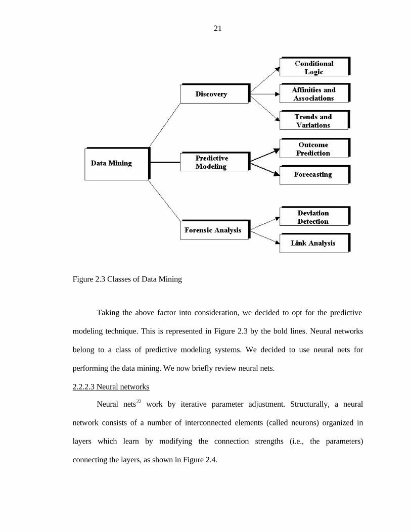
From a process-oriented view, there are three classes of data mining activity:
discovery, predictive modeling and forensic analysis, as shown below in Figure 2.321.
Discovery is the process of looking in a database to find hidden patterns without a
predetermined idea or hypothesis about what the patterns may be. In other words, the
program takes the initiative in finding what the interesting patterns are, without the user
thinking of the relevant questions first. In large databases, there are so many patterns that
the user can never practically think of the right questions to ask. The key issue here is the
richness of the patterns that can be expressed and discovered and the quality of the
information delivered – determining the power and usefulness of the discovery technique.
In predictive modeling, patterns discovered from the database are used to predict
the future. Predictive modeling allows the user to submit records with some unknown
field values, and the system will guess the unknown values based on previous patterns
discovered from the database. While discovery finds patterns in data, predictive modeling
applies the patterns to guess values for new data items.
Forensic analysis is the process of applying the extracted patterns to find
anomalous or unusual data elements. To discover the unusual, we first find what is the
norm, and then we detect those items that deviate from the usual within a given threshold.
With respect to the library environment, we have a specific goal in mind, which is
efficient expenditure of the library budget. This goal spawns relevant questions such as
“Is this book going to be worth buying?” Answering this question demands that we
predict the future based on past data and patterns we have discovered from past data.
21
Figure 2.3 Classes of Data Mining
Taking the above factor into consideration, we decided to opt for the predictive
modeling technique. This is represented in Figure 2.3 by the bold lines. Neural networks
belong to a class of predictive modeling systems. We decided to use neural nets for
performing the data mining. We now briefly review neural nets.
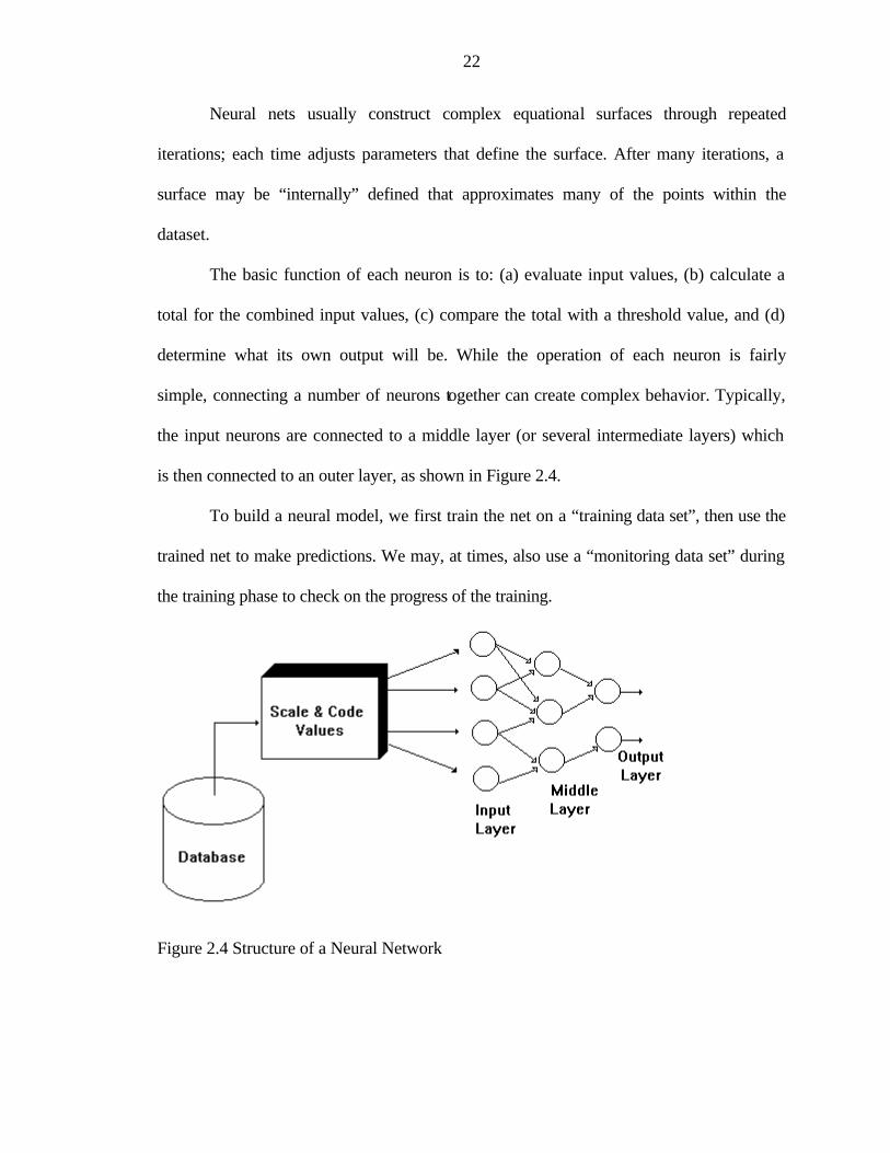
2.2.2.3 Neural networks
Neural nets22 work by iterative parameter adjustment. Structurally, a neural
network consists of a number of interconnected elements (called neurons) organized in
layers which learn by modifying the connection strengths (i.e., the parameters)
connecting the layers, as shown in Figure 2.4.
22
Neural nets usually construct complex equational surfaces through repeated
iterations; each time adjusts parameters that define the surface. After many iterations, a
surface may be “internally” defined that approximates many of the points within the
dataset.
The basic function of each neuron is to: (a) evaluate input values, (b) calculate a
total for the combined input values, (c) compare the total with a threshold value, and (d)
determine what its own output will be. While the operation of each neuron is fairly
simple, connecting a number of neurons together can create complex behavior. Typically,
the input neurons are connected to a middle layer (or several intermediate layers) which
is then connected to an outer layer, as shown in Figure 2.4.
To build a neural model, we first train the net on a “training data set”, then use the
trained net to make predictions. We may, at times, also use a “monitoring data set” during
the training phase to check on the progress of the training.
Figure 2.4 Structure of a Neural Network

23
Each neuron usually has a set of weights that determine how it evaluates the
combined strength of the input signals. Inputs coming into a neuron can be either positive
(excitatory) or negative (inhibitory). Learning takes place by changing the weights used
by the neuron in accordance with classification errors that were made by the net as a
whole. The inputs are usually scaled and normalized to produce a smooth behavior.
Neural nets can be trained to reasonably approximate the behavior of functions on
small and medium sized data sets since they are universal approximators. With respect to
our library project, we have to train the neural net to approximate the behavior of the
book selectors. The training data sets have to be prepared from the data warehouse, which
contains past data on book selection, book circulation and various other factors. The
preparation of the training data sets needs to be performed with utmost care since all the
factors that have affected the book selectors in their decision have to be taken into
consideration during the preparation process. Only then will we get correct results from
the neural net. There are other issues involved with the process of data preparation, as we
will now see.
Since input to a neural net has to be numeric (Boolean), interfacing to a large data
warehouse may become a problem. For each data field used in a neural net, we need to
perform discretization and coding. The numeric or continuous fields are discretized. The
user decides the number of intervals and the data field is then discretized to fit those
intervals. For example, if the charges field needs to be discretized into three intervals, we
can assign three categories as low, medium and high with the suitable intervals. These
intervals need to be selected with care by means of a mathematical process. We now
review the discretization process.
24
2.2.2.4 Discretization of numeric attributes
Discretization23 is performed by dividing the values of a numeric (continuous)
attribute into a small number of intervals, where each interval is mapped to a discrete
(categorical, nominal, symbolic) symbol. For example, if the attribute in question is
charges one possible discretization is: [0…3] � low, [4…8] � medium, [9…�] � high.
Few classification algorithms perform discretization automatically; rather it is the user’s
responsibility to define a discretization and construct a data file containing only discrete
values. While the extra effort of manual discretization is a hardship, of much greater
importance is that the classification algorithm might not be able to overcome the
handicap of poorly chosen intervals. In general, unless users are knowledgeable about the
problem domain and understand the behavior of the classification algorithm they will not
know which discretization is best. So the discretization manager of the LDSS needs to
choose intervals carefully such that some pre-chosen benchmark is maximized. There are
various methods that we can employ for discretization.
The most obvious simple method, called equal-width-intervals, is to divide the
number line between the minimum and maximum values into N intervals of equal size (N
being a user-supplied parameter). Thus, if A and B are the low and high values,
respectively, then the intervals will have width W = (B –A)/N and the interval boundaries
will be at A + W, A + 2W,…, A + (N – 1)W. In a similar method, called equal-frequency-
intervals, the interval boundaries are chosen so that each interval contains approximately
the same number of training examples; this, if N = 10, each interval would contain
approximately 10% of the examples. In addition to these pure discretization processes,
there also exist classification algorithms that perform the discretization dynamically as
the algorithm runs as opposed to discretization being a pre-processing step. One such
25
classification algorithm is the C4.5 algorithm. The C4.5 algorithm is a member of the ID3
family of decision tree algorithms. In C4.5 the same measure used to choose the best
attribute to branch on at each node of the decision tree (usually some variant of
information gain) is used to determine the best value for splitting a numeric attribute into
two intervals. This value, called a cutpoint, is found by exhaustively checking all possible
binary splits of the current interval and choosing the splitting value that maximizes the
information gain measure. However, it is not obvious how such a technique should be
used or adapted to perform discretization when more than two intervals per attribute are
desired. The D-2 algorithm is a possible extension, which applies the above binary
method recursively, splitting intervals as long as the information gain of each split
exceeds some threshold and a limit on the maximum number of intervals has not been
exceeded.
The algorithm that has been implemented by us is similar to the D-2 algorithm.
The discretization manager automatically chooses the intervals efficiently and discretizes
the data from the warehouse to fit these intervals. In the present version of the LDSS, a
continuous attribute can be discretized only into three intervals. But the modification of
this feature to support any number of intervals is trivial and can be treated as future work.
2.2.2.5 Handling non-numeric attributes
So far we have discussed only numeric attributes. Non-numeric attributes present
an entirely new problem. Non-numeric values cannot easily be mapped to numbers in a
direct manner since this will introduce “unexpected relationships” into the data, leading
to errors later. For instance, if we have 100 publishers, and assign 100 numbers to them,
publishers with values 98 and 99 will seem more related together than those with

26
numbers 21 and 77. The net will think these publishers are somehow related, and this
may not be so.
To be used in a neural net, values for non-numeric fields such as Publisher,
Author or Language need to be coded and mapped into “new fields”, taking the values 0
or 1. This means that the field Language, which may have the 7 values: {eng, engfre, fre,
engger, ger, engheb, spaeng}, is no longer used. Instead, we have 7 new fields, called
eng, engfre, fre, engger, ger, engheb, spaeng each taking the value 0 or 1, depending on
the value in the record. For each record, only one of these fields has the value 1, and the
others have the value 0. In practice, there might be 50 languages, requiring a feature
vector containing 50 features.
Now the problem should be obvious: “What if the field Language has 1000
values?” Do we need to introduce 1000 new features for the net? In the strict sense, yes,
we have to. But in practice this is not easy, since the internal matrix representation for the
net will be astronomically large and totally unmanageable. Hence, by-pass approaches
are used. Some systems try to overcome this problem by grouping the 1000 languages
into 10 groups of 100 languages each. Yet, this often introduces bias into the system,
since in practice it is hard to know what the optimal groups are and for large warehouses
this requires too much human intervention.
We had to overcome this problem in our library project. There were quite a few
fields present in the data warehouse that had more than 1000 values. But most of these
fields would never have been selected by the user as a feature since they would not have
had any contribution towards decision support. For example, it would not make sense for
a user to select the Order Date field as a feature in the feature vector. This eliminates

27
quite a few of the problem fields. One of the fields that could still cause a problem is the
Subject Classification field. The Subject Classification field is a very important factor in
the data mining. So we had to cluster this field into groups which would make sense and
at the same time not introduce bias into the system. It was decided to group the subject
classification field based on the selector responsible for each particular subject area. This
resulted in a fewer number of groups each containing a collection of subject
classifications within them. This eliminated our problem of having an unmanageable
number of features in the feature vector.
2.2.2.6 LDSS mining tool interface (LibMine)
We have discussed the various components involved in the LDSS Mining Tool
(LibMine). We now summarize the discussion on data mining by looking at LibMine as a
whole.
LibMine encompasses the discretization manager and the neural net DOMRUL24
and extends a single graphical user interface. The system has been designed such that the
input data set is sent to DOMRUL via email. The results are received via email as well.
The feature vector is chosen by the user and the discretization manager discretizes the
necessary data in the warehouse to form the feature instances. Non-numeric attributes
such as Subject Classification which present the problem of too many features in the
feature vector are clustered based on the selector for each subject area. The entire system
has been designed with a great deal of transparency. The user is not aware of the
existence of the discretization manager or any of the other components. All the user does
is to choose the features that belong in the feature vector and LibMine takes care of the
rest.
28
CHAPTER 3 SYSTEM IMPLEMENTATION
So far we have discussed the design issues involved with the Library Decision
Support System (LDSS). In this chapter, we discuss the implementation issues that were
involved with the project. The LDSS has been implemented in the Java programming
language. Java was chosen as the programming language after carefully weighing the
pros and cons of a number of programming languages.
3.1 Warehouse Build-time Tools
In this section we discuss the components and the issues that are involved with the
LDSS during build-time of the data warehouse.
3.1.1 Graphical User Interface (GUI)
The Java programming language provides two options for creating GUIs. We
could either use the Abstract Window Toolkit (AWT) or the Java Foundation Classes
(JFC). The JFC contains the Swing components, Pluggable Look and Feel Support along
with a number of other components. The Pluggable Look and Feel Support gives any
program using Swing components a choice of looks and feels. So, the program can either
use the Java Look and Feel, the CDE/Motif Look and Feel or the Windows Look and
Feel. These options are not provided in the AWT. This clubbed with a lot of other reasons
made us choose the Swing API over the AWT to implement the LDSS GUI.

29
Through the GUI, the user can enact the following processes or operations
through a main menu:
• Connection to NOTIS
This option opens Host Explorer and provides a connection to NOTIS. This
removed the need for the user to minimize or close LDSS before opening Host
Explorer.
• Screen Scraping
This option activates the data scraping process. It opens Host Explorer and triggers
the Visual Basic for Applications (VBA) macro that runs the screen scraping script.
• Data Cleansing and Extraction
Once the data has been scraped, it needs to be cleansed by filtering out the
unnecessary fields. This is achieved by using the Data Cleansing tool, which is
activated by this option from the main menu.
• Data Loading
This option activates the Data Loading Manager, which loads the cleansed data into
the data warehouse.
• Viewing Summarized Data
The views created through the process of summarization can be seen by the user
through this option.
• Querying
Through this option, the user can activate either the Canned Queries or the Ad-Hoc
Query Wizard. The canned queries are pre-defined queries, which are run
frequently by the user. The Ad-Hoc Query Wizard guides the user in the
30
formulation of different types of queries. These components are discussed in detail
in a later section.
• Data Mining
This option activates the LDSS Mining Tool (LibMine).
All the components listed above together form the Library Decision Support
System (LDSS). We discuss each of these components in detail in this chapter.
3.1.2 Database Connectivity Issues
Database access in Java is achieved by using the Java Database Connectivity
(JDBC) API. JDBC is closely related to ODBC. Access to all major databases is available
through ODBC. JDBC-ODBC bridges are available to provide database access by
mapping JDBC calls to their corresponding ODBC calls. Thus, any database that is
accessible with an ODBC driver is also accessible with a Java/JDBC driver using the
JDBC-ODBC bridge. There exist other types of drivers as well. There are database-
specific drivers as well as pure Java drivers. But these drivers have not been written for
Microsoft Access. As a result, we decided to use the JDBC-ODBC bridge driver to access
the warehouse database stored in Microsoft Access.
3.1.3 Screen Scraping
In this section we discuss the screen-scraping tool. The concept of screen scraping
has been explained in the previous chapter. As was explained, Host Explorer is used as
the terminal emulation program in LDSS. Host Explorer provides VBA compatible
BASIC scripting tools for macro development. The function of Host Explorer in the
screen-scraping tool is very simple. It has to “visit” all screens in the NOTIS system
corresponding to each NOTIS number present in the BatchBam file, and capture all the
data on the screens. In order to do this, we have written a macro that reads the NOTIS
31
number one at a time from the BatchBam file and inputs the number into the command
string of Host Explorer. The macro was written in the Visual Basic for Applications
(VBA) programming language and essentially performed the following functions:
• Read the NOTIS numbers from the BatchBam file.
• Insert the NOTIS number into the command string of Host Explorer.
• Toggle the Screen Capture option in Host Explorer so that data are scraped from
the screen only at necessary times.
• Save all the scraped data into a flat file.
After the macro has been executed all the data scraped from the NOTIS screens
reside in a flat file. The data present in this file have to be cleansed in order to make them
suitable for loading into the data warehouse. This function is performed by the Data
Cleansing and Extraction Tool, which we discuss in the next section.
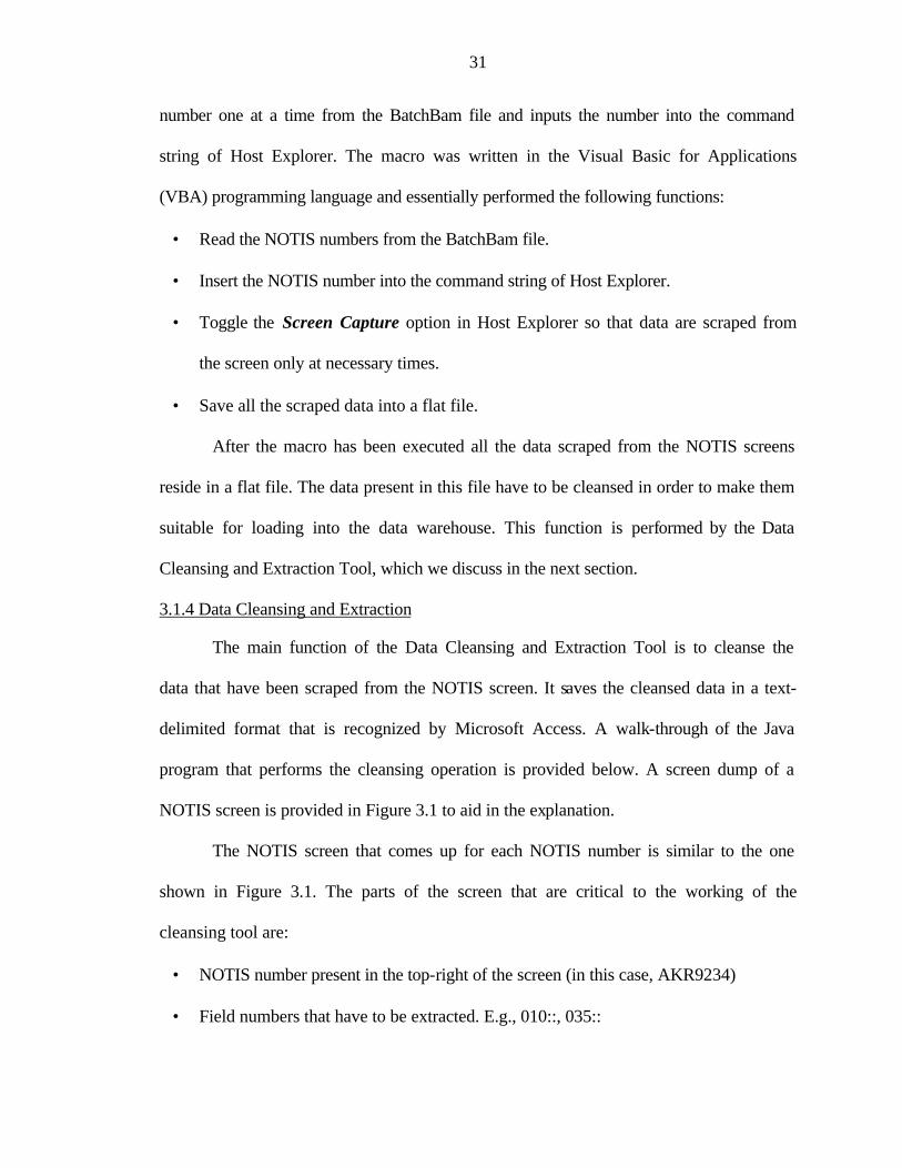
3.1.4 Data Cleansing and Extraction
The main function of the Data Cleansing and Extraction Tool is to cleanse the
data that have been scraped from the NOTIS screen. It saves the cleansed data in a text-
delimited format that is recognized by Microsoft Access. A walk-through of the Java
program that performs the cleansing operation is provided below. A screen dump of a
NOTIS screen is provided in Figure 3.1 to aid in the explanation.
The NOTIS screen that comes up for each NOTIS number is similar to the one
shown in Figure 3.1. The parts of the screen that are critical to the working of the
cleansing tool are:
• NOTIS number present in the top-right of the screen (in this case, AKR9234)
• Field numbers that have to be extracted. E.g., 010::, 035::
32
• Delimiters
The “|” symbol is used as the delimiter throughout the program. For example, in the
260 field of the bibliographic record shown in Figure 3.1 below,
“|a” delimits the place of publication,
“|b” the name of the publisher and,
“|c” the date of publication.
Figure 3.1 A Sample NOTIS Screen
We now take you on a brief walk-through of the data cleansing and extraction process.
On completion of the screen-scraping process, we have a flat file that contains all the
records that have been scraped. We also possess the BatchBam file that contains the
NOTIS numbers of the records that have been scraped. These files need to be read by the
33
Data Cleansing Tool and the necessary fields then need to be extracted. The major steps
involved in this process of cleansing and extraction are outlined below:
• The entire list of NOTIS numbers is read from the BatchBam file and stored in a
data structure.
• The flat file containing the scraped data is then parsed using the NOTIS numbers as
the delimiters. Each token that results from the parser contains a single NOTIS
record.
• Each of these records is now broken down further based on the field numbers and
only the necessary fields are retained.
• A considerable amount of the data present on the NOTIS screen is unnecessary
from the point of view of our project. As has been mentioned earlier, we need only
certain fields from the NOTIS screen. But even from these fields we need the data
only from certain delimiters. Therefore, we now scan each of the above-obtained
fields for a certain set of delimiters, which was pre-defined for each individual field.
The data present in the other delimiters are discarded.
• The data collected from the various fields and their corresponding delimiters are
then written to a flat file. Some fields contain data from more than one delimiter
concatenated together. The reason for this can be explained as follows. There are
certain fields, which are present in the database only for informational purposes and
will not be used as a criteria field in any query. Since these fields will never be
queried upon, they do not require to be cleansed as rigorously as the other fields and
therefore, we can afford to leave the data in these fields as concatenated strings.
Example: The Catalog_source field which has data from “|a” and “|c” is of the form
34
“|a DLC |c DLC” while the Lang code field which has data from “|a” and “|h” is of
the form “|a eng |h rus”. But we split this into two fields namely, Lang_code_1
containing “eng” and Lang_code_2 containing “rus”.
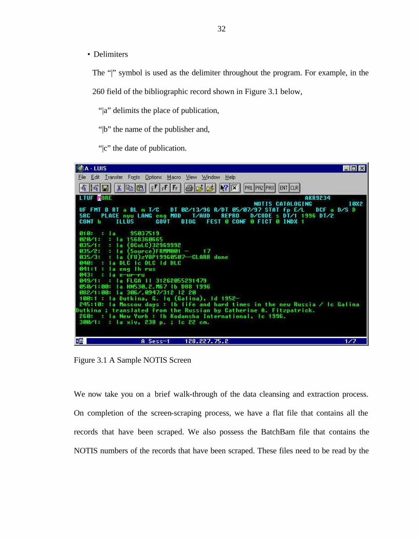
• All the data collected from the various fields are stored in a flat file in text-
delimited format. It can now be loaded into the warehouse database.
A screen dump of the text-delimited file, which is the end result of the cleansing
operations, is shown below in Figure 3.2.
Figure 3.2 A Text-Delimited File
3.1.5 Data Loading Manager
The main function of the Data Loading Manager is loading the scraped data into
the warehouse database maintained in Microsoft Access. Loading a data warehouse is
35
complex and typically involves a variety of sources, including legacy, file-based, and
relational systems. Conventional relational bulk-load and replication mechanisms cannot
perform complex data transformations, nor can they load a data warehouse fast enough.
The simple relational bulk loaders perform bulk loading as a series of steps, and they
cannot perform much processing during the data loading.
In our case, although we did have different sources for our data, the loading
manager has to deal with only one source of data, namely, text-delimited files which are
the output of the cleansing tool. We also do not need to perform any complex data
transformations. As a result, we decided to implement a very simple algorithm to perform
the loading of the data into the warehouse. Each line in the cleansed, text-delimited file
represents a single record in the database. The loading manager converts each line into an
SQL – INSERT statement and thereby loads the data in the warehouse database. The
loading manager also defines the corresponding keys for the different relations that exist
in the database.
3.2 Warehouse Run-time Tools
A decision support system is characterized by the kind of analysis tools that are
offered to the user at run-time. Decision-makers need to be allowed the flexibility to issue
a variety of queries to retrieve useful information from the warehouse. Two general types
of queries can be distinguished: pre-defined and ad hoc queries. The former refers to
queries that are frequently used by decision-makers for accessing information from
different snapshots of data imported into the warehouse. The latter refers to queries that
are exploratory in nature. A decision-maker suspects that there is some relationship
between different types of data and issues a query to verify the existence of such a

36
relationship. Alternatively, data mining tools can be applied to analyze the data contents
of the warehouse and discover rules of their relationships (or associations). In this
section, we discuss the different querying options offered by LDSS and the issues
involved with them. The data mining aspect will be discussed in a later section.
3.2.1 Canned Queries
Below are some sample queries posted in English. Their corresponding SQL
queries have been pre-defined and can be run by the user by a click of the mouse using
LDSS.
1. Number and percentage of approval titles circulated and non-circulated.
2. Number and percentage of firm order titles circulated and non-circulated.
3. Amount of financial resources spent on acquiring non-circulated titles.
4. Number and percentage of DLC/DLC cataloging records in circulated and non-
circulated titles.
5. Number and percentage of “shared” cataloging records in circulated and non-
circulated titles.
6. Numbers of original and “shared” cataloging records of non-circulated titles.
7. Identify the broad subject areas of circulated and non-circulated titles.
8. Identify titles that have been circulated “n” number of times and by subjects.
9. Number of circulated titles without the 505 field.
Each of the above English queries can be realized by a number of SQL queries.
Since canned queries are nothing but standard SQL queries that have been pre-defined,
no explanation is needed on their actual implementation. Instead, a few sample query
outputs are provided in the next section.
37
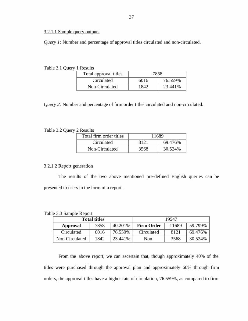
3.2.1.1 Sample query outputs
Query 1: Number and percentage of approval titles circulated and non-circulated.
Table 3.1 Query 1 Results Total approval titles 7858
Circulated 6016 76.559% Non-Circulated 1842 23.441%
Query 2: Number and percentage of firm order titles circulated and non-circulated.
Table 3.2 Query 2 Results Total firm order titles 11689
Circulated 8121 69.476% Non-Circulated 3568 30.524%
3.2.1.2 Report generation
The results of the two above mentioned pre-defined English queries can be
presented to users in the form of a report.
Table 3.3 Sample Report Total titles 19547
Approval 7858 40.201% Firm Order 11689 59.799% Circulated 6016 76.559% Circulated 8121 69.476%
Non-Circulated 1842 23.441% Non- 3568 30.524%
From the above report, we can ascertain that, though approximately 40% of the
titles were purchased through the approval plan and approximately 60% through firm
orders, the approval titles have a higher rate of circulation, 76.559%, as compared to firm
38
order titles of 69.476%. It is important to note that the result of the above queries is taken
from only one snapshot of the circulation data. Analysis from several snapshots in order
to compare the results and arrive with reliable information.
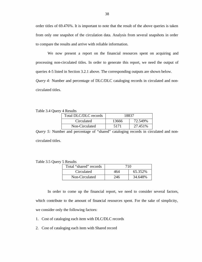
We now present a report on the financial resources spent on acquiring and
processing non-circulated titles. In order to generate this report, we need the output of
queries 4-5 listed in Section 3.2.1 above. The corresponding outputs are shown below.
Query 4: Number and percentage of DLC/DLC cataloging records in circulated and non-
circulated titles.
Table 3.4 Query 4 Results Total DLC/DLC records 18837
Circulated 13666 72.549% Non-Circulated 5171 27.451%
Query 5: Number and percentage of “shared” cataloging records in circulated and non-
circulated titles.
Table 3.5 Query 5 Results Total “shared” records 710
Circulated 464 65.352% Non-Circulated 246 34.648%
In order to come up the financial report, we need to consider several factors,
which contribute to the amount of financial resources spent. For the sake of simplicity,
we consider only the following factors:
1. Cost of cataloging each item with DLC/DLC records
2. Cost of cataloging each item with Shared record

39
3. Average price of non-circulated books
4. Average pages of non-circulated books
5. Value of shelf space per centimeter
Since the value of the above factors differs from institution to institution and
might change according to more efficient workflow and better equipment used, users are
required to fill in the value for factor 1, 2 and 5. LDSS can compute factors 3 and 4. The
financial report, taking into consideration the value of the above factors, could be as
shown below.
Processing cost of each DLC Title = $10.00
5171 x $10.00 = $ 51,710.00
Processing cost of each Shared Title = $20.00
246 x $20.00 = $ 4,920.00
Average price paid per non-circulated item = $36.00
5417 x $36.00 = $ 195,012.00
Average size of book = 300 pages = 3 cm.
Average cost of 1 cm of shelf space = $0.10
5417 x $0.30 = $ 1625.10
Grand Total = $ 253,267.10
Again it is important to point out that several snapshots of the circulation data
have to be taken to track and compare the different analysis before deriving the reliable
information.
3.2.2 Ad-Hoc Queries
Alternately, if the user wishes to issue a query that has not been pre-defined, the
Ad-Hoc Query Wizard can be used. The following example illustrates the use of the Ad-

40
Hoc Query Wizard. Assume the sample query is: How many circulated titles in the
English subject area cost more than $35.00?
We now take you on a walk-through of the Ad-Hoc Query Wizard starting from
the first step till the output is obtained.
Figure 3.3 depicts Step 1 of the Ad-Hoc Query Wizard. The sample query
mentioned above requires the following fields:
• Bib_key for a count of all the titles which satisfy the given condition.
• Charges to specify the criteria of “circulated title”.
• Fund-Key to specify all titles under the “English” subject area.
• Paid_Amt to specify all titles which cost more than $35.00.
Figure 3.3 Step 1: Ad-Hoc Query Wizard
41
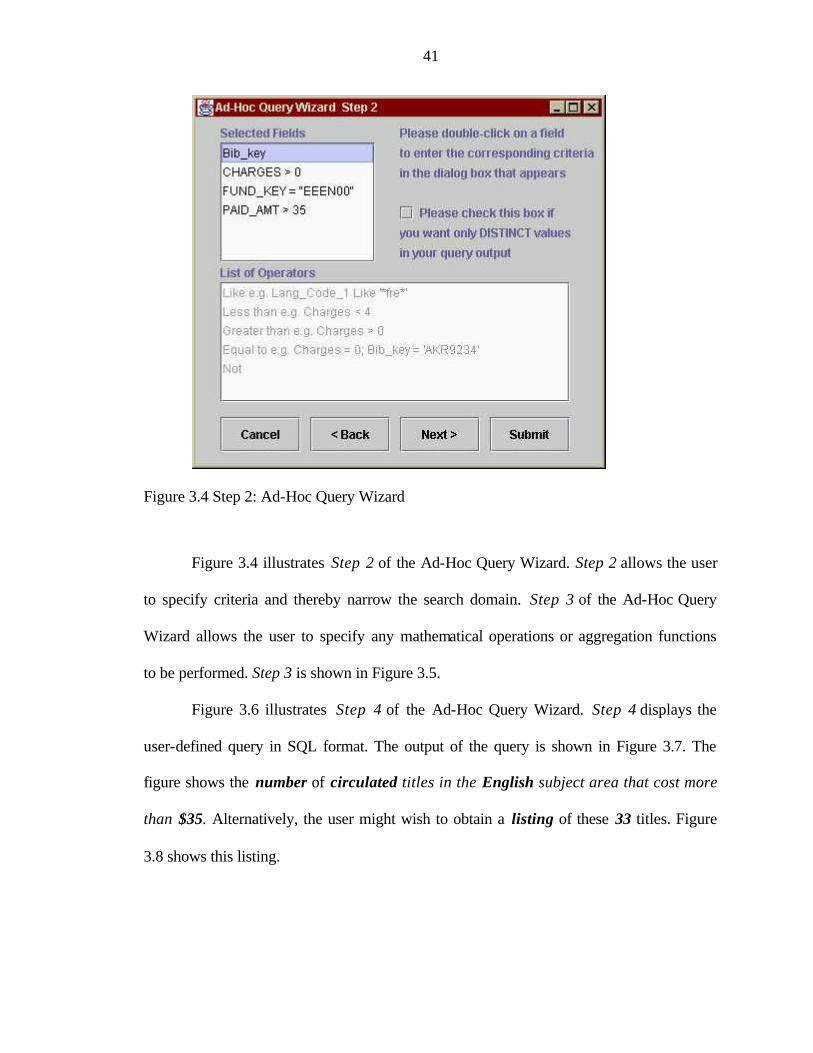
Figure 3.4 Step 2: Ad-Hoc Query Wizard
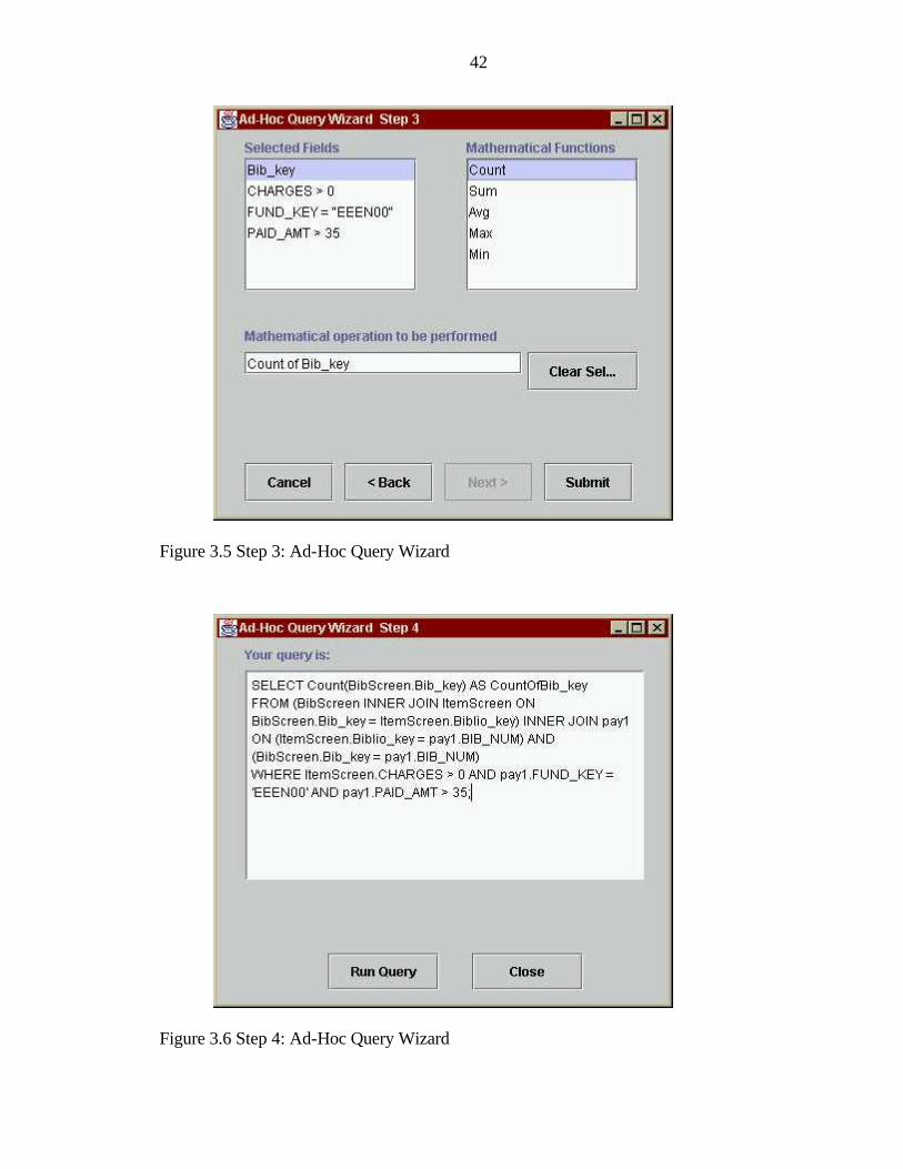
Figure 3.4 illustrates Step 2 of the Ad-Hoc Query Wizard. Step 2 allows the user
to specify criteria and thereby narrow the search domain. Step 3 of the Ad-Hoc Query
Wizard allows the user to specify any mathematical operations or aggregation functions
to be performed. Step 3 is shown in Figure 3.5.
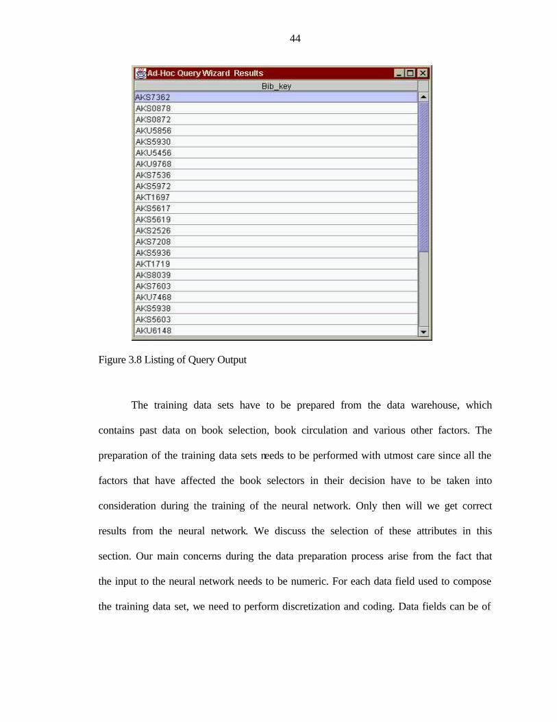
Figure 3.6 illustrates Step 4 of the Ad-Hoc Query Wizard. Step 4 displays the
user-defined query in SQL format. The output of the query is shown in Figure 3.7. The
figure shows the number of circulated titles in the English subject area that cost more
than $35. Alternatively, the user might wish to obtain a listing of these 33 titles. Figure
3.8 shows this listing.
42
Figure 3.5 Step 3: Ad-Hoc Query Wizard
Figure 3.6 Step 4: Ad-Hoc Query Wizard

43
Figure 3.7 Query Output
3.3 Data Mining Build-time Tool
In this section, we take a closer look at LibMine, the Data Mining component of
LDSS. As has been discussed earlier, LibMine performs the data mining with the aid of
DOMRUL, a neural-network model for learning domain rules. We now discuss each of
the components of LibMine in detail.
3.3.1 Data Preparation
Data preparation is the most important step involved in the entire process of data
mining. The importance of data preparation is amplified more so ever due to our use of
neural networks. A neural network model needs to be trained in order for it to make
predictions. In our case, we have to train the neural network to approximate the behavior
of the book selectors.
44
Figure 3.8 Listing of Query Output
The training data sets have to be prepared from the data warehouse, which
contains past data on book selection, book circulation and various other factors. The
preparation of the training data sets needs to be performed with utmost care since all the
factors that have affected the book selectors in their decision have to be taken into
consideration during the training of the neural network. Only then will we get correct
results from the neural network. We discuss the selection of these attributes in this
section. Our main concerns during the data preparation process arise from the fact that
the input to the neural network needs to be numeric. For each data field used to compose
the training data set, we need to perform discretization and coding. Data fields can be of
45
two types, numeric and non-numeric. Attributes need to be handled differently based on
their data type. We discuss these two different processes in this section.
3.3.1.1 Selection of non-goal attributes (feature vector)
The training data set that is submitted to DOMRUL consists of a single goal
attribute and a set of non-goal attributes. The Feature Vector represents a set of non-goal
attributes that have a bearing on the goal attribute of the particular training data set. A
feature vector is a vector where each element is a feature value. A feature here means a
non-goal attribute. In library terms, features are factors that are involved during the book
selection process. The user, in this case, the book selector, needs to select those attributes
that have been involved in his/her book selection process as the feature vector of the
training data set. It is crucial for the user to select only those features that were actually
involved in the selection process since DOMRUL uses the feature vector to learn domain
rules and the generated rules will reflect the importance of the features used to compose
the training data set. If a meaningless attribute is chosen to be part of the feature vector in
the composition of a training data set, the generated rules will reflect this fact.
3.3.1.2 Discretization of continuous attributes
Discretization is performed by dividing the values of a numeric (continuous)
attribute into a small number of intervals, where each interval is mapped to a discrete
(categorical, nominal, symbolic) symbol. The discretization algorithm employed by
LDSS is an extension of the C4.525 algorithm. The C4.5 algorithm is a member of the
ID3 family of decision tree algorithms. In C4.5 the same measure used to choose the best
attribute to branch on at each node of the decision tree is used to determine the best value
for splitting a numeric attribute into two intervals. This value, called a cutpoint, is found
by exhaustively checking all possible binary splits of the current interval and choosing
46
the splitting value that maximizes the information gain measure. We have a set of records
obtained from the data warehouse. Each record has the same structure, consisting of a
number of attribute/value pairs. One of these attributes represents the goal of the record,
i.e. the attribute whose values are most significant to us. In our case, the goal attribute
would specify if the book represented by the record was selected or not. The problem is
to build a decision tree that on the basis of answers to questions about the non-goal
attributes predicts correctly the value of the goal attribute. In our case, the goal attribute
takes the values of {success, failure}. The basic ideas behind the algorithm used are that:
• In the decision tree, each node corresponds to a non-goal attribute and each arc to a
possible value of that attribute. A leaf of the tree specifies the expected value of the
goal attribute for the records described by the path from the root to that leaf.
• In the decision tree, at each node should be associated the non-goal attribute which
is most informative among the attributes not yet considered in the path from the
root.
• Entropy is used to measure how informative a node is.
We now proceed to provide a few definitions of the various terms used. But prior
to that, we provide a sample data set to aid in the explanation of the discretization
algorithm. In the examples that accompany the definitions, the following assumptions
have been made. The examples are valid only for a particular set of cutpoints. The
discretization algorithm employed by LDSS exhaustively checks all split points.
• Number of clusters = 3 (Low, Medium and High)
• “Cutpoints” are as follows: (Charges � 1 ⇒ Low, 2 � Charges � 4 ⇒ Medium,
Charges > 4⇒ High)
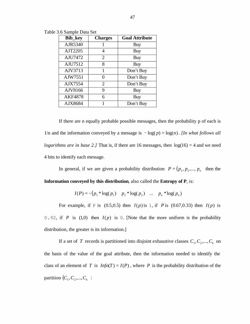
47
Table 3.6 Sample Data Set Bib_key Charges Goal Attribute AJR5340 1 Buy AJT2205 4 Buy AJU7472 2 Buy AJU7512 8 Buy AJV3713 1 Don’t Buy AJW7551 0 Don’t Buy AJX7554 2 Don’t Buy AJV8166 9 Buy AKF4878 6 Buy AJX8684 1 Don’t Buy
If there are n equally probable possible messages, then the probability p of each is
1/n and the information conveyed by a message is )log()log( np =− . [In what follows all
logarithms are in base 2.] That is, if there are 16 messages, then 4)16log( = and we need
4 bits to identify each message.
In general, if we are given a probability distribution ( )npppP ,...,, 21= then the
Information conveyed by this distribution, also called the Entropy of P, is:
( ))log(*...)log(*)log(*)( 2211 nn ppppppPI +++−=
For example, if P is )5.0,5.0( then )(pI is 1, if P is )33.0,67.0( then )(pI is
0.92, if P is )0,1( then )(pI is 0. [Note that the more uniform is the probability
distribution, the greater is its information.]
If a set of T records is partitioned into disjoint exhaustive classes kCCC ,...,, 21 on
the basis of the value of the goal attribute, then the information needed to identify the
class of an element of T is )()( PITInfo = , where P is the probability distribution of the
partition ( )kCCC ,...,, 21 :
48
=
T
C
T
C
T
CP k,...,, 21
In the case of the sample data set provided in Table 6, we have
( ) ( ) 97.0104,106 == ITInfo (constant for a given training data set)
If we first partition T on the basis of the value of a non-goal attribute X into sets
nTTT ,...,, 21 then the information needed to identify the class of an element of T becomes
the weighted average of the information needed to identify the class of an element of iT ,
i.e. the weighted average of ( )iTInfo :
( ) ( )i
n
i
i TInfoT
TTXInfo *
||
||,
1∑
=
=
In the case of the sample data set provided in Table 6, for the attribute “Charges”,
we have
( ) ( ) ( ) ( )0,33*10331,32*10343,41*104,arg IIITesChInfo ++=
( ) 6.0,arg =∴ TesChInfo
Consider the quantity ( )TXGain , defined as
( ) ( ) ( )TXInfoTInfoTXGain ,, −=
This represents the difference between the information needed to identify an
element of T and the information needed to identify an element of T after the value of
attribute X has been obtained, that is, this is the gain in information due to attribute X .
In the case of the sample data set provided in Table 6, for the attribute Charges,
the gain is
( ) ( ) ( ) 37.06.097.0,arg,arg =−=−= TesChInfoTInfoTesChGain
49
This notion of Gain tends to favor attributes that have a large number of values.
For example, if we have an attribute D that has a distinct value for each record, then
( )TDInfo , is 0, thus ( )TDGain , is maximal. To compensate for this Quinlan suggests
using the following ratio instead of Gain:
( ) ( )( )TDSplitInfo
TDGainTDGainRatio
,
,, =
where ( )TDSplitInfo , is the information due to the split of T on the basis
of the value of the goal attribute D . Thus ( )TDSplitInfo , is
T
T
T
T
T
TI m,...,, 21
where { }mTTT ,...,, 21 is the partition of T induced by the values of D .
In the case of the sample data set provided in Table 6, for the attribute Charges,
we have
( ) ( ) ( ) ( )103log*103103log*103104log*104,arg −−−=TesChSplitInfo
( ) 571.1,arg =∴ TesChSplitInfo
( ) 236.0571.137.0,arg ==∴ TesChGainRatio
The examples provided are for a particular case, which was mentioned previously.
The LDSS discretization algorithm explores all possible combinations of split points
before arriving upon the optimal cutpoints, which maximize gain ratio.
Although the discretization manager automatically chooses the intervals
efficiently and discretizes the data from the warehouse to fit these intervals, there exist
certain limitations. In the present version of the LDSS, a continuous attribute can be
discretized only into three intervals. But the modification of this feature to support any
number of intervals is trivial and can be treated as future work.

50
3.3.1.3 Grouping similar non-numeric attribute values
So far we discussed the issues involved with numeric attributes. But non-numeric
attributes present entirely new problems. In this section we discuss the issues involved
with preparing non-numeric attributes for data mining.
To be used in a neural network, values for non-numeric fields such as Publisher,
Author or Language need to be coded and mapped into “new fields”, taking the values 0
or 1. This means that the attribute Publisher that may have the 5 values {Addison-
Wesley, Longman, McGraw-Hill, Oxford, Cambridge} is broken into 5 new fields, called
Addison-Wesley, Longman, McGraw-Hill, Oxford, Cambridge each taking the value 0 or
1, depending on the value in the record. For each record, only one of these fields has the
value 1, and the others have the value 0.
Consider the sample data set of the attribute Publisher shown below. It is fairly
obvious that the records {AKR9234, AKS4728, AJX7554, ARP6734, APT3298} have
the same publisher. But due to inconsistent abbreviations and discrepancy in punctuation,
the fact that these records have the same publisher is not reflected in the training data set.
This needs to be corrected.
The correction for this problem could have been performed earlier during the
cleansing operation prior to loading the data into the warehouse database. But since the
cleansing operation was already cumbersome and slow, we decided to skip this correction
and instead, perform it before preparing the training data set.
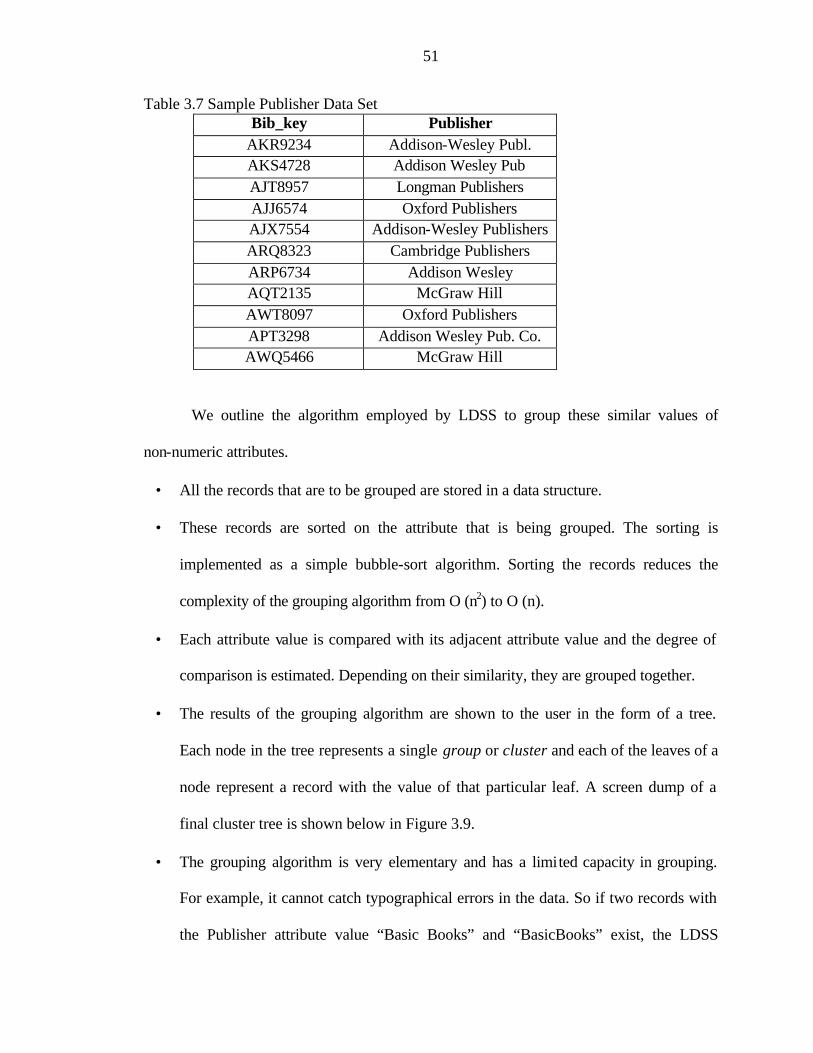
51
Table 3.7 Sample Publisher Data Set Bib_key Publisher
AKR9234 Addison-Wesley Publ. AKS4728 Addison Wesley Pub AJT8957 Longman Publishers AJJ6574 Oxford Publishers AJX7554 Addison-Wesley Publishers ARQ8323 Cambridge Publishers ARP6734 Addison Wesley AQT2135 McGraw Hill AWT8097 Oxford Publishers APT3298 Addison Wesley Pub. Co. AWQ5466 McGraw Hill
We outline the algorithm employed by LDSS to group these similar values of
non-numeric attributes.
• All the records that are to be grouped are stored in a data structure.
• These records are sorted on the attribute that is being grouped. The sorting is
implemented as a simple bubble-sort algorithm. Sorting the records reduces the
complexity of the grouping algorithm from O (n2) to O (n).
• Each attribute value is compared with its adjacent attribute value and the degree of
comparison is estimated. Depending on their similarity, they are grouped together.
• The results of the grouping algorithm are shown to the user in the form of a tree.
Each node in the tree represents a single group or cluster and each of the leaves of a
node represent a record with the value of that particular leaf. A screen dump of a
final cluster tree is shown below in Figure 3.9.
• The grouping algorithm is very elementary and has a limited capacity in grouping.
For example, it cannot catch typographical errors in the data. So if two records with
the Publisher attribute value “Basic Books” and “BasicBooks” exist, the LDSS
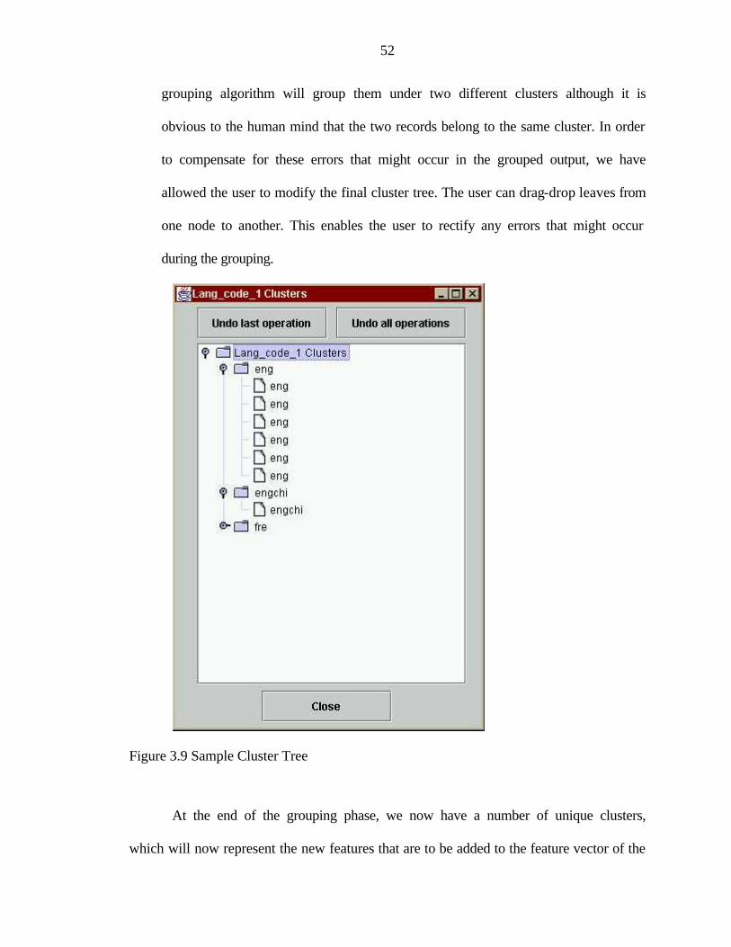
52
grouping algorithm will group them under two different clusters although it is
obvious to the human mind that the two records belong to the same cluster. In order
to compensate for these errors that might occur in the grouped output, we have
allowed the user to modify the final cluster tree. The user can drag-drop leaves from
one node to another. This enables the user to rectify any errors that might occur
during the grouping.
Figure 3.9 Sample Cluster Tree
At the end of the grouping phase, we now have a number of unique clusters,
which will now represent the new features that are to be added to the feature vector of the
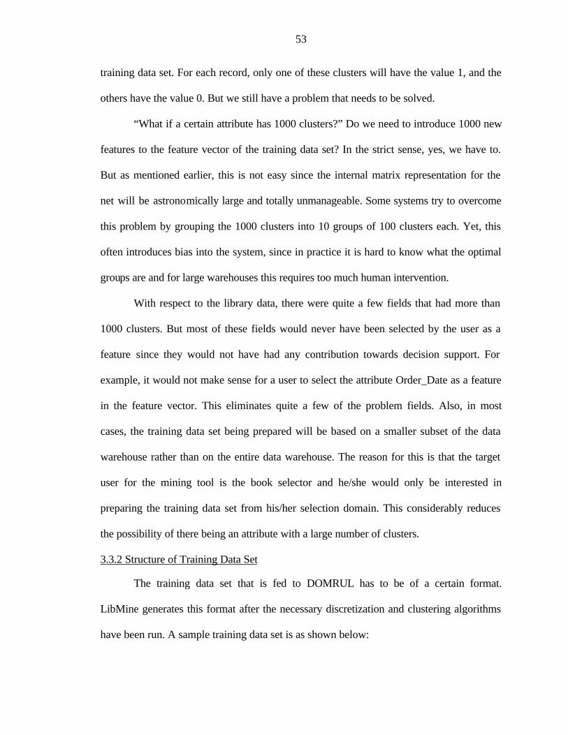
53
training data set. For each record, only one of these clusters will have the value 1, and the
others have the value 0. But we still have a problem that needs to be solved.
“What if a certain attribute has 1000 clusters?” Do we need to introduce 1000 new
features to the feature vector of the training data set? In the strict sense, yes, we have to.
But as mentioned earlier, this is not easy since the internal matrix representation for the
net will be astronomically large and totally unmanageable. Some systems try to overcome
this problem by grouping the 1000 clusters into 10 groups of 100 clusters each. Yet, this
often introduces bias into the system, since in practice it is hard to know what the optimal
groups are and for large warehouses this requires too much human intervention.
With respect to the library data, there were quite a few fields that had more than
1000 clusters. But most of these fields would never have been selected by the user as a
feature since they would not have had any contribution towards decision support. For
example, it would not make sense for a user to select the attribute Order_Date as a feature
in the feature vector. This eliminates quite a few of the problem fields. Also, in most
cases, the training data set being prepared will be based on a smaller subset of the data
warehouse rather than on the entire data warehouse. The reason for this is that the target
user for the mining tool is the book selector and he/she would only be interested in
preparing the training data set from his/her selection domain. This considerably reduces
the possibility of there being an attribute with a large number of clusters.
3.3.2 Structure of Training Data Set
The training data set that is fed to DOMRUL has to be of a certain format.
LibMine generates this format after the necessary discretization and clustering algorithms
have been run. A sample training data set is as shown below:
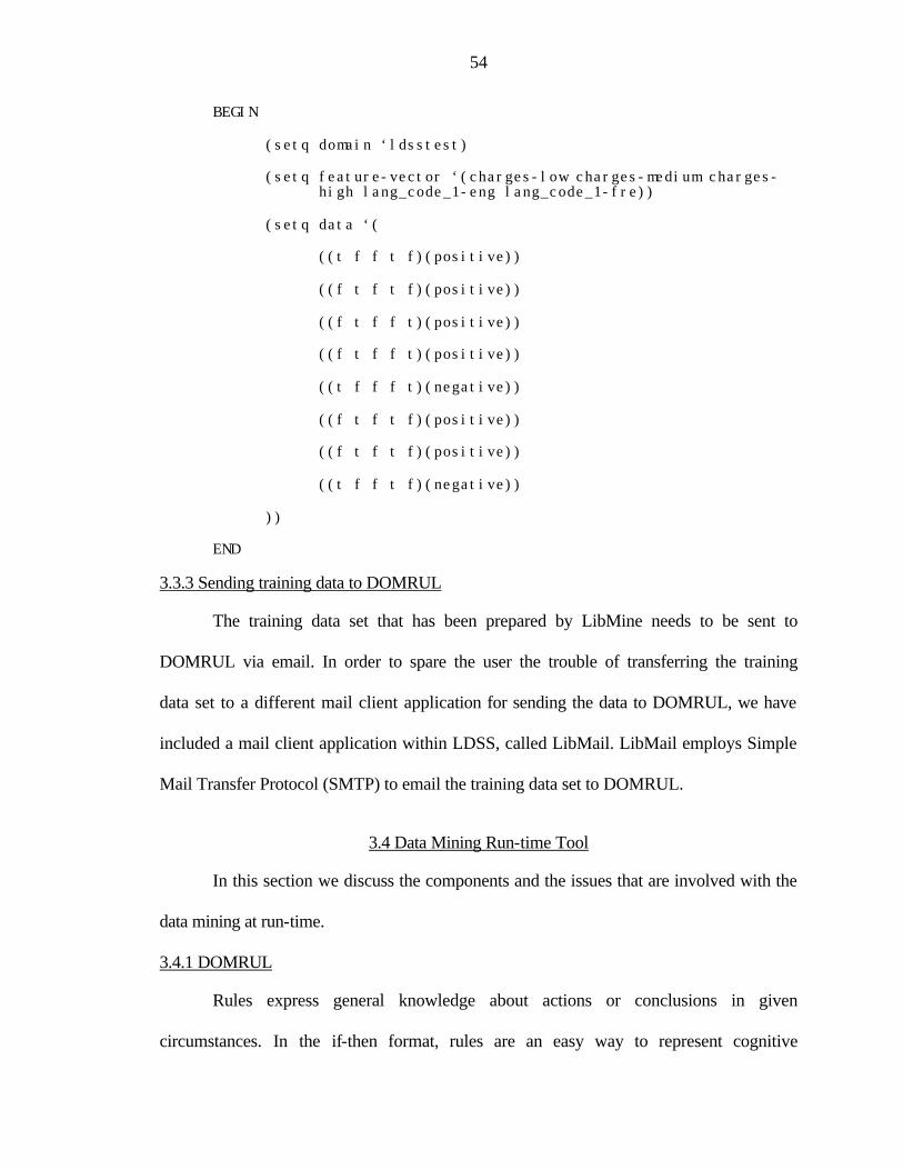
54
BEGIN
(setq domain ‘ldsstest)
(setq feature-vector ‘(charges-low charges-medium charges-high lang_code_1-eng lang_code_1-fre))
(setq data ‘(
((t f f t f)(positive))
((f t f t f)(positive))
((f t f f t)(positive))
((f t f f t)(positive))
((t f f f t)(negative))
((f t f t f)(positive))
((f t f t f)(positive))
((t f f t f)(negative))
))
END
3.3.3 Sending training data to DOMRUL
The training data set that has been prepared by LibMine needs to be sent to
DOMRUL via email. In order to spare the user the trouble of transferring the training
data set to a different mail client application for sending the data to DOMRUL, we have
included a mail client application within LDSS, called LibMail. LibMail employs Simple
Mail Transfer Protocol (SMTP) to email the training data set to DOMRUL.
3.4 Data Mining Run-time Tool
In this section we discuss the components and the issues that are involved with the
data mining at run-time.
3.4.1 DOMRUL
Rules express general knowledge about actions or conclusions in given
circumstances. In the if-then format, rules are an easy way to represent cognitive

55
processes in psychology and a useful means to encode expert knowledge in expert
systems26. There are several alternatives for rule learning. In symbolic artificial
intelligence, learning is often viewed as a search in a defined hypothesis space. C4.525 is
a popular rule-learning tool based on the decision-tree approach. This approach, however,
does not conduct multivariate search for rules. In logic, rule learning is called inductive
logic programming27, e.g., an approach based on inverting the deductive operators of
theorem provers. The logic approach, however, does not handle the nature of uncertainty.
Recently, the neural-network approach emerges as promising because it deals with both
multivariate search and the issue of uncertainty. The traditional disadvantage with this
approach is, however, that the neural-network knowledge is cryptically coded as a large
number of weights and their semantics in terms of the problem to be solved is not
explicit.
There are two general approaches to extracting symbolic knowledge from a
trained neural network. In one approach, each internal element in the neural network is
examined whereas in another, only the input-output behavior is observed. The first
approach is an open-box approach, also called the decompositional approach. The second
approach is a black-box approach, sometimes called the pedagogical approach. In
general, the open-box approach is more analytical whereas the black-box is more
empirical in nature. A recent survey of this topic can be found in Survey and critique of
techniques for extracting rules from trained artificial neural networks28.
The task of rule learning is to learn or discover a set of rules from given instances
called training instances. Ideally, the learned rules as a whole should explain not just the
training instances but also unseen instances in the domain. This addresses an important

56
issue, namely, generalization, which forms the basis of evaluating the performance of a
learning system. A challenging criterion for judging the success of a learning system is
based on whether it can identify the domain rules exactly rather than how well it can
generalize. Here, the domain rules refer to the set of rules, which can explain all the
domain instances. If such rules are learned, generalization error should be zero. In
addition, the domain rules provide insight into the precise nature of the domain.
An in-depth discussion of DOMRUL24, rule learning and rule extraction can be
found in A Neural-Network Model for Learning Domain Rules Based on Its Activation
Function Characteristics29.
3.4.2 Results of test runs
We composed a number of training data sets and submitted them to DOMRUL in
order to test the data-mining component of LDSS. These training data sets were
composed with great care after interviewing three different book selectors at the
University of Florida Library in order to obtain their input as to the features that are
involved in their book selection process. The test results shown in this section only
belong to the selection domain of two different book selectors because two of the three
book selectors provided the same set of features. An explanation of the generated rules
and their corresponding feature vector is provided below.
Result 1 has been obtained using the selection criteria of Betsy Simpson who is a
book selector at the University of Florida Library. As can be seen, the two attributes that
have been used as features in the feature vector are Publisher and Charges. The attribute
Publisher represents the Publisher of the particular record or book and the attribute
Charges represents the number of times the particular book has been checked out by a
library patron. The attribute Publisher has been grouped into six different categories from

57
Category A to Category F ranging from the lowest to the highest priority. So, publishers
under Category F are most likely to have their books selected solely because of their
reputation in the given field. The attribute Charges has been discretized into three
intervals, namely, low, medium and high.
Result 1 has been obtained using the selection criteria of Betsy Simpson who is a
book selector at the University of Florida Library. As can be seen, the two attributes that
have been used as features in the feature vectors are Publisher and Charges. The attribute
Publisher represents the Publisher of the corresponding book and the attribute Charges
represents the number of times the particular book has been checked out by a library
patron.
Result 1
The Domain: Betsy Simpson’s Selection Criteria without Paid_Amt
The Feature Vector: (PUBLISHER-CATEGORYA PUBLISHER-CATEGORYB PUBLISHER-
CATEGORYC PUBLISHER-CATEGORYD PUBLISHER-CATEGORYE PUBLISHER-CATEGORYF
CHARGES-LOW CHARGES-MEDIUM CHARGES-HIGH)
The Rules:
IF (PUBLISHER-CATEGORYD) and CHARGES-LOW THEN it is a positive instance (confidence level = High) IF (NOT PUBLISHER-CATEGORYE) and CHARGES-LOW THEN it is a positive instance (confidence level = High)
As can be seen, two rules have been generated with this training data set. These rules can
be read in the following manner for better understanding.

58
1. If the publisher of the book belongs to Category D, the book is still worth buying
even though it will be checked out only very few times.
2. If the publisher of the book does not belong to Category E, the book is still worth
buying even though it will be checked out only very few times.
The above rules might appear cryptic in nature because one usually associates the number
of times a book has been checked out to its popularity or worthiness. So, one might feel
that a book that has been checked out very few times, cannot be deemed to have been
worth buying. But at the University of Florida Library, books are often bought or ordered
for many reasons that are not associated with the attribute Charges. For example, a
certain faculty member might require a book for research purposes and as a result, that
particular book might have a very low value in the Charges column. But the University of
Florida Library still considers that particular book to be worth buying. Factors such as
these are not maintained in the warehouse database and there was no way to compensate
for their absence while composing the training data set. As a result, the above rules need
to be interpreted with the understanding that many such factors were not included in the
feature vector of the training data set. Although the above rules may not make particular
sense to the common reader, they do provide important information to the selectors at the
University of Florida Library.
Result 2 was obtained using the selection criteria of Blake Landor who is also a
book selector at the University of Florida Library. As can be seen, the two attributes that
have been used as features in the feature vector are Publisher and Paid_Amt. The
explanation of the attribute Publisher has been provided with Result 1. The attribute
Paid_Amt represents the cost of the particular book. The attribute Publisher has been
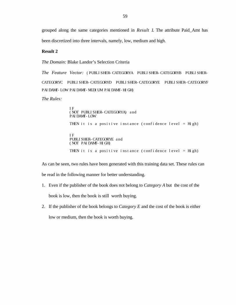
59
grouped along the same categories mentioned in Result 1. The attribute Paid_Amt has
been discretized into three intervals, namely, low, medium and high.
Result 2
The Domain: Blake Landor’s Selection Criteria
The Feature Vector: (PUBLISHER-CATEGORYA PUBLISHER-CATEGORYB PUBLISHER-
CATEGORYC PUBLISHER-CATEGORYD PUBLISHER-CATEGORYE PUBLISHER-CATEGORYF
PAIDAMT-LOW PAIDAMT-MEDIUM PAIDAMT-HIGH)
The Rules:
IF (NOT PUBLISHER-CATEGORYA) and PAIDAMT-LOW THEN it is a positive instance (confidence level = High) IF PUBLISHER-CATEGORYE and (NOT PAIDAMT-HIGH) THEN it is a positive instance (confidence level = High)
As can be seen, two rules have been generated with this training data set. These rules can
be read in the following manner for better understanding.
1. Even if the publisher of the book does not belong to Category A but the cost of the
book is low, then the book is still worth buying.
2. If the publisher of the book belongs to Category E and the cost of the book is either
low or medium, then the book is worth buying.
60
CHAPTER 4 SUMMARY AND CONCLUSIONS
This thesis describes the design and implementation of a Library Decision
Support System (LDSS). We described the functions of the different components of
LDSS. The screen scraping and data cleansing and extraction processes were described in
detail. The process of importing data stored in LUIS as separate data files into the
warehouse database was also described. The data contents of the warehouse can provide a
very rich information source to aid the library management in decision making. Using the
implemented system, a decision-maker can use the GUI to establish the warehouse, and
activate the querying facilities provided by LDSS, to explore the warehouse contents.
Many types of queries can be formulated and issued against the warehouse database.
Experimental results indicate that the querying tools are very effective and provide
pertinent information for aiding the library management in making decisions. We also
described the data mining component (LibMine) present in LDSS. LibMine can be used
to compose a training data set from the data present in the warehouse database.
Discretization and clustering algorithms, which are essential during this process of
composing the training data set, were described in detail. The composed training data set
is then submitted to the neural network, DOMRUL. The basics of DOMRUL were
described and a pointer to detailed information on DOMRUL was provided. The
developed prototype system and its tools can potentially be applied to the analysis and
rule discovery of many other types of data in support of library management.
61
A decision support system gives targeted decision-makers the user-friendly, clear
view of their business. The decision-makers are described as “targeted” because the
system needs to have been developed, taking into consideration their goals and
information requirements. These decision-makers use similar terms and definitions to
describe their business and have similar goals. In our case, the library management and
book selectors form the set of decision-makers. One of their common goals is the
efficient expenditure of the library budget. LDSS aids them in making decisions towards
this goal.
This work stresses the importance of data warehousing and data mining
technologies in building decision support systems. Top-level library management can use
the querying tools present in LDSS to perform financial analysis and thereby, make the
expenditure of the library budget efficient. Book selectors can use the mining component
of LDSS to generate domain rules and thereby, predict whether a particular book will be
worth buying or not.
62
LIST OF REFERENCES
[1] Boorstin, D.J., “The Age of Negative Discovery,” Cleopatra’s Nose: Essays on the Unexpected, Random House, New York, 1994.
[2] Information on the ARROW system,
http://www.fcla.edu/system/intro_arrow.html [3] Strawn, G., “BatchBAMing,”
http://web.uflib.ufl.edu/rs/rsd/batchbam.html [4] Kimball, R. “Mastering Data Extraction,” DBMS Magazine, June 1996. [5] Barquin, R., Edelstein, H., eds., Planning and Designing the Data
Warehouse, Prentice Hall, Upper Saddle River, NJ, 1996. [6] Bischoff, J., Alexander, T., Data Warehouse: Practical Advice from the
Experts, Prentice Hall, Englewood Cliffs, NJ, 1997. [7] Byard, J., Schneider, D., “The Ins and Outs (and Everything in Between)
of Data Warehousing,” ACM SIGMOD 1996 Tutorial Notes, May 1996, http://www.redbrick.com/products/white/pdf/sigmod96.pdf
[8] Chaudhuri, S., Dayal, U., “An Overview of Data Warehousing and OLAP
Technology,” ACM SIGMOD Record, Vol. 26, No. 1, March 1997, http://www.acm.org/sigmod/record/issues/9703/chaudhuri.ps
[9] Devlin, B., Data Warehouse: From Architecture to Implementation, The
MIT Press, Reading, MA, 1996. [10] Hammer, J., “Data Warehousing Overview, Terminology, and Research
Issues,” http://www.cise.ufl.edu/~jhammer/classes/wh-seminar/Overview/index.htm
[11] Inmon, W.H., Building the Data Warehouse, John Wiley & Sons, Inc.,
New York, 1996. [12] Kimball, R., “Dangerous Preconceptions,” DBMS Magazine, August
1996.
63
[13] Kimball, R., The Data Warehouse Toolkit, John Wiley & Sons, Inc., New York, 1996.
[14] Barquin, R., Edelstein, H., eds., Building, Using, and Managing the Data
Warehouse, Prentice Hall, Englewood Cliffs, NJ, 1997. [15] Mendelzon, A., “Bibliography on Data Warehousing and OLAP,”
http://www.cs.toronto.edu/~mendel/dwbib.html/ [16] Symons, V., “Three Tiered Data Warehousing Structure: What it is and
How it can Benefit your Business Intelligence Implementation,” DM Review Magazine White Paper Library, June 1999.
[17] Ballard, C., Herreman, D., Schau, D., Bell, R., Kim, E., Valencic, A., Data
Modeling Techniques for Data Warehousing, SG24-2238-00, IBM Redbook, February 1998, http://www.redbooks.ibm.com/pubs/pdfs/redbooks/sg242238.pdf
[18] Ruth, D., Data Mining: An Introduction, Queens University, Belfast,
December 1995. [19] Fayyad, U., Piatetsky-Shapiro, G., Smyth, P., Uthurusamy, R., Advances
in Knowledge Discovery and Data Mining, The MIT Press, Cambridge, MA, 1996.
[20] “A New Generation of Data Mining Technologies,” An Angoss Software
Corporation White Paper, Surrey, UK, 1997. [21] “A Characterization of Data Mining Technologies and Processes,” An
Information Discovery, Inc. White Paper, Hermosa Beach, CA, 1998. [22] Okell, J., “Neural Networks versus CHAID,” smartFOCUS White Paper,
Warwick, UK, June 1999. [23] Kerber, R., “ChiMerge: Discretization of Numeric Attributes,” American
Association for Artificial Intelligence: Proceedings of the Tenth National Conference on Artificial Intelligence, pages 123-128, San Jose, CA, July 1992. AAAI Press / MIT Press, Cambridge, MA.
[24] Fu, L.M., “DOMRUL: Learning the Domain Rules,”
http://www.cise.ufl.edu/~fu/domrul.html [25] Quinlan, J.R., C4.5: Programs for Machine Learning, Morgan Kaufmann,
San Mateo, CA, 1993.

64
[26] Buchanan, B.G., Shortliffe, E.H., Eds., Rule-Based Expert Systems, Addison-Wesley, Reading, MA, 1984.
[27] Mitchell, T., Machine Learning, McGraw-Hill, New York, 1997. [28] Andrews, R., Diederich, J., Tickle, A.B., “Survey and critique of
techniques for extracting rules from trained artificial neural networks,” Knowledge-Based Syst., Vol. 8, No. 6, pages 373-389, 1995.
[29] Fu, L.M., “A Neural-Network Model for Learning Domain Rules Based
on Its Activation Function Characteristics,” IEEE Transactions on Neural Networks, Vol. 9, No. 5, pages 787-795, September 1998.

65
BIOGRAPHICAL SKETCH
Ashwin Needamangala was born on April 24, 1976, in Madras, India. He received
his Bachelor of Engineering degree from Bangalore University, Bangalore, in August
1997, majoring in electronics and communication engineering.
He joined the University of Florida in August 1998 to pursue a master’s degree in
electrical and computer engineering. He worked as a research assistant during his
master’s studies at the Database Systems Research and Development Center.
His research interests include data warehousing and data mining.