A large public dataset of annotated clinical MRIs ofpatients with acute stroke and linked metadataChin-Fu Liu 

Jonhs Hopkins UnoversityRichard Leigh 

Johns Hopkins UniversityBrenda Johnson 

Johns Hopkins UniversityVictor Urrutia 

Johns Hopkins UniversityJohnny Hsu 

Johns Hopkins UniversityXin Xu 

Johns Hopkins UniversityXin Li 

Johns Hopkins UniversitySusumu Mori 

Johns Hopkins UniversityArgye Hillis 

Johns Hopkins UniversityAndreia Faria  ( afaria1@jhmi.edu )

Johns Hopkins University

Research Article

Keywords: stroke, dataset, MRI, arti�cial intelligence, medical image, brain

Posted Date: May 31st, 2022

DOI: https://doi.org/10.21203/rs.3.rs-1705779/v1

License: This work is licensed under a Creative Commons Attribution 4.0 International License.  Read Full License

A large public dataset of annotated clinical MRIs of

patients with acute stroke and linked metadata

Chin-Fu Liu1,2, Richard Leigh3, Brenda Johnson3, Victor Urrutia3, Johnny Hsu4, Xin Xu4,

Xin Li4, Susumu Mori4, Argye E. Hillis3,5, and Andreia V. Faria4,*

1Center for Imaging Science, Johns Hopkins University, Baltimore, MD, USA

2Department of Biomedical Engineering, Johns Hopkins University, Baltimore, MD, USA

3Department of Neurology, School of Medicine, Johns Hopkins University, Baltimore, MD, USA

4Department of Radiology, School of Medicine, Johns Hopkins University, Baltimore, MD, USA

5Department of Physical Medicine & Rehabilitation, and Department of Cognitive Science, Johns Hopkins

University, Baltimore, MD, USA

*Corresponding author: afaria1@jhmi.edu

ABSTRACT

To extract meaningful and reproducible models of brain function from stroke images, for both clinical and

research proposes, is a daunting task severely hindered by the great variability of lesion frequency and

patterns. Large datasets are therefore imperative, as well as fully automated image post-processing

tools to analyze them. The development of such tools, particularly with artificial intelligence, is highly

dependent on the availability of large datasets to model training and testing. We present a public

dataset of 2,888 multimodal clinical MRIs of patients with acute and early subacute stroke, with manual

lesion segmentation, and metadata. The dataset provides high quality, large scale, human-supervised

knowledge to feed artificial intelligence models and enable further development of tools to automate

several tasks that currently rely on human labor, such as lesion segmentation, labeling, calculation of

disease-relevant scores, and lesion-based studies relating function to frequency lesion maps.

1

1 INTRODUCTION

Stroke is the 5th more frequent cause of death and a leading cause of long-term disability in the

United States1. Extracting meaningful and reproducible models of brain function from stroke images is a

daunting task severely hindered by the great variability of lesion frequency and patterns. A corollary to

this problem is that large datasets are imperative to encompass the possible lesion-function relationships.

While biomedicine has seen a shift from “anecdotal” experiences to objective, data-supported evidence

based on large amounts of data, many lesion-based studies failed to weather this transition, as evidenced

by a plethora of underpowered designs leading to inexact extrapolations, or to conclusions that cannot

be validated on external populations2–6. In addition, technical developments with artificial intelligence

(AI) depend on the availability of high quality, large scale, human-supervised dataset to generate and test

meaningful and reproducible models7–9.

A public dataset of acute stroke MRIs, associated with lesion delineation and organized non-image

information will potentially enable clinical researchers to advance in clinical modeling and prediction. It

will also enable the bioengineering community to develop and test AI algorithms of technical and clinical

relevance, e.g., for lesion segmentation, brain mapping, and automatic generation of labels and scores.

AI applications in various diseases, such as in chest X-ray, dermatology and histopathology images, and

detection of breast cancer in mammography, have drastically increased, due to the availability of large

image datasets10–15. Brain MRIs, particularly in acute conditions, offer extra challenges to the organization

of large datasets, such as the lack of data (MRI scan is costly, therefore less common), the large variability

among scanners and protocols, and the volumetric nature of the data which hinders annotation and expert

labeling. As of today, the most successful example of an open-source collection of annotated MRIs

is probably the brain tumor dataset of 750 patients included in the Medical Segmentation Decathlon

(MSD)16, used in the Brain Tumor Image Segmentation (BraTS) challenge. In acute stroke, the lack of

such large, annotated, high quality dataset, rather than mathematical or computational resources, is the

current bottleneck for AI development.

The first efforts to create stroke repositories started with population-based epidemiological studies17, 18

and did not include images. Starting in the 2,000’s, both the medical and the bioengineering communities

2/34

acknowledged the need for a central repository for acute stroke images, in addition to metadata. Initiatives

such as the “Acute Stroke Imaging Research Roadmap”19 initiated such effort, with the goal of standardiz-

ing imaging techniques, accessing the accuracy and clinical utility of imaging markers, and validating

imaging biomarkers relevant to clinical outcomes. Since then, various consortiums and trials20–25 were

able to accumulate large amounts of data, often available “after competition” and/or “upon request”.

These conditions, however, do not guarantee that the data are shared under ’FAIR’ principles26, 27, without

secondary agreements, on a timely basis, with consistent description and/or processing, and with expert

annotation. In fact, it does not even guarantee access to the raw images. A search in generalist repositories

(e.g., Dataverse, Mendeley Data, Dryad, Open Science Framework, Vivli) or using tools suited to find

“open data” (e.g., Google Dataset Search, Data Citation Index, Data.gov) mostly reveals end-analysis data

that do not serve purposes such as technical development. In addition, datasets from technical challenges

(e.g., ISLE28) or published studies usually involve a modest number of subjects and are research-focused,

acquired with homogeneous and particular protocols that do not reflect the noise and variability of clinical

data, hindering the translational potential.

We share the first annotated large dataset of clinical acute stroke MRIs, associated to demographic

and clinical metadata. Recently, a dataset of chronic stroke lesions annotated in high resolution T1-WIs

(ATLAS29) under the ENIGMA Stroke Recovery initiative30 was well received by the neuroscience and

bioengineering communities. The ATLAS has been used to improve lesion segmentation of chronic lesions

in high resolution images, to create new tools for processing chronic stroke MRIs, as well as for education

proposes31–33. Acute stroke MRIs, however, require specialized processing because of the particular lesion

intensity characteristics, the images low-resolution, heterogeneity, and noise. An analogous dataset of

acute strokes is, therefore, highly anticipated.

The resource we present consists of 2,888 clinical MRIs of patients admitted with acute or early

subacute stroke. It includes diverse protocols and MRI modalities, with typical clinical resolution. The

large sample, as well as the technical and population heterogeneity, improve the potential generalization

of models developed with these data. It includes diverse metadata, comprised of demographic information,

basic clinical profile (including National Institutes of Health Stroke Scale (NIHSS) scores, hospitalization

duration, biometric screening at hospital admission and discharge, and associated health conditions), and

3/34

expert description of the acute lesion. The stroke lesion is manually defined in the diffusion weighted

images (DWI); the images are provided in native subject space and in standard space (Montreal Neurologi-

cal Institute, MNI). The data format and organization follows the Brain Imaging Data Structure, BIDS34

guidelines, facilitating navigation and sharing. To the best of our knowledge, this is the first large clinical

MRI dataset shared under FAIR principles, and is available at the Inter-university Consortium for Political

and Social Research, ICPSR (https://www.icpsr.umich.edu/web/ICPSR/studies/38464)35.

2 RESULTS

2.1 Cohort

Clinical data and MRIs were obtained retrospectively from patients admitted from 2009-2019 to the

Johns Hopkins Comprehensive Stroke Center. The dataset creation, under waiver of informed consent,

and its sharing model followed the recommendations the Johns Hopkins Internal Review Board and were

approved by this board (IRB00228775). About 500 stroke patients are admitted annually, and an estimated

70% of them have MRI at admission, the majority between 6-24 hours after symptoms. To create the

dataset presented here, we included patients admitted with the clinical diagnosis of acute stroke that had

MRIs with DWI. We excluded those whose scans had artifacts considered impeditive of the visual analysis,

as well as post-operative or strokes secondary to etiologies other than vascular, e.g., secondary to brain

tumors (approximately 15% of cases). The final dataset includes 2,888 patients.

An expert neuroradiologist reviewed all lesions to provide qualitative descriptions of the type of lesion

and location. According to their radiological appearance at MRI, the lesions were categorized as: 1)

ischemic, which are lesions primarily hyperintense in DWI and hypo/isointense in the apparent diffusion

coefficient (ADC); 2) hemorrhage, when any signal of bleeding, intra or extra-parenchymal was detected,

or 3) “not visible” when the stroke lesion was not visually detected. Note that hemorrhage includes hemor-

rhagic transformation of ischemic strokes, as well as primary intraparenchymal, subarachnoid, subdural

and intraventricular hemorrhages. The category “not visible” includes mostly Transient Ischemic Strokes

(TIA) or strokes with volume bellow the image resolution. Note that the radiological classification of

“lesion type” aims to facilitate image-based organization and search, and does not necessarily corresponds

to the clinical diagnosis of “stroke type” (Ischemic Stroke, Embolic Stroke, TIA, Intracranial Hemorrhage,

4/34

Subarachnoid Hemorrhage). The “stroke type” was recorded at patient’s admission and is also provided

with the dataset.

The demographic and clinical information recorded at admission and discharge is provided as a ‘.tsv’

file for each patient, following the BIDS34 recommendation. The itemized description of the information

available is in the “Dictionary” (Supplementary Material). The population, image and lesions profiles

are listed in Table 1. The mean age of the patients was 62.16 years-old (±14.68); ages ranged from 18

to 99 years-old. There was a slightly predominance of male (52.87%) over female. African American /

Black was the predominant racial group (43.52%), followed by Caucasians (31.79%). The mean NIHSS

score at admission was 5.80±6.48. The “hemorrhage” group had the highest mean scores, followed by

the “ischemic”; the “not-visible” had the lowest. The length of hospitalization, which indirectly reflects

the severity of the stroke, was 6.63 days in average. The “hemorrhage” group had the longest length,

followed by the “ischemic”; the “not-visible” had the shortest. The results of the following laboratorial

tests were recorded at admission: cholesterol profile, hemoglobin a1c, serum creatinine, prothrombin

international normalized ratio, fasting glucose; the means are listed in Table 1. We also report blood

pressure at admission, ambulation status (prior, at admission and at discharge), and body mass index, BMI.

The previous medical condition most often reported was hypertension (60.80%), followed by dyslipidemia

(31.68%) and diabetes (25.66%). In most of cases, the MRI was performed 6 or more hours after the

initial symptoms. The MRI scan was performed after thrombolysis (tPA) in 43.32% of patients.

2.2 MRIs

MRIs were performed in eleven scanners (1.5T (61%) and 3T (39%), whole-body Siemens (91.66%),

Toshiba (0.21%), Phillips (7.20%), and GE (0.93%)), with dozens of different protocols. The DWIs

had high in plane (axial) resolution (1x1mm, or less), and typical clinical high slice thickness (2-7mm).

Although a challenge for imaging processing, the technical heterogeneity is an important feature of the

dataset as it guarantees that tools developed using these images can be applied broadly.

Providing multimodal image data is another important achievement as it will enable to train and test

models that rely in multimodal integration and/or data fusion. Almost all patients (98.8%) had at least one

MRI modality other than DWI that met the visual quality control standards and is provided with the dataset.

5/34

Additional MRI sequences, and the percentage of scans that had these sequences, are: T1-weighted images

(T1-WI, before or after exogenous contrast injection, n=2,373, 82%), high resolution T1-WI MPRAGE

(n=1,298, 45%), T2-WI (n=2,581, 90%), FLAIR (n=2,746, 95%), Susceptibility-WI (SWI, n=2,106, 73%),

and Perfusion-WI (PWI, originally 34.2%; but only n=531, 18.4% had “readable” quality PWIs, over

passing the quality-control check).

The images were fully de-identified by removing all HIPAA (Health Insurance Portability and

Accountability)-protected health information direct and indirect identifiers. The original DICOM files

were converted to “.nii.gz” / ”.json” using dcm2niix (https://github.com/rordenlab/dcm2niix) with the

anonymization option according BIDS guidelines. Note that the “.json” preserves the technical information

from the image header. All the high resolution T1-WI MPRAGE, and the low resolution T1-WIs and

FLAIR with full head coverage were defaced using FSL (https://surfer.nmr.mgh.harvard.edu/fswiki/mrideface).

Another round of visual quality control was preformed to secure complete anonymization, including 3D

reconstruction of each image to guarantee impossibility of face recognition. The overall structure of the

archive is represented in Figure 1 and detailed in the sections below, as well as in the “Data Availability”.

2.3 Lesion Masks

Although there is no perfect method for defining the lesion core, we chose to use DWI and Apparent

Diffusion Coefficient maps (ADC), based on the fact that DWI is the most informative and most common

sequence performed for acute stroke detection. Likewise, prior acute stroke studies and trials defined the

lesion core in DWI, so our data will be broadly comparable to those investigations. As the majority of

MRIs are performed 6 or more hours after symptoms, the odds of significant change in the lesion volume

is low36. Nevertheless, we tabulated the time between symptoms onset and the MRI and make it available,

so one can estimate the stability of the DWI-defined lesion.

The methodological description of the lesion delineation procedures, inter- and intra-rater reliability

measures, and additional technical validation of the lesion tracings are reported in “Methods”. We note

that the lack of “ground truth” for segmentation is a well know problem in imaging analysis and that

lesion tracing is a subjective process, even across trained evaluators. This reinforces the importance of our

exhaustive revision and final definition by consensus. Figure 2 shows the distribution of lesions according

6/34

volumes and location. As shown in Table 1, the mean stroke volume was 29.352ml (±5.25ml). The

intra-parenchymal hemorrhagic lesions were significantly larger than the ischemic lesions. There was a

slight predominance (not significant) of lesions in the left hemisphere compared to the right. The volumes

of ischemic lesions showed a significant correlation with NIHSS (r=0.57; p-value<0.0001), as expected.

2.4 "Post-processed” images

Image mapping to common coordinates (e.g., to standard templates) and intensity normalization are

common steps required in most pipelines for imaging processing. To expand the access to the dataset, in

addition to the native data, we offer the DWI (plus B0 and ADC) and the stroke and brain masks mapped to

standard MNI space. In order to convert the images to standard coordinates, we: 1) Resampled DWI, B0,

and ADC into 1×1×1 mm3; 2) Skull-stripped with an in-house “UNet BrainMask Network”37 (details in

Methods); 3) Used sequential linear transformations38 to map B0 (less affected by the acute stroke) into

JHUMNIB039, a template in MNI space.

Using the resulting transformation matrix, the brain and the lesion mask were registered to the MNI

template by nearest neighborhood interpolation, to keep their binary nature. Because these are clinical

low resolution images, with high slice thickness and, often, a fair amount of tilt on the z-axis (as they are

axial oriented), the regular steps for linear transformation tend to perform less well than they do on high

resolution images. Therefore, two rigorous steps of quality control were performed on the MNI-converted

images: one qualitative, by visual analysis, and the other quantitative, based on how the global brain

contour fits the template (details in Methods).

Regarding to the intensity normalization, it is unlikely that we can offer all the possible options that

are ideal for each specific study. Some of these options are straightforward and can be easily generated

by users (e.g., normalization using z-scores or maximum intensity). Others (e.g., by self-supervised

methods), can be prospectively derived for particular studies using this resource. We opted by offering

DWIs normalized by a method that proved successful in homogenizing images across different lesion

types, in minimizing major differences in scanners (e.g. magnetic field), and in reducing the complexity

and time to train Deep Learning Networks for lesion segmentation (Table 2), as detailed in "Methods".

7/34

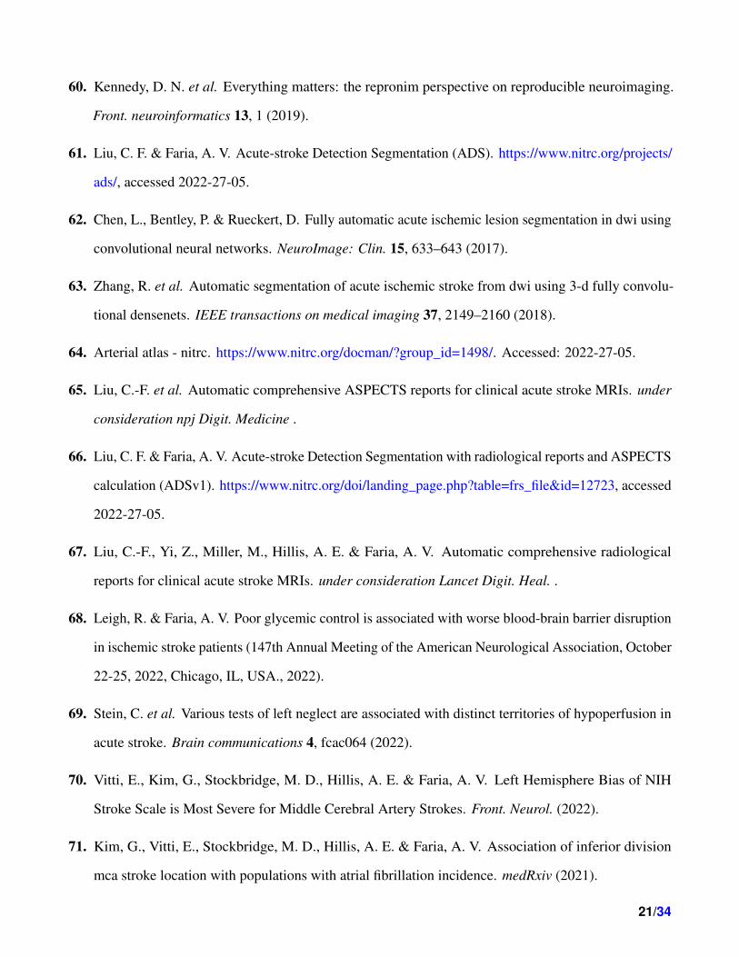
2.5 Probabilistic maps of lesions and “radiological normal” templates

Using the intensity-normalized DWIs in standard space (MNI) of the cases classified as “not-visible”

strokes, we created average and standard deviation maps, here called “radiological normal” templates

(Figure 3). We note that “radiological normal” is an imperfect name, as these cases may still have

abnormalities not directly related to the current stroke episode, such as white matter microvascular chronic

lesions or brain atrophy. Nevertheless, such templates are representative of the radiological aspect of the

brain tissue not directly affected by the acute stroke, of our population. Such templates are potentially

useful for technical development, e.g., for modeling voxel classification by intensity.

We also created frequency maps of the “ischemic” and inrta-parenghymal “hemorrhage” lesions, with

the simple purpose of visualizing the distribution of lesions across the dataset (Figure 4). We performed a

population-based averaging of the lesion masks in MNI space, producing a voxel-wise map where values

can range from 0 at each voxel (no lesion in any subject) to 1 (100% presence of the lesion across subjects).

The frequency maps and the “radiological normal” templates are provided with the dataset. Because the

individual lesion masks are available, users are able to create multiple other types of templates and atlases

that best fit their interest.

3 DISCUSSION

Multimodal public repositories for research data have been organized on the pillars of "FAIR" princi-

ples26: they are designed to be maximally "Findable, Accessible, Interoperable, and Reusable". These

repositories and centralized collections40–44, combined with initiatives to establish semantic and analytical

consensus45, 46, are likely to represent the core structure for future neuroscience research. The sharing of

clinical data, however, is complicated by technical and regulatory issues. While the models of research

data sharing are not adoptable in their exact same form for clinical data, they inspire a similar sharing

structure, respecting the conditions under which the data are usable, without limiting accessibility.

We share the first annotated large dataset of clinical acute stroke MRIs, associated to demographic and

clinical metadata, in alignment with the broad aim of the biomedical community to share FAIR data. The

data organization, in BIDS34 recommended format, is compatible, or can be easily converted to, newly

developed semantic standards, such as the NeuroImaging Data Model (NIDM)45, 47. This provides critical

8/34

capability to generate "computable data objects", that can be readily used by the AI community and are

user-friendly organized to improve access to non-expert data analysts. It also makes easy to integrate

with other ongoing open science efforts27, 40, 48, analytical pipelines49, application program interfaces

(APIs), modules for quality control50, 51 and harmonization52–54, and indexing and management engines55.

These capabilities enable the use of this resource not only for discovery, but also for data synthesis and

augmentation56–58, and to aid reproducibility and replication studies59, 60.

Specifically, the dataset presented here could be used to train, test, or "transfer learning" to algorithms

for lesion segmentation, providing highly important metrics for acute treatment, such as the volume of the

ischemic core and perfusion deficits. For example, we recently used the images with ischemic strokes from

this dataset to developed a public, user-friendly tool to generate "computable data objects"61. We also

developed a public, user-friendly tool for ischemic lesion segmentation and quantification37, overcoming

limitations of previous algorithms not tested in large numbers of real clinical data62, 63. We created the

first public digital atlas of brain arterial territories64, based on the frequency lesion maps of 1,298 of

these cases. This dataset could also be used to develop and test algorithms for mapping low resolution

images of brains with lesions. This mapping allows the examination of the overlap of the lesion with

specific brain structures, like those defined in our arterial territory atlas or others. This enables voxel-based

lesion symptom mapping and the automated calculation of relevant scores, as for example, we did using

this dataset by automatically estimating ASPECTS65, 66. The association of image annotations and lesion

description also enabled us to develop automated image retrieval engines and to generate automated

radiological reports66, 67. Furthermore, this dataset is potentially useful as a general training and testing

resource for translational research. In fact, we initiate several of those efforts by using this dataset and

the tools enabled through it to study laboratory68 and anatomic-functional relations69, to explore bias in

clinical measures70, to study populational trends71, and to test hypothesis developed in external, smaller

datasets.

The main limitation of this dataset is that it originates from a single center. Although we used data from

a certified “Comprehensive Stroke Center”, whose population reflects the profile of the national population

with stroke, and scans with great technical heterogeneity (collected along 10 years, in eleven scanners, and

with dozens of different protocols), a regional bias72 might exist. For instance, our population includes a

9/34

higher percentage of Black and lower percentage of Hispanic/Latinx and Asian patients than many urban

stroke centers. We expect that future sharing and indexing initiatives enable the enrichment of this dataset

with data from multiple other centers. Nevertheless, this dataset will serve as a valuable resource for

training and testing models, particularly those for technical development and for image processing.

4 DATA AVAILABILITY

The dataset is deposited in ICPSR35 (https://doi.org/10.3886/ICPSR38464) and is accessible for

research purposes under data usage agreement. Users are requested to cite the resource and this paper

when using the dataset. Each subject is identified by an 8-digit random code. The data structure, format,

and naming follow the BIDS guidelines, and is as follows (see Figure 1):

1. The main folder “raw-data” contains the image data (“.nii.gz” / “.json” pairs) in the native space of

each subject in two subfolders:

“DWI”, with 4D DWI / B0 and ADC

“anat”, with T1-WI, mprage, T2-WI, FLAIR, PWI, SWI

2. The folder “DWI-mask” contains “.nii.gz” images in native space of

manually-defined lesion masks

brain masks

3D DWI, B0, and “recalculated” ADC

3. The folder “DWI-MNI-IntensityNormalized” contains “.nii.gz” images in standard MNI space,

mapped to JHUSSMNI template39, of

DWI, B0, ADC, lesion mask, brain mask

Intensity-normalized DWI

4. The folder “phenotype” contains

Individual “.tsv” files with metadata of each subject

10/34

The “participants.tsv” with the metadata of the whole dataset

The metadata dictionary, in .txt format (as in this Supplementary Material)

5. The folder "templates" contains the following images in MNI space, according to JHUSSMNI

template39

Average and standard deviation of “radiological normal” DWIs.

Frequency maps of ischemic and hemorrhage lesions.

6. “readme.txt”, describing the general structure of the dataset

“changes.txt”, wich will describe future changes, updates and corrections

5 MATERIALS AND METHODS

5.1 Lesion delineation and agreement between lesion tracers

All the delineations were performed using ROIEditor73. A “seed growing” tool in ROIEditor was often

used to achieve a broad segmentation, followed by manual adjustments. The segmentation was performed

by two individuals highly experienced (more than 10 years) in lesion tracing (JH, XX). Additionally, they

were trained by detailed instructions and illustrative files, in a subset of 220 cases (10% of the dataset cases

with lesions). These cases were then revised by a neuroradiologist (AVF), discussed with the evaluators,

and retrace and revised after 2 weeks. After achieving consensus, the evaluators started working on the

whole dataset. The neuroradiologist revised all the segmentations and identified the suboptimum cases that

were re-traced. The segmentations were revised as many times as necessary, until reaching final decision

by the consensus of the tracers and the neuroradiologist. In the ischemic lesions, the evaluators looked

for hyperintensities in DWI and / or hypointensities (<30% average brain intensity) in ADC. Additional

contrasts were used to rule out chronic lesions or microvascular white matter disease. In the hemorrhage

“lesion type”, extra modalities (SWI, T1WI, T2WI, FLAIR) were used to trace, in addition to DWI.

Extra-parenchymal hemorrhage (intraventricular or subarachnoid) was not traced. The mean time for

tracing was 7 min. The lesion definition was saved as a binary mask (lesion=1, background=0), in the

original image space of each subject.

11/34

We calculated inter-and intra-rater reliability using the Dice similarity coefficient, which indicates

if the same voxels are being selected as part of the lesion mask or not. Values range between 0 and 1

(1 is total agreement). For Dice calculation, we used the set of 220 lesions traced twice. This sample

had the same proportion of ischemic and hemorrhagic lesions as the whole sample. The inter-rater Dice

was 0.68±0.23, while the intra-rater Dice was 0.72±0.14. The agreement was better in ischemic lesions

(0.76±0.14 inter-evaluator and 0.79±0.12 intra-evaluator) compared to hemorrhage. We also calculated

the intraclass correlation coefficient (ICC) for the lesion volumes. The ICC ranges from 0-1; 1 is total

agreement. The inter- and intra-rater ICC were 0.96 and 0.98, respectively. We reinforce that the final

decision for the lesion segmentation in the whole dataset was made after many revisions and by consensus

between the tracers and an expert neuroradiolist.

5.2 Automated skull stripping - BrainMask network

The deep-learning method used for skull stripping, in order to reduce the complexity and computational

time of the process, is described in our previous paper37. Briefly, to generate the gold standards brain

masks, the DWI and B0 images from the "not-visible" cases were resampled into 1× 1× 1 mm3 and

skull striped by a level set algorithm (available with ROIStudio73), with W5 = 1.2 and 4, respectively (see

explanation about choice of parameters in MRIstudio website73). The resulting brain masks (the union

of masking on DWI and B0) were manually corrected by our annotators, serving as ground true for the

"UNet BrainMask Network". To train the network, all images are mapped to MNI and down-sampled to

4×4×4 mm3. The final brain mask inferenced by the network was then post-processed by the closing

and the "binary_fill_holes" functions from Python scipy module, upsampled to 1×1×1 mm3, and dilated

by one voxel with image smoothing. The Dice agreement between the "gold-standard" brain masks and

those obtained with our network was above 99.9%, in an independent test set. The average processing

time was about 19 seconds (against 4.3 min taken by the level-set algorithm73), making it suitable for

large scale, fast processing.

5.3 DWI intensity normalization

The process described here is similar to that descried in our previous publication37, now extended to

the whole dataset, including the cases with hemorrhage lesions.

12/34

Intensity-normalization increases the comparability between subjects and, as normalizing images to a

standardized space, is crucial for diverse image analytical processes. Although the lesion might affect

intensity distribution, we assume that the majority of brain voxels are from healthy tissue and can be a

good reference for intra- and inter-individual comparison. We used bimodal Gaussian function, as in74, in

Equation (1) to fit the intensity histogram of DWI and cluster two groups of voxels: the "brain tissue"

(the highest peak) and "non-brain tissue" (the lowest peak at lowest intensities, composed mostly by

cerebrospinal fluid).

f (x) = a1exp(−(x−b1

c1)2)+a2exp(−(

x−b2

c2)2) (1)

, where ai,bi,ci are the coefficients of the scale, mean, and standard deviation of Gaussian distribution.

ai,bi,ci are calculated by least-square fitting the bimodal Gaussian function to the intensity histogram of

individual DWI. DWI intensities are normalized to make the "brain tissue" intensity with zero mean and

one standard deviation.

Figures 5A show that the DWI intensity distribution of voxels in a brain with ischemic lesions (blue),

one with hemorrhage (green), and in a brain with "not visible" lesion (orange), prior-to (left column)

and post-to (right column) intensity normalization. We note that the preservation of the minor peak at

high intensities in the brain with ischemic lesion indicates the preservation of the lesion contrast after

normalization. Figures 5B-D show the distribution of DWI intensities in groups of images, prior-to (left

column) and post-to (right column) intensity normalization. We note that the distributions are much more

homogeneous, and the individual variations are smaller after intensity normalization. More importantly,

intensity differences between different magnetic fields and scan manufacturers are ameliorated after

intensity normalization.

We also note that this normalization approach helped to reduce the complexity and time to train

Deep Learning Networks for ischemic lesion segmentation. We experimented training UNet with DWIs

normalized by our proposed method (‘ProposedNorm’) and three others: 1) standard z-score normalization

on whole images (‘StandardNorm’), 2) standard z-score normalization on brain-masked region only

(‘BrainMaskStandardNorm’), and 3) Max-Min normalization (‘MaxMinNorm’). We kept all other

procedures for training the network, inferencing predicts, and the post-processing the same, as described

13/34

in37. We used the intensity normalized DWI and ADC as inputs, and 5-fold cross-validation. Table 2

shows that the Dice scores between automated and manually traced images were higher when using images

intensity-normalized with the proposed method.

Finally, in addition to the ADC from the scanners, we offer ADCs “recalculated” as:

IADC(x,y,z) =lnI(x,y,z)− lnI0(x,y,z)

b(2)

, where I(x,y,z), I0(x,y,z) are the intensity of DWI and B0 voxels, respectively, at (x,y,z)-coordinate, with

b-value = 1000.

5.4 Quality control for images in standardized space, MNI

Clinical images offer extra challenges for brain mapping to standardized space, because of their high

slice thickness and fair amount of tilt out-of-plane, therefore requiring further stringent quality control.

The quality control of the normalized images was performed in two steps: 1) qualitative: a neuroradiologist

looked at the MNI-normalized images with the MNI template brain mask overlaid, in order to rule-out

obvious misalignments, and 2) quantitative: performed as described below.

a) Three regions of 5 voxels bandwidth were defined in the template: the outside strip of the brain

mask (OSBM), the inside strip of the brain mask (ISBM), and the outside strip of the lateral ventricles

(OSLV), as shown in Figure 6, top.

b) The ratio of the mis-deformed voxels in OSBM, ISBM and OSLV for each subject, defined as

γOSBM, γISBM, and γOSLV, was calculated as follows:

γOSBM =the number of the deformed B0 voxels whose intensity is larger than 0 in OSBM

the number of voxels in OSBM(3)

γISBM =the number of the deformed B0 voxels whose intensity is 0 in ISBM

the number of voxels in ISBM(4)

γOSLV =the number of the deformed B0 voxels whose intensity is larger than λ in OSLV

the number of voxels in OSLV(5)

λ = µdeformed B0 in LV−0.5×σdeformed B0 in LV (6)

14/34

γOSBM indicates the ratio of the deformed B0 voxels aligned outside the template brain mask and

γISBM indicates the ratio of the background voxels aligned inside the template brain mask. High γOSBM

or γISBM indicte possible issues with the global brain mapping. γOSLV indicates the ratio of voxels from

a subject’s deformed ventricles that exist outside the template lateral ventricle boundaries. High γOSLV is

common in this population since aged subjects’ lateral ventricles are usually larger than the template’s

lateral ventricles and indicate the need for local, and possibly non-linear deformation for brain mapping.

The average γOSBM was 0.2042 ± 0.0628 (medium=0.1929, range [0.0723, 0.5070]). The average

γISBM was 0.2683 ± 0.0426 (medium=0.2666, range [0.1560, 0.4273]). This means that a small minority

of voxels were outer or inner the template brain contour, when considering a stringent bandwidth of

5 voxels. Importantly, the small ratio of error was stable over stroke types, magnetic field, or scan

manufacturer (Figure 6).

Acknowledgements

We thank Sandhya Ramachandran, Xuejie Wang, Isabella Lorence, Akuna Mezu, Mah Noor, Esthefani

Garcia, and Jonathan B. A. Assuncao for technical assistance. This research was supported by the:

National Institute of Deaf and Communication Disorders, NIDCD, through R01 DC05375, R01

DC015466, P50 DC014664 (AEH. AVF)

National Institute of Biomedical Imaging and Bioengineering, NIBIB, through P41 EB031771 (SM,

AVF).

Author contribution

AVF and CL conceived and designed the study, analyzed, and interpreted the data, drafted the work.

JH, XX, XL analyzed the data. RL, BJ, VU, AEH acquired the data and revised the draft. SM revised the

draft.

Competing interests

We report the following competing interest: Susumu Mori owns “AnatomyWorks”. This arrangement

is being managed by the Johns Hopkins University in accordance with its conflict-of-interest policies. The

15/34

reaming authors have no competing interest.

References

1. Virani, S. S. et al. Heart disease and stroke statistics—2020 update: a report from the american heart

association. Circulation 141, e139–e596 (2020).

2. Gajardo-Vidal, A. et al. How distributed processing produces false negatives in voxel-based lesion-

deficit analyses. Neuropsychologia 115, 124–133 (2018).

3. Lorca-Puls, D. L. et al. The impact of sample size on the reproducibility of voxel-based lesion-deficit

mappings. Neuropsychologia 115, 101–111 (2018).

4. Mah, Y.-H., Husain, M., Rees, G. & Nachev, P. Human brain lesion-deficit inference remapped. Brain

137, 2522–2531 (2014).

5. Shahid, H. et al. Important considerations in lesion-symptom mapping: Illustrations from studies of

word comprehension. Hum. brain mapping 38, 2990–3000 (2017).

6. Wilson, S. M. Lesion-symptom mapping in the study of spoken language understanding. Lang. Cogn.

Neurosci. 32, 891–899 (2017).

7. Esteva, A. et al. Deep learning-enabled medical computer vision. npj digit. Med 4, 1–9 (2021).

8. Geirhos, R. et al. Shortcut learning in deep neural networks. Nat. Mach. Intell. 2, 665–673 (2020).

9. Willemink, M. J. et al. Preparing medical imaging data for machine learning. Radiology 295, 4–15

(2020).

10. Armato III, S. G. et al. The lung image database consortium (lidc) and image database resource

initiative (idri): a completed reference database of lung nodules on ct scans. Med. physics 38, 915–931

(2011).

11. Bejnordi, B. E. et al. Diagnostic assessment of deep learning algorithms for detection of lymph node

metastases in women with breast cancer. Jama 318, 2199–2210 (2017).

12. Halling-Brown, M. D. et al. Optimam mammography image database: a large-scale resource of

mammography images and clinical data. Radiol. Artif. Intell. 3, e200103 (2020).

16/34

13. Irvin, J. et al. Chexpert: A large chest radiograph dataset with uncertainty labels and expert comparison.

In Proceedings of the AAAI conference on artificial intelligence, vol. 33, 590–597 (2019).

14. Tschandl, P., Rosendahl, C. & Kittler, H. The ham10000 dataset, a large collection of multi-source

dermatoscopic images of common pigmented skin lesions. Sci. data 5, 1–9 (2018).

15. Wang, X. et al. Chestx-ray8: Hospital-scale chest x-ray database and benchmarks on weakly-

supervised classification and localization of common thorax diseases. In Proceedings of the IEEE

conference on computer vision and pattern recognition, 2097–2106 (2017).

16. Simpson, A. L. et al. A large annotated medical image dataset for the development and evaluation of

segmentation algorithms. arXiv preprint arXiv:1902.09063 (2019).

17. Broderick, J. et al. The greater cincinnati/northern kentucky stroke study: preliminary first-ever and

total incidence rates of stroke among blacks. Stroke 29, 415–421 (1998).

18. D’Agostino, R. B., Wolf, P. A., Belanger, A. J. & Kannel, W. B. Stroke risk profile: adjustment for

antihypertensive medication. the framingham study. Stroke 25, 40–43 (1994).

19. Wintermark, M. et al. Acute stroke imaging research roadmap. Stroke 39, 1621–1628 (2008).

20. Albers, G. W. et al. A multicenter randomized controlled trial of endovascular therapy following

imaging evaluation for ischemic stroke (defuse 3) (2017).

21. Giese, A.-K. et al. Design and rationale for examining neuroimaging genetics in ischemic stroke: The

mri-genie study. Neurol. Genet. 3 (2017).

22. Nagakane, Y. et al. Epithet: positive result after reanalysis using baseline diffusion-weighted

imaging/perfusion-weighted imaging co-registration. Stroke 42, 59–64 (2011).

23. Sandercock, P., Wardlaw, J., Lindley, R., Whiteley, W. & Cohen, G. Ist-3 stroke trial data available.

The Lancet 387, 1904 (2016).

24. Saver, J., Goyal, M., Bonafe, A. et al. Stent-retriever thrombectomy after intravenous t-pa vs. t-pa

alone in stroke [published online april 17, 2015]. N Engl J Med. doi 10.

17/34

25. Thomalla, G. et al. Dwi-flair mismatch for the identification of patients with acute ischaemic stroke

within 4· 5 h of symptom onset (pre-flair): a multicentre observational study. The Lancet Neurol. 10,

978–986 (2011).

26. Wilkinson, M. D. et al. The fair guiding principles for scientific data management and stewardship.

Sci. data 3, 1–9 (2016).

27. Sansone, S.-A. et al. Fairsharing as a community approach to standards, repositories and policies.

Nat. biotechnology 37, 358–367 (2019).

28. Maier, O. et al. Isles 2015-a public evaluation benchmark for ischemic stroke lesion segmentation

from multispectral mri. Med. image analysis 35, 250–269 (2017).

29. Liew, S.-L. et al. A large, open source dataset of stroke anatomical brain images and manual lesion

segmentations. Sci. data 5, 1–11 (2018).

30. Liew, S.-L. et al. The enigma stroke recovery working group: Big data neuroimaging to study

brain–behavior relationships after stroke. Hum. brain mapping (2020).

31. Bing, Y., Garcia-Gonzalez, D., Voets, N. & Jérusalem, A. Medical imaging based in silico head model

for ischaemic stroke simulation. J. mechanical behavior biomedical materials 101, 103442 (2020).

32. Sharique, M., Pundarikaksha, B. U., Sridar, P., Krishnan, R. R. & Krishnakumar, R. Parallel capsule

net for ischemic stroke segmentation. bioRxiv 661132 (2019).

33. Wang, Y., Juliano, J. M., Liew, S.-L., McKinney, A. M. & Payabvash, S. Stroke atlas of the brain:

Voxel-wise density-based clustering of infarct lesions topographic distribution. NeuroImage: Clin. 24,

101981 (2019).

34. Gorgolewski, K. J. et al. The brain imaging data structure, a format for organizing and describing

outputs of neuroimaging experiments. Sci. data 3, 1–9 (2016).

35. Faria, A. V. Annotated Clinical MRIs and Linked Metadata of Patients with Acute Stroke, Baltimore,

Maryland, 2009-2019. https://doi.org/10.3886/ICPSR38464.v1, accessed 2022-27-05.

18/34

36. Wheeler, H. M. et al. The growth rate of early dwi lesions is highly variable and associated with

penumbral salvage and clinical outcomes following endovascular reperfusion. Int. J. Stroke 10,

723–729 (2015).

37. Liu, C.-F. et al. Deep learning-based detection and segmentation of diffusion abnormalities in acute

ischemic stroke. Commun. Medicine 1, 1–18 (2021).

38. Woods, R. P., Grafton, S. T., Holmes, C. J., Cherry, S. R. & Mazziotta, J. C. Automated image

registration: I. general methods and intrasubject, intramodality validation. J. computer assisted

tomography 22, 139–152 (1998).

39. Mori, S. et al. Stereotaxic white matter atlas based on diffusion tensor imaging in an icbm template.

Neuroimage 40, 570–582 (2008).

40. Markiewicz, C. J. et al. Openneuro: An open resource for sharing of neuroimaging data. bioRxiv

(2021).

41. Landis, D. et al. Coins data exchange: An open platform for compiling, curating, and disseminating

neuroimaging data. NeuroImage 124, 1084–1088 (2016).

42. Neu, S. C., Crawford, K. L. & Toga, A. W. Sharing data in the global alzheimer’s association

interactive network. Neuroimage 124, 1168–1174 (2016).

43. Crawford, K. L., Neu, S. C. & Toga, A. W. The image and data archive at the laboratory of neuro

imaging. Neuroimage 124, 1080–1083 (2016).

44. Kennedy, D. N., Haselgrove, C., Riehl, J., Preuss, N. & Buccigrossi, R. The nitrc image repository.

NeuroImage 124, 1069–1073 (2016).

45. Keator, D. B. et al. Towards structured sharing of raw and derived neuroimaging data across existing

resources. Neuroimage 82, 647–661 (2013).

46. Larson, S. D. & Martone, M. Neurolex. org: an online framework for neuroscience knowledge. Front.

neuroinformatics 7, 18 (2013).

47. NIDM. https://github.com/incf-nidash/PyNIDM, accessed 2021-10-11.

19/34

48. Group, D. M. W. Datacite metadata schema documentation for the publication and citation of research

data and other research outputs. https://doi.org/10.14454/3w3z-sa82 Version 4.4. DataCite e.V

(2021).

49. brainlife. https://brainlife.io/, accessed 2021-10-12.

50. Klapwijk, E. T., Van De Kamp, F., Van Der Meulen, M., Peters, S. & Wierenga, L. M. Qoala-t:

A supervised-learning tool for quality control of freesurfer segmented mri data. Neuroimage 189,

116–129 (2019).

51. Kim, H. et al. The loni qc system: a semi-automated, web-based and freely-available environment for

the comprehensive quality control of neuroimaging data. Front. neuroinformatics 13, 60 (2019).

52. Ning, L. et al. Cross-scanner and cross-protocol multi-shell diffusion mri data harmonization:

Algorithms and results. NeuroImage 221, 117128 (2020).

53. Garcia-Dias, R. et al. Neuroharmony: A new tool for harmonizing volumetric mri data from unseen

scanners. NeuroImage 220 (2020).

54. Da-Ano, R. et al. Performance comparison of modified combat for harmonization of radiomic features

for multicenter studies. Sci. Reports 10, 1–12 (2020).

55. Halchenko, Y. O. et al. Datalad: distributed system for joint management of code, data, and their

relationship. J. Open Source Softw. 6, 3262 (2021).

56. Dar, S. U. et al. Image synthesis in multi-contrast mri with conditional generative adversarial networks.

IEEE transactions on medical imaging 38, 2375–2388 (2019).

57. Xia, T., Chartsias, A. & Tsaftaris, S. A. Pseudo-healthy synthesis with pathology disentanglement

and adversarial learning. Med. Image Analysis 64, 101719 (2020).

58. Bowles, C. et al. Brain lesion segmentation through image synthesis and outlier detection. NeuroImage:

Clin. 16, 643–658 (2017).

59. Botvinik-Nezer, R. et al. Variability in the analysis of a single neuroimaging dataset by many teams.

Nature 582, 84–88 (2020).

20/34

60. Kennedy, D. N. et al. Everything matters: the repronim perspective on reproducible neuroimaging.

Front. neuroinformatics 13, 1 (2019).

61. Liu, C. F. & Faria, A. V. Acute-stroke Detection Segmentation (ADS). https://www.nitrc.org/projects/

ads/, accessed 2022-27-05.

62. Chen, L., Bentley, P. & Rueckert, D. Fully automatic acute ischemic lesion segmentation in dwi using

convolutional neural networks. NeuroImage: Clin. 15, 633–643 (2017).

63. Zhang, R. et al. Automatic segmentation of acute ischemic stroke from dwi using 3-d fully convolu-

tional densenets. IEEE transactions on medical imaging 37, 2149–2160 (2018).

64. Arterial atlas - nitrc. https://www.nitrc.org/docman/?group_id=1498/. Accessed: 2022-27-05.

65. Liu, C.-F. et al. Automatic comprehensive ASPECTS reports for clinical acute stroke MRIs. under

consideration npj Digit. Medicine .

66. Liu, C. F. & Faria, A. V. Acute-stroke Detection Segmentation with radiological reports and ASPECTS

calculation (ADSv1). https://www.nitrc.org/doi/landing_page.php?table=frs_file&id=12723, accessed

2022-27-05.

67. Liu, C.-F., Yi, Z., Miller, M., Hillis, A. E. & Faria, A. V. Automatic comprehensive radiological

reports for clinical acute stroke MRIs. under consideration Lancet Digit. Heal. .

68. Leigh, R. & Faria, A. V. Poor glycemic control is associated with worse blood-brain barrier disruption

in ischemic stroke patients (147th Annual Meeting of the American Neurological Association, October

22-25, 2022, Chicago, IL, USA., 2022).

69. Stein, C. et al. Various tests of left neglect are associated with distinct territories of hypoperfusion in

acute stroke. Brain communications 4, fcac064 (2022).

70. Vitti, E., Kim, G., Stockbridge, M. D., Hillis, A. E. & Faria, A. V. Left Hemisphere Bias of NIH

Stroke Scale is Most Severe for Middle Cerebral Artery Strokes. Front. Neurol. (2022).

71. Kim, G., Vitti, E., Stockbridge, M. D., Hillis, A. E. & Faria, A. V. Association of inferior division

mca stroke location with populations with atrial fibrillation incidence. medRxiv (2021).

21/34

72. Howard, V. J. et al. The reasons for geographic and racial differences in stroke study: objectives and

design. Neuroepidemiology 25, 135–143 (2005).

73. MRI Studio. https://www.mristudio.org, accessed 2021-05-14.

74. Shinohara, R. T. et al. Statistical normalization techniques for magnetic resonance imaging. NeuroIm-

age: Clin. 6, 9–19 (2014).

Figures and Tables

Figure 1. Overall description of the archive, which follows BIDS recommendations for structure and

naming. All images are anonymized, in “.nii.gz/.json” format. The itemized description of the metadata (*

in “.tsv” format) is in the “Dictionary”, included in the dataset and here, as Supplementary Material. The

summary of the demographic and clinical information for the cohort is in Table 1

.

22/34

Figure 2. Dataset lesion and image profiles. Distribution of lesions attributed to ischemia or hemorrhage

according to (a) volumes, (b) arterial territories, (c) brain structures. (d) Presence of MRI modalities other

than DWI. Note that although the categorization in arterial territories is not necessarily meaningful for

hemorrhage, we offer it for the sake of an uniform description23/34

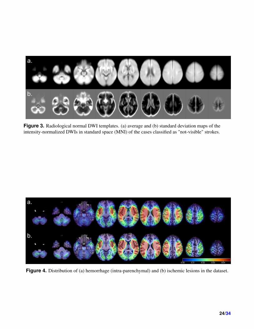
Figure 3. Radiological normal DWI templates. (a) average and (b) standard deviation maps of the

intensity-normalized DWIs in standard space (MNI) of the cases classified as "not-visible" strokes.

Figure 4. Distribution of (a) hemorrhage (intra-parenchymal) and (b) ischemic lesions in the dataset.

24/34

Figure 5. Probability distribution (y axis) of DWIs’ voxel intensity (x axis) prior-to (left column) and

post-to (right column) intensity normalization. Panel (a) shows the distributions of DWI intensities of a

selected cases with ischemic lesion (blue), hemorrhage (green), and "not visible" lesion (orange). Panels

(b), (c), and (d) show the distributions of DWI intensities in groups according to presence of visible

ischemic abnormality or hemorrhage (b), magnetic fields (c), and scanner manufacturers (d). The solid

line is the average group distribution, the shadowed area is within 1 standard deviation from average.25/34

Figure 6. Quality control of the image mapping to standard coordinates (MNI). The top figure illustrates

the three regions of 5 voxels bandwidth defined in the template: the outside strip of the brain mask

(OSBM), the inside strip of the brain mask (ISBM), and the outside strip of the lateral ventricles (OSLV).

The bottom boxplots illustrate the average of OSBM and ISBM (γOSBM and γISBM), which are

indicative of the global quality of the brain mapping, across lesion type, magnetic field and scan

manufacturer

26/34

DatasetTotal Ischemic Hemorrhagic Not Visible

(n = 2888) (n = 1878, 70%) (n = 540, 12%) (n = 470, 18%)

Dem

og

rap

hic

s

Age in years 62.00[53,73]; 0 62.00[53,72]; 0 64.00[54,75]; 0 61.00[52,71]; 0

Sex

Female 1361(47.13%) 866(46.11%) 259(47.96%) 236(50.21%)

Male 1527(52.87%) 1012(53.89%) 281(52.04%) 234(49.79%)

Race

African American 1257 (43.52%) 824 (43.88%) 210 (38.89%) 223 (47.45%)

Caucasian 918 (31.79%) 533 (28.38%) 206 (38.15%) 179 (38.09%)

Asian 76 (2.63%) 44 (2.34%) 25 (4.63%) 7 (1.49%)

Not Recorded 637 (22.06%) 477 (25.40%) 99 (18.33%) 61 (12.98%)

Cli

nic

sa

nd

lab

ora

tori

al

test

sa

th

osp

ita

la

dm

issi

on

NIHSS 3.00[1.00,8.00]; 1403 4.00[1.00,8.00]; 804 8.00[3.00,13.75]; 354 1.00[0.00,3.00]; 245

Systolic 154.00[136.00,178.00]; 508 155.00[137.00,180.00]; 401 154.00[133.00,172.00]; 58 150.00[133.00,173.00]; 49

Diastolic 83.00[73.00,95.00]; 508 84.00[74.00,96.00]; 401 81.00[72.00,96.75]; 58 81.00[72.00,92.00]; 49

Cholesterol 167.00[137.00,201.00]; 707 168.00[137.00,203.00]; 452 162.00[134.75,194.25]; 168 168.00[140.50,202.00]; 87

Triglycerides 100.00[72.00,144.50]; 717 102.00[73.00,146.00]; 460 91.00[67.75,128.00]; 168 101.00[72.00,156.00]; 89

HDL 46.00[36.00,57.00]; 710 45.00[36.00,57.00]; 455 47.00[37.00,59.00]; 168 47.00[38.00,59.00]; 87

LDL 95.00[70.00,124.00]; 712 96.00[71.00,125.00]; 455 92.00[67.00,115.00]; 171 95.00[69.00,124.00]; 86

Hemoglobin A1C 5.80[5.40,6.60]; 805 5.90[5.40,6.70]; 514 5.70[5.40,6.50]; 178 5.80[5.40,6.40]; 113

Glucose 0.90[0.80,1.20]; 509 113.00[98.00,146.00]; 451 125.00[104.00,159.00]; 79 107.00[94.00,131.00]; 59

Creatinine 0.90[0.80,1.20]; 509 1.00[0.80,1.20]; 400 0.90[0.70,1.20]; 59 0.90[0.80,1.10]; 50

Prothrombin 1.00[1.00,1.10]; 675 1.00[1.00,1.10]; 518 1.10[1.00,1.10]; 72 1.00[1.00,1.10]; 85

BMI 27.68[24.03,32.45]; 808 27.82[24.07,32.46]; 557 27.37[23.95,31.77]; 134 27.45[24.04,33.31]; 117

Days at hospital 4.00[2.00,8.00]; 829 4.00[2.00,7.00]; 567 7.00[4.00,14.00]; 123 2.00[1.00,4.00]; 139

Prior medical conditions

Hypertension 1756 (60.80%) 1124 (59.85%) 346 (64.07%) 286 (60.85%)

Dyslipidemia 915 (31.68%) 592 (31.52%) 147 (27.22%) 176 (37.45%)

Diabetes mellitus 741 (25.66%) 481 (25.61%) 139 (25.74%) 121 (25.74%)

Previous stroke 634 (21.95%) 409 (21.78%) 122 (22.59%) 103 (21.91%)

Smoker 620 (21.47%) 434 (23.11%) 88 (16.30%) 98 (20.85%)

Atrial Fib/Flutter 272 (9.42%) 167 (8.89%) 68 (12.59%) 37 (7.87%)

coronary dis./prior heart infarct 383 (13.26%) 232 (12.35%) 78 (14.44%) 73 (15.53%)

Obesity/Overweight 225 (7.79%) 149 (7.93%) 35 (6.48%) 41 (8.72%)

Chronic renal insufficiency 114 (3.95%) 82 (4.37%) 23 (4.26%) 9 (1.91%)

Family history of stroke 111 (3.84%) 75 (3.99%) 22 (4.07%) 14 (2.98%)

Heat failure 109 (3.77%) 75 (3.99%) 21 (3.89%) 13 (2.77%)

Migraine 83 (2.87%) 52 (2.77%) 16 (2.96%) 15 (3.19%)

Sleep apnea 57 (1.97%) 40 (2.13%) 9 (1.67%) 8 (1.70%)

Peripheral vascular disease 40 (1.39%) 25 (1.33%) 6 (1.11%) 9 (1.91%)

Carotid Stenosis 26 (0.90%) 17 (0.91%) 6 (1.11%) 3 (0.64%)

Prosthetic heart valve 14 (0.48%) 6 (0.32%) 4 (0.74%) 4 (0.85%)

Sickle cell 10 (0.35%) 6 (0.32%) 3 (0.56%) 1 (0.21%)

Current pregancy 3 (0.10%) 2 (0.11%) 0 (0.00%) 1 (0.21%)

Hormone replacement 3 (0.10%) 2 (0.11%) 0 (0.00%) 1 (0.21%)

Vein thromb./pulmonary emb. 2 (0.07%) 1 (0.05%) 1 (0.19%) 0 (0.00%)

Not Recorded 665 (23.03%) 482 (25.67%) 95 (17.59%) 88 (18.72%)

Prior Medication

Anticholesterol 966 (33.45%) 624 (33.23%) 174 (32.22%) 168 (35.74%)

Anticoagulants 197 (6.82%) 100 (5.32%) 59 (10.93%) 38 (8.09%)

Antiglucose 546 (18.91%) 361 (19.22%) 87 (16.11%) 98 (20.85%)

Antihypertensive 1540 (53.32%) 974 (51.86%) 294 (54.44%) 272 (57.87%)

Antiplatelet 1000 (34.63%) 630 (33.55%) 187 (34.63%) 183 (38.94%)

Not Recorded 1088 (37.67%) 748 (39.83%) 195 (36.11%) 145 (30.85%)

MR

Ia

nd

lesi

on

cha

ract

eris

tics

Hours from symptomns to MRI

<2 150 (5.19%) 104 (5.54%) 21(3.89%) 25(5.32%)

2-6 339 (11.74%) 241 (12.83%) 42(7.78%) 56(11.91%)

6-12 348 (12.05%) 232 (12.35%) 60(11.11%) 56(11.91%)

12-24 827 (28.64%) 500 (26.62%) 158(29.26%) 169(35.96%)

>24 287 (9.94%) 122 (6.50%) 124(22.96%) 41(8.72%)

missing 937 (32.44%) 679 (36.16%) 135(25%) 123(26.17%)

MRI Magnetic Field

1.5T 1766 (61.15%) 1217(64.80%) 252(46.67%) 297(63.19%)

3.0T 1122 (38.85%) 661 (35.20%) 288 (53.33%) 173 (36.81%)

Scan manufacturer

Siemens 2614 (90.51%) 1667 (88.76%) 517 (95.74%) 430 (91.49%)

Philips 22 (0.76%) 15 (0.80%) 2 (0.37%) 5 (1.06%)

GE 210 (7.27%) 166 (8.84%) 17 (3.15%) 27 (5.74%)

Not Recorded 42 (1.45%) 30 (1.60%) 4 (0.74%) 8 (1.70%)

Thrombolisis pre-scan

Yes 1251 (43.32%) 931 (49.57%) 98 (18.15%) 222(47.23%)

No 1637 (56.68%) 947 (50.43%) 442 (81.85%) 248 (52.77%)

DWIvoxsize 5.74[3.20,7.20] 5.72[3.20,7.60] 5.74[3.20,7.20] 5.74[3.53,7.60]

Lesion volume in ml 7.86[1.46,32.34] 4.27[0.98,22.12] 30.27[12.51,68.55] N.A.

Hemisphere

Left 1082 (37.47%) 834 (44.41%) 248 (45.93%)

N.A.Right 976 (33.80%) 766 (40.79%) 210 (38.89%)

Bilateral 360 (12.47%) 278 (14.80%) 82 (15.19%)

Diagnosis

Embolic Stroke 22 (0.76%) 19 (1.01%) 2 (0.37%) 1 (0.21%)

Intra Cerebral Hemorrhage 381 (13.19%) 18 (0.96%) 346 (64.07%) 17 (3.62%)

Ischecmi Stroke 2164 (74.93%) 1794 (95.53%) 166 (30.74%) 204 (43.4%)

Subarachmoid Hemorrhage 81 (2.8%) 25 (1.33%) 22 (4.07%) 34 (7.23%)

Transitory Ischemic Acident 240 (8.31%) 22 (1.17%) 4 (0.74%) 214 (45.53%)

Table 1. Demographic and clinical profile of the population; MRI and lesion characteristics. Continuous

data is presented as median[interquartile range]; missing value. Categorical variables are presented by the

numbers and % they represent in each group.27/34

ProposedNorm StandardNorm BrainMaskStandardNorm MaxMinNorm

Validation 0.75(0.17); 0.80 0.64(0.22); 0.70 0.48(0.29); 0.51 0.54(0.24); 0.61

Testing 0.74(0.20); 0.80 0.64(0.21); 0.70 0.53(0.31); 0.62 0.53(0.23); 0.60

Table 2. Accuracy of the same UNET Deep Learning model on segmenting ischemic core, using DWIs

normalized by different methods. The normalization methods tested were: ’ProposedNorm’: described in

this manuscript; ‘StandardNorm’: standard z-score normalization on whole images;

‘BrainMaskStandardNorm’: standard z-score normalization on brain-masked region only;

‘MaxMinNorm’: Max-Min normalization. Except for the intensity normalization, all procedures for

training the network, inferencing predicts, and the post-processing are the same (as in37). The numbers

represent the average (standard deviation); media of Dice scores between the automatically and manually

traced images, in the 5-fold cross-validation (total training sample=1849) and testing samples (499).

28/34

Supplementary Material: Metadata Dictionary

Age

Description age of the participant

Units years (<30 for 30 years-old and younger, >90 for 90 years-old and older)

Sex

Description sex of the participant reported by the participant

Levels M: male

F: female

Race

Description race of the participant reported by the participant

Levels BAA: Black or African American

W: white

A: Asian

O: other

NA: not available

Diagnosis

Description clinical diagnosis at admission

Levels IS: Ischemic Stroke

ES: Embolic Stroke

ICH: Intracranial Hemorrhage

TIA: Transitory Ischemic Accident

SAH: Subarachnoid Hemorrhage

Medical-history

Description previous medical conditions reported by the participant or available on medical charts

at admission

Levels Hypertension: history of systolic blood pressure >=130mmHg or diastolic

>=80mmHg or use of anti-hypertensive medication

29/34

Dyslipidemia: medical history of dyslipidemia or use of anti-cholesterol medication

Diabetes Mellitus: history of diabetes or use of anti-glucose medication

Smoker: smoke status as reported by the participant

Previous Stroke: history of stroke as reported by the participant or by medical chart

CAD/prior MI: Coronary arterial disease or prior myocardial infarct

Previous TIA: history of transitory ischemic accident

Family History of Stroke: first relative history of stroke as reported by the participant

Atrial Fib/Flutter: history of Atrial Fibrillation or atrial Flutter

HF: Heart Failure as reported by the participant or by medical chart

Prosthetic Heart Valve: history of Prosthetic Heart Valve

Renal Insufficiency – chronic: renal insufficiency as reported by participant or by

chart

Migraine: history of migraine as reported by participant

Obesity / Overweight: obesity or overweight reveled by history of BMI at admission

PVD: history of peripheral vascular disease

Carotid Stenosis: history of carotid stenosis

Sleep Apnea: history of sleep apnea as reported by the participant or by medical

chart

Prior-medication

Description previous use of listed medications as reported by the participant or available on

medical charts at admission

Levels Antihypertensive: Antihypertensive drug

Antiglucose: Antiglucose drug

Anticholesterol: Anticholesterol drug

Antiplatet: Antiplatet drug

Anticoagulant: Anticoagulant drug

Ambulation-prior

Description ability to walk prior to the admission as reported by the participant

30/34

Levels 1: Able to ambulate independently (no help from another person, w/ or w/o device)

2: With assistance (from person)

3: Unable to ambulate

NIHSS

Description The National Institutes of Health Stroke Scale at admission exam

TermURL https://www.stroke.nih.gov/documents/NIH_Stroke_Scale_508C.pdf

Ambulation-arrival

Description ability to walk at hospital arrival

Levels 1. Able to ambulate independently (no help from another person, w/ or w/o device)

2. With assistance (from person)

3. Unable to ambulate

IVtPA

Description Thrombolysis with intravenous tissue-type plasminogen activator performed before

the MRI scan in the dataset

Levels 1. Yes

2. No

Systolic

Description systolic blood pressure at hospital arrival

Units mm Hg

Diastolic

Description systolic blood pressure at hospital arrival

Units mm Hg

Cholesterol

Description total blood cholesterol level at first laboratorial exam after hospital arrival

Units mg/dL

Triglycerides

Description triglycerides level at first laboratorial exam after hospital arrival

31/34

Units mg/dL

HDL

Description High-density lipoprotein cholesterol level at first laboratorial exam

Units mg/dL

LDL

Description Low-density lipoprotein cholesterol level at first laboratorial exam

Units mg/dL

hba1c

Description Hemoglobin A1c at first laboratorial exam after hospital arrival

Units %

Glucose

Description Blood fasting glucose level at first laboratorial exam after hospital arrival

Units mg/dL

Creatinine

Description Serum creatinine level at first laboratorial exam after hospital arrival

Units mg/dL

Prothrombin

Description Prothrombin time at first test after hospital arrival

Units International Normalized Ratio, INR

BMI

Description Body mass index of the participant

Units kg/m2

Ambulation-discharge

Description ability to walk at hospital discharge

Levels 1. Able to ambulate independently (no help from another person) w/ or w/o device)

2. With assistance (from person)

3. Unable to ambulate

Hospitalizatoin days

32/34

Description Time of hospital stay

Units days

Symptoms-MRI

Description Hours between symptoms as reported by the participant and MRI scan

Levels <2

2-6

6-12

13-24

>24

Lesion-type

Description Stroke lesion appearance at MRI, according radiological diagnosis

Levels ischemic: DWI hyperintensity + ADC hypo/isointensity, per radiological interpreta-

tion

hemorrhagic: any signal of bleeding, intra- or extra-parenchymal, per radiological

interpretation. It includes primarily hemorrhagic strokes and hemorrhagic transfor-

mation of ischemic strokes.

not visible: ischemic area is not visible, per radiological interpretation. It does not

include ischemic areas detected retrospectively (after a follow up scan or automated

detection).

Side

Description Stroke hemisphere according to MRI

Levels Left

Right

Bilateral

MR-field

Description Magnetic Field of the MR scan, in tesla

Levels 3

1.5

33/34

MR-manufacturer

Description MR scan manufacturer

Levels 1. Siemens

2. Phillips

3. GE

4. Not Recorded

Other-MRI-modalities

Description Available MRI modalities, in addition to the DWI

Levels ADC: apparent diffusion coefficient

FLAIR: Fluid-attenuated inversion recovery, defaced if high resolution out-plane

mprage: high resolution T1weighted image, defaced

PWI: perfusion weighted image

SWI: susceptibility weighted image

T1w: T1-weighted images, defaced if high resolution out-plane

T1wC: T1-weighted images, post-contrast iv injection, defaced if high resolution

out-plane

T2w: T2-weighted images, defaced if high resolution out-plane

DWI-voxel-size

Description DWI voxel width x voxel height x slice thickness (plus gap)

Units mm3

Stroke-volume

Description Volume of the stroke (number of voxels x voxel size) as described by the manual

delineation of the MRI lesion

Units mm3

34/34