A large H survey at z = 2.23, 1.47, 0.84 and 0.40: the 11 Gyr evolution of star-forming galaxies...

Mon. Not. R. Astron. Soc. 000, 1–18 (2012) Printed 17 February 2012 (MN LATEX style file v2.2)

A large, multi-epoch Hα survey at z = 2.23,1.47,0.84&0.40: the11 Gyr evolution of star-forming galaxies from HiZELS?

David Sobral1†, Ian Smail2, Philip N. Best3, James E. Geach4, Yuichi Matsuda5,John P. Stott2, Michele Cirasuolo4,6 & Jaron Kurk71 Leiden Observatory, Leiden University, P.O. Box 9513, NL-2300 RA Leiden, The Netherlands2 Institute for Computational Cosmology, Durham University, South Road, Durham, DH1 3LE, UK3 SUPA, Institute for Astronomy, Royal Observatory of Edinburgh, Blackford Hill, Edinburgh, EH9 3HJ, UK4 Department of Physics, McGill University, Ernest Rutherford Building, 3600 Rue University, Montreal, Quebec, Canada, H3A 2T85 Cahill Center for Astronomy & Astrophysics, California Institute of Technology, MS 249-17, Pasadena, CA 91125, USA6 UK Astronomy Technology Centre, Royal Observatory, Blackford Hill, Edinburgh EH9 3HJ7 Max-Planck-Institut fur Astrophysik, Karl-Schwarzschild Strasse 1, D-85741 Garching, Germany

17 February 2012

ABSTRACTThis paper presents new deep and wide narrow-band surveys undertaken with UKIRT, Subaruand the VLT; a unique combined effort to select large, robust samples of Hα star-forminggalaxies at z = 0.40, 0.84, 1.47 and 2.23 (corresponding to look-back times of 4.2, 7.0,9.2 and 10.6 Gyrs) in a uniform manner over ∼ 2 deg2 in the COSMOS and UDS fields.The deep multi-epoch Hα surveys reach a matched 3σ flux limit of ≈ 3 M yr−1 out toz = 2.2 for the first time, while the wide area and the coverage over two independent fieldsallow to greatly overcome cosmic variance and also assemble large samples of more luminousgalaxies. Catalogues are presented for a total of 1742, 637, 515 and 556 Hα emitters, robustlyselected (Σ>3, EW0(Hα)>25 A) at z = 0.40, 0.84, 1.47 and 2.23, respectively, and used todetermine the Hα luminosity function at those epochs and its evolution. The faint-end slopeof the Hα luminosity function is found to be α = −1.60±0.08 over z = 0−2.23, showing nosignificant evolution. The characteristic luminosity of SF galaxies, L∗

Hα, evolves significantlyas log L∗

Hα(z) = 0.45z + log L∗z=0. This is the first time Hα has been used to trace SF

activity with a single homogeneous survey at z = 0.4−2.23. Overall, the evolution seen in theHα luminosity function is in good agreement with the evolution seen using inhomogeneouscompilations of other tracers of star formation, such as FIR and UV, jointly pointing towardsthe bulk of the evolution in the last 11 Gyrs being driven by a similar star-forming populationacross cosmic time, but with a strong luminosity increase from z ∼ 0 to z ∼ 2.2. Our uniformanalysis allows to derive the Hα star formation history of the Universe, showing a clear riseup to z ∼ 2.2, for which the simple parametrisation log ρSFR = −2.1/(z + 1) is a goodapproximation for z < 2.2. The results reveal that both the shape and normalisation of the Hαstar formation history are consistent with the measurements of the stellar mass density growth,confirming that our Hα cosmic star formation history is tracing the bulk of the formation ofstars in the Universe for z < 2.23. The star formation activity over the last ≈ 11 Gyrs isresponsible for producing∼ 95% of the total stellar mass density observed locally today, withabout half of that being assembled at 1.2 < z < 2.2, and the other half at z < 1.2.

Key words: galaxies: high-redshift, galaxies: luminosity function, cosmology: observations,galaxies: evolution.

? This work is based on observations obtained using the Wide Field CAM-era (WFCAM) on the 3.8m United Kingdom Infrared Telescope (UKIRT),as part of the High-redshift(Z) Emission Line Survey (HiZELS; U/CMP/3and U/10B/07). It also relies on observations conducted with HAWK-I onthe ESO Very Large Telescope (VLT), program 086.7878.A, and observa-tions obtained with Suprime-Cam on the Subaru telescope (S10B-144S).† NOVA Fellow; E-mail: [email protected]

1 INTRODUCTION

Star formation activity in galaxies has been decreasing signifi-cantly over time. Such observational evidence can now be seen veryclearly by studies looking at how the specific star formation rate(Salim et al. 2007; Gonzalez et al. 2010; Dutton et al. 2010), or thestar formation rate density (ρSFR) vary as a function of look-back

c© 2012 RAS

arX

iv:1

202.

3436

v1 [

astr

o-ph

.CO

] 1

5 Fe

b 20

12

2 D. Sobral et al.

time. Nevertheless, while surveys reveal that ρSFR rises steeply outto at least z ∼ 1 (e.g. Lilly et al. 1996; Hopkins & Beacom 2006),determining the redshift where ρSFR might have peaked at z > 1is still an open problem. This is because the use of different tech-niques/indicators (affected by different biases, dust extinctions andwith different sensitivities – and that can only be used over lim-ited redshift windows) results in a very blurred and scattered under-standing of the star formation history of the Universe. Other prob-lems/limitations result from the difficulty of obtaining both large-area, large-sample, clean and deep observations (to overcome bothcosmic variance, and avoid large extrapolations down to faint lumi-nosities).

One route towards achieving significant progress is throughthe use of the narrow-band technique to undertake large, sensitivesurveys and trace emission lines from the optical into the near-IR.These are particularly powerful, as they can take advantage of largefield-of-view detectors with narrow-band filters and select sourcespurely on the basis of their line emission. While there is a widerange of emission lines which can trace star formation, Hα is byfar the best candidate to do so over z < 31, as it provides a sensi-tive census of star formation activity, is very well-calibrated, and istypically affected by only 1 mag of extinction at z ∼ 0− 1.5 (e.g.Gilbank et al. 2010; Sobral et al. 2012), contrary to other lowerwavelength emission lines. Longer wavelength lines such as thePaschen series lines are less affected by dust extinction, but theyare intrinsically fainter than Hα (e.g. Paα is intrinsically ≈ 10×weaker than Hα for a typical star-forming galaxy) and much harderto observe, even for moderate redshifts.

Hα surveys have been carried out by many authors (e.g.Bunker et al. 1995; Malkan et al. 1995), but they initially resultedin a relatively low number of sources for z > 0.5 surveys. Fortu-nately, the development of wide field near-IR detectors has recentlyallowed a significant increase in success: at z ∼ 2, narrow-bandsurveys such as Moorwood et al. (2000), which could only detecta handful of emitters, have been rapidly extended by others, suchas Geach et al. (2008), increasing the sample size by more thanan order of magnitude. Substantial advances have also been ob-tained at z ∼ 1 (e.g. Villar et al. 2008; Sobral et al. 2009; Ly et al.2011). Other Hα surveys have used dispersion prisms on HST tomake progress (e.g. McCarthy et al. 1999; Yan et al. 1999; Hopkinset al. 2000), and there is promising work being conducted using theupgraded WFC3-grism (e.g. WISP or 3D-HST; Atek et al. 2010;Straughn et al. 2011; van Dokkum et al. 2011).

HiZELS, the High-redshift(Z) Emission Line Survey2 (Geachet al. 2008; Sobral et al. 2009, 2012, hereafter S09 and S12) is aCampaign Project using the Wide Field CAMera (WFCAM) onthe United Kingdom Infra-Red Telescope (UKIRT) and exploitsspecially-designed narrow-band filters in the J and H bands (NBJ

and NBH), along with the H2S(1) filter in the K band (hereafterNBK), to undertake panoramic, moderate depth surveys for lineemitters. HiZELS is primarily targeting the Hα emission line red-shifted into the near-infrared at z = 0.84, z = 1.47 and z = 2.23(see Best et al. 2010), while the NBJ and NBH filters also provide

1 There may be possible to extend such studies to even higher redshifts:Shim et al. (2011) provided evidence that Spitzer fluxes can be highly con-taminated by Hα emission at even higher redshifts (z ∼ 4), and thus suchexcess – if robustly measured, can in principle be used to identify Hα emit-ters up to even earlier epochs in the Universe. JWST/NIRCAM will certainlyopen a new window to explore Hα emission at such high redshifts.2 For more details on the survey, progress and data releases, seehttp://www.roe.ac.uk/ifa/HiZELS/

Table 1. Narrow-band filters used to conduct the multi-epoch surveys forHα emitters, indicating the central wavelength (µm), full width at half max-imum (FHWM), the redshift range for which the Hα line is detected overthe filter FWHM, and the corresponding volume (per square degree) sur-veyed (for the Hα line). Note that the NB921 filter provides an [OII] surveywhich precisely matches the Hα z = 1.47 survey, and also a [OIII] surveywhich broadly matches the z = 0.84 Hα survey. The NBJ and NBH filtersalso provide [OII] 3727 and [OIII] 5007 surveys, respectively, which matchthe z = 2.23 NBK Hα survey.

NB filter λc FWHM z Hα Volume (Hα)(µm) (A) (104 Mpc3 deg−2)

NB921 0.9196 132 0.401±0.010 5.13NBJ 1.211 150 0.845±0.015 14.65NBH 1.617 211 1.466±0.016 33.96NBK 2.121 210 2.231±0.016 38.31

HAWK-I H2 2.125 300 2.237±0.023 5.47

[OII] 3727 and [OIII] 5007 surveys at z ≈ 2.23, matching the NBK

Hα coverage at the same redshift.One of the main aims of HiZELS is to provide measurements

of the evolution of the Hα luminosity function from z = 0.0 toz = 2.23 (but also other properties, such as clustering, environ-ment and mass dependences; c.f. Sobral et al. 2010, 2011). Thefirst results (Geach et al. 2008, S09; S12) indicate that the Hα lu-minosity function evolves significantly, mostly due to an increaseof about one order of magnitude in L∗Hα, the characteristic Hα lu-minosity, from the local Universe to z = 2.23 (S09). In addition,Sobral et al. (2011) found that at z = 0.84 the faint-end slope of theluminosity function (α) is strongly dependent on the environment,with the Hα luminosity function being much steeper in low densityregions and much shallower in the group/cluster environments.

However, even though the progress has been quite remarkable,significant issues remain to be robustly addressed for a variety ofreasons. For example, is the faint-end slope of the Hα luminosityfunction (α) becoming steeper from low to high redshift? Resultsfrom Hayes et al. (2010) point towards a steep faint-end slope atz > 2. However, Hayes et al. did not sample the bright end, andhave only targeted one single field over a relatively small area, andthus cosmic variance could play a huge role. Tadaki et al. (2011)find a much shallower α at z ∼ 2 using Subaru. Furthermore, mea-surements so far rely on different data, obtained down to differentdepths and using different selection criteria. Additionally, differ-ent ways of correcting for completeness (c.f. for example Ly et al.2011), filter profiles or contamination by the [NII]λλ6548,6583.6

lines can also lead to significant differences. How much of the evo-lution is in fact real, and how much is a result of different waysof estimating the Hα luminosity function? This can only be fullyquantified with a completely self-consistent multi-epoch selectionand analysis. Another issue which still hampers the progress isovercoming cosmic variance and probing a very wide range of en-vironments and stellar masses at z > 1. Large samples of homo-geneously selected star-forming galaxies at different epochs up toz > 2 would certainly be ideal to provide strong tests on our un-derstanding of how galaxies form and how they evolve.

In order to clearly address the current shortcomings and pro-vide the data that is required, we have undertaken by far the largestarea, deep multi-epoch narrow-band Hα surveys over two differ-ent fields. By doing so, both faint and bright populations of equallyselected Hα emitters at z = 0.4, 0.84, 1.47 and 2.23 have beenobtained, using 4 narrow band filters (see Figure 1 and Table 1).

c© 2012 RAS, MNRAS 000, 1–18

http://www.roe.ac.uk/ifa/HiZELS/

11 Gyr evolution of Hα SF Galaxies 3

Table 2. Observation log of all the narrow-band observations obtained over the COSMOS and UDS fields, taken using WFCAM on UKIRT, HAWK-I on theVLT, and Suprime-Cam on Subaru, during 2006–2011. Limiting magnitudes (3σ, all in Vega) are the average of each field/pointing, based on the measurementsof 104-106 randomly placed 2′′ apertures in each frame.

Field Band R.A. Dec. Int. time FHWM Dates mlim(Vega)(filter) (J2000) (J2000) (ks) (′′) (3σ)

COSMOS-1 NB921 09 59 23 +02 30 29 2.9 0.9 2010 Dec 9 24.4COSMOS-2 NB921 10 01 34 +02 30 29 2.9 0.9 2010 Dec 9 24.5COSMOS-3 NB921 09 59 23 +02 04 16 2.9 0.9 2010 Dec 9 24.5COSMOS-4 NB921 10 01 34 +02 04 16 2.9 0.9 2010 Dec 9 24.5

UKIDSS-UDS C NB921 02 18 00 −05 00 00 30.0 0.8 2005 Oct 29, Nov 1, 2007 Oct 11−12 26.6UKIDSS-UDS N NB921 02 18 00 −04 35 00 37.8 0.9 2005 Oct 30,31, Nov 1, 2006 Nov 18, 2007 Oct 11,12 26.7UKIDSS-UDS S NB921 02 18 00 −05 25 00 37.1 0.8 2005 Aug 29, Oct 29, 2006 Nov 18, 2007 Oct 12 26.6UKIDSS-UDS E NB921 02 19 47 −05 00 00 29.3 0.8 2005 Oct 31, Nov 1, 2006 Nov 18, 2007 Oct 11,12 26.6UKIDSS-UDS W NB921 02 16 13 −05 00 00 28.1 0.8 2006 Nov 18, 2007 Oct 11,12 26.0

COSMOS-NW(1) NBJ 10 00 00 +02 10 30 19.7 0.8 2007 Jan 14–16 22.0COSMOS-NE(2) NBJ 10 00 52 +02 10 30 23.8 0.9 2006 Nov 10; 2007 Jan 13–14 22.0COSMOS-SW(3) NBJ 10 00 00 +02 23 44 18.9 0.9 2007 Jan 15–17 22.0COSMOS-SE(4) NBJ 10 00 53 +02 23 44 17.1 1.0 2007 Jan 15, 17; Feb 13, 14, 16 21.9

UKIDSS-UDS NE NBJ 02 18 29 −04 52 20 20.9 0.8 2007 Oct 21–23 22.0UKIDSS-UDS NW NBJ 02 17 36 −04 52 20 22.4 0.9 2007 Oct 20–21 22.1UKIDSS-UDS SE NBJ 02 18 29 −05 05 53 19.6 0.9 2007 Oct 23, 24 22.0UKIDSS-UDS SW NBJ 02 17 38 −05 05 34 22.4 0.8 2007 Oct 19, 21 22.0

COSMOS-NW(1) NBH 10 00 00 +02 10 30 12.5 1.0 2009 Feb 27; Mar 1-2 21.1COSMOS-NE(2) DEEP NBH 10 00 52 +02 10 30 107.0 0.9 2009 Feb 28; Apr 19; May 22; 2011 Jan 26–30 22.2

COSMOS-SW(3) NBH 10 00 00 +02 23 44 14.0 0.7 2010 Apr 2 21.0COSMOS-SE(4) NBH 10 00 53 +02 23 44 18.1 1.0 2009 Mar 2; Apr 30; May 22; 2010 Apr 3 20.8

COSMOS-A NBH 10 00 01 +02 36 53 12.6 1.0 2010 Apr 9; 2011 Jan 25 21.1COSMOS-B NBH 10 00 54 +02 36 30 12.6 0.9 2010 Apr 8-9 21.0COSMOS-C NBH 10 00 01 +01 57 10 13.0 0.8 2010 Apr 6-8 20.8COSMOS-D NBH 10 00 52 +01 57 15 14.2 0.8 2010 Apr 7-8 21.0COSMOS-E NBH 09 59 07 +02 23 44 12.6 0.8 2010 Apr 3-6 20.9COSMOS-F NBH 09 59 07 +02 10 30 12.6 0.7 2010 Apr 4 21.1COSMOS-G NBH 10 01 46 +02 23 44 14.5 0.8 2010 Apr 4 & 9 21.0COSMOS-H NBH 10 01 48 +02 10 51 14.0 0.8 2010 Apr 6 & 9 20.8

UKIDSS-UDS NE NBH 02 18 29 −04 52 20 18.2 0.9 2008 Sep 28-29; 2009 Aug 16-17; 2010 Jul 22 21.3UKIDSS-UDS NW NBH 02 17 36 −04 52 20 18.0 0.9 2008 Sep 25, 29; 2010 Jul 18, 22 20.9UKIDSS-UDS SE NBH 02 18 29 −05 05 53 25.2 0.8 2008 Sep 25, 28-29; 2009 Aug 16-17 21.5UKIDSS-UDS SW NBH 02 17 38 −05 05 34 19.6 0.9 2008 Oct-Nov; 2009 Aug 16-17; 2010 Jul 23 21.3

COSMOS-NW(1) NBK 10 00 00 +02 10 30 24.3 0.9 2008 May 11; 2009 Feb 27 21.0COSMOS-NE(2) DEEP NBK 10 00 52 +02 10 30 62.5 1.0 2006 May 20–26; Dec 5, 14–20; 2008 Mar 6-9 21.3

COSMOS-SW(3) NBK 10 00 00 +02 23 44 16.5 0.9 2006 May 20–26, Dec 5, 14–20; 2009 May 20 20.6COSMOS-SE(4) NBK 10 00 53 +02 23 44 18.0 0.9 2006 Nov 13–17 20.7

COSMOS-A NBK 10 00 01 +02 36 53 20.0 1.0 2011 Mar 19-26 20.9COSMOS-B NBK 10 00 54 +02 36 30 20.0 0.9 2011 Mar 25-26 20.7COSMOS-C NBK 10 00 01 +01 57 10 26.7 0.8 2011 Mar 27, 30; Apr 3-5, 16-18 20.9COSMOS-D NBK 10 00 52 +01 57 15 6.7 0.8 2011 Mar 30; Jun 6 20.2COSMOS-E NBK 09 59 07 +02 23 44 20.0 0.8 2011 Mar 30; May 18-23, 30 20.7

UKIDSS-UDS NE NBK 02 18 29 −04 52 20 19.2 0.8 2005 Oct 18; 2006 Nov 13-14 20.7UKIDSS-UDS NW NBK 02 17 36 −04 52 20 20.0 0.9 2006 Nov 11 20.8UKIDSS-UDS SE NBK 02 18 29 −05 05 53 18.7 0.8 2006 Nov 15-16 20.7UKIDSS-UDS SW NBK 02 17 38 −05 05 34 23.6 0.8 2007 Sep 30 20.9

COSMOS-HAWK-I H2 10 00 00 +02 10 30 17.1 0.9 2009 Apr 10, 14-15, 18; May 13-14 21.5UKIDSS-UDS-HAWK-I H2 02 17 36 −04 52 20 17.1 1.0 2009 Aug 16, 19, 24, 27 21.7

This paper presents the narrow-band imaging and results obtainedwith the NB921, NBJ, NBH, NBK and H2 filters on Subaru, theUnited Kingdom InfraRed Telescope (UKIRT) and the Very LargeTelescope (VLT), over a total of ∼ 2 deg2 in the CosmologicalEvolution Survey (COSMOS; Scoville et al. 2007) and the SXDFSubaru-XMM–UKIDSS Ultra Deep Survey (UDS; Lawrence et al.2007) fields.

The paper is organised as follows: §2 describes the observa-tions, data reduction, source extraction, catalogue production, se-lection of line emitters, and the samples of Hα emitters. In §3, afterestimating and applying the necessary corrections, the Hα luminos-ity functions are derived at z = 0.4, 0.84, 1.47 and 2.23, togetherwith an accurate measurement of their evolution at both bright andfaint ends. In §4 the star formation rate density at each epoch is

c© 2012 RAS, MNRAS 000, 1–18

4 D. Sobral et al.

z’J H

K

NBJ

NB921 NBH NBK

H2

Figure 1. The broad- and narrow-band filter profiles used for the analysis.The narrow-band filters in the z′, J , H and K bands (typical FWHM of≈ 100 − 200 A) trace the redshifted Hα line at z = 0.4, 0.84, 1.47, 2.23

very effectively, while the (scaled) broad-band imaging is used to estimateand remove the contribution from the continuum. Note that because the fil-ters are not necessary located at the center of the respective broad-bandtransmission profile, very red/blue sources can produce narrow-band ex-cesses which mimic emission lines; that is corrected by estimating the con-tinuum colour of each source and correcting for it.

also evaluated and the star formation history of the Universe is pre-sented. §4 also discusses the results in the context of galaxy forma-tion and evolution in the last 11 Gyrs, including the inferred stel-lar mass density growth. Finally, §5 presents the conclusions. AnH0 = 70 km s−1 Mpc−1, ΩM = 0.3 and ΩΛ = 0.7 cosmology isused. Narrow-band magnitudes in the near-infrared and the associ-ated broad-band magnitudes are in the Vega system, except whennoted otherwise (e.g. for colour-colour selections). NB921 and z′

magnitudes are given in the AB system.

2 DATA AND SAMPLES

2.1 Optical NB921 imaging with Subaru

Optical imaging data were obtained with Suprime-Cam using theNB921 narrow-band filter. The NB921 filter is centered at 9196 Awith a FWHM of 132 A. The COSMOS field was observed in ser-vice mode in December 2010 with four different pointings coveringthe central 1.1 deg2. Total exposure times were 2.9 ks per pointing,composed of individual exposures of 360 s dithered over 8 differentpositions. Observations are detailed in Table 2. The UDS field hasalso been observed with the NB921 filter (see Ouchi et al. 2010),and these data have been extracted from the archive. Full details ofthe data reduction and catalogue production of the UDS data werepresented by S12 and the same approach was adopted for the COS-MOS data. In brief, all the raw NB921 data were reduced with theSuprime-Cam Deep field REDuction package (SDFRED, Yagi et al.2002; Ouchi et al. 2004) and IRAF. The combined images werealigned to the public z′-band images of Subaru-XMM Deep Sur-vey or the COSMOS field and PSF matched (FWHM= 0.9′′). TheNB921 zero points were determined using z′ data, so that the (z′-NB921) colours are consistent with a median of zero for z′ between19 and 21.5 – where both NB921 and z′ images are unsaturated andhave very high signal-to-noise ratios.

eef

4

4+D

3+G3

3+C+G3+C

1+A+H1+A

1+H1

2+B2+B+F

22+F

E

F

E

F

G

H

G

H

A

C D C D

B A B

4+E

4+D+E

E

N

COSMOS

13.5’’

10:00:28.6 +02:12:21.0

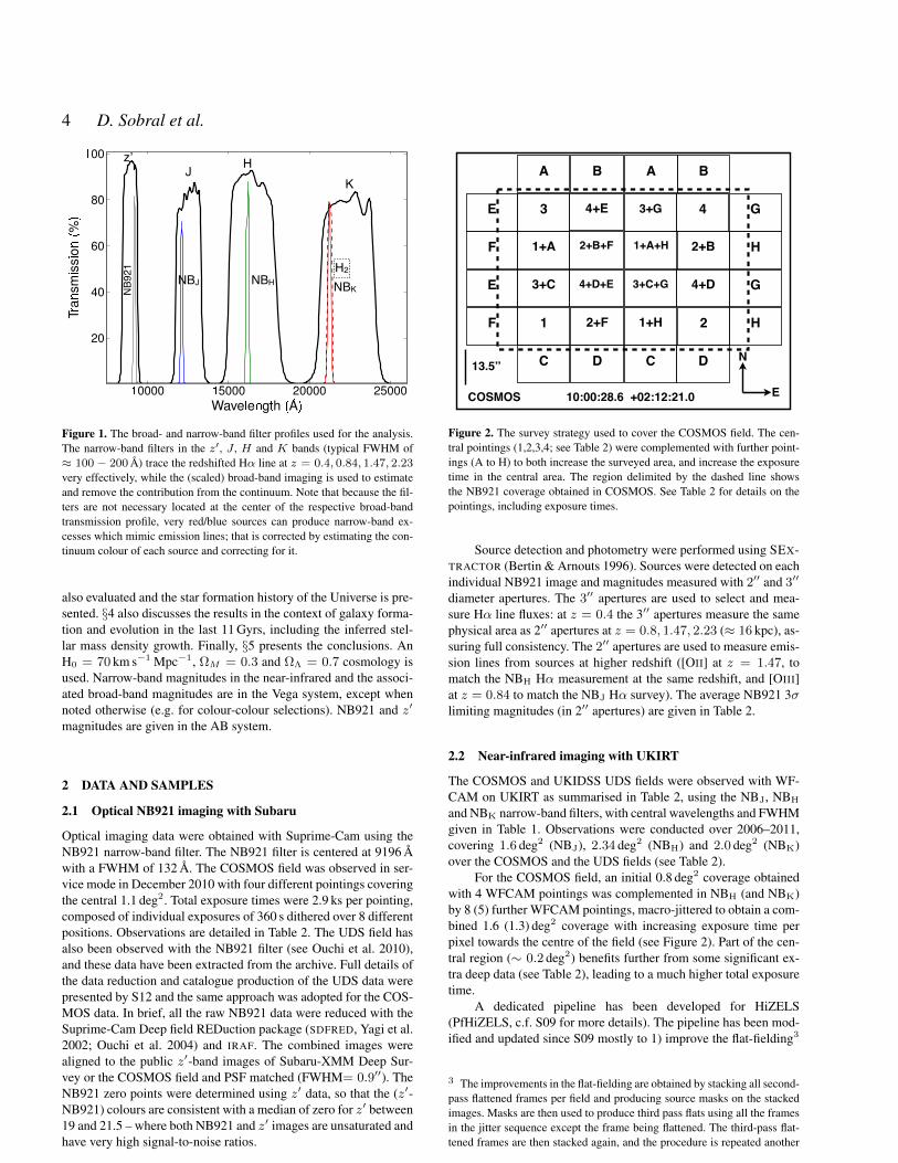
Figure 2. The survey strategy used to cover the COSMOS field. The cen-tral pointings (1,2,3,4; see Table 2) were complemented with further point-ings (A to H) to both increase the surveyed area, and increase the exposuretime in the central area. The region delimited by the dashed line showsthe NB921 coverage obtained in COSMOS. See Table 2 for details on thepointings, including exposure times.

Source detection and photometry were performed using SEX-TRACTOR (Bertin & Arnouts 1996). Sources were detected on eachindividual NB921 image and magnitudes measured with 2′′ and 3′′

diameter apertures. The 3′′ apertures are used to select and mea-sure Hα line fluxes: at z = 0.4 the 3′′ apertures measure the samephysical area as 2′′ apertures at z = 0.8, 1.47, 2.23 (≈ 16 kpc), as-suring full consistency. The 2′′ apertures are used to measure emis-sion lines from sources at higher redshift ([OII] at z = 1.47, tomatch the NBH Hα measurement at the same redshift, and [OIII]at z = 0.84 to match the NBJ Hα survey). The average NB921 3σlimiting magnitudes (in 2′′ apertures) are given in Table 2.

2.2 Near-infrared imaging with UKIRT

The COSMOS and UKIDSS UDS fields were observed with WF-CAM on UKIRT as summarised in Table 2, using the NBJ, NBH

and NBK narrow-band filters, with central wavelengths and FWHMgiven in Table 1. Observations were conducted over 2006–2011,covering 1.6 deg2 (NBJ), 2.34 deg2 (NBH) and 2.0 deg2 (NBK)over the COSMOS and the UDS fields (see Table 2).

For the COSMOS field, an initial 0.8 deg2 coverage obtainedwith 4 WFCAM pointings was complemented in NBH (and NBK)by 8 (5) further WFCAM pointings, macro-jittered to obtain a com-bined 1.6 (1.3) deg2 coverage with increasing exposure time perpixel towards the centre of the field (see Figure 2). Part of the cen-tral region (∼ 0.2 deg2) benefits further from some significant ex-tra deep data (see Table 2), leading to a much higher total exposuretime.

A dedicated pipeline has been developed for HiZELS(PfHiZELS, c.f. S09 for more details). The pipeline has been mod-ified and updated since S09 mostly to 1) improve the flat-fielding3

3 The improvements in the flat-fielding are obtained by stacking all second-pass flattened frames per field and producing source masks on the stackedimages. Masks are then used to produce third pass flats using all the framesin the jitter sequence except the frame being flattened. The third-pass flat-tened frames are then stacked again, and the procedure is repeated another

c© 2012 RAS, MNRAS 000, 1–18


and 2) provide more accurate astrometric solutions for each individ-ual frame which result in a more accurate stacking4. The updatedversion of the pipeline (PfHiZELS2012) has been used to reduce allUKIRT narrow band data (NBJ, NBH and NBK), including thosealready presented in previous papers. This approach guarantees acomplete self-consistency and takes advantage of the improved re-duction which, in some cases, is able to go deeper by ≈ 0.2 magwhen compared to the data reduced by the previous version of thepipeline.

For the COSMOS field, due to the need to co-add frames takenwith different WFCAM cameras (due to the survey strategy, seeFigure 2), IRAF is used to distort-correct all final frames (in addi-tion to individual frames being corrected prior to combining) beforeco-adding different fields; the typical rms is 0.1−0.2′′. However, atthe highest radial distances (r > 1000 pix) from the centre of theimages, even small residual distortions (sometimes with oppositesigns due to the need of combining different WFCAM cameras)can lead to an elongated PSF and blurring of sources. The com-bined frames were analysed using IRAF and it was found that forr < 900 (pix, from the centre of the images obtained with differentWFCAMs) the PSF/ellipticity remained unchanged due to stack-ing, but that for higher radial distances the PSF became increas-ingly elongated, particularly in the corners. In order to avoid intro-ducing errors in the photometry and source position, regions withoverlapping WFCAM cameras are treated in the following way: i)for r < 900 pix, the stacked images are used and ii) for r > 900pix the deepest individual image is used.

Narrow-band images were photometrically calibrated (inde-pendently) by matching ∼ 100 stars per frame with J , H and Kbetween the 12th an 16th magnitudes from the 2MASS All-Skycatalogue of Point Sources (Cutri et al. 2003) which are unsat-urated in the narrow-band images. WFCAM images are affectedby cross-talk and other artifacts caused by bright stars: accuratemasks are produced in order to reject such regions. Sources wereextracted using SEXTRACTOR (Bertin & Arnouts 1996), makinguse of the masks. Photometry was measured in apertures of 2′′ di-ameter which at z = 0.8 − 2.2 recover Hα fluxes over ≈ 16 kpc.The average 3σ depths of the entire set of NB frames vary signifi-cantly, and are summarised in Table 2. The total numbers of sourcesdetected with each filter are given in Table 3.

2.3 Near-infrared H2 imaging with HAWK-I

The UKIDSS UDS and COSMOS fields were observed with theHAWK-I instrument (Pirard et al. 2004; Casali et al. 2006) on theVLT during 2009. A single dithered pointing was obtained in eachof the fields using the H2 filter, characterised by λc = 2.124µmand δλ = 0.030µm (note that the filter is slightly wider than thaton WFCAM). Individual exposures were of 60 s, and the total ex-posure time per field is 5 hours. Table 2 presents the details of theobservations and depth reached.

Data were reduced using the HAWK-I ESO pipeline recipes,by following an identical reduction scheme/procedure to the WF-CAM data. The data have also been distortion corrected and as-trometrically calibrated before combining, using the appropriate

time. This procedure is able to both mask many sources which are unde-tected in individual frames out of the flats, but particularly to mask brightsources much more effectively, as the stacking of all images reveals a widerdistribution of flux from those sources.4 IRAF is used to distort correct the frames and obtain the best astrometricsolution for each frame, always assuring that the flux is conserved.

pipeline recipes. After combining all the individual reduced framesit is possible to obtain a contiguous image of ≈ 7.5 × 7.5 arcmin2 in each of the fields. There are, nonetheless, small regionswith slightly lower exposure time per pixel in regions related withchip gaps at certain positions. Because of the availability of thevery wide WFCAM imaging, regions in the HAWK-I combinedimages for which the exposure time per pixel is < 80% of the to-tal are not considered. Frames are photometrically calibrated using2MASS as a first pass, and then using UDS and COSMOS Ks cal-ibrated images to guarantee a median 0 colour (K-NBK ) for allmagnitudes probed, as this procedure provides a larger number ofsources. Similarly to the procedure used for WFCAM data, sourceswere extracted using SEXTRACTOR and photometry was measuredin apertures of 2′′ diameter.

2.4 Narrowband excess selection

In order to select potential line emitters, broad-band (BB) imag-ing is used in the z′, J , H and Ks bands to match narrow-band(NB) imaging in the NB921, NBJ, NBH and NBK/H2, respec-tively. Count levels on the broad-band images are scaled down tomatch the counts (of 2MASS sources) for each respective narrow-band image, in order to guarantee a median zero colour, and a com-mon counts-to-magnitude zero point. Sources are extracted fromBB images using the same aperture sizes used for NB imagesand matched to the NB catalogue with a search radius of < 0.9′′.Note, however, that none of the narrow-band filters fall at the centreof the broad-band filters (see Figure 1). Thus, objects with signifi-cant continuum colours will not have BB −NB = 0; this can becorrected with broad-band colours (c.f. S12), in order to guaranteethat BB−NB distribution is centred on 0 and has no dependenceon continuum broad-band colours. Average colour corrections5 aregiven by:

(z′−NB921)AB = (z′−NB921)0,AB−0.05(JAB−z′AB)−0.04

(J−NBJ) = (J−NBJ)0 − 0.09(z′AB − JAB) + 0.11

(H−NBH) = (H−NBH)0 + 0.07(JAB −HAB) + 0.06

(K−NBK) = (K−NBK)0 − 0.02(HAB −KAB) + 0.04

Potential line emitters are then selected according to the sig-nificance of their (BB − NB) colour, as they will have (BB −NB) > 0. True emitters are distinguished from those with positivecolours due to the scatter in the magnitude measurements by quan-tifying the significance of the narrowband excess. The parameter Σ(see Bunker et al. 1995) quantifies the excess compared to the ran-dom scatter expected for a source with zero colour, as a function ofnarrow-band magnitude (see e.g. S09), and is given by:

Σ =1− 10−0.4(BB−NB)

10−0.4(ZP−NB)√πr2

ap(σ2NB + σ2

BB), (1)

where ZP is the zero point of theNB (andBB, as those have beenscaled to have the same ZP as NB images), rap is the apertureradius (in pixels) used, and σNB and σBB are the rms (per pixel) ofthe NB and BB images, respectively.

Here, potential line emitters are selected if Σ > 3.0. Thespread on the brighter end (narrow-band magnitudes which are notsaturated, but for which the scatter is not affected by errors in the

5 Sources for which one of the broad-band colours is not available are as-signed the median correction. The median corrections are: −0.04, +0.07,+0.05 and +0.03 for NB921, NBJ, NBH and NBK respectively.

c© 2012 RAS, MNRAS 000, 1–18

6 D. Sobral et al.

NB921 NBJ

NBH NBK

Hα

Hα Hα

Hα Hß [OIII]

[OII]

Hß [OIII]

Hß [OIII]

Paα Paß

Hß [OIII]

[OII]

HeI [SIII]

Figure 3. Photometric redshift distributions (peak of the probability distribution function for each source) for the NB921 line emitter candidates (upper left).NBJ (upper right), NBH (lower left) and NBK (lower right). All distributions peak at redshifts which correspond to strong emission lines, corresponding toHα, Hβ, [OIII] and [OII] emitters at various redshifts depending on the central wavelength of each narrow-band filter. Other populations of emitters are alsofound, such as Paschen-lines. The dotted lines indicate the redshift for which an emission line is detectable by the narrow-band filters. Lyα emitter candidatesin the NB921 dataset (e.g. 18 sources in COSMOS) with photo-z of z ∼ 6− 7 are not shown.

magnitude, i.e., much brighter than the limit of the images) is quan-tified for each data-set and frame, and the minimum (BB −NB)colour limit over bright magnitudes is set by the 3× the standarddeviation of the excess colour over such magnitudes (sb). A com-mon rest-frame EW limit of EW0 = 25 A is applied, guaranteeing alimit higher than the 3×sb dispersion over bright magnitudes in allbands. The combined selection criteria guarantees a clean selectionof line emitters and, most importantly, it ensures that the samples ofHα emitters are selected down to the same rest-frame EW, allowingone to quantify the evolution across cosmic time.

As a further check on the selection criteria, the original imag-ing data are used to produce BB and NB postage stamp imagesof all the sources. The BB is subtracted from the NB image leav-ing the residual flux. From visual inspection these residual imagescontain obvious narrow band sources and it is found that the re-maining flux correlates well with the catalogue significance, withsignificance being proportional to residual flux (f ) asf (0.93±0.03).

2.5 The samples of NB line emitters

Narrow-band detections below the estimated 3σ detection thresh-old were not considered. By using colour-colour diagnostics (seeS12), potential stars are identified in the sample and rejected as well(the small fraction varies from band to band; see Table 3). The sam-ple of remaining potential emitters (Σ > 3 & EW0 > 25 A; see Ta-ble 3 for numbers) is visually checked to identify spurious sources,artifacts which might not have been masked, or sources being iden-tified in very noisy regions. Sources classed as spurious/artifacts areremoved from the sample of potential emitters. The final samplesof line emitters are then derived.

As a further test of the reliability of the line emitter samples, itcan be noted that since the HAWK-I observations are both deeperand obtained over a larger redshift slice (due to a wider filter pro-file) when compared to WFCAM, they should be able to confirmall NBK emitters over the matched area. This is confirmed, as all10 emitters which are detected with WFCAM in the matched areaare recovered by HAWK-I data as well.

The catalogues, containing all narrow-band emitter candi-dates, are presented in Appendix A. The catalogues provide IDs,coordinates, narrow-band and broad-band magnitudes, estimated

c© 2012 RAS, MNRAS 000, 1–18


fluxes and observed EWs. Further details and information are avail-able on the HiZELS website.

The photometric redshift (Photo-zs from Ilbert et al. 2009;Cirasuolo et al. 2010) distributions of the sources selectedwith the 4 narrow-band filters are presented in Figure 3. Thephotometric redshifts show clear peaks associated with Hα,Hβ/[OIII]λλ4959,5007, and [OII]λ3727 (see Figure 3), together withfurther emission lines such as Paschen lines and Lyα. Spectro-scopic redshift are also available for a fraction of the selected line-emitters (Lilly et al. 2009; Yamada et al. 2005; Simpson et al. 2006;Geach et al. 2008; van Breukelen et al. 2007; Ouchi et al. 2008;Smail et al. 2008; Ono et al. 2010)6.

2.6 Selecting Hα emitters

Samples of Hα emitters at the various redshifts are selected using acombination of broad-band colours (colour-colour selections) andphotometric redshifts (when available). Colour-colour separation ofemitters are different for each redshift, and for some redshifts twosets of colour-colour separations are used to reduce contaminationto a minimum. Additionally, spectroscopically confirmed sourcesare included, and sources confirmed to be other emission lines re-moved from the samples – but the reader should note that for allfour redshifts the number of z-included sources missed by the se-lection is typically < 10, while the z-rejected sources are typically< 10 as well. Therefore, the decrease of available spectroscopicredshifts with redshift does not introduce any bias.

Additionally, sources found to be line emitters in two (or three,for Hα emitters at z = 2.23) bands, making them strong Hα can-didates are also included in the samples, even if they have beenmissed by the colour-colour and photometric selection (although itis found that only very few real Hα sources are missed by the se-lection criteria). Table 3 provides the number of sources, includingspectroscopically confirmed ones for each field at each redshift.

2.6.1 Hα emitters at z = 0.4

The selection of Hα emitters at z = 0.4 is done using the BRiK(B − R vs i−K) colour-colour selection (see Figure 4 and S12).In addition, all sources for which 0.35 < zphot < 0.45 are alsoincluded in the sample. Spectroscopic redshifts (from zCOSMOS;Lilly et al. 2009) are available for 38 sources. Thirty six sources areconfirmed to be at z = 0.391 − 0.412, while 2 sources are [NII]emitters. This implies a very high completeness of the sample, anda contamination of ∼ 5 per cent over the entire sample. Contami-nants have been removed, and spectroscopic sources added. A totalof 1742 Hα emitters at z = 0.4 are selected.


Sources are selected to be Hα emitters at z = 0.84 if 0.75 <zphot < 0.95 or if they satisfy the BRiK (see Figure 4; S09)colour-colour selection for z ∼ 0.8 sources. Additionally, sourceswith 1.3 < zphot < 1.7 (likely Hβ/[OIII] z ≈ 1.4 emitters) and2.0 < zphot < 2.5 (likely z = 2.23 [OII] emitters) are removed tofurther reduce contamination from higher redshift emitters. Sourceswith spectroscopically confirmed redshifts are included and sources

6 See UKIDSS UDS website for a redshift compilation by O. Almaini andthe COSMOS data archive for the catalogues, spectra and information onthe various instruments and spectroscopic programmes.

with other spectroscopically confirmed lines are removed. In prac-tice, 6 Hα spectroscopic sources missed by the selection criteriaare introduced in the sample; 7 sources found in the sample arenot Hα – a mix of [SII], [NII] and [OIII] emitters. A total of 95sources are spectroscopically confirmed as Hα, while 237 sourcesare confirmed as dual Hα-[OIII] emitters.


Note that, as described in S12, the NBH filter can be combined withNB921 (probing the [OII] emission line), to provide very clean,complete surveys of z = 1.47 line emitters, as the filter profiles areextremely well-matched for a dual Hα-[OII] survey. By applyingthe dual narrow-band selection, a total of 346 Hα-[OII] emittersare robustly identified in COSMOS and UDS. However, the dualnarrow-band selection is only complete if the NB921 survey probesdown to [OII]/Hα ∼ 0.1 (c.f. S12), which is not the case for thedeepest NBH COSMOS coverage. Additionally, only the central1.1 deg2 region of the COSMOS field has been targeted with theNB921 filter.

In order to select Hα emitters in areas where the NB921 is notdeep enough to provide a complete selection, or where NB921 dataare not available, the following steps are taken. Sources are selectedif 1.35 < zphot < 1.55, or if they satisfy the z ∼ 1.5BzK (B−zvs. z−K) criteria defined in Figure 4, which is able to recover thebulk of the dual narrow-band emitters and sources with high qual-ity photometric redshifts of z ∼ 1.5. However, the z ∼ 1.5 BzKselection, although highly complete, is still contaminated by higherredshift emitters. In order to exclude likely higher redshift sourcesan additional ziK (i − z vs. z −K; see S12) colour-colour sepa-ration is used (see Figure 5), in combination with rejecting sourceswith zphot > 1.8.

The selection leads to a total sample of 515 robust Hα emittersat z = 1.47, by far the largest sample of Hα emitters at z ∼ 1.5.Comparing the double NB921 and NBH analysis with the colourand photo-z selection (for sources for which the NB921 data aredeep enough to detect [OII]) shows that the colour and photo-z se-lection by itself results in a contamination of ≈ 15 per cent, anda completeness of ≈ 85 per cent. However, as the double NB921and NBH analysis has been used wherever the data are availableand sufficiently deep, the contamination of the entire sample is es-timated to be lower (≈ 5 per cent), and the completeness higher(≈ 95 per cent).


As can be seen from the photometric redshift distribution in Fig-ure 3, the high quality photo-zs in the COSMOS and UDS fieldscan provide a powerful tool to select z = 2.23 sources. However,the sole use of the photometric redshifts can not result in clean,high completeness sample of z = 2.23 Hα emitters, not only be-cause reliable photometric redshifts are not available for 35 percent of the NBK emitters, at the faint end, but also because theerrors in the photometric redshifts will be much higher at z ∼ 2.2than at lower redshift (particularly as one is selecting star-forminggalaxies). Nevertheless, although spectroscopy only exists for a fewHα z = 2.23 sources (zCOSMOS and UDS compilation), doubleline detections between NBK and one of NBH ([OIII]) and/or NBJ

([OII]) allow the identification of 84 secure Hα emitters. These canbe used to optimise the selection criteria and estimate the complete-ness and contamination of the sample.

c© 2012 RAS, MNRAS 000, 1–18

8 D. Sobral et al.

Table 3. A summary of the number of sources, narrow-band emitters and Hα-selected emitters for the various surveys undertaken with different narrow-bandfilters. Fields are C: COSMOS, U: UDS. Volumes are presented in units of 104 Mpc3 and correspond to the total volumes probed; deeper pointings coverrelatively smaller volumes. SFRs (limiting SFRs) are presented uncorrected for dust extinction. The number of spectroscopically confirmed Hα emitters arepresented in the z Hα conf column, while the number of Hα sources which are confirmed by an emission-line detection in another narrow-band filter arepresented in Conf 2lines. Note that the SFR limits represent the limit over the deepest field(s). Also, note that for all four redshifts the number of z-includedsources missed by the selection is typically < 10, while the z-rejected sources are typically < 10 as well. Therefore, decrease of available spectroscopicredshifts with redshift does not introduce any bias.

Filter Field Detect W/ Colours Emitters Stars Spurious Hα z Hα conf. Conf 2lines Volume Hα SFRNB C/U 3σ # 3 Σ # # # # # 104 Mpc3 M yr−1

NB921 C 155542 148702 2885 (3066) 247 – 521 38 – 5.1 0.03NB921 U 236718 198256 5799 (6574) 775 – 1221 8 – 5.1 0.01

NBJ C 32345 31661 689 (773) 40 46 425 81 158 7.9 1.5NBJ U 21233 19916 497 (574) 49 30 212 14 79 11.1 1.5

NBH C 65912 64453 701 (818) 60 63 327 28 158 68.9 3.0NBH U 26084 23503 354 (382) 23 5 188 18 188 22.8 5.0

NBK C 65301 64008 754 (828) 54 23 346 4 65 31.2 7.0NBK U 28276 26062 360 (395) 32 10 172 2 19 22.4 10.0H2 C 1054 940 52 (57) 3 2 31 0 2 0.9 3.5H2 U 1193 1059 33 (41) 7 1 14 0 0 0.9 3.5

The selection of Hα emitters is done in the same way for bothCOSMOS and UDS, and for both WFCAM and HAWK-I data. Aninitial sample of z = 2.23 Hα emitters is obtained by selectingsources for which 1.7 < zphot < 2.8, where the limits were deter-mined using the distribution of photometric redshifts found for con-firmed Hα emitters at z = 2.23 (this selects 345 sources, of whichonly 2 are spectroscopically confirmed to be contaminants). Be-cause some sources lack reliable photometric redshifts, the colourselection (z−K) > (B−z) is used recover additional z ∼ 2 faintemitters. This colour-colour selection is a slightly modified versionof the standardBzK colour-colour separation (Daddi et al. 2004)7.It selects 307 additional Hα candidates (and re-selects 331 [96%]of those selected through photometric redshifts), and guarantees ahigh completeness of the Hα sample (see Figure 4). However, theBzK selection also selects z ∼ 3.3 Hβ/[OIII] emitters very ef-fectively, and the contamination by such emitters needs to be min-imised. In order to do this, sources with zphot > 3.0 are excluded(64 sources). For sources for which a photometric redshift does notexist, a rest-frame UV colour-colour separation is used (B −R vs.U−B; see Figure 5, probing the rest-frame UV), capable of broadlyseparating z = 2.23 and z ∼ 3.3 emitters due to their different UVcolours (see Figure 5; this removes a further 29 sources). Four fur-ther sources are removed as they are confirmed contaminants (amix of Paβ, [SIII] and [OIII] at z = 0.65, z = 1.23 and z = 3.23,respectively).

Overall, the selection leads to a total sample of 556 Hα emit-ters, by far the largest sample of z = 2.23 Hα emitters, and anorder of magnitude larger than the previous largest samples pre-sented by Geach et al. (2008) and Hayes et al. (2010). With thelimited spectroscopy available, it is difficult to accurately determinethe completeness and contamination of the sample, but based on the

7 The selection was modified because the Daddi et al. cut was designed toselect z > 1.4 sources, while here z = 2.23 emitters are targeted. Theprecise location of the new cut, which is 0.2 magnitudes higher than that ofDaddi et al., is motivated by the confirmed Hα emitters, and all of them arerecovered by the modified cut).

double-line detections the completeness is estimated to be> 90 percent, and contamination is likely to be ≈ 10 per cent.

3 ANALYSIS AND RESULTS: Hα LF OVER 11 GYRS

3.1 Removing the contamination by the [NII] line

Due to the width of all filters in detecting the Hα line, the ad-jacent [NII] lines can also be detected when the Hα line is de-tected at the peak transmission of the filter. A correction for the[NII] line contamination is therefore done, following the rela-tion given in S12. The relation has been derived to reproducethe full SDSS relation between the average log([NII]/Hα), f , andlog[EW0([NII]+Hα)], E: f = −0.924 + 4.802E − 8.892E2 +6.701E3 − 2.27E4 + 0.279E5. This relation is used to correct allHα fluxes at z = 0.4, 0.84, 1.47 and 2.23. The median correction(the median [NII]/([NII]+Hα)) is ≈ 0.25.

3.2 Completeness corrections: detection and selection

It is fundamental to understand how complete the samples are as afunction of line flux. This is done using simulations, as described inS09 and further detailed in S12. The simulations consider two ma-jor components driving the incompleteness: i) the detection com-pleteness (which depends on the actual imaging depth and the aper-tures used) and ii) the incompleteness resulting from the selection(both EW and colour significance).

The detection completeness is estimated by placing sourceswith a given magnitude at random positions on each individualnarrow-band image, and studying the recovery rate as a functionof the magnitude of the source. For the large Subaru frames, 2500sources are added for each magnitude, for WFCAM images 500,and for HAWK-I frames 100 sources are added for each realisa-tion.

The individual line completeness estimates are performed inthe same way for the data at the four different redshifts. A set ofgalaxies is defined, which is consistent with being at the approx-imate redshift (applying the same photometric redshift + colour-

c© 2012 RAS, MNRAS 000, 1–18


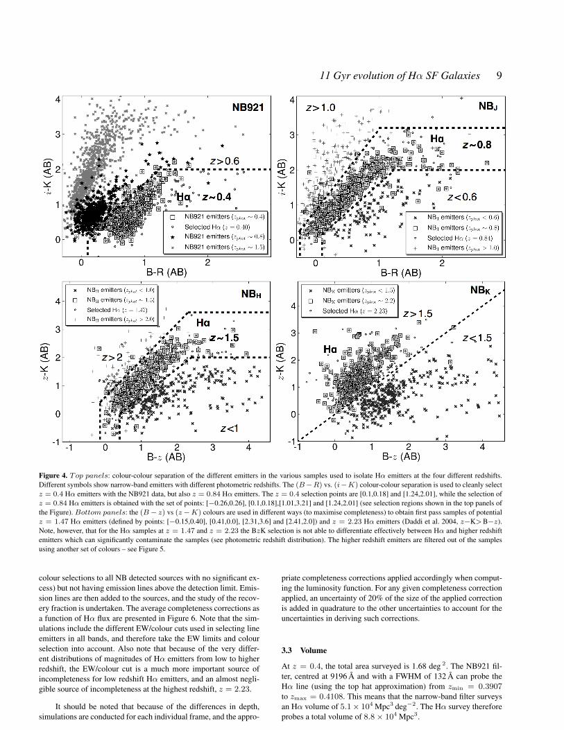
Figure 4. Top panels: colour-colour separation of the different emitters in the various samples used to isolate Hα emitters at the four different redshifts.Different symbols show narrow-band emitters with different photometric redshifts. The (B−R) vs. (i−K) colour-colour separation is used to cleanly selectz = 0.4 Hα emitters with the NB921 data, but also z = 0.84 Hα emitters. The z = 0.4 selection points are [0.1,0.18] and [1.24,2.01], while the selection ofz = 0.84 Hα emitters is obtained with the set of points: [−0.26,0.26], [0.1,0.18],[1.01,3.21] and [1.24,2.01] (see selection regions shown in the top panels ofthe Figure). Bottom panels: the (B− z) vs (z−K) colours are used in different ways (to maximise completeness) to obtain first pass samples of potentialz = 1.47 Hα emitters (defined by points: [−0.15,0.40], [0.41,0.0], [2.31,3.6] and [2.41,2.0]) and z = 2.23 Hα emitters (Daddi et al. 2004, z−K>B−z).Note, however, that for the Hα samples at z = 1.47 and z = 2.23 the BzK selection is not able to differentiate effectively between Hα and higher redshiftemitters which can significantly contaminate the samples (see photometric redshift distribution). The higher redshift emitters are filtered out of the samplesusing another set of colours – see Figure 5.

colour selections to all NB detected sources with no significant ex-cess) but not having emission lines above the detection limit. Emis-sion lines are then added to the sources, and the study of the recov-ery fraction is undertaken. The average completeness corrections asa function of Hα flux are presented in Figure 6. Note that the sim-ulations include the different EW/colour cuts used in selecting lineemitters in all bands, and therefore take the EW limits and colourselection into account. Also note that because of the very differ-ent distributions of magnitudes of Hα emitters from low to higherredshift, the EW/colour cut is a much more important source ofincompleteness for low redshift Hα emitters, and an almost negli-gible source of incompleteness at the highest redshift, z = 2.23.

It should be noted that because of the differences in depth,simulations are conducted for each individual frame, and the appro-

priate completeness corrections applied accordingly when comput-ing the luminosity function. For any given completeness correctionapplied, an uncertainty of 20% of the size of the applied correctionis added in quadrature to the other uncertainties to account for theuncertainties in deriving such corrections.

3.3 Volume

At z = 0.4, the total area surveyed is 1.68 deg 2. The NB921 fil-ter, centred at 9196 A and with a FWHM of 132 A can probe theHα line (using the top hat approximation) from zmin = 0.3907to zmax = 0.4108. This means that the narrow-band filter surveysan Hα volume of 5.1× 104 Mpc3 deg−2. The Hα survey thereforeprobes a total volume of 8.8× 104 Mpc3.

c© 2012 RAS, MNRAS 000, 1–18

10 D. Sobral et al.

z~2.3Hß/[OIII]

z=1.47Hα

z=2.23Hα

z~3.3Hß/[OIII]

Figure 5. Top: Colour-colour separation of z = 1.47 Hα emitters andthose at higher redshift (z ∼ 2.3 Hβ/[OIII], z ∼ 3.3 [OII]); separation isobtained by (z−K) < 5(i−z)−0.4.Bottom: colour-colour separation ofz ∼ 3 Hβ/[OIII] emitters from z = 2.23 Hα emitters, given by (B−R) <

−0.55(U−B)+1.25. Using the BzK colour-colour separation only resultsin some contamination of the Hα sample with higher redshift emitters –the B − R vs U − B colour-colour separation allows to greatly reducethat. The Figure also indicates the location of each final Hα selected sourcein the colour-colour plot. Note that sources shown as zphot ∼ 1.5 andzphot ∼ 2.2 are those with photometric redshifts which are within ±0.2

of those values.

The NBJ filter (FWHM of 140 A) can be approximated by atop hat, probing zmin = 0.8346 to zmax = 0.8559 for Hα linedetections, resulting in surveying 1.5 × 105 Mpc3 deg−1. As thetotal survey has covered 1.3 deg2, it results in a total volume of1.9 × 105 Mpc3. Assuming the top hat (TH) model for the NBH

filter (FWHM of 211.1 A, with λTHmin = 1.606µm and λTHmax =1.627µm), the Hα survey probes a (co-moving) volume of 3.3 ×105 Mpc3 deg−2. Volumes are computed on a field by field basisas each field reaches a different depth (although the difference involume is only important at the faintest fluxes). The total volumeof the survey is 7.4 × 105 Mpc3. The volume down to the deepestdepth is 3.9× 104 Mpc3 (see Table 4 for details). The NBK filter iscentred on λ = 2.121µm, with a FWHM of 210 A. Using the tophat approximation for the filter, it can probe the Hα emission linefrom zmin = 2.2147 to zmax = 2.2467, so with a ∆z = 0.016.The H2 filter therefore probes a volume of 3.8× 105 Mpc3 deg−2.

The HAWK-I survey uses a slightly different H2 filter, cen-tred on λ = 2.125µm, with FWHM = 300 A. A top hat is an even

Figure 6. Average completeness of the various narrow-band surveys as afunction of Hα flux. Note that the completeness of individual fields/framesfor each band can vary significantly due to the survey strategy (e.g. seedifference between one of the deep pointings in COSMOS, NBH D andthe average over all NBH fields), and thus the completeness corrections arecomputed for each individual fields.

better approximation of the filter profile, with zmin = 2.2139 tozmax = 2.2596 for Hα line detections. The filter effectively probes5.5× 105 Mpc3 deg−2. Each HAWK-I pointing covers only about13.08 arcmin2, and so the complete HAWK-I survey (COSMOSand UDS, 0.0156 deg2) probes a total volume of 1.7 × 104 Mpc3.Note that the survey conducted by Hayes et al. (2010) (using a nar-rower NB filter), although deeper, only probed 5.0 × 103 Mpc3,so a factor of 3 smaller in volume and over a single field. Table4 presents a summary of the volumes probed as a function of Hαluminosity and the number of sources detected at each redshift.

3.4 Filter Profiles: volume corrections

None of the narrow band filters are perfect top hats (see Figure1). In order to model the effect of this bias on estimating the vol-ume (luminous emitters will be detectable over larger volumes –although, if seen in the filter wings, they will be detected as fainteremitters), a series of simulations is done, following S09 and S12.Briefly, a top hat volume selection is used to compute a first-pass(input) luminosity function and derive the best fit. The fit is used togenerate a population of simulated Hα emitters (assuming they aredistributed uniformly across redshift); these are then folded throughthe true filter profile, from which a recovered luminosity function isdetermined. Studying the difference between the input and recov-ered luminosity functions shows that the number of bright emit-ters is underestimated, while faint emitters can be slightly overesti-mated (c.f. S09 for details), but the actual corrections are differentfor each filter and each input luminosity function. This allows cor-rection factors to be estimated – these are then used to obtain thecorrected luminosity function. Corrections are computed for eachindividual narrow-band filter.

3.5 Extinction Correction

The Hα emission line is not immune to dust extinction. Measur-ing the extinction for each source can in principle be done by sev-eral methods, one of which is the comparison between Hα and far-

c© 2012 RAS, MNRAS 000, 1–18


infrared determined SFRs (see Ibar et al. in prep.), while the spec-troscopic analysis of Balmer decrements also provides a very goodestimate of the extinction. As shown in S12, the [OII]/Hα line ratiocan also be reasonably well calibrated (using Balmer decrement)as a dust extinction indicator. For the COSMOS z = 1.47 sample,this results in AHα = 0.8 mag (although there is a bias towardslower extinction due to the fact that the NB921 survey is not deepenough to recover sources with much higher extinctions). However,for UDS (where a sufficiently deep NB921 coverage is available)a AHα ≈ 1 mag of extinction at Hα is shown to be an appropri-ate median correction at z = 1.47 (see S12). That is also similarhas been found at z = 0.84 (Garn et al. 2010, AHα ≈ 1.2). Thedependence of extinction on observed luminosity is also relativelysmall (S12) at z ∼ 1.5 – therefore, for simplicity and for an easiercomparison, a simple 1 mag of extinction is applied for the fourredshifts and for all observed luminosities. Note that S12 still finda relatively mild luminosity dependence, but one which is offset tothe local Universe relation (e.g. Hopkins et al. 2001) by 0.5 mag inAHα (or, alternatively, the relation is not offset once luminositiesare divided by L∗Hα at that epoch and compared with local lumi-nosities divided by the local L∗Hα).

3.6 Hα Luminosity Functions at z = 0.40,0.84,1.47,2.23

By taking all Hα selected emitters at the four different redshifts,the Hα luminosity function is computed at 4 very different cos-mic times, reaching a common observed luminosity limit of ≈1041.6 erg s−1 for the first time in a consistent way over∼ 11 Gyrs.As previously described, the method of S09 and S12 is applied tocorrect for the real profile (see Section 3.4). Candidate Hα emittersare assumed to be at z = 0.4, 0.84, 1.47 and 2.23 for luminositydistance calculations. Results can be found in Figure 7 and Table4. Errors are Poissonian, but they include a further 20% of the totalcompleteness corrections added in quadrature.

All derived luminosity functions are fitted with Schechterfunctions defined by three parameters α, φ∗ and L∗:

φ(L)dL = φ∗(

L

L∗

)αe−(L/L∗)d

(L

L∗

), (2)

which are found to provide good fits to the data at all redshifts. Inthe log form, the Schechter function is given by:

φ(L)dL = ln 10φ∗(

L

L∗

)αe−(L/L∗)

(L

L∗

)d log L. (3)

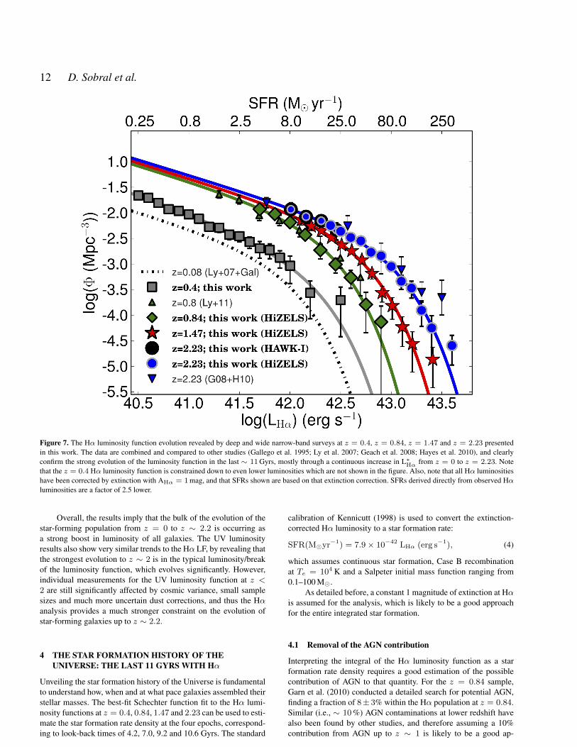
Schechter functions are fitted to each luminosity function. The bestfits for the Hα luminosity functions at z = 0.4 − 2.23 are pre-sented in Table 5, together with the uncertainties on the parame-ters (1σ). Uncertainties are obtained from either the 1σ deviationfrom the best-fit, or the 1σ variance of fits, obtained with a suite ofmultiple luminosity functions with different binning – whichever ishigher (although they are typically comparable). The best-fit func-tions and their errors are also shown in Figure 7, together with thez ≈ 0 luminosity function determined by Ly et al. (2007) – whichhas extended the work by Gallego et al. (1995) at z ≈ 0, for alocal-Universe comparison. Deeper data from the literature are alsopresented for comparison; Ly et al. (2011) for z = 0.8, and Hayeset al. (2010) for z = 2.23, after applying the small corrections toensure the extinction corrections are consistent8.

The results not only reveal a very clear evolution of the Hα

8 The correction is applied to obtain data points corrected for extinction by1 mag at Hα.

luminosity function from z = 0 to z = 2.23, but they also allowfor a detailed investigation of exactly how the evolution occurs, insteps of ∼ 2 − 3 Gyrs. The strongest evolutionary feature is theincrease in L∗Hα as a function of redshift from z = 0 to z = 2.23(see Figure 8), with the typical Hα luminosity at z ∼ 2 (L∗Hα)being 10 times higher than locally. This is clearly demonstratedin Figure 8, which shows the evolution of the Schechter functionparameters describing the Hα luminosity function. The L∗Hα evo-lution from z ∼ 0 to z ∼ 2.2, can be simply approximated aslog L∗ = 0.45z + log L∗z=0, with log L∗z=0 = 41.87 (see Figure8). At the very bright end (L > 4L∗), and particularly at z > 1,there seems to be a deviation from a Schechter function. Follow-upspectroscopy of such luminous Hα sources has recently been ob-tained for a subset of the z = 1.47 sample, and unveil a significantfraction of narrow and broad-line AGN (with strong [NII] lines aswell) which become dominant at the highest luminosities (Sobral etal. in prep). It is therefore likely that the deviation from a Schechterfunction is being mostly driven by the increase in the AGN activ-ity fraction at such luminosities, particularly due to the detection ofrare broad-line AGN and from very strong [NII] emission.

The normalisation of the Hα luminosity function, φ∗, is alsofound to evolve, but much more mildly. There is an increase of φ∗

up to z ∼ 1 (by a factor ∼ 4), and then this decreases again forhigher redshifts by a factor of ∼ 2 from z ∼ 1 to z = 2.23 – seeFigure 8.

The faint-end slope, α, is found to be relatively steep fromz ∼ 0 up to z = 2.23 (when compared to a canonical α = −1.35),and it is not found to evolve. The median α over 0 < z < 2.23 is−1.60±0.08. Very deep data from Hayes et al. (2010) and Ly et al.(2011) not only agree well with such faint-end slope, but even moreimportantly, their data at the faintest luminosities are also very wellfitted by the best-fit z = 2.23 and z = 0.84 luminosity func-tions, even though their data points were not used for the fit. Itis therefore shown that by measuring the Hα luminosity functionin a consistent way, and using multiple fields, the faint-end slopecan be very well approximated by a constant α = −1.6 at leastup to z = 2.23. This shows that while the faint-end slope trulyis steep at z ∼ 2, it does not become significantly steeper fromz ∼ 0 to z ∼ 2, and rather has remained relatively constant for thelast 11 Gyrs. The potential steepening of the faint-end slope, whichhas been previously reported (e.g. Hayes et al. 2010) simply resultsfrom comparing different data-sets which probe different ranges inluminosity, use different completeness corrections, different selec-tion of emitters and probe a different parameter space. Furthermore,the results from Sobral et al. (2011) show that the faint-end slopedepends relatively strongly on environment, which indicates thatthe changes in the faint-end slope measured before may also haveresulted by the relatively small areas which can (by chance) probedifferent environments. Note that this is not the case for this pa-per because the multi-epoch Hα surveys cover∼ 2 deg2 areas overtwo independent fields and are therefore covering a wide range ofenvironments.

The steep faint-end slope of the Hα luminosity function is invery good agreement with the UV luminosity function at z ∼ 2 andabove, and particularly consistent with a relatively non-evolvingα ≈ −1.6. This can be seen by comparing the results in thispaper with those presented by Treyer et al. (1998), Arnouts et al.(2005), and more recently, Oesch et al. (2010). It is also likely that(similarly to the Hα luminosity function) the large scatter, and thedifferent selections/corrections applied, have driven studies to as-sume/argue for a steepening of the UV luminosity faint-end slope,just like for the Hα luminosity function – see Oesch et al. (2010).

c© 2012 RAS, MNRAS 000, 1–18

12 D. Sobral et al.

Figure 7. The Hα luminosity function evolution revealed by deep and wide narrow-band surveys at z = 0.4, z = 0.84, z = 1.47 and z = 2.23 presentedin this work. The data are combined and compared to other studies (Gallego et al. 1995; Ly et al. 2007; Geach et al. 2008; Hayes et al. 2010), and clearlyconfirm the strong evolution of the luminosity function in the last ∼ 11 Gyrs, mostly through a continuous increase in L∗Hα from z = 0 to z = 2.23. Notethat the z = 0.4 Hα luminosity function is constrained down to even lower luminosities which are not shown in the figure. Also, note that all Hα luminositieshave been corrected by extinction with AHα = 1 mag, and that SFRs shown are based on that extinction correction. SFRs derived directly from observed Hαluminosities are a factor of 2.5 lower.

Overall, the results imply that the bulk of the evolution of thestar-forming population from z = 0 to z ∼ 2.2 is occurring asa strong boost in luminosity of all galaxies. The UV luminosityresults also show very similar trends to the Hα LF, by revealing thatthe strongest evolution to z ∼ 2 is in the typical luminosity/breakof the luminosity function, which evolves significantly. However,individual measurements for the UV luminosity function at z <2 are still significantly affected by cosmic variance, small samplesizes and much more uncertain dust corrections, and thus the Hαanalysis provides a much stronger constraint on the evolution ofstar-forming galaxies up to z ∼ 2.2.

4 THE STAR FORMATION HISTORY OF THEUNIVERSE: THE LAST 11 GYRS WITH Hα

Unveiling the star formation history of the Universe is fundamentalto understand how, when and at what pace galaxies assembled theirstellar masses. The best-fit Schechter function fit to the Hα lumi-nosity functions at z = 0.4, 0.84, 1.47 and 2.23 can be used to esti-mate the star formation rate density at the four epochs, correspond-ing to look-back times of 4.2, 7.0, 9.2 and 10.6 Gyrs. The standard

calibration of Kennicutt (1998) is used to convert the extinction-corrected Hα luminosity to a star formation rate:

SFR(Myr−1) = 7.9× 10−42 LHα (erg s−1), (4)

which assumes continuous star formation, Case B recombinationat Te = 104 K and a Salpeter initial mass function ranging from0.1–100 M.

As detailed before, a constant 1 magnitude of extinction at Hαis assumed for the analysis, which is likely to be a good approachfor the entire integrated star formation.

4.1 Removal of the AGN contribution

Interpreting the integral of the Hα luminosity function as a starformation rate density requires a good estimation of the possiblecontribution of AGN to that quantity. For the z = 0.84 sample,Garn et al. (2010) conducted a detailed search for potential AGN,finding a fraction of 8± 3% within the Hα population at z = 0.84.Similar (i.e., ∼ 10 %) AGN contaminations at lower redshift havealso been found by other studies, and therefore assuming a 10%contribution from AGN up to z ∼ 1 is likely to be a good ap-

c© 2012 RAS, MNRAS 000, 1–18


α = -1.6

z=0.4

z=0.84z=1.47

z=2.23

Figure 8. The evolution of the Schechter function parameters which best fit the Hα luminosity function since z = 2.23. Top left: the evolution of L∗Hαas a function of redshift, revealing that the break of the luminosity function evolves significantly from z = 0 to z = 2.23 by a factor of 10, which can besimply parameterised by log L∗Hα = 0.45z + 41.87. Top right: the evolution of φ∗, which seems to rise mildly up to z ∼ 1 and decrease again up toz ∼ 2.2.Bottom left: the faint end slope, however, is not found to evolve at all from z = 0.0 to z = 2.23 within the scatter and the errors, pointing towardsα = −1.60± 0.08 for the faint-end slope of the Hα luminosity function across the last 11 Gyrs. Bottom right: The 1, 2 and 3σ contours of the best fits tothe combination of L∗Hα and φ∗ fixing α = −1.6.

Table 5. The luminosity function and star formation rate density evolution for 0.4 < z < 2.2, as seen through a completely self-consistent analysis usingHiZELS. The measurements are obtained at z = 0.4, 0.84, 1.47 and 2.23, correcting for 1 mag extinction at Hα. Columns present the redshift, break of theluminosity function, L∗Hα, normalisation (φ∗Hα) and faint-end slope (α) of the Hα luminosity function. The two right columns present the star formation ratedensity at each redshift based on integrating the luminosity function down to ≈ 3 M yr−1 or 41.6 (in log erg s−1) and for a full integration. Star formationrate densities include a correction for AGN contamination of 10% at z = 0.4 and z = 0.84 (see Garn et al. 2010) and 15% at both z = 1.47 and z = 2.23.Errors on the faint-end slope α are the 1σ deviation from the best fit, when fitting the 3 parameters simultaneously. As α is very well-constrained at allredshifts, and shown not to evolve significantly, L∗Hα and φ∗Hα are obtained by fixing α = −1.6, and the 1σ errors on L∗Hα and φ∗Hα are derived from suchfits (with fixed α).

Epoch L∗Hα φ∗Hα αHα log ρLHα41.6 log ρLHα

ρSFRHα 41.6 ρSFRHα All(z) erg s−1 Mpc−3 erg s−1 Mpc−3 erg s−1 Mpc−3 M yr−1 Mpc−3 M yr−1 Mpc−3

z = 0.40± 0.01 42.09+0.47−0.12 −3.12+0.10

−0.34 −1.75+0.12−0.08 38.99+0.19

−0.22 39.55+0.22−0.22 0.008+0.002

−0.002 0.03+0.01−0.01

z = 0.84± 0.02 42.25+0.07−0.05 −2.47+0.07

−0.08 −1.56+0.13−0.25 39.75+0.12

−0.05 40.13+0.24−0.21 0.040+0.007

−0.006 0.10+0.01−0.02

z = 1.47± 0.02 42.56+0.06−0.05 −2.61+0.08

−0.09 −1.62+0.25−0.29 40.03+0.08

−0.07 40.29+0.16−0.14 0.07+0.01

−0.01 0.13+0.02−0.02

z = 2.23± 0.02 42.86+0.10−0.07 −2.73+0.10

−0.12 −1.57+0.18−0.23 40.29+0.04

−0.04 40.47+0.06−0.06 0.13+0.01

−0.01 0.20+0.03−0.04

c© 2012 RAS, MNRAS 000, 1–18

14 D. Sobral et al.

Table 4. Luminosity Functions from HiZELS. LHα has been corrected forboth [NII] contamination and for dust extinction (using AHα = 1 mag).

logLHα Sources φ obs φ corr Volume

z = 0.40 # Mpc−3 Mpc−3 104 Mpc3

40.50± 0.05 128 −1.84± 0.04 −1.66± 0.04 8.840.60± 0.05 147 −1.78± 0.04 −1.70± 0.04 8.840.70± 0.05 118 −1.87± 0.04 −1.81± 0.04 8.840.80± 0.05 86 −2.01± 0.05 −1.93± 0.05 8.840.90± 0.05 56 −2.20± 0.06 −1.96± 0.07 8.841.00± 0.05 54 −2.21± 0.06 −2.03± 0.07 8.841.10± 0.05 34 −2.41± 0.08 −2.12± 0.09 8.841.20± 0.05 36 −2.39± 0.08 −2.27± 0.08 8.841.30± 0.05 33 −2.43± 0.08 −2.29± 0.09 8.841.40± 0.05 25 −2.55± 0.10 −2.42± 0.10 8.841.50± 0.05 25 −2.55± 0.10 −2.46± 0.11 8.841.60± 0.05 17 −2.71± 0.12 −2.57± 0.13 8.841.70± 0.05 10 −2.94± 0.17 −2.69± 0.19 8.841.80± 0.05 11 −2.90± 0.16 −2.73± 0.17 8.841.90± 0.05 8 −3.04± 0.19 −2.88± 0.20 8.842.00± 0.05 4 −3.34± 0.30 −3.03± 0.35 8.842.20± 0.10 3 −3.45± 0.36 −3.56± 0.51 8.842.50± 0.15 2 −3.64± 0.53 −3.71± 0.71 8.8

z = 0.84 # Mpc−3 Mpc−3 104 Mpc3

41.70± 0.075 218 −2.12± 0.03 −1.93± 0.03 19.141.85± 0.075 222 −2.11± 0.03 −2.02± 0.03 19.142.00± 0.075 107 −2.43± 0.04 −2.18± 0.04 19.142.15± 0.075 54 −2.72± 0.06 −2.43± 0.06 19.142.30± 0.075 12 −3.38± 0.15 −2.73± 0.17 19.142.45± 0.075 10 −3.46± 0.17 −3.01± 0.17 19.142.60± 0.075 7 −3.61± 0.21 −3.27± 0.21 19.142.75± 0.075 2 −4.16± 0.53 −3.79± 0.55 19.142.90± 0.075 1 −4.46± 0.90 −4.13± 1.51 19.1

z = 1.47 # Mpc−3 Mpc−3 104 Mpc3

42.10± 0.05 25 −2.20± 0.10 −2.13± 0.10 4.042.20± 0.05 32 −2.37± 0.08 −2.25± 0.09 7.542.30± 0.05 62 −2.55± 0.06 −2.34± 0.06 22.142.40± 0.05 86 −2.67± 0.05 −2.47± 0.05 40.242.50± 0.05 101 −2.78± 0.05 −2.62± 0.05 60.442.60± 0.05 106 −2.83± 0.04 −2.73± 0.04 71.442.70± 0.05 43 −3.23± 0.07 −2.91± 0.08 73.642.80± 0.05 23 −3.50± 0.10 −3.18± 0.11 73.642.90± 0.05 9 −3.91± 0.18 −3.55± 0.18 73.643.00± 0.05 5 −4.17± 0.26 −3.81± 0.26 73.643.10± 0.05 3 −4.39± 0.37 −4.22± 0.38 73.643.20± 0.05 2 −4.57± 0.53 −4.55± 0.55 73.643.40± 0.15 2 −4.57± 0.53 −4.86± 0.55 73.6

z = 2.23 # Mpc−3 Mpc−3 104 Mpc3

42.00± 0.075 8 −2.18± 0.19 −1.93± 0.19 0.842.15± 0.075 11 −2.34± 0.16 −2.07± 0.16 1.642.30± 0.075 12 −2.30± 0.15 −2.16± 0.15 1.642.40± 0.05 24 −2.36± 0.10 −2.25± 0.10 5.542.50± 0.05 44 −2.43± 0.07 −2.36± 0.07 11.842.60± 0.05 134 −2.51± 0.04 −2.48± 0.05 42.942.70± 0.05 139 −2.67± 0.04 −2.55± 0.04 65.242.80± 0.05 66 −2.99± 0.06 −2.77± 0.06 65.242.90± 0.05 44 −3.17± 0.07 −2.84± 0.08 65.243.00± 0.05 27 −3.41± 0.09 −3.05± 0.10 68.943.10± 0.05 13 −3.72± 0.14 −3.34± 0.16 68.943.20± 0.05 9 −3.88± 0.18 −3.47± 0.20 68.943.30± 0.05 4 −4.24± 0.30 −3.91± 0.32 68.943.40± 0.05 2 −4.54± 0.53 −4.25± 0.58 68.943.60± 0.15 3 −4.36± 0.37 −4.59± 0.38 68.9

proximation. At higher redshifts, and particularly for the sample atz = 1.47 and z = 2.23, the AGN activity could in principle bedifferent. By looking at a range of AGN indicators – X-rays, radioand IRAC colours (and emission lines ratios for sources with suchinformation9), it is found that∼ 15 % of the sources are potentiallyAGN at z = 1.47. Similar results are found at z = 2.23. There-fore, when converting integrated luminosities to star formation ratedensities at each epoch, it is assumed that AGNs contribute 10% ofthat up to z ∼ 1 and 15% above that redshift. While this correctionmay be uncertain, the actual correction will likely be within 5% ofwhat is assumed, and in order to guarantee the robustness of themeasurements, the final measurements include the error introducedby the AGN correction – this is done by adding 20% of the AGNcorrection in quadrature to the other errors.

4.2 The Hα Star Formation History of the Universe

The results are shown in Table 5, both down to the approximatecommon survey limits, and by fully integrating the luminosity func-tion. Figure 9 also presents the results (fully integrating down theluminosity functions), and includes a comparison between the con-sistent view on the Hα star formation history of the Universe de-rived in this paper with the various measurements from the liter-ature (Hopkins & Beacom 2006; Ly et al. 2011), showing a goodagreement.

The improvement when compared to other studies is drivenby: i) the completely self-consistent determinations, ii) the signif-icantly larger samples, and iii) the fact that the faint-end slope isaccurately measured from z ∼ 0 to z ∼ 2.23 and luminosity func-tions determined down to a much lower common luminosity limitthan ever done before. A comparison with all other previous mea-surements (which show a large scatter) reveals a good agreementwith the Hα measurements. However, the homogeneous Hα anal-ysis provides, for the first time, a much clearer and cleaner view ofthe evolution. The results presented in Figure 9 reveal the Hα starformation history of the Universe for the last ∼ 11 Gyrs. The evo-lution is particularly steep up to about z ∼ 1. While the evolutionis then milder, ρSFR continues to rise, up to at least z ∼ 2.

Up to z ∼ 1, the Hα star formation history is well fitted bylog ρSFR = 4 × (z + 1) − 2.08. However, such parameterisationis not a good fit for higher redshifts. It is possible to fit the entireHα star formation history since z ∼ 2.2, or for the last 11 Gyrs bythe simple parameterisation log ρSFR = −0.14T − 0.23, with Tbeing the time since the Big Bang in Gyrs (see Figure 9). A power-law parameterisation as a function of redshift (a× (1 + z)β) yieldsβ = −1.0, and thus the Hα star formation history can also besimply parameterised by log ρSFR = −2.1

(z+1), clearly revealing that

ρSFR has been declining for the last ∼ 11 Gyrs.

4.3 The Stellar mass assembled in the last 11 Gyrs

The results presented in this paper can be used to provide an esti-mate of the stellar mass (density) which has been assembled by Hαstar-forming galaxies over the last 11 Gyrs. This is done in a similarway to Hopkins & Beacom (2006) or Glazebrook et al. (2004), tak-ing into account that a significant part of the mass of newborn stars

9 Follow up spectroscopy of luminous Hα sources unveil a significant frac-tion of narrow and broad-line AGN which becomes dominant at the highestluminosities (Sobral et al. in prep), but is consistent with an overall AGNcontribution to the Hα luminosity density of 15 per cent.

c© 2012 RAS, MNRAS 000, 1–18


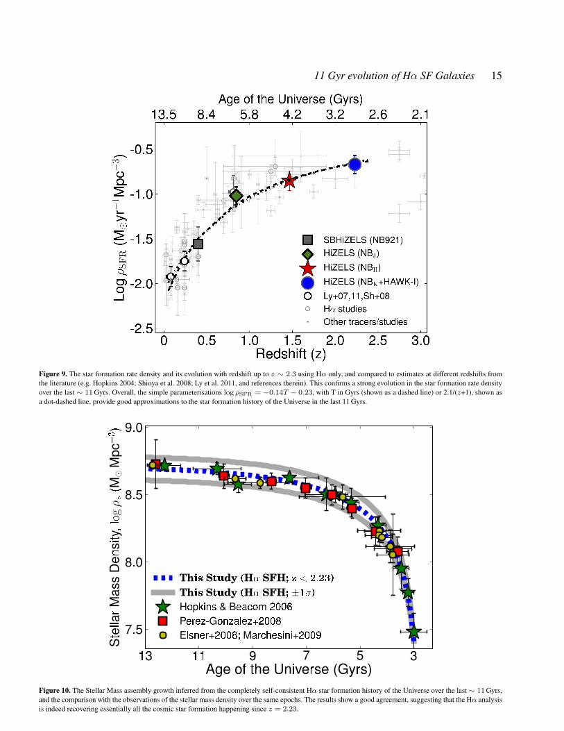
Figure 9. The star formation rate density and its evolution with redshift up to z ∼ 2.3 using Hα only, and compared to estimates at different redshifts fromthe literature (e.g. Hopkins 2004; Shioya et al. 2008; Ly et al. 2011, and references therein). This confirms a strong evolution in the star formation rate densityover the last ∼ 11 Gyrs. Overall, the simple parameterisations log ρSFR = −0.14T − 0.23, with T in Gyrs (shown as a dashed line) or 2.1/(z+1), shown asa dot-dashed line, provide good approximations to the star formation history of the Universe in the last 11 Gyrs.

Figure 10. The Stellar Mass assembly growth inferred from the completely self-consistent Hα star formation history of the Universe over the last ∼ 11 Gyrs,and the comparison with the observations of the stellar mass density over the same epochs. The results show a good agreement, suggesting that the Hα analysisis indeed recovering essentially all the cosmic star formation happening since z = 2.23.

c© 2012 RAS, MNRAS 000, 1–18

16 D. Sobral et al.

at each redshift is recycled, and can be used in subsequent star for-mation episodes. The fraction of recycled mass depends on the IMFused. For a Salpeter IMF, which has been used for the Hα calibra-tion, the recycling fraction is 30%. Note, however, that changingthe IMF does not change the qualitative results presented in thispaper, in particular the agreement between the predicted and themeasured stellar mass density growth. Nevertheless, changing theIMF changes both the normalisation of the star formation historyand the stellar mass density growth.

Here, the following approach is taken: the measured stellarmass density already in place at z ∼ 2.2 (many determinationsexist, e.g. Hopkins & Beacom 2006; Perez-Gonzalez et al. 2008;Ilbert et al. 2009) is assumed to be log10 M = 7.45 MMpc−3.By using the measured Hα star formation history derived in thispaper (log ρSFR = −0.14T − 0.23), a prediction of the evolutionof the stellar mass density of the Universe is computed, using therecycling fraction of the Salpeter IMF (30%).

The results are presented in Figure 10, and compared with var-ious measurements of the stellar mass density at different redshiftsavailable from the literature (Hopkins & Beacom 2006; Perez-Gonzalez et al. 2008; Elsner et al. 2008; Marchesini et al. 2009). Allliterature results have been converted to a Salpeter IMF if derivedwith a different IMF – including those with a modified SalpeterIMF (SalA; resulting in masses a factor of 0.77 lower than Salpeter;see e.g. Hopkins & Beacom).

The results reveal a very good agreement between the predic-tions based on the Hα star formation history of the Universe pre-sented in this paper since z = 2.23 and the stellar mass densityevolution of the Universe, measured directly by many authors. Theresults therefore indicate that at least since z = 2.23 the Hα starformation history of the Universe is a very good representation ofthe total star formation history of the Universe. It is possible to rec-oncile the observed evolution of the stellar mass density with thatproduced from the observed star formation history with very simpleassumptions, without the need to modify the IMF or have it evolveas a function of time. The Hα analysis reveals that star formationsince z = 2.23 is responsible for 95% of the total stellar mass den-sity observed today, with about half of that being assembled fromz ∼ 2.2 to z ∼ 1.2, and the other half since z ≈ 1.2. Note thatthe same conclusion is reached if the stellar mass density at z = 0is adopted for the normalisation (instead of that at z = 2.23), andthe measured Hα star formation history is used (with appropriaterecycling factor) to evolve this stellar mass density back to earlierepochs. Moreover, if the star formation rate density continues todecline with time in the same way as in the last∼ 11 Gyrs, the stel-lar mass density growth will become increasingly slower, with thestellar mass density of the Universe reaching a maximum which isonly 5% higher than currently.

5 CONCLUSIONS

This paper presents new results from a unique combination of wideand deep narrow-band Hα surveys using UKIRT, Subaru and theVLT. It has resulted in robust and equally selected samples of sev-eral hundreds of Hα emitters in narrow redshift slices, allowingto study and parameterise in a completely self-consistent way theevolution of the Hα luminosity function over the last 11 Gyrs ofthe Universe. The main results are:

• We robustly select a total of 1742, 637, 515 and 556 Hα emit-ters (Σ>3, EW0(Hα)>25 A) across the COSMOS and the UDSfields at z = 0.40, 0.84, 1.47 and 2.23, respectively. These are

by far the largest samples of homogeneously selected Hα emitters,while the wide area and the coverage over two independent fieldsallows to greatly overcome cosmic variance and also assemble largesamples of more luminous galaxies.• We find that the Hα luminosity function evolves significantly

from z ∼ 0 to z ∼ 2.2, with the bulk of the evolution being drivenby the continuous rise in L∗Hα by a factor of 10 from the localUniverse to z ∼ 2.2, which is well described by log L∗Hα(z) =0.45z + 41.87

• By obtaining very deep data over a wide range of epochs, it isfound that the faint-end slope, α does not evolve with redshift up toz ∼ 2.3, and is set to α = −1.60± 0.08 for the last 11 Gyrs (0 <z < 2.2), contrarily to previous claims (based on heterogeneoussamples) which argued for a steepening with redshift.• The evolution seen in the Hα luminosity function is in good

agreement with the evolution seen using inhomogeneous compila-tions of other tracers of star formation, such as FIR and UV, jointlypointing towards the bulk of the evolution in the last 11 Gyrs beingdriven by a similar star-forming population across cosmic time, butwith a strong luminosity increase from z ∼ 0 to z ∼ 2.2.• This is the first time Hα has been used to trace SF activity

with a single homogeneous survey at z = 0.4 − 2.23. The simpleparametrisations log ρSFR = −0.14T−0.23 (with T being the ageof the Universe in Gyrs) or log ρSFR = −2.1

(z+1)are good approxi-

mations for the last 11 Gyrs, showing that ρSFR has been decliningsince z ∼ 2.2.• The results reveal that both the shape and normalisation of the

Hα star formation history are consistent with the measurements ofthe stellar mass density growth, confirming that the Hα cosmic starformation history is tracing the bulk of the formation of stars in theUniverse for z < 2.3.• The star formation activity over the last≈ 11 Gyrs is responsi-

ble for producing ∼ 95% of the total stellar mass density observedlocally today, with about half of that being assembled from z ∼ 2.2to z ∼ 1.2, and the other half at z < 1.2.

The results presented in this paper provide a self-consistentview that improves our understanding of the evolution of star-forming galaxies. Particularly, it shows that the evolution of thestar-forming population in the last 11 Gyrs has been mostly drivenby a change in the typical star formation rate of the population(L∗Hα), while the faint-end slope of the Hα LF has remained con-stant, and the change in the normalisation has been much moremoderate. The strong evolution in L∗Hα (or SFR∗) may well beunveiling something very fundamental about the evolution of star-forming galaxies, as it seems to mark a transition between diskand mergers (e.g. S09) in the last 9-10 Gyrs. Also, scaling SFRsby the SFR∗ at each epoch (or Hα luminosities by L∗Hα at eachepoch) seems to recover relatively non-evolving relations betweenscaling SFRs/luminosities and e.g. dust extinction (S12), morpho-logical class (S09), or the typical dark matter halo in which thestar-forming galaxies are likely to reside (Sobral et al. 2010).

The results presented in this paper also complement the cur-rent view on the evolution of the stellar mass function over thelast 11 Gyrs (e.g. Ilbert et al. 2009; Peng et al. 2010; March-esini et al. 2012), which also reveal a non-evolving faint-end slope(of the stellar mass function) at least for z < 2, but shallower,α = −1.3. However, the typical mass of the stellar mass func-tion, M∗, is found to be roughly constant in the last 11 Gyrs, withthe main change being φ∗, which continuously increases in the last∼ 11 Gyrs. Combining the results of the evolution of the Hα lumi-nosity function with those of the evolution of the stellar mass func-

c© 2012 RAS, MNRAS 000, 1–18


tion point towards a star-forming population mostly evolving withan overall decrease in their SFRs/luminosity, and with the over-all population presenting a typical non-evolving mass and simplyevolving by a change in number density, consistent with the sce-nario proposed by Peng et al. (2010).

ACKNOWLEDGMENTS

DS is supported by a NOVA fellowship. IRS acknowledges a Lev-erhulme Senior Fellowship. PNB acknowledges support from theLeverhulme Trust. YM, JPS and IRS thank the U.K. Science andTechnology Facility Council (STFC). JEG is supported by a Bant-ing Fellowship, administered by the Natural Science and Engineer-ing Research Council of Canada. We would like to thank RichardEllis, Simon Lilly, Peter Capak, Adam Muzzin, Taddy Kodama,Masao Hayashi, Andy Lawrence, Joop Schaye, Marijn Franx, HuubRottgering, Rychard Bouwens and Renske Smit for many interest-ing and helpful discussions. We would also like to thank Chun Lyfor helpful comments. The authors wish to thank all the JAC stafffor their help conducting the observations at the UKIRT telescope,and their continuous support and we are also extremely gratefulto all the Subaru staff. We also acknowledge ESO and Subarufor service observations. Finally, the authors fully acknowledgethe tremendous work that has been done by both COSMOS andUKIDSS UDS/SXDF teams in assembling such large, state-of-the-art multi-wavelength data-sets over such wide areas, as those havebeen crucial for the results presented in this paper.

REFERENCES

Arnouts S., Schiminovich D., Ilbert O., Tresse L., Milliard B.,Treyer M., Bardelli S., et al. 2005, ApJL, 619, L43

Atek H., Malkan M., McCarthy P., Teplitz H. I., Scarlata C., SianaB., Henry A., et al. 2010, ApJ, 723, 104

Bertin E., Arnouts S., 1996, A&AS, 117, 393Best P., Smail I., Sobral D., Geach J., Garn T., Ivison R., Kurk J.,

Dalton G., Cirasuolo M., Casali M., 2010, arXiv:1003.5183Bunker A. J., Warren S. J., Hewett P. C., Clements D. L., 1995,

MNRAS, 273, 513Casali M., Pirard J.-F., Kissler-Patig M., Moorwood A., Bedin L.,

Biereichel P., Delabre B., et al. 2006, in Society of Photo-OpticalInstrumentation Engineers (SPIE) Conference Series Vol. 6269of Society of Photo-Optical Instrumentation Engineers (SPIE)Conference Series, HAWK-I: the new wide-field IR imager forthe VLT

Cirasuolo M., McLure R. J., Dunlop J. S., Almaini O., FoucaudS., Simpson C., 2010, MNRAS, 401, 1166

Cutri R. M., Skrutskie M. F., van Dyk S., Beichman C. A., Car-penter J. M., Chester T., Cambresy L., et al. 2003, 2MASS AllSky Catalog of point sources.

Daddi E., Cimatti A., Renzini A., Fontana A., Mignoli M.,Pozzetti L., Tozzi P., Zamorani G., 2004, ApJ, 617, 746

Dutton A. A., van den Bosch F. C., Dekel A., 2010, MNRAS, 405,1690

Elsner F., Feulner G., Hopp U., 2008, A&A, 477, 503Gallego J., Zamorano J., Aragon-Salamanca A., Rego M., 1995,

ApJL, 455, L1Garn T., Sobral D., Best P. N., Geach J. E., Smail I., Cirasuolo

M., Dalton G. B., Dunlop J. S., McLure R. J., Farrah D., 2010,MNRAS, 402, 2017

Geach J. E., Simpson C., Rawlings S., Read A. M., Watson M.,2008, VizieR Online Data Catalog, 838, 11369

Geach J. E., Smail I., Best P. N., Kurk J., Casali M., Ivison R. J.,Coppin K., 2008, MNRAS, 388, 1473

Gilbank D. G., Baldry I. K., Balogh M. L., Glazebrook K., BowerR. G., 2010, MNRAS, 405, 2594

Glazebrook K., Abraham R. G., McCarthy P. J., Savaglio S., ChenH.-W., Crampton D., Murowinski R., et al. 2004, Nature, 430,181

Gonzalez V., Labbe I., Bouwens R. J., Illingworth G., Franx M.,Kriek M., Brammer G. B., 2010, ApJ, 713, 115

Hayes M., Schaerer D., Ostlin G., 2010, A&A, 509, L5+Hopkins A. M., 2004, ApJ, 615, 209Hopkins A. M., Beacom J. F., 2006, ApJ, 651, 142Hopkins A. M., Connolly A. J., Haarsma D. B., Cram L. E., 2001,

AJ, 122, 288Hopkins A. M., Connolly A. J., Szalay A. S., 2000, AJ, 120, 2843Ilbert O., Capak P., Salvato M., Aussel H., McCracken H. J.,

Sanders D. B., Scoville N., et al. 2009, ApJ, 690, 1236Lawrence A., Warren S. J., Almaini O., Edge A. C., Hambly N. C.,

Jameson R. F., Lucas P., et al. 2007, MNRAS, 379, 1599Lilly S. J., Le Brun V., Maier C., Mainieri V., Mignoli M., Scodeg-

gio M., Zamorani G., et al. 2009, ApJS, 184, 218Lilly S. J., Le Fevre O., Hammer F., Crampton D., 1996, ApJL,

460, L1Ly C., Lee J. C., Dale D. A., Momcheva I., Salim S., Staudaher

S., Moore C. A., Finn R., 2011, ApJ, 726, 109Ly C., Malkan M. A., Kashikawa N., Shimasaku K., Doi M., Na-

gao T., Iye M., et al. 2007, ApJ, 657, 738Malkan M., Teplitz H., McLean I., 1995, ApJL, 448, L5Marchesini D., Stefanon M., Brammer G. B., Whitaker K. E.,

2012, arXiv:1201.6365Marchesini D., van Dokkum P. G., Forster Schreiber N. M., Franx

M., Labbe I., Wuyts S., 2009, ApJ, 701, 1765McCarthy P. J., Yan L., Freudling W., Teplitz H. I., Malumuth

E. M., Weymann R. J., Malkan M. A., et al. 1999, ApJ, 520, 548Moorwood A. F. M., van der Werf P. P., Cuby J. G., Oliva E., 2000,

A&A, 362, 9Oesch P. A., Bouwens R. J., Carollo C. M., Illingworth G. D.,

Magee D., Trenti M., Stiavelli M., Franx M., Labbe I., vanDokkum P. G., 2010, ApJL, 725, L150

Ono Y., Ouchi M., Shimasaku K., Akiyama M., Dunlop J., FarrahD., et al.. 2010, MNRAS, 402, 1580

Ouchi M., Shimasaku K., Akiyama M., Simpson C., Saito T.,Ueda Y., Furusawa H., et al. 2008, ApJS, 176, 301

Ouchi M., Shimasaku K., Furusawa H., Saito T., Yoshida M.,Akiyama M., Ono Y., et al. 2010, ApJ, 723, 869

Ouchi M., Shimasaku K., Okamura S., Furusawa H., KashikawaN., Ota K., Doi M., et al. 2004, ApJ, 611, 660

Peng Y.-j., Lilly S. J., Kovac K., Bolzonella M., Pozzetti L., Ren-zini A., Zamorani G., et al. 2010, ApJ, 721, 193

Perez-Gonzalez P. G., Rieke G. H., Villar V., Barro G., BlaylockM., Egami E., Gallego J., et al. 2008, ApJ, 675, 234

Pirard J.-F., Kissler-Patig M., Moorwood A., Biereichel P., De-labre B., Dorn R., Finger G., et al. 2004, in A. F. M. Moor-wood & M. Iye ed., Society of Photo-Optical InstrumentationEngineers (SPIE) Conference Series Vol. 5492 of Society ofPhoto-Optical Instrumentation Engineers (SPIE) Conference Se-ries, HAWK-I: A new wide-field 1- to 2.5-µm imager for theVLT. pp 1763–1772

Salim S., Rich R. M., Charlot S., Brinchmann J., Johnson B. D.,Schiminovich D., Seibert M., et al. 2007, ApJS, 173, 267

c© 2012 RAS, MNRAS 000, 1–18

18 D. Sobral et al.

Scoville N., Aussel H., Brusa M., Capak P., Carollo C. M., ElvisM., Giavalisco M., et al 2007, ApJS, 172, 1

Shim H., Chary R.-R., Dickinson M., Lin L., Spinrad H., SternD., Yan C.-H., 2011, arXiv:1103.4124

Shioya Y., Taniguchi Y., Sasaki S. S., Nagao T., Murayama T.,Takahashi M. I., Ajiki M., et al. 2008, ApJS, 175, 128

Simpson C., Martınez-Sansigre A., Rawlings S., Ivison R.,Akiyama M., Sekiguchi K., Takata T., Ueda Y., Watson M.,2006, MNRAS, 372, 741

Smail I., Sharp R., Swinbank A. M., Akiyama M., Ueda Y., Fou-caud S., Almaini O., Croom S., 2008, MNRAS, 389, 407

Sobral D., Best P., Matsuda Y., Smail I., Geach J., Cirasuolo M.,2012, arXiv:1109.1830

Sobral D., Best P. N., Geach J. E., Smail I., Cirasuolo M., GarnT., Dalton G. B., Kurk J., 2010, MNRAS, 404, 1551

Sobral D., Best P. N., Geach J. E., Smail I., Kurk J., Cirasuolo M.,Casali M., et al. 2009, MNRAS, 398, 75

Sobral D., Best P. N., Smail I., Geach J. E., Cirasuolo M., GarnT., Dalton G. B., 2011, MNRAS, 411, 675

Straughn A. N., Kuntschner H., Kummel M., Walsh J. R., CohenS. H., Gardner J. P., Windhorst R. A., et al. 2011, AJ, 141, 14

Tadaki K.-I., Kodama T., Koyama Y., Hayashi M., Tanaka I.,Tokoku C., 2011, PASJ, 63, 437

Treyer M. A., Ellis R. S., Milliard B., Donas J., Bridges T. J.,1998, MNRAS, 300, 303

van Breukelen C., Cotter G., Rawlings S., Readhead T., BonfieldD., Clewley L., Ivison R., Jarvis M., Simpson C., Watson M.,2007, MNRAS, 382, 971

van Dokkum P. G., Brammer G., Fumagalli M., Nelson E., FranxM., Rix H.-W., Kriek M., Patel S., et al. 2011, ApJL, 743, L15

Villar V., Gallego J., Perez-Gonzalez P. G., Pascual S., Noeske K.,Koo D. C., Barro G., Zamorano J., 2008, ApJ, 677, 169

Yagi M., Kashikawa N., Sekiguchi M., Doi M., Yasuda N., Shi-masaku K., Okamura S., 2002, AJ, 123, 66

Yamada T., Kodama T., Akiyama M., Furusawa H., Iwata I., Ka-jisawa M., Iye M., Ouchi M., et al. 2005, ApJ, 634, 861

Yan L., McCarthy P. J., Freudling W., Teplitz H. I., MalumuthE. M., Weymann R. J., Malkan M. A., 1999, ApJL, 519, L47

APPENDIX A: CATALOGUES OF CANDIDATE HIZELSNARROW-BAND EMITTERS

The catalogues of potential narrow-band emitters over the COS-MOS and UDS fields are presented in Tables A.1 (NB921), A.2(NBJ), A.3 (NBH) and A.4 (NBK). It contains IDs (includingfield and observing band), Right Ascension (RA), Declination(Dec), narrow-band magnitude (NB), broad-band magnitude (BB),the significance of the narrow-band excess (Σ), Estimated Flux(log 10), estimated observed EW, and a flag for those that are clas-sified as Hα. Note that only the online version contains the full cat-alogue – here only five entries of the table are shown as examplesof the entire catalogues.

This paper has been typeset from a TEX/ LATEX file prepared by theauthor.

c© 2012 RAS, MNRAS 000, 1–18


Table A1. A catalogue of all Σ > 3 NB921 narrow-band sources selected in the UDS and COSMOS fields from HiZELS. NB magnitudes are NB921 (AB);BB are z′ magnitudes (AB). Note that on the printed version this only contains 5 entries, in order to provide some examples contained in the full catalogue.The full catalogue is available on-line.

ID R.A. Dec. NB BB Σ log Flux EWobs Hα selected(J2000) (J2000) (AB) (AB) erg s−1 A

HiZELS-COSMOS-NB921-S12-14 09 58 13.57 +02 17 15.6 23.86±0.11 24.85±0.08 13.6 −16.255 418.4 NoHiZELS-COSMOS-NB921-S12-105 09 59 57.96 +02 17 41.5 23.14±0.03 23.39±0.02 9.9 −16.132 119.8 NoHiZELS-COSMOS-NB921-S12-136 09 58 57.55 +02 17 45.0 21.64±0.01 22.11±0.01 56.5 −15.636 105.9 YesHiZELS-COSMOS-NB921-S12-4064 09 59 20.49 +02 20 54.5 22.06±0.01 22.21±0.01 14.3 −16.084 39.13 No

HiZELS-UDS-NB921-S12-220582 02 16 19.37 −05 13 54.2 22.37±0.01 22.65±0.01 55.6 −16.287 38.22 Yes

Table A2. A catalogue of all Σ > 3 NBJ narrow-band sources selected in the UDS and COSMOS fields from HiZELS. NB magnitudes are NBJ (Vega);BB are J magnitudes (Vega). Note that on the printed version this only contains 5 example entries, in order to provide some examples contained in the fullcatalogue. The full catalogue is available on-line.

ID R.A. Dec. NB BB Σ log Flux EWobs Hα selected(J2000) (J2000) (Vega) (Vega) erg s−1 A

HiZELS-COSMOS-NBJ-S12-206 09 58 42.11 +01 58 40.5 21.58±0.20 22.83±0.23 3.5 −16.11 463.5 NoHiZELS-COSMOS-NBJ-S12-292 09 58 42.65 +02 27 24.2 20.51±0.08 20.85±0.05 3.7 −16.08 65.4 YesHiZELS-COSMOS-NBJ-S12-293 09 58 42.63 +02 19 53.2 20.84±0.10 21.46±0.07 4.4 −16.01 139.3 Yes

HiZELS-UDS-NBJ-S12-5 02 16 16.81 −05 09 09.2 20.51±0.08 20.85±0.05 5.4 −15.89 194.6 YesHiZELS-UDS-NBJ-S12-26 02 16 17.15 −05 07 42.4 20.84±0.10 21.46±0.07 4.6 −15.96 79.8 Yes

Table A3. A catalogue of all Σ > 3 NBH narrow-band sources selected in the UDS and COSMOS fields from HiZELS. NB magnitudes are NBH (Vega);BB are H magnitudes (Vega). Note that on the printed version this only contains 5 example entries, in order to provide some examples contained in the fullcatalogue. The full catalogue is available on-line.


HiZELS-COSMOS-NBH-S12-206 09 57 47.31 +02 02 08.1 21.58±0.14 20.99±0.05 3.1 −15.98 251.4 NoHiZELS-COSMOS-NBH-S12-292 09 57 47.33 +01 51 53.1 20.51±0.02 18.33±0.01 12.1 −15.40 77.3 NoHiZELS-COSMOS-NBH-S12-293 09 57 47.65 +02 16 19.8 20.84±0.08 19.80±0.02 3.3 −15.87 101.8 No

HiZELS-UDS-NBH-S12-4012 02 16 44.17 −04 44 53.0 20.04±0.18 20.93±0.04 3.0 −15.87 308 YesHiZELS-UDS-NBH-S12-4136 02 16 45.35 −04 07 26.8 19.15±0.08 19.76±0.02 5.2 −15.64 171 Yes

Table A4. A catalogue of all Σ > 3 NBK narrow-band sources selected in the UDS and COSMOS fields from HiZELS. NB magnitudes are NBK (Vega);BB are K magnitudes (Vega). Note that on the printed version this only contains 5 example entries, in order to provide some examples contained in the fullcatalogue. The full catalogue is available on-line.


HiZELS-COSMOS-NBK-S12-2227 09 58 14.05 +02 34 05.1 20.26±0.23 21.68±0.16 3.1 −16.31 728 YesHiZELS-COSMOS-NBK-S12-45390 10 00 59.58 +02 44 35.9 19.24±0.09 19.92±0.04 5.4 −16.09 208 NoHiZELS-COSMOS-NBKS12-44193 10 00 55.39 +01 59 55.1 19.02±0.06 19.68±0.02 7.6 −16.01 198 Yes

HiZELS-UDS-NBK-S12-15961 02 18 09.03 −04 47 49.9 17.47±0.02 18.27±0.01 30.6 −15.33 262 YesHiZELS-UDS-NBK-S12-22618 02 18 53.02 −05 01 07.7 19.36±0.10 20.02±0.02 4.5 −16.16 196 No

c© 2012 RAS, MNRAS 000, 1–18

A large H survey at z = 2.23, 1.47, 0.84 and 0.40: the 11 Gyr evolution of star-forming galaxies...

Documents

Transcript of A large H survey at z = 2.23, 1.47, 0.84 and 0.40: the 11 Gyr evolution of star-forming galaxies...