A geometric characterisation of the quadratic

min-power centre

M. Brazil, C.J. Ras, D.A. Thomas

Abstract

For a given set of nodes in the plane the min-power centre is a point such

that the cost of the star centred at this point and spanning all nodes is min-

imised. The cost of the star is defined as the sum of the costs of its nodes, where

the cost of a node is an increasing function of the length of its longest incident

edge. The min-power centre problem provides a model for optimally locating

a cluster-head amongst a set of radio transmitters, however, the problem can

also be formulated within a bicriteria location model involving the 1-centre

and a generalized Fermat-Weber point, making it suitable for a variety of facil-

ity location problems. We use farthest point Voronoi diagrams and Delaunay

triangulations to provide a complete geometric description of the min-power

centre of a finite set of nodes in the Euclidean plane when cost is a quadratic

function. This leads to a new linear-time algorithm for its construction when

the convex hull of the nodes is given. We also provide an upper bound for the

performance of the centroid as an approximation to the quadratic min-power

centre. Finally, we briefly describe the relationship between solutions under

quadratic cost and solutions under more general cost functions.

Keywords: networks, power efficient range assignment, wireless ad hoc net-

works, generalised Fermat-Weber problem, farthest point Voronoi diagrams

1 Introduction

One of the most important problems in the optimal design of wireless ad hoc radio

networks is that of power minimisation. This is true during the physical design phase

1

arX

iv:1

307.

1222

v1 [

mat

h.O

C]

4 J

ul 2

013

and when designing efficient routing protocols [16, 22, 23]. The most appropriate

fundamental model in both cases is the power efficient range assignment problem,

where communication ranges are assigned to all transmitters such that total power

is minimised. It is assumed that the power of each transmitter is proportional to its

assigned communication range raised to an exponent α > 1 (see [1]). The process of

assigning communication ranges therefore determines the total power output as well

as the available communication topology of the resultant network.

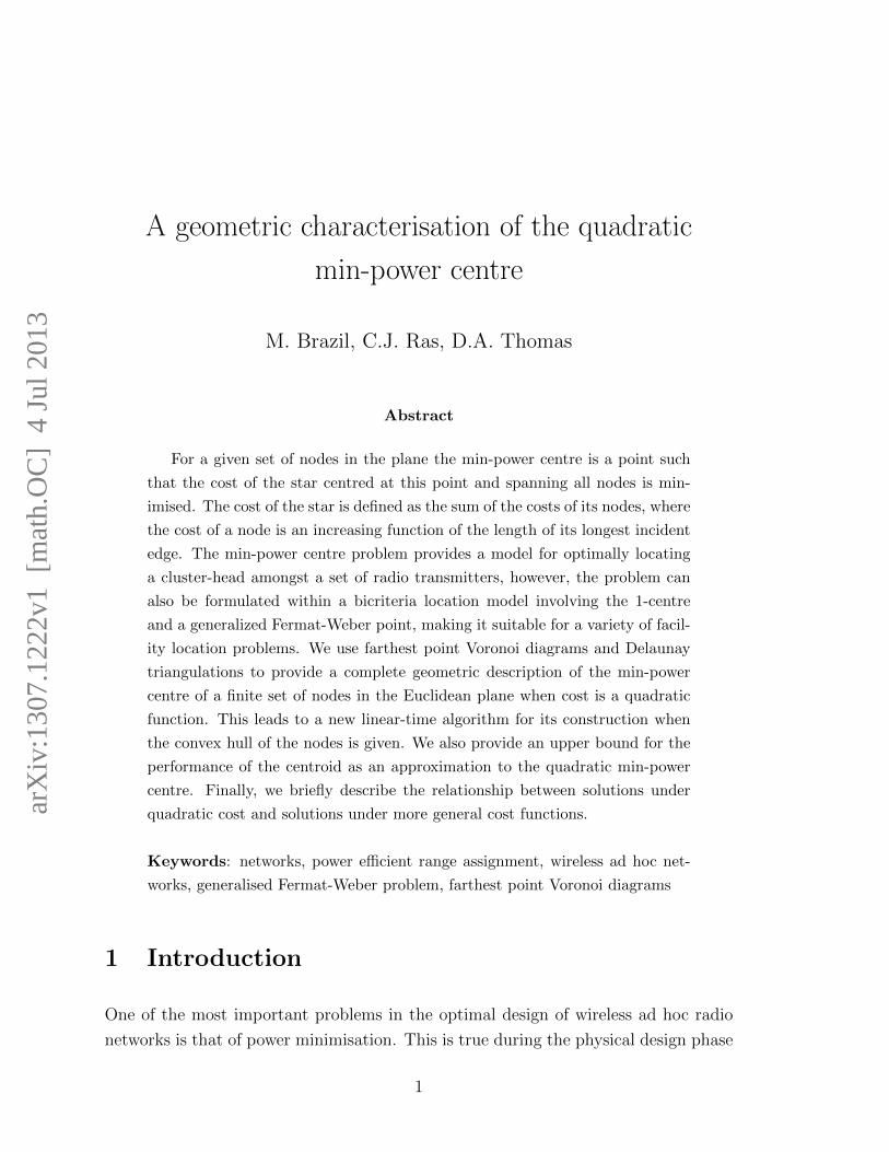
The range assignment problem is a type of disk covering problem, where the centres

of the disks are given nodes, the radii (ri) of the disks are transmission ranges, and the

directed graph induced by the disks (see Figure 1, where bidirected edges are depicted

without arrows) must satisfy a given connectivity constraint whilst minimising∑rαi .

The exponent α is called the path loss exponent and most commonly takes a value

between 2 and 4, with α = 2 corresponding to transmission in free-space. For any

α > 1 the range assignment problem is NP-hard, even in the case when only 1-

connectivity is required of the resultant network [13].

(a) (b)

Figure 1: Examples of range assignment-induced graphs

During the design or maintenance of ad hoc radio networks it is often pertinent

to introduce relays or cluster-heads for the processing of aggregated data and for

the improved routing efficiency that takes place in such hierarchical structures (see

[7, 18, 20]). Solving the range assignment problem whilst allowing for the introduction

of a bounded number of additional nodes anywhere in the plane constitutes a very

general and highly applicable geometric network problem, which has only been solved

2

in certain restricted settings (see for instance [3, 4]). Since the optimal locations of

the cluster-heads must be found, as well as the optimal assignment of ranges on the

complete set of nodes, this so called geometric range assignment problem is at least

as difficult as the classical range assignment problem.

This paper considers the problem of optimally locating a single cluster-head amongst

a given set of transmitters, where each transmitter can send and receive data directly

from the cluster-head. Not only is this an interesting and applicable model in it

own right, but it is also a necessary first step in understanding the local structure of

optimal networks with multiple cluster-heads. The graph induced by the assignment

of ranges, in this case, contains an undirected star with the cluster head as its centre

and the complete set of transmitters as its leaves; see for instance Figure 1(b), where

edges between transmitters are depicted as broken lines since they do not contribute

to the cost (power) of the star.

In more formal terms we denote the given finite set of transmitters by X ⊂ R2 and

the cluster-head by s ∈ R2. The power of any x ∈ X is Px = ‖s− x‖α and the power

of s is Ps = max{‖s − x‖α : x ∈ X}, where ‖ · ‖ is the Euclidean norm. The total

power of the system is denoted by P (s) = Ps +∑x∈X

Px, and a min-power centre of X

is a point s∗ which minimises P (s). Minimising only Ps is clearly equivalent to the 1-

centre problem, i.e., the problem of finding the centre of a minimum spanning circle for

X. Minimising only∑Px is a generalised Fermat-Weber problem [5], which becomes

the classical Fermat-Weber problem when α = 1 and the problem of constructing the

centroid when α = 2.

A related concept in facility location is the computation of the center-median (or

cent-dian) of a finite set of points [6], which also has applications in wireless ad

hoc networks for finding a so called core node [9]. In this problem the task is to

find all Pareto-optimal solutions to the vector function Φ(s) = (Ps,∑Px), which is

equivalent to finding the optimal value of λPs + (1 − λ)∑Px for every λ ∈ [0, 1]

(see [8, 12]). Clearly the min-power centre will be optimal for this problem when

λ = 1/2. The vector minimisation problem has also been considered for α = 1 in

the rectilinear plane [15] and for α = 2 in the Euclidean plane [17]. These types of

bicriteria models have been described as seeking a balance between the antagonistic

objectives of efficiency (i.e., the minisum component) and equity (i.e., the minimax

component).

3

There are numerical methods, for instance the sub-gradient method, that optimally

locate s∗ to within any finite precision. However, structural results for the min-

power centre problem, of the type described in this paper, are necessary for optimally

constructing more complex geometric range assignment networks (which is the over-

arching goal of our research). This fact is particularly manifest in the design of

algorithmic pruning modules, where one develops strategies based on properties of

locally optimal structures for eliminating suboptimal network topologies from the ex-

ponential set of possible topologies. The ultimate benefits of good pruning modules

has been demonstrated a number of times for problems similar to the geometric range

assignment problem [3, 4, 21].

In this paper we mostly focus on the quadratic case, α = 2. In terms of cluster-head

placement this means that radio transmission takes place in free space, that is, in an

ideal medium with zero resistance. Path loss exponents close to 2 frequently occur in

real-world wireless radio network scenarios. This is true for transmission in mediums

of low resistance, and in mediums of higher resistance when there is a degree of beam

forming (constructive interference) [14]. The quadratic case also applies to certain

classical facility location problems, including the location of emergency facilities such

as hospitals and fire stations [12, 17, 19]. Furthermore, as demonstrated in the final

section, it is anticipated that theoretical developments in the α = 2 case will lead to

solutions and approximations for other α > 1.

In Section 2 we provide definitions and set up a Karush-Kuhn-Tucker formulation of

the min-power centre problem and its dual for any α > 1. When α = 2 the geometric

construction of the min-power centre becomes tractable, allowing us to provide a

characterisation of the solution in terms of the farthest point Voronoi diagram on

X, and its dual, the farthest point Delaunay triangulation. This characterisation

is described in Section 3, where we also present a new linear-time algorithm for the

construction of the optimal quadratic min-power centre. For α = 2, Section 4 explores

the significance of the centroid and the 1-centre of a set of points for the min-power

centre problem, and provides a characterisation of point sets for which the min-power

centre and the 1-centre coincide. Section 4 also provides a bound for the performance

of the centroid as an approximation to the min-power centre. The final section briefly

explores the general α > 1 case.

4

2 Definitions and analytical properties

Let X = {xi : i ∈ J} be a given finite set of points in the Euclidean plane with index-

set J , and let α > 1 be a given real number. For any point s ∈ R2 let G = G(s,X)

be the undirected star with centre s and leaf-set X. The power of G with respect to

s is denoted by

P (s) = Pα(s,X) =∑i∈J

‖s− xi‖α + maxi∈J{‖s− xi‖α},

where ‖ · ‖ is the Euclidean norm. The first terms of of P (s) can be thought of as

representing the total power required by the existing transmitters for communicating

with the cluster-head, while the second term can be thought of as the power required

by the cluster-head for communicating with the transmitters.

Definition: The Euclidean min-power centre problem on X is the problem of finding

a point s∗α ∈ arg mins

P (s). We refer to s∗ = s∗α as a min-power centre of X.

Lemma 1 For any X the function P (s) is strictly convex, and therefore s∗ is unique.

Proof. This follows since ‖s− xi‖α is strictly convex when α > 1.

Although P (s) is not smooth, it can be expressed as the maximum of a set of smooth

functions: for any j ∈ J let Fj(s) = Fαj (s,X) = ‖s − xj‖α +

∑i∈J

‖s − xi‖α. Then

P (s) = maxj∈J{Fj(s)}. Since α > 1, the gradient

∇(‖s− xi‖α) =

{α(s− xi)‖s− xi‖α−2 : s 6= xi,

0 : s = xi,

is continuous. Therefore Fj is continuously differentiable and convex, since it is the

sum of such functions.

Next we describe a useful non-linear programming formulation of the problem of

finding s∗. Consider the following non-linear optimization program.

5

Problem P1.

minimise(s,v)∈R2×R

v

subject to

Fj(s)− v ≤ 0, ∀j ∈ J.

Clearly Problem P1 is smooth and convex. It is easy to see that (s, v) is optimal for

this problem if and only if s = s∗ and v = P (s∗).

Lemma 2 Problem P1 satisfies the Mangasarian-Fromovitz constraint qualification

for any point (s, v) ∈ R2 × R.

Proof. Note that

〈∇(Fj(s)− v), ((0, 0), 1)〉 = 〈(∇Fj(s),−1), ((0, 0), 1)〉 < 0

for all j such that P (s) = Fj(s).

By the previous lemma and the resulting KKT conditions it follows that the point

(s∗, v∗) ∈ R2 × R is optimal for Problem P1 if and only if there exist multipliers

λ∗j ≥ 0, j ∈ J such that ∇v +∑j∈J

λ∗j(∇Fj(s∗),−1) = 0 and λ∗j(Fj(s∗) − v∗) = 0 for

all j ∈ J . Observe that

λ∗j(Fj(s∗)− v∗) = 0⇔ λ∗j(Fj(s

∗)− P (s∗)) = 0

⇔ λ∗j(‖s∗ − xj‖α −maxi∈J{‖s∗ − xi‖α}) = 0

⇔ λ∗j(‖s∗ − xj‖ −maxi∈J{‖s∗ − xi‖}) = 0

Therefore we can state equivalent KKT conditions as follows: s∗ is the min-power

centre of X if and only if there exists λ∗j ≥ 0 such that

∑j∈J

λ∗j∇Fj(s∗) = 0, (1)∑j∈J

λ∗j = 1, (2)

λ∗j(‖s∗ − xj‖ −maxi∈J{‖s∗ − xi‖}) = 0, ∀j ∈ J. (3)

6

Let n = |J | and let λ = (λ1, ..., λn). The dual of Problem P1 can be written as

Problem D1.

maximiseλ∈Rn

mins∈R2

∑j∈J

(1 + λj)‖s− xj‖α

subject to

λ ≥ 0,∑j∈J

λj = 1.

Finally, we can convert the dual problem to a more familiar form as follows. For

every j ∈ J let τj =λj + 1

n+ 1. Therefore

1

n+ 1≤ τj and

∑j∈J

τj = 1. Let s(τ) =

arg mins∈R2

∑j∈J

τj‖s − xj‖α (observe that s(τ) is unique). Clearly then∑j∈J

τj∇(‖s(τ) −

xj‖α) = 0, which is equivalent to∑j∈J

τj(s(τ) − xj)‖s(τ) − xj‖α−2 = 0. Therefore an

equivalent formulation of Problem D1 is:

Problem D1′.

maximiseτ∈Rn

(n+ 1)∑j∈J

τj‖s− xj‖α (4)

subject to

1

n+ 1≤ τj, (5)∑

j∈J

τj = 1, (6)∑j∈J

τj(s− xj)‖s− xj‖α−2 = 0. (7)

If τ ∗ is optimal for Problem D1′ then s∗ = s(τ ∗) is optimal for Problem P1 and

λ∗ = (n + 1)τ ∗ − 1 gives the multipliers satisfying Equations (1)-(3). This final

formulation is recognisable in that it is almost identical to the dual of the problem

minimises∈R2

maxj∈J||s− xj||α,

7

which is the well-known minimum spanning circle problem (see [10] for a derivation).

The only two differences in these duals are Inequality (5), which will be replaced by

τj ≥ 0 for the minimum spanning circle problem, and the extra coefficient n + 1 of

the objective function. In general, the restriction on domain specified by Inequality 5

leads to a non-trivial variation on the minimum spanning circle problem, however, as

shown in the next section, for α = 2 there exists an interesting and useful geometric

relationship between the minimum spanning circle problem and the min-power centre

problem.

3 The geometry of α = 2

In order to study the geometry of the case where α = 2 we first rewrite the KKT

conditions in terms of the 2-centroids of X.

Definition: Recall that the centroid (or centre of mass) of X, which we denote as

M , is defined by M =1

n

∑j∈J

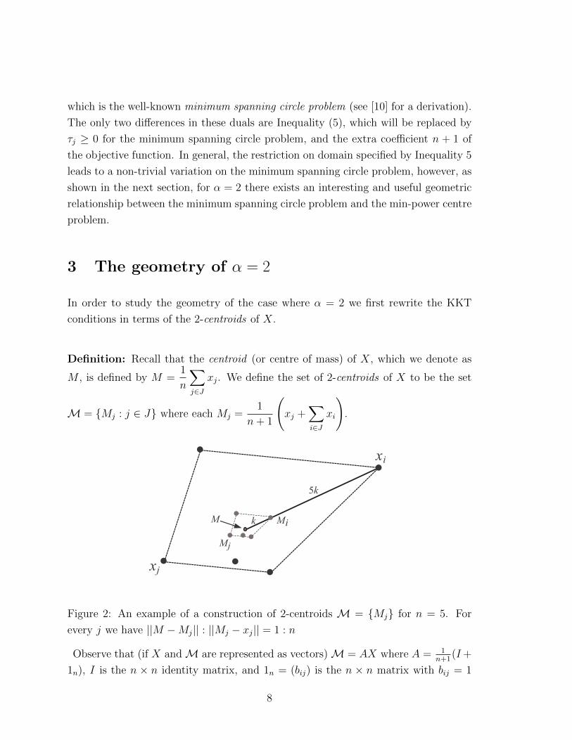
xj. We define the set of 2-centroids of X to be the set

M = {Mj : j ∈ J} where each Mj =1

n+ 1

(xj +

∑i∈J

xi

).

xi

Mi

xj

Mj

M

5k

k

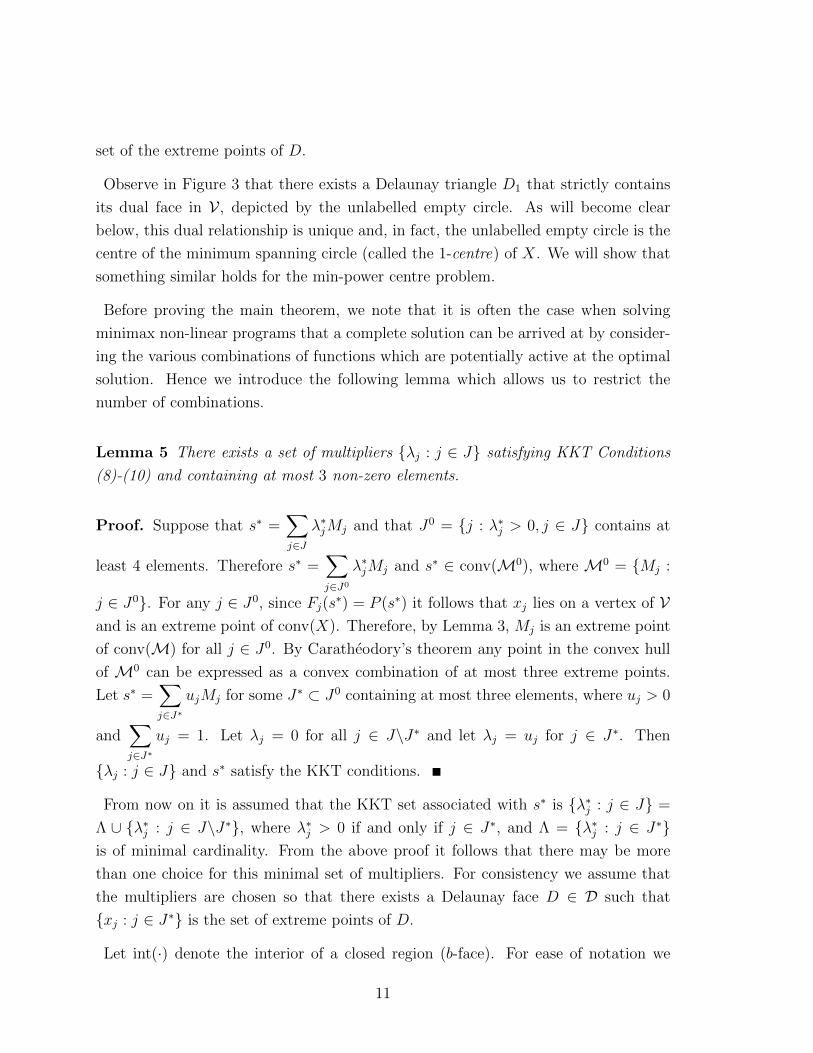
Figure 2: An example of a construction of 2-centroids M = {Mj} for n = 5. For

every j we have ||M −Mj|| : ||Mj − xj|| = 1 : n

Observe that (if X andM are represented as vectors)M = AX where A = 1n+1

(I+

1n), I is the n × n identity matrix, and 1n = (bij) is the n × n matrix with bij = 1

8

for all i, j. This means that M is the image of an affine transformation on X. An

consequence of this observation is the following lemma. Let conv(·) denote the the

convex hull of a set of points.

Lemma 3 The region conv(M) is similar to conv(X), and M is the centroid of M.

For any j the point Mj divides the line segment Mxj into a ratio of 1 : n (see Figure

2, where the Mj are grey-filled circles).

For any X ′ ⊆ conv(X) we denote (with a slight abuse of notation) the image of X ′

under the above affine transformation by AX ′, which is a subset of conv(M). We

also similarly employ A−1 for the inverse transformation.

In the quadratic case (where α = 2) we now write

∇Fj(s) = 2(n+ 1)s− 2xj − 2∑i∈J

xi

= 2(n+ 1)(s−Mj).

This equation implies that for any j we have Mj = arg mins

{‖xj − s‖2 +∑

i∈J ‖xi−

s‖2}. In the case α = 2 a simplified set of KKT conditions for Problem P1 in total is

s∗ =∑j∈J

λ∗jMj, (8)∑j∈J

λ∗j = 1, (9)

λ∗j(‖s∗ − xj‖ −maxi∈J{‖s∗ − xi‖}) = 0, ∀j ∈ J. (10)

By Condition 8 we have:

Lemma 4 s∗ ∈ conv(M).

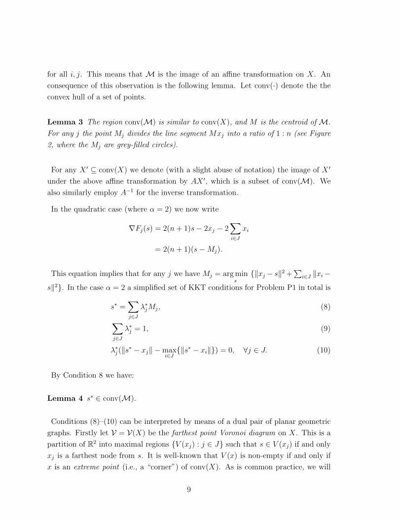
Conditions (8)–(10) can be interpreted by means of a dual pair of planar geometric

graphs. Firstly let V = V(X) be the farthest point Voronoi diagram on X. This is a

partition of R2 into maximal regions {V (xj) : j ∈ J} such that s ∈ V (xj) if and only

xj is a farthest node from s. It is well-known that V (x) is non-empty if and only if

x is an extreme point (i.e., a “corner”) of conv(X). As is common practice, we will

9

(without confusion) treat V both as a graph specified by the boundary edges, or as a

partition of the plane. It is well known that V is a tree.

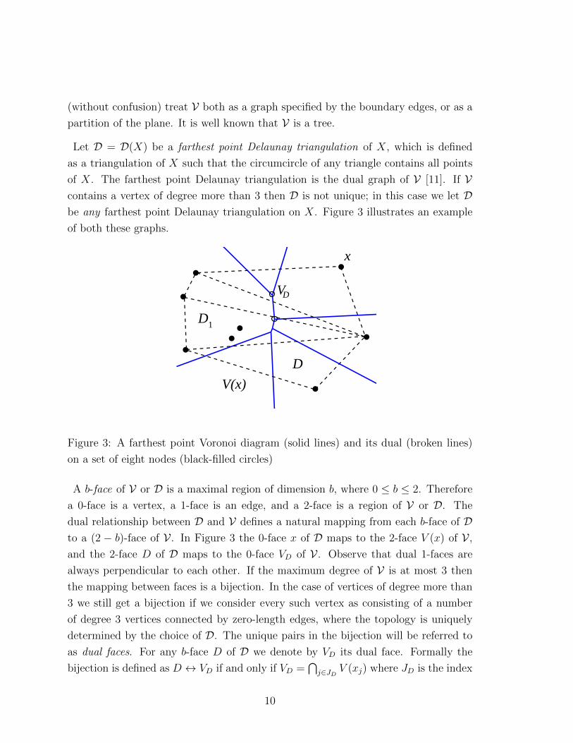
Let D = D(X) be a farthest point Delaunay triangulation of X, which is defined

as a triangulation of X such that the circumcircle of any triangle contains all points

of X. The farthest point Delaunay triangulation is the dual graph of V [11]. If Vcontains a vertex of degree more than 3 then D is not unique; in this case we let Dbe any farthest point Delaunay triangulation on X. Figure 3 illustrates an example

of both these graphs.

D1

D

x

V

V(x)

D

Figure 3: A farthest point Voronoi diagram (solid lines) and its dual (broken lines)

on a set of eight nodes (black-filled circles)

A b-face of V or D is a maximal region of dimension b, where 0 ≤ b ≤ 2. Therefore

a 0-face is a vertex, a 1-face is an edge, and a 2-face is a region of V or D. The

dual relationship between D and V defines a natural mapping from each b-face of Dto a (2 − b)-face of V . In Figure 3 the 0-face x of D maps to the 2-face V (x) of V ,

and the 2-face D of D maps to the 0-face VD of V . Observe that dual 1-faces are

always perpendicular to each other. If the maximum degree of V is at most 3 then

the mapping between faces is a bijection. In the case of vertices of degree more than

3 we still get a bijection if we consider every such vertex as consisting of a number

of degree 3 vertices connected by zero-length edges, where the topology is uniquely

determined by the choice of D. The unique pairs in the bijection will be referred to

as dual faces. For any b-face D of D we denote by VD its dual face. Formally the

bijection is defined as D ↔ VD if and only if VD =⋂j∈JD V (xj) where JD is the index

10

set of the extreme points of D.

Observe in Figure 3 that there exists a Delaunay triangle D1 that strictly contains

its dual face in V , depicted by the unlabelled empty circle. As will become clear

below, this dual relationship is unique and, in fact, the unlabelled empty circle is the

centre of the minimum spanning circle (called the 1-centre) of X. We will show that

something similar holds for the min-power centre problem.

Before proving the main theorem, we note that it is often the case when solving

minimax non-linear programs that a complete solution can be arrived at by consider-

ing the various combinations of functions which are potentially active at the optimal

solution. Hence we introduce the following lemma which allows us to restrict the

number of combinations.

Lemma 5 There exists a set of multipliers {λj : j ∈ J} satisfying KKT Conditions

(8)-(10) and containing at most 3 non-zero elements.

Proof. Suppose that s∗ =∑j∈J

λ∗jMj and that J0 = {j : λ∗j > 0, j ∈ J} contains at

least 4 elements. Therefore s∗ =∑j∈J0

λ∗jMj and s∗ ∈ conv(M0), where M0 = {Mj :

j ∈ J0}. For any j ∈ J0, since Fj(s∗) = P (s∗) it follows that xj lies on a vertex of V

and is an extreme point of conv(X). Therefore, by Lemma 3, Mj is an extreme point

of conv(M) for all j ∈ J0. By Caratheodory’s theorem any point in the convex hull

of M0 can be expressed as a convex combination of at most three extreme points.

Let s∗ =∑j∈J∗

ujMj for some J∗ ⊂ J0 containing at most three elements, where uj > 0

and∑j∈J∗

uj = 1. Let λj = 0 for all j ∈ J\J∗ and let λj = uj for j ∈ J∗. Then

{λj : j ∈ J} and s∗ satisfy the KKT conditions.

From now on it is assumed that the KKT set associated with s∗ is {λ∗j : j ∈ J} =

Λ ∪ {λ∗j : j ∈ J\J∗}, where λ∗j > 0 if and only if j ∈ J∗, and Λ = {λ∗j : j ∈ J∗}is of minimal cardinality. From the above proof it follows that there may be more

than one choice for this minimal set of multipliers. For consistency we assume that

the multipliers are chosen so that there exists a Delaunay face D ∈ D such that

{xj : j ∈ J∗} is the set of extreme points of D.

Let int(·) denote the interior of a closed region (b-face). For ease of notation we

11

assume that int({x}) = x for any point x.

Theorem 6 A point s is the optimal min-power centre for X if and only if s ∈int(AD) and s ∈ VD for some face D of D.

Proof. Suppose that s = s∗ is optimal and let R be the face (node, edge, or triangle)

defined by R = conv({Mj : j ∈ J∗}). By complementary slackness we have ‖s∗ −xj‖ = max

i∈J{‖s∗−xi‖} for every j ∈ J∗. Therefore the disk centred at s∗ and containing

the points {xj : j ∈ J∗} on its boundary covers all points of X. By the definition

of farthest point Delaunay triangulations, A−1R = conv({xj : j ∈ J∗}) is a face of

D. Since J∗ has minimal cardinality and s∗ is a convex combination of the extreme

points of R we must have s∗ ∈ int(R). Finally, note that s∗ ∈⋂j∈J∗ V (xj), which

implies that s∗ is also an element of the dual face of A−1R. Letting D = A−1R proves

necessity.

To prove sufficiency we assume that s ∈ int(AD) and s ∈ VD for some face D of

D. Let JD = {j : Mj is an extreme point of AD} and let {uj : j ∈ JD} be a set of

positive weights such that∑uj = 1 and s =

∑ujMj. Let {λj : j ∈ J} be a set of

multipliers such that λi = ui for all i ∈ JD, and all other λi = 0. We only need to show

still that complementary slackness holds with respect to s, λ. Let xk be any point of

X. Since VD is the dual of D we have s ∈⋂j∈JD V (xj). Therefore if k ∈ JD then

‖s−xk‖−max{‖s−xi‖ : i ∈ J} = 0. Therefore λj(‖s−xj‖−max{‖s−xi‖ : i ∈ J}) = 0

for all j ∈ J , which implies that s is optimal.

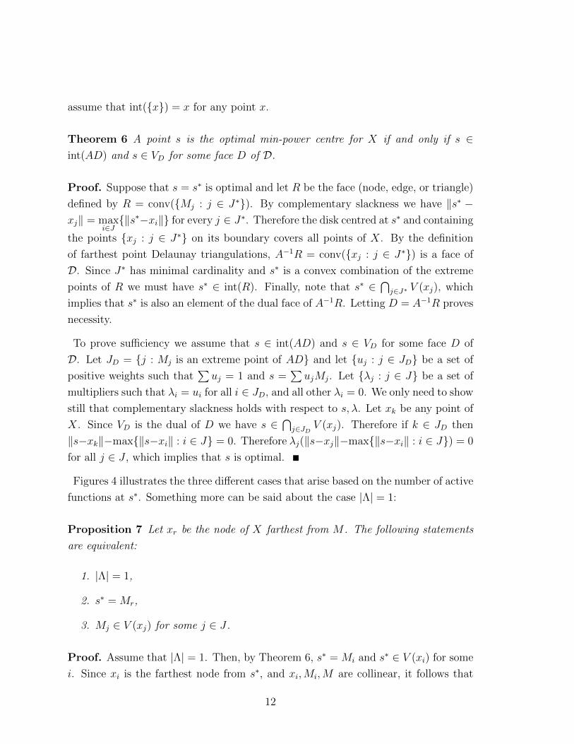
Figures 4 illustrates the three different cases that arise based on the number of active

functions at s∗. Something more can be said about the case |Λ| = 1:

Proposition 7 Let xr be the node of X farthest from M . The following statements

are equivalent:

1. |Λ| = 1,

2. s∗ = Mr,

3. Mj ∈ V (xj) for some j ∈ J .

Proof. Assume that |Λ| = 1. Then, by Theorem 6, s∗ = Mi and s∗ ∈ V (xi) for some

i. Since xi is the farthest node from s∗, and xi,Mi,M are collinear, it follows that

12

VD

=V(xr )

xr=D

s*=Mr=AD

M

(a) |Λ| = 1

DAD

VD

s*

(b) |Λ| = 2

D

s*=VD

(c) |Λ| = 3

Figure 4: Illustrating the three cases of Theorem 6 with |J | = 5. The xj are black-

filled circles, the Mj grey-filled, and s∗ white-filled

13

M ∈ int(V (xi)). Therefore i = r. Finally, suppose that Mj ∈ V (xj) for some j ∈ J .

Then, also by Theorem 6, Mj = s∗. Therefore |Λ| = 1.

Corollary 8 If s∗ ∈ int(V (xj)) for some j ∈ J , then s∗ = Mr.

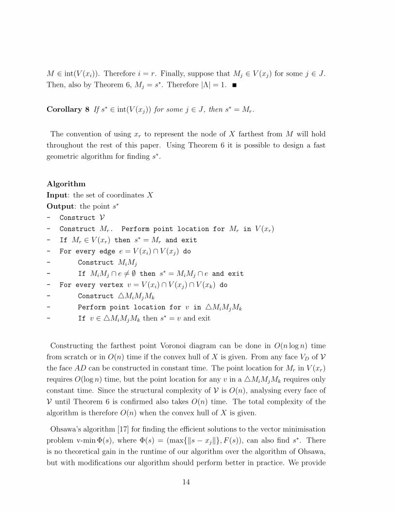
The convention of using xr to represent the node of X farthest from M will hold

throughout the rest of this paper. Using Theorem 6 it is possible to design a fast

geometric algorithm for finding s∗.

Algorithm

Input: the set of coordinates X

Output: the point s∗

- Construct V- Construct Mr. Perform point location for Mr in V (xr)

- If Mr ∈ V (xr) then s∗ = Mr and exit

- For every edge e = V (xi) ∩ V (xj) do

- Construct MiMj

- If MiMj ∩ e 6= ∅ then s∗ = MiMj ∩ e and exit

- For every vertex v = V (xi) ∩ V (xj) ∩ V (xk) do

- Construct 4MiMjMk

- Perform point location for v in 4MiMjMk

- If v ∈ 4MiMjMk then s∗ = v and exit

Constructing the farthest point Voronoi diagram can be done in O(n log n) time

from scratch or in O(n) time if the convex hull of X is given. From any face VD of Vthe face AD can be constructed in constant time. The point location for Mr in V (xr)

requires O(log n) time, but the point location for any v in a 4MiMjMk requires only

constant time. Since the structural complexity of V is O(n), analysing every face of

V until Theorem 6 is confirmed also takes O(n) time. The total complexity of the

algorithm is therefore O(n) when the convex hull of X is given.

Ohsawa’s algorithm [17] for finding the efficient solutions to the vector minimisation

problem v-min Φ(s), where Φ(s) = (max{‖s − xj‖}, F (s)), can also find s∗. There

is no theoretical gain in the runtime of our algorithm over the algorithm of Ohsawa,

but with modifications our algorithm should perform better in practice. We provide

14

an intuitive reason for this as follows. As is well-known, for any set of n points

X the expected number of points that are extreme points of conv(X) is O(log n).

Therefore the expected complexity of the farthest point Voronoi diagram does not

increase very quickly as n increases. Now both M and s∗ are in conv(M), but

conv(M) becomes smaller the more we increase n (note that M is contained in a

disk of radius 1n+1‖M − xr‖). Therefore we suggest that if we modify our algorithm

so that it begins by checking edges and vertices of V close to M , that the expected

number of steps before s∗ is found will be small for large n. In contrast, for a fixed

polygon representing a convex hull, and a fixed point in the polygon representing a

centroid, the cardinality of a set X with this convex hull and centroid will not affect

the practical runtime of Ohsawa’s algorithm. Of course, Ohsawa’s algorithm could

also be modified to begin with points close to M , but his paper presents no theoretical

justification for doing this.

4 The significance of the centroid and the 1-centre

to the min-power centre problem

It is clear from the results so far that the centroid M plays a central role in the

min-power centre problem when α = 2. In particular, it is intuitive that M is always

relatively close to the min-power centre, s∗, since both lie in conv(M). This fact

leads to a theorem at the end of this section which places an upper bound on the

performance ratio of approximating the min-power centre by the centroid. The fact

that M is a “special” point in the min-power centre problem was also observed in

[17], where it is shown that any Parato optimal solution to the vector minimisation

problem v-min Φ(s) lies on a simple path connecting M and the 1-centre of X (recall

that Φ(s) = (Ps, F (s)), where Ps = max{‖s−x‖2 : x ∈ X} and F (s) =∑x∈X

‖s−x‖2).

Interestingly, this path is piecewise linear, consisting of one segment joining M to a

point on an edge of V , and with the remainder of the path lying on the edges of V .

Since the min-power centre is Pareto optimal for v-min Φ(s) it follows that s∗ is also

on this path. This brings us to a second question: what role does the 1-centre play in

the min-power centre problem? We will address this question next before returning

to the discussion on M .

Denote the 1-centre of X by C and letM∗ = {Mj : j ∈ J∗}, where, as before, J∗ is

15

minimal. Therefore s∗ ∈ int(conv(M∗)). The next lemma is given without proof as

it follows from an argument similar to the proof of Theorem 6.

Lemma 9 A point s is the 1-centre of X if and only if s ∈ int(D) and s ∈ VD for

some face D of D.

Proposition 10 If M ∈ conv(M∗) then s∗ = C.

Proof. Clearly |J∗| > 1, since if |J∗| = 1 then s∗ = Mr, but Mr and M are always

distinct. Let X∗ = A−1M∗. Since M ∈ conv(M∗) we have, by Lemma 3, the

fact that conv(M∗) does not intersect the exterior of conv(X∗). Therefore, since

s∗ ∈ int(conv(M∗)) it follows that s∗ ∈ int(conv(X∗)). By letting D = conv(X∗) it

follows from Lemma 9 that s∗ = C as required.

The converse of this result does not appear to hold, but we do have an interesting

corollary.

Corollary 11 M is the min-power centre of X if and only if M and C coincide.

Our final result on the role of C in the min-power centre problem relates to point

sets X that are more or less evenly distributed (with respect to distance) about their

centroid. The proof utilises the formulation of Problem D1′, which, as mentioned be-

fore, is almost exactly the dual of the minimum spanning circle problem except that

the domain of the τj is further restricted by Inequality (5). Note that when α = 2

we can write Equation (7) as s =∑τjxj since

∑τj = 1. Therefore, for α = 2 we have:

Problem D2 (dual of the minimum spanning circle problem).

maximiseτ∈Rn

∑j∈J

τj‖s(τ)− xj‖2

subject to

0 ≤ τj, (11)∑j∈J

τj = 1, (12)

s(τ) =∑j∈J

τjxj. (13)

16

Consider an optimal solution τ ∗ to Problem D2. Therefore s(τ ∗) = C. If τ ∗j ≥ 1n+1

for all j ∈ J then τ ∗ must also be optimal for Problem D1′. By complementary

slackness the fact that τ ∗j ≥ 1n+1

> 0 implies that ‖C − xj‖ − maxi∈J‖C − xi‖ = 0.

Hence all points of X are concyclic about C. To see what the domain restriction

τ ∗j ≥ 1n+1

means geometrically we first need a lemma.

Lemma 12 If there exists affine weights τj ≥ 1n+1

such that s =∑τjxj then s ∈

conv(M).

Proof. If τj ≥ 1n+1

for all j ∈ J then s =∑

1n+1

xj +∑ujxj where uj ≥ 0 and∑

uj = 1n+1

. Let y =

∑ujxj∑uj

= (n + 1)∑ujxj; note that y ∈ conv(X). Hence

s = nn+1

M + 1n+1

y, which implies that ‖s−M‖ = 1n+1‖M − y‖ ≤ 1

n+1‖M − y′‖, where

y′ is on the boundary of conv(X) and M, y, y′ are collinear. The result now follows

from Lemma 3.

The converse of this lemma is not true in general, however, by similar reasoning we

have:

Lemma 13 If s ∈ conv(M) and s is equidistant from all nodes of X then there exists

affine weights τj ≥ 1n+1

such that s =∑τjxj.

Therefore we have the following final result on C, which follows directly from the

above discussion and lemma.

Proposition 14 Suppose that C is equidistant from all points of X. Then C is the

min-power centre of X if and only if C ∈ conv(M).

In some sense it seems we cannot say anything about the location of s∗ without

involving M . In fact, let Q be a polygon with at most n extreme points. For any

point set X with convex hull Q, if there is no restriction on the location of M then

there is no restriction on the location of s∗ (except, of course, that s∗ must lie in Q).

We make this notion clear in the next proposition before closing the section with a

proof that the centroid is a good approximation for the min-power centre.

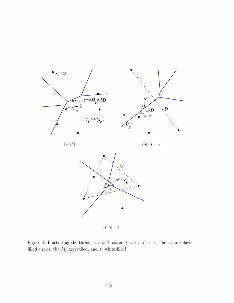
Proposition 15 For any point w ∈ int(conv(X)), where w is on a vertex or edge

of V, there exists a set of points X ′ such that the extreme points of conv(X) and

conv(X ′) coincide and such that the min-power centre of X ′ is w.

17

e

Ma

Mby

M'a

M'bw

xa

xb

M

ε

u

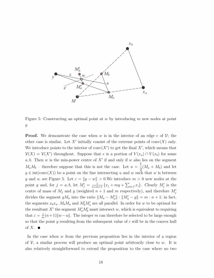
Figure 5: Constructing an optimal point at w by introducing m new nodes at point

y

Proof. We demonstrate the case when w is in the interior of an edge e of V ; the

other case is similar. Let X ′ initially consist of the extreme points of conv(X) only.

We introduce points to the interior of conv(X ′) to get the final X ′, which means that

V(X) = V(X ′) throughout. Suppose that e is a portion of V (xa) ∩ V (xb) for some

a, b. Then w is the min-power centre of X ′ if and only if w also lies on the segment

MaMb – therefore suppose that this is not the case. Let u =1

2(Ma + Mb) and let

y ∈ int(conv(X)) be a point on the line intersecting u and w such that w is between

y and u; see Figure 5. Let ε = ‖y − w‖ > 0.We introduce m > 0 new nodes at the

point y and, for j = a, b, let M ′j = 1

n+m+1

(xj +my +

∑i∈J xi

). Clearly M ′

j is the

centre of mass of Mj and y (weighted n + 1 and m respectively), and therefore M ′j

divides the segment yMa into the ratio ‖Ma −M ′a‖ : ‖M ′

a − y‖ = m : n + 1; in fact,

the segments xbxa, MbMa and M ′bM′a are all parallel. In order for w to be optimal for

the resultant X ′ the segment M ′aM

′b must intersect w, which is equivalent to requiring

that ε = 1m

(n+1)‖w−u‖. The integer m can therefore be selected to be large enough

so that the point y resulting from the subsequent value of ε will be in the convex hull

of X.

In the case when w from the previous proposition lies in the interior of a region

of V , a similar process will produce an optimal point arbitrarily close to w. It is

also relatively straightforward to extend the proposition to the case where no two

18

nodes may coincide, and to the case where all nodes of X ′ are required to lie on the

boundary of the convex hull of X. Any other interesting general restrictions on the

location of s∗ that do not involve M would therefore probably be for sets of nodes

in convex position (i.e., where every node is an extreme point). We leave this as an

open question.

The centroid is very easy to calculate – it can be done in constant time given the

locations of the xj. Corollary 18 shows that M is an appropriate point for approxi-

mating s∗, especially in applications with large n. For any set of points X let

ρ(X) =P (M)

P (s∗).

To place an upper bound on ρ we first need a lemma. Recall once again that xr is

the farthest node from M .

Lemma 16 ‖Mr − xr‖ ≤ ‖s∗ − xr‖.

Proof.

‖xr −M‖ ≤ ‖s∗ − xr‖+ ‖s∗ −M‖ (by the triangle inequality)

≤ ‖s∗ − xr‖+ ‖Mr −M‖ (Mr is the farthest point of

conv(M) from M).

Therefore

‖s∗ − xr‖ ≥ ‖xr −M‖ − ‖Mr −M‖= ‖Mr − xr‖.

Theorem 17 Let k = |arg maxj

{‖s∗ − xj‖}|. Then

ρ(X) ≤ 1

k + 1

(n+ 1

n

)2

+k

k + 1.

Proof. Recall that for any point y we denote by F (y) the sum F (y) =∑j∈J

‖y−xi‖2.

Let xp ∈ X be a farthest node from s∗. By the triangle inequality ‖M − xr‖ ≤‖s∗ −M‖+ ‖s∗ − xr‖ ≤ ‖s∗ −M‖+ ‖s∗ − xp‖.

19

Therefore

‖M − xr‖‖s∗ − xp‖

≤ ‖s∗ −M‖‖s∗ − xp‖

+ 1

≤ ‖Mr −M‖‖s∗ − xr‖

+ 1 (since s∗ ∈M)

≤ ‖Mr −M‖‖Mr − xr‖

+ 1 (by Lemma 16)

=1

n+ 1 =

n+ 1

n(by Lemma 3).

We now have

P (M)

P (s∗)≤ ‖M − xr‖

2 + F (s∗)

‖s∗ − xp‖2 + F (s∗)(since M minimises F )

=‖M − xr‖2 − ‖s∗ − xp‖2

‖s∗ − xp‖2 + F (s∗)+ 1

≤ ‖M − xr‖2 − ‖s∗ − xp‖2

(k + 1)‖s∗ − xp‖2+ 1 (since k longest edges are equal)

=‖M − xr‖2

(k + 1)‖s∗ − xp‖2+

k

k + 1

≤ 1

k + 1

(n+ 1

n

)2

+k

k + 1.

Since k ≥ 1 we conclude that ρ(X) ≤ 1

2

(n+ 1

n

)2

+1

2for any X. The above

approximation is “good” in the following sense. Let Xn be any set of n points.

Corollary 18 limn→∞

ρ(Xn) = 1.

5 A brief look at general α > 1

The situation when α 6= 2 is complicated by the fact that the level curves of the Fj

are no longer circular. In particular, this implies that there are no easily constructed

and useful fixed points directly analogous to the Mj. Even though the farthest point

Voronoi diagram still plays a crucial role for general α, there is no simple dual struc-

ture analogous to the Delaunay triangulation. We may consider arg mins

∑‖s−xj‖α

20

(the generalised Fermat-Weber point) as an analogue for M , however, a compass and

straight-edge construction of this point is almost certainly impossible since even the

classical Fermat-Weber point is not constructible in this way (see [2]).

This section will show, however, that not all insights gained for the α = 2 case are lost

when α 6= 2. In fact, there are several important uses for the mathematical machinery

developed in the preceding sections. Firstly, as discussed in the introduction, path

loss exponents close to α = 2 often occur in real radio network scenarios. It seems

evident that s∗ (and even M) will serve as a good approximation points for min-power

centres based on α close to 2.

Also, some of the the results from the previous section, especially those involving

the 1-centre C, are directly applicable for any α > 1. The conceptual framework that

we present for proving these results consists of transforming the set X into a new set

X(s) such that the general α > 1 min-power centre problem on X is transformed into

the quadratic min-power centre problem on X(s). Preliminary research indicates that

this framework will also be useful for the development of bounds on the performance

of s∗ or the centroid as approximation points for general α.

We first state some notation and a lemma. Recall, from Section 2, that the power

of the star G centred at s with leaf-set X and for a given α is denoted Pα(s,X), and

that Pα(s,X) = maxj∈J{Fα

j (s,X)}. We also similarly generalise the definition of F (s)

to Fα(s,X). The point minimising Pα(s,X) is now denoted by s∗α. Next we describe

the construction of the set X(s). Essentially, each vector xi − s is transformed into

a vector xi(s) − s such that ‖xi − s‖α−1 = ‖xi(s) − s‖. The convex hull of the

resultant set of nodes will therefore contain the convex hull of X when α ≥ 2, with

the inverse of this property holding when α < 2. In formal terms, for any point s let

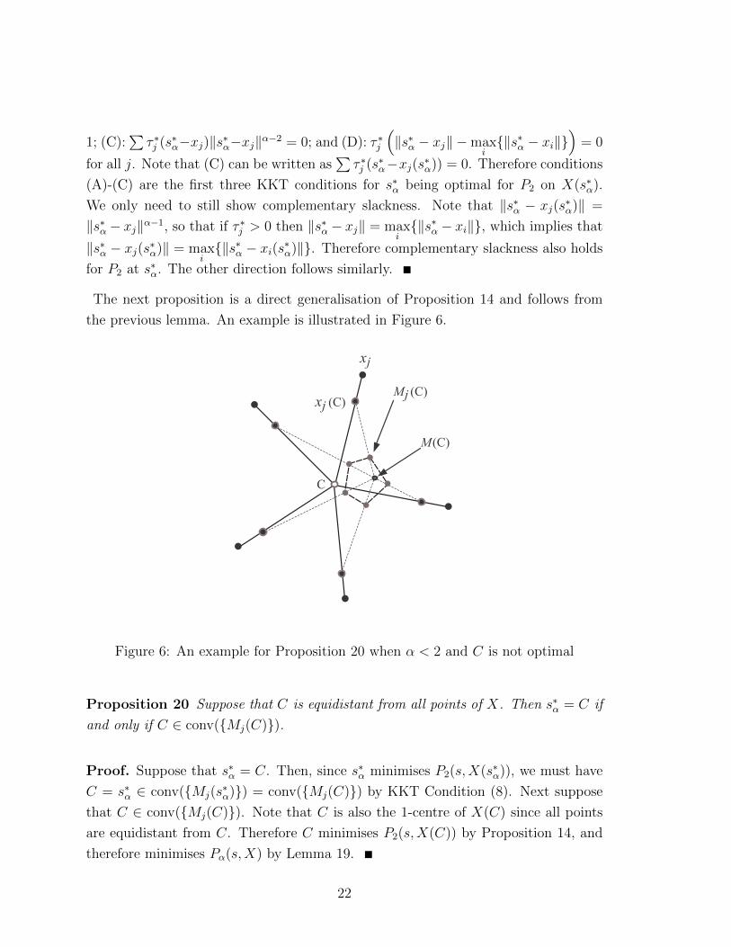
xi(s) = s + ‖s − xi‖α−2(xi − s) and let X(s) = {xj(s) : j ∈ J}. Let M(s) be the

centre of mass of X(s), and let Mj(s) be the j-th 2-centroid of X(s). Some of these

concepts are illustrated in Figure 6 for the set X(s) with s = C and α < 2.

Lemma 19 Let s′ be any point. Then s = s′ minimises P2(s,X(s′)) if and only if

s′ = s∗α.

Proof. Suppose that s′ = s∗α. Since s∗α is optimal for Pα the following KKT conditions

are satisfied: there exist multipliers τ ∗j such that (A):1

n+ 1≤ τ ∗j for all j; (B):

∑τ ∗j =

21

1; (C):∑τ ∗j (s∗α−xj)‖s∗α−xj‖α−2 = 0; and (D): τ ∗j

(‖s∗α − xj‖ −max

i{‖s∗α − xi‖}

)= 0

for all j. Note that (C) can be written as∑τ ∗j (s∗α−xj(s∗α)) = 0. Therefore conditions

(A)-(C) are the first three KKT conditions for s∗α being optimal for P2 on X(s∗α).

We only need to still show complementary slackness. Note that ‖s∗α − xj(s∗α)‖ =

‖s∗α − xj‖α−1, so that if τ ∗j > 0 then ‖s∗α − xj‖ = maxi{‖s∗α − xi‖}, which implies that

‖s∗α − xj(s∗α)‖ = maxi{‖s∗α − xi(s∗α)‖}. Therefore complementary slackness also holds

for P2 at s∗α. The other direction follows similarly.

The next proposition is a direct generalisation of Proposition 14 and follows from

the previous lemma. An example is illustrated in Figure 6.

M (C)

xj

xjM (C)j

(C)

C

Figure 6: An example for Proposition 20 when α < 2 and C is not optimal

Proposition 20 Suppose that C is equidistant from all points of X. Then s∗α = C if

and only if C ∈ conv({Mj(C)}).

Proof. Suppose that s∗α = C. Then, since s∗α minimises P2(s,X(s∗α)), we must have

C = s∗α ∈ conv({Mj(s∗α)}) = conv({Mj(C)}) by KKT Condition (8). Next suppose

that C ∈ conv({Mj(C)}). Note that C is also the 1-centre of X(C) since all points

are equidistant from C. Therefore C minimises P2(s,X(C)) by Proposition 14, and

therefore minimises Pα(s,X) by Lemma 19.

22

This proposition can be strengthened, as shown the following result.

Proposition 21 If s∗2 is equidistant from all point of X then s∗α = s∗2.

Proof. Observe that X(s∗2) is a uniform scaling of X from the point s∗2. Since s∗2minimises P2(s,X) it also minimises P2(s,X(s∗2)). Therefore, by Lemma 19, s∗2 = s∗α.

As a final observation note that as α tends to infinity the longest edge incident to s∗αdominates Fα(s,X). Therefore, since C minimises max{‖s− xj‖α}, and Pα(s,X) =

max{‖s− xj‖α}+ Fα(s,X), we have the following result.

Observation 22 limα→∞

s∗α = C.

6 Conclusion

In this paper we solve the quadratic min-power centre problem in the Euclidean plane.

We provide a complete geometric description and method of construction for the opti-

mal point by means of farthest point Voronoi diagrams. The solution leads to various

structural results relating the min-power centre to the centroid and the 1-centre, and,

in particular, allows us to construct an explicit bound on the performance of the

centroid as an approximation point. We anticipate that the mathematical machinery

developed in this paper will be applied to an important fundamental model for the

physical design of wireless ad hoc networks – namely the geometric range assignment

problem where a bounded number of new nodes may be introduced anywhere in the

plane. Preliminary research has demonstrated that the framework we develop in this

paper will also be useful for problems with cost functions that are not quadratic.

References

[1] Althaus, E., Calinescu, G., Mandoiu, I. I., Prasad, S., Tchervenski, N., & Ze-

likovsky, A. (2006). Power efficient range assignment for symmetric connectivity

in static ad hoc wireless networks. Wireless Networks, 12(3), 287 299.

23

[2] Bajaj, C. (1988). The algebraic degree of geometric optimization problems. Dis-

crete and Computational Geometry, 3(1), 177 191.

[3] Brazil, M., Ras, C.J. & Thomas, D.A. (2012). The bottleneck 2 connected k

Steiner network problem for k ≤ 2. Discrete Applied Mathematics, 160, 1028

1038.

[4] Brazil, M., Ras, C.J. & Thomas, D.A. (2010). Approximating minimum Steiner

point trees in Minkowski Planes, Networks, 56, 244 254.

[5] Brimberg, J., & R. F. Love. (1999). Local convexity results in a generalized

Fermat Weber problem, Computers and Mathematics with Applications, 37(8),

87 97.

[6] Colebrook, M., & Sicilia, J. (2007). A polynomial algorithm for the multicriteria

cent dian location problem. European journal of operational research, 179(3),

1008 1024.

[7] Dhanaraj, M., & Murthy, C. (2007). On achieving maximum network lifetime

through optimal placement of cluster heads in wireless sensor networks. In Pro-

ceedings of IEEE International Conference on Communications, 3142 3147.

[8] Duin, C. W., & Volgenant, A. (2012). On weighting two criteria with a param-

eter in combinatorial optimization problems. European Journal of Operational

Research, 221(1), 1 6.

[9] Dvir, A., & Segal, M. (2010). Placing and maintaining a core node in wireless

ad hoc networks. Wireless Communications and Mobile Computing, 10(6), 826

842.

[10] Elzinga J., Hearn D., & W. Randolph. (1976). Minimax multifacility location

with Euclidean distances, Transportation Science, 10, 321 336.

[11] Eppstein, D. (1992). The farthest point Delaunay triangulation minimizes angles.

Computational Geometry 1(3), 143 148.

[12] Fernandez, F. R., Nickel, S., Puerto, J., & Rodriguez Chıa, A. M. (2001). Ro-

bustness in the Pareto solutions for the multi criteria minisum location problem.

Journal of Multi Criteria Decision Analysis, 10(4), 191 203.

24

[13] Fuchs, B. (2008). On the hardness of range assignment problems. Networks,

52(4), 183 195.

[14] Karl, H., & Willig, A. (2007). Protocols and Architectures for Wireless Sensor

Networks. England: John Wiley & Sons Ltd.

[15] McGinnis, L. F., & White, J. A. (1978). A single facility rectilinear location

problem with multiple criteria. Transportation Science, 12(3), 217 231.

[16] Montemanni, R., Leggieri, V., & Triki, C. (2008). Mixed integer formulations

for the probabilistic minimum energy broadcast problem in wireless networks.

European Journal of Operational Research, 190(2), 578 585.

[17] Ohsawa, Y. (1999). A geometrical solution for quadratic bicriteria location mod-

els. European Journal of Operational Research, 114(2), 380 388.

[18] Paul, B., & Matin, M. A. (2011). Optimal geometrical sink location estimation

for two tiered wireless sensor networks. IET Wireless Sensor Systems, 1(2), 74

84.

[19] Puerto, J., Rodrıguez Chıa, A. M., & Tamir, A. (2010). On the planar piecewise

quadratic 1 Center Problem. Algorithmica, 57(2), 252 283.

[20] Shi, Y., Jia, F., & Hai tao, Y. (2009). An improved router placement algorithm

based on energy efficient strategy for wireless networks. In Proceedings of ISECS

International Colloquium on Computing, Communication, Control, and Man-

agement (IEEE). Vol. 4, 421 423.

[21] Warme, D.M., Winter, P., & Zachariasen, M. (2000). Exact algorithms for steiner

tree problems: a computational study. In D. Du, J. M. Smith, & J. H. Rubinstein

(Eds.), Advances in Steiner trees (pp. 81 116). Netherlands: Kluwer Academic

Publishers.

[22] Yuan, D., & Haugland, D. (2012). Dual decomposition for computational opti-

mization of minimum power shared broadcast tree in wireless networks, IEEE

Transactions on Mobile Computing, 11(12), 2008 2019.

[23] Zhu, Y., Huang, M., Chen, S., & Wang, Y. (2012). Energy efficient topology

control in cooperative ad hoc networks. IEEE Transactions on Parallel and Dis-

tributed Systems, 23(8), 1480 1491.

25