A fresh look at Precision inProcess Conformance

Jorge Munoz-Gama and Josep Carmona

Universitat Politecnica de Catalunya, Spain

jmunoz@lsi.upc.edu, jcarmona@lsi.upc.edu

Abstract. Process Conformance is a crucial step in the area of ProcessMining: the adequacy of a model derived from applying a discovery al-gorithm to a log must be certified before making further decisions thataffect the system under consideration. Among the different conformancedimensions, in this paper we propose a novel measure for precision, basedon the simple idea of counting these situations were the model deviatesfrom the log. Moreover, a log-based traversal of the model that avoidsinspecting its whole behavior is presented. Experimental results show asignificant improvement when compared to current approaches for thesame task. Finally, the detection of the shortest traces in the model thatlead to discrepancies is presented.

Key words: Process Mining, Process Conformance.

1 Introduction and Related Work

Nowadays, the organizations make use of a wide variety of Process-Aware Infor-mation Systems (PAISs) to conduct their business processes [13]. These systemsrecord all kind of information about the processes in logs, which can be used fordifferent purposes. Process Mining is an area of research that aims at the dis-covery, analysis and extension of formal models in a PAIS, in order to supportits design and maintenance.

The problem of deriving a formal model from a log is known as ProcessDiscovery. For this problem, several algorithms exist which derive models thatrepresent (maybe partially) processes detected by observing the traces in thelog. In particular, the production of a Petri net [7] whose underlying behav-ior is related to the traces in the log has been presented extensively in theliterature [17,2,14,4,18]. The Petri nets produced by many of these algorithmsrepresent overapproximations of the log, i.e. the set of traces accepted in the netis a superset of the set of traces in the log. Therefore, one can not rely on theaccuracy of the discovered model unless some minimality property is guaranteed([2,4]), or a certification provided by a metric ensures its quality.

Process Conformance aims at evaluating the adequacy of a model in describ-ing a log. Analyzing conformance is a complex task which involves the interplayof different and orthogonal dimensions [8,9]:

? Fitness: indicates how much of the observed behavior is captured by (i.e.“fits”) the process model.

? Precision: refers to overly general models, preferring models with minimalbehavior to represent as closely as possible the log.

? Generalization: addresses overly precise models which overfit the given log,thus been possible to generalize.

? Structure: refers to models minimal in structure which clearly reflect thedescribed behavior.

Different algorithms for conformance checking have been presented in theliterature (a complete survey can be found in [9]). In particular, some examplesof approaches focused on precision are: [6] (measuring the percentage of potentialtraces in the model that are in the log), [5] (comparing two models and a log to seehow much of the first model’s behavior is covered by the second) used in [14], [19](comparing the behavioral similarity of two models without a log), and [3] (usingminimal description length to evaluate the quality of the model). In this workwe focus on the precision between a model (a Petri net in our case) and a log.On this regard, the methods presented in [10,11] may be seen as a seminal work,were metrics for fitness, structural and precision are presented. In particular,the precision metric presented (called advanced behavioral appropriateness) islimited to comparing the ordering relations between events in the model withthe ones from the log. This approach needs the exhaustive exploration of themodel’s state space, which can be impractical for large models that exhibit ahigh degree of concurrency, i.e. the state-space explosion problem arises.

Briefly, this paper presents a novel technique to measure precision, which aimsat: i) complementing the precision information provided by other techniques, ii)fighting the inherent complexity that relies in checking conformance for industrialor real-life models and logs and, iii) providing useful information for later ProcessExtension, i.e. the stage where the model may be extended to better reflect thelog. The initial implementation is available as the ETConformance plug-in inthe ProM 6 framework [1].

The approach can be summarized as follows:given a model and a log, the behavior of the modelrestricted to the log is computed (part with graybackground in the figure on the right). The bor-der between the log’s and model’s behavior definescrucial points where the model deviates from thelog. We call these situations escaping edges. Byquantifying these edges and their frequency, weaim at providing an accurate measurement of theprecision dimension. Moreover, the escaping edgesdenote inconsistencies that might be treated in theprocess extension phase.

In the previous figure it has been considered that the model’s behavior in-cludes all the log’s behavior (perfect fitness), in order to evaluate its precision.When the fitness condition does not hold, we recommend (as in [10]), to analyse

the conformance in two phases: in the first phase the fitness is evaluated, fil-tering the noise and analysing the discrepancies. In the second phase, the otherthree dimensions are evaluated. Section 7 briefly comments how to deal withnon-fitting models.

1.1 Why a new measure to quantify Precision?

A fresh look at precision We aim at providing a precision metric thatestimates the effort needed to obtain an accurate model, focusing on thediscrepancies detected. This contrasts with the existing approaches for precisionthat only provide discrepancies in the event relations [11].

Efficiency To compute the precision metric, we present a log-based traversalof the model’s behavior . The technique avoids the traversal of the completemodel’s behavior, i.e., only the behavior of the model reflected in the log isexplored (see the figure above). Hence, the approach can handle inputs that cannot be handled by other approaches which traverse the complete behavior.

Granularity The closest measure to the one presented in this paper, is theadvanced behavioral appropriateness, by Rozinat et al [11], denoted by a′B . Thisapproach consists in computing the precedence/follows relations between tasksin the model and in the log, and compares both relations, thus providing abehavioral metric for precision. However, these relations can only have threepossible values: Always, Never and Sometimes. Our approach works directlywith the behavior of the model, getting a deeper view of the precision problem.

Extensionality Finally, we feel that, in addition to the metric, it is importantto provide an appropiate mechanism for the later Process Extension. On thisregard, the methods presented in this paper output also the exact points ofdiscrepancy, i.e., the traces where the model starts to deviate from the log.

The background for the understanding of this paper is presented in Section 2.Section 3 describes informally the approach, whereas Sections 4 and 5 presentthe algorithm to collect escaping edges and the metric for precision analysis,respectively. Section 6 introduces the notion of disconformant traces. Section 7discuss some extensions and experimental results are presented in Section 8.

2 Preliminaries

In this section we present the two main inputs needed to perform the con-formance analysis: Petri nets and logs (Event Logs). Additionally, TransitionsSystems will be presented to link these two inputs.

Some mathematical notation is provided for the understanding of the paper.Given a set S, we denote P(S) as the powerset over S, i.e. the set of possiblesubsets of elements of S. Given a set T , a sequence σ ∈ T ∗ is a called trace.

Given a trace σ = t1t2 . . . tn, and a natural number 0 ≤ k ≤ n, hdk(σ) is thetrace t1t2 . . . tk, also called the prefix of length k in σ. Notice that hd0(σ) = λ,i.e., the empty word. Finally, given a set of traces L, we denote Pref (L) the setof all prefixes for traces in L.

2.1 Petri Nets

Definition 1 (Petri Net [7]). A Petri Net (PN) is a tuple (P, T,W,M0)where P and T represent finite sets of places and transitions, respectively, withP ∩ T = ∅. And W : (P × T ) ∪ (T × P )→ N is the weighted flow relation. Amarking is a mapping P → N. M0 is the initial marking, i.e. defines the initialstate of the system.

A transition t ∈ T is enabled in a marking M iff ∀p ∈ P : M(p) ≥ W (p, t).An enabled transition can be fired resulting in a new marking M ′ such that∀p : M ′(p) = M(p) −W (p, t) + W (t, p). A marking M ′ is reachable from M ifthere is a sequence of firings σ = t1t2 . . . tn that transforms M into M ′, denotedby M [σ〉M ′. A sequence of transitions σ = t1t2 . . . tn is a feasible sequence ifM0[σ〉M , for some M . The set of reachable markings from M0 is denoted by[M0〉, and form a graph called reachability graph. A PN is said to be k-boundedor simply bounded if ∀p : M ′(p) does not exceed a number k for any reachablemarking M ′ from M0. If no such number exists, it is said to be unbounded.

2.2 Event Logs

Event logs contain executions of a system [16]. These executions represent theordering between different tasks, but may also contain additional information,like the task originator or its timestamp. For the purposes of this paper, all thisinformation is abstracted:

Definition 2 (Event Log). An event log EL is a set of traces, i.e., EL ∈ P(T ∗).

We denote by |EL| the number of traces of the log. As notation, these traces canbe iterated through σ1 . . . σ|EL|.

2.3 Relation between a Petri Net and an Event Log

Similarly as it is done in [10], tasks in the log and transitions in the Petri netmust be mapped in order to establish a relation between both objects. Besides themost simple relation between only one task and one transition, the mapping mayhave some more complex scenarios: (i) Duplicate tasks, two or more tasks in themodel are associated with the same task in the log. (ii) Invisible tasks, a task inthe model is associated with no task in the log1. In this paper, the invisible tasks

1 The reasons for this lack of relation may be different: non recordable steps in theprocess (phone calls, meetings, . . . ), introduced in the model for routing purposes,relaxations of the model, or invisible tasks resulting from some discovery algorithm(e.g., [14]).

in the model will be represented as transitions filled black. (iii) Non Modelledtasks, a task in the log is associated with no task in the model. Non modelledtasks are not relevant for the purpose of this paper. Therefore, they can beremoved from the log before starting the analysis. The techniques presented inthis paper cover all the scenarios above. Note that, for the sake of clarity, werefer to task, event or transition indistinctly, whenever no mistake is possible.

2.4 Transitions Systems

Definition 3 (Transition system). A transition system (TS) is a tuple(S, T,A, sin), where S is a set of states, T is an alphabet of actions,A ⊆ S × T × S is a set of (labelled) transitions, and sin ∈ S is the initial state.

We will use se→ s′ as a shortcut for (s, e, s′) ∈ A, and the transitive closure

of this relation will be denoted by∗→. The language of a transition system TS,

L(TS), is the set of traces feasible from the initial state.

3 Problem Statement and Approach

As was said in the introduction, our goal is to measure the precision of a modelwith respect to a log. Moreover, we strive to locate inconsistencies between themodel and the log, thus allowing the later extension of the model.

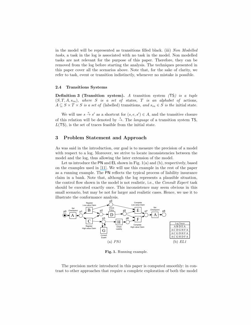
Let us introduce the PN and EL shown in Fig. 1(a) and (b), respectively, basedon the examples used in [11]. We will use this example in the rest of the paperas a running example. The PN reflects the typical process of liability insuranceclaim in a bank. Note that, although the log represents a plausible situation,the control flow shown in the model is not realistic, i.e., the Consult Expert taskshould be executed exactly once. This inconsistence may seem obvious in thissmall scenario, but may be not for larger and realistic cases. Hence, we use it toillustrate the conformance analysis.

(a) PN1 (b) EL1

Fig. 1. Running example.

The precision metric introduced in this paper is computed smoothly: in con-trast to other approaches that require a complete exploration of both the model

and the log [11], in our approach the model exploration is restricted to the ob-served log’s behavior. As a consequence, the computational requirements arebounded to the log size, thus being independent of the whole model’s underlyingbehavior. This might be crucial for models obtained from a mining algorithmthat may have an underlying behavior of intractable size.

The key concept of the approach is that of Escaping Edges, i.e., the situationswere the model allows more behavior than the log, thus exhibiting less precision.We base our measure on the relation between the number and frequency of es-caping edges with respect to model’s behavior restricted to the log . Hence, themore the model deviates from the log, the less precise is its precision value. It isimportant to stress the fact that a model can have few escaping edges (thus ex-hibiting good precision) but with underlying behavior substantially bigger thanthe log: it is not the aim of this work to compare sizes between the model and thelog, but providing an estimation of the efforts required to improve the model toprecisely describe the log. Figure 2 shows the route map of the ETConformanceapproach, and indicates the section where each part is explained in detail.

Fig. 2. Route map of ETConformance: a log and a Petri net are the inputs of thetechnique. Internally, log and Petri net states are identified and mapped. Finally, boththe metric and the set of minimal discrepancies are reported.

4 Log-based Traversal of the Model’s Behavior

This section describes the log-based traversal of the model’s behavior. We havean assumption on the input log: every trace in the log is possible in the model,i.e. it has fitness value one (see how to adapt the technique to non-fitting modelsin Section 7). This assumption is grounded on the correlations that exist betweenfitness and precision dimensions, as pointed in [10]. Hence, the fitness analysisand corresponding adjustments can be done before the precision analysis. Thereare some approaches to perform this task, e.g., [11].

4.1 Basic Idea

In order to perform a log-based traversal of the model behavior, it is necessary tofind a common comparable domain between log and model, i.e. a domain where

1 r,s,sb,p,ac,ap,c

2 r,sb,em,p,ac,ap,c

3 r,sb,p,em,ac,rj,rs,c

4 r,em,sb,p,ac,ap,c

5 r,sb,s,p,ac,rj,rs,c

6 r,sb,p,s,ac,ap,c

7 r,sb,p,em,ac,ap,c

crs

crsacp

rj

crsacp

rj

em

sb

pac ap c

pac ap c

rssb p

sb

sem ac ap c

s ac ap

rj

cem

(b)(a)

Fig. 3. (a) event log EL, (b) corresponding transition system TS such that L(TS) = EL.

states of the model and log states could be mapped. For performing such task,state information must be obtained for both objects (model and log). In the logside, several algorithms are presented in [15] to incorporate state information inthe log. These algorithms are parametrizable with respect to the decision of astate (past, future or both), the representation of the information (sequence, setand multiset), and its horizon (limited or infinite). In particular, using the past,sequence and infinite settings allows to derive a behavioral representation of thelog (a transition system) with the same language. The states of that transitionsystem will be the states of the log.

Definition 4 (Prefix automaton, Log states). Given an event log EL, letTS = (S, T,A, s0) be the automaton derived by using the construction presentedin [15] using the past, sequence and infinite settings. We call this automatonprefix automaton. The set S will be denoted as the set of states of EL. Given atrace σi = t1 . . . t|σi| ∈ EL, sij ∈ S denotes the state in TS corresponding to theprefix t1 . . . tj−1, for 0 ≤ j ≤ |σi|+ 1.

Fig. 3 shows an example of this transformation. The states of this transitionsystem correspond to prefixes of the traces in the log: for instance, the statefilled in Fig. 3 corresponds to the prefix r, sb, p, contained in traces 3, 6 and 7.

To obtain state information for a Petri net model, its reachable states can becomputed. However, due to the well-known space-explosion problem, Petri netscan exhibit a large or even infinite behavior, making this approach impracticalfor these instances. Instead, the approach presented in this paper only visitsthose reachable markings of the net for which there is at least one state in thelog (see Def. 4) mapped. Let us define formally the mapping:

Definition 5 (Mapping between log states and Petri net markings). LetEL and PN = (P, T,W,M0) be a log and a Petri net, respectively, and considerthe prefix automaton TS = (S, T,A, s0) from EL. A marking M is mapped to the

state s ∈ S, denoted by M ( s, if there exists a trace σ such that s0σ→ s in TS

and M0[σ〉M .

Due to this mapping, the Petri net traversal can be controlled to reach onlymarkings for which there is a corresponding mapped state in the log. Moreover,for each one of the markings reached on this guided traversal, the local precision

on this marking can be measured by collecting the discrepancies between thebehavior allowed in the model with respect to the behavior observed in the log:

Definition 6 (Allowed Tasks and Reflected Tasks). Let s be a state of theprefix automaton TS = (S, T,A, s0) from EL, and PN = (P, T,W,M0) a Petri

net. We define AT (s) = {t ∈ T |M ( s ∧ M [t〉M ′} and RT (s) = {t ∈ T | s t→s′)} as the set of allowed and reflected tasks in s.

Since we are assuming fitness value one of the model with respect to the log,clearly RT (s) ⊆ AT (s) for every state s of TS, i.e. the model overapproximatesthe log. Now it is possible to define the concept of escaping edge:

Definition 7 (Escaping Edges). Let s be a state of the prefix automatonTS = (S, T,A, s0) from EL, and PN = (P, T,W,M0) a Petri net. The Escap-ing Edges (EE) of s is defined as EE(s) = AT (s) \RT (s).

An example of escaping edge for the pair (PN1,EL1 ) in Fig. 1 is H in the logstate reached after the prefix AC: here PN1 accepts the H task, whereas this isnot reflected in EL1. It is important to stress that the tasks reflected of a states are the ones that appear in any of the traces that contain s. For instance, forthe example of Fig. 1, the prefix A has two allowed tasks in the model (B andC) but given that both are reflected in the log (in different traces), no escapingedge arise in the log state after observing A. The algorithm to collect the set ofescaping edges is presented as Algorithm. 1.

Input: EL, PNforeach State s in EL do

RT := outEdges (s)σ := prefix (s,EL)mark := fire (σ,PN) // Fire σ and get the reached marking

AT := enable (mark,PN) // Get the enable transitions of markEE := AT \ RT // Allowed tasks minus Reflected Tasks

register (s,EE)

Algorithm 1: ComputeEscapingEdges

4.2 Duplicate and Invisible tasks

Until now, the methods have been explained without considering duplicate orinvisible tasks. Although the approach presented in this paper can deal with du-plicate and invisible tasks, we must remark some issues concerning the potentialindeterminism that may arise.

When trying to determine the marking associated to a log state, it mayhappen that firing the sequence of tasks cannot be done in a deterministic way,i.e., one log task is associated to two or more enabled transitions in the model,

and therefore, one of the transitions must be chosen to continue the firing. Asimilar situation occurs when a sequence of invisible tasks that enables a visiblelog task must be fired. In this cases, part of the state space of the model reachablefrom the current marking must be explored. To avoid producing an infinite statespace (for instance, because the Petri net might be unbounded), we constructthe invisible coverability graph: a variant of the well-known coverability graphalgorithm [7] where the nodes are ω-markings and the edges are only invisibletasks. Informally, this graph will contain all the paths of invisible tasks that leadto the enabling of a visible one. It may occur that a visible task is enabled forseveral and different sequences of invisible tasks, and therefore, a guess betweenthe different sequences must be made to continue the traversal.

In real-life scenarios, dealing with indeterminism requires the use of heuristicsand therefore, the inconsistencies detected (escaping edges in our framework)might be caused by a bad guess and not by a real precision problem. In [11] aheuristic that uses the shortest sequence of invisible that enables a visible taskis proposed. This heuristic tries to minimize the possibility that a invisible firedtask interfere the future firing of another task. In general, the availability ofseveral heuristics can be helpful to apply ad-hoc explorations which depend onthe scenario considered.

5 Evaluating Precision

As it has been seen before, the escaping edges are a good indicator for measuringthe behavior of a model compared to the behavior reflected in the log. For thatreason, we propose a metric to take into account these escaping edges and theirfrequency. This metric also allows us to compare between models to know whichone captures better the behavior reflected of a log. Let us formalize the metric:

Metric 1 (ETC Precision) Let EL = {σ1, . . . , σ|EL|} and PN = (P, T,W,M0)be a log and a Petri net, respectively. For each trace σi (1 ≤ i ≤ |EL|), statesij (1 ≤ j ≤ |σi|+ 1) denotes the j − th state of σi (see Def. 4). The metric isdefined as follows:

etcP (EL,PN) = 1−∑|EL|i=1

∑|σi|+1j=1 |EE(sij)|∑|EL|

i=1

∑|σi|+1j=1 |AT (sij)|

By dividing the set of escaping edges by the set of allowed tasks in the model,the metric evaluates the amount of overapproximation in each trace. Note that,for all sij , |EE(sij)| ≤ |AT (sij)|, and therefore 0 ≤ etcP ≤ 1. The fact that wetake into account the frequency of the traces makes that the most used andappropriate traces would contribute with higher weight than the noisy tracesand the wrong indeterministic choices. The metric value of the example for thepair (PN1, EL1 ) in Fig. 1 is

1− 0 + 3 + 3 + 2

6 + 12 + 13 + 12= 0.81

where every i-th summand of the numerator/denominator is processing the pe-nalizations for the escaping edges of trace σi, e.g., in trace σ4 ∈ EL1 there are 2escaping edges and 12 allowed tasks.

As was done in [10], we present some of the quality requirements a goodmetric should satisfy and a brief justification on its fulfillment.

Validity (The metric and the property to measure must be sufficiently corre-lated with each other). In the case of Metric 1, the more escaping edges, thelower value will be provided (even closer to 0 in the worst case). This inversecorrelation quantifies if a model is a precise description of a log.

Stability (The metric must be as little as possible affected by the properties thatare not measured). In other words, the metric must measure only one dimension(precision in this case) independently of the others (e.g., fitness, structural,generalization). With regard to fitness or generalization, the metric is not stablesince there is a correlation between precision and both dimensions. In contrast,by only focusing on the underlying behavior of the model, etcP is independentto the structural dimension. To illustrate this, Fig.4 show PN2 and PN3, twoPetri Nets with the same behavior and different structure. The result providedby etcP is 1 in both cases when compared with the log EL2.

(a) PN2 (b) EL2 (c) PN3

Fig. 4. Stability of the metric with respect to structure.

Analyzability (It relates to the properties of the measured values. In ourcase, the emphasis is on the requirement that the measured values shouldbe distributed between 0 and 1, with 1 being the best and 0 being the worstvalue. It is important to be 1 when there is no precision problem). The valuesreturned by etcP are distributed between 0 and 1. In addition, the value 1can be reached, indicating that there are no inconsistencies. Notice that, toachieve this value it is not necessary to have only one enabled at each pointof the trace (like in aB [11]). This is because the metric does not depend onthe idea of more enabled tasks, more behavior, but in the concept behaviorallowed vs reflected itself. Moreover, the metric value can be 1, even if the wholebehavior of the model is distributed in two or more different traces. This isbecause decision on escaping edges is done globally after processing the whole setof traces. This can be seen in PN4 and EL3 (cf. Fig. 5), that has a etcP value of 1.

Localizability (The system of measurement forming the metric should be ableto locate those parts in the analyzed object that lack certain measured proper-ties). This is a crucial requirement in conformance analysis, due to the fact that

(a) PN4 (b) EL3

Fig. 5. Global analysis of the traces leads to a global analysis of escaping edges.

providing the discrepancy points we are making possible to identify the poten-tial points of model’s enhancement. This is done in the approach of this paperthrough the escaping edges, identified by their marking and the task used toescape from the reflected behavior in the log. However, given the importance ofthe localizability in conformance, we go a step further and in the next section atechnique to collect the traces leading to these situations is presented.

6 Minimal Disconformant Traces

Given a log and a model, we are interested in identifying these minimal tracesthat lead to a situation where the model starts to deviate from the log. Someof these traces may represent meaningful abstractions that arise in the modeland therefore no further action is required. For the rest of traces, a decisionon whereas the model or the log are wrong shall be made. In the case of anerroneous model, process extension techniques must be applied.

Definition 8 (Minimal Disconformant Traces). Let EL andPN = (P, T,W,M0) be a log and a Petri net, respectively. We define theMinimal Disconformant Traces (MDT) as the set of traces σ = σ′t such thatM0[σ〉M , σ′ ∈ Pref(EL) and σ /∈ Pref(EL).

The escaping edges computed in previous section can be used to obtain theMinimal Disconformant Traces. Algorithm 2 shows how to generate this setof traces using the escaping edges: for each state s with a escaping edge, thesequence to reach s is computed and it is concatenated with the escaping edge.Finally, Lemma 1 ensures a minimality criterion on the derived traces.

Input: ELOutput: Mforeach State s in EL do

foreach Task t in EE(s) doσ := prefix (s,EL)σ := σ · t // Concatenate

addTrace (σ, M) // Register σ as an MDTreturn M

Algorithm 2: ComputeMDT

Lemma 1. Algorithm 2 computes the Minimal Disconformant Traces.

Proof: Let M the set of traces computed by the algorithm ComputeMDT andMDT the set of traces that satisfy Definition 8. To prove M = MDT, we willprove M ⊆ MDT and then MDT ⊆M .

Let σ = σ′t be any trace of M . By construction σ′ is a prefix of the log.However, given the formation of RT and EE in Algorithm 1, σ is not a prefixof the log. Furthermore, σ′ is a feasible sequence of the model because it is aprefix of the log, and all traces in the log are compliant with the model (sincewe assume fitness value one). In addition, by construction of AT and EE , σ is afeasible sequence by the model too. Therefore, σ ∈ MDT.

Now, let σ = σ′t be any trace of MDT. σ′ is a prefix of the log. Accordingto Definition 4, it must be defined a log state s after the sequence σ′. The taskt must be in the AT of s, because σ is a feasible sequence of the model. But tmust not appear in RT because σ is not a prefix of the log. By construction ofRT , t is a Escaping Edge. Therefore, σ ∈M . 2

Fig. 6. MDTs

Following with the running example, Fig. 6 shows theMDTs for the model PN1 and log EL1 (described in Fig. 1).The MDT traces shown are result of the unseen behavior pro-duced by the loop of G, which even allows the possibility ofskipping G. Note that, the set of MDTs computed by Algo-rithm 2 might be seen as a log (i.e sequence of traces). Consequently, all kindof Process Mining techniques can be applied to it in order to get a general viewof the information. In particular, mining methods can be used to obtain a PetriNet representing this extra behavior.

7 Extensions

Log States as Markings The first possible extension is to consider log statesjust as Petri net markings, i.e., two traces reaching the same marking correspondto the same state. With that approach we could have a more high-level vision ofthe precision, e.g., the RT sets of two different states (with the same associatedmarking) now will be united in only one set corresponding to the new state.Although it could be useful in some occasion, we must be awared about all theinformation we are not considering. For instance, the etcP value of (PN1, EL1 )using this new approach would be 1, losing all track about the extra behaviorintroduced by the G loop.

LEEMODEL

LOGEE

Non-fitting models Symmetric to the Escap-ing Edges (EE), we can define the Log EscapingEdges(LEE), i.e., the points where the log deviatesfrom the model. All these points could be evaluated,providing a metric that, in this case, would mesurefitness instead of precision.

All these extensions might be incorporated to extend the applicability of theapproach presented in this paper.

8 Experimental Results

The technique presented in this paper, implemented as the ETConformanceplug-in within ProM 6, has been evaluated on existing public-domain bench-marks [1]. The purpose of the experiments is:

? Justify the existence of a new metric to evaluate precision, i.e. demonstratethe novelty of the concept when compared to previous approaches.

? Show the capacity of the technique to handle large specifications.

Table 1(a) shows a comparison of the technique presented in this paper withthe technique presented in [11], implemented in ProM 5.2 as the ConformanceChecker. The rows in the table represent benchmarks with small size (few traces).The names are shortened, e.g., GFA5 represents GroupedFollowsA5. We reportthe results of checking precision for both conformance checkers in columns un-der a′B and etcP , respectively, for the small Petri nets obtained by the Parikhminer [18] which derived Petri nets with fitness value one. For the case of ourchecker, we additionally provide the number of minimal disconformant traces(|MDT|). We do not report CPU times since checking precision in both ap-proaches took less than one second for each benchmark.

From Table (a) one can see that when the model describes precisely the log,both metrics provide the maximum value. Moreover, when the model is not aprecise description of the log, only three benchmarks provide opposite results(GFBN2, GFl2l, GFl2lSkip). For instance, the GFl2lSkip benchmark a′B is providinga significant lower value: this is because the model contains an optional loopthat is always traversed in the log. This variability is highly penalized by simplyobserving the tasks relations. On the other hand, metric etcP will only penalizethe few situations where the escaping edges appear in the log.

Larger benchmarks for which Conformance Checker cannot handle are pro-vided in Table 1(b). For these benchmarks, we report the results (precision value,number of MDT and CPU time in seconds) for the models obtained by the Parikhminer and the RBMiner [12]. These are two miner that guarantee fitness valueone. For each one of the aN benchmarks, N represents the number of tasksin the log, while the 1 and 5 suffixes denote its size: 100 and 900 traces, re-spectively. The t32 has 200 ( 1) and 1800 ( 5) traces. The pair of CPU timesreported denote the computation of etcP without or with the collection of MDTs(in parenthesis). Also, we provide the results of the most permissive models, i.e.,models with only the transitions but without arcs or places (MT ). These modelsallow any behavior and thus, they have a low etcP value, as expected.

A first conclusion on Table 1 (b) is the capability of handling large bench-marks in reasonable CPU time, even for the prototype implementation carriedout. A second conclusion is the loss of precision of the metric with respect tothe increase of abstraction in the mined models: as soon as the number of tasksincreases, the miners tend to derive models less precise to account for the com-plex relations between different tasks. Often, these miners derive models with ahigh degree of concurrency, thus accepting a potentially exponential number oftraces which might not correspond to the real number of traces in the log.

Table 1. Experimental results for small (a) and big (b) benchmarks.

(a)

Benchmark a′B etcP |MDT| Benchmark a′B etcP |MDT|GFA6NTC 1.00 1.00 0 GFl2lOpt 1.00 0.85 7GFA7 1.00 1.00 0 GFAL2 0.86 0.90 391GFA8 1.00 1.00 0 GFDrivers 0.78 0.89 2GFA12 1.00 1.00 0 GFBN3 0.71 0.88 181GFChoice 1.00 1.00 0 GFBN2 0.59 0.96 19GFBN1 1.00 1.00 0 GFA5 0.50 0.57 35GFParallel5 1.00 0.99 11 GFl2l 0.47 0.75 11GFAL1 1.00 0.88 251 GFl2lSkip 0.30 0.74 10

(b)

MT Parikh RBMiner

Benchmark |TS| etcP |P | |T | etcP |MDT| CPU |P | |T | etcP |MDT| CPU

a22f0n00 1 1309 0.06 19 22 0.63 1490 0(0) 19 22 0.63 1490 0(0)a22f0n00 5 9867 0.07 19 22 0.73 9654 0(3) 19 22 0.73 9654 0(4)a32f0n00 1 2011 0.04 31 32 0.52 2945 0(0) 32 32 0.52 2944 0(1)a32f0n00 5 16921 0.05 31 32 0.59 22750 2(10) 31 32 0.59 22750 2(11)a42f0n00 1 2865 0.03 44 42 0.35 7761 0(2) 52 42 0.37 7228 0(2)a42f0n00 5 24366 0.04 44 42 0.42 60042 5(28) 46 42 0.42 60040 6(29)t32f0n00 1 7717 0.03 30 33 0.37 15064 1(15) 31 33 0.37 15062 1(12)t32f0n00 5 64829 0.04 30 33 0.39 125429 9(154) 30 33 0.39 125429 8(160)

Finally, three charts are provided: the relation between the log size withrespect to the CPU time, the etcP value and the number of MDTs are shownin Fig. 7. For these charts, we selected different log sizes for different types ofbenchmarks (a22f0, a22f5, a32f0,a32f5 for the two bottom charts, a42f0, t32f5and t32f9 for the top chart). For the two bottom charts, we used the Petri netsderived by the Parikh miner to perform the conformance analysis on each log,whereas we use a single Petri net for the top chart to evaluate the CPU time(without collecting MDTs) on different logs, illustrating the linear dependance ofour technique on the log size. The chart on top clearly shows the linear relationbetween log size and CPU time for these experiments, which is expected by thetechnique presented in Sect. 4. The two charts on bottom of the figure show:(left) since for the a22/a32 benchmarks the models derived are very similarindependently of the log, the more traces are included the less escaping edgesare found. On the other hand, the inclusion of more traces contributes to theincorporation of more MDTs, as it is shown in the right chart at the bottom.

9 Conclusion

This paper has presented a low-complexity technique that allows checking theprecision of a general Petri net with respect to a log. By only focusing on theunderlying behavior of the Petri net that is reflected in the log, the technique

0.5

0.55

0.6

0.65

0.7

0.75

0.8

0.85

200 300 400 500 600 700 800 900 1000

etc P

|Log|

etcp vs. Log size

a22f0n00a32f0n00a22f5n00a32f5n00

0

5000

10000

15000

20000

25000

200 300 400 500 600 700 800 900 1000

|MD

T|

|Log|

|MDT| vs. Log size

a22f0n00a32f0n00a22f5n00a32f5n00

Fig. 7. CPU and etcP versus log size for some large benchmarks.

avoids the potential state explosion that might arise when dealing with largeand highly concurrent nets. The theory has been implemented as a plugin withinProM 6 and experimental results are promising. The technique is enriched withthe detection of minimal disconformant traces that may be the starting pointfor extension of the model to better represent the log.

Acknowledgments We would like to thank M. Sole, A. Rozinat and ProMdevelopers for their help. This work has been supported by the project FOR-MALISM (TIN2007-66523), and a grant by Intel Corporation.

References

1. Process mining. www.processmining.org.

2. R. Bergenthum, J. Desel, R. Lorenz, and S.Mauser. Process mining based onregions of languages. In Proc. 5th Int. Conf. on Business Process Management,pages 375–383, Sept. 2007.

3. T. Calders, C. W. Gunther, M. Pechenizkiy, and A. Rozinat. Using minimumdescription length for process mining. In SAC, pages 1451–1455. ACM, 2009.

4. J. Carmona, J. Cortadella, and M. Kishinevsky. A region-based algorithm fordiscovering Petri nets from event logs. In BPM, volume 5240 of LNCS, pages358–373. Springer, 2008.

5. A. K. A. de Medeiros, W. M. P. van der Aalst, and A. J. M. M. Weijters. Quantify-ing process equivalence based on observed behavior. Data Knowl. Eng., 64(1):55–74, 2008.

6. G. Greco, A. Guzzo, L. Pontieri, and D. Sacca. Discovering expressive processmodels by clustering log traces. IEEE Trans. Knowl. Data Eng., 18(8):1010–1027,2006.

7. T. Murata. Petri nets: Properties, analysis and applications. Proceedings of theIEEE, 77(4):541–580, April 1989.

8. A. Rozinat, A. K. A. de Medeiros, C. W. Gunther, A. J. M. M. Weijters, andW. M. P. van der Aalst. The need for a process mining evaluation framework inresearch and practice. In BPM Workshops, volume 4928 of LNCS, pages 84–89,2007.

9. A. Rozinat, A. K. A. de Medeiros, C. W. Gunther, A. J. M. M. Weijters, andW. M. P. van der Aalst. Towards an evaluation framework for process miningalgorithms. BPM Center Report BPM-07-06, BPMcenter. org, 2007.

10. A. Rozinat and W. M. P. van der Aalst. Conformance testing: measuring thealignment between event logs and process models. BETA Working Paper Series,Eindhoven University of Technology, WP 144:203–210, 2005.

11. A. Rozinat and W. M. P. van der Aalst. Conformance checking of processes basedon monitoring real behavior. Information Systems, 33(1):64–95, 2008.

12. M. Sole and J. Carmona. Process mining from a basis of state regions. In Inter-national Conference on Application and Theory of Petri Nets and other Models ofConcurrency (Petri Nets 2010), LNCS. Springer, 2010.

13. W. M. P. van der Aalst. Process-aware information systems: Lessons to be learnedfrom process mining. T. Petri Nets and Other Models of Concurrency, 2:1–26,2009.

14. W. M. P. van der Aalst, A. K. A. de Medeiros, and A. J. M. M. Weijters. Geneticprocess mining. In ICATPN, volume 3536 of LNCS, pages 48–69. Springer, 2005.

15. W. M. P. van der Aalst, V. Rubin, H. M. W. E. Verbeek, B. F. van Dongen,E. Kindler, and C. W. Gunther. Process mining: a two-step approach to balancebetween underfitting and overfitting. Software and Systems Modeling, 2009.

16. W. M. P. van der Aalst, B. F. van Dongen, J. Herbst, L. Maruster, G. Schimm,and A. J. M. M. Weijters. Workflow mining: A survey of issues and approaches.Data Knowl. Eng., 47(2):237–267, 2003.

17. W. M. P. van der Aalst, A. J. M. M. Weijters, and L. Maruster. Workflow mining:Discovering process models from event logs. IEEE Transactions on Knowledge andData Engineering, 16(9):1128–1142, September 2004.

18. J. M. E. M. van der Werf, B. F. van Dongen, C. A. J. Hurkens, and A. Serebrenik.Process discovery using integer linear programming. In Petri Nets, volume 5062 ofLNCS, pages 368–387. Springer, 2008.

19. B. F. van Dongen, J. Mendling, and W. M. P. van der Aalst. Structural patterns forsoundness of business process models. In EDOC, pages 116–128. IEEE ComputerSociety, 2006.