HAL Id: hal-03557760https://hal.archives-ouvertes.fr/hal-03557760

Submitted on 4 Feb 2022

HAL is a multi-disciplinary open accessarchive for the deposit and dissemination of sci-entific research documents, whether they are pub-lished or not. The documents may come fromteaching and research institutions in France orabroad, or from public or private research centers.

L’archive ouverte pluridisciplinaire HAL, estdestinée au dépôt et à la diffusion de documentsscientifiques de niveau recherche, publiés ou non,émanant des établissements d’enseignement et derecherche français ou étrangers, des laboratoirespublics ou privés.

A Formal Model of Interrupt-based Checkpointing withPeripherals

Pierre-Evariste Dagand, Gautier Berthou, Delphine Demange, Tanguy Risset

To cite this version:Pierre-Evariste Dagand, Gautier Berthou, Delphine Demange, Tanguy Risset. A Formal Model ofInterrupt-based Checkpointing with Peripherals. [Technical Report] IRIF; IRISA; INSA RENNES.2022, pp.1-36. �hal-03557760�

A Formal Model of Interrupt-based Checkpointing with Peripherals

GAUTIER BERTHOU, Univ Lyon, INSA-Lyon, Inria, CITI, France

PIERRE-ÉVARISTE DAGAND, Université de Paris, CNRS, France

DELPHINE DEMANGE, Univ Rennes, Inria, CNRS, IRISA, France

RÉMI OUDIN, Sorbonne Univ, CNRS, Inria, LIP6, France

TANGUY RISSET, Univ Lyon, INSA-Lyon, Inria, CITI, France

Transiently-powered systems featuring non-volatile memory as well as external peripherals enable the development of new low-power

sensor applications. However, as programmers, we are ill-equipped to reason about systems where power failures are the norm rather

than the exception. A first challenge consists in being able to capture all the volatile state of the application –external peripherals

included– to ensure progress. A second, more fundamental, challenge consists in specifying how power failures may interact with

peripheral operations. In this paper, we propose a formal specification of intermittent computing with peripherals, an axiomatic

model of interrupt-based checkpointing as well as its proof of correctness, machine-checked in the Coq proof assistant. We state the

correctness of the checkpointing mechanism as a trace refinement property between the model and the specification, which accounts

for peripheral device operations replays due to power failures. Our proof methodology relies on intermediate oracle semantics to tame

the non-determinism of power failures scenarios.

1 INTRODUCTION

Transiently-powered systems are tiny, battery-less devices that harvest energy from their environment. The energy

thus retrieved flows into short-term storage facilities, such as capacitors, leading to computation times on the order

of thousands of cycles per run. A run denotes a continuous period of time without power failure. To ensure progress

of computation across runs, system integrators often pair such devices with non-volatile memory (NVM), such as

non-volatile RAM technology (FRAM, MRAM, etc.). This combination of features gave birth to intermittent computing.

However, the interaction of volatile (registers, caches) and non-volatile states together with unpredictable power failures

is itself a poisonous mix known as the “broken time machine” [37]. This led to the development of programming models

guaranteeing that, at any point in time, the application can be restored to a state where its volatile and non-volatile

components are consistent with each other [9, 32, 42].

An alternative solution to circumvent this issue consists in adding a sensor monitoring the remaining energy

level [16]. Before the power runs out, a hardware interrupt is triggered, which is then handled in software, leading the

system to checkpoint its volatile state to NVM. Checkpoints are necessarily consistent as they result from a snapshot of

the application taken at a single point in time. This offers the simplicity of static checkpointing [32] –where explicit

checkpointing instructions are spread throughout the code– without suffering from the overhead –snapshots are

acquired only when necessary, i.e., when the power runs low. Note that, from a conceptual standpoint, interrupt-based

checkpointing subsumes static checkpointing: in our framework, a static checkpoint is merely a (deterministically-

triggered) power-loss interrupt followed by an immediate reboot to the checkpointed state.

This solution leaves a critical blind spot: external peripheral devices also contain volatile state. However, this state

may not be fully accessible from the CPU –efficiently or at all. Besides, interacting with an external device changes

our expectations about the system. Consider for instance a radio transceiver peripheral. The radio device contains

Authors’ addresses: Gautier Berthou Univ Lyon, INSA-Lyon, Inria, CITI, France; Pierre-Évariste Dagand Université de Paris, CNRS, France; Delphine

Demange Univ Rennes, Inria, CNRS, IRISA, France; Rémi Oudin Sorbonne Univ, CNRS, Inria, LIP6, France; Tanguy Risset Univ Lyon, INSA-Lyon, Inria,

CITI, France.

1

2 Gautier Berthou, Pierre-Évariste Dagand, Delphine Demange, Rémi Oudin, and Tanguy Risset

a frequency synthesizer that must be calibrated before packet emission or reception. Calibration takes about 100`s

on the device, during which the driver is busy-waiting. If a power-loss were to occur after, say, 75`s, it would be

functionally incorrect to resume the transceiver in calibration mode and only wait for the remaining 25`s. To be correct,

the calibration code sequence must execute within a single run.

Following earlier work on supporting peripherals in intermittent computation [2, 7, 10, 18, 36], we identify two key

challenges:

Challenge (C1): Peripherals add volatile and opaque state to the overall system;

Challenge (C2): Peripherals may have a concrete, observable impact on the environment of the system.

The present work aims at providing a conceptual framework for (1) formally expressing these two requirements;

and (2) proving that a general interrupt-based checkpointing scheme meets its specification. To this end, we make the

following assumptions throughout the paper:

Assumption (A1): NVM is solely used to store snapshots of the application. Conversely, application code cannot

access the NVM;

Assumption (A2): Checkpointing volatile state (registers, RAM, etc.) from the micro-controller (MCU) is a solved

problem (e.g., Ahmed et al. [1]) whereas the peripheral internal state is completely opaque to the application;

Assumption (A3): Peripherals act upon an environment that is idempotent. A transiently-powered system may, for

example, send a network packet multiple times: we expect the network protocol to gracefully handle such

situations. This touches upon a fundamental assumption of transiently-powered systems in general [45];

Assumption (A4): Liveness of the application is secured by a suitably calibrated power sensor. We do not assume,

however, that checkpointing always succeeds: we merely expect it to eventually succeed.

While Assumptions (A2) to (A4) are fairly standard assumptions, Assumption (A1) excludes some existing systems [19,

26, 32, 34, 36, 54] from the scope of this work. Since Challenges (C1) and (C2) are orthogonal to an application’s ability

to access NVM, we left out this extension to future work.

Based on these assumptions, we thus propose a general model of interrupt-based checkpointing. This mechanism

has to cope with various failure modes. For example, the device may shut off in the middle of a checkpointing operation,

leaving us with a partial record of the current state of the application. Double-buffering [38] solves this issue: the

previous successful checkpoint is kept at all times. Only when checkpointing completes do we atomically swap the

address of the default checkpoint.

Dealing with an external communication bus (e.g., I2C or SPI), we may for example suffer from a power failure right

after having configured the bus to address a specific component but before actually interacting with the component.

In the next run, the bus will be resumed in its default state: if we resume the application where it lost power, it will

fail to proceed as desired. Instead, one resolves to log the interaction with the peripherals and replay the log upon

reboot [2, 7, 10] so as to drive it to restore its internal state.

Some operations must execute under continuous power to produce a meaningful outcome, as witnessed by our

earlier radio device example. Applications must be able to specify power-continuous sections1asserting that a given

sequence of instructions must be executed within a single run.

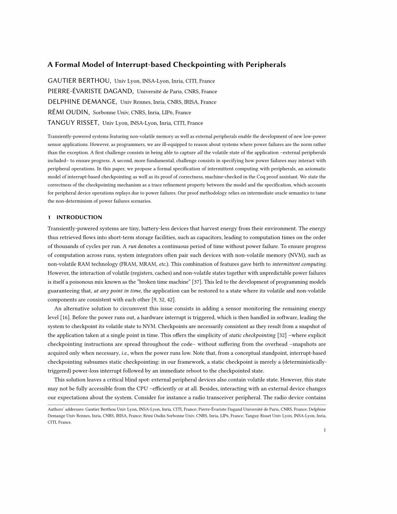
A “correct” system is thus a system that correctly implements each of these techniques as well as their subtle

interactions. Figure 1 gives an overview of our proposal. Our work stems from a specification of the system (SPEC, on

the left-hand side). Power-continuous sections are defined over this model of the application. Peripheral devices (DEV)

1Our notion of “power-continuous section” corresponds to “atomicity” by Maeng and Lucia [36, p.2] and Branco et al. [10, p.6]. We did not follow this

terminology as the term has a (different) meaning in concurrent systems.

A Formal Model of Interrupt-based Checkpointing with Peripherals 3

On-goingcheckpoint

Last validcheckpoint

Power-cont.sections

Applicationmcudev.mcudev.

Periph. API

Power-cont.sections

Application

Periph. API

On-goingcheckpoint

Last validcheckpoint

Power-cont.sections

Applicationmcudev.mcudev.

Periph. API

Power-cont.sections

Application

Periph. API

Fig. 1. Schematic illustration of our model for interrupt-based checkpointing (right) and of its continuous-power specification (left)

are accessed through a specific API that can only be used in a power-continuous section. We then model a general

interrupt-based checkpointing scheme (PLF, on the right-hand side), interacting with peripherals through the same API

and enforcing that power-continuous sections are preserved in the event of a power-loss. To persist state across reboot,

the system uses non-volatile memory (CKP), implementing double-buffering to ensure progress. In particular, a logging

mechanism (LOG) is key to restore peripherals in a consistent state.

Now, this raises the question: formally, what does it mean for our scheme to be correct? The key idea consists in

specifying the application (SPEC in Fig. 1) as if it was run in a continuously-powered environment. Our correctness

result then states that the application supported by a checkpointing scheme behaves as prescribed by SPEC: modulo

the re-execution of some peripherals’ operations, the trace of operations emitted by peripherals is also observable in

the continuous-power specification, and power-continuous sections are executed within a single run.

Our contributions are the following:

• We specify intermittent computing with peripherals (Section 2) with a labeled transition system. We strive for

generality, making no assumption about the actual behavior of peripherals and allowing non-determinism,

including preemptive and concurrent systems.

• We give an axiomatic model of interrupt-based checkpointing (Section 3). To this end, we give an equational

specification of a logging mechanism and a persistent storage interface, thus simplifying the task of checking

the validity of one’s implementation to a handful of conditions. The overall model consists of a state machine

with five states that captures the essence of checkpointing.

• We illustrate our model with existing systems (Section 4). Aside from the pedagogical value of the exercise, this

is also a first step –albeit informal– toward a systematic comparison of checkpointing schemes.

• Finally, we state and prove the correctness of our model with respect to its specification (Section 5). In particular,

we establish that peripheral operations are preserved despite power failures and that power-continuous sections

are indeed complied with.

Overall, the present work aims at consolidating our formal understanding of transiently-powered systems and their

interaction with external peripherals. This is first and foremost a conceptual work. In particular, this paper does not

provide a verification tool nor does it prove the correctness of a particular implementation: our objective is to provide

system designers with a solid, actionable mental model.

All the formal definitions and results presented in this paper have been machine-checked [5] in the Coq proof

assistant [53]. For readability, and for better accessibility from outside of the Coq user community, we have typeset

our Coq definitions using set-theoretic notations. We nonetheless keep a distinct namespace per conceptual object,

which follows the naming scheme NAMESPACE.object. We write NAMESPACE.t to denote abstract components whose

4 Gautier Berthou, Pierre-Évariste Dagand, Delphine Demange, Rémi Oudin, and Tanguy Risset

implementation is left unspecified. Throughout the paper, we use the symbol to relate the following pen-and-paper

constructions with their corresponding mechanized incarnations in our Coq development [5].

Relation to prior publication. This article extends an article that appeared in the proceedings of LCTES 2020 [4].

We extensively illustrate our formal model through examples extracted from the literature (Section 2). We also give

a thorough treatment of the proof techniques involved in our correctness result (Section 5). Our final correctness

theorem is made more precise in the following sense: we establish that our subtrace relation enjoys a unicity property,

guaranteeing that any trace of the PLF machine can be matched with a uniquely determined trace in the SPEC machine.

Finally, we provide an alternative correctness theorem (Section 5.10), where the matching subtrace in the SPECmachine

is explicitly built through an executable version of our (functional) subtrace relation.

2 INTERMITTENT COMPUTING & PERIPHERALS

In the following, we aim to distill the essence of intermittent computing with peripherals. We focus our attention solely

on the challenges raised by the combination of power failure and peripheral devices. To this end, we introduce an

axiomatic programming model. To the practitioner, it may seem far removed from the assembly code that actually

drives intermittent computations. This is in fact a virtue of this work: we aim at providing a conceptual framework

with which to reason about intermittent computations and their interaction with peripherals. By freeing ourselves from

a particular implementation, we remain non-prescriptive about orthogonal design choices, such as the treatment of

concurrency, interrupts, etc. We thus offer a very liberal specification that can be readily and effectively used to reason

about the design of a concrete implementation.

In this section, we layout our specification of intermittent computations, which ought to be met by our checkpointing

model. We encourage readers to check that the behaviors they care about in their applications can be captured by our

specification.

2.1 Modeling the MCU

We specify the MCU [ ] as an overarching abstraction of the CPU registers and relevant fragments of volatile memory

(RAM). It encompasses all the volatile states that can efficiently be checkpointed to NVM through standard techniques [3].

It does not include peripheral devices –whose treatment comes next– and non-volatile memory –which is outside the

scope of our specifications, as per Assumption (A1). In the following, we letMCU.t be the set of possible MCU states.

We use the variable mcu ∈ MCU.t to denote an arbitrary MCU state. We call MCU.init ∈ MCU.t the initial MCU state,

just before executing the first instruction of a given application.

Example 1 (MSP430FR series microcontroller). Sytare [7] and Karma [10] have been successfully deployed on a Texas

Instruments MSP430FR5739 MCU. Similar controllers have been used in the literature (either MSP430FR5994 [36], or

MSP430FR5739 [2]).

The state of the 16-bit MSP430 processor (16 registers, including program counter, stack pointer, status register and

constant generator) as well as its 4 KB of RAM and its code memory (including the read-only bootloader) define an

instance of MCU.t. Its initial stateMCU.init is specified in the user manual (e.g., [21, §1.2.1]). ■

2.2 Modeling peripheral devices

We present now, under the DEV [ ] namespace, our model of peripheral device. Handling Challenge (C1) calls for a

careful distinction between the physical peripherals –whose internal state cannot be accessed by the program– and the

A Formal Model of Interrupt-based Checkpointing with Peripherals 5

interface it exposes to the program. We therefore introduce both an abstract description of the peripheral, representing

the state of the physical device, and an interface driving the evolution of the abstract device state.

We let DEV.t be the set of possible physical peripheral states, and use the variable dev ∈ DEV.t to denote an arbitrary

peripheral state. We call DEV.init ∈ DEV.t the initial peripheral state, on power-up.

Example 2 (MSP430FR series microcontroller). Sytare has shown that the following on-board devices can be supported

through a checkpointing mechanism:

• clock system (CS) [20, §6.10.2][48]

• general input/output (GPIO) [20, §6.10.3][49]

• SPI bus [20, §6.10.7][50]

• 8-channel 10-bit analog-to-digital converter (ADC), including the temperature sensor [20, §6.10.12][51]

• 16-bit timers [20, §6.10.8][52]

as well as an external Texas Instruments CC2500 2.4 GHz RF transceiver [23, 47] connected via SPI. The overall state

represented by this collection of devices defines an instance of DEV.t. Their initial state, as specified by the datasheets,

defines a distinguished initial state DEV.init.

Karma [10] has pushed further the study of external devices connected to this MCU, supporting the following

devices:

• Knowles SPW2430HR5H [27] analog microphone connected via the TLV voltage comparator of the MCU

• Sensirion Temperature/Humidity Sensor SHT11 [41] connected via I2C

• Microchip RN42 Bluetooth radio [41] connected via UART

• Intersil ISL29004 [24] light sensors connected via I2C

• Texas Instruments CC1101 sub-GHz RF transceiver [22] connected via SPI

• ST LIS3MDL 3-axis magnetometer [43] connected via SPI

• ST LSM6DSL 3-axis accelerometer/gyroscope [44] connected via I2C

■

The idea that peripherals are manipulated through a well-defined interface is a natural one [10]. It may involve the

low-level application binary interface (ABI) documented by a datasheet or the application program interface (API)

provided by a high-level library. We accommodate either style by assuming that there exists a set DEV.request of

requests supported by the peripheral. For any given request q? ∈ DEV.request, there exists a set DEV.response covering

the possible responses (i.e., returned values) of the peripheral. Given a particular device state, performing a request

has the effect of emitting some response and producing a new device state. The behavior of a peripheral can thus be

specified through a relation

− −↦→−{DEV

− ⊆ DEV.t × DEV.request × DEV.response × DEV.t

where dev

q? ↦→r

!

{DEV

dev′denotes the execution of a query q

?in device state dev that resulted in a response r

!and led to

device state dev′. This relation thus plays an essential role in our formalization. It turns requests to devices, over which

the software has control, into actions on the physical device DEV.t, over which the software has no control.

A pair of a request and its corresponding response form an operation. Formally we define DEV.ops ≜ DEV.request ×DEV.response. Conventionally, we write op ∈ DEV.ops to denote an arbitrary pair of request and response q

? ↦→ r!.

6 Gautier Berthou, Pierre-Évariste Dagand, Delphine Demange, Rémi Oudin, and Tanguy Risset

Our simple modeling of peripheral devices accounts for systems featuring multiple physically-decoupled peripherals.

We can simply consider the set of all available devices as a single one whose interface is the disjoint sum of their

respective interfaces.

In the following, we flesh out this abstract notion with concrete interfaces from the literature (Example 3 to 7). The

corresponding Coq model can be found by following the suitable link but we shall not dwell on the specifics of each

implementation, which is overall unsurprising.

Example 3 (Sytare API: temperature sensor [ ]). In Sytare, applications access devices through a designated “system

call” interface. For example, the temperature sensor (part of the ADC component) is presented as a single function that

encapsulates both sensor calibration as well as the actual measurement:

int temp_sample ();

The temperature sensor is thus exposed as a read-only, stateless interface. ■

Example 4 (Sytare API: sub-main clock [ ]). Conversely, the sub-main clock (SMCLK, part of the clock system) provides

a stateful interface:

int clk_set_smclk_src (clock_src_t source );

clock_src_t clk_get_smclk_src ();

int clk_set_smclk_div (clock_div_t divisor );

clock_div_t clk_get_smclk_div ();

carrying the assumption that the usual semantics of getter/setter pairs is preserved across runs, i.e., a getter retrieves

the value that was last and successfully set. ■

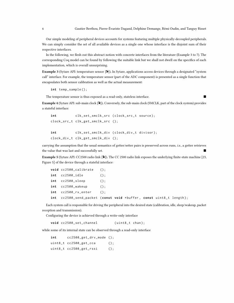
Example 5 (Sytare API: CC2500 radio link [ ]). The CC 2500 radio link exposes the underlying finite-state machine [23,

Figure 5] of the device through a stateful interface:

void cc2500_calibrate ();

int cc2500_idle ();

int cc2500_sleep ();

int cc2500_wakeup ();

int cc2500_rx_enter ();

int cc2500_send_packet (const void *buffer , const uint8_t length );

Each system call is responsible for driving the peripheral into the desired state (calibration, idle, sleep/wakeup, packet

reception and transmission).

Configuring the device is achieved through a write-only interface

void cc2500_set_channel (uint8_t chan);

while some of its internal state can be observed through a read-only interface

int cc2500_get_drv_mode ();

uint8_t cc2500_get_cca ();

uint8_t cc2500_get_rssi ();

A Formal Model of Interrupt-based Checkpointing with Peripherals 7

■

Remark. As discussed in Branco et al. [10, §3.1, “Peripheral APIs”], Karma has adopted a similar, coarse-grained

interface definition. The exact API is not specified in the publication and the implementation is not publicly available.

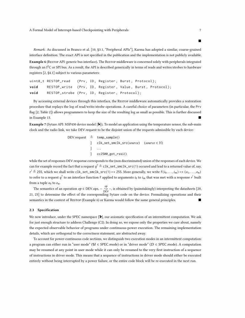
Example 6 (Restop API: generic bus interface). The Restopmiddleware is concerned solely with peripherals integrated

through an I2C or SPI bus. As a result, the API is described generically in terms of reads and writes/strobes to hardware

registers [2, §4.1] subject to various parameters:

uint8_t RESTOP_read (Prv , ID, Register , Burst , Protocol );

void RESTOP_write (Prv , ID, Register , Value , Burst , Protocol );

void RESTOP_strobe (Prv , ID, Register , Protocol );

By accessing external devices through this interface, the Restop middleware automatically provides a restoration

procedure that replays the log of read/write/strobe operations. A careful choice of parameters (in particular, the Prv

flag [2, Table 2]) allows programmers to keep the size of the resulting log as small as possible. This is further discussed

in Example 13. ■

Example 7 (Sytare API: MSP430 device model [ ]). To model an application using the temperature sensor, the sub-main

clock and the radio link, we take DEV.request to be the disjoint union of the requests admissible by each device:

DEV.request ≜ temp_sample()⊎ clk_set_smclk_src(𝑠𝑜𝑢𝑟𝑐𝑒) (𝑠𝑜𝑢𝑟𝑐𝑒 ∈ N)⊎ . . .

⊎ cc2500_get_rssi()

while the set of responsesDEV.response corresponds to the (non discriminated) union of the responses of each device.We

can for example record the fact that a request q? ≜ clk_set_smclk_src(1) occured and lead to a returned value of, say,

r! ≜ 255, which we shall write clk_set_smclk_src(1) ↦→ 255. More generally, we write f(𝑖0, . . . , 𝑖𝑚) ↦→ (𝑜1, . . . , 𝑜𝑛)to refer to a request q

?to an interface function f applied to arguments 𝑖0 to 𝑖𝑚 that was met with a response r

!built

from a tuple 𝑜0 to 𝑜𝑛 .

The semantics of an operation op ∈ DEV.ops, −op

{DEV

−, is obtained by (painstakingly) interpreting the datasheets [20,

21, 23] to determine the effect of the corresponding Sytare code on the device. Formalizing operations and their

semantics in the context of Restop (Example 6) or Karma would follow the same general principles. ■

2.3 Specification

We now introduce, under the SPEC namespace [ ], our axiomatic specification of an intermittent computation. We ask

for just enough structure to address Challenge (C2). In doing so, we expose only the properties we care about, namely

the expected observable behavior of programs under continuous-power execution. The remaining implementation

details, which are orthogonal to the correctness statement, are abstracted away.

To account for power-continuous code sections, we distinguish two execution modes in an intermittent computation:

a program can either run in “user mode” (U ∈ SPEC.mode) or in “driver mode” (D ∈ SPEC.mode). A computation

may be resumed at any point in user mode while it can only be resumed to the very first instruction of a sequence

of instructions in driver mode. This means that a sequence of instructions in driver mode should either be executed

entirely without being interrupted by a power failure, or the entire code block will be re-executed in the next run.

8 Gautier Berthou, Pierre-Évariste Dagand, Delphine Demange, Rémi Oudin, and Tanguy Risset

Example 8. The calibration code of the radio frequency synthesizer (discussed in the introduction) should therefore be

specified as a driver mode code sequence. This ensures that the busy-wait is always executed as a whole before calibration

is deemed completed. Other examples include non-immediate transactions, frequent with SPI or I2C buses. ■

Modes are thus a key ingredient to specify power-continuous sections. We write m ∈ SPEC.mode to denote an

arbitrary execution mode.

Our specification should be able to describe a set of desired behaviors. Since peripherals are meant to interact with

their environment, a natural notion of “behavior” is the sequence of operations performed by the device. We write

SPEC.trace ≜ DEV.ops∗ for the set of sequences of operations. We write t ∈ SPEC.trace to denote an arbitrary trace,

𝜖 to denote the empty sequence and t ; t′to denote a concatenation of traces. We define dev

t

{DEV

∗dev

′ ≜ dev

op0

{DEV

dev0 . . .op𝑛{DEV

dev′, the sequential execution of the trace t = op

0; . . . ; op𝑛 starting from device state dev, resulting in

device state dev′.

Intermittent computations are described axiomatically. The state of the computation

SPEC.state ≜ SPEC.mode ×MCU.t × DEV.t

consists of a mode, an MCU state and a device state. We write s ∈ SPEC.state to denote an arbitrary state. The execution

of a program is specified through a single-step transition relation − −{

SPEC− ⊆ SPEC.state × SPEC.trace × SPEC.state

that takes an input state to produce a (possibly empty) trace of observable events and a resulting state.

This relation is subject to the following invariants.

(Axiom-Usr): In user mode, computations do not interact with peripherals, i.e., if

(U,mcu, dev) t

{SPEC

(U,mcu′, dev′),

then dev = dev′and t = 𝜖 ;

(Axiom-Drv): In driver mode, the emitted trace faithfully describes the physical evolution of the device, i.e., if

(D,mcu, dev) t

{SPEC

(D,mcu′, dev′),

then dev

t

{DEV

∗dev

′;

(Axiom-Enter): Transitions from user to driver mode are computationally transparent, i.e., if

(U,mcu, dev) t

{SPEC

(D,mcu′, dev′),

then mcu = mcu′, dev = dev

′and t = 𝜖 ;

(Axiom-Leave): Transitions from driver to user mode are computationally transparent, i.e., if

(D,mcu, dev) t

{SPEC

(U,mcu′, dev′),

then mcu = mcu′, dev = dev

′and t = 𝜖 .

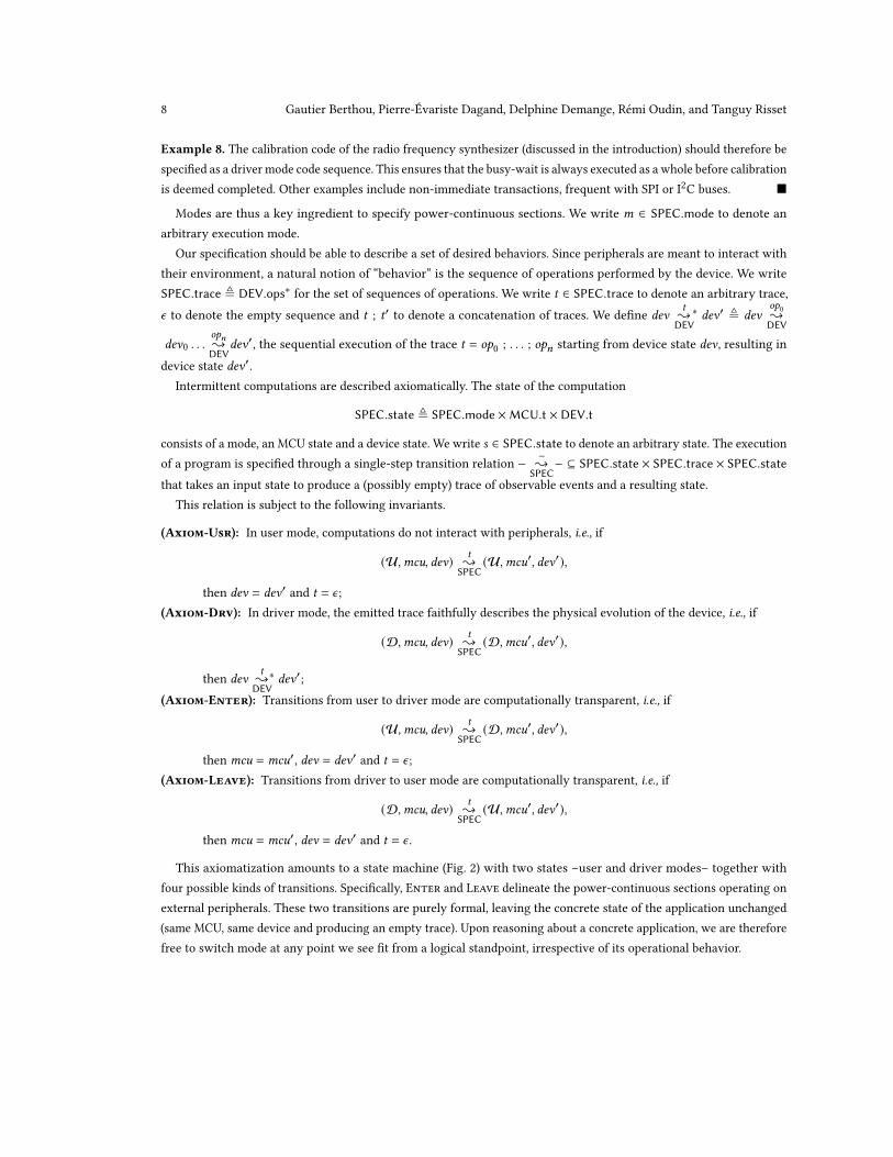
This axiomatization amounts to a state machine (Fig. 2) with two states –user and driver modes– together with

four possible kinds of transitions. Specifically, Enter and Leave delineate the power-continuous sections operating on

external peripherals. These two transitions are purely formal, leaving the concrete state of the application unchanged

(same MCU, same device and producing an empty trace). Upon reasoning about a concrete application, we are therefore

free to switch mode at any point we see fit from a logical standpoint, irrespective of its operational behavior.

A Formal Model of Interrupt-based Checkpointing with Peripherals 9

(U,mcu, dev) (D,mcu, dev)Usr Drv

Enter

Leave

Fig. 2. Specification state machine

The semantics of an intermittent computation follows simply by iterating the single-step transition relation above,

starting from the initial state. Formally, we define the semantics SPEC.sem as the following set of traces:

𝑡 ∈ SPEC.sem ⇔ ∃s, (U,MCU.init,DEV.init) t

{SPEC

∗s

The set SPEC.sem consists of all the admissible behaviors of the system under study. Indeed, any trace in this set

corresponds to a sequence of peripheral operations performed during a continuously-powered execution.

Being a specification, the above definition of SPEC.sem deserves scrutiny. In particular, it must be expressive enough

to account for the properties expected by a specific, real-world application. To fit within our framework, these properties

need to be expressible in terms of traces specifying expected observations, and/or user-driver transitions specifying

power-continuous sections. The following examples illustrate how our specification addresses Challenge (C2).

Example 9. Suppose we want to (1) sense a temperature through temp_sample() (Example 3), then (2) convert that

value to a human-readable format to (3) be sent over the wireless link through cc2500_send_packet (Example 5). This

program can be modeled either as a single sequence encompassing all three operations executing in mode D, or as

three sequences executing in, successively, D → U → D modes, value conversion being performed in modeU. In

both cases, the formal trace consists in a sensing operation followed by a send operation. However, the latter case

describes an application that –subject to power failures– allows for the temperature sent over the air to be arbitrarily

outdated, whereas the former case captures the timeliness requirement of the whole sequence of operations. ■

Example 10 (Interrupt support). Consider an application that regularly sends an external sensor’s data in radio packets.

The application sets a timer to periodically sense and send data, then waits for commands from the radio between

packet emissions. If both the sensor and the radio devices are accessed through the same SPI bus, this SPI bus requires

two different configurations (e.g., bus clock frequency), both being distinct operations in DEV.ops, to communicate

with both devices.

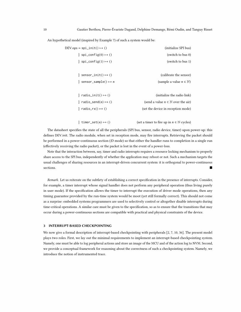
10 Gautier Berthou, Pierre-Évariste Dagand, Delphine Demange, Rémi Oudin, and Tanguy Risset

An hypothetical model (inspired by Example 7) of such a system would be:

DEV.ops = spi_init() ↦→ () (initialize SPI bus)

⊎ spi_config(0) ↦→ () (switch to bus 0)

⊎ spi_config(1) ↦→ () (switch to bus 1)

⊎ sensor_init() ↦→ () (calibrate the sensor)

⊎ sensor_sample() ↦→ 𝑛 (sample a value 𝑛 ∈ N)

⊎ radio_init() ↦→ () (initialize the radio link)

⊎ radio_send(𝑛) ↦→ () (send a value 𝑛 ∈ N over the air)

⊎ radio_rx() ↦→ () (set the device in reception mode)

⊎ timer_set(𝑛) ↦→ () (set a timer to fire up in 𝑛 ∈ N cycles)

The datasheet specifies the state of all the peripherals (SPI bus, sensor, radio device, timer) upon power-up: this

defines DEV.init. The radio module, when set in reception mode, may fire interrupts. Retrieving the packet should

be performed in a power-continuous section (D mode) so that either the handler runs to completion in a single run

(effectively receiving the radio packet), or the packet is lost in the event of a power-loss.

Note that the interaction between, say, timer and radio interrupts requires a resource locking mechanism to properly

share access to the SPI bus, independently of whether the application may reboot or not. Such a mechanism targets the

usual challenges of sharing resources in an interrupt-driven concurrent system: it is orthogonal to power-continuous

sections. ■

Remark. Let us reiterate on the subtlety of establishing a correct specification in the presence of interrupts. Consider,

for example, a timer interrupt whose signal handler does not perform any peripheral operation (thus living purely

in user mode). If the specification allows the timer to interrupt the execution of driver mode operations, then any

timing guarantee provided by the run-time system would be moot (yet still formally correct). This should not come

as a surprise: embedded systems programmers are used to selectively control or altogether disable interrupts during

time-critical operations. A similar care must be given to the specification, so as to ensure that the transitions that may

occur during a power-continuous sections are compatible with practical and physical constraints of the device.

3 INTERRUPT-BASED CHECKPOINTING

We now give a formal description of interrupt-based checkpointing with peripherals [2, 7, 10, 36]. The present model

plays two roles. First, we lay out the minimal requirements to implement an interrupt-based checkpointing system.

Namely, one must be able to log peripheral actions and store an image of the MCU and of the action log to NVM. Second,

we provide a conceptual framework for reasoning about the correctness of such a checkpointing system. Namely, we

introduce the notion of instrumented trace.

A Formal Model of Interrupt-based Checkpointing with Peripherals 11

3.1 Operation logging

To restore a physical device into a previously encountered state, we must resort to the only information accessible to

the program: peripheral operations, i.e., the requests sent to the device and their respective responses. In this section,

we consider an abstract specification of an operation logging mechanism, under the namespace LOG [ ]. Below, and in

Section 4, we show that this interface admits several efficient implementations.

We let LOG.t to be the summary of all previous peripheral operations. An operation can be added to a given log

through the function LOG.log ∈ DEV.ops → LOG.t → LOG.t. Restoring the log, through the function LOG.restore ∈LOG.t → DEV.t, ought to recreate a peripheral state ex nihilo by interpreting the log. We denote LOG.init ∈ LOG.t

the initial state of the log. We write ℓ ∈ LOG.t to denote an arbitrary log. We require that function LOG.restore be

consistent with LOG.init and LOG.log:

(Axiom-Restore-Init) Restoring the initial log yields the initial state, i.e.,

LOG.restore LOG.init = DEV.init

(Axiom-Restore-Log) Given a log that faithfully represents a given device, restoring the extension of this log

with a new operation gives the same peripheral state as the one obtained by running the operation on the

peripheral, i.e., for all ℓ ∈ LOG.t, dev, dev′ ∈ DEV.t, op ∈ DEV.ops, if LOG.restore ℓ = dev and dev

op

{DEV

dev′,

then LOG.restore (LOG.log op ℓ) = dev′.

We overload notations and write LOG.log t ℓ for the sequential logging of each individual operation of a trace

t = op0

; . . . ; op𝑛 , i.e., LOG.log op𝑛 (. . . (LOG.log op0LOG.init)).

Remark. While similar in appearance, the notion of trace t ∈ SPEC.trace (Section 2.3) and the above axiomatic model

of logs ℓ ∈ LOG.t live at two distinct conceptual levels. Traces, on the one hand, are purely logical objects, which let us

specify and reason about the behaviors of programs. Logs, on the other hand, model a computer artifact, namely the

mechanism by which the state of external peripherals is given an in-memory representation (to enable storage to NVM,

as described in the following Section).

Remark. This specification makes no assumption concerning the determinism (or lack thereof) of the underlying

device hardware. The relational nature of ourmodel of devices (Section 2.2) accommodates the fact that a given peripheral

request may non-deterministically yield a specific peripheral response and internal state. However, logging an operation

through LOG.log amounts to recording both the request and its response. As a consequence, the statement of Axiom

(Axiom-Restore-Log) is careful to consider only those device states dev′that are induced by the same operation, that is

the same pair of request and response. Formally, we are thus carefully side-stepping the non-determinism of responses.

Indeed, the role of the logging mechanism is to re-create a specific state, which was the result of a specific sequence of

requests and responses: we need not account for all possible responses, only those that occurred during the execution

whose final state we intend to recreate.

Non-example 11. The statement of (Axiom-Restore-Log) hints at the fact that some devices may nonetheless exhibit

too much non-determinism to support a logging mechanism. Let us consider a device state dev, a specific request q?and

its corresponding response r!such that there exists two internal device states dev𝑎 ≠ dev𝑏 satisfying both

dev

q? ↦→r

!

{DEV

dev𝑎 and dev

q? ↦→r

!

{DEV

dev𝑏

12 Gautier Berthou, Pierre-Évariste Dagand, Delphine Demange, Rémi Oudin, and Tanguy Risset

meaning that the physical device is allowed to (silently) pick an internal state over which the software interface has no

visibility. It should come as no surprise that such kind of device cannot be reliably used in the setting of intermittent

computing: if we had to reboot after the execution of the operation q? ↦→ r

!, we would be unable to decide whether to

restore the device to dev𝑎 or dev𝑏 . ■

Read contrapositively, this non-example yields a necessary condition for a peripheral to be compatible with in-

termittent computing: for any device state dev ∈ DEV.t, any pair of a request q? ∈ DEV.request and a response

r! ∈ DEV.response, there exists at most one device state dev

′satisfying dev

q? ↦→r

!

{DEV

dev′. That is, the device response r

!

must reflect all the non-determinism of the peripheral.

Example 12. Let us consider the application depicted in Example 10. Assume that the sensor module and the radio

module respectively require the SPI bus configurations 0 (spi_config(0)) and 1 (spi_config(1)), we would, for

example, record the interaction

ℓ = LOG.log (radio_send(42) ↦→ ())

(LOG.log (spi_config(1) ↦→ ())

(LOG.log (sensor_sample() ↦→ 42)

(LOG.log (spi_config(0) ↦→ ())

(LOG.log (radio_init() ↦→ ())

(LOG.log (spi_config(1) ↦→ ())

(LOG.log (sensor_init() ↦→ ())

(LOG.log (spi_config(0) ↦→ ())

(LOG.log (spi_init() ↦→ ())

LOG.init)))))))))

which reads from the inside out as starting from the initial state –represented by LOG.init– we record a spi_init

operation, followed by a call to spi_config, followed by a call to sensor_init, etc. Starting back from the initial device

state (as is the case after a reboot), the log ℓ contains all the necessary information to restore the devices in a coherent

state, as per our assumption (Axiom-Restore-Log). In particular, we are guaranteed that the sensor and the radio

modules are accessed through a correctly configured SPI bus, independently of the fact that a reboot has occurred and

that the SPI bus has been reinitialized.

Remark that LOG.log need not actually store the full record of interactions. For instance, the effect of the last call to

spi_config supersedes the effect of any earlier call to spi_config: we may therefore only log the trace of this last

call, overwriting previous occurrences. This is the key idea behind the log implementation of Restop (Example 13).

Similarly, the operation sensor_sample() need not be stored in the log: reading a sensor has no impact on the

sensor’s state. There is no point in re-executing this operation upon reboot. Exploiting detailed knowledge of the

semantics of operations enables Sytare and Karma to tailor their log representation to a static, fixed-size datastructure

(Example 14). ■

Example 13 (Restop: compressed log). Arreola et al. [2, §4.3] describes a mechanism to systematically minimize the

size of logs. Restop operations (Example 6) carry a Prv flag that indicates whether they need to be saved in the log or

A Formal Model of Interrupt-based Checkpointing with Peripherals 13

not, and whether they overwrite any preceding occurrence or not. While, formally, the resulting log can be seen as an

unbounded list of read, write and strobe operations, this extra semantics information allow –in practice– to compress

the log as it is populated. ■

Example 14 (Sytare device context & Karma state machine). Berthou et al. [7, §3.2.1] introduce the notion of “device

context” to record the state of a device in memory. The device context is manually crafted by the driver developer and

is assumed to faithfully account for the physical state of the device: each operation modifying the peripheral state is

responsible for updating the device context accordingly. Branco et al. [10, §4] follows the same approach through the

notion of driver “state machine”.

Device contexts can be understood as an aggressively compact implementation of LOG.log, exploiting semantic

knowledge of the device behavior to provide a fixed-sized representation of the peripheral state (the device context

datastructure). While Restop offers the Prv flag for the driver developer to hint at some of the semantics of operations

(which is then used to dynamically compact the log of operations), a driver developer for Sytare or Karma is given full

power to optimize the representation of the peripheral state. For instance, Karma driver developers are advised that

“synchronous calls need not create new states unless they change the peripheral configuration” (Branco et al. [10, p.4]):

indeed, an operation that does not modify the state of the peripheral (e.g.,, sampling a stateless sensor) need not be

logged and, therefore, there is no need to allocate space for it in the device context or driver state machine. ■

3.2 Non-volatile checkpoint storage

Checkpointing storage is the only component in our system that is persistent across reboots. We formalize it under

the namespace CKP [ ]. Non-volatile checkpoints are represented by an abstract set CKP.t. Intuitively, a checkpoint

contains two snapshots of the application, implementing double-buffering [38]: a stable one (the “last” valid one) and an

on-going one (the “next” valid one, if checkpointing succeeds). A snapshot consists of an MCU image and a peripheral

log. We write ckp ∈ CKP.t to denote an arbitrary checkpointing storage.

We access the last snapshot through the function last ∈ CKP.t → MCU.t × LOG.t, and the next snapshot through

next ∈ CKP.t → MCU.t × LOG.t. For conciseness, we also define lastMcu, lastLog, nextMcu and nextLog to directly

access each individual component. The initial checkpoint CKP.init ∈ CKP.t is constructed from the image of the

initial MCU and the initial log, i.e., it satisfies the equations last CKP.init = (MCU.init, LOG.init) and next CKP.init =

(MCU.init, LOG.init).Double-buffering requires two operations. First, one must be able to overwrite atomically the last stable snapshot with

the on-going one, effectively committing the on-going snapshot. This is provided by functionCKP.set ∈ CKP.t → CKP.t.

Second, one must be able to overwrite atomically the on-going snapshot with the last valid one, effectively resetting the

on-going snapshot to the last valid one. This is provided by CKP.reset ∈ CKP.t → CKP.t. These functions are specified

through a set of equations:

last (CKP.set ckp) = next ckp(overwrite the last snapshot with the on-going one)

next (CKP.set ckp) = next ckp

next (CKP.reset ckp) = last ckp(reset the on-going snapshot to the last one)

last (CKP.reset ckp) = last ckp

Finally, one must be able to update the MCU image or the log stored in the next snapshot. This is respectively

achieved by function CKP.saveNextMcu ∈ CKP.t → MCU.t → CKP.t and function CKP.saveNextLog ∈ CKP.t →

14 Gautier Berthou, Pierre-Évariste Dagand, Delphine Demange, Rémi Oudin, and Tanguy Risset

INIT (USR,mcu, dev, ckp) (DRV,mcu, dev, ckp, ℓ)

(PWR, ckp)

(OFF, ckp)

First-Boot

Enter

Usr

Leave

UsrPwr DrvPwr

Drv

UsrOff DrvOff

Ckp-Succ

Ckp-FailReboot

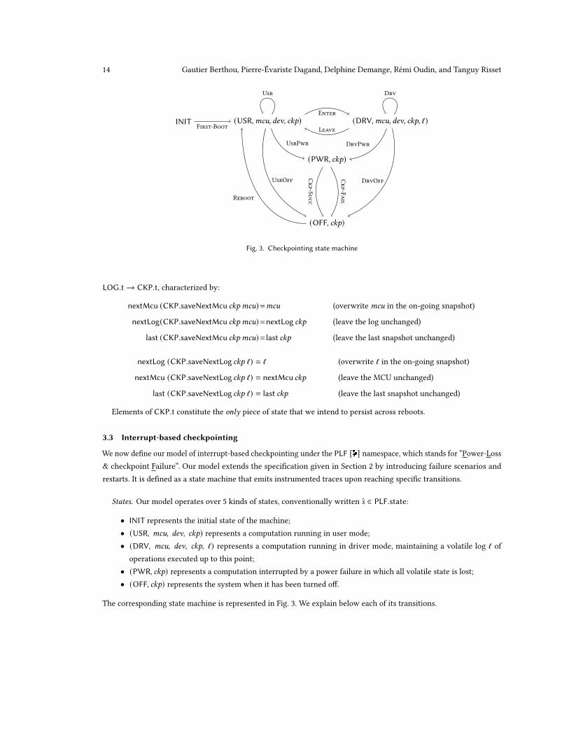
Fig. 3. Checkpointing state machine

LOG.t → CKP.t, characterized by:

nextMcu (CKP.saveNextMcu ckp mcu)=mcu (overwrite mcu in the on-going snapshot)

nextLog(CKP.saveNextMcu ckp mcu)=nextLog ckp (leave the log unchanged)

last (CKP.saveNextMcu ckp mcu)= last ckp (leave the last snapshot unchanged)

nextLog (CKP.saveNextLog ckp ℓ) = ℓ (overwrite ℓ in the on-going snapshot)

nextMcu (CKP.saveNextLog ckp ℓ) = nextMcu ckp (leave the MCU unchanged)

last (CKP.saveNextLog ckp ℓ) = last ckp (leave the last snapshot unchanged)

Elements of CKP.t constitute the only piece of state that we intend to persist across reboots.

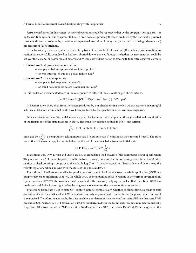
3.3 Interrupt-based checkpointing

We now define our model of interrupt-based checkpointing under the PLF [ ] namespace, which stands for “Power-Loss

& checkpoint Failure”. Our model extends the specification given in Section 2 by introducing failure scenarios and

restarts. It is defined as a state machine that emits instrumented traces upon reaching specific transitions.

States. Our model operates over 5 kinds of states, conventionally written s ∈ PLF.state:

• INIT represents the initial state of the machine;

• (USR, mcu, dev, ckp) represents a computation running in user mode;

• (DRV, mcu, dev, ckp, ℓ) represents a computation running in driver mode, maintaining a volatile log ℓ of

operations executed up to this point;

• (PWR, ckp) represents a computation interrupted by a power failure in which all volatile state is lost;

• (OFF, ckp) represents the system when it has been turned off.

The corresponding state machine is represented in Fig. 3. We explain below each of its transitions.

A Formal Model of Interrupt-based Checkpointing with Peripherals 15

Instrumented traces. In this system, peripheral operations could be repeated either by the program –during a run– or

by the run-time system –due to a power failure. In order to relate precisely the trace produced by the transiently-powered

system with a trace produced by a continuously-powered execution of the system, it is crucial to distinguish (repeated)

progress from failed attempts.

In the transiently-powered system, we must keep track of two kinds of information: (1) whether a power-continuous

section has successfully completed or has been aborted due to a power failure; (2) whether the next snapshot could be

set over the last one, or power ran out beforehand. We thus extend the notion of trace with four extra observable events:

Information 1: A power-continuous section

• completed before a power-failure interrupt: Log⊤

• or was interrupted due to a power failure: Log⊥

Information 2: The checkpointing

• completed before power ran out: Ckp⊤

• or could not complete before power ran out: Ckp⊥

In this model, an instrumented trace is thus a sequence of either of these events or peripheral actions:

t ∈ PLF.trace ≜ ({Ckp⊤,Ckp⊥, Log⊤, Log⊥} ⊎ DEV.ops)∗

In Section 5, we show that, from the traces produced by our checkpointing model, we can extract a meaningful

subtrace of DEV.ops events that could have been produced by the specification, i.e., within a single run.

State machine transitions. Wemodel interrupt-based checkpointing with peripherals through a relational specification

of the transitions of the state machine in Fig. 3. The transition relation defined in Fig. 4, and written

− −{PLF

− ⊆ PLF.state × PLF.trace × PLF.state

indicates by s

t

{PLF

s′a computation taking input state s to output state s

′emitting an instrumented trace t. The trace

semantics of the overall application is defined as the set of traces reachable from the initial state:

t ∈ PLF.sem ⇔ ∃s, INIT t

{PLF

∗s

Transitions Usr, Drv, Enter and Leave are key to embedding the behavior of the continuous-power specification.

They mirror their SPEC counterparts, in addition to retrieving (transition Enter) or storing (transition Leave) infor-

mation to checkpointing storage, or to the volatile log (Drv). Crucially, transitions Enter, Drv and Leave keep the

volatile log of operations in sync with the state of the physical device.

Transitions to PWR are responsible for producing a consistent checkpoint across the whole application (MCU and

peripherals). Upon transition UsrPwr, the whole MCU is checkpointed so as to resume at the current program point.

Upon transition DrvPwr, the volatile execution context is thrown away, relying on the fact that transition Enter has

produced a valid checkpoint right before leaving user mode to enter the power-continuous section.

Transitions from state PWR to state OFF capture, non-deterministically, whether checkpointing succeeds or fails

(transitions Ckp-Succ and Ckp-Fail). We also allow cases where power could run out before the power-failure interrupt

is even raised. Therefore, in user mode, the state machine non-deterministically steps from stateUSR to either state PWR

(transition UsrPwr) or stateOFF (transition UsrOff). Similarly, in driver mode, the state machine non-deterministically

steps from DRV to either state PWR (transition DrvPwr) or state OFF (transitions DrvOff). Either way, when the

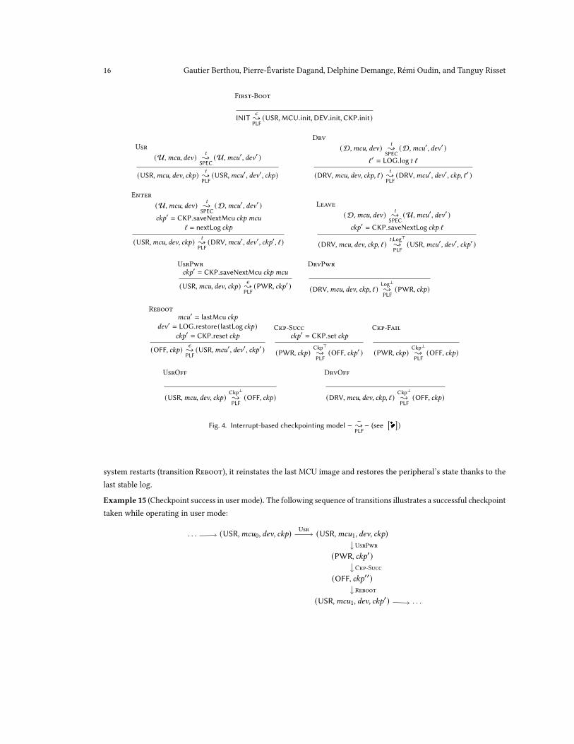
16 Gautier Berthou, Pierre-Évariste Dagand, Delphine Demange, Rémi Oudin, and Tanguy Risset

First-Boot

INIT𝜖{PLF

(USR,MCU.init,DEV.init,CKP.init)

Usr

(U,mcu, dev) t

{SPEC

(U,mcu′, dev′ )

(USR,mcu, dev, ckp) t

{PLF

(USR,mcu′, dev′, ckp)

Drv

(D,mcu, dev) t

{SPEC

(D,mcu′, dev′ )

ℓ ′ = LOG.log t ℓ

(DRV,mcu, dev, ckp, ℓ ) t

{PLF

(DRV,mcu′, dev′, ckp, ℓ ′ )

Enter

(U,mcu, dev) t

{SPEC

(D,mcu′, dev′ )

ckp′ = CKP.saveNextMcu ckp mcu

ℓ = nextLog ckp

(USR,mcu, dev, ckp) t

{PLF

(DRV,mcu′, dev′, ckp′, ℓ )

Leave

(D,mcu, dev) t

{SPEC

(U,mcu′, dev′ )

ckp′ = CKP.saveNextLog ckp ℓ

(DRV,mcu, dev, ckp, ℓ )t;Log⊤{PLF

(USR,mcu′, dev′, ckp′ )

UsrPwr

ckp′ = CKP.saveNextMcu ckp mcu

(USR,mcu, dev, ckp) 𝜖{PLF

(PWR, ckp′ )

DrvPwr

(DRV,mcu, dev, ckp, ℓ )Log⊥{PLF

(PWR, ckp)

Reboot

mcu′ = lastMcu ckp

dev′ = LOG.restore(lastLog ckp)

ckp′ = CKP.reset ckp

(OFF, ckp) 𝜖{PLF

(USR,mcu′, dev′, ckp′ )

Ckp-Succ

ckp′ = CKP.set ckp

(PWR, ckp)Ckp⊤{PLF

(OFF, ckp′ )

Ckp-Fail

(PWR, ckp)Ckp⊥{PLF

(OFF, ckp)

UsrOff

(USR,mcu, dev, ckp)Ckp⊥{PLF

(OFF, ckp)

DrvOff

(DRV,mcu, dev, ckp, ℓ )Ckp⊥{PLF

(OFF, ckp)

Fig. 4. Interrupt-based checkpointing model − −{PLF

− (see[ ]

)

system restarts (transition Reboot), it reinstates the last MCU image and restores the peripheral’s state thanks to the

last stable log.

Example 15 (Checkpoint success in user mode). The following sequence of transitions illustrates a successful checkpoint

taken while operating in user mode:

. . . (USR,mcu0, dev, ckp) (USR,mcu1, dev, ckp)

(PWR, ckp′)

(OFF, ckp′′)

(USR,mcu1, dev, ckp′) . . .

Usr

UsrPwr

Ckp-Succ

Reboot

A Formal Model of Interrupt-based Checkpointing with Peripherals 17

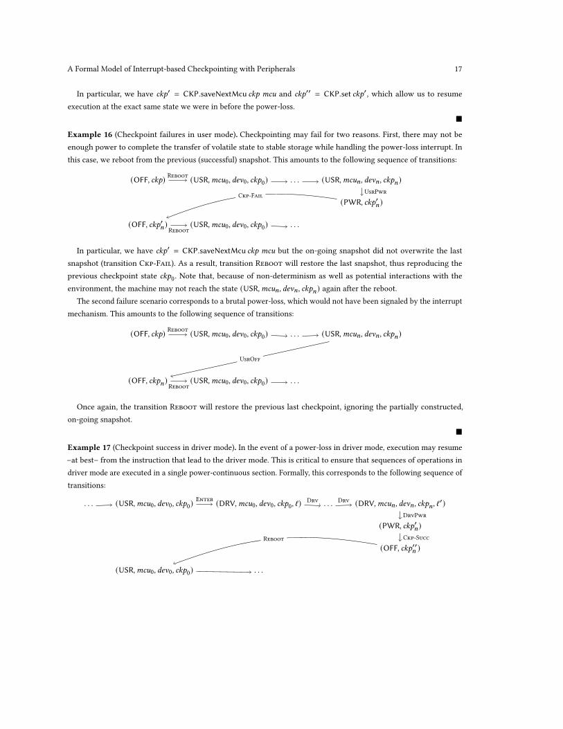
In particular, we have ckp′ = CKP.saveNextMcu ckp mcu and ckp

′′ = CKP.set ckp′, which allow us to resume

execution at the exact same state we were in before the power-loss.

■

Example 16 (Checkpoint failures in user mode). Checkpointing may fail for two reasons. First, there may not be

enough power to complete the transfer of volatile state to stable storage while handling the power-loss interrupt. In

this case, we reboot from the previous (successful) snapshot. This amounts to the following sequence of transitions:

(OFF, ckp) (USR,mcu0, dev0, ckp0) . . . (USR,mcu𝑛, dev𝑛, ckp𝑛)

(PWR, ckp′𝑛)

(OFF, ckp′𝑛) (USR,mcu0, dev0, ckp0) . . .

Reboot

UsrPwr

Ckp-Fail

Reboot

In particular, we have ckp′ = CKP.saveNextMcu ckp mcu but the on-going snapshot did not overwrite the last

snapshot (transition Ckp-Fail). As a result, transition Reboot will restore the last snapshot, thus reproducing the

previous checkpoint state ckp0. Note that, because of non-determinism as well as potential interactions with the

environment, the machine may not reach the state (USR,mcu𝑛, dev𝑛, ckp𝑛) again after the reboot.

The second failure scenario corresponds to a brutal power-loss, which would not have been signaled by the interrupt

mechanism. This amounts to the following sequence of transitions:

(OFF, ckp) (USR,mcu0, dev0, ckp0) . . . (USR,mcu𝑛, dev𝑛, ckp𝑛)

(OFF, ckp𝑛) (USR,mcu0, dev0, ckp0) . . .

Reboot

UsrOff

Reboot

Once again, the transition Reboot will restore the previous last checkpoint, ignoring the partially constructed,

on-going snapshot.

■

Example 17 (Checkpoint success in driver mode). In the event of a power-loss in driver mode, execution may resume

–at best– from the instruction that lead to the driver mode. This is critical to ensure that sequences of operations in

driver mode are executed in a single power-continuous section. Formally, this corresponds to the following sequence of

transitions:

. . . (USR,mcu0, dev0, ckp0) (DRV,mcu0, dev0, ckp0

, ℓ) . . . (DRV,mcu𝑛, dev𝑛, ckp𝑛, ℓ′)

(PWR, ckp′𝑛)

(OFF, ckp′′𝑛 )

(USR,mcu0, dev0, ckp0) . . .

Enter Drv Drv

DrvPwr

Ckp-SuccReboot

18 Gautier Berthou, Pierre-Évariste Dagand, Delphine Demange, Rémi Oudin, and Tanguy Risset

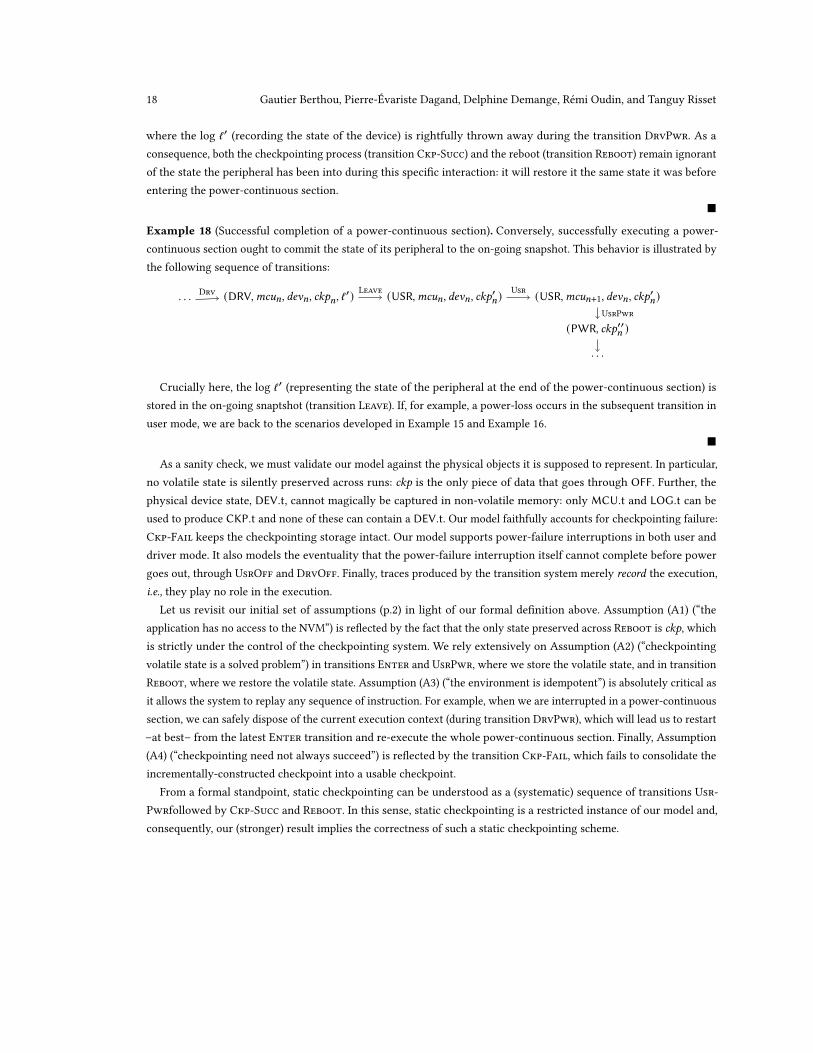
where the log ℓ′ (recording the state of the device) is rightfully thrown away during the transition DrvPwr. As a

consequence, both the checkpointing process (transition Ckp-Succ) and the reboot (transition Reboot) remain ignorant

of the state the peripheral has been into during this specific interaction: it will restore it the same state it was before

entering the power-continuous section.

■

Example 18 (Successful completion of a power-continuous section). Conversely, successfully executing a power-

continuous section ought to commit the state of its peripheral to the on-going snapshot. This behavior is illustrated by

the following sequence of transitions:

. . . (DRV,mcu𝑛, dev𝑛, ckp𝑛, ℓ′) (USR,mcu𝑛, dev𝑛, ckp

′𝑛) (USR,mcu𝑛+1, dev𝑛, ckp

′𝑛)

(PWR, ckp′′𝑛 )

. . .

Drv Leave Usr

UsrPwr

Crucially here, the log ℓ′ (representing the state of the peripheral at the end of the power-continuous section) is

stored in the on-going snaptshot (transition Leave). If, for example, a power-loss occurs in the subsequent transition in

user mode, we are back to the scenarios developed in Example 15 and Example 16.

■

As a sanity check, we must validate our model against the physical objects it is supposed to represent. In particular,

no volatile state is silently preserved across runs: ckp is the only piece of data that goes through OFF. Further, the

physical device state, DEV.t, cannot magically be captured in non-volatile memory: only MCU.t and LOG.t can be

used to produce CKP.t and none of these can contain a DEV.t. Our model faithfully accounts for checkpointing failure:

Ckp-Fail keeps the checkpointing storage intact. Our model supports power-failure interruptions in both user and

driver mode. It also models the eventuality that the power-failure interruption itself cannot complete before power

goes out, through UsrOff and DrvOff. Finally, traces produced by the transition system merely record the execution,

i.e., they play no role in the execution.

Let us revisit our initial set of assumptions (p.2) in light of our formal definition above. Assumption (A1) (“the

application has no access to the NVM”) is reflected by the fact that the only state preserved across Reboot is ckp, which

is strictly under the control of the checkpointing system. We rely extensively on Assumption (A2) (“checkpointing

volatile state is a solved problem”) in transitions Enter and UsrPwr, where we store the volatile state, and in transition

Reboot, where we restore the volatile state. Assumption (A3) (“the environment is idempotent”) is absolutely critical as

it allows the system to replay any sequence of instruction. For example, when we are interrupted in a power-continuous

section, we can safely dispose of the current execution context (during transition DrvPwr), which will lead us to restart

–at best– from the latest Enter transition and re-execute the whole power-continuous section. Finally, Assumption

(A4) (“checkpointing need not always succeed”) is reflected by the transition Ckp-Fail, which fails to consolidate the

incrementally-constructed checkpoint into a usable checkpoint.

From a formal standpoint, static checkpointing can be understood as a (systematic) sequence of transitions Usr-

Pwrfollowed by Ckp-Succ and Reboot. In this sense, static checkpointing is a restricted instance of our model and,

consequently, our (stronger) result implies the correctness of such a static checkpointing scheme.

A Formal Model of Interrupt-based Checkpointing with Peripherals 19

4 INSTANCES OF THE MODEL

We now relate our model to propositions from the literature, illustrating how they fit within our conceptual framework.

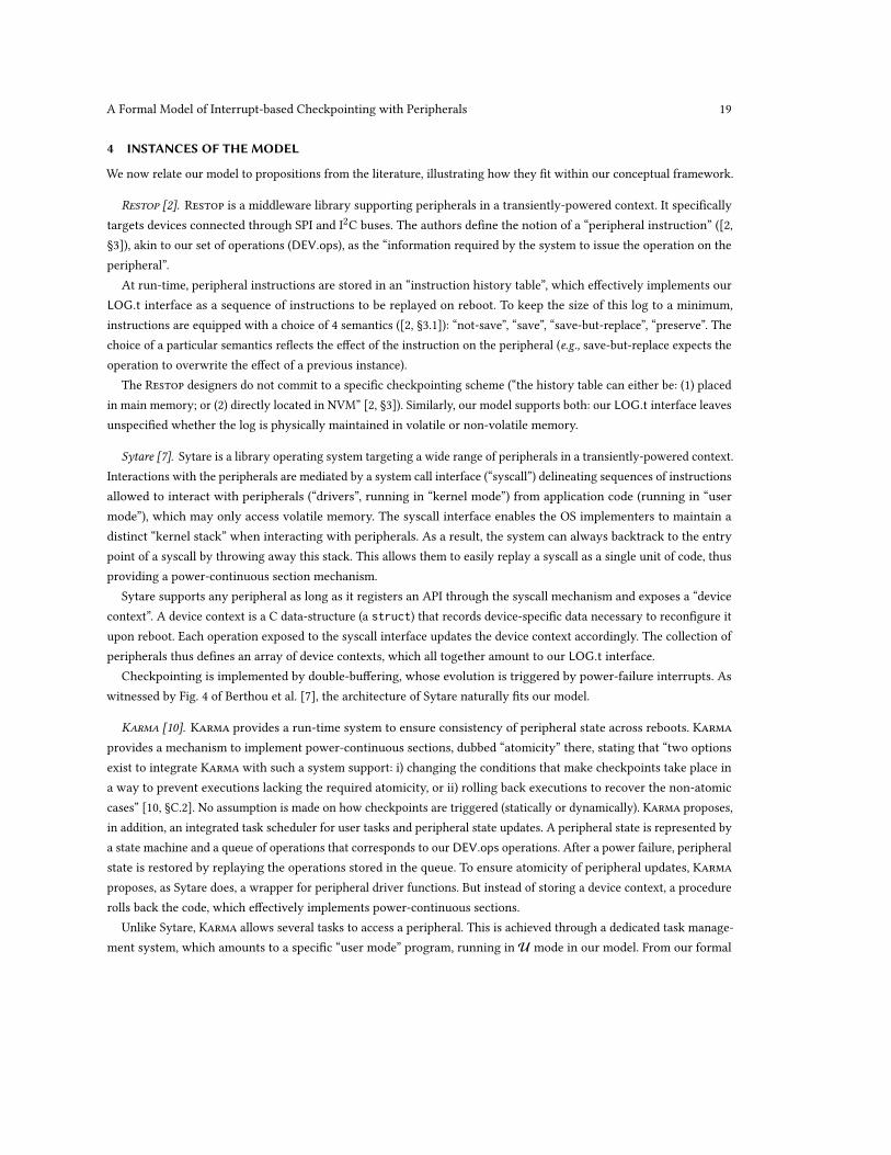
Restop [2]. Restop is a middleware library supporting peripherals in a transiently-powered context. It specifically

targets devices connected through SPI and I2C buses. The authors define the notion of a “peripheral instruction” ([2,

§3]), akin to our set of operations (DEV.ops), as the “information required by the system to issue the operation on the

peripheral”.

At run-time, peripheral instructions are stored in an “instruction history table”, which effectively implements our

LOG.t interface as a sequence of instructions to be replayed on reboot. To keep the size of this log to a minimum,

instructions are equipped with a choice of 4 semantics ([2, §3.1]): “not-save”, “save”, “save-but-replace”, “preserve”. The

choice of a particular semantics reflects the effect of the instruction on the peripheral (e.g., save-but-replace expects the

operation to overwrite the effect of a previous instance).

The Restop designers do not commit to a specific checkpointing scheme (“the history table can either be: (1) placed

in main memory; or (2) directly located in NVM” [2, §3]). Similarly, our model supports both: our LOG.t interface leaves

unspecified whether the log is physically maintained in volatile or non-volatile memory.

Sytare [7]. Sytare is a library operating system targeting a wide range of peripherals in a transiently-powered context.

Interactions with the peripherals are mediated by a system call interface (“syscall”) delineating sequences of instructions

allowed to interact with peripherals (“drivers”, running in “kernel mode”) from application code (running in “user

mode”), which may only access volatile memory. The syscall interface enables the OS implementers to maintain a

distinct “kernel stack” when interacting with peripherals. As a result, the system can always backtrack to the entry

point of a syscall by throwing away this stack. This allows them to easily replay a syscall as a single unit of code, thus

providing a power-continuous section mechanism.

Sytare supports any peripheral as long as it registers an API through the syscall mechanism and exposes a “device

context”. A device context is a C data-structure (a struct) that records device-specific data necessary to reconfigure it

upon reboot. Each operation exposed to the syscall interface updates the device context accordingly. The collection of

peripherals thus defines an array of device contexts, which all together amount to our LOG.t interface.

Checkpointing is implemented by double-buffering, whose evolution is triggered by power-failure interrupts. As

witnessed by Fig. 4 of Berthou et al. [7], the architecture of Sytare naturally fits our model.

Karma [10]. Karma provides a run-time system to ensure consistency of peripheral state across reboots. Karma

provides a mechanism to implement power-continuous sections, dubbed “atomicity” there, stating that “two options

exist to integrate Karma with such a system support: i) changing the conditions that make checkpoints take place in

a way to prevent executions lacking the required atomicity, or ii) rolling back executions to recover the non-atomic

cases” [10, §C.2]. No assumption is made on how checkpoints are triggered (statically or dynamically). Karma proposes,

in addition, an integrated task scheduler for user tasks and peripheral state updates. A peripheral state is represented by

a state machine and a queue of operations that corresponds to our DEV.ops operations. After a power failure, peripheral

state is restored by replaying the operations stored in the queue. To ensure atomicity of peripheral updates, Karma

proposes, as Sytare does, a wrapper for peripheral driver functions. But instead of storing a device context, a procedure

rolls back the code, which effectively implements power-continuous sections.

Unlike Sytare, Karma allows several tasks to access a peripheral. This is achieved through a dedicated task manage-

ment system, which amounts to a specific “user mode” program, running inU mode in our model. From our formal

20 Gautier Berthou, Pierre-Évariste Dagand, Delphine Demange, Rémi Oudin, and Tanguy Risset

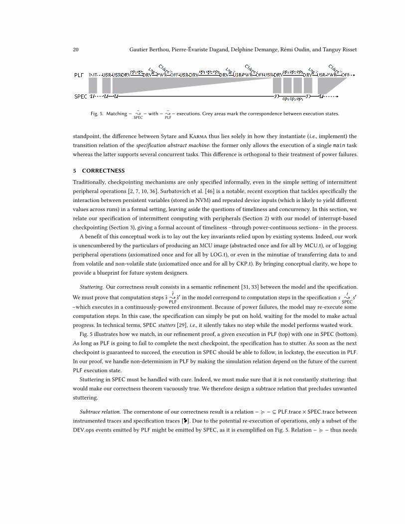
Fig. 5. Matching − −{SPEC

− with − −{PLF

− executions. Grey areas mark the correspondence between execution states.

standpoint, the difference between Sytare and Karma thus lies solely in how they instantiate (i.e., implement) the

transition relation of the specification abstract machine: the former only allows the execution of a single main task

whereas the latter supports several concurrent tasks. This difference is orthogonal to their treatment of power failures.

5 CORRECTNESS

Traditionally, checkpointing mechanisms are only specified informally, even in the simple setting of intermittent

peripheral operations [2, 7, 10, 36]. Surbatovich et al. [46] is a notable, recent exception that tackles specifically the

interaction between persistent variables (stored in NVM) and repeated device inputs (which is likely to yield different

values across runs) in a formal setting, leaving aside the questions of timeliness and concurrency. In this section, we

relate our specification of intermittent computing with peripherals (Section 2) with our model of interrupt-based

checkpointing (Section 3), giving a formal account of timeliness –through power-continuous sections– in the process.

A benefit of this conceptual work is to lay out the key invariants relied upon by existing systems. Indeed, our work

is unencumbered by the particulars of producing an MCU image (abstracted once and for all byMCU.t), or of logging

peripheral operations (axiomatized once and for all by LOG.t), or even in the minutiae of transferring data to and

from volatile and non-volatile state (axiomatized once and for all by CKP.t). By bringing conceptual clarity, we hope to

provide a blueprint for future system designers.

Stuttering. Our correctness result consists in a semantic refinement [31, 33] between the model and the specification.

We must prove that computation steps s

t

{PLF

s′in the model correspond to computation steps in the specification s

t

{SPEC

s′

–which executes in a continuously-powered environment. Because of power failures, the model may re-execute some

computation steps. In this case, the specification can simply be put on hold, waiting for the model to make actual

progress. In technical terms, SPEC stutters [29], i.e., it silently takes no step while the model performs wasted work.

Fig. 5 illustrates how we match, in our refinement proof, a given execution in PLF (top) with one in SPEC (bottom).

As long as PLF is going to fail to complete the next checkpoint, the specification has to stutter. As soon as the next

checkpoint is guaranteed to succeed, the execution in SPEC should be able to follow, in lockstep, the execution in PLF.

In our proof, we handle non-determinism in PLF by making the simulation relation depend on the future of the current

PLF execution state.

Stuttering in SPEC must be handled with care. Indeed, we must make sure that it is not constantly stuttering: that

would make our correctness theorem vacuously true. We therefore design a subtrace relation that precludes unwanted

stuttering.

Subtrace relation. The cornerstone of our correctness result is a relation − ≽ − ⊆ PLF.trace × SPEC.trace between

instrumented traces and specification traces [ ]. Due to the potential re-execution of operations, only a subset of the

DEV.ops events emitted by PLF might be emitted by SPEC, as it is exemplified on Fig. 5. Relation − ≽ − thus needs

A Formal Model of Interrupt-based Checkpointing with Peripherals 21

to enforce a subtrace relation. Besides, we want to ensure that power-continuous sections –sequences of operations

delineated by Enter/Leave– are eventually executed within a single run.

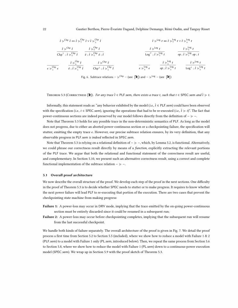
Intuitively, given a trace 𝑡 ∈ PLF.trace, we first filter all subtraces where the checkpointing succeeds, leading a trace

containing events in {Log⊤, Log⊥} ⊎ DEV.ops, conventionally written as 𝑡 . We write 𝑒 for any such observable event.

Then, within each of these subtraces, we select the events of power-continuous sections that completed without a power

failure, thereby obtaining a trace 𝑡 ∈ SPEC.trace. We hence define the subtrace relation − ≽ − as a composition of two

subtrace relations (defined in Fig. 6):

Definition 5.1 (Subtrace relation ≽ [ ]). Let t ∈ PLF.trace and t ∈ SPEC.trace. By definition, we have t ≽ t if and

only if there exists t ∈ ({Log⊤, Log⊥} ⊎ DEV.ops)∗, such that t ≽Ckpt ∧ t ≽Log

t.

Relation − ≽Ckp − deals with re-execution of code upon a checkpointing failure (transition Ckp-Fail), filtering out

sub-sequences of events that end with Ckp⊥, while retaining any other event leading to a Ckp⊤. Similarly, relation

− ≽Log − deals with re-execution of code upon a power-failure interrupt in driver mode (transition DrvPwr), filtering

out sub-sequences of operations ending with a Log⊥, while retaining the remaining operations.

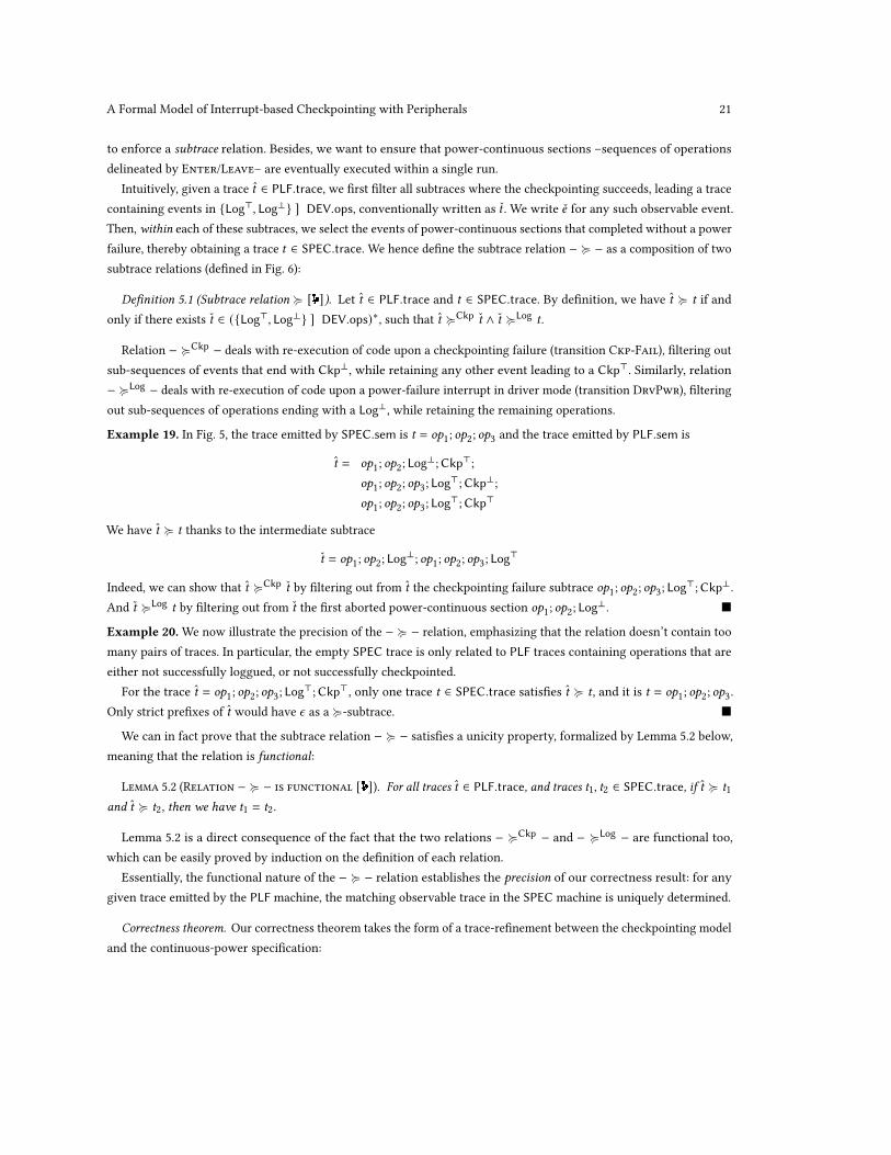
Example 19. In Fig. 5, the trace emitted by SPEC.sem is t = op1; op

2; op

3and the trace emitted by PLF.sem is

t = op1; op

2; Log⊥;Ckp⊤;

op1; op

2; op

3; Log⊤;Ckp⊥;

op1; op

2; op

3; Log⊤;Ckp⊤

We have t ≽ t thanks to the intermediate subtrace

t = op1; op

2; Log⊥; op

1; op

2; op

3; Log⊤

Indeed, we can show that t ≽Ckpt by filtering out from t the checkpointing failure subtrace op

1; op

2; op

3; Log⊤;Ckp⊥.

And t ≽Logt by filtering out from t the first aborted power-continuous section op

1; op

2; Log⊥. ■

Example 20. We now illustrate the precision of the − ≽ − relation, emphasizing that the relation doesn’t contain too

many pairs of traces. In particular, the empty SPEC trace is only related to PLF traces containing operations that are

either not successfully loggued, or not successfully checkpointed.

For the trace t = op1; op

2; op

3; Log⊤;Ckp⊤, only one trace t ∈ SPEC.trace satisfies t ≽ t, and it is t = op

1; op

2; op

3.

Only strict prefixes of t would have 𝜖 as a ≽-subtrace. ■

We can in fact prove that the subtrace relation − ≽ − satisfies a unicity property, formalized by Lemma 5.2 below,

meaning that the relation is functional:

Lemma 5.2 (Relation − ≽ − is functional [ ]). For all traces t ∈ PLF.trace, and traces t1, t2 ∈ SPEC.trace, if t ≽ t1

and t ≽ t2, then we have t1 = t2.

Lemma 5.2 is a direct consequence of the fact that the two relations − ≽Ckp − and − ≽Log − are functional too,

which can be easily proved by induction on the definition of each relation.

Essentially, the functional nature of the − ≽ − relation establishes the precision of our correctness result: for any

given trace emitted by the PLF machine, the matching observable trace in the SPEC machine is uniquely determined.

Correctness theorem. Our correctness theorem takes the form of a trace-refinement between the checkpointing model

and the continuous-power specification:

22 Gautier Berthou, Pierre-Évariste Dagand, Delphine Demange, Rémi Oudin, and Tanguy Risset

𝑡 ≽Ckp 𝑡 ⇔ 𝑡 ≽Ckp⊤ 𝑡 ∨ 𝑡 ≽Ckp

⊥ 𝑡

𝑡 ≽Ckp 𝑡

Ckp⊤ ; 𝑡 ≽Ckp⊤ 𝑡

𝑡 ≽Ckp⊤ 𝑡

𝑒 ; 𝑡 ≽Ckp⊤ 𝑒 ; 𝑡

𝜖 ≽Ckp⊥ 𝜖

𝑡 ≽Ckp⊥ 𝑡

𝑒 ; 𝑡 ≽Ckp⊥ 𝑡

𝑡 ≽Ckp 𝑡

Ckp⊥ ; 𝑡 ≽Ckp⊥ 𝑡

𝑡 ≽Log 𝑡 ⇔ 𝑡 ≽Log⊤ 𝑡 ∨ 𝑡 ≽Log

⊥ 𝑡

𝑡 ≽Log 𝑡

Log⊤ ; 𝑡 ≽Log⊤ 𝑡

𝑡 ≽Log⊤ 𝑡

op ; 𝑡 ≽Log⊤ op ; 𝑡

𝜖 ≽Log⊥ 𝜖

𝑡 ≽Log⊥ 𝑡

op ; 𝑡 ≽Log⊥ 𝑡

𝑡 ≽Log 𝑡

Log⊥ ; 𝑡 ≽Log⊥ 𝑡

Fig. 6. Subtrace relations − ≽Ckp − (see[ ]

) and − ≽Log − (see[ ]

)

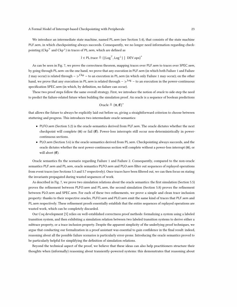
Theorem 5.3 (Correctness [ ]). For any trace t ∈ PLF.sem, there exists a trace t, such that t ∈ SPEC.sem and t ≽ t.

Informally, this statement reads as: “any behavior exhibited by the model (i.e., t ∈ PLF.sem) could have been observed

with the specification (i.e., t ∈ SPEC.sem), ignoring the operations that had to be re-executed (i.e., t ≽ t)”. The fact that

power-continuous sections are indeed preserved by our model follows directly from the definition of − ≽ −.Note that Theorem 5.3 holds for any possible trace in the non-deterministic semantics of PLF. As long as the model

does not progress, due to either an aborted power-continuous section or a checkpointing failure, the specification will

stutter, emitting the empty trace 𝜖 . However, our precise subtrace relation ensures, by its very definition, that any

observable progress in PLF.sem is indeed reflected in SPEC.sem.

Note that Theorem 5.3 is relying on a relational definition of − ≽ −, which, by Lemma 5.2, is functional. Alternatively,

we could phrase our correctness result directly by means of a function, explicitly extracting the relevant portions

of the PLF trace. We argue that both the relational and functional statement of the correctness result are useful,

and complementary. In Section 5.10, we present such an alternative correctness result, using a correct and complete

functional implementation of the subtrace relation − ≽ −.

5.1 Overall proof architecture

We now describe the overall structure of the proof. We develop each step of the proof in the next sections. One difficulty

in the proof of Theorem 5.3 is to decide whether SPEC needs to stutter or to make progress. It requires to know whether

the next power failure will lead PLF to re-executing that portion of the execution. There are two cases that prevent the

checkpointing state machine from making progress:

Failure 1: A power-loss may occur in DRV mode, implying that the trace emitted by the on-going power-continuous

section must be entirely discarded since it could be resumed in a subsequent run;

Failure 2: A power-loss may occur before checkpointing completes, implying that the subsequent run will resume

from the last successful checkpoint.

We handle both kinds of failure separately. The overall architecture of the proof is given in Fig. 7. We detail the proof

process a first time from Section 5.2 to Section 5.5 (included), where we show how to reduce a model with Failure 1 & 2

(PLF.sem) to a model with Failure 1 only (PL.sem, introduced below). Then, we repeat the same process from Section 5.6

to Section 5.8, where we show how to reduce the model with Failure 1 (PL.sem) down to a continuous-power execution

model (SPEC.sem). We wrap up in Section 5.9 with the proof sketch of Theorem 5.3.

A Formal Model of Interrupt-based Checkpointing with Peripherals 23

We introduce an intermediate state machine, named PL.sem (see Section 5.4), that consists of the state machine

PLF.sem, in which checkpointing always succeeds. Consequently, we no longer need information regarding check-

pointing (Ckp⊤ and Ckp⊥) in traces of PL.sem, which are defined as

t ∈ PL.trace ≜({Log⊤, Log⊥} ⊎ DEV.ops

)∗As can be seen in Fig. 7, we prove the correctness theorem, mapping traces over PLF.sem to traces over SPEC.sem,

by going through PL.sem: on the one hand, we prove that any execution in PLF.sem (in which both Failure 1 and Failure

2 may occur) is related through − ≽Ckp − to an execution in PL.sem (in which only Failure 1 may occur); on the other

hand, we prove that any execution in PL.sem is related through − ≽Log − to an execution in the power-continuous

specification SPEC.sem (in which, by definition, no failure can occur).

These two proof steps follow the same overall strategy. First, we introduce the notion of oracle to side-step the need

to predict the failure-related future when building the simulation proof. An oracle is a sequence of boolean predictions

Oracle ≜ {tt,ff}∗

that allows the future to always be explicitly laid out before us, giving a straightforward criterion to choose between

stuttering and progress. This introduces two intermediate oracle-semantics:

• PLFO.sem (Section 5.2) is the oracle-semantics derived from PLF.sem. The oracle dictates whether the next

checkpoint will complete (tt) or fail (ff). Power-loss interrupts still occur non-deterministically in power-

continuous sections.

• PLO.sem (Section 5.6) is the oracle-semantics derived from PL.sem. Checkpointing always succeeds, and the

oracle dictates whether the next power-continuous section will complete without a power-loss interrupt (tt), orwill abort (ff).

Oracle semantics fix the scenario regarding Failure 1 and Failure 2. Consequently, compared to the non-oracle

semantics PLF.sem and PL.sem, oracle semantics PLFO.sem and PLO.sem filter out sequences of replayed operations

from event traces (see Sections 5.3 and 5.7 respectively). Once traces have been filtered out, we can then focus on stating

the invariants propagated during wasted sequences of work.

As described in Fig. 7, we prove two simulation relations about the oracle semantics: the first simulation (Section 5.5)

proves the refinement between PLFO.sem and PL.sem, the second simulation (Section 5.8) proves the refinement

between PLO.sem and SPEC.sem. For each of these two refinements, we prove a simple and clean trace inclusion

property: thanks to their respective oracles, PLFO.sem and PLO.sem emit the same kind of traces that PLF.sem and

PL.sem respectively. These refinement proofs essentially establish that the entire sequences of replayed operations are

wasted work, which can be completely discarded.

Our Coq development [5] relies on well-established correctness proof methods: formalizing a system using a labeled

transition system, and then exhibiting a simulation relation between two labeled transition systems to derive either a

subtrace property, or a trace inclusion property. Despite the apparent simplicity of the underlying proof techniques, we

argue that conducting our formalization in a proof assistant was essential to gain confidence in the final result: indeed,

reasoning about all the possible failure scenarios is particularly error-prone. Introducing the oracle semantics proved to

be particularly helpful for simplifying the definition of simulation relations.

Beyond the technical aspect of the proof, we believe that these ideas can also help practitioners structure their

thoughts when (informally) reasoning about transiently-powered systems: this demonstrates that reasoning about

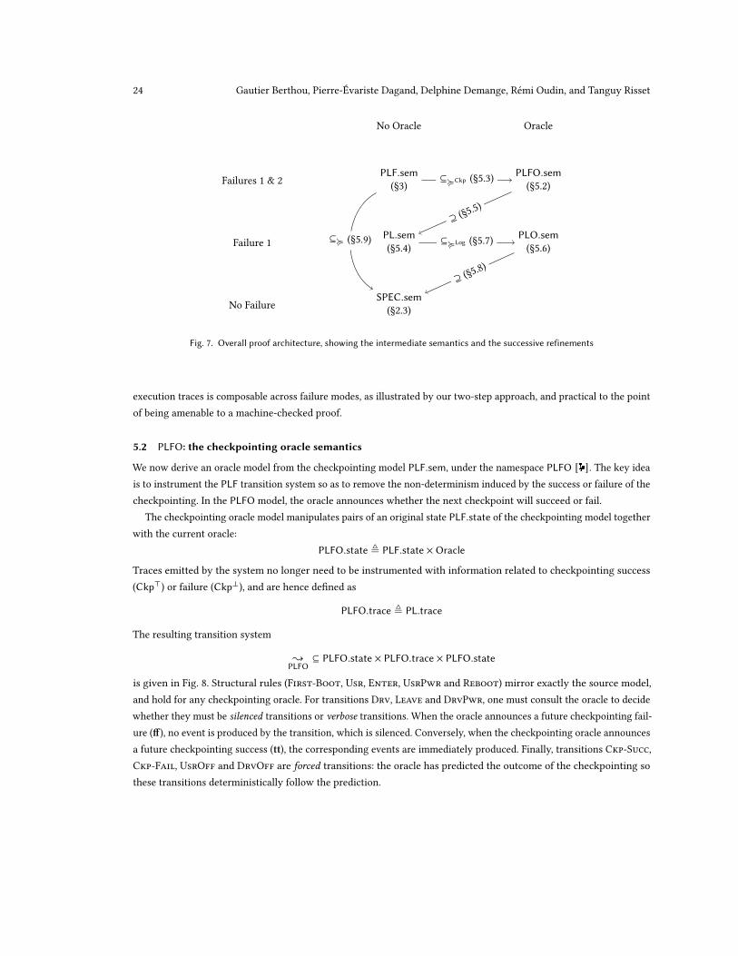
24 Gautier Berthou, Pierre-Évariste Dagand, Delphine Demange, Rémi Oudin, and Tanguy Risset

No Oracle Oracle

Failures 1 & 2

PLF.sem(§3)

PLFO.sem(§5.2)

Failure 1

PL.sem(§5.4)

PLO.sem(§5.6)

No Failure

SPEC.sem(§2.3)

⊇ (§5.8)

⊆≽Log (§5.7)

⊇ (§5.5)

⊆≽Ckp (§5.3)

⊆≽ (§5.9)

Fig. 7. Overall proof architecture, showing the intermediate semantics and the successive refinements

execution traces is composable across failure modes, as illustrated by our two-step approach, and practical to the point

of being amenable to a machine-checked proof.

5.2 PLFO: the checkpointing oracle semantics

We now derive an oracle model from the checkpointing model PLF.sem, under the namespace PLFO [ ]. The key idea

is to instrument the PLF transition system so as to remove the non-determinism induced by the success or failure of the

checkpointing. In the PLFO model, the oracle announces whether the next checkpoint will succeed or fail.

The checkpointing oracle model manipulates pairs of an original state PLF.state of the checkpointing model together

with the current oracle:

PLFO.state ≜ PLF.state ×Oracle

Traces emitted by the system no longer need to be instrumented with information related to checkpointing success

(Ckp⊤) or failure (Ckp⊥), and are hence defined as

PLFO.trace ≜ PL.trace

The resulting transition system

{PLFO

⊆ PLFO.state × PLFO.trace × PLFO.state

is given in Fig. 8. Structural rules (First-Boot, Usr, Enter, UsrPwr and Reboot) mirror exactly the source model,

and hold for any checkpointing oracle. For transitions Drv, Leave and DrvPwr, one must consult the oracle to decide

whether they must be silenced transitions or verbose transitions. When the oracle announces a future checkpointing fail-

ure (ff), no event is produced by the transition, which is silenced. Conversely, when the checkpointing oracle announces

a future checkpointing success (tt), the corresponding events are immediately produced. Finally, transitions Ckp-Succ,

Ckp-Fail, UsrOff and DrvOff are forced transitions: the oracle has predicted the outcome of the checkpointing so

these transitions deterministically follow the prediction.

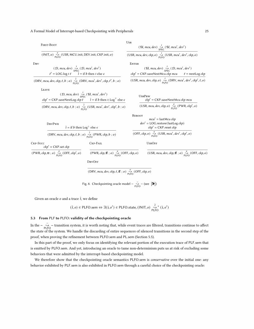
A Formal Model of Interrupt-based Checkpointing with Peripherals 25

First-Boot

(INIT, 𝑜 ) 𝜖{

PLFO(USR,MCU.init,DEV.init,CKP.init, 𝑜 )

Usr

(U,mcu, dev) t

{SPEC

(U,mcu′, dev′ )

(USR,mcu, dev, ckp, 𝑜 ) t

{PLFO

(USR,mcu′, dev′, ckp, 𝑜 )

Drv

(D,mcu, dev) t

{SPEC

(D,mcu′, dev′ )

ℓ ′ = LOG.log t ℓ t = if 𝑏 then t else 𝜖

(DRV,mcu, dev, ckp, ℓ, 𝑏 ; 𝑜 ) t

{PLFO

(DRV,mcu′, dev′, ckp, ℓ ′, 𝑏 ; 𝑜 )

Enter

(U,mcu, dev) t

{SPEC

(D,mcu′, dev′ )

ckp′ = CKP.saveNextMcu ckp mcu ℓ = nextLog ckp

(USR,mcu, dev, ckp, 𝑜 ) t

{PLFO

(DRV,mcu′, dev′, ckp′, ℓ, 𝑜 )

Leave

(D,mcu, dev) t

{SPEC

(U,mcu′, dev′ )

ckp′ = CKP.saveNextLog ckp ℓ t = if 𝑏 then t; Log⊤ else 𝜖

(DRV,mcu, dev, ckp, ℓ, 𝑏 ; 𝑜 ) t

{PLFO

(USR,mcu′, dev′, ckp′, 𝑏 ; 𝑜 )

UsrPrw

ckp′ = CKP.saveNextMcu ckp mcu

(USR,mcu, dev, ckp, 𝑜 ) 𝜖{

PLFO(PWR, ckp′, 𝑜 )

DrvPwr

t = if 𝑏 then Log⊥ else 𝜖

(DRV,mcu, dev, ckp, ℓ, 𝑏 ; 𝑜 ) t

{PLFO

(PWR, ckp, 𝑏 ; 𝑜 )

Reboot

mcu′ = lastMcu ckp

dev′ = LOG.restore(lastLog ckp)

ckp′ = CKP.reset ckp

(OFF, ckp, 𝑜 ) 𝜖{

PLFO(USR,mcu

′, dev′, ckp′, 𝑜 )

Ckp-Succ

ckp′ = CKP.set ckp

(PWR, ckp, tt ; 𝑜 ) 𝜖{

PLFO(OFF, ckp′, 𝑜 )

Ckp-Fail

(PWR, ckp,ff ; 𝑜 ) 𝜖{

PLFO(OFF, ckp, 𝑜 )

UsrOff

(USR,mcu, dev, ckp,ff ; 𝑜 ) 𝜖{

PLFO(OFF, ckp, 𝑜 )

DrvOff

(DRV,mcu, dev, ckp, ℓ,ff ; 𝑜 ) 𝜖{

PLFO(OFF, ckp, 𝑜 )

Fig. 8. Checkpointing oracle model − −{

PLFO− (see

[ ])

Given an oracle 𝑜 and a trace t, we define

(t, 𝑜) ∈ PLFO.sem ⇔ ∃(s, 𝑜′) ∈ PLFO.state, (INIT, 𝑜) t

{PLFO

∗ (s, 𝑜′)

5.3 From PLF to PLFO: validity of the checkpointing oracle

In the − −{

PLFO− transition system, it is worth noting that, while event traces are filtered, transitions continue to affect

the state of the system. We handle the discarding of entire sequences of silenced transitions in the second step of the

proof, when proving the refinement between PLFO.sem and PL.sem (Section 5.5).

In this part of the proof, we only focus on identifying the relevant portion of the execution trace of PLF.sem that

is emitted by PLFO.sem. And yet, introducing an oracle to tame non-determinism puts us at risk of excluding some

behaviors that were admitted by the interrupt-based checkpointing model.

We therefore show that the checkpointing oracle semantics PLFO.sem is conservative over the initial one: any

behavior exhibited by PLF.sem is also exhibited in PLFO.sem through a careful choice of the checkpointing oracle:

26 Gautier Berthou, Pierre-Évariste Dagand, Delphine Demange, Rémi Oudin, and Tanguy Risset

Fig. 9. Matching executions across the whole refinement chain

Lemma 5.4 (Validity of the checkpointing oracle [ ]). For any trace t ∈ PLF.trace such that t ∈ PLF.sem, there

exists an oracle 𝑜 and a trace t such that (t, 𝑜) ∈ PLFO.sem, satisfying t ≽Ckpt.

In Coq, the proof calls for effectively building an oracle for any possible trace, as we have to inhabit the existential

witness in the conclusion. To this end, we rely on a definition of trace that provides a useful induction principle:

the reflexive-transitive closure of the stepping relation − −{PLF

− is defined as right-recursive. This way, the induction

hypothesis gives us an oracle that we have to complete from right to left. The last step performed in − −{PLF

− guides us

to choose between (1) prepending to the current oracle the decision that corresponds to the emission of either a Ckp⊥

or a Ckp⊤ event or (2) keeping the same, current oracle for any other kind of transition.

Let us illustrate Lemma 5.4 with Figure 9. The PLF.sem trace (top) is the same as in Figure 5. Just below, we represent

the corresponding execution sequence in PLFO.sem that we prove to satisfy the − ≽Ckp − relation. The execution

sequence is represented with a two-level timeline, indicating whether the checkpointing oracle is predicting a future

successful checkpoint (higher level) or a future failing checkpoint (lower level). The central portion of the execution

trace is the portion that will be replayed because of checkpointing failure. Hence, the oracle is chosen accordingly, and

the corresponding transitions are silenced.

5.4 PL: checkpointing model without checkpointing failures

Our intermediate model, defined under the namespace PL [ ] is derived from the PLFmodel, by removing the possibility

for checkpointing to fail, while keeping the possibility of aborting power-continuous sections with a power-loss interrupt.

The PL transition system is defined over traces

t ∈ PL.trace ≜ ({Log⊤, Log⊥} ⊎ DEV.ops)∗

As previously explained, checkpointing events (both Ckp⊤ and Ckp⊥) cannot occur, since checkpointing always

succeeds.

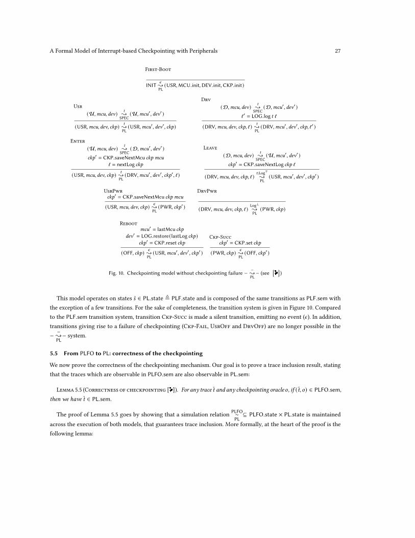
A Formal Model of Interrupt-based Checkpointing with Peripherals 27

First-Boot

INIT𝜖{PL

(USR,MCU.init,DEV.init,CKP.init)

Usr

(U,mcu, dev) t

{SPEC

(U,mcu′, dev′ )

(USR,mcu, dev, ckp) t

{PL

(USR,mcu′, dev′, ckp)

Drv

(D,mcu, dev) t

{SPEC

(D,mcu′, dev′ )

ℓ ′ = LOG.log t ℓ

(DRV,mcu, dev, ckp, ℓ ) t

{PL

(DRV,mcu′, dev′, ckp, ℓ ′ )

Enter

(U,mcu, dev) t

{SPEC

(D,mcu′, dev′ )

ckp′ = CKP.saveNextMcu ckp mcu

ℓ = nextLog ckp

(USR,mcu, dev, ckp) t

{PL

(DRV,mcu′, dev′, ckp′, ℓ )

Leave

(D,mcu, dev) t

{SPEC

(U,mcu′, dev′ )

ckp′ = CKP.saveNextLog ckp ℓ

(DRV,mcu, dev, ckp, ℓ )t;Log⊤{PL

(USR,mcu′, dev′, ckp′ )

UsrPwr

ckp′ = CKP.saveNextMcu ckp mcu

(USR,mcu, dev, ckp) 𝜖{PL

(PWR, ckp′ )

DrvPwr

(DRV,mcu, dev, ckp, ℓ )Log⊥{PL

(PWR, ckp)

Reboot

mcu′ = lastMcu ckp

dev′ = LOG.restore(lastLog ckp)

ckp′ = CKP.reset ckp

(OFF, ckp) 𝜖{PL

(USR,mcu′, dev′, ckp′ )

Ckp-Succ

ckp′ = CKP.set ckp

(PWR, ckp) 𝜖{PL

(OFF, ckp′ )

Fig. 10. Checkpointing model without checkpointing failure − −{PL

− (see[ ]

)

This model operates on states 𝑠 ∈ PL.state ≜ PLF.state and is composed of the same transitions as PLF.sem with

the exception of a few transitions. For the sake of completeness, the transition system is given in Figure 10. Compared

to the PLF.sem transition system, transition Ckp-Succ is made a silent transition, emitting no event (𝜖). In addition,

transitions giving rise to a failure of checkpointing (Ckp-Fail, UsrOff and DrvOff) are no longer possible in the

− −{PL

− system.

5.5 From PLFO to PL: correctness of the checkpointing

We now prove the correctness of the checkpointing mechanism. Our goal is to prove a trace inclusion result, stating

that the traces which are observable in PLFO.sem are also observable in PL.sem:

Lemma 5.5 (Correctness of checkpointing [ ]). For any trace t and any checkpointing oracle 𝑜 , if (t, 𝑜) ∈ PLFO.sem,

then we have t ∈ PL.sem.

The proof of Lemma 5.5 goes by showing that a simulation relationPLFO∼PL

⊆ PLFO.state × PL.state is maintained

across the execution of both models, that guarantees trace inclusion. More formally, at the heart of the proof is the

following lemma:

28 Gautier Berthou, Pierre-Évariste Dagand, Delphine Demange, Rémi Oudin, and Tanguy Risset

Lemma 5.6 (Star-simulation diagram between PLFO and PL transition systems [ ]). For all (s1, 𝑜1), (s2, 𝑜2) ∈PLFO.state, and any trace t, if (s1, 𝑜1)

t

{PLFO

(s2, 𝑜2), then for all states 𝑠1, such that (s1, 𝑜1) PLFO∼PL

𝑠1, then there exists a

state 𝑠2 such that 𝑠1

t

{PL∗ 𝑠2 and (s2, 𝑜2) PLFO∼

PL𝑠2.

Correctly handling the stuttering of PL.sem is key here: some transitions in PLFO.sem will eventually be aborted, so

we must keep PL.sem from taking a transition forward. To solve this issue, we rely on the checkpointing oracle whose

purpose is precisely to tell whether the next checkpointing will success or not.

Intuitively, the idea is to let PL.sem stutter in an OFF state as long as the next checkpointing will fail. Conversely,

when the checkpointing oracle predicts that the next checkpointing will succeed, the two transition systems will

proceed in lock-step. This is illustrated in Figure 9: the checkpointing oracle for the example PLFO.sem execution

is tt ; ff ; tt ; (. . .). Before the first power-loss of PLFO.sem, transitions are performed in a lockstep fashion in both

machines, because the checkpointing oracle predicts the success of the next checkpointing. At that point, the PL.sem

machine steps in a reboot state, in which it will stutter for the next transition steps done in PLFO.sem, up until the

point where the PLFO.sem machine restarts in a state where the oracle is predicting that the future checkpointing will

succeed.

Letting PL.sem stutter in a reboot state while PLFO.sem is making some (silenced) computation steps raises the

following concern: at the point where PL.sem starts again to step, we ought to prove that the two machines can indeed

proceed back in lock-step. For this to hold, both machines should agree on their non-volatile checkpointing storage.

But, each time the PL.sem machine is reaching an OFF state, the checkpointing it just performed was successful

(CKP.set), hence both of its last and next snapshots are consistent. In contrast, when the PLFO.sem steps while the

oracle predicts a future failure, it keeps updating its next snapshot.

The crux of the simulation proof is an invariant stating that, during the whole subsequence of steps where the oracle

is predicting the failure of the next checkpoint, both systems continue to agree on their last snapshots. Indeed, only the

next snapshot is updated during the silenced computation steps of PLFO.sem, the last snapshot is kept untouched, and

the checkpointing storage is CKP.reset at reboots.

The simulation relation − PLFO∼PL

− we define embeds these invariants, plus some additional technicalities. It is defined

in Figure 11, where the function ckp ∈ PLF.state → CKP.t extracts the non-volatile checkpointing storage of a state.

Initial states match for any oracle (rule Init). Rules Step and StepOff apply when both machines execute in lock-step,

when the oracle predicts a future successful checkpointing (tt), until they reach anOFF state. Conversely, rules Stutter

and StutterOff apply when the PL.sem machine stutters, again until they reach an OFF state. The last two rules

StutterInit and StutterInitOff correspond to the situation where the PL.sem machine has to stutter in its initial

states. This is the case when the PLFO.sem machine executes while no previous successful checkpointing was ever

made. In this rules, we only need to maintain the invariant that the last snapshots of both machines are consistent. The

fact that the last and next snapshots of the PL.sem machine are in sync is obtained by the definition of CKP.init.

5.6 PLO: the logging oracle semantics

The next step of the proof is to establish a correspondence between PL.sem and SPEC.sem. We apply the same

methodology as previously, which consists in defining an intermediate oracle-semantics PLO.sem, derived from PL.sem.

The system will operate on states

PLO.state ≜ PL.state ×Oracle

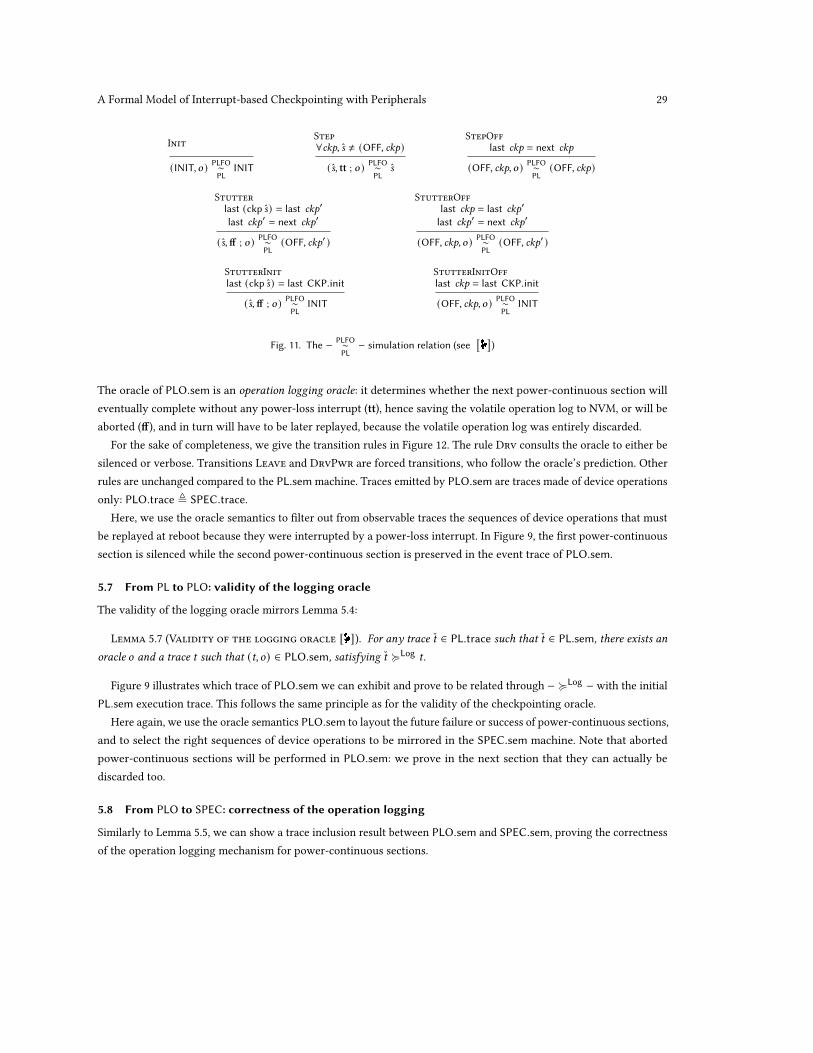
A Formal Model of Interrupt-based Checkpointing with Peripherals 29

Init

(INIT, 𝑜 ) PLFO∼PL

INIT

Step

∀ckp, s ≠ (OFF, ckp)

(s, tt ; 𝑜 ) PLFO∼PL

s

StepOff

last ckp = next ckp

(OFF, ckp, 𝑜 ) PLFO∼PL

(OFF, ckp)

Stutter

last (ckp s) = last ckp′

last ckp′ = next ckp′

(s,ff ; 𝑜 ) PLFO∼PL

(OFF, ckp′ )

StutterOff

last ckp = last ckp′

last ckp′ = next ckp′

(OFF, ckp, 𝑜 ) PLFO∼PL

(OFF, ckp′ )

StutterInit

last (ckp s) = last CKP.init

(s,ff ; 𝑜 ) PLFO∼PL

INIT

StutterInitOff

last ckp = last CKP.init

(OFF, ckp, 𝑜 ) PLFO∼PL

INIT

Fig. 11. The − PLFO∼PL

− simulation relation (see[ ]

)

The oracle of PLO.sem is an operation logging oracle: it determines whether the next power-continuous section will

eventually complete without any power-loss interrupt (tt), hence saving the volatile operation log to NVM, or will be

aborted (ff), and in turn will have to be later replayed, because the volatile operation log was entirely discarded.

For the sake of completeness, we give the transition rules in Figure 12. The rule Drv consults the oracle to either be

silenced or verbose. Transitions Leave and DrvPwr are forced transitions, who follow the oracle’s prediction. Other

rules are unchanged compared to the PL.semmachine. Traces emitted by PLO.sem are traces made of device operations

only: PLO.trace ≜ SPEC.trace.

Here, we use the oracle semantics to filter out from observable traces the sequences of device operations that must

be replayed at reboot because they were interrupted by a power-loss interrupt. In Figure 9, the first power-continuous

section is silenced while the second power-continuous section is preserved in the event trace of PLO.sem.

5.7 From PL to PLO: validity of the logging oracle

The validity of the logging oracle mirrors Lemma 5.4:

Lemma 5.7 (Validity of the logging oracle [ ]). For any trace t ∈ PL.trace such that t ∈ PL.sem, there exists an

oracle 𝑜 and a trace t such that (t, 𝑜) ∈ PLO.sem, satisfying t ≽Logt.

Figure 9 illustrates which trace of PLO.sem we can exhibit and prove to be related through − ≽Log − with the initial

PL.sem execution trace. This follows the same principle as for the validity of the checkpointing oracle.

Here again, we use the oracle semantics PLO.sem to layout the future failure or success of power-continuous sections,

and to select the right sequences of device operations to be mirrored in the SPEC.sem machine. Note that aborted

power-continuous sections will be performed in PLO.sem: we prove in the next section that they can actually be

discarded too.

5.8 From PLO to SPEC: correctness of the operation logging

Similarly to Lemma 5.5, we can show a trace inclusion result between PLO.sem and SPEC.sem, proving the correctness

of the operation logging mechanism for power-continuous sections.

30 Gautier Berthou, Pierre-Évariste Dagand, Delphine Demange, Rémi Oudin, and Tanguy Risset

First-Boot

(INIT, 𝑜 ) 𝜖{PLO

(USR,MCU.init,DEV.init,CKP.init, 𝑜 )

Usr

(U,mcu, dev) t

{SPEC

(U,mcu′, dev′ )

(USR,mcu, dev, ckp, 𝑜 ) t

{PLO

(USR,mcu′, dev′, ckp, 𝑜 )

Drv

(D,mcu, dev) t

{SPEC

(D,mcu′, dev′ )

ℓ ′ = LOG.log t ℓt′ = if 𝑏 then t else 𝜖

(DRV,mcu, dev, ckp, ℓ, 𝑏 ; 𝑜 ) t′{PLO

(DRV,mcu′, dev′, ckp, ℓ ′, 𝑏 ; 𝑜 )

Enter

(U,mcu, dev) t

{SPEC

(D,mcu′, dev′ )

ckp′ = CKP.saveNextMcu ckp mcu

ℓ = nextLog ckp

(USR,mcu, dev, ckp, 𝑜 ) t

{PLO

(DRV,mcu′, dev′, ckp′, ℓ, 𝑜 )

Leave

(D,mcu, dev) t

{SPEC

(U,mcu′, dev′ )

ckp′ = CKP.saveNextLog ckp ℓ

(DRV,mcu, dev, ckp, ℓ, tt ; 𝑜 ) t

{PLO

(USR,mcu′, dev′, ckp′, 𝑜 )

UsrPrw

ckp′ = CKP.saveNextMcu ckp mcu

(USR,mcu, dev, ckp, 𝑜 ) 𝜖{

PLFO(PWR, ckp′, 𝑜 )

DrvPwr

(DRV,mcu, dev, ckp, ℓ,ff ; 𝑜 ) 𝜖{PLO

(PWR, ckp, 𝑜 )

Reboot

mcu′ = lastMcu ckp

dev′ = LOG.restore(lastLog ckp)

ckp′ = CKP.reset ckp

(OFF, ckp, 𝑜 ) 𝜖{

PLFO(USR,mcu

′, dev′, ckp′, 𝑜 )

Ckp-Succ

ckp′ = CKP.set ckp

(PWR, ckp, 𝑜 ) 𝜖{PLO

(OFF, ckp′, 𝑜 )

Fig. 12. Logging oracle model − −{PLO

− (see[ ]

)

Lemma 5.8 (Correctness of operation logging [ ]). For any trace t and any oracle 𝑜 , if (t, 𝑜) ∈ PLO.sem, then we

have t ∈ SPEC.sem.

To prove Lemma 5.8, we exhibit a simulation relation − PLO∼SPEC

− ⊆ PLO.state×SPEC.state between the two transition

systems, that entails trace inclusion:

Lemma 5.9 (Star-simulation diagram between PLO and SPEC transition systems [ ]). For all (𝑠1, 𝑜1), (𝑠2, 𝑜2) ∈PLO.state, and any trace t, if (𝑠1, 𝑜1)

t

{PLO

(𝑠2, 𝑜2), then for all states s1, such that (𝑠1, 𝑜1) PLO∼SPEC

s1, then there exists a state

s2 such that s1

t

{SPEC

∗s2 and (𝑠2, 𝑜2) PLO∼

SPECs2.

We rely on the power-continuous section oracle to decide whether the SPEC.sem should stutter or follow the

PLO.sem in lock-step. We explain the intuition behind the relation by explaining how execution traces from PLO.sem

and SPEC.sem are matched in Figure 9. SPEC.sem will proceed in lock-step with the PLO.sem machine, unless the

PLO.sem is starting a power-continuous section which the oracle is predicting to be aborted in the future. In this case,

SPEC.sem will stutter, waiting for PLO.sem to (1) abort the current power-continuation, (2) perform a (successful)

checkpointing, and (3) reboot in a USR state just before resuming the aborted power-continuous section.

Defining the simulation relation − PLO∼SPEC

− is more involved than previously. Indeed, the SPEC.sem machine doesn’t

have a non-volatile checkpointing storage, nor an OFF state, as it runs under continuous power. This means we have to

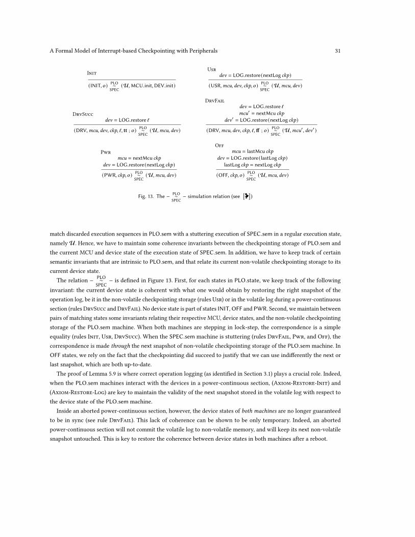
A Formal Model of Interrupt-based Checkpointing with Peripherals 31

Init

(INIT, 𝑜 ) PLO∼SPEC

(U,MCU.init,DEV.init)

Usr

dev = LOG.restore(nextLog ckp)

(USR,mcu, dev, ckp, 𝑜 ) PLO∼SPEC

(U,mcu, dev)

DrvSucc

dev = LOG.restore ℓ

(DRV,mcu, dev, ckp, ℓ, tt ; 𝑜 ) PLO∼SPEC

(U,mcu, dev)

DrvFail

dev = LOG.restore ℓmcu

′ = nextMcu ckpdev

′ = LOG.restore(nextLog ckp)

(DRV,mcu, dev, ckp, ℓ,ff ; 𝑜 ) PLO∼SPEC

(U,mcu′, dev′ )

Pwr

mcu = nextMcu ckpdev = LOG.restore(nextLog ckp)

(PWR, ckp, 𝑜 ) PLO∼SPEC

(U,mcu, dev)

Off

mcu = lastMcu ckpdev = LOG.restore(lastLog ckp)

lastLog ckp = nextLog ckp

(OFF, ckp, 𝑜 ) PLO∼SPEC

(U,mcu, dev)

Fig. 13. The − PLO∼SPEC

− simulation relation (see[ ]

)

match discarded execution sequences in PLO.sem with a stuttering execution of SPEC.sem in a regular execution state,

namely U. Hence, we have to maintain some coherence invariants between the checkpointing storage of PLO.sem and

the current MCU and device state of the execution state of SPEC.sem. In addition, we have to keep track of certain

semantic invariants that are intrinsic to PLO.sem, and that relate its current non-volatile checkpointing storage to its

current device state.

The relation − PLO∼SPEC

− is defined in Figure 13. First, for each states in PLO.state, we keep track of the following

invariant: the current device state is coherent with what one would obtain by restoring the right snapshot of the

operation log, be it in the non-volatile checkpointing storage (rules Usr) or in the volatile log during a power-continuous

section (rulesDrvSucc andDrvFail). No device state is part of states INIT,OFF and PWR. Second, we maintain between

pairs of matching states some invariants relating their respective MCU, device states, and the non-volatile checkpointing

storage of the PLO.sem machine. When both machines are stepping in lock-step, the correspondence is a simple

equality (rules Init, Usr, DrvSucc). When the SPEC.sem machine is stuttering (rules DrvFail, Pwr, and Off), the

correspondence is made through the next snapshot of non-volatile checkpointing storage of the PLO.sem machine. In

OFF states, we rely on the fact that the checkpointing did succeed to justify that we can use indifferently the next or

last snapshot, which are both up-to-date.

The proof of Lemma 5.9 is where correct operation logging (as identified in Section 3.1) plays a crucial role. Indeed,

when the PLO.sem machines interact with the devices in a power-continuous section, (Axiom-Restore-Init) and

(Axiom-Restore-Log) are key to maintain the validity of the next snapshot stored in the volatile log with respect to

the device state of the PLO.sem machine.

Inside an aborted power-continuous section, however, the device states of both machines are no longer guaranteed

to be in sync (see rule DrvFail). This lack of coherence can be shown to be only temporary. Indeed, an aborted

power-continuous section will not commit the volatile log to non-volatile memory, and will keep its next non-volatile

snapshot untouched. This is key to restore the coherence between device states in both machines after a reboot.

32 Gautier Berthou, Pierre-Évariste Dagand, Delphine Demange, Rémi Oudin, and Tanguy Risset

5.9 From PLF to SPEC

As illustrated in Figs. 7 and 9, our final Theorem 5.3 relates execution traces from PLF.sem down to SPEC.sem sub-traces,

through the relational composition of − ≽Log − and − ≽Ckp −. We prove Theorem 5.3 by simply chaining Lemmas 5.4,

5.5, 5.7 and 5.8 [ ].

5.10 Correctness with explicit trace filtering

We conclude this section by showing how Theorem 5.3 can be rephrased in a more operational way. Rather than proving

the existence of a SPEC trace related through − ≽ − to the initial PLF trace, we can show that the SPEC trace can be

explicitly extracted from the PLF trace, using a function filter, which (deterministically) filters out irrelevant portions

from the emitted trace.

Theorem 5.10 (Correctness with explicit trace filtering [ ]). For any trace t ∈ PLF.sem, we have filter(t) ∈SPEC.sem.

The definition of the filter function follows the intuition we give in Section 5, and is obtained by composing two

sub-filter functions, filterCkp and filterLog: the PLF trace is first cleared from the portions corresponding to failed

checkpoints (function filterCkp), and then cleared from the portions corresponding to aborted (and thus replayed)

power-continuous sections (function filterLog). Implementing those filter functions is straightforward. We refer to the

Coq development for further details. We prove that the filter function is correct with respect to the subtrace relation

− ≽ −:

Lemma 5.11 (The filter function is correct [ ]). For any trace t ∈ PLF.trace, t ≽ filter(t).

A significant advantage of this explicit, executable filter function is that it is more actionable than its relational

counterpart: it could e.g., be used by external users of a concrete implementation of a checkpointing scheme to test and

assess the functional correctness of their (checkpointed) application by analyzing filtered dumps of device operation

traces.

Interestingly, we derive the proof of Theorem 5.10 from Theorem 5.3 by simply proving that it is a complete

implementation of the subtrace relation − ≽ −:

Lemma 5.12 (The filter function is complete [ ]). For any traces t ∈ PLF.trace and t ∈ SPEC.trace, if t ≽ t, then

t = filter(t).

Lemma 5.12 is a direct consequence of Lemmas 5.11 and 5.2.

6 RELATEDWORK

Failure-atomicity run-times. In the general case, i.e., distributed systems with volatile and non-volatile RAM, ensuring

correctness and consistency of execution is a complex problem because volatile and non-volatile memories are out

of sync after a crash [42]. New programming models are proposed using locks [9, 12] or extended transactional

memory [15].

These legacy software systems provide minimally invasive change to programming models and environments, hence

they propose concurrency-like abstractions. These concepts have been used in the context of low-power transiently-

powered sensors [32, 39] that use NVM both for checkpointing and for regular program storage.

A Formal Model of Interrupt-based Checkpointing with Peripherals 33

Currently, our specification SPEC does not account for NVM state, hence we cannot model applications that assume

that part of the program memory, e.g., a stack, is in NVM.

Static and Interrupt-based checkpointing. Following the development of NVM and harvesting technologies [16, 18,

30, 40], numerous systems have been proposed to allow low-power sensors to be deployed in transiently-powered

environments. Among the most well-known are chronologically: Mementos [38], QuickRecall [26], Hibernus [3],

Dino [32], Ratchet [54], HarvOS [8], Clank [19], Alpaca [34] and Coati [39]. Most of these systems used checkpointing.

The insertion of checkpoints can be static [8, 32], dynamic [35, 54] or, when power failures can be detected by voltage

drop, interrupt-based [3, 7, 26]. The IBIS tool suite [45] is able to detect, statically or dynamically, memory inconsistencies

that may occur in these applications without relying on Assumption (A1) (i.e., the MCU may directly manipulate NVM).

Handling peripherals. Peripherals are not handled by classical checkpointing techniques. Peripherals are very

important in embedded computing and there is also, as for memory, a state consistency problem when power is

lost [32, 36]. Few systems have proposed a complete mechanism to ensure peripheral device restoration.

Sytare [6, 7] proposed a solution to recover the state of both the processor and the peripherals. Restop [2] solves a

similar problem with a middleware library for off-chip peripherals accessed by SPI or I2C. Karma [10] proposes another

implementation. These three approaches are captured by our checkpointing model and can benefit from the modeling

proposed here to verify their correctness.

Samoyed [36] proposes, under some restrictions (no interrupts allowed, stateless peripherals) to ensure peripheral

state consistency by introducing user-controlled atomicity. Being stateless, the peripherals considered by Samoyed do

not need a log to be restored. However, since Samoyed makes use of NVM in application code, it is not captured by our

current model.

Formal models, correctness proofs. Chen et al. [14] discuss some approaches for specifying and certifying crash-safety

for a persistent file system. The FSCQ system they later verified [13] uses a Hoare-logic style for specifying the system:

crash conditions specify the disk state right before a crash, and a recovery procedure ensures the absence of data loss.

A first difference between this line of work and ours is that we consider crash-safety in systems handling peripherals. A

second difference is in the general specification methodology. We adopt the so-called DSL approach [14]: we phrase the

specification and the model in terms of state machines and prove a refinement between the two. Chajed et al. [11] also

derive a refinement result from the Hoare-logic style specification. As they do not handle peripherals, their refinement

is a simple trace inclusion. In contrast, to derive a useful and precise correctness result, we must resort to a subtrace

relation.

Koskinen and Yang [28] also employ a DSL approach. Interestingly, their notion of recoverability is expressed in

terms of an un-crashed program: after a crash, the program will eventually reach a state that simulates another state

that an un-crashed program already reached (i.e., in the trace prefix). In our model, instrumented traces and the subtrace

relation help us state simply to which prefix it corresponds.

Another line of work focuses on proving the linearizability of fine-grained concurrent data-structures subject to

whole-system crash [17, 25].Durable linearizability requires that upon a crash, only completed operations are guaranteed

to remain visible. Buffered durable linearizability expresses that the state after the crash must be consistent, but not

necessarily up-to-date. Our subtrace refinement result is similar in spirit to a buffered durable linearization property.

Independently to our own effort, Surbatovich et al. [46] has proposed a formal model of intermittent computing

that accounts for peripherals. The model aims at reasoning about the error-prone interaction between persistent

34 Gautier Berthou, Pierre-Évariste Dagand, Delphine Demange, Rémi Oudin, and Tanguy Risset

application variables (which we side-stepped through our Assumption (A1)) and performing repeated device or sensor

inputs (dubbed “RIO” in the paper). The resulting model is orthogonal to ours as it explicitly does not try to take into

account timeliness nor interrupts [46, §2.1]. It would be quite appealing to integrate both results in a single, conceptual

framework.

7 CONCLUSION

We proposed a specification of intermittent computing with peripherals, together with a model of interrupt-based

checkpointing that ensures the consistency of the whole system, i.e., including peripherals, after reboot. Our model

contains the minimal conditions that an implementation of checkpointing should satisfy to handle peripherals cor-

rectly. We formally proved the correctness of our model: behaviors of intermittent executions are as prescribed by a

continuously-powered specification, modulo the necessary replays of certain peripheral operations, due to reboots.

Finally, we showed that our model captures three proposals satisfying our working assumptions (A1-4): Restop [2],

Sytare [7] and Karma [10].

Throughout this work, we have assumed that the application code does not interact with non-volatile memory (A1).

We are currently working on extending our specification and our checkpointing model to account for NVM application

state. This would allow us to model more systems from the literature [19, 32, 34, 36, 54].

ACKNOWLEDGMENTS

We would like to thank the anonymous reviewers for their thoughtful comments. This work was supported by Inria

(IPL ZEP) and the Émergence(s) program of the City of Paris.

REFERENCES[1] Saad Ahmed, Naveed Anwar Bhatti, Muhammad Hamad Alizai, Junaid Haroon Siddiqui, and Luca Mottola. 2019. Efficient Intermittent Computing

with Differential Checkpointing. In Proceedings of the 20th ACM SIGPLAN/SIGBED International Conference on Languages, Compilers, and Tools for

Embedded Systems (Phoenix, AZ, USA) (LCTES 2019). Association for Computing Machinery, New York, NY, USA, 70–81. https://doi.org/10.1145/

3316482.3326357

[2] Alberto Rodriguez Arreola, Domenico Balsamo, Geoff V. Merrett, and Alex S. Weddell. 2018. RESTOP: Retaining External Peripheral State in

Intermittently-Powered Sensor Systems. Sensors 18, 1 (2018), 172. https://doi.org/10.3390/s18010172

[3] Domenico Balsamo, Alex S. Weddell, Geoff V. Merrett, Bashir M. Al-Hashimi, Davide Brunelli, and Luca Benini. 2015. Hibernus: Sustaining

Computation During Intermittent Supply for Energy-Harvesting Systems. Embedded Systems Letters 7, 1 (2015), 15–18. https://doi.org/10.1109/LES.

2014.2371494

[4] Gautier Berthou, Pierre-Évariste Dagand, Delphine Demange, Rémi Oudin, and Tanguy Risset. 2020. Intermittent Computing with Peripherals,

Formally Verified. In Proceedings of the 21st ACM SIGPLAN/SIGBED International Conference on Languages, Compilers, and Tools for Embedded

Systems, LCTES 2020, London, UK, June 16, 2020. 85–96. https://doi.org/10.1145/3372799.3394365

[5] Gautier Berthou, Pierre-Evariste Dagand, Delphine Demange, Rémi Oudin, and Tanguy Risset. 2020. Intermittent Computing with Peripherals,

Formally Verified – Companion Coq Development. https://gabertho.gitlabpages.inria.fr/icp-model/

[6] Gautier Berthou, Tristan Delizy, Kevin Marquet, Tanguy Risset, and Guillaume Salagnac. 2017. Peripheral state persistence for transiently-powered

systems. In Global Internet of Things Summit (GIoTS). IEEE, New York, NY, USA, 1–6. https://doi.org/10.1109/GIOTS.2017.8016243

[7] Gautier Berthou, Tristan Delizy, Kevin Marquet, Tanguy Risset, and Guillaume Salagnac. 2019. Sytare: A Lightweight Kernel for NVRAM-Based

Transiently-Powered Systems. IEEE Trans. Comput. 68, 9 (Sep. 2019), 1390–1403.

[8] Naveed Anwar Bhatti and Luca Mottola. 2017. HarvOS: Efficient Code Instrumentation for Transiently-Powered Embedded Sensing. In Proceedings

of the 16th ACM/IEEE International Conference on Information Processing in Sensor Networks (Pittsburgh, Pennsylvania) (IPSN ’17). Association for

Computing Machinery, New York, NY, USA, 209–219.

[9] Hans-J. Boehm and Dhruva R. Chakrabarti. 2016. Persistence Programming Models for Non-Volatile Memory. SIGPLAN Not. 51, 11 (June 2016),

55–67. https://doi.org/10.1145/3241624.2926704

[10] Adriano Branco, Luca Mottola, Muhammad Hamad Alizai, and Junaid Haroon Siddiqui. 2019. Intermittent Asynchronous Peripheral Operations. In

Proceedings of the 17th Conference on Embedded Networked Sensor Systems (New York, New York) (SenSys ’19). Association for Computing Machinery,

New York, NY, USA, 55–67.

A Formal Model of Interrupt-based Checkpointing with Peripherals 35

[11] Tej Chajed, Joseph Tassarotti, M. Frans Kaashoek, and Nickolai Zeldovich. 2019. Verifying Concurrent, Crash-Safe Systems with Perennial. In

Proceedings of the 27th ACM Symposium on Operating Systems Principles (Huntsville, Ontario, Canada) (SOSP ’19). Association for Computing

Machinery, New York, NY, USA, 243–258. https://doi.org/10.1145/3341301.3359632

[12] Dhruva R. Chakrabarti, Hans-J. Boehm, and Kumud Bhandari. 2014. Atlas: Leveraging Locks for Non-Volatile Memory Consistency. SIGPLAN Not.

49, 10 (Oct. 2014), 433–452.

[13] Haogang Chen, Daniel Ziegler, Tej Chajed, Adam Chlipala, M. Frans Kaashoek, and Nickolai Zeldovich. 2015. Using Crash Hoare Logic for Certifying

the FSCQ File System. In Proceedings of the 25th Symposium on Operating Systems Principles (Monterey, California) (SOSP ’15). Association for

Computing Machinery, New York, NY, USA, 18–37. https://doi.org/10.1145/2815400.2815402

[14] Haogang Chen, Daniel Ziegler, Adam Chlipala, M. Frans Kaashoek, Eddie Kohler, and Nickolai Zeldovich. 2015. Specifying Crash Safety for Storage

Systems. In Proceedings of the 15th USENIX Conference on Hot Topics in Operating Systems (Switzerland) (HOTOS’15). USENIX Association, USA, 21.

[15] Joel Coburn, Adrian M. Caulfield, Ameen Akel, Laura M. Grupp, Rajesh K. Gupta, Ranjit Jhala, and Steven Swanson. 2011. NV-Heaps: Making

Persistent Objects Fast and Safe with next-Generation, Non-Volatile Memories. SIGARCH Comput. Archit. News 39, 1 (March 2011), 105–118.

[16] Alexei Colin, Emily Ruppel, and Brandon Lucia. 2018. A Reconfigurable Energy Storage Architecture for Energy-harvesting Devices. In Proceedings

of the Twenty-Third International Conference on Architectural Support for Programming Languages and Operating Systems (ASPLOS ’18). ACM, New

York, NY, USA, 767–781.

[17] John Derrick, Simon Doherty, Brijesh Dongol, Gerhard Schellhorn, and Heike Wehrheim. 2019. Verifying Correctness of Persistent Concurrent

Data Structures. In Formal Methods – The Next 30 Years, Maurice H. ter Beek, Annabelle McIver, and José N. Oliveira (Eds.). Springer International

Publishing, Cham, Switzerland, 179–195.

[18] Josiah Hester, Kevin Storer, and Jacob Sorber. 2017. Timely Execution on Intermittently Powered Batteryless Sensors. In Proceedings of the 15th

ACM Conference on Embedded Network Sensor Systems (Delft, Netherlands) (SenSys ’17). ACM, New York, NY, USA, Article 17, 13 pages.

[19] Matthew Hicks. 2017. Clank: Architectural Support for Intermittent Computation. SIGARCH Comput. Archit. News 45, 2 (June 2017), 228–240.

[20] Texas Instruments. 2019. MSP430FR2433 Mixed-Signal Microcontroller. https://www.ti.com/lit/ds/slase59f/slase59f.pdf

[21] Texas Instruments. 2019. MSP430FR4xx and MSP430FR2xx family User’s Guide. http://ti.com/lit/ug/slau445i/slau445i.pdf

[22] Texas Instruments. 2020. CC1101: low-Power sub-1 GHz RF transceiver. https://www.ti.com/lit/ds/symlink/cc1101.pdf

[23] Texas Instruments. 2020. CC2500 Low-Cost Low-Power 2.4 GHz RF Transceiver. https://www.ti.com/lit/ds/swrs040c/swrs040c.pdf

[24] Intersil. 2011. ISL29004: Light-to-Digital Output Sensor. https://datasheetspdf.com/pdf-file/584086/IntersilCorporation/ISL29004/1

[25] Joseph Izraelevitz, Hammurabi Mendes, and Michael L. Scott. 2016. Linearizability of Persistent Memory Objects Under a Full-System-Crash Failure

Model. In Distributed Computing, Cyril Gavoille and David Ilcinkas (Eds.). Springer Berlin Heidelberg, Berlin, Heidelberg, 313–327.

[26] Hrishikesh Jayakumar, Arnab Raha, Woo Suk Lee, and Vijay Raghunathan. 2015. QuickRecall: A HW/SW Approach for Computing across Power

Cycles in Transiently Powered Computers. JETC 12, 1 (2015), 8:1–8:19. https://doi.org/10.1145/2700249

[27] Knowles. 2014. SPW2430HR5H-B: Top Port SiSonic Microphone. https://www.knowles.com/docs/default-source/model-downloads/spw2430hr5h-

b.pdf

[28] Eric Koskinen and Junfeng Yang. 2016. Reducing Crash Recoverability to Reachability. In Proceedings of the 43rd Annual ACM SIGPLAN-SIGACT

Symposium on Principles of Programming Languages (St. Petersburg, FL, USA) (POPL ’16). Association for Computing Machinery, New York, NY,

USA, 97–108. https://doi.org/10.1145/2837614.2837648

[29] Leslie Lamport. 2008. Computation and state machines.

[30] Yoonmyung Lee, Suyoung Bang, Inhee Lee, Yejoong Kim, Gyouho Kim, Mohammad Hassan Ghaed, Pat Pannuto, Prabal Dutta, Dennis Sylvester,

and David Blaauw. 2013. A Modular 1 mm3Die-Stacked Sensing Platform With Low Power I

2C Inter-Die Communication and Multi-Modal Energy

Harvesting. IEEE Journal of Solid-State Circuits 48 (2013), 229–243.

[31] Xavier Leroy. 2009. A Formally Verified Compiler Back-End. J. Autom. Reason. 43, 4 (Dec. 2009), 363–446. https://doi.org/10.1007/s10817-009-9155-4

[32] Brandon Lucia and Benjamin Ransford. 2015. A simpler, safer programming and execution model for intermittent systems. In Proceedings of the 36th

ACM SIGPLAN Conference on Programming Language Design and Implementation, Portland, OR, USA, June 15-17, 2015. ACM, Portland, OR, USA,

575–585.

[33] Nancy Lynch and Frits Vaandrager. 1996. Forward and Backward Simulations. Inf. Comput. 128, 1 (July 1996), 1–25. https://doi.org/10.1006/inco.

1996.0060

[34] Kiwan Maeng, Alexei Colin, and Brandon Lucia. 2017. Alpaca: intermittent execution without checkpoints. PACMPL 1, OOPSLA (2017), 96:1–96:30.

https://doi.org/10.1145/3133920

[35] Kiwan Maeng and Brandon Lucia. 2018. Adaptive Dynamic Checkpointing for Safe Efficient Intermittent Computing. In 13th USENIX Symposium on

Operating Systems Design and Implementation, OSDI 2018, Carlsbad, CA, USA, October 8-10, 2018. USENIX Association, Carlsbad, CA, 129–144.

[36] Kiwan Maeng and Brandon Lucia. 2019. Supporting peripherals in intermittent systems with just-in-time checkpoints. In Proceedings of the 40th

ACM SIGPLAN Conference on Programming Language Design and Implementation, PLDI 2019, Phoenix, AZ, USA, June 22-26, 2019. ACM, New York,

NY, USA, 1101–1116.

[37] Benjamin Ransford and Brandon Lucia. 2014. Nonvolatile Memory is a Broken Time Machine. In Proceedings of the Workshop on Memory Systems

Performance and Correctness (Edinburgh, United Kingdom) (MSPC ’14). Association for Computing Machinery, New York, NY, USA, Article 5, 3 pages.

https://doi.org/10.1145/2618128.2618136

36 Gautier Berthou, Pierre-Évariste Dagand, Delphine Demange, Rémi Oudin, and Tanguy Risset

[38] Benjamin Ransford, Jacob Sorber, and Kevin Fu. 2011. Mementos: system support for long-running computation on RFID-scale devices. In

International Conference on Architectural Support for Programming Languages and Operating Systems (ASPLOS) (Newport Beach, California, USA).

ACM, New York, NY, USA, 159–170.

[39] Emily Ruppel and Brandon Lucia. 2019. Transactional concurrency control for intermittent, energy-harvesting computing systems. In Proceedings of

the 40th ACM SIGPLAN Conference on Programming Language Design and Implementation, PLDI 2019, Phoenix, AZ, USA, June 22-26, 2019, Kathryn S.

McKinley and Kathleen Fisher (Eds.). ACM, New York, NY, USA, 1085–1100. https://doi.org/10.1145/3314221.3314583

[40] Alanson P. Sample, Daniel J. Yeager, Pauline S. Powledge, Alexander V. Mamishev, and Joshua R. Smith. 2008. Design of an RFID-Based Battery-Free

Programmable Sensing Platform. IEEE Transactions on Instrumentation and Measurement 57, 11 (2008), 2608–2615.

[41] Sensirion. 2011. SHT1x: Humidity and Temperature Sensor IC. https://www.sensirion.com/fileadmin/user_upload/customers/sensirion/Dokumente/

2_Humidity_Sensors/Datasheets/Sensirion_Humidity_Sensors_SHT1x_Datasheet.pdf

[42] Thomas Shull, Jian Huang, and Josep Torrellas. 2018. Defining a high-level programming model for emerging NVRAM technologies. In Proceedings of

the 15th International Conference on Managed Languages & Runtimes, ManLang 2018, Linz, Austria, September 12-14, 2018, Eli Tilevich and Hanspeter

Mössenböck (Eds.). ACM, New York, NY, USA, 11:1–11:7. https://doi.org/10.1145/3237009.3237027

[43] ST. 2017. LIS3MDL: digital output magnetic sensor. https://www.st.com/resource/en/datasheet/lis3mdl.pdf

[44] ST. 2017. LSM6DSL: iNEMO inertial module. https://www.st.com/resource/en/datasheet/lsm6dsl.pdf

[45] Milijana Surbatovich, Limin Jia, and Brandon Lucia. 2019. I/O dependent idempotence bugs in intermittent systems. PACMPL 3, OOPSLA (2019),

183:1–183:31. https://doi.org/10.1145/3360609

[46] Milijana Surbatovich, Limin Jia, and Brandon Lucia. 2020. Towards a Formal Foundation of Intermittent Computing. PACMPL OOPSLA (2020).

[47] Sytare. 2020. CC2500 driver. https://gitlab.inria.fr/citi-lab/sytare-public/-/blob/isr/src/drivers/cc2500.c

[48] Sytare. 2020. Clock driver. https://gitlab.inria.fr/citi-lab/sytare-public/-/blob/isr/src/drivers/clock.c

[49] Sytare. 2020. GPIO driver. https://gitlab.inria.fr/citi-lab/sytare-public/-/blob/isr/src/drivers/port.c

[50] Sytare. 2020. SPI driver. https://gitlab.inria.fr/citi-lab/sytare-public/-/blob/isr/src/drivers/spi.c

[51] Sytare. 2020. Temperature sensor driver. https://gitlab.inria.fr/citi-lab/sytare-public/-/blob/isr/src/drivers/temperature.c

[52] Sytare. 2020. Timer driver. https://gitlab.inria.fr/citi-lab/sytare-public/-/blob/isr/src/drivers/timer.c

[53] The Coq Development Team. 2018. The Coq Proof Assistant, version 8.8.0. https://doi.org/10.5281/zenodo.1219885

[54] Joel van der Woude and Matthew Hicks. 2016. Intermittent Computation without Hardware Support or Programmer Intervention. In 12th USENIX

Symposium on Operating Systems Design and Implementation, OSDI 2016, Savannah, GA, USA, November 2-4, 2016. USENIX Association, Savannah,

GA, 17–32.