September 8, 2009 15:42 WSPC/214-IJSC - SPI-J091 00071

International Journal of Semantic ComputingVol. 3, No. 2 (2009) 183–208c© World Scientific Publishing Company

A FEATURE SELECTION APPROACH FOR AUTOMATICMUSIC GENRE CLASSIFICATION

CARLOS N. SILLA JR.

Computing Laboratory, University of KentCanterbury, CT2 7NF, Kent, UK

cns2@kent.ac.uk

ALESSANDRO L. KOERICH

Pontifical Catholic University of ParanaR. Imaculada Conceicao 1155, 80215-901, Curitiba, PR, Brazil

alekoe@ppgia.pucpr.br

CELSO A. A. KAESTNER

Federal University of Technology of ParanaAv. Sete de Setembro 3165, 80230-901, Curitiba, PR, Brazil

kaestner@dainf.ct.utfpr.edu.br

In this paper we present an analysis of the suitability of four different feature sets whichare currently employed to represent music signals in the context of the automatic musicgenre classification. To such an aim, feature selection is carried out through genetic algo-rithms, and it is applied to multiple feature vectors generated from different segments ofthe music signal. The feature sets used in this paper, which encompass time-domain andfrequency-domain characteristics of the music signal, comprise: short-time Fourier trans-form, Mel frequency cepstral coefficient, beat-related features, pitch-related features,inter-onset interval histogram coefficients, rhythm histograms and statistical spectrumdescriptors. The classification is based on the use of multiple feature vectors and anensemble approach, according to time and space decomposition strategies. Feature vec-tors are extracted from music segments from the beginning, middle and end parts of themusic signal (time-decomposition). Despite music genre classification being a multi-classproblem, we accomplish the task using a combination of binary classifiers, whose resultsare merged to produce the final music genre label (space decomposition). Experimentswere carried out on two databases: the Latin Music Database, which contains 3,227music pieces categorized into ten musical genres; the ISMIR’2004 genre contest databasewhich contains 1,458 music pieces categorized into six popular western musical genres.The experimental results have shown that the feature sets have different importanceaccording to the part of the music signal from where the feature vectors are extracted.

Furthermore, the ensemble approach provides better results than the individual seg-ments in most cases. For high-dimensional feature sets, the feature selection providesa compact but discriminative feature subset which has an interesting trade-off betweenclassification accuracy and computational effort.

Keywords: Music classification; feature selection; audio processing.

183

September 8, 2009 15:42 WSPC/214-IJSC - SPI-J091 00071

184 C. N. Silla Jr., A. L. Koerich & C. A. A. Kaestner

1. Introduction

Music genres can be defined as categorical labels created by humans to identify orcharacterize the style of music. In spite of the lack of standards, assigning a genre toa music piece is difficult, due to human perception subjectiveness. However musicgenre is an important descriptor which is widely used to organize and managelarge digital music databases and electronic music distribution (EMD) [1, 30, 42].Furthermore, on the Internet which contains large amounts of multimedia content,musical genres are frequently used in search queries [8, 18].

Nowadays the standard procedure for sorting and organizing music content isbased on meta information tags such as the ID3 tags, which are usually associatedwith music coded in the MPEG-1 Audio Layer 3 (MP3) audio-specific compressionformat [14]. The ID3 tags are a section of the compressed MP3 audio file that con-tains meta information about the music. This metadata includes song title, artist,album, year, track number and music genre, besides other information about thefile contents. As of 2009, the most widespread standard tag formats are ID3v1 andID3v2. Although the ID3 tags contain relevant information for indexing, searchingand retrieving digital music, they are often incomplete or inaccurate. For this rea-son, a tool that is able to classify musical genres in an automatic fashion relying onlyon the music contents will play an important role in any music information retrievalsystem. The scientific aspect of the problem is also an issue, since automatic musicgenre classification (AMGC) can be posed, from a pattern recognition perspective,as an interesting research problem: the music signal is a highly dimensional complextime-variant signal and the music databases can be very large [2].

Any approach that deals with automatic music genre classification has to findan adequate representation of the music signal to allow further processing throughdigital machines. For such an aim, a feature extraction procedure is applied tothe music signal to obtain a compact and discriminant representation in termsof a feature vector. Then, it becomes straightforward to tackle this problem asa classical classification task in a pattern recognition framework [28]. Typically amusic database contains thousands of pieces from dozens of manually-defined musicgenres [1, 23, 35], characterizing a complex multi-class classification problem.

Results on classification, however, depend strongly on the extracted featuresand their ability to discriminate the classes. It has been observed that beyonda certain point, the inclusion of additional features leads to a worse rather thanbetter performance. Moreover, the choice of features to represent the patterns affectsimportant aspects of the classification such as accuracy, required learning time, andthe necessary number of samples. Such a problem refers to the task of identifying andselecting a proper subset of original feature set, in order to simplify and reduce theeffort in preprocessing and classifying, while assuring similar or higher classificationaccuracy than the complete feature set [3, 6].

In this paper we present an analysis of the suitability of four feature sets whichare currently employed to represent music signals in the context of AMGC. To such

September 8, 2009 15:42 WSPC/214-IJSC - SPI-J091 00071

A Feature Selection Approach for Automatic Music Genre Classification 185

an aim, feature selection is carried out through genetic algorithms (GA). The fea-tures employed in this paper comprise short-time Fourier transform, Mel frequencycepstral coefficients (MFCC), beat and pitch related features [42], inter-onset inter-val histogram coefficients (IOIHC) [13], rhythm histograms (RH) and statisticalspectrum descriptors (SSD) [24, 31, 32]. We also use a non-conventional classifica-tion approach that employs ensemble of classifiers [7,16], and which is based on timeand space decomposition schemes that produce multiple feature vectors from a sin-gle music signal. The feature selection algorithm is applied to the multiple featuresvectors allowing a comparison of the relative importance of the features accordingto the segment of the music signal from where it was extracted, the feature setitself, as well as an analysis of the impact of the feature selection on the musicgenre classification. Principal Component Analysis (PCA) procedure is also consid-ered for comparison purposes. The experiments were carried out on two databases:ISMIR’2004 database [4, 15], and Latin Music Database (LMD) [38].

This paper is organized as follows. Section 2 presents the AMGC problem for-malization and summarizes related works in feature selection. Section 3 presents thetime/space decomposition strategies used in our AMGC system. Section 4 describesthe different feature sets used in this work as well as the feature selection procedurebased on GA. Section 5 describes the databases used in the experiments as well asthe results achieved while using feature selection over multiple feature vectors fromdifferent feature sets. Finally, the conclusions are stated in the last section.

2. Problem Definition and Related Work

Sound is usually considered as a mono-dimensional signal representing the air pres-sure in the ear canal [33]. In digital audio, the representation of the sound is nolonger directly analogous to the sound wave. The signal must be reduced to discretesamples of a discrete-time domain. Therefore, the continuous-time signal, denotedas y(t), is sampled at time instants that are multiple of a quantity T , called thesampling interval. Sampling a continuous-time signal y(t) with sampling intervalT produces a function s(n) = y(nT ) of the discrete variable n, which represents adigital audio signal [33].

A significant amount of acoustic information is embedded in such a digital musicsignal. This spectral information can be represented in terms of features. From thepattern recognition point of view we assume that a digital music signal, denotedas s(n), is represented by a set of features. If we consider d features, s(n) can berepresented by a d-dimensional feature vector denoted as x and represented as

x = [x1, . . . , xd]T ∈ d (1)

where each component xi ∈ d represents a vector component extracted from s(n).We shall assume that there are c possible labeled classes organized as a set of

labels Ω = [ω1, . . . , ωc] and that each digital music signal belongs to one and onlyone class. Considering that our aim is to classify music according to its genre, then

September 8, 2009 15:42 WSPC/214-IJSC - SPI-J091 00071

186 C. N. Silla Jr., A. L. Koerich & C. A. A. Kaestner

the classification problem consists in assigning a musical genre ωj ∈ Ω which betterrepresents s(n). This problem can be framed from a statistical perspective wherethe goal is to find the musical genre ωj that is most likely, given a feature vector x

extracted from s(n); that is, the musical genre with the largest posterior probability,denoted as ω

ω = argmaxωj∈Ω

P (ωj |x) (2)

where P (ωj|x) is the a posteriori probability of a music genre ωj given a featurevector x. This probability can be rewritten using Bayes’ rule

P (ωj|x) =P (x|ωj)P (ωj)

P (x)(3)

where P (ωj) is the a priori probability of the musical genre, which is estimatedfrom frequency counts in a data set. The probability of data occurring P (x) isunknown, but assuming that the genre ωj ∈ Ω and that the classifier computes thelikelihoods of the entire set of possible hypotheses (all musical genres in Ω), thenthe probabilities must sum to one∑

ωj∈Ω

P (ωj |x) = 1. (4)

In such a way, estimated a posteriori probabilities can be used as confidenceestimates [41]. Then, we obtain the posterior P (ωj |x) for the music genre hypotheses

P (ωj|x) =P (x|ωj)P (ωj)∑

ωj∈ΩP (x|ωj)P (ωj). (5)

Feature selection can be easily incorporated in this description. Assuming asubset of d′ features, where d′ < d, then d′

is a projection of d. Let us denote x′

as a projection of the feature vector x, then we want to select an adequate x′ suchthat it simplifies the decision

ω = argmaxωj∈Ω

P (x′|ωj)P (ωj)∑ωj∈ΩP (x′|ωj)P (ωj)

. (6)

Also, since x′ has a lower dimension than x, it can be computed faster than x.The issue of automatic music genre classification as a pattern recognition prob-

lem has been brought up in the work of Tzanetakis and Cook [42]. In this work theyuse a comprehensive set of features to represent a music piece, including timbraltexture features, beat-related features and pitch-related features. These featureshave become of public use, as part of the MARSYAS framework,a an open soft-ware platform for digital audio applications. Tzanetakis and Cook have used Gaus-sian classifiers, Gaussian mixture models and k Nearest-Neighbors (k-NN) classifierstogether with feature vectors extracted from the first 30 seconds of the music pieces.They have developed a database named GTZAN which comprises 1,000 samples of

aMusic Analysis, Retrieval and SYnthesis for Audio Signals, available at http://marsyas.sourge-forge.net/

September 8, 2009 15:42 WSPC/214-IJSC - SPI-J091 00071

A Feature Selection Approach for Automatic Music Genre Classification 187

music pieces from ten music genres (classical, country, disco, hiphop, jazz, rock,blues, reggae, pop, metal). Using the full feature set (timbral + rhythm + pitch)and a ten-fold cross validation procedure, they have achieved correct music genreclassification with 60% accuracy.

Most of the current research on music genre classification focuses on the develop-ment of new feature sets and classification methods [17,21–23,27]. A more detaileddescription and comparison of these works can be found in [39]. On the other hand,few works have dealt with feature selection. One of the few exceptions is the workof Grimaldi et al. [10, 11]. The authors decompose the original problem accordingto an ensemble approach, employing different feature selection procedures, suchas ranking according to the information gain (IG), ranking according to the gainratio (GR), and principal component analysis (PCA). In the experiments they haveused two hundred music pieces from five music genres, together with a k-NN clas-sifier and a five-fold cross validation procedure. The feature vector was generatedfrom the entire music piece using discrete periodic wavelet transform (DPWT). ThePCA approach proves to be the most effective feature selection technique, achiev-ing an accuracy of 79% with the k-NN classifier. The space decomposition approachachieved 81% for both the IG and the GR feature selection procedures, showing itto be an effective ensemble technique. When applying a forward sequential fea-ture selection based on the GR ranking, the ensemble achieved is 84%. However,no experiments have been carried out using a standard feature set, like the oneproposed by Tzanetakis and Cook [42].

Fiebrink & Fujinaga [9] discuss the use of complex feature representation andthe necessary computational resources to compute them. They have employed 74low-level features available at the jAudio [20]. jAudio is a software package forextracting features from audio files as well as for iteratively developing and sharingnew features. Then, these features can be used in many areas of music informationretrieval (MIR) research. To evaluate feature selection in the AMGC problem theyhave employed a forward feature selection (FFS) procedure and also a principalcomponent analysis (PCA) procedure. The experiments were carried out using theMagnatune database (4,476 music pieces from 24 genres) [19] and the results overa testing set indicate that accuracy rises from 61.2% without feature selection to69.8% with FFS and 71% with PCA.

Yaslan and Cataltepe [44] have also employed a feature selection approach formusic genre classification using search methods, such as forward feature selection(FFS) and backward feature selection (BFS). FFS and BFS methods are basedon a guided search in the feature space, starting from an empty set and from theentire set of features, respectively. Several classifiers were used in the experimentssuch as linear and quadratic discriminant classifiers, Naıve-Bayes, and variations ofthe k-NN classifier. They have employed the GTZAN database and the MARSYASframework for feature extraction [42]. The experimental results have shown thatfeature selection, the use of different classifiers, and a subsequent combination ofresults can improve the music genre classification accuracy.

September 8, 2009 15:42 WSPC/214-IJSC - SPI-J091 00071

188 C. N. Silla Jr., A. L. Koerich & C. A. A. Kaestner

Bergstra et al. [2] use AdaBoost which performs the classification iteratively bycombining the weighted votes of several weak learners. The feature vectors werebuilt from several features like fast Fourier transform coefficients, real cepstralcoefficients, MFCCs, zero-crossing rate, spectral spread, centroid, rolloff and auto-regression coefficients. Experiments were conducted considering the music genreidentification task and the artist identification task of the 2005 Music InformationRetrieval EXchange competition (MIREX’05). The proposed ensemble approachhave shown to be effective in three music genre databases. The best accuracies inthe case of the music genre identification problem vary from 75.10% to 86.92%.This result allowed the authors to win the task of music genre identification in theMIREX’05 competition.

In this paper we present a different approach to analyze the suitability of dif-ferent feature sets which are currently employed to represent music signals. Theproposed approach for feature selection is based on genetic algorithms. The mainreason for the use of genetic algorithm in feature selection instead of other tech-niques such as PCA, is that the use of feature selection mechanisms based on fea-ture transformation might improve the predictive accuracy, but limits the quality ofresults from a musicological perspective, as it loses potentially meaningful informa-tion about which musical qualities are most useful in different contexts, as pointedout by McKay and Fujinaga [26].

3. Music Classification: The Time/Space Decomposition Approach

The assignment of a genre to a given music piece can be considered as a threestep process [2]: (a) the extraction of acoustic features from short frames of theaudio signal; (b) the aggregation of the features into more abstract segment-levelfeatures; and (c) the prediction of the music genre using a class decision procedurethat uses the segment-level features as input. We emphasize that if we follow theclassical machine learning approach, the decision procedure is obtained from thetraining/validation/test cycle over a labeled database [28].

The AMGC system is based on standard supervised machine learning algo-rithms. However, we employ multiple feature vectors obtained from the originalmusic signal according to time and space decompositions [5, 34, 36]. We follow anensemble approach in which the final class label for the AMGC problem is producedas follows [25]: (a) feature vectors are obtained from several segments extracted fromthe music signal; (b) component classifiers are applied to each one of these featurevectors, providing a set of partial classification results; (c) a combination procedureis employed to produce the final class label from these partial classifications.

3.1. Time decomposition

Since music is a time-varying signal, time decomposition is obtained by consideringfeature vectors extracted from different temporal parts of the music signal. In thiswork we employ three segments, one from the beginning, one from the middle and

September 8, 2009 15:42 WSPC/214-IJSC - SPI-J091 00071

A Feature Selection Approach for Automatic Music Genre Classification 189

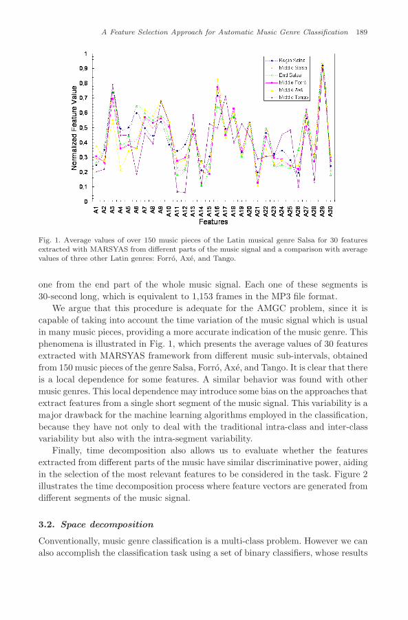
Fig. 1. Average values of over 150 music pieces of the Latin musical genre Salsa for 30 featuresextracted with MARSYAS from different parts of the music signal and a comparison with averagevalues of three other Latin genres: Forro, Axe, and Tango.

one from the end part of the whole music signal. Each one of these segments is30-second long, which is equivalent to 1,153 frames in the MP3 file format.

We argue that this procedure is adequate for the AMGC problem, since it iscapable of taking into account the time variation of the music signal which is usualin many music pieces, providing a more accurate indication of the music genre. Thisphenomena is illustrated in Fig. 1, which presents the average values of 30 featuresextracted with MARSYAS framework from different music sub-intervals, obtainedfrom 150 music pieces of the genre Salsa, Forro, Axe, and Tango. It is clear that thereis a local dependence for some features. A similar behavior was found with othermusic genres. This local dependence may introduce some bias on the approaches thatextract features from a single short segment of the music signal. This variability is amajor drawback for the machine learning algorithms employed in the classification,because they have not only to deal with the traditional intra-class and inter-classvariability but also with the intra-segment variability.

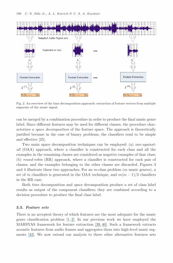
Finally, time decomposition also allows us to evaluate whether the featuresextracted from different parts of the music have similar discriminative power, aidingin the selection of the most relevant features to be considered in the task. Figure 2illustrates the time decomposition process where feature vectors are generated fromdifferent segments of the music signal.

3.2. Space decomposition

Conventionally, music genre classification is a multi-class problem. However we canalso accomplish the classification task using a set of binary classifiers, whose results

September 8, 2009 15:42 WSPC/214-IJSC - SPI-J091 00071

190 C. N. Silla Jr., A. L. Koerich & C. A. A. Kaestner

Fig. 2. An overview of the time decomposition approach: extraction of feature vectors from multiplesegments of the music signal.

can be merged by a combination procedure in order to produce the final music genrelabel. Since different features may be used for different classes, the procedure char-acterizes a space decomposition of the feature space. The approach is theoreticallyjustified because in the case of binary problems, the classifiers tend to be simpleand effective [25].

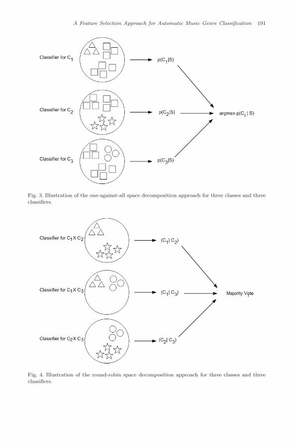
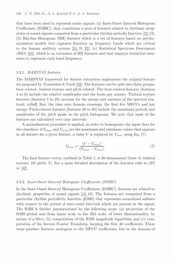
Two main space decomposition techniques can be employed: (a) one-against-all (OAA) approach, where a classifier is constructed for each class and all theexamples in the remaining classes are considered as negative examples of that class;(b) round-robin (RR) approach, where a classifier is constructed for each pair ofclasses, and the examples belonging to the other classes are discarded. Figures 3and 4 illustrate these two approaches. For an m-class problem (m music genres), aset of m classifiers is generated in the OAA technique, and m(m − 1)/2 classifiersin the RR case.

Both time decomposition and space decomposition produce a set of class labelresults as output of the component classifiers; they are combined according to adecision procedure to produce the final class label.

3.3. Feature sets

There is no accepted theory of which features are the most adequate for the musicgenre classification problem [1, 2]. In our previous work we have employed theMARSYAS framework for feature extraction [39, 40]. Such a framework extractsacoustic features from audio frames and aggregates them into high-level music seg-ments [42]. We now extend our analysis to three other alternative features sets

September 8, 2009 15:42 WSPC/214-IJSC - SPI-J091 00071

A Feature Selection Approach for Automatic Music Genre Classification 191

Fig. 3. Illustration of the one-against-all space decomposition approach for three classes and threeclassifiers.

Fig. 4. Illustration of the round-robin space decomposition approach for three classes and threeclassifiers.

September 8, 2009 15:42 WSPC/214-IJSC - SPI-J091 00071

192 C. N. Silla Jr., A. L. Koerich & C. A. A. Kaestner

that have been used to represent music signals: (a) Inset-Onset Interval HistogramCoefficients (IOIHC), that constitutes a pool of features related to rhythmic prop-erties of sound signals computed from a particular rhythm periodic function [12,13];(b) Rhythm Histogram (RH) features which is a set of features based on psycho-acoustical models that captures flotation on frequency bands which are criticalto the human auditory system [24, 31, 32]; (c) Statistical Spectrum Descriptors(SSD) [24], which is an extension of RH features and that employs statistical mea-sures to represent each band frequency.

3.3.1. MARSYAS features

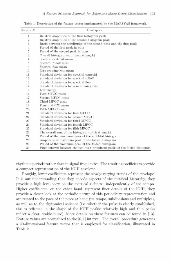
The MARSYAS framework for feature extraction implements the original featureset proposed by Tzanetakis & Cook [42]. The features can be split into three groups:beat related, timbral texture and pitch related. The beat-related features (features1 to 6) include the relative amplitudes and the beats per minute. Timbral texturefeatures (features 7 to 25) account for the means and variance of the spectral cen-troid, rolloff, flux, the time zero domain crossings, the first five MFCCs and lowenergy. Pitch-related features (features 26 to 30) include the maximum periods andamplitudes of the pitch peaks in the pitch histograms. We note that most of thefeatures are calculated over time intervals.

A normalization procedure is applied, in order to homogenize the input data forthe classifiers: if Vmax and Vmin are the maximum and minimum values that appearsin all dataset for a given feature, a value V is replaced by Vnew using Eq. (7).

Vnew =(V − Vmin)

(Vmax − Vmin). (7)

The final feature vector, outlined in Table 1, is 30-dimensional (beat: 6; timbraltexture: 19; pitch: 5). For a more detailed description of the features refer to [37]or [42].

3.3.2. Inset-Onset Interval Histogram Coefficients (IOIHC)

In the Inset-Onset Interval Histogram Coefficients (IOIHC), features are related torhythmic properties of sound signals [12, 13]. The features are computed from aparticular rhythm periodicity function (IOIH) that represents normalized saliencewith respect to the period of inter-onset intervals which are present in the signal.The IOIH is further parameterized by the following steps: (a) projection of theIOIH period axis from linear scale to the Mel scale, of lower dimensionality, bymeans of a filter; (b) computation of the IOIH magnitude logarithm; and (c) com-putation of the Inverse Fourier Transform, keeping the first 40 coefficients. Thesesteps produce features analogous to the MFCC coefficients, but in the domain of

September 8, 2009 15:42 WSPC/214-IJSC - SPI-J091 00071

A Feature Selection Approach for Automatic Music Genre Classification 193

Table 1. Description of the feature vector implemented by the MARSYAS framework.

Feature # Description

1 Relative amplitude of the first histogram peak2 Relative amplitude of the second histogram peak3 Ratio between the amplitudes of the second peak and the first peak4 Period of the first peak in bpm5 Period of the second peak in bpm6 Overall histogram sum (beat strength)7 Spectral centroid mean8 Spectral rolloff mean9 Spectral flow mean

10 Zero crossing rate mean11 Standard deviation for spectral centroid12 Standard deviation for spectral rolloff13 Standard deviation for spectral flow14 Standard deviation for zero crossing rate15 Low energy16 First MFCC mean17 Second MFCC mean18 Third MFCC mean19 Fourth MFCC mean20 Fifth MFCC mean21 Standard deviation for first MFCC22 Standard deviation for second MFCC23 Standard deviation for third MFCC24 Standard deviation for fourth MFCC25 Standard deviation for fifth MFCC26 The overall sum of the histogram (pitch strength)27 Period of the maximum peak of the unfolded histogram28 Amplitude of maximum peak of the folded histogram29 Period of the maximum peak of the folded histogram30 Pitch interval between the two most prominent peaks of the folded histogram

rhythmic periods rather than in signal frequencies. The resulting coefficients providea compact representation of the IOIH envelope.

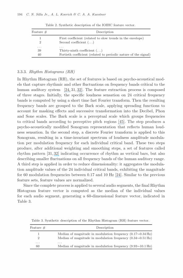
Roughly, lower coefficients represent the slowly varying trends of the envelope.It is our understanding that they encode aspects of the metrical hierarchy, theyprovide a high level view on the metrical richness, independently of the tempo.Higher coefficients, on the other hand, represent finer details of the IOIH, theyprovide a closer look at the periodic nature of this periodicity representation andare related to the pace of the piece at hand (its tempo, subdivisions and multiples),as well as to the rhythmical salience (i.e. whether the pulse is clearly established,this is reflected in the shape of the IOIH peaks: relatively high and thin peaksreflect a clear, stable pulse). More details on these features can be found in [13].Feature values are normalized to the [0, 1] interval. The overall procedure generatesa 40-dimensional feature vector that is employed for classification, illustrated inTable 2.

September 8, 2009 15:42 WSPC/214-IJSC - SPI-J091 00071

194 C. N. Silla Jr., A. L. Koerich & C. A. A. Kaestner

Table 2. Synthetic description of the IOIHC feature vector.

Feature # Description

1 First coefficient (related to slow trends in the envelope)2 Second coefficient (. . .)

. . . . . .39 Thirty-ninth coefficient (. . .)40 Fortieth coefficient (related to periodic nature of the signal)

3.3.3. Rhythm Histograms (RH)

In Rhythm Histogram (RH), the set of features is based on psycho-acoustical mod-els that capture rhythmic and other fluctuations on frequency bands critical to thehuman auditory system [24, 31, 32]. The feature extraction process is composedof three stages. Initially, the specific loudness sensation on 24 critical frequencybands is computed by using a short time fast Fourier transform. Then the resultingfrequency bands are grouped to the Bark scale, applying spreading functions toaccount for masking effects and successive transformation into the Decibel, Phonand Sone scales. The Bark scale is a perceptual scale which groups frequenciesto critical bands according to perceptive pitch regions [45]. The step produces apsycho-acoustically modified Sonogram representation that reflects human loud-ness sensation. In the second step, a discrete Fourier transform is applied to thisSonogram, resulting in a time-invariant spectrum of loudness amplitude modula-tion per modulation frequency for each individual critical band. These two stepsproduce, after additional weighting and smoothing steps, a set of features calledrhythm pattern [31, 32] indicating occurrence of rhythm as vertical bars, but alsodescribing smaller fluctuations on all frequency bands of the human auditory range.A third step is applied in order to reduce dimensionality: it aggregates the modula-tion amplitude values of the 24 individual critical bands, exhibiting the magnitudefor 60 modulation frequencies between 0.17 and 10 Hz [24]. Similar to the previousfeature sets, feature values are normalized.

Since the complete process is applied to several audio segments, the final RhythmHistogram feature vector is computed as the median of the individual valuesfor each audio segment, generating a 60-dimensional feature vector, indicated inTable 3.

Table 3. Synthetic description of the Rhythm Histogram (RH) feature vector.

Feature # Description

1 Median of magnitude in modulation frequency (0.17∼0.34 Hz)2 Median of magnitude in modulation frequency (0.34∼0.51 Hz)

. . . . . .60 Median of magnitude in modulation frequency (9.93∼10.1 Hz)

September 8, 2009 15:42 WSPC/214-IJSC - SPI-J091 00071

A Feature Selection Approach for Automatic Music Genre Classification 195

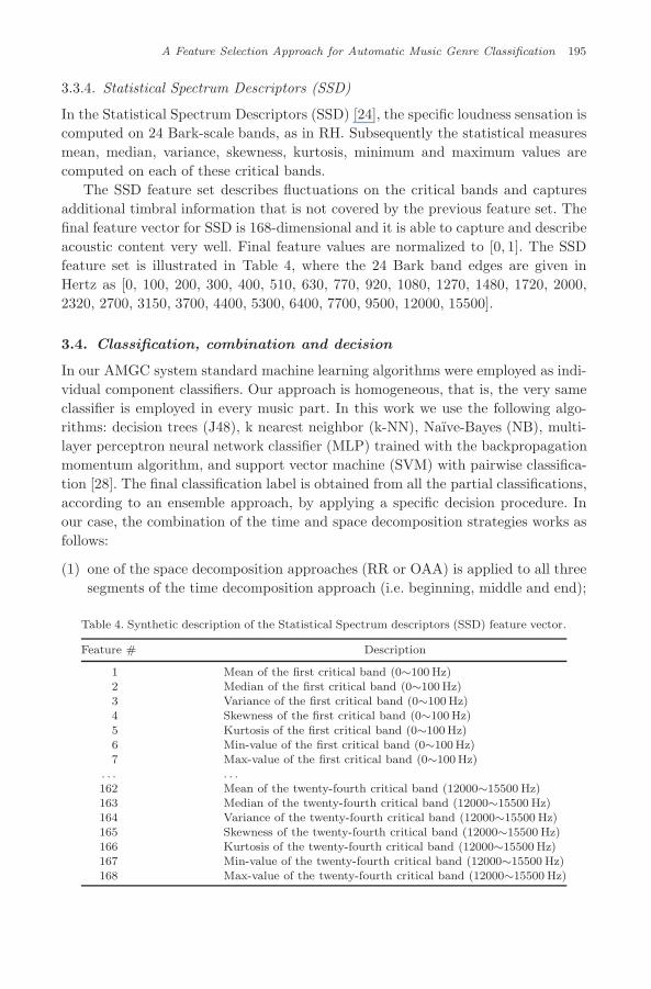
3.3.4. Statistical Spectrum Descriptors (SSD)

In the Statistical Spectrum Descriptors (SSD) [24], the specific loudness sensation iscomputed on 24 Bark-scale bands, as in RH. Subsequently the statistical measuresmean, median, variance, skewness, kurtosis, minimum and maximum values arecomputed on each of these critical bands.

The SSD feature set describes fluctuations on the critical bands and capturesadditional timbral information that is not covered by the previous feature set. Thefinal feature vector for SSD is 168-dimensional and it is able to capture and describeacoustic content very well. Final feature values are normalized to [0, 1]. The SSDfeature set is illustrated in Table 4, where the 24 Bark band edges are given inHertz as [0, 100, 200, 300, 400, 510, 630, 770, 920, 1080, 1270, 1480, 1720, 2000,2320, 2700, 3150, 3700, 4400, 5300, 6400, 7700, 9500, 12000, 15500].

3.4. Classification, combination and decision

In our AMGC system standard machine learning algorithms were employed as indi-vidual component classifiers. Our approach is homogeneous, that is, the very sameclassifier is employed in every music part. In this work we use the following algo-rithms: decision trees (J48), k nearest neighbor (k-NN), Naıve-Bayes (NB), multi-layer perceptron neural network classifier (MLP) trained with the backpropagationmomentum algorithm, and support vector machine (SVM) with pairwise classifica-tion [28]. The final classification label is obtained from all the partial classifications,according to an ensemble approach, by applying a specific decision procedure. Inour case, the combination of the time and space decomposition strategies works asfollows:

(1) one of the space decomposition approaches (RR or OAA) is applied to all threesegments of the time decomposition approach (i.e. beginning, middle and end);

Table 4. Synthetic description of the Statistical Spectrum descriptors (SSD) feature vector.

Feature # Description

1 Mean of the first critical band (0∼100 Hz)2 Median of the first critical band (0∼100 Hz)3 Variance of the first critical band (0∼100 Hz)4 Skewness of the first critical band (0∼100 Hz)

5 Kurtosis of the first critical band (0∼100 Hz)6 Min-value of the first critical band (0∼100 Hz)7 Max-value of the first critical band (0∼100 Hz)

. . . . . .162 Mean of the twenty-fourth critical band (12000∼15500 Hz)163 Median of the twenty-fourth critical band (12000∼15500 Hz)164 Variance of the twenty-fourth critical band (12000∼15500 Hz)165 Skewness of the twenty-fourth critical band (12000∼15500 Hz)166 Kurtosis of the twenty-fourth critical band (12000∼15500 Hz)167 Min-value of the twenty-fourth critical band (12000∼15500 Hz)168 Max-value of the twenty-fourth critical band (12000∼15500 Hz)

September 8, 2009 15:42 WSPC/214-IJSC - SPI-J091 00071

196 C. N. Silla Jr., A. L. Koerich & C. A. A. Kaestner

(2) a local decision considering the class of the individual segment is made basedon the underlying space decomposition approach: the majority vote for the RRand rules based on the a posteriori probability given by the specific classifier ofeach case for the OAA;

(3) the decision concerning the final music genre of the music piece is made basedon the majority vote of the predicted genres from the three individual timesegments.

Majority vote is a simple decision rule, only the class labels are taken intoaccount and the one with more votes wins

ω = maxcounti∈[1,3]

[arg max

ωj∈ΩPDi(ωj |x(i))

](8)

where i denotes the index of the segment, feature vector, and classifier and PDi

denotes the a posteriori probability provided at the output of classifier Di. Weassume that maxcount returns the most frequent value of a multiset.

4. Feature Selection

The feature selection (FS) task is defined as the choice of an adequate subset oforiginal feature set with the aim of simplifying or reducing the effort in the furthersteps, such as preprocessing and classification, while maintaining or even improvingthe final classification accuracy [3, 6]. In the case of the AMGC problem, featureselection is an important implementation issue, since computing acoustic featuresfrom a long time-varying signal is a time-consuming task.

Feature selection methods are often classified into two groups: the filter approachand the wrapper approach [29]. In the filter approach the feature selection pro-cess is carried out independently, as a preprocessing step, before the use of anymachine learning algorithm. In the wrapper approach a machine learning algorithmis employed as a sub-routine of the system, with the aim of evaluating the gener-ated solutions. In both cases the FS task can be modeled as an heuristic search:one must found a minimum size feature set that maintains or improves the musicgenre classification performance.

We emphasize that our system deals with several feature vectors, according totime and space decompositions. Therefore, the FS procedure is employed indepen-dently in the feature vectors extracted from all music segments, allowing us tocompare the relative importance of the features according to the part of the musicsignal from where they were extracted.

The proposed approach for feature selection is based on the genetic algorithmparadigm, which recognized as an efficient search procedure for complex problems.Our procedure follows a standard GA paradigm [28].

Individuals (chromosomes) are n-dimensional binary vectors, where n is themaximum size for the feature vector (30 for MARSYAS, 40 for IOIHC, 60 for RHand 168 for SSD). They work as a binary mask, acting on the original feature

September 8, 2009 15:42 WSPC/214-IJSC - SPI-J091 00071

A Feature Selection Approach for Automatic Music Genre Classification 197

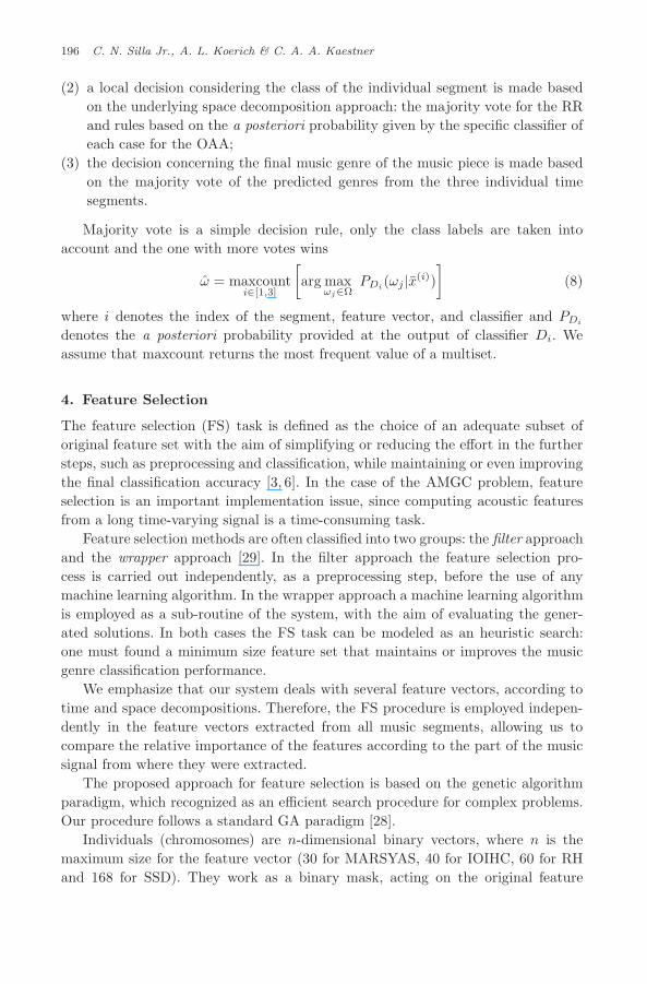
Fig. 5. The feature selection procedure for one individual in the GA procedure.

vector in order to generate the reduced final vector, composed only by the selectedfeatures, as shown in Fig. 5. Fitness of the individuals are directly obtained fromthe classification accuracy of the corresponding classifier, according to the wrapperapproach.

The global feature selection procedure is as follows:

(1) each individual works as a binary mask for an associated feature vector: a value 1indicates that the corresponding feature is used, 0 that it must be discarded;

(2) initial assignments of 0’s and 1’s are randomly generated to create initial masks;(3) a classifier is trained, for each individual, using the selected features;(4) the generated classification structure — for each individual — is applied to a

validation set to determine its accuracy, which is considered as the fitness valueof this individual;

(5) we proceed elitism to conserve the top ranked individuals; crossover and muta-tion operators are applied in order to obtain the next generation.

In our FS procedure we employ 50 individuals in each generation, and the evo-lution process ends when it converges, that is, there is no significant change in thepopulation in the successive generations, or when a fixed maximum number of gen-erations is achieved. The top ranked individual — the one associated to the highestaccuracy in the final generation — indicates the selected feature set.

5. Experiments

This section presents the experiments and the results achieved on music genre clas-sification and feature selection. The main goal of the experiments is to evaluate ifthe features extracted from different parts of the music signal have similar discrimi-native power for music genre classification. Another goal is to verify if the ensemble-based method provides better results than the classifiers taking into account featuresextracted from single segments.

Our primary evaluation measure is the classification accuracy. Experiments werecarried out using a ten-fold cross-validation procedure, that is, the presented resultsare obtained from ten randomly independent experiment repetitions.

September 8, 2009 15:42 WSPC/214-IJSC - SPI-J091 00071

198 C. N. Silla Jr., A. L. Koerich & C. A. A. Kaestner

Two databases were employed in the experiments: the Latin Music Database(LMD) and the ISMIR’2004 database. The LMD is a proprietary database com-posed of 3,227 music samples in MP3 format originated from music pieces of 501artists [37, 38]. Three thousand music samples from ten different Latin musicalgenres (Tango, Salsa, Forro, Axe, Bachata, Bolero, Merengue, Gaucha, Sertaneja,Pagode). The feature vectors from this database are available to researchers in thewebpage www.ppgia.pucpr.br/∼silla/lmd/. In this database music genre assignmentwas manually made by a group of human experts, based on the human perceptionon how each music is danced. The genre labeling was performed by two professionalteachers with over ten years of experience in teaching ballroom Latin and Braziliandances. The experiments were carried out on stratified training, validation and testdatasets. In order to deal with balanced classes, 300 different song tracks from eachgenre were randomly selected.

The ISMIR’2004 genre database is a well-known benchmark collection that wascreated for the music genre classification task of the ISMIR 2004 Audio Descriptioncontest [4, 15]. Since then, it has been used by the Music IR community. It con-tains 1,458 music pieces categorized into six popular western music genres: classical(604 pieces), electronic (229), jazz and blues (52), metal and punk (90) and worldmusic (244).

5.1. Experiments with MARSYAS features

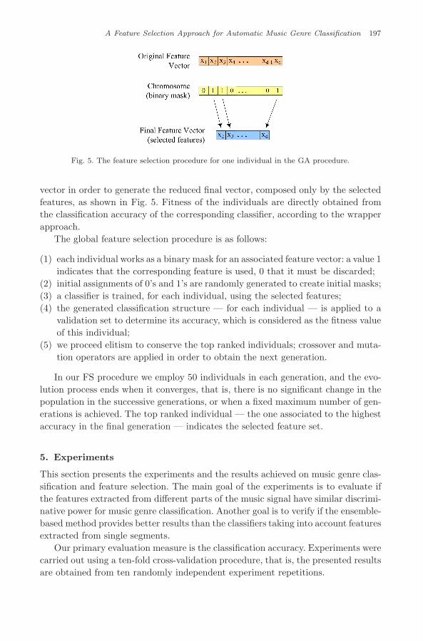
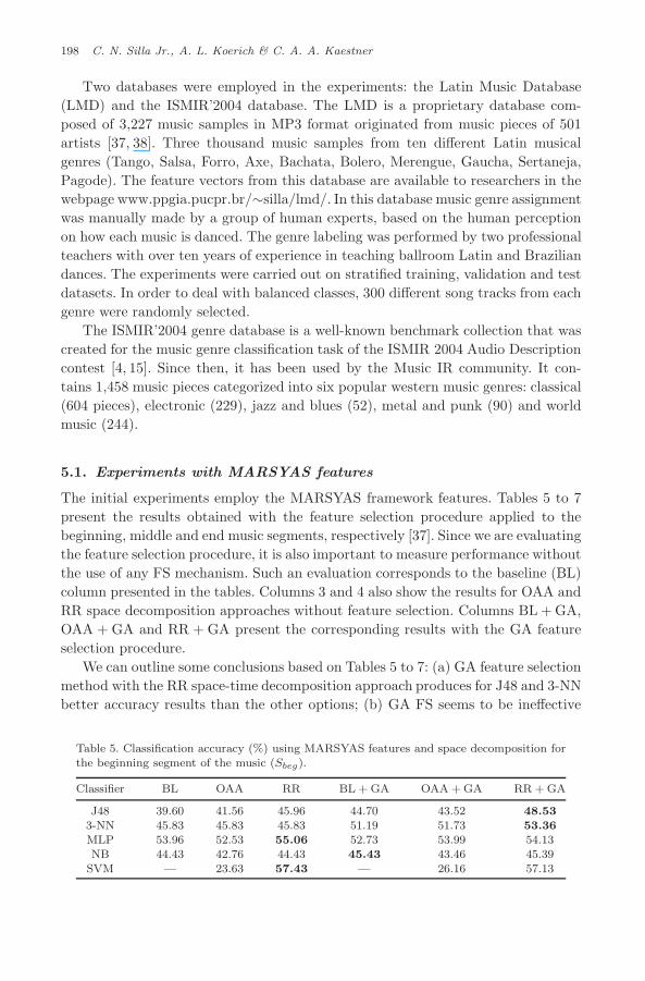
The initial experiments employ the MARSYAS framework features. Tables 5 to 7present the results obtained with the feature selection procedure applied to thebeginning, middle and end music segments, respectively [37]. Since we are evaluatingthe feature selection procedure, it is also important to measure performance withoutthe use of any FS mechanism. Such an evaluation corresponds to the baseline (BL)column presented in the tables. Columns 3 and 4 also show the results for OAA andRR space decomposition approaches without feature selection. Columns BL + GA,OAA + GA and RR + GA present the corresponding results with the GA featureselection procedure.

We can outline some conclusions based on Tables 5 to 7: (a) GA feature selectionmethod with the RR space-time decomposition approach produces for J48 and 3-NNbetter accuracy results than the other options; (b) GA FS seems to be ineffective

Table 5. Classification accuracy (%) using MARSYAS features and space decomposition forthe beginning segment of the music (Sbeg).

Classifier BL OAA RR BL + GA OAA + GA RR + GA

J48 39.60 41.56 45.96 44.70 43.52 48.533-NN 45.83 45.83 45.83 51.19 51.73 53.36MLP 53.96 52.53 55.06 52.73 53.99 54.13NB 44.43 42.76 44.43 45.43 43.46 45.39

SVM — 23.63 57.43 — 26.16 57.13

September 8, 2009 15:42 WSPC/214-IJSC - SPI-J091 00071

A Feature Selection Approach for Automatic Music Genre Classification 199

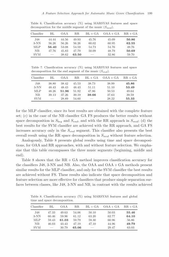
Table 6. Classification accuracy (%) using MARSYAS features and spacedecomposition for the middle segment of the music (Smid).

Classifier BL OAA RR BL + GA OAA + GA RR + GA

J48 44.44 44.56 49.93 45.76 45.09 50.863-NN 56.26 56.26 56.26 60.02 60.95 62.55MLP 56.40 53.08 54.59 54.73 54.76 49.76NB 47.76 45.83 47.79 50.09 48.79 50.69

SVM — 38.62 63.50 — 32.86 59.70

Table 7. Classification accuracy (%) using MARSYAS features and spacedecomposition for the end segment of the music (Send).

Classifier BL OAA RR BL + GA OAA + GA RR + GA

J48 38.80 38.42 45.53 38.73 38.99 45.86

3-NN 48.43 48.43 48.43 51.11 51.10 53.49MLP 48.26 51.96 51.92 47.86 50.53 49.64NB 39.13 37.26 39.19 39.66 37.63 39.59

SVM — 28.89 54.60 — 28.22 55.33

for the MLP classifier, since its best results are obtained with the complete featureset; (c) in the case of the NB classifier GA FS produces the better results withoutspace decomposition in Sbeg and Send, and with the RR approach in Smid; (d) thebest results for the SVM classifier are achieved with the RR approach, and GA FSincreases accuracy only in the Send segment. This classifier also presents the bestoverall result using the RR space decomposition in Smid without feature selection.

Analogously, Table 8 presents global results using time and space decomposi-tions, for OAA and RR approaches, with and without feature selection. We empha-size that this table encompasses the three music segments (beginning, middle andend).

Table 8 shows that the RR + GA method improves classification accuracy forthe classifiers J48, 3-NN and NB. Also, the OAA and OAA + GA methods presentsimilar results for the MLP classifier, and only for the SVM classifier the best resultsare achieved without FS. These results also indicate that space decomposition andfeature selection are more effective for classifiers that produce simple separation sur-faces between classes, like J48, 3-NN and NB, in contrast with the results achieved

Table 8. Classification accuracy (%) using MARSYAS features and globaltime and space decomposition.

Classifier BL OAA RR BL + GA OAA + GA RR + GA

J48 47.33 49.63 54.06 50.10 50.03 55.463-NN 60.46 59.96 61.12 63.20 62.77 64.10MLP 59.43 61.03 59.79 59.30 60.96 56.86NB 46.03 43.43 47.19 47.10 44.96 49.79

SVM — 30.79 65.06 — 29.47 63.03

September 8, 2009 15:42 WSPC/214-IJSC - SPI-J091 00071

200 C. N. Silla Jr., A. L. Koerich & C. A. A. Kaestner

with the MLP and SVM classifiers, which can produce complex separation surfaces.This situation corroborates to our hypothesis on the use of space decompositionstrategies.

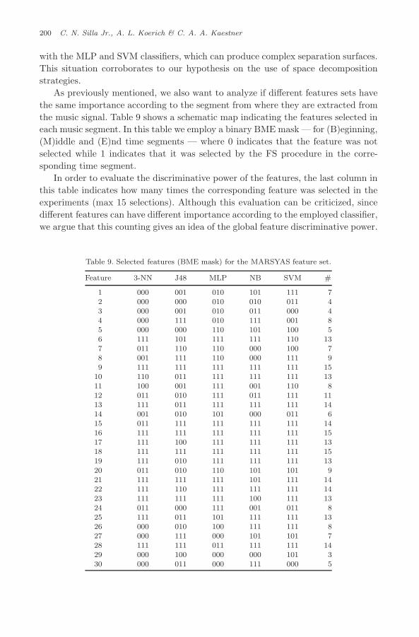
As previously mentioned, we also want to analyze if different features sets havethe same importance according to the segment from where they are extracted fromthe music signal. Table 9 shows a schematic map indicating the features selected ineach music segment. In this table we employ a binary BME mask — for (B)eginning,(M)iddle and (E)nd time segments — where 0 indicates that the feature was notselected while 1 indicates that it was selected by the FS procedure in the corre-sponding time segment.

In order to evaluate the discriminative power of the features, the last column inthis table indicates how many times the corresponding feature was selected in theexperiments (max 15 selections). Although this evaluation can be criticized, sincedifferent features can have different importance according to the employed classifier,we argue that this counting gives an idea of the global feature discriminative power.

Table 9. Selected features (BME mask) for the MARSYAS feature set.

Feature 3-NN J48 MLP NB SVM #

1 000 001 010 101 111 72 000 000 010 010 011 43 000 001 010 011 000 44 000 111 010 111 001 85 000 000 110 101 100 56 111 101 111 111 110 137 011 110 110 000 100 78 001 111 110 000 111 99 111 111 111 111 111 15

10 110 011 111 111 111 1311 100 001 111 001 110 812 011 010 111 011 111 1113 111 011 111 111 111 1414 001 010 101 000 011 615 011 111 111 111 111 1416 111 111 111 111 111 1517 111 100 111 111 111 1318 111 111 111 111 111 1519 111 010 111 111 111 13

20 011 010 110 101 101 921 111 111 111 101 111 1422 111 110 111 111 111 1423 111 111 111 100 111 1324 011 000 111 001 011 825 111 011 101 111 111 1326 000 010 100 111 111 827 000 111 000 101 101 728 111 111 011 111 111 1429 000 100 000 000 101 330 000 011 000 111 000 5

September 8, 2009 15:42 WSPC/214-IJSC - SPI-J091 00071

A Feature Selection Approach for Automatic Music Genre Classification 201

For example, features 6, 9, 10, 13, 15, 16, 17, 18, 19, 21, 22, 23, 25 and 28 areimportant for music genre classification. We remember that features 1 to 6 are beatrelated, 7 to 25 are related to timbral texture, and 26 to 30 are pitch related.

5.2. Experiments with other feature sets

We also conduct some experiments using the alternative feature sets described inSecs. 3.3.2 to 3.3.4. Since the SVM classifier presents the best results in the previousexperiments, we have limited the further experiments to this specific classifier.

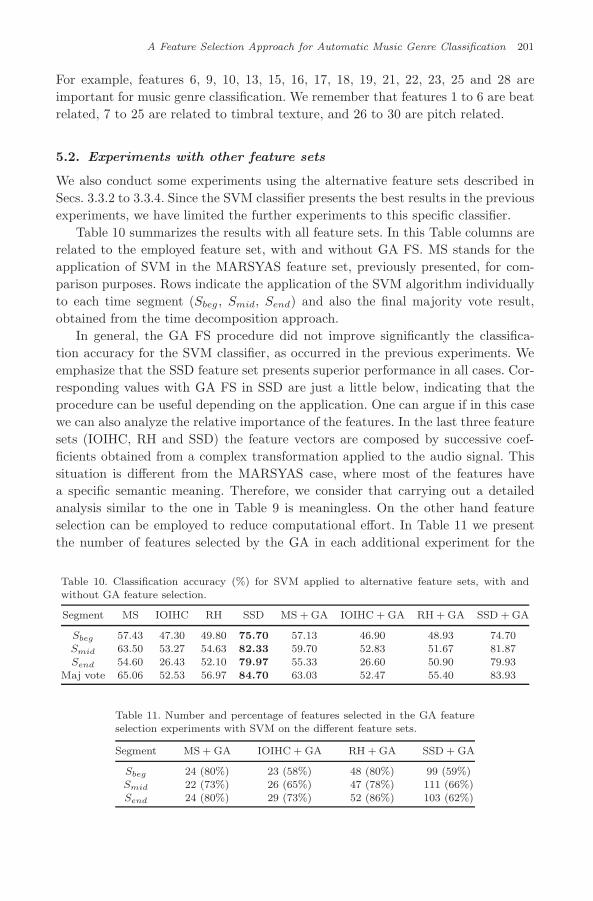
Table 10 summarizes the results with all feature sets. In this Table columns arerelated to the employed feature set, with and without GA FS. MS stands for theapplication of SVM in the MARSYAS feature set, previously presented, for com-parison purposes. Rows indicate the application of the SVM algorithm individuallyto each time segment (Sbeg , Smid, Send) and also the final majority vote result,obtained from the time decomposition approach.

In general, the GA FS procedure did not improve significantly the classifica-tion accuracy for the SVM classifier, as occurred in the previous experiments. Weemphasize that the SSD feature set presents superior performance in all cases. Cor-responding values with GA FS in SSD are just a little below, indicating that theprocedure can be useful depending on the application. One can argue if in this casewe can also analyze the relative importance of the features. In the last three featuresets (IOIHC, RH and SSD) the feature vectors are composed by successive coef-ficients obtained from a complex transformation applied to the audio signal. Thissituation is different from the MARSYAS case, where most of the features havea specific semantic meaning. Therefore, we consider that carrying out a detailedanalysis similar to the one in Table 9 is meaningless. On the other hand featureselection can be employed to reduce computational effort. In Table 11 we presentthe number of features selected by the GA in each additional experiment for the

Table 10. Classification accuracy (%) for SVM applied to alternative feature sets, with andwithout GA feature selection.

Segment MS IOIHC RH SSD MS + GA IOIHC + GA RH + GA SSD + GA

Sbeg 57.43 47.30 49.80 75.70 57.13 46.90 48.93 74.70Smid 63.50 53.27 54.63 82.33 59.70 52.83 51.67 81.87Send 54.60 26.43 52.10 79.97 55.33 26.60 50.90 79.93

Maj vote 65.06 52.53 56.97 84.70 63.03 52.47 55.40 83.93

Table 11. Number and percentage of features selected in the GA featureselection experiments with SVM on the different feature sets.

Segment MS + GA IOIHC + GA RH + GA SSD + GA

Sbeg 24 (80%) 23 (58%) 48 (80%) 99 (59%)Smid 22 (73%) 26 (65%) 47 (78%) 111 (66%)Send 24 (80%) 29 (73%) 52 (86%) 103 (62%)

September 8, 2009 15:42 WSPC/214-IJSC - SPI-J091 00071

202 C. N. Silla Jr., A. L. Koerich & C. A. A. Kaestner

different feature sets. Recall that the original feature set sizes are 30, 40, 60, and168 for MARSYAS, IOIHC, RH and SSD respectively.

Overall, we note that from 58% to 86% of the features were selected. In theMARSYAS and RH feature sets the average percentual of features selected isroughly 80%. In the SSD feature set which, is the one with the highest dimen-sion, on average only 62% of the features were selected. This reduction can beuseful in practical applications, especially if we consider that the corresponding fallin accuracy (Table 10) is less than 1%.

5.3. Experiments with PCA feature construction

We conduct experiments in order to compare our FS approach based on GA withthe well-known PCA feature construction procedure that is used by several authorsfor FS [9–11, 44]. As in the previous section, we restrict our analysis to the SVMclassifier, and we use the WEKA data mining tool with standard parameters in theexperiments, i.e. the new features account for 95% of the variance of the originalfeatures.

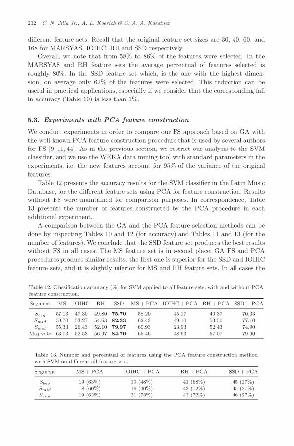
Table 12 presents the accuracy results for the SVM classifier in the Latin MusicDatabase, for the different feature sets using PCA for feature construction. Resultswithout FS were maintained for comparison purposes. In correspondence, Table13 presents the number of features constructed by the PCA procedure in eachadditional experiment.

A comparison between the GA and the PCA feature selection methods can bedone by inspecting Tables 10 and 12 (for accuracy) and Tables 11 and 13 (for thenumber of features). We conclude that the SSD feature set produces the best resultswithout FS in all cases. The MS feature set is in second place. GA FS and PCAprocedures produce similar results: the first one is superior for the SSD and IOIHCfeature sets, and it is slightly inferior for MS and RH feature sets. In all cases the

Table 12. Classification accuracy (%) for SVM applied to all feature sets, with and without PCAfeature construction.

Segment MS IOIHC RH SSD MS + PCA IOIHC + PCA RH + PCA SSD + PCA

Sbeg 57.13 47.30 49.80 75.70 58.20 45.17 49.37 70.33Smid 59.70 53.27 54.63 82.33 62.43 49.10 53.50 77.10Send 55,33 26.43 52.10 79.97 60.93 23.93 52.43 74.90

Maj vote 63.03 52.53 56.97 84.70 65.46 48.63 57.07 79.90

Table 13. Number and percentual of features using the PCA feature construction methodwith SVM on different all feature sets.

Segment MS + PCA IOIHC + PCA RH + PCA SSD + PCA

Sbeg 19 (63%) 19 (48%) 41 (68%) 45 (27%)Smid 18 (60%) 16 (40%) 43 (72%) 45 (27%)Send 19 (63%) 31 (78%) 43 (72%) 46 (27%)

September 8, 2009 15:42 WSPC/214-IJSC - SPI-J091 00071

A Feature Selection Approach for Automatic Music Genre Classification 203

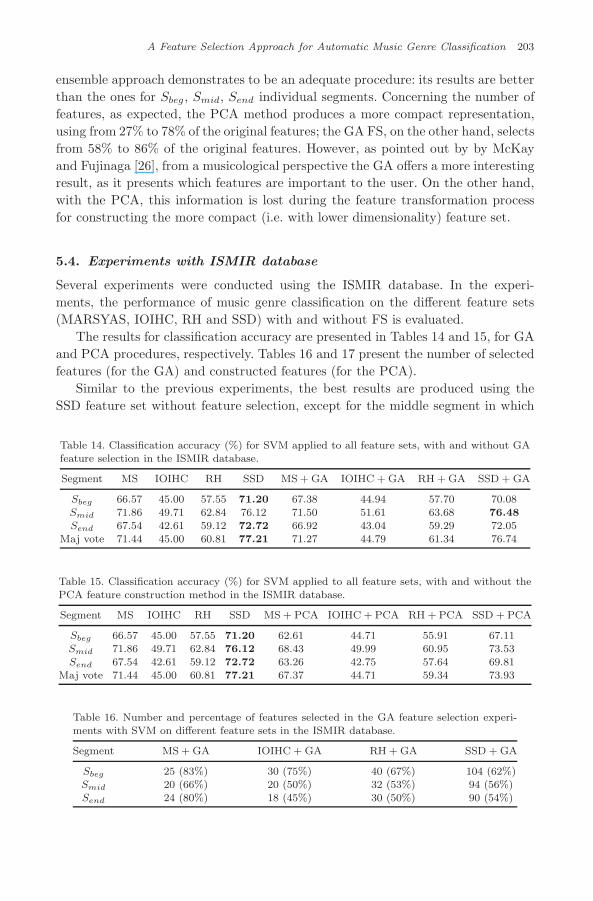
ensemble approach demonstrates to be an adequate procedure: its results are betterthan the ones for Sbeg, Smid, Send individual segments. Concerning the number offeatures, as expected, the PCA method produces a more compact representation,using from 27% to 78% of the original features; the GA FS, on the other hand, selectsfrom 58% to 86% of the original features. However, as pointed out by by McKayand Fujinaga [26], from a musicological perspective the GA offers a more interestingresult, as it presents which features are important to the user. On the other hand,with the PCA, this information is lost during the feature transformation processfor constructing the more compact (i.e. with lower dimensionality) feature set.

5.4. Experiments with ISMIR database

Several experiments were conducted using the ISMIR database. In the experi-ments, the performance of music genre classification on the different feature sets(MARSYAS, IOIHC, RH and SSD) with and without FS is evaluated.

The results for classification accuracy are presented in Tables 14 and 15, for GAand PCA procedures, respectively. Tables 16 and 17 present the number of selectedfeatures (for the GA) and constructed features (for the PCA).

Similar to the previous experiments, the best results are produced using theSSD feature set without feature selection, except for the middle segment in which

Table 14. Classification accuracy (%) for SVM applied to all feature sets, with and without GAfeature selection in the ISMIR database.

Segment MS IOIHC RH SSD MS + GA IOIHC + GA RH + GA SSD + GA

Sbeg 66.57 45.00 57.55 71.20 67.38 44.94 57.70 70.08Smid 71.86 49.71 62.84 76.12 71.50 51.61 63.68 76.48Send 67.54 42.61 59.12 72.72 66.92 43.04 59.29 72.05

Maj vote 71.44 45.00 60.81 77.21 71.27 44.79 61.34 76.74

Table 15. Classification accuracy (%) for SVM applied to all feature sets, with and without thePCA feature construction method in the ISMIR database.

Segment MS IOIHC RH SSD MS + PCA IOIHC + PCA RH + PCA SSD + PCA

Sbeg 66.57 45.00 57.55 71.20 62.61 44.71 55.91 67.11Smid 71.86 49.71 62.84 76.12 68.43 49.99 60.95 73.53Send 67.54 42.61 59.12 72.72 63.26 42.75 57.64 69.81

Maj vote 71.44 45.00 60.81 77.21 67.37 44.71 59.34 73.93

Table 16. Number and percentage of features selected in the GA feature selection experi-ments with SVM on different feature sets in the ISMIR database.

Segment MS + GA IOIHC + GA RH + GA SSD + GA

Sbeg 25 (83%) 30 (75%) 40 (67%) 104 (62%)Smid 20 (66%) 20 (50%) 32 (53%) 94 (56%)Send 24 (80%) 18 (45%) 30 (50%) 90 (54%)

September 8, 2009 15:42 WSPC/214-IJSC - SPI-J091 00071

204 C. N. Silla Jr., A. L. Koerich & C. A. A. Kaestner

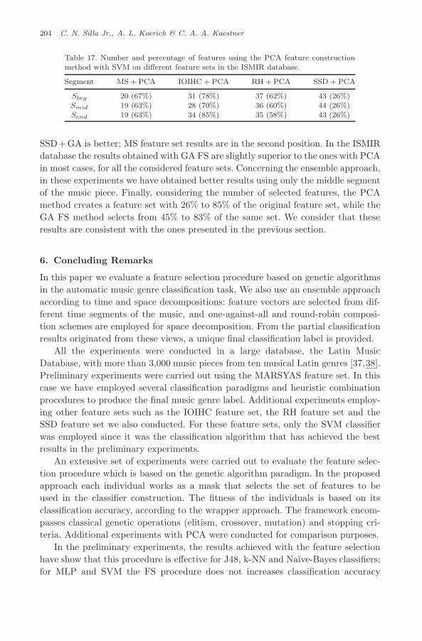
Table 17. Number and percentage of features using the PCA feature constructionmethod with SVM on different feature sets in the ISMIR database.

Segment MS + PCA IOIHC + PCA RH + PCA SSD + PCA

Sbeg 20 (67%) 31 (78%) 37 (62%) 43 (26%)Smid 19 (63%) 28 (70%) 36 (60%) 44 (26%)Send 19 (63%) 34 (85%) 35 (58%) 43 (26%)

SSD+GA is better; MS feature set results are in the second position. In the ISMIRdatabase the results obtained with GA FS are slightly superior to the ones with PCAin most cases, for all the considered feature sets. Concerning the ensemble approach,in these experiments we have obtained better results using only the middle segmentof the music piece. Finally, considering the number of selected features, the PCAmethod creates a feature set with 26% to 85% of the original feature set, while theGA FS method selects from 45% to 83% of the same set. We consider that theseresults are consistent with the ones presented in the previous section.

6. Concluding Remarks

In this paper we evaluate a feature selection procedure based on genetic algorithmsin the automatic music genre classification task. We also use an ensemble approachaccording to time and space decompositions: feature vectors are selected from dif-ferent time segments of the music, and one-against-all and round-robin composi-tion schemes are employed for space decomposition. From the partial classificationresults originated from these views, a unique final classification label is provided.

All the experiments were conducted in a large database, the Latin MusicDatabase, with more than 3,000 music pieces from ten musical Latin genres [37,38].Preliminary experiments were carried out using the MARSYAS feature set. In thiscase we have employed several classification paradigms and heuristic combinationprocedures to produce the final music genre label. Additional experiments employ-ing other feature sets such as the IOIHC feature set, the RH feature set and theSSD feature set we also conducted. For these feature sets, only the SVM classifierwas employed since it was the classification algorithm that has achieved the bestresults in the preliminary experiments.

An extensive set of experiments were carried out to evaluate the feature selec-tion procedure which is based on the genetic algorithm paradigm. In the proposedapproach each individual works as a mask that selects the set of features to beused in the classifier construction. The fitness of the individuals is based on itsclassification accuracy, according to the wrapper approach. The framework encom-passes classical genetic operations (elitism, crossover, mutation) and stopping cri-teria. Additional experiments with PCA were conducted for comparison purposes.

In the preliminary experiments, the results achieved with the feature selectionhave show that this procedure is effective for J48, k-NN and Naıve-Bayes classifiers;for MLP and SVM the FS procedure does not increases classification accuracy

September 8, 2009 15:42 WSPC/214-IJSC - SPI-J091 00071

A Feature Selection Approach for Automatic Music Genre Classification 205

(Tables 5 to 8). These results are compatible with the ones presented in [44]. Thisconclusion is also confirmed in the experiments carried out using three differentfeature sets. In this case, the SSD feature set, composed by a series of statisticaldescriptors of the signal spectrum, was the feature set that has presented by far thebest results in terms of accuracy. We also conduct experiments using the ISMIR 2004Audio Description contest dataset. The results of these experiments are, in general,consistent with those obtained with the LMD database (see Tables 14 to 17).

Another conclusion that can inferred from the initial experiments is that theMARSYAS features have different importance in the classification, according totheir origin music segment (Table 9). It can be seen, however, that some features arepresent in almost every selection, showing they have a strong discriminative power inthe classification task. In the case of the alternative feature sets (IOIHC, RH, SSD)the feature selection procedure did not increase the classification accuracy (Tables 10to 11). We argue that this occurs because these feature sets are composed of a seriesof coefficients obtained from an unique signal representation, as shown in Tables 2to 4. Therefore, it is expected that all the features have a similar discriminativepower.

We emphasize that the use of the time/space decomposition approach representsan interesting trade-off between classification accuracy and computational effort;also, the use of a reduced set of features implies a smaller processing time. Thispoint is an important issue in practical applications, where an adequate compromisebetween the quality of a solution and the time to obtain it must be achieved. Indeed,the most adequate feature set, the music signal segment from where the featuresare extracted, the number and the duration of the time segments, the use of spacedecomposition strategies and the discovery of the more discriminative features stillremain open questions for the automatic music genre classification problem.

Acknowledgments

The authors would like to thank CAPES — a Brazilian research-support agency(process number 4871-06-5) and Mr. Breno Moiana for his invaluable help with theexperiment infrastructure. We would also like to thank Dr. George Tzanetakis, Dr.Fabien Gouyon and Mr. Thomas Lidy for providing the feature extraction algo-rithms used in this work.

References

[1] J. J. Aucouturier and F. Pachet, Representing musical genre: A state of the art,Journal of New Music Research 32 (2003) 83–93.

[2] J. Bergstra, N. Casagrande, D. Erhan, D. Eck and B. Kegl, Aggregate features andADABOOST for music classification, Machine Learning 65(2–3) (2006) 473–484.

[3] A. Blum and P. Langley, Selection of relevant features and examples in machinelearning, Artificial Intelligence 97 (1997) 245–271.

September 8, 2009 15:42 WSPC/214-IJSC - SPI-J091 00071

206 C. N. Silla Jr., A. L. Koerich & C. A. A. Kaestner

[4] P. Cano, E. Gomez, F. Gouyon, P. Herrera, M. Koppenberger B. Ong, X. Serra,S. Streich and N. Wack, ISMIR 2004 Audio Description Contest, Technical ReportMTG-TR-2006-02, Music Technology Group, Pompeu Fabra University, 2006.

[5] C. H. L. Costa, J. D. Valle Jr. and A. L. Koerich, Automatic Classification of AudioData, in Proc. of the IEEE Int. Conf. on Systems, Man, and Cybernetics, The Hague,Holland, 2004, pp. 562–567.

[6] M. Dash and H. Liu, Feature selection for classification, Intelligent Data Analysis 1(1997) 131–156.

[7] T. G. Dietterich, Ensemble methods in Machine Learning, in Proc. of the 1st Int.Workshop on Multiple Classifier System, Lecture Notes in Computer Science 1857,2000, pp. 1–15.

[8] J. S. Downie and S. J. Cunningham, Toward a theory of music information retrievalqueries: System design implications, in Proc. of the 3rd Int. Conf. on Music Infor-mation Retrieval, Paris, France, 2002, pp. 299–300.

[9] R. Fiebrink and I. Fujinaga, Feature Selection Pitfalls and Music Classification, inProc. of the 7th Int. Conf. on Music Information Retrieval, Victoria, CA, USA, 2006,pp. 340–341.

[10] M. Grimaldi, P. Cunningham and A. Kokaram, A Wavelet Packet representationof audio signals for music genre classification using different ensemble and featureselection techniques, in Proc. of the 5th ACM SIGMM Int. Workshop on MultimediaInformation Retrieval, Berkeley, CA, USA, 2003, pp. 102–108.

[11] M. Grimaldi, P. Cunningham and A. Kokaram, An evaluation of alternative featureselection strategies and ensemble techniques for classifying music, in Workshop onMultimedia Discovery and Mining, 14th European Conference on Machine Learn-ing, 7th European Conference on Principles and Practice of Knowledge Discovery inDatabases, Dubrovnik, Croatia, 2003.

[12] F. Gouyon, P. Herrera and P. Cano, Pulse-dependent analysis of percussive music,in Proc. of the 22th Int. AES Conference on Virtual, Synthetic and EntertainmentAudio, Espoo, Finland, 2002.

[13] F. Gouyon, S. Dixon, E. Pampalk and G. Widmer, Evaluating rhytmic descriptionsfor music genre classification, in Proc. of the 25th Int. AES Conference on Virtual,Synthetic and Entertainment Audio, London, UK, 2004.

[14] S. Hacker, MP3: The Definitive Guide (O’Reilly Publishers, 2000).[15] Audio Description Contest, Website, URL http://ismir2004.ismir.net/ISMIR

Contest.html, 2004.[16] J. Kittler, M. Hatef, R. P. W. Duin and J. Matas, On combining classifiers, IEEE

Transactions on Pattern Analysis and Machine Intelligence 20(3) (1998) 226–239.[17] K. Kosina, Music Genre Recognition, MSc. dissertation, Fachschule Hagenberg, June

2002.[18] J. H. Lee and J. S. Downie, Survey of music information needs, uses, and seeking

behaviours: preliminary findings, in Proc. of the 5th Int. Conf. on Music InformationRetrieval, Barcelona, Spain, 2004, pp. 441–446.

[19] Magnatune, “Magnatune: MP3 Music and Music Licensing (Royalty Free Music andLicense Music),” [Web site] 2006, Available: http://www.magnatune.com

[20] D. McEnnis, C. McKay, I. Fujinaga and P. Depalle, jAudio: A Feature ExtractionLibrary, in Proc. of the 6th Int. Conf. on Music Information Retrieval, London, UK,2005, pp. 600–603.

[21] M. Li and R. Sleep, Genre Classification via an LZ78-Based String Kernel, in Proc. ofthe 6th Int. Conf. on Music Information Retrieval, London, UK, 2005, pp. 252–259.

September 8, 2009 15:42 WSPC/214-IJSC - SPI-J091 00071

A Feature Selection Approach for Automatic Music Genre Classification 207

[22] T. Li, M. Ogihara and Q. Li, A Comparative study on content-based Music GenreClassification, in Proc. of the 26th Annual Int. ACM SIGIR Conference on Researchand Development in Information Retrieval, Toronto, Canada, 2003, pp. 282–289.

[23] T. Li and M. Ogihara, Music Genre Classification with Taxonomy, in Proc. of IEEEInt. Conference on Acoustics, Speech and Signal Processing, Philadelphia, PA, USA,2005, pp. 197–200.

[24] T. Lidy and A. Rauber, Evaluation of feature extractors and psycho-acoustic tranfor-mations for music genre classification, in Proc. of the 6th Int. Conference on MusicInformation Retrieval, London, UK, 2005, pp. 34–41.

[25] H. Liu and L. Yu, Feature Extraction, Selection, and Construction, in The Handbookof Data Mining, ed. Nong Ye (Lawrence Erlbaum Publishers, 2003), pp. 409–424.

[26] C. McKay and I. Fujinaga, Musical Genre Classification: Is it worth pursuing and howcan it be?, in Proc. of the 7th Int. Conf. on Music Information Retrieval, Victoria,CA, USA, 2006, pp. 101–106.

[27] A. Meng, P. Ahrendt and J. Larsen, Improving Music Genre Classification By Short-Time Feature Integration, in Proc. of the IEEE Int. Conference on Acoustics, Speech,and Signal Processing, Philadelphia, PA, USA, 2005, pp. 497–500.

[28] T. M. Mitchell, Machine Learning (McGraw-Hill, 1997).[29] L. C. Molina, L. Belanche and A. Nebot, Feature Selection Algorithms: a Survey

and experimental Evaluation, in Proc. of the IEEE Int. Conference on Data Mining,Maebashi City, JP, 2002, pp. 306–313.

[30] E. Pampalk, A. Rauber and D. Merkl, Content-based Organization and Visualiza-tion of Music Archives, in Proc.of the ACM Multimedia, Juan-les-Pins, France, 2002,pp. 570–579.

[31] A. Rauber, E. Pampalk and D. Merkl, Using Psycho-acoustic transformations formusic genre classification, in Proc. of the 3rd Int. Conference on Music InformationRetrieval, Paris, France, 2002, pp. 71–80.

[32] A. Rauber, E. Pampalk and D. Merkl, The SOM-enhanced JukeBox: organizationand visualization of music collections based on perceptual models, Journal of NewMusic Research 32(2) (2003) 193–210.

[33] D. Rocchesso, Introduction to Sound Processing, 1st ed. (Universita di Verona, 2003).[34] C. N. Silla Jr., C. A. A. Kaestner and A. L. Koerich, Time-Space Ensemble Strategies

for Automatic Music Genre Classification, in Proc. of the Brazilian Symposium onArtificial Intelligence, Ribeirao Preto, SP, Brazil, Lecture Notes in Computer Science4140, 2006, pp. 339–348.

[35] C. N. Silla Jr., C. A. A. Kaestner and A. L. Koerich, The Latin Music Database: adatabase for the automatic classification of music genres (in portuguese). Proc. of 11thBrazilian Symposium on Computer Music, Sao Paulo, SP, Brazil, 2007, pp. 167–174.

[36] C. N. Silla Jr., C. A. A. Kaestner and A. L. Koerich, Automatic Music Genre Classifi-cation using Ensemble of Classifiers, in Proc. of the IEEE Int. Conference on Systems,Man and Cybernetics, Montreal, Canada, 2007, pp. 1687–1692.

[37] C. N. Silla Jr., Classifiers Combination for Automatic Music Classification (in por-tuguese), MSc dissertation, Graduate Program in Applied Computer Science, Pontif-ical Catholic University of Parana, 2007.

[38] C. N. Silla Jr., A. L. Koerich and C. A. A. Kaestner, The Latin Music Database, inProc. of the 9th Int. Conference on Music Information Retrieval, Philadelphia, PA,USA, 2008, pp. 451–456.

[39] C. N. Silla Jr., A. L. Koerich and C. A. A. Kaestner, A machine learning approachto automatic music genre classification, Journal of the Brazilian Computer Society14(3) (2008) 7–18.

September 8, 2009 15:42 WSPC/214-IJSC - SPI-J091 00071

208 C. N. Silla Jr., A. L. Koerich & C. A. A. Kaestner

[40] C. N. Silla Jr., A. L. Koerich and C. A. A. Kaestner, Feature Selection in AutomaticMusic Genre Classification, in Proc. of the 10th Int. Symp. on Multimedia, Berkeley,CA, USA, 2008, pp. 39–44.

[41] A. Stolcke, Y. Konig and M. Weintraub, Explicit word error minimization in n-bestlist rescoring, in Proc. of Eurospeech 97, Rhodes, Greece, 1997, pp. 163–166.

[42] G. Tzanetakis and P. Cook, Musical genre classification of audio signals, IEEE Trans-actions on Speech and Audio Processing 10 (2002) 293–302.

[43] I. H. Witten and E. Frank, Data Mining: Practical Machine Learning Tools andTechniques (Morgan Kaufmann, San Francisco, 2005).

[44] Y. Yaslan and Z. Cataltepe, Audio Music Genre Classification Using Different Clas-sifiers and Feature Selection Methods, in Proc. of the Int. Conference on PatternRecognition, Hong Kong, China, 2006, pp. 573–576.

[45] E. Zicker and H. Fastl, Pcychoacoustics — Facts and Models, Springer Series onInformation Sciences 22 (Springer, Berlin, 1999).