Journal of

Marine Science and Engineering

Article

A Fast Algorithm for the Prediction of Ship-BankInteraction in Shallow Water

Jin Huang 1,2, Chen Xu 1,2, Ping Xin 1,2, Xueqian Zhou 1,2,* , Serge Sutulo 2,3

and Carlos Guedes Soares 2,3

1 College of Shipbuilding Engineering, Harbin Engineering University, Harbin 150001, China;james0451@126.com (J.H.); xuchen@hrbeu.edu.cn (C.X.); xinpingsmu@163.com (P.X.)

2 International Joint Laboratory of Naval Architecture and Offshore Technology between Harbin EngineeringUniversity and Lisbon University, Harbin 150001, China; serge.sutulo@centec.tecnico.ulisboa.pt (S.S.);c.guedes.soares@centec.tecnico.ulisboa.pt (C.G.S.)

3 Centre for Marine Technology and Ocean Engineering (CENTEC), Instituto Superior Técnico,Universidade de Lisboa, 1049-001 Lisboa, Portugal

* Correspondence: xueqian.zhou@hrbeu.edu.cn; Tel.: +86-451-82519902

Received: 1 October 2020; Accepted: 12 November 2020; Published: 16 November 2020�����������������

Abstract: The hydrodynamic interaction induced by the complex flow around a ship maneuvering inrestricted waters has a significant influence on navigation safety. In particular, when a ship moves inthe vicinity of a bank, the hydrodynamic interaction forces caused by the bank effect can significantlyaffect the ship’s maneuverability. An efficient algorithm integrated in onboard systems or simulatorsfor capturing the bank effect with fair accuracy would benefit navigation safety. In this study,an algorithm based on the potential-flow theory is presented for efficient calculation of ship-bankhydrodynamic interaction forces. Under the low Froude number assumption, the free surfaceboundary condition is approximated using the double-body model. A layer of sources is dynamicallydistributed on part of the seabed and bank in the vicinity of the ship to model the boundary conditions.The sinkage and trim are iteratively solved via hydrostatic balance, and the importance of includingsinkage and trim is investigated. To validate the numerical method, a series of simulations withvarious configurations are carried out, and the results are compared with experiment and numericalresults obtained with RANSE-based and Rankine source methods. The comparison and analysisshow the accuracy of the method proposed in this paper satisfactory except for extreme shallowwater cases.

Keywords: ship-bank hydrodynamic interaction; sinkage and trim; potential flow theory; paneledmoving patch

1. Introduction

Maneuvering of large vessels near a bank is a hot topic [1–3] and a difficult problem in ship controldue to the complex flow around the ship. Many accidents that occurred in the berthing process havebeen reported. Prediction of ship-bank interaction in restricted waters, as one of the inputs to shipberthing control system [4,5], has received significant attention in recent years [6–8].

Physically, asymmetric flow around the ship induced by the vicinity of banks causes the pressuredifference between port and starboard sides. As a result, the lateral force mostly directed to the closestbank, and the stern suction yaw moment will act on the ship. In addition, the squat phenomenon dueto the reduced pressure over the ship bottom surface increases the risk of grounding, and also affectsthe hydrodynamic performance.

Regarding the ship-bank effect, a large group of earlier researches are based on experimentationusually producing rather realistic and reliable results. One of the pioneering studies on ship-bank

J. Mar. Sci. Eng. 2020, 8, 927; doi:10.3390/jmse8110927 www.mdpi.com/journal/jmse

J. Mar. Sci. Eng. 2020, 8, 927 2 of 19

interaction was performed by Norrbin [9], who carried out a series of free-run trajectory tests withmodels moving along vertical sidewall of a dredged channel.

Lataire and Delefortrie [10] carried out a comprehensive set of ship-bank interaction model tests,and the influence of various parameters was presented, such as the ship speed, water depth, ship-bankdistance, and the bank’s profile. Based on the earlier obtained experimental data [10], Lataire andDelefortrie [11] proposed a regression model for estimating the sway force and yaw moment inducedby the bank effect on a moving ship. The model was later extended to cover the case of an arbitrarilyshaped bank [12].

Although methods based on model tests are widely used for estimating the forces caused by theship-bank interaction, they have limitations [13]: only a limited number of ship types can be used inthe experiments; the scaled models’ tests always have restrictions on the boundary profile and onthe motions of the ship model. These limitations may seriously impair applicability of the resultingmodels to, say, automated ship berthing systems. Moreover, the semi-analytical approach basedon regression model is a fast and robust way to predict ship responses under the bank effect, but asignificant number of systematic and expensive model tests are required to establish a semi-analyticalformula for ship-bank interaction.

Analysis of the ship-bank hydrodynamic interaction in restricted waters based on the slender-bodytheory and matched asymptotic expansions was presented by Beck [14]. The same approach wasalso applied for predicting hydrodynamic interaction between the ship and the pier [15]. However,applicability of this method to full-bodied ships may seem doubtful.

Rapid development of the computing hardware facilitated application of 3D numerical methodsfor potential flow and of more complex field methods for inviscid and viscous fluid typically associatedwith the Computational Fluid Dynamics (CFD). Ma et al. [16] applied CFD simulations for investigatingthe hydrodynamic interaction between the ship’s hull, rudder, and the bank for a ship moving along asloped wall. Kaidi et al. [17] also used CFD software to estimate the influence of the bank-propellereffect on the hydrodynamic forces. Simulating the ship-bank interaction with a CFD code on the basisof the Reynolds-Averaged Navier-Stokes Equations (RANSE), Zou and Larsson [6] demonstrated goodagreement with experimental data having paid special attention to analysis of the grid convergence.

Xu et al. [7] applied a NURBS-based high-order panel method to study the bank effects onthe hydrodynamic interaction between two Wigley ships encountering and overtaking in a channel.A numerical method based on the Rankine source distribution and accounting for the free-surfaceeffects was used by Yuan [18] to study the ship-bank and ship-lock interaction in restricted waterways.Comparisons with the double-body model, viscous flow computations, and model test showed thatthe free-surface effects are more important than effects of viscosity in the ship-lock problem. As for thewave effects in the problem of ship-bank interaction, the comparison in [8] showed that the influenceis not significant in a relatively large ship-bank distance and an intermediate water depth. For theextreme conditions, the variation of free surface may play an important role.

Although field methods usually produce rather accurate results and can provide useful informationabout the velocity field which is useful for understanding underlying physics, these methodsare not computationally efficient which prevents their application in real-time simulation anddecision-support systems.

A code based on the classic Hess and Smith panel method [19] was developed by Sutulo and GuedesSoares [13] and validated against experiments [20]. The free surface condition was approximated bythe double-body model under the assumption of low Froude numbers. Neglecting the free surfaceeffects significantly improved the computational efficiency, and real-time simulations of multi-bodymaneuvering were made possible. The mirror-image technique [20] and paneled moving patchmethod [21] were adopted to extend the algorithm to cover shallow water cases. The latter method canbe used for modeling vertical and sloped banks.

All numerical methods proposed to estimate the hydrodynamic interaction loads can be classifiedaccording to various aspects such as including or excluding the fluid viscosity, including or excluding

J. Mar. Sci. Eng. 2020, 8, 927 3 of 19

the free surface effect, and ability of online computations. Comparative studies have shown theimportant influence of free surface in the case of multiple ships encountering with high speed [22] andthe non-negligible viscosity effect in the extreme close maneuver situations [23]; although, in general,information obtained so far is not conclusive [24]. Additionally, the influence of fluid viscosity and ofwave-making effects on the ship-bank interaction effects was studied much less.

The squat phenomenon is common in shallow water navigation and it has been studiedexperimentally [25], by means of viscous flow simulations [26] as well as with the potential flowtheory [27]. The sinkage and trim were found to affect significantly maneuvering hydrodynamicforces [28] and to have some influence on the ship-ship hydrodynamic interaction [29,30]. However,investigations of their influence on the bank effect are scarce.

In this paper, an algorithm is developed to simulate the ship-bank interaction effect accounting forthe sinkage and trim. The bank and the bottom are both modeled by the paneled moving patch method.The sinkage and trim are determined by hydrostatic balance. The numerical method is validated forthe case of a tanker moving along a vertical bank and a sloped bank at various water depths andship-bank distances through comparisons with data obtained in tank experiments, and with RANSEand free-surface Rankine source codes, and the scope of the application was given. Influence of sinkageand trim on the estimated interaction forces was also analyzed.

2. Problem Statement and Method of Solution

2.1. Coordinate Systems Definition and Transformation

The problem of concern is a ship moving along a channel at a constant speed U, as shown inFigure 1, where two different coordinate systems are used to describe the ship position and interactionforces. The earth-fixed coordinate Oξηζ is defined with the horizontal plane ξOη laid on the still freesurface and the ζ axis pointing downward. A body-fixed coordinate oxyz is defined with the origin obeing the Center of Flotation (CoF); the x axis pointing the bow, positive forward; the y axis directedstarboard; and the z axis downwards. The body-fixed frame oxyz coincides with the earth-fixed at theoutset, and moves with the captive model but free to sink and trim. The coordinates of origin o in theearth-fixed frame represent the advance ξo, the transfer ηo, and the sinkage ζo, respectively. The anglebetween the x-axis and the ξOη plane is the trim (pitch) angle θ. The coordinate transformation relatedthe coordinates in the body-fixed frame to those in the earth-fixed frame and is given by:

{G(P)

}=

Ut0ζo

+

cosθ 0 sinθ

0 1 0− sinθ 0 cosθ

{R(P)}, (1)

where G(P) is the global coordinates of point P, and R(P) is the local coordinates of P.

J. Mar. Sci. Eng. 2020, 8, x FOR PEER REVIEW 3 of 20

or excluding the free surface effect, and ability of online computations. Comparative studies have

shown the important influence of free surface in the case of multiple ships encountering with high

speed [22] and the non-negligible viscosity effect in the extreme close maneuver situations [23];

although, in general, information obtained so far is not conclusive [24]. Additionally, the influence

of fluid viscosity and of wave-making effects on the ship-bank interaction effects was studied much

less.

The squat phenomenon is common in shallow water navigation and it has been studied

experimentally [25], by means of viscous flow simulations [26] as well as with the potential flow

theory [27]. The sinkage and trim were found to affect significantly maneuvering hydrodynamic

forces [28] and to have some influence on the ship-ship hydrodynamic interaction [29,30]. However,

investigations of their influence on the bank effect are scarce.

In this paper, an algorithm is developed to simulate the ship-bank interaction effect accounting

for the sinkage and trim. The bank and the bottom are both modeled by the paneled moving patch

method. The sinkage and trim are determined by hydrostatic balance. The numerical method is

validated for the case of a tanker moving along a vertical bank and a sloped bank at various water

depths and ship-bank distances through comparisons with data obtained in tank experiments, and

with RANSE and free-surface Rankine source codes, and the scope of the application was given.

Influence of sinkage and trim on the estimated interaction forces was also analyzed.

2. Problem Statement and Method of Solution

2.1. Coordinate Systems Definition and Transformation

The problem of concern is a ship moving along a channel at a constant speed U, as shown in

Figure 1, where two different coordinate systems are used to describe the ship position and

interaction forces. The earth-fixed coordinate O is defined with the horizontal plane O

laid on the still free surface and the axis pointing downward. A body-fixed coordinate oxyz is

defined with the origin o being the Center of Flotation (CoF); the x axis pointing the bow, positive

forward; the y axis directed starboard; and the z axis downwards. The body-fixed frame oxyz

coincides with the earth-fixed at the outset, and moves with the captive model but free to sink and

trim. The coordinates of origin o in the earth-fixed frame represent the advance o , the transfer o ,

and the sinkage o , respectively. The angle between the x-axis and the O plane is the trim

(pitch) angle . The coordinate transformation related the coordinates in the body-fixed frame to

those in the earth-fixed frame and is given by:

cos 0 sin

0 0 1 0

sin 0 coso

Ut

G P R P , (1)

where G P is the global coordinates of point P , and R P is the local coordinates of P .

Figure 1. Coordinate systems definition. Figure 1. Coordinate systems definition.

J. Mar. Sci. Eng. 2020, 8, 927 4 of 19

2.2. Underlying Theory

Under the assumption that all interaction effects are caused by inertial hydrodynamic loads,the flow can be completely described with the total velocity potential Φ satisfying the Laplace equationin all fluid domain:

∇2Φ = 0. (2)

The total velocity potential Φ(ξ, η, ζ, t) can be decomposed as:

Φ = Vξcurξ+ Vηcurη+ φ, (3)

where Vξcurξ+Vηcurη presents the steady velocity potential of the uniform horizontal current describedby the velocity vector Vcur or by its components Vξcur and Vηcur, and φ(ξ, η, ζ, t) is the disturbancepotential. The non-penetration boundary condition is satisfied on the wetted surface of the shiphull Shull:

∂φ

∂n= Vr · n on Shull, (4)

the boundary condition on the bottom Sbottom and bank Sbank is:

∂φ

∂n= 0 on Sbottom and Sbank, (5)

where n is the unit outward normal vector on the surface and the relative local velocity Vr is:

Vr = V −Vcur, (6)

where V is the local velocity at a point on the hull surface. Under the assumption of low Froudenumber, the double-body model is used to approximate the boundary condition on the free surface:

∂φ

∂ζ= 0 on ζ = 0. (7)

A common method of solving the Neumann boundary value problem defined by Equation (2), (4),(5) and (7) is based on distribution of a single layer of sources on the wetted surface of the ship, bottomand also the bank. Then, the induced velocity potential at the field point P(ξP, ηP, ζP) is:

φ(P) =x

S

σ(Q)G(P, Q)dS(Q), (8)

where S is the boundary S = Shull + Sbottom + Sbank, Q(ξQ, ηQ, ζQ

)is the source point on the boundary

surface, and σ(Q) is the source strength. Substituting Equation (4) and (5) into Equation (8) yields aFredholm integral equation of second kind for the source density:

2πσ(P) +x

S

σ(Q)∂G(P, Q)

∂n(P)dS(Q) = f (P), (9)

where the right-hand side of Equation (9) takes different values depending on the location of thepoint P: is f (P) = Vr · n(P) if the point P is on the ship hull, and is f (P) = 0 on the seabed. In thedouble-body model the Green function,

G(ξP, ηP, ζP, ξQ, ηQ, ζQ

)=

1r+

1r

(10)

is used, where r =√(ξP−ξQ)

2+(ηP−ηQ)

2+(ζP−ζQ)

2 and r =

√(ξP−ξQ)

2+(ηP−ηQ)

2+(ζP+ζQ)

2.

J. Mar. Sci. Eng. 2020, 8, 927 5 of 19

The body surface is approximated with quadrilateral elements, and over each of them, the sourcestrength σ is assumed constant. Equation (9) can be approximated by a set of linear algebraic equations:

Ai jσ j = Bi, (11)

which can be solved using the Gauss-Seidel or Gauss-Jordan method. Once the source strengths areobtained, the disturbance potential φ and induced velocity VI on the element can be calculated by:

VI(P) =n∑j

σ j

x

∆Si

∇PG(P, Q)dS(Q), (12)

φ(P) =n∑j

σ j

x

∆Si

G(P, Q)dS(Q). (13)

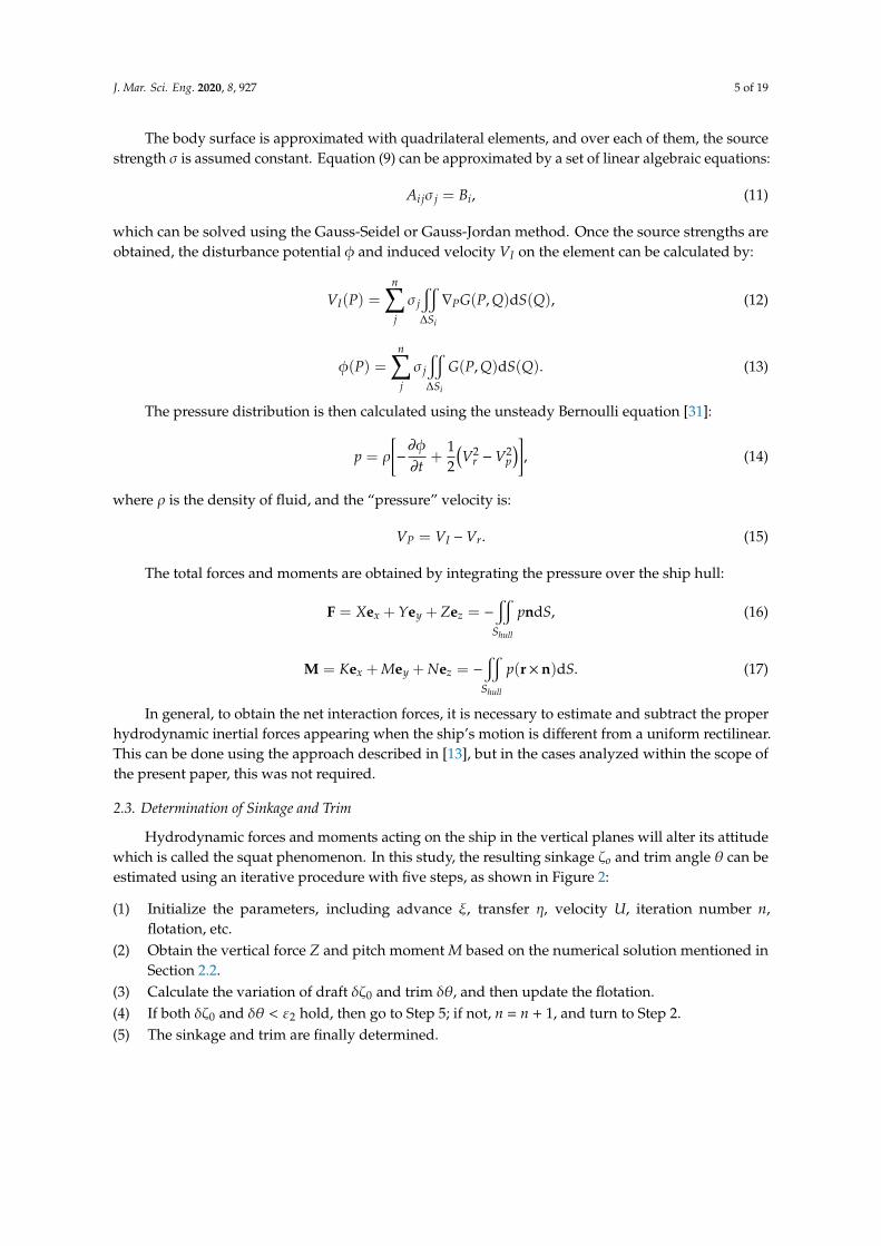
The pressure distribution is then calculated using the unsteady Bernoulli equation [31]:

p = ρ

[−∂φ

∂t+

12

(V2

r −V2p

)], (14)

where ρ is the density of fluid, and the “pressure” velocity is:

VP = VI −Vr. (15)

The total forces and moments are obtained by integrating the pressure over the ship hull:

F = Xex + Yey + Zez = −x

Shull

pndS, (16)

M = Kex + Mey + Nez = −x

Shull

p(r× n)dS. (17)

In general, to obtain the net interaction forces, it is necessary to estimate and subtract the properhydrodynamic inertial forces appearing when the ship’s motion is different from a uniform rectilinear.This can be done using the approach described in [13], but in the cases analyzed within the scope ofthe present paper, this was not required.

2.3. Determination of Sinkage and Trim

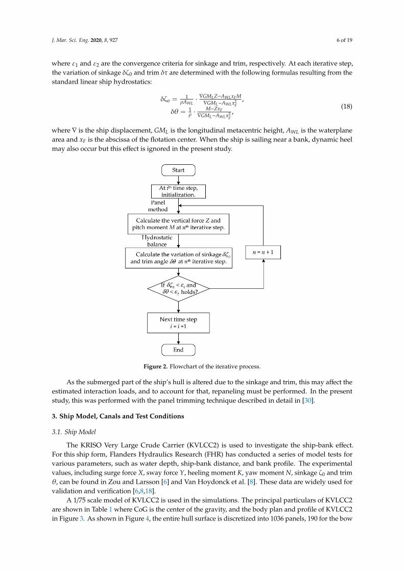
Hydrodynamic forces and moments acting on the ship in the vertical planes will alter its attitudewhich is called the squat phenomenon. In this study, the resulting sinkage ζo and trim angle θ can beestimated using an iterative procedure with five steps, as shown in Figure 2:

(1) Initialize the parameters, including advance ξ, transfer η, velocity U, iteration number n,flotation, etc.

(2) Obtain the vertical force Z and pitch moment M based on the numerical solution mentioned inSection 2.2.

(3) Calculate the variation of draft δζ0 and trim δθ, and then update the flotation.(4) If both δζ0 and δθ < ε2 hold, then go to Step 5; if not, n = n + 1, and turn to Step 2.(5) The sinkage and trim are finally determined.

J. Mar. Sci. Eng. 2020, 8, 927 6 of 19

where ε1 and ε2 are the convergence criteria for sinkage and trim, respectively. At each iterative step,the variation of sinkage δζ0 and trim δτ are determined with the following formulas resulting from thestandard linear ship hydrostatics:

δζo =1

ρAWL·∇GMLZ−AWLxFM∇GML−AWLx2

F,

δθ = 1ρ ·

M−ZxF∇GML−AWLx2

F,

(18)

where ∇ is the ship displacement, GML is the longitudinal metacentric height, AWL is the waterplanearea and xF is the abscissa of the flotation center. When the ship is sailing near a bank, dynamic heelmay also occur but this effect is ignored in the present study.

J. Mar. Sci. Eng. 2020, 8, x FOR PEER REVIEW 6 of 20

2

2

1,

1,

L WL Fo

WL L WL F

F

L WL F

GM Z A x M

A GM A x

M Zx

GM A x

(18)

where is the ship displacement, LGM is the longitudinal metacentric height, WL

A is the

waterplane area and Fx is the abscissa of the flotation center. When the ship is sailing near a bank,

dynamic heel may also occur but this effect is ignored in the present study.

As the submerged part of the ship’s hull is altered due to the sinkage and trim, this may affect

the estimated interaction loads, and to account for that, repaneling must be performed. In the

present study, this was performed with the panel trimming technique described in detail in [30].

Figure 2. Flowchart of the iterative process.

3. Ship Model, Canals and Test Conditions

3.1. Ship Model

The KRISO Very Large Crude Carrier (KVLCC2) is used to investigate the ship-bank effect. For

this ship form, Flanders Hydraulics Research (FHR) has conducted a series of model tests for various

parameters, such as water depth, ship-bank distance, and bank profile. The experimental values,

including surge force X , sway force Y , heeling moment K , yaw moment N , sinkage 0 and

trim , can be found in Zou and Larsson [6] and Van Hoydonck et al. [8]. These data are widely used

for validation and verification [6,8,18].

A 1/75 scale model of KVLCC2 is used in the simulations. The principal particulars of KVLCC2

are shown in Table 1 where CoG is the center of the gravity, and the body plan and profile of

KVLCC2 in Figure 3. As shown in Figure 4, the entire hull surface is discretized into 1036 panels, 190

for the bow ( 1.706mx ), 704 for the parallel body ( 1.706m 1.706mx ), and 142 for the stern

Figure 2. Flowchart of the iterative process.

As the submerged part of the ship’s hull is altered due to the sinkage and trim, this may affect theestimated interaction loads, and to account for that, repaneling must be performed. In the presentstudy, this was performed with the panel trimming technique described in detail in [30].

3. Ship Model, Canals and Test Conditions

3.1. Ship Model

The KRISO Very Large Crude Carrier (KVLCC2) is used to investigate the ship-bank effect.For this ship form, Flanders Hydraulics Research (FHR) has conducted a series of model tests forvarious parameters, such as water depth, ship-bank distance, and bank profile. The experimentalvalues, including surge force X, sway force Y, heeling moment K, yaw moment N, sinkage ζ0 and trimθ, can be found in Zou and Larsson [6] and Van Hoydonck et al. [8]. These data are widely used forvalidation and verification [6,8,18].

A 1/75 scale model of KVLCC2 is used in the simulations. The principal particulars of KVLCC2are shown in Table 1 where CoG is the center of the gravity, and the body plan and profile of KVLCC2in Figure 3. As shown in Figure 4, the entire hull surface is discretized into 1036 panels, 190 for the bow

J. Mar. Sci. Eng. 2020, 8, 927 7 of 19

(x > 1.706 m), 704 for the parallel body (−1.706 m ≤ x ≤ 1.706 m), and 142 for the stern (x < −1.706 m).The panels used for simulation are generated from the mesh for the entire hull surface and vary withthe predicted sinkage and trim. The discretization of the portion below the instantaneous waterlineat the initial instant (0.2776 m draft, 0◦ trim) is shown in Figure 5, where 874 panels are used toapproximate the wetted surface, which has been proven sufficient for ship hydrodynamic interactionsimulations [13].

Table 1. Principle particulars of the KRISO Very Large Crude Carrier (KVLCC2) in full-scale andmodel scale.

Parameters Full Scale Model Scale

Length (LPP) (m) 320.0 4.2667Breath (B) (m) 58.0 0.7733

Draft at midship (T) (m) 20.8 0.2776Longitudinal CoG (xG) (m) 10.87 0.1449

Vertical CoG (zG) (m) 20.8 0.2776Longitudinal CoF (xw) (m) −2.67 −0.0356Waterplane area (Aw) (m2) 16,706.25 2.9700

Displacement (∇) (m3) 312,622 0.7410Longitudinal metacentric height (GML) (m) 398.55 5.3140

Block coefficient (CB) 0.8098 0.8098

J. Mar. Sci. Eng. 2020, 8, x FOR PEER REVIEW 7 of 20

( 1.706mx ). The panels used for simulation are generated from the mesh for the entire hull

surface and vary with the predicted sinkage and trim. The discretization of the portion below the

instantaneous waterline at the initial instant (0.2776 m draft, 0 trim) is shown in Figure 5, where

874 panels are used to approximate the wetted surface, which has been proven sufficient for ship

hydrodynamic interaction simulations [13].

Table 1. Principle particulars of the KRISO Very Large Crude Carrier (KVLCC2) in full-scale and

model scale.

Parameters Full Scale Model Scale

Length ( PPL ) (m) 320.0 4.2667

Breath ( B ) (m) 58.0 0.7733

Draft at midship ( T ) (m) 20.8 0.2776

Longitudinal CoG ( Gx ) (m) 10.87 0.1449

Vertical CoG ( Gz ) (m) 20.8 0.2776

Longitudinal CoF ( wx ) (m) −2.67 −0.0356

Waterplane area ( wA ) (m2) 16,706.25 2.9700

Displacement ( ) (m3) 312622 0.7410

Longitudinal metacentric height ( LGM ) (m) 398.55 5.3140

Block coefficient ( BC ) 0.8098 0.8098

Figure 3. Body plan and profile of the KRISO Very Large Crude Carrier (KVLCC2).

Figure 4. Discretization of the entire hull surface.

Figure 3. Body plan and profile of the KRISO Very Large Crude Carrier (KVLCC2).

J. Mar. Sci. Eng. 2020, 8, x FOR PEER REVIEW 7 of 20

( 1.706mx ). The panels used for simulation are generated from the mesh for the entire hull

surface and vary with the predicted sinkage and trim. The discretization of the portion below the

instantaneous waterline at the initial instant (0.2776 m draft, 0 trim) is shown in Figure 5, where

874 panels are used to approximate the wetted surface, which has been proven sufficient for ship

hydrodynamic interaction simulations [13].

Table 1. Principle particulars of the KRISO Very Large Crude Carrier (KVLCC2) in full-scale and

model scale.

Parameters Full Scale Model Scale

Length ( PPL ) (m) 320.0 4.2667

Breath ( B ) (m) 58.0 0.7733

Draft at midship ( T ) (m) 20.8 0.2776

Longitudinal CoG ( Gx ) (m) 10.87 0.1449

Vertical CoG ( Gz ) (m) 20.8 0.2776

Longitudinal CoF ( wx ) (m) −2.67 −0.0356

Waterplane area ( wA ) (m2) 16,706.25 2.9700

Displacement ( ) (m3) 312622 0.7410

Longitudinal metacentric height ( LGM ) (m) 398.55 5.3140

Block coefficient ( BC ) 0.8098 0.8098

Figure 3. Body plan and profile of the KRISO Very Large Crude Carrier (KVLCC2).

Figure 4. Discretization of the entire hull surface. Figure 4. Discretization of the entire hull surface.

J. Mar. Sci. Eng. 2020, 8, 927 8 of 19J. Mar. Sci. Eng. 2020, 8, x FOR PEER REVIEW 8 of 20

Figure 5. Discretization of the wetted surface at outset.

3.2. The Canals

Two different canal profiles were investigated: Canal A and Canal B. The former has a vertical

wall on the right-hand side and a 1:4 slope bank is on the other. The latter has two sloped banks, one

of which has a slope of 1:1, and the other a slope of 1:3, as shown in Figure 6. The lateral distance

between the center-plane of the ship and the bottom of the bank is denoted as ys.

Figure 6. Profiles of the two canals.

In the application of the paneled moving patch method, sources are distributed; in addition to

the wetted hull surface, also over some finite domain (patch) of the bottom beneath the moving hull,

and this patch moves with the ship so as to take into account the bottom and bank effect in the

simulation. Both the panel size and the dimensions of the patch directly affect the computational

efficiency. Larger patches and finer grids will produce better accuracy, while the computational cost

also increases. For this reason, a convergence analysis is performed to determine the size of patch

and panel for the canal. For the patch size, a set of calculations with various patch length is carried

out where the length of the patch on the canal bed/bank ranges from 6 m to 22 m, and

square-shaped panels with a side length of 0.2 m are used. The KVLCC2 model was moving along

the bank in Canal A at a constant speed of 0.356 m/s, with the depth-to-draft ratio / 1.35h T , and

the ship-bank distance 0.5175ms

y . The numerical results with varying patch length are obtained

and plotted in Figure 7. As can be seen from all the numerical results for the forces, sinkage and trim

converge as the patch length increases.

Figure 5. Discretization of the wetted surface at outset.

3.2. The Canals

Two different canal profiles were investigated: Canal A and Canal B. The former has a verticalwall on the right-hand side and a 1:4 slope bank is on the other. The latter has two sloped banks, one ofwhich has a slope of 1:1, and the other a slope of 1:3, as shown in Figure 6. The lateral distance betweenthe center-plane of the ship and the bottom of the bank is denoted as ys.

J. Mar. Sci. Eng. 2020, 8, x FOR PEER REVIEW 8 of 20

Figure 5. Discretization of the wetted surface at outset.

3.2. The Canals

Two different canal profiles were investigated: Canal A and Canal B. The former has a vertical

wall on the right-hand side and a 1:4 slope bank is on the other. The latter has two sloped banks, one

of which has a slope of 1:1, and the other a slope of 1:3, as shown in Figure 6. The lateral distance

between the center-plane of the ship and the bottom of the bank is denoted as ys.

Figure 6. Profiles of the two canals.

In the application of the paneled moving patch method, sources are distributed; in addition to

the wetted hull surface, also over some finite domain (patch) of the bottom beneath the moving hull,

and this patch moves with the ship so as to take into account the bottom and bank effect in the

simulation. Both the panel size and the dimensions of the patch directly affect the computational

efficiency. Larger patches and finer grids will produce better accuracy, while the computational cost

also increases. For this reason, a convergence analysis is performed to determine the size of patch

and panel for the canal. For the patch size, a set of calculations with various patch length is carried

out where the length of the patch on the canal bed/bank ranges from 6 m to 22 m, and

square-shaped panels with a side length of 0.2 m are used. The KVLCC2 model was moving along

the bank in Canal A at a constant speed of 0.356 m/s, with the depth-to-draft ratio / 1.35h T , and

the ship-bank distance 0.5175ms

y . The numerical results with varying patch length are obtained

and plotted in Figure 7. As can be seen from all the numerical results for the forces, sinkage and trim

converge as the patch length increases.

Figure 6. Profiles of the two canals.

In the application of the paneled moving patch method, sources are distributed; in additionto the wetted hull surface, also over some finite domain (patch) of the bottom beneath the movinghull, and this patch moves with the ship so as to take into account the bottom and bank effect in thesimulation. Both the panel size and the dimensions of the patch directly affect the computationalefficiency. Larger patches and finer grids will produce better accuracy, while the computational costalso increases. For this reason, a convergence analysis is performed to determine the size of patch andpanel for the canal. For the patch size, a set of calculations with various patch length is carried outwhere the length of the patch on the canal bed/bank ranges from 6 m to 22 m, and square-shapedpanels with a side length of 0.2 m are used. The KVLCC2 model was moving along the bank in CanalA at a constant speed of 0.356 m/s, with the depth-to-draft ratio h/T = 1.35, and the ship-bank distanceys = 0.5175 m. The numerical results with varying patch length are obtained and plotted in Figure 7.As can be seen from all the numerical results for the forces, sinkage and trim converge as the patchlength increases.

J. Mar. Sci. Eng. 2020, 8, 927 9 of 19

J. Mar. Sci. Eng. 2020, 8, x FOR PEER REVIEW 9 of 20

Figure 7. Numerical results obtained with various patch lengths for the case of Canal A.

It can be observed from Figure 7 that a larger patch length can improve the accuracy while the

computational cost is also higher. Therefore, it is unwise to use extra-large patch sizes when the

computational efficiency is also a concern. According to the convergence analysis, the patch length

of 18 m is chosen for the simulations in this study, i.e., 4.22 times the model length of KVLCC2.

A similar convergence analysis is carried out to determine the panel size for the canal with the

panel size ranging from 0.15 m to 1.0 m, and the patch length takes 18 m according to the

convergence pattern in Figure 7. The test case used in the convergence analysis of the patch length

is used, and the numerical results calculated with different panel sizes are shown in Figure 8. It is

found that the results are well behaved when the panel size is smaller than 0.25 m. Since there are

cases with shallower water depths and smaller ship-bank distances in the study, the panel size for

the canal takes 0.2 m so as to obtain reliable results. The discretization of Canal A is shown in Figure

9, where the maximum panel size is 0.2 m.

Figure 8. Numerical results obtained with various panel sizes for the case of Canal A.

Figure 7. Numerical results obtained with various patch lengths for the case of Canal A.

It can be observed from Figure 7 that a larger patch length can improve the accuracy while thecomputational cost is also higher. Therefore, it is unwise to use extra-large patch sizes when thecomputational efficiency is also a concern. According to the convergence analysis, the patch length of18 m is chosen for the simulations in this study, i.e., 4.22 times the model length of KVLCC2.

A similar convergence analysis is carried out to determine the panel size for the canal with thepanel size ranging from 0.15 m to 1.0 m, and the patch length takes 18 m according to the convergencepattern in Figure 7. The test case used in the convergence analysis of the patch length is used, and thenumerical results calculated with different panel sizes are shown in Figure 8. It is found that the resultsare well behaved when the panel size is smaller than 0.25 m. Since there are cases with shallower waterdepths and smaller ship-bank distances in the study, the panel size for the canal takes 0.2 m so as toobtain reliable results. The discretization of Canal A is shown in Figure 9, where the maximum panelsize is 0.2 m.

J. Mar. Sci. Eng. 2020, 8, x FOR PEER REVIEW 9 of 20

Figure 7. Numerical results obtained with various patch lengths for the case of Canal A.

It can be observed from Figure 7 that a larger patch length can improve the accuracy while the

computational cost is also higher. Therefore, it is unwise to use extra-large patch sizes when the

computational efficiency is also a concern. According to the convergence analysis, the patch length

of 18 m is chosen for the simulations in this study, i.e., 4.22 times the model length of KVLCC2.

A similar convergence analysis is carried out to determine the panel size for the canal with the

panel size ranging from 0.15 m to 1.0 m, and the patch length takes 18 m according to the

convergence pattern in Figure 7. The test case used in the convergence analysis of the patch length

is used, and the numerical results calculated with different panel sizes are shown in Figure 8. It is

found that the results are well behaved when the panel size is smaller than 0.25 m. Since there are

cases with shallower water depths and smaller ship-bank distances in the study, the panel size for

the canal takes 0.2 m so as to obtain reliable results. The discretization of Canal A is shown in Figure

9, where the maximum panel size is 0.2 m.

Figure 8. Numerical results obtained with various panel sizes for the case of Canal A.

Figure 8. Numerical results obtained with various panel sizes for the case of Canal A.

J. Mar. Sci. Eng. 2020, 8, 927 10 of 19J. Mar. Sci. Eng. 2020, 8, x FOR PEER REVIEW 10 of 20

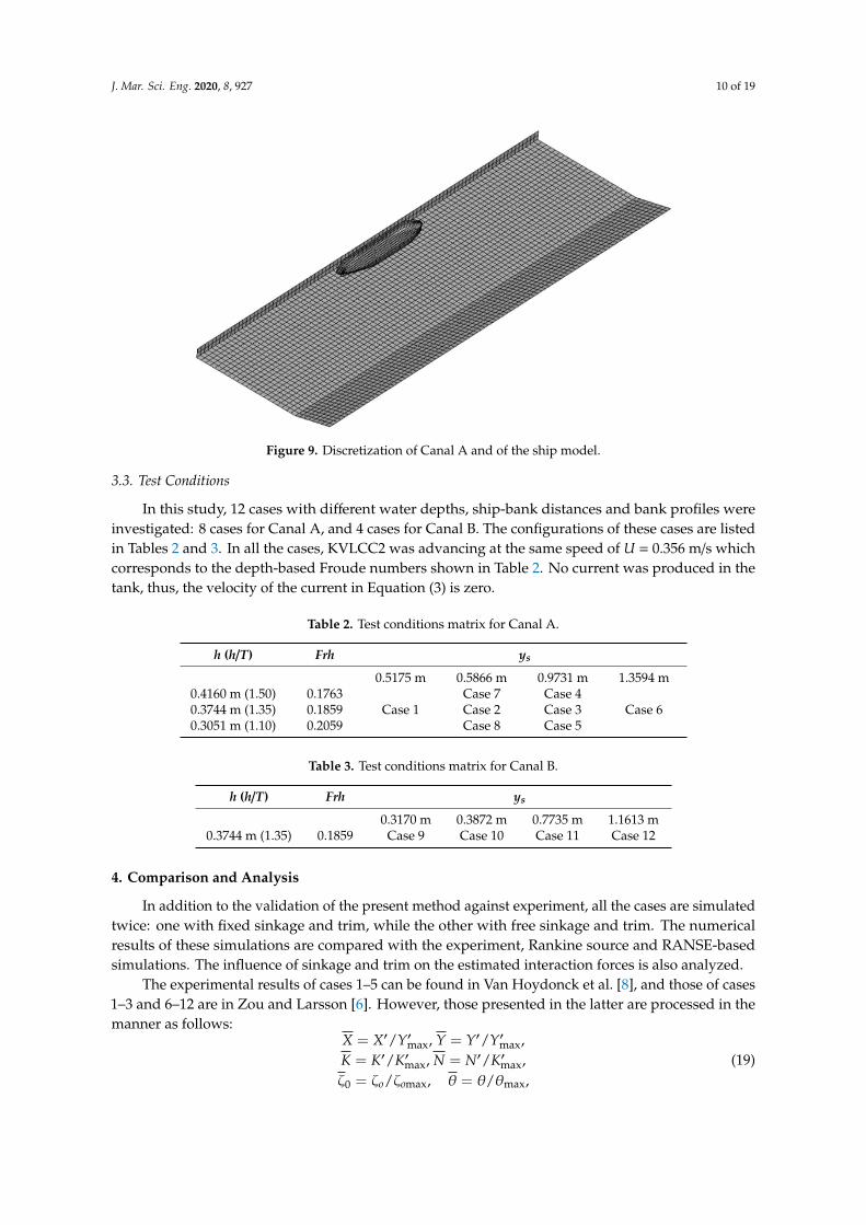
Figure 9. Discretization of Canal A and of the ship model.

3.3. Test Conditions

In this study, 12 cases with different water depths, ship-bank distances and bank profiles were

investigated: 8 cases for Canal A, and 4 cases for Canal B. The configurations of these cases are listed

in Tables 2 and 3. In all the cases, KVLCC2 was advancing at the same speed of U = 0.356 m/s which

corresponds to the depth-based Froude numbers shown in Table 2. No current was produced in the

tank, thus, the velocity of the current in Equation (3) is zero.

Table 2. Test conditions matrix for Canal A.

h (h/T) Frh ys

0.5175 m 0.5866 m 0.9731 m 1.3594 m

0.4160 m (1.50) 0.1763 Case 7 Case 4

0.3744 m (1.35) 0.1859 Case 1 Case 2 Case 3 Case 6

0.3051 m (1.10) 0.2059 Case 8 Case 5

Table 3. Test conditions matrix for Canal B.

h (h/T) Frh ys

0.3170 m 0.3872 m 0.7735 m 1.1613 m

0.3744 m (1.35) 0.1859 Case 9 Case 10 Case 11 Case 12

4. Comparison and Analysis

In addition to the validation of the present method against experiment, all the cases are

simulated twice: one with fixed sinkage and trim, while the other with free sinkage and trim. The

numerical results of these simulations are compared with the experiment, Rankine source and

RANSE-based simulations. The influence of sinkage and trim on the estimated interaction forces is

also analyzed.

The experimental results of cases 1–5 can be found in Van Hoydonck et al. [8], and those of

cases 1–3 and 6–12 are in Zou and Larsson [6]. However, those presented in the latter are processed

in the manner as follows:

Figure 9. Discretization of Canal A and of the ship model.

3.3. Test Conditions

In this study, 12 cases with different water depths, ship-bank distances and bank profiles wereinvestigated: 8 cases for Canal A, and 4 cases for Canal B. The configurations of these cases are listedin Tables 2 and 3. In all the cases, KVLCC2 was advancing at the same speed of U = 0.356 m/s whichcorresponds to the depth-based Froude numbers shown in Table 2. No current was produced in thetank, thus, the velocity of the current in Equation (3) is zero.

Table 2. Test conditions matrix for Canal A.

h (h/T) Frh ys

0.5175 m 0.5866 m 0.9731 m 1.3594 m0.4160 m (1.50) 0.1763 Case 7 Case 40.3744 m (1.35) 0.1859 Case 1 Case 2 Case 3 Case 60.3051 m (1.10) 0.2059 Case 8 Case 5

Table 3. Test conditions matrix for Canal B.

h (h/T) Frh ys

0.3170 m 0.3872 m 0.7735 m 1.1613 m0.3744 m (1.35) 0.1859 Case 9 Case 10 Case 11 Case 12

4. Comparison and Analysis

In addition to the validation of the present method against experiment, all the cases are simulatedtwice: one with fixed sinkage and trim, while the other with free sinkage and trim. The numericalresults of these simulations are compared with the experiment, Rankine source and RANSE-basedsimulations. The influence of sinkage and trim on the estimated interaction forces is also analyzed.

The experimental results of cases 1–5 can be found in Van Hoydonck et al. [8], and those of cases1–3 and 6–12 are in Zou and Larsson [6]. However, those presented in the latter are processed in themanner as follows:

X = X′/Y′max, Y = Y′/Y′max,K = K′/K′max, N = N′/K′max,ζ0 = ζo/ζomax, θ = θ/θmax,

(19)

J. Mar. Sci. Eng. 2020, 8, 927 11 of 19

where X′, Y′, K′, N′, are the nondimensionalized values for surge force, sway force, heeling momentand yaw moment:

X′ = X12ρU2LppT

, Y′ = Y12ρU2LppT

,

K′ = K12ρU2LppT2 , N′ = N

12ρU2L2

PPT.

(20)

The subscript ‘max’ in Equation (19) denotes the maximum measures appeared in all the casesinvestigated in the study, which, however, are not explicitly given in the publication [6]; and the bar ontop of a symbols stands for relative values.

Since the same cases, i.e., cases 1–3, are presented in both Van Hoydonck et al. [8] and Zou andLarsson [6], the maximum measures undisclosed in Zou and Larsson [6] can be calculated from theabsolute experimental values provided in Van Hoydonck et al. [8], and the absolute values of the cases6–12 can be adopted. For example, for the sway force, the non-dimensional results Y′i (i = 1, 2, 3) forthe cases 1–3 can be calculated from the absolute values Yi (i = 1, 2, 3) given in Van Hoydonck et al. [8],and then Y′max in Equation (19) can be calculated Y′max = Y′i /Yi as Yi (i = 1, 2, 3) is given inZou and Larsson [6]. This Y′max also applied to the processing of the results of cases 6–12, thus,Y′i = Yi ×Y′max (i = 6, . . . , 12), and finally, the absolute values Yi (i = 6, . . . , 12) of the cases 6–12 canbe obtained using Equation (20).

Besides the test data, comparisons with the RANSE-based method [6,8] and the Rankine sourcemethod [18] have also been carried out whenever possible.

4.1. Sinkage and Trim in Canal A

The numerical results obtained with the present method for the sinkage and trim in Canal Aare plotted in Figures 10–12, together with the experimental ones as those obtained with the RANSEcode: EFD in the legends corresponds to the experimental results, CFD—to the RANSE simulations,and Rankine—to the results obtained by the free-surface Rankine source method.

As shown in Figure 10, the sinkage and trim increase with reduction of the ship-bank distance,and a significant bank influence on the squat is observed. The estimated sinkage and trim with variousratios of h/T at two different ship-bank distances are plotted in Figures 11 and 12. It can also be seenthat the sinkage and trim increase as the water depth reduces.

J. Mar. Sci. Eng. 2020, 8, x FOR PEER REVIEW 12 of 20

4.2. Hydrodynamic Forces and Moments in Canal A

The estimated interaction forces and moments of KVLCC2 moving in parallel to the vertical

wall are plotted in Figure 13 as a function of ship-bank distance ys, where the results of model test,

viscous flow simulation, and Rankine source method are also given for the purpose of comparison.

The numerical results with/without accounting for sinkage and trim are both presented in this

section as to analyze their contribution to the hydrodynamic interaction forces.

(a) (b)

Figure 10. Sinkage and trim at the different lateral distance ys at h/T = 1.35. (a) Sinkage (b) Trim.

(a) (b)

Figure 11. Sinkage and trim at the different ratios of h/T at ys = 0.5866 m. (a) Sinkage (b) Trim.

Figure 10. Sinkage and trim at the different lateral distance ys at h/T = 1.35. (a) Sinkage (b) Trim.

J. Mar. Sci. Eng. 2020, 8, 927 12 of 19

J. Mar. Sci. Eng. 2020, 8, x FOR PEER REVIEW 12 of 20

4.2. Hydrodynamic Forces and Moments in Canal A

The estimated interaction forces and moments of KVLCC2 moving in parallel to the vertical

wall are plotted in Figure 13 as a function of ship-bank distance ys, where the results of model test,

viscous flow simulation, and Rankine source method are also given for the purpose of comparison.

The numerical results with/without accounting for sinkage and trim are both presented in this

section as to analyze their contribution to the hydrodynamic interaction forces.

(a) (b)

Figure 10. Sinkage and trim at the different lateral distance ys at h/T = 1.35. (a) Sinkage (b) Trim.

(a) (b)

Figure 11. Sinkage and trim at the different ratios of h/T at ys = 0.5866 m. (a) Sinkage (b) Trim. Figure 11. Sinkage and trim at the different ratios of h/T at ys = 0.5866 m. (a) Sinkage (b) Trim.J. Mar. Sci. Eng. 2020, 8, x FOR PEER REVIEW 13 of 20

(a) (b)

Figure 12. Sinkage and trim at the different ratios of h/T at ys = 0.9731 m. (a) Sinkage (b) Trim.

(a) (b)

(c)

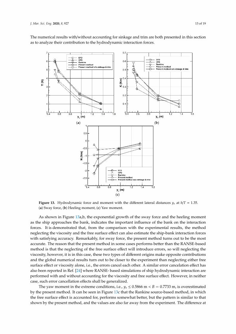
Figure 13. Hydrodynamic force and moment with the different lateral distances ys at h/T = 1.35. (a)

Sway force, (b) Heeling moment, (c) Yaw moment.

Figure 12. Sinkage and trim at the different ratios of h/T at ys = 0.9731 m. (a) Sinkage (b) Trim.

Regarding the sinkage, the tendencies are well captured with the present numerical method.It can be also observed from the figures that, the present method, in general, somewhat underestimatesthe sinkage, and the discrepancy becomes larger as the ship gets closer to the bank and the bottom,especially, for the extreme condition of h/T = 1.1. The RANSE-based method is more accurate,which suggests that the viscous effect is non-negligible in this case, as shown in Figure 11a. On theother hand, the free surface effect seems to be insignificant as long as it was not considered in theviscous flow simulations [18].

The stern down trim due to the bank effect is also captured by the present method with fairaccuracy, even if the viscosity effect and free surface effect are both neglected. As shown in Figure 11b,the error in the estimate for the trim is still acceptable for the most extreme condition, i.e., h/T = 1.1 andys = 0.5866 m. Comparison of the present method with the RANSE-based simulation of the case ofh/T = 1.1 shows that RANSE-based simulation accounting for viscosity is not more accurate becausethe estimates for the trim by both methods are almost the same.

4.2. Hydrodynamic Forces and Moments in Canal A

The estimated interaction forces and moments of KVLCC2 moving in parallel to the verticalwall are plotted in Figure 13 as a function of ship-bank distance ys, where the results of model test,viscous flow simulation, and Rankine source method are also given for the purpose of comparison.

J. Mar. Sci. Eng. 2020, 8, 927 13 of 19

The numerical results with/without accounting for sinkage and trim are both presented in this sectionas to analyze their contribution to the hydrodynamic interaction forces.

J. Mar. Sci. Eng. 2020, 8, x FOR PEER REVIEW 13 of 20

(a) (b)

Figure 12. Sinkage and trim at the different ratios of h/T at ys = 0.9731 m. (a) Sinkage (b) Trim.

(a) (b)

(c)

Figure 13. Hydrodynamic force and moment with the different lateral distances ys at h/T = 1.35. (a)

Sway force, (b) Heeling moment, (c) Yaw moment. Figure 13. Hydrodynamic force and moment with the different lateral distances ys at h/T = 1.35.(a) Sway force, (b) Heeling moment, (c) Yaw moment.

As shown in Figure 13a,b, the exponential growth of the sway force and the heeling momentas the ship approaches the bank, indicates the important influence of the bank on the interactionforces. It is demonstrated that, from the comparison with the experimental results, the methodneglecting the viscosity and the free surface effect can also estimate the ship-bank interaction forceswith satisfying accuracy. Remarkably, for sway force, the present method turns out to be the mostaccurate. The reason that the present method in some cases performs better than the RANSE-basedmethod is that the neglecting of the free surface effect will introduce errors, so will neglecting theviscosity, however, it is in this case, these two types of different origins make opposite contributionsand the global numerical results turn out to be closer to the experiment than neglecting either freesurface effect or viscosity alone, i.e., the errors cancel each other. A similar error cancelation effect hasalso been reported in Ref. [24] where RANSE- based simulations of ship hydrodynamic interaction areperformed with and without accounting for the viscosity and free surface effect. However, in neithercase, such error cancellation effects shall be generalized.

The yaw moment in the extreme conditions, i.e., ys ≤ 0.5866 m < B = 0.7733 m, is overestimatedby the present method. It can be seen in Figure 13c that the Rankine source-based method, in whichthe free surface effect is accounted for, performs somewhat better, but the pattern is similar to thatshown by the present method, and the values are also far away from the experiment. The difference at

J. Mar. Sci. Eng. 2020, 8, 927 14 of 19

ys ≤ 0.5866 m may be caused by the drop of the free surface drop at the side of bank, and the influenceof free surface also plays a significant role on yaw moment at a relatively small ship-bank distanceeven in the intermediate water depth. The RANSE-based code also failed to produce a reasonableestimate in this case. For larger ship-bank distances ys, the pattern of the yaw moment obtained by thepresent method is similar to the experiment, however, there is still a difference, as shown in Figure 13c.Interestingly, the present method shows a very good agreement with both RANSE-based simulationand the Rankine source-based method. It seems that considering the free surface effect or the viscosityalone in the numerical methods does not help much with producing more accurate results in this case.

The hydrodynamic interaction forces and moments at ys = 0.5866 m and ys = 0.9731 m arepresented in Figures 14 and 15 as function of the relative water depth. As shown in Figures 14a and 15a,the present method, in general, overestimates the sway force for the case of the extreme shallowwater (h/T = 1.1). Actually, the effect of the free surface is significant in very confined waters [8],the level difference between both sides of the hull is relatively large, and the double-body model isnot suitable in these cases—in which cases, the Rankine source method performs better. Accountingfor the sinkage and trim helps with the accuracy of the calculation for both ship-bank distances,while the improvement is small which could be expected at small changes of attitude. A comparison ofFigures 14a and 15a shows that the present method is less accurate as the ship-bank distance decreasesfrom ys = 0.9731 m to ys = 0.5866 m, but still the relative error is smaller than 15% (except for theextreme shallow water case). This suggests that the present method is fairly accurate in estimating thesway force for moderate shallowness.J. Mar. Sci. Eng. 2020, 8, x FOR PEER REVIEW 15 of 20

(a) (b)

(c)

Figure 14. Hydrodynamic force and moment at the different ratios of h/T at ys = 0.5866 m. (a) Sway

force, (b) Heeling moment, (c) Yaw moment.

(a) (b)

Figure 14. Hydrodynamic force and moment at the different ratios of h/T at ys = 0.5866 m. (a) Swayforce, (b) Heeling moment, (c) Yaw moment.

J. Mar. Sci. Eng. 2020, 8, 927 15 of 19

J. Mar. Sci. Eng. 2020, 8, x FOR PEER REVIEW 15 of 20

(a) (b)

(c)

Figure 14. Hydrodynamic force and moment at the different ratios of h/T at ys = 0.5866 m. (a) Sway

force, (b) Heeling moment, (c) Yaw moment.

(a) (b) J. Mar. Sci. Eng. 2020, 8, x FOR PEER REVIEW 16 of 20

(c)

Figure 15. Hydrodynamic force and moment at the different ratios of h/T at ys = 0.9731 m. (a) Sway

force, (b) Heeling moment, (c) Yaw moment.

For the heeling moment, the numerical results obtained by the present method have a pattern

similar to the experiment. For the case of ys = 0.5866 m, the heeling moment is slightly

underestimated by the present method at h/T = 1.1. For larger ratios of h/T, all the numerical

approaches produce almost the same results that are overestimated to some extent, with a relatively

larger error at h/T = 1.35 and a smaller error at h/T = 1.50, as shown in Figure 14(b). At ys = 0.9731 m,

the pattern is correctly captured by the present method, with a slight underestimation for the case

h/T = 1.1 and some overestimation for other water depths. In comparison, the RANSE-based method

fails to estimate the force at h/T = 1.1, but looks very accurate for other water depths. Based on the

comparisons for the heeling moment as shown in the Figures 13b–15b, it can be stated that the

present method is able to estimate the heeling moment with a fair accuracy.

For ys = 0.5866 m and h/T = 1.1, the yaw moment is significantly underestimated by the present

method. In this case, only the RANSE-based method was able to give reasonable estimates. For

other water depths at the same ship-bank distance, however, the present method performed even

better than the RANSE-based method in terms of accuracy. A possible reason for the better

accuracy of the present method than the RANSE-based method in neglecting the free surface effect

is that there might be a cancellation effect between the errors resulted from neglecting the free

surface effect and those from neglecting the viscosity. For ys = 0.9731 m, the present method

produces almost the same results as the Rankine source-based method, and both of them failed to

estimate the yaw moment for the extreme shallow water case of h/T = 1.1. For other water depths,

the present method and the Rankine source-based method agree well with the experiment. Thus, as

can be seen from the comparisons, the present method is also able to estimate the yaw moment

except for the extreme shallow water case, which, however, should be avoided in navigation [32].

4.3. Sinkage and Trim in Canal B

In this section, a set of simulations of KVLCC2 moving along a sloped bank is carried out, and

the results for the sinkage and trim with various lateral distances are plotted in Figure 16. It can be

seen that the smaller is the ship-bank distance, the larger is the sinkage and trim.

For the sinkage, this trend is well captured by both the RANSE-based method and the present

method. The former is very accurate, while the latter exhibits the error of 19% for the smallest bank

distance, which reduces to 10% as the distance increases.

The superiority of the RANSE-based method is very limited in the calculation of the trim, as

shown in Figure 16b, and, in fact, for the small ship-bank distances, the present methods even

produce more accurate results. For all investigated ship-bank distances, the relative error of the

Figure 15. Hydrodynamic force and moment at the different ratios of h/T at ys = 0.9731 m. (a) Swayforce, (b) Heeling moment, (c) Yaw moment.

For the heeling moment, the numerical results obtained by the present method have a patternsimilar to the experiment. For the case of ys = 0.5866 m, the heeling moment is slightly underestimatedby the present method at h/T = 1.1. For larger ratios of h/T, all the numerical approaches produce almostthe same results that are overestimated to some extent, with a relatively larger error at h/T = 1.35 and asmaller error at h/T = 1.50, as shown in Figure 14b. At ys = 0.9731 m, the pattern is correctly capturedby the present method, with a slight underestimation for the case h/T = 1.1 and some overestimationfor other water depths. In comparison, the RANSE-based method fails to estimate the force at h/T = 1.1,but looks very accurate for other water depths. Based on the comparisons for the heeling moment asshown in the Figures 13b, 14b and 15b, it can be stated that the present method is able to estimate theheeling moment with a fair accuracy.

For ys = 0.5866 m and h/T = 1.1, the yaw moment is significantly underestimated by the presentmethod. In this case, only the RANSE-based method was able to give reasonable estimates. For otherwater depths at the same ship-bank distance, however, the present method performed even betterthan the RANSE-based method in terms of accuracy. A possible reason for the better accuracy of thepresent method than the RANSE-based method in neglecting the free surface effect is that there mightbe a cancellation effect between the errors resulted from neglecting the free surface effect and thosefrom neglecting the viscosity. For ys = 0.9731 m, the present method produces almost the same resultsas the Rankine source-based method, and both of them failed to estimate the yaw moment for the

J. Mar. Sci. Eng. 2020, 8, 927 16 of 19

extreme shallow water case of h/T = 1.1. For other water depths, the present method and the Rankinesource-based method agree well with the experiment. Thus, as can be seen from the comparisons,the present method is also able to estimate the yaw moment except for the extreme shallow water case,which, however, should be avoided in navigation [32].

4.3. Sinkage and Trim in Canal B

In this section, a set of simulations of KVLCC2 moving along a sloped bank is carried out, and theresults for the sinkage and trim with various lateral distances are plotted in Figure 16. It can be seenthat the smaller is the ship-bank distance, the larger is the sinkage and trim.

J. Mar. Sci. Eng. 2020, 8, x FOR PEER REVIEW 17 of 20

present method remains within the range from 12% to 18%. The discrepancies likely result from

neglecting the free surface viscosity effects.

In general, the present method is able to produce results for the sinkage and trim with

acceptable accuracy.

(a) (b)

Figure 16. Sinkage and trim with the different lateral positions at h/T = 1.35. (a) Sinkage, (b) Trim.

4.4. Hydrodynamic Forces and Moments in Canal B

The results for the interaction forces in Canal B obtained by the present method with and

without accounting for sinkage and trim are plotted in Figure 17. Similarly to the case of the vertical

bank wall, the forces increase as the ship-bank distance decreases. The sinkage is slightly

underestimated but the accuracy is satisfactory. Another observation is that the RANSE-based

method is again less accurate in this case, possibly because of the error cancellation effect mentioned

above.

For the heeling moment at the smallest ship-bank distance, the RANSE-based method is more

accurate as shown in Figure 17b but for other ship-bank distances, these two methods produce close

results, both being slightly larger than the experimental ones.

(a) (b)

Figure 16. Sinkage and trim with the different lateral positions at h/T = 1.35. (a) Sinkage, (b) Trim.

For the sinkage, this trend is well captured by both the RANSE-based method and the presentmethod. The former is very accurate, while the latter exhibits the error of 19% for the smallest bankdistance, which reduces to 10% as the distance increases.

The superiority of the RANSE-based method is very limited in the calculation of the trim,as shown in Figure 16b, and, in fact, for the small ship-bank distances, the present methods evenproduce more accurate results. For all investigated ship-bank distances, the relative error of the presentmethod remains within the range from 12% to 18%. The discrepancies likely result from neglecting thefree surface viscosity effects.

In general, the present method is able to produce results for the sinkage and trim withacceptable accuracy.

4.4. Hydrodynamic Forces and Moments in Canal B

The results for the interaction forces in Canal B obtained by the present method with and withoutaccounting for sinkage and trim are plotted in Figure 17. Similarly to the case of the vertical bank wall,the forces increase as the ship-bank distance decreases. The sinkage is slightly underestimated but theaccuracy is satisfactory. Another observation is that the RANSE-based method is again less accurate inthis case, possibly because of the error cancellation effect mentioned above.

For the heeling moment at the smallest ship-bank distance, the RANSE-based method is moreaccurate as shown in Figure 17b but for other ship-bank distances, these two methods produce closeresults, both being slightly larger than the experimental ones.

Similarly to the case of Canal A, all the numerical methods failed to estimate the yaw moment witha reasonable accuracy for very small ship-bank distances. For other ship-bank distances, the presentmethod is more accurate than the RANSE-based method, and remarkably, a clear advantage in accuracy

J. Mar. Sci. Eng. 2020, 8, 927 17 of 19

is seen in the case of ys = 1.1613 m when the sinkage and trim are accounted for. This is also due to theerror cancellation effect.

J. Mar. Sci. Eng. 2020, 8, x FOR PEER REVIEW 17 of 20

present method remains within the range from 12% to 18%. The discrepancies likely result from

neglecting the free surface viscosity effects.

In general, the present method is able to produce results for the sinkage and trim with

acceptable accuracy.

(a) (b)

Figure 16. Sinkage and trim with the different lateral positions at h/T = 1.35. (a) Sinkage, (b) Trim.

4.4. Hydrodynamic Forces and Moments in Canal B

The results for the interaction forces in Canal B obtained by the present method with and

without accounting for sinkage and trim are plotted in Figure 17. Similarly to the case of the vertical

bank wall, the forces increase as the ship-bank distance decreases. The sinkage is slightly

underestimated but the accuracy is satisfactory. Another observation is that the RANSE-based

method is again less accurate in this case, possibly because of the error cancellation effect mentioned

above.

For the heeling moment at the smallest ship-bank distance, the RANSE-based method is more

accurate as shown in Figure 17b but for other ship-bank distances, these two methods produce close

results, both being slightly larger than the experimental ones.

(a) (b)

J. Mar. Sci. Eng. 2020, 8, x FOR PEER REVIEW 18 of 20

(c)

Figure 17. Hydrodynamic force and moment with the different lateral distances ys at h/T = 1.35. (a)

Sway force, (b) Heeling moment, (c) Yaw moment.

Similarly to the case of Canal A, all the numerical methods failed to estimate the yaw moment

with a reasonable accuracy for very small ship-bank distances. For other ship-bank distances, the

present method is more accurate than the RANSE-based method, and remarkably, a clear

advantage in accuracy is seen in the case of ys = 1.1613 m when the sinkage and trim are accounted

for. This is also due to the error cancellation effect.

5. Conclusions

In the present paper, an earlier developed efficient potential flow method is applied for

calculating the ship-bank hydrodynamic interaction forces. The sinkage and trim induced by the

bank effect are accounted for by means of hydrostatic balance. The method is validated against the

experiment for 12 cases of various configurations. The numerical results are also compared to those

provided by a RANSE-based code accounting for the viscosity but neglecting the free surface effect

and those resulted from a wave-making Rankine source method. Based on the analysis of the results,

the following conclusions are drawn:

1. In the case of a vertical bank, the sinkage and trim due to the ship-bank hydrodynamic

interaction can be estimated by the present method with satisfactory accuracy. For the sloped

bank, the present method is less accurate, but still fairly acceptable for online simulations.

2. In general, the accuracy of the present method is sufficient for estimating the hydrodynamic

interaction forces on ships in moderate shallow water cases. Improvement in accuracy by

accounting for the sinkage and the trim can be seen in some cases, in general, and are not

substantial which agrees with the estimates obtained by Lima et al. [29] on the basis of an

empiric model. For extreme shallow water cases, i.e., h/T = 1.1, the prediction for the sway force

and the yaw moment is poor, but such situations should be avoided in good seamanship

practice.

3. In general, the accuracy provided by the present panel method is comparable to that reached by

much more complex and slow RANSE-based CFD code and by the free-surface Rankine source

method. A possible explanation is that this is due to the lucky error cancellation phenomenon.

Author Contributions: Conceptualization, X.Z. and S.S.; methodology, X.Z., S.S and C.G.S.; coding, J.H. and

C.X.; modeling and computation, J.H. and P.X.; analysis, C.X.; writing—original draft preparation, J.H. and C.X;

editing and revision, X.Z and S.S.; supervision, X.Z.; funding acquisition, X.Z.; resources, S.S. and C.G.S. All

authors have read and agreed to the published version of the manuscript.

Funding: The research was funded by the National Natural Science Foundation of China (51779055).

Figure 17. Hydrodynamic force and moment with the different lateral distances ys at h/T = 1.35.(a) Sway force, (b) Heeling moment, (c) Yaw moment.

5. Conclusions

In the present paper, an earlier developed efficient potential flow method is applied for calculatingthe ship-bank hydrodynamic interaction forces. The sinkage and trim induced by the bank effect areaccounted for by means of hydrostatic balance. The method is validated against the experiment for12 cases of various configurations. The numerical results are also compared to those provided by aRANSE-based code accounting for the viscosity but neglecting the free surface effect and those resultedfrom a wave-making Rankine source method. Based on the analysis of the results, the followingconclusions are drawn:

1. In the case of a vertical bank, the sinkage and trim due to the ship-bank hydrodynamic interactioncan be estimated by the present method with satisfactory accuracy. For the sloped bank,the present method is less accurate, but still fairly acceptable for online simulations.

2. In general, the accuracy of the present method is sufficient for estimating the hydrodynamicinteraction forces on ships in moderate shallow water cases. Improvement in accuracy byaccounting for the sinkage and the trim can be seen in some cases, in general, and are notsubstantial which agrees with the estimates obtained by Lima et al. [29] on the basis of an empiric

J. Mar. Sci. Eng. 2020, 8, 927 18 of 19

model. For extreme shallow water cases, i.e., h/T = 1.1, the prediction for the sway force and theyaw moment is poor, but such situations should be avoided in good seamanship practice.

3. In general, the accuracy provided by the present panel method is comparable to that reached bymuch more complex and slow RANSE-based CFD code and by the free-surface Rankine sourcemethod. A possible explanation is that this is due to the lucky error cancellation phenomenon.

Author Contributions: Conceptualization, X.Z. and S.S.; methodology, X.Z., S.S. and C.G.S.; coding, J.H. and C.X.;modeling and computation, J.H. and P.X.; analysis, C.X.; writing—original draft preparation, J.H. and C.X.; editingand revision, X.Z. and S.S.; supervision, X.Z.; funding acquisition, X.Z.; resources, S.S. and C.G.S. All authors haveread and agreed to the published version of the manuscript.

Funding: The research was funded by the National Natural Science Foundation of China (51779055).

Acknowledgments: The authors would like to thank all the reviewers for their valuable comments.

Conflicts of Interest: The authors declare no conflict of interest.

References

1. Liu, H.; Ma, N.; Gu, X.-C. Maneuverability-based approach for ship-bank collision probability under strongwind and ship-bank interaction. J. Waterw. Port Coast. Ocean Eng. 2020, 146, 04020032. [CrossRef]

2. Liu, H.; Ma, N.; Gu, X.-C. Ship-bank interaction of a VLCC ship model and related course-keeping control.Ships Offshore Struc. 2017, 12, S305–S316. [CrossRef]

3. Yasukawa, H. Maneuvering hydrodynamic derivatives and course stability of a ship close to a bank.Ocean. Eng. 2019, 188, 106149. [CrossRef]

4. Tran, V.L.; Im, N. A study on ship automatic berthing with assistance of auxiliary devices. Int. J. Nav. Arch.Ocean Eng. 2012, 4, 199–210. [CrossRef]

5. Mizuno, N.; Kuboshima, R. Implementation and evaluation of non-linear optimal feedback control for ship’sautomatic berthing by recurrent neural network. IFAC PapersOnLine 2019, 52, 91–96. [CrossRef]

6. Zou, L.; Larsson, L. Computational fluid dynamics (CFD) prediction of bank effects including verificationand validation. J. Mar. Sci. Technol. 2013, 18, 310–323. [CrossRef]

7. Xu, H.-F.; Zou, Z.-J.; Wu, S.-W.; Liu, X.-Y.; Zou, L. Bank effects on ship-ship hydrodynamic interaction inshallow water based on high-order panel method. Ships Offshore Struc. 2017, 12, 843–861. [CrossRef]

8. Van Hoydonck, W.; Toxopeus, S.; Eloot, K.; Bhawsinka, K.; Queutey, P.; Visonneau, M. Bank effects forKVLCC2. J. Mar. Sci. Technol. 2019, 24, 174–199. [CrossRef]

9. Norrbin, N.H. Bank effects on a ship moving through a short dredged channel. In Proceedings of the10th Symposium On Naval Hydrodynamics, Hydrodynamics For Safety, Fundamental Hydrodynamics,Cambridge, MA, USA, 24–28 June 1974; Cooper, R.D., Doroff, S.W., Eds.; U.S. Government Printing Office:Washington, DC, USA, 1974; pp. 71–88.

10. Lataire, E.; Delefortrie, G. Navigation in confined waters: Influence of bank characteristics on ship-bankinteraction. In Proceedings of the 2nd International Conference on Marine Research and Transportation,Ischia & Naples, Italy, 28–30 June 2007.

11. Lataire, E.; Vantorre, M.; Eloot, K. Systematic model tests on ship-bank interaction. In Proceedingsof the International Conference on Ship Manoeuvring in Shallow and Confined Water: Bank Effects,Antwerp, Belgium, 13–15 May 2009.

12. Lataire, E.; Vantorre, M.; Delefortrie, G. The influence of the ship’s speed and distance to an arbitrarly shapedbank on bank effects. J. Offshore Mech. Arct. 2017, 140, 021304. [CrossRef]

13. Sutulo, S.; Guedes Soares, C. Simulation of the hydrodynamic interaction forces in close-proximitymanoeuvring. In Proceedings of the 27th International Conference on Offshore Mechanics and ArcticEngineering (OMAE), Estoril, Portugal, 15–19 June 2008; pp. 839–848.

14. Beck, R.F. Forces and moments on a ship moving in a shallow channel. J. Ship Res. 1977, 21, 107–119.15. Kijima, K. Prediction method for ship manoeuvring motion in the proximity of a pier. Ship Tech. Res. 1997,

44, 22–31.16. Ma, S.-J.; Zhou, M.-G.; Zou, Z.-J. Hydrodynamic interaction among hull, rudder and bank for a ship sailing

along a bank in restricted waters. J. Hydrodyn. Ser. B 2013, 25, 809–817. [CrossRef]

J. Mar. Sci. Eng. 2020, 8, 927 19 of 19

17. Kaidi, D.; Smaoui, H.; Sergent, P. Numerical estimation of ship-propeller-hull interaction effect on shipmanoeuvring using CFD method. J. Hydrodyn. Ser. B 2017, 29, 154–167. [CrossRef]

18. Yuan, Z.-M. Ship hydrodynamics in confined waterways. J. Ship Res. 2019, 63, 16–29. [CrossRef]19. Hess, J.L.; Smith, A.M.O. Calculation of non-lifting potential flow about arbitrary three-dimensional bodies.

J. Ship Res. 1964, 8, 22–44.20. Sutulo, S.; Guedes Soares, C.; Otzen, J.F. Validation of potential-flow estimation of interaction forces acting

upon ship hulls in parallel motion. J. Ship Res. 2012, 56, 129–145. [CrossRef]21. Zhou, X.-Q.; Sutulo, S.; Guedes Soares, C. Computation of ship-to-ship interaction forces by a 3D potential

flow panel method in finite water depth. J. Offshore Mech. Arct. 2010, 136, 285–294.22. Yuan, Z.-M.; Li, L.; Yeung, R. Free-surface effects on interaction of multiple ships moving at different speeds.

J. Ship Res. 2019, 63, 251–267. [CrossRef]23. Fonfach, J.M.A.; Sutulo, S.; Guedes Soares, C. Numerical study of ship-to-ship interaction forces on the basis

of various flow models. In Proceedings of the 2nd International Conference on Ship Manoeuvring in Shallowand Confined Water: Ship to Ship Interaction, Trondheim, Norway, 18–20 May 2011; pp. 137–146.

24. Wnek, A.D.; Sutulo, S.; Guedes Soares, C. CFD analysis of ship-to-ship hydrodynamic interaction. J. Mar.Sci. Tech. 2018, 17, 21–37. [CrossRef]

25. Lataire, E.; Vantorre, M.; Delefortrie, G. A prediction method for squat in restricted and unrestrictedrectangular fairways. Ocean Eng. 2012, 55, 71–80. [CrossRef]

26. Kok, Z.; Duffy, J.; Chai, S.-H.; Jin, Y.-T.; Javanmardi, M. Numerical investigation of scale effect in self-propelledcontainer ship squat. Appl. Ocean Res. 2020, 99, 102143. [CrossRef]

27. McTaggart, K. Ship squat prediction using a potential flow rankine source method. Ocean Eng. 2018,148, 234–246. [CrossRef]

28. Liu, Y.; Zou, L.; Zou, Z.-J. Computational fluid dynamics prediction of hydrodynamic forces on a manoeuvringship including effects of dynamic sinkage and trim. Proc. Inst. Mech. Eng. Part M J. Eng. Marit. Environ.2017, 12, 334–353. [CrossRef]

29. Lima, D.B.V.; Sutulo, S.; Guedes Soares, C. Study of ship-to-ship interaction in shallow water with accountfor squat phenomenon. In Maritime Technology and Engineering 3; Guedes Soares, C., Santos, T.A., Eds.;Taylor & Francis Group: London, UK, 2016; pp. 333–338.

30. Ren, H.-L.; Xu, C.; Zhou, X.-Q.; Sutulo, S.; Guedes Soares, C. A numerical method for calculation of ship-shiphydrodynamics interaction in shallow water accounting for sinkage and trim. J. Offshore Mech. Arct. 2020,142, 051201. [CrossRef]

31. Lamb, H. Hydrodynamics, 6th ed.; Dover Pub: New York, NY, USA, 1945.32. Japan P&I Club. Preventing damage to harbour facilities and ship handling in Harbours, Part2.

P&I Loss Prev. Bull. 2014, 32, 4–7.

Publisher’s Note: MDPI stays neutral with regard to jurisdictional claims in published maps and institutionalaffiliations.

© 2020 by the authors. Licensee MDPI, Basel, Switzerland. This article is an open accessarticle distributed under the terms and conditions of the Creative Commons Attribution(CC BY) license (http://creativecommons.org/licenses/by/4.0/).