A family of Poisson non-compact symmetric spaces

arX

iv:m

ath/

0607

102v

2 [

mat

h.D

G]

1 M

ay 2

009

A FAMILY OF POISSON NON-COMPACT SYMMETRIC SPACES

NICOLÁS ANDRUSKIEWITSCH AND ALEJANDRO TIRABOSCHI

Abstra t. We study Poisson symmetri spa es of group type with Cartan subalgebra adapted" to

the Lie obra ket.

Introdu tion

Let A be a Poisson-Lie group and T a Lie subgroup of A. The homogeneous spa e A/T endowed

with a Poisson stru ture is a Poisson homogeneous spa e if the a tion A×A/T → A/T is a morphism

of Poisson manifolds. Poisson homogeneous spa es, after the seminal paper [D3, have been studied by

several authors, see [EL, FL, L1, KRR, K, KoS; and also in onne tion with the quantum dynami al

Yang-Baxter equation, see [EE, EEM, KS, L2 and referen es therein.

If A/T arries a Poisson stru ture su h that the natural proje tion A → A/T is a morphism of

Poisson manifolds, then A/T is a Poisson homogeneous spa e, and in this ase is said to be of group

type. Assume that A and T are onne ted. Let a, t denote the Lie algebras of A, T and let δ : a → a⊗a

be the Lie obra ket inherited from the Poisson stru ture of A [D1, see also [KoS, Th. 3.3.1. Then

the following onditions are equivalent see [S, KRR:

(i) A/T is a Poisson homogeneous spa e of group type;

(ii) µ ∈ a∗ : µ(t) = 0 is a subalgebra in a∗;

(iii) t is a oideal of a, i.e. δ(t) ⊂ t ⊗ a + a ⊗ t.

In this paper, we study Poisson non- ompa t symmetri spa es of group type. That is, we assume

the following setting:

• A = G0 is a non- ompa t absolutely simple real Lie group with nite enter and Lie algebra

g0; we x a Cartan de omposition g0 = k0 ⊕ p0;

• the Poisson-Lie group stru ture on G0 orresponds to an almost fa torizable Lie bialgebra

stru ture on g0;

• T = K0 is a onne ted Lie subgroup with Lie algebra k0 (in other words, K0 is a maximal

ompa t subgroup of G0).

We note that the symmetri spa e G0/K0 always has a stru ture of Poisson homogeneous spa e, see

subse tion 1.5. However, whether this Poisson homogeneous stru ture is of group type is not evident.

Date: De ember 18, 2013.

1991 Mathemati s Subje t Classi ation. Primary: 17B62. Se ondary: 53D17.

This work was supported by CONICET, Fund. Antor has, Ag. Córdoba Cien ia, FONCyT and Se yt (UNC).

1

http://arxiv.org/abs/math/0607102v2

2 ANDRUSKIEWITSCH AND TIRABOSCHI

Almost fa torizable Lie bialgebra stru tures on g0 were lassied in [AJ, starting from the analogous

lassi ation in the omplex ase [BD. In parti ular, to ea h almost fa torizable Lie bialgebra stru ture

δ on g0 orresponds a unique Cartan subalgebra h of the omplexi ation g of g0, a unique system

of simple roots ∆ in the set of roots Φ(g, h), a unique ontinuous parameter λ ∈ h⊗2and a unique

Belavin-Drinfeld triple (Γ1,Γ2, T ). Here Γ1, Γ2 are subsets of ∆ and T : Γ1 → Γ2 (see subse tion 1.4).

On the other hand, all maximal ompa t Lie subgroups of G0 are onjugated, and they a tually arise

as the xed point set of the Chevalley involution orresponding to some Cartan subalgebra of g and

some system of simple roots (see subse tion 1.2). Let δ an almost fa torizable Lie bialgebra stru ture

on g0, and h ⊂ g the Cartan subalgebra and ∆ the set of simple roots determined by δ. Let ω be the

Chevalley involution that arises from h and ∆. We say that K0 is adapted to δ if the Lie algebra of K0

is the xed point set of ω.

Now, let µ : ∆ → ∆ be an automorphism of the Dynkin diagram of order 1 or 2. Let J be any

subset of the set ∆µof simple roots xed by µ. With this data we an dene unique onjugate-linear

Lie algebra involutions ςµ, ωµ,J of g, see subse tion 1.2 again. It is a well known result that if g0 is an

absolutely simple real Lie algebra, then it is the set of xed points of g, the omplexi ation of g0, by

σ : g → g a onjugate linear involution, where σ is ςµ or ωµ,J for some µ and J (if applies). We denote

ς = ςid, ωJ = ωid,J and ω = ωid,∆ (the Chevalley involution). Here is the main result of the paper.

Theorem 1. Let (g0, δ) be an almost fa torizable absolutely simple real Lie bialgebra, let σ be the

onjugate-linear involution of g su h that g0 = gσ, and let K0 be the maximal ompa t Lie subgroup of

G0 adapted to δ.

• Assume that σ is of the form ς, ςµ or ωJ . Then G0/K0 is a Poisson homogeneous spa e of

group type if and only if the Belavin-Drinfeld triple is trivial and (g0, δ) is as in Table 1.

• Assume that σ is of the form ωµ,J with µ 6= id and that the Belavin-Drinfeld triple is trivial.

Then G0/K0 is a Poisson homogeneous spa e of group type if and only if g0 = sl(3, R) and

λα,β = −λµ(α),µ(β).

Here λα,β ∈ C is obtained from λ− λ† =∑

α,β∈∆ λα,βhα ∧ hβ, where λ is the ontinuous parameter

and λ†denotes the transpose of λ. The proof of the Theorem follows from Propositions 2.4 (for σ = ς,

Γ1 = Γ2 = ∅), 2.5 (for σ = ςµ, Γ1 = Γ2 = ∅), 2.6 (for σ = ς or ςµ, Γ1 6= ∅), 2.7 (for σ = ωJ) and 2.12

(for σ = ωµ,J , Γ1 = Γ2 = ∅), in presen e of the information in [AJ, Tables 1.1 and 2.1 summarized in

Proposition 1.8. The only ase that remains open is when σ = ωµ,J , µ 6= id, and the Belavin-Drinfeld

triple is non-trivial.

The paper is organized as follows. Se tion 1 is devoted to preliminaries on Lie bialgebras, in luding

the elebrated theorem of Belavin and Drinfeld, and the lassi ation result in [AJ. After this, we

prove the main result in Se tion 2, by a ase-by- ase analysis.

1. Lie bialgebras

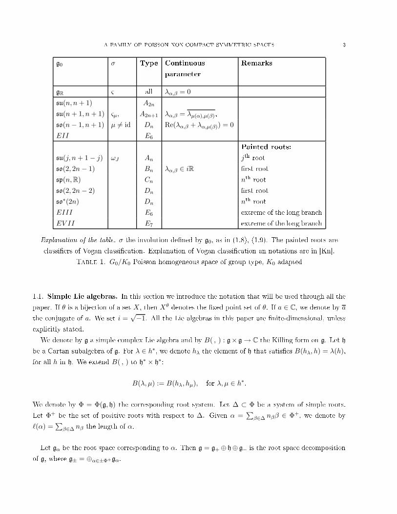
A FAMILY OF POISSON NON-COMPACT SYMMETRIC SPACES 3

g0 σ Type Continuous

parameter

Remarks

gR ς all λα,β = 0

su(n, n + 1) A2n

su(n + 1, n + 1) ςµ, A2n+1 λα,β = λµ(α),µ(β),

so(n − 1, n + 1) µ 6= id Dn Re(λα,β + λα,µ(β)) = 0

EII E6

Painted roots:

su(j, n + 1 − j) ωJ An jth root

so(2, 2n − 1) Bn λα,β ∈ iR rst root

sp(n, R) Cn nth root

so(2, 2n − 2) Dn rst root

so∗(2n) Dn nth root

EIII E6 extreme of the long bran h

EV II E7 extreme of the long bran h

Explanation of the table. σ the involution dened by g0, as in (1.8), (1.9). The painted roots are

lassiers of Vogan lassi ation. Explanation of Vogan lassi ation an notations are in [Kn.

Table 1. G0/K0 Poisson homogeneous spa e of group type, K0 adapted

1.1. Simple Lie algebras. In this se tion we introdu e the notation that will be used through all the

paper. If θ is a bije tion of a set X, then Xθdenotes the xed-point set of θ. If a ∈ C, we denote by a

the onjugate of a. We set i =√−1. All the Lie algebras in this paper are nite-dimensional, unless

expli itly stated.

We denote by g a simple omplex Lie algebra and by B( , ) : g× g → C the Killing form on g. Let h

be a Cartan subalgebra of g. For λ ∈ h∗, we denote hλ the element of h that satises B(hλ, h) = λ(h),

for all h in h. We extend B( , ) to h∗ × h∗:

B(λ, µ) := B(hλ, hµ), for λ, µ ∈ h∗.

We denote by Φ = Φ(g, h) the orresponding root system. Let ∆ ⊂ Φ be a system of simple roots.

Let Φ+be the set of positive roots with respe t to ∆. Given α =

∑β∈∆ nββ ∈ Φ+

, we denote by

ℓ(α) =∑

β∈∆ nβ the length of α.

Let gα be the root spa e orresponding to α. Then g = g+ ⊕ h⊕ g− is the root spa e de omposition

of g, where g± = ⊕α∈±Φ+gα.


We hoose root ve tors eα ∈ gα − 0 su h that

B(eα, e−α) = 1, for α ∈ Φ.(1.1)

Then

[eα, e−α] = hα,(1.2)

[eα, eβ ] = 0, if α + β 6= 0 and α + β 6∈ Φ.(1.3)

For every α, β ∈ Φ su h that α + β 6= 0, let Nα,β dened by

[eα, eβ ] = Nα,βeα+β , if α + β ∈ Φ.(1.4)

We set Nα,β = 0, if α+β 6= 0 and α+β 6∈ Φ. Thus, we have for all α, β and γ in Φ su h that α+β 6= 0,

Nα,β = −Nβ,α,(1.5)

Nα,β = Nβ,γ = Nγ,α, if α, β, γ ∈ Φ, α + β + γ = 0.(1.6)

The following fa t is well-known.

Lemma 1.1. Let α, β ∈ Φ su h that α + β ∈ Φ, and α − β 6∈ Φ. Then

(1.7) Nα,β N−α,−β = B(α, β)−1.

Proof. If we denote v = [eα, eβ ], then

[[eα, eβ], [e−α, e−β ]] = −[e−α, [e−β , v]] − [e−β, [v, e−α]],

[e−β, v] = −[eα, [eβ , e−β]] = −[eα, hβ ] = B(α, β)eα

[v, e−α] = −[[e−α, eα], eβ ] = −[h−α, eβ ] = B(α, β)eβ .

Set c = 1Nα,β N−α,−β

. Then

hα+β = [eα+β , e−α−β ] =1

Nα,β N−α,−β

[[eα, eβ ], [e−α, e−β ]]

= −c ([e−α, [e−β , v]] + [e−β , [v, e−α]]) = −cB(α, β)([e−α, eα] + [e−β , eβ ]) = cB(α, β)hα+β ,

and the result follows.

In the follows, trough all this work, g will denote a simple omplex Lie algebra and B( , ) the Killing

form orresponding to g. Also, h denotes a Cartan subalgebra of g, Φ = Φ(g, h) the orresponding

root system, ∆ a set of simple roots, Φ+the set of positive roots with respe t to ∆, gα the root spa e

orresponding to α ∈ Φ and g = g+ ⊕ h ⊕ g− the root spa e de omposition.


1.2. Absolutely simple real Lie algebras. We now des ribe the real Lie algebras we shall work

with. A nite-dimensional real Lie algebra is alled absolutely simple if its omplexi ation is a simple

omplex Lie algebra. It is well-known that a simple real Lie algebra is either absolutely simple or is

the reali ation of a omplex simple Lie algebra.

Let g be a simple omplex Lie algebra, h be a Cartan subalgebra, Φ be the root system and ∆ be

a system of simple roots. Let µ : ∆ → ∆ be an automorphism of the Dynkin diagram of order 1 or

2. We hoose eα ∈ gα − 0 su h that B(eα, e−α) = 1 for α ∈ Φ. Let J be any subset of the set ∆µ

of simple roots xed by µ; let χJ : ∆ → 0, 1 be the hara teristi fun tion of J . Then there exist

unique onjugate-linear Lie algebra involutions ςµ, ωµ,J of g given respe tively by

ςµ(eα) = eµ(α), ςµ(e−α) = e−µ(α),(1.8)

ωµ,J(eα) = (−1)χJ (α)e−µ(α), ωµ,J(e−α) = (−1)χJ (−α)eµ(α),(1.9)

for all α ∈ ∆. Ne essarily,

(1.10) ςµ(hα) = hµ(α), ωµ,J(hα) = −hµ(α).

We shall write

ς = ςid, ωJ = ωid,J , ω = ωid,∆.

Thus ω is the Chevalley involution of g, with respe t to h and ∆, and the xed point set of ω is a

ompa t form u0 of g. Sin e ω(eα) = −e−α for all α ∈ Φ see (1.14) below one has:

(1.11) u0 =∑

α∈Φ

R(i hα) +∑

α∈Φ

R(eα − e−α) +∑

α∈Φ

Ri (eα + e−α).

The following lemma a variation of [AJ, Lemma 2.1 will be useful later.

Lemma 1.2. Let σ : g → g be a onjugate-linear Lie algebra involution su h that σ(h) = h. Thus, we

an dene σ∗ : h∗ → h∗, the adjoint of σ, by σ∗(λ)(h) = λ(σ(h)), for λ ∈ H∗, h ∈ h. Then σ∗(Φ) = Φ

and σ(gα) = gσ∗(α), see lo . it. Then, there exists a hoi e of non-zero root ve tors eα ∈ gα, α ∈ Φ,

satisfying (1.1), su h that

(a). If σ∗(∆) = ∆, there exists a unique automorphism µ : ∆ → ∆ of the Dynkin diagram of order

1 or 2 (whi h does not depend on the hoi e of the eα's), su h that σ = ςµ and

ςµ(eα) = eµ(α),(1.12)

ςµ(hα) = hµ(α),(1.13)

for all α ∈ Φ, where µ : Φ → Φ is the linear extension of µ.


(b). If σ∗(∆) = −∆, the there exists a unique automorphism µ : ∆ → ∆ of the Dynkin diagram of

order 1 or 2 and a unique subset J of Φµ(neither µ nor J depend on the hoi e of the eα's) su h that:

σ = ωµ,J with J = J ∩ ∆. Furthermore,

ωµ,J(eα) = (−1)χJ(α)e−µ(α),(1.14)

ωµ,J(hα) = −hµ(α),(1.15)

for all α ∈ Φ, where µ : Φ → Φ is the linear extension of µ and χJ : Φ → 0, 1 the hara teristi

fun tion of J .

( ). Assume the situation in (b). Let α, β ∈ Φ and Nα,β be dened as in subse tion 1.1. We have

(1)

χJ(α) = χJ(−α) = χJ(µ(α)),(1.16)

(−1)χJ(α)+χ

J(β)N−µ(α),−µ(β) = (−1)χJ

(α+β)Nα,β.(1.17)

(2) Let χZJ : Φ → Z be the linear extension of χJ : ∆ → 0, 1. Then

(−1)χJ(α) = (−1)χZJ (α)+ℓ(α)+1

(1.18)

for all α ∈ Φ.

Proof. Assume that σ∗(∆) = ±∆. Let µ : ∆ → ∆ be given by µ = ±σ∗, a ording to the ase.

Then µ is an automorphism of the Dynkin diagram, and learly it has order 1 or 2. Let fα ∈ gα,

α ∈ Φ, be any hoi e of non-zero root ve tors satisfying B(fα, f−α) = 1. Let cα ∈ C − 0 be su h that

σ(fα) = cαfσ∗(α), α ∈ Φ. It is known that B(x, y) = B(σ(x), σ(y)) for all x, y ∈ g, see [H, p. 180.

Then, for all α ∈ Φ, we have 1 = B(fα, f−α) = B(σ(fα), σ(f−α)) = cαc−αB(fσ∗(α), f−σ∗(α)) = cαc−α.

Hen e, if α ∈ Φ, we have

cαc−α = 1.(1.19)

Now, fα = σ2(fα) = σ(cαfσ∗(α)) = cασ(fσ∗(α)) = cαcσ∗αfα, thus

cαcσ∗α = 1.(1.20)

We prove (a). In this ase σ∗ = µ. For α ∈ Φ+, dene dα, by cα = (dα)−1dµ(α). The existen e of

su h dα is lear. For α ∈ Φ let eα = dαfα, e−α = (dα)−1f−α. Then B(eα, e−α) = 1 and

σ(eα) = dαcα(dµ(α))−1eµ(α) = eµ(α), σ(e−α) = (dα)−1c−α(dµ(α))e−µ(α) = e−µ(α).

The se ond formula follows from (1.19). The uniqueness of µ is evident and (a) follows.


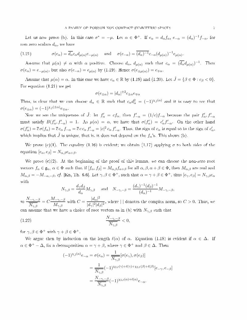
Let us now prove (b). In this ase σ∗ = −µ. Let α ∈ Φ+. If eα = dαfα, e−α = (dα)−1f−α, for

non-zero s alars dα, we have

(1.21) σ(eα) = dαcαdµ(α)e−µ(α) and σ(e−α) = (dα)−1c−α(dµ(α))−1eµ(α).

Assume that µ(α) 6= α with α positive. Choose dα, dµ(α) su h that cα = (dαdµ(α))−1. Then

σ(eα) = e−µ(α), but also σ(e−α) = eµ(α) by (1.19). Hen e σ(e±µ(α)) = e∓α.

Assume that µ(α) = α. In this ase we have cα ∈ R by (1.19) and (1.20). Let J = β ∈ Φ : cβ < 0.For equation (1.21) we get

σ(e±α) = |dα|±2c±αe∓α

Thus, is lear that we an hoose dα ∈ R su h that cαd2α = (−1)χJ

(α)and it is easy to see that

σ(e±α) = (−1)χJ(±α)e∓α.

Now we see the uniqueness of J : let f ′α = cfα, then f ′

−α = (1/c)f−α be ause the pair f ′α, f ′

−α

must satisfy B(f ′α, f ′

−α) = 1. As µ(α) = α, we have that σ(f ′α) = c′αf ′

−α. On the other hand

σ(f ′α) = c σ(fα) = c cα f−α = c c cα f ′

−α = |c|2 cα f ′−α. Thus, the sign of cα is equal to to the sign of c′α,

whi h implies that J is unique, that is, it does not depend on the fα's. This shows (b).

We prove ( )(1). The equality (1.16) is evident; we obtain (1.17) applying σ to both sides of the

equation [eα, eβ ] = Nα,βeα+β.

We prove ( )(2). At the beginning of the proof of this lemma, we an hoose the non-zero root

ve tors fα ∈ gα, α ∈ Φ su h that if [fα, fβ] = Mα,βfα+β for all α, β, α + β ∈ Φ, then Mα,β are real and

Mα,β = −M−α,−β, f. [Kn, Th. 6.6. Let γ, β ∈ Φ+, su h that α = γ + β ∈ Φ+

, thus [eγ , eβ] = Nγ,βeα

with

Nγ,β =dγdβ

dα

Mγ,β and N−γ,−β =(dγ)−1(dβ)−1

(dα)−1M−γ,−β,

so

N−γ,−β

Nγ,β

= CM−γ,−β

Mγ,β

with C =|dα|2

|dγ |2|dβ |2, where | | denotes the omplex norm, so C > 0. Thus, we

an assume that we have a hoi e of root ve tors as in (b) with Nγ,β su h that

(1.22)

N−γ,−β

Nγ,β

< 0,

for γ, β ∈ Φ+with γ + β ∈ Φ+

.

We argue then by indu tion on the length ℓ(α) of α. Equation (1.18) is evident if α ∈ ∆. If

α ∈ Φ+ − ∆, x a de omposition α = γ + β, where γ ∈ Φ+and β ∈ ∆. Then

(−1)χJ(α)e−α = σ(eα) =

1

Nγ,β

[σ(eγ), σ(eβ)]

=1

Nγ,β

(−1)χZJ (γ)+ℓ(γ)+χZJ (β)+ℓ(β)[e−γ , e−β ]

=N−γ,−β

Nγ,β

(−1)χZJ (α)+ℓ(α)e−α.


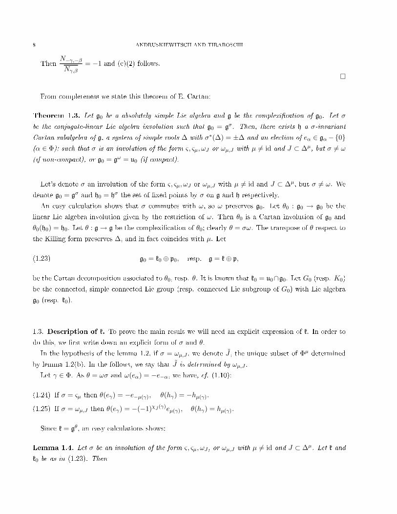
Then

N−γ,−β

Nγ,β

= −1 and ( )(2) follows.

From ompleteness we state this theorem of E. Cartan:

Theorem 1.3. Let g0 be a absolutely simple Lie algebra and g be the omplexi ation of g0. Let σ

be the onjugate-linear Lie algebra involution su h that g0 = gσ. Then, there exists h a σ-invariant

Cartan subalgebra of g, a system of simple roots ∆ with σ∗(∆) = ±∆ and an ele tion of eα ∈ gα −0(α ∈ Φ); su h that σ is an involution of the form ς, ςµ, ωJ or ωµ,J with µ 6= id and J ⊂ ∆µ

, but σ 6= ω

(if non- ompa t), or g0 = gω = u0 (if ompa t).

Let's denote σ an involution of the form ς, ςµ, ωJ or ωµ,J with µ 6= id and J ⊂ ∆µ, but σ 6= ω. We

denote g0 = gσand h0 = hσ

the set of xed points by σ on g and h respe tively.

An easy al ulation shows that σ ommutes with ω, so ω preserves g0. Let θ0 : g0 → g0 be the

linear Lie algebra involution given by the restri tion of ω. Then θ0 is a Cartan involution of g0 and

θ0(h0) = h0. Let θ : g → g be the omplexi ation of θ0; learly θ = σω. The transpose of θ respe t to

the Killing form preserves ∆, and in fa t oin ides with µ. Let

(1.23) g0 = k0 ⊕ p0, resp. g = k ⊕ p,

be the Cartan de omposition asso iated to θ0, resp. θ. It is known that k0 = u0∩g0. Let G0 (resp. K0)

be the onne ted, simple onne ted Lie group (resp. onne ted Lie subgroup of G0) with Lie algebra

g0 (resp. k0).

1.3. Des ription of k. To prove the main result we will need an expli it expression of k. In order to

do this, we rst write down an expli it form of σ and θ.

In the hypothesis of the lemma 1.2, if σ = ωµ,J , we denote J , the unique subset of Φµdetermined

by lemma 1.2(b). In the follows, we say that J is determined by ωµ,J .

Let γ ∈ Φ. As θ = ωσ and ω(eα) = −e−α, we have, f. (1.10):

If σ = ςµ then θ(eγ) = −e−µ(γ), θ(hγ) = −hµ(γ).(1.24)

If σ = ωµ,J then θ(eγ) = −(−1)χJ(γ)eµ(γ), θ(hγ) = hµ(γ).(1.25)

Sin e k = gθ, an easy al ulations shows:

Lemma 1.4. Let σ be an involution of the form ς, ςµ, ωJ , or ωµ,J with µ 6= id and J ⊂ ∆µ. Let k and

k0 be as in (1.23). Then


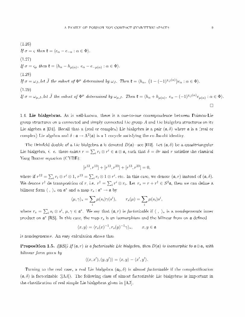
If σ = ς then k = 〈eα − e−α : α ∈ Φ〉.(1.26)

If σ = ςµ then k = 〈hα − hµ(α), eα − e−µ(α) : α ∈ Φ〉.(1.27)

If σ = ωJ , let J the subset of Φµdetermined by ωJ . Then k = 〈hα,

(1 − (−1)χJ

(α))eα : α ∈ Φ〉.

(1.28)

If σ = ωµ,J , let J the subset of Φµdetermined by ωµ,J . Then k = 〈hα + hµ(α), eα − (−1)χJ

(α)eµ(α) : α ∈ Φ〉.(1.29)

1.4. Lie bialgebras. As is well-known, there is a one-to-one orresponden e between Poisson-Lie

group stru tures on a onne ted and simply onne ted Lie group A and Lie bialgebra stru tures on its

Lie algebra a [D1. Re all that a (real or omplex) Lie bialgebra is a pair (a, δ) where a is a (real or

omplex) Lie algebra and δ : a → Λ2(a) is a 1- o y le satisfying the o-Ja obi identity.

The Drinfeld double of a Lie bialgebra a is denoted D(a) see [D2. Let (a, δ) be a quasitriangular

Lie bialgebra, i. e. there exists r =∑

i ri ⊗ ri ∈ a ⊗ a, su h that δ = ∂r and r satises the lassi al

Yang-Baxter equation (CYBE):

[r12, r13] + [r12, r23] + [r13, r23] = 0,

where if r12 =∑

i ri ⊗ ri ⊗ 1, r13 =∑

i ri ⊗ 1 ⊗ ri, et . In this ase, we denote (a, r) instead of (a, δ).

We denote r† de transposition of r, i.e. r† =∑

i ri ⊗ ri. Let rs = r + r† ∈ S2a, then we an dene a

bilinear form 〈 , 〉∗ on a∗ and a map rs : a∗ → a by

〈µ, γ〉∗ =∑

i

µ(si)γ(si), rs(µ) =∑

i

µ(si)si,

where rs =∑

i si ⊗ si, µ, γ ∈ a∗. We say that (a, r) is fa torizable if 〈 , 〉∗ is a nondegenerate inner

produ t on a∗ [RS. In this ase, the map rs is an isomorphism and the bilinear from on a dened

〈x, y〉 = 〈rs(x)−1, rs(y)−1γ〉∗, x, y ∈ a

is nondegenerate. An easy al ulation shows that

Proposition 1.5. ([RS) If (a, r) is a fa torizable Lie bialgebra, then D(a) is isomorphi to a⊕a, with

bilinear form given by

〈(x, x′), (y, y′)〉 = 〈x, y〉 − 〈x′, y′〉.

Turning to the real ase, a real Lie bialgebra (a0, δ) is almost fa torizable if the omplexi ation

(a, δ) is fa torizable ([AJ). The following lass of almost fa torizable Lie bialgebras is important in

the lassi ation of real simple Lie bialgebras given in [AJ.


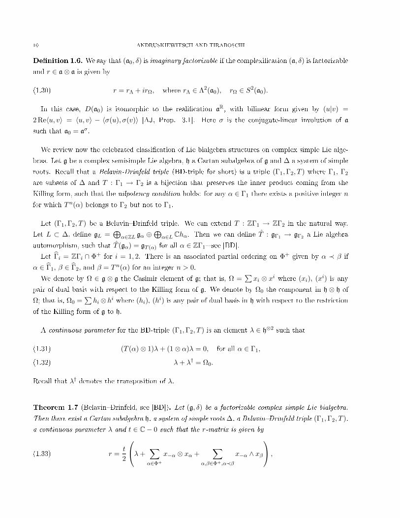
Denition 1.6. We say that (a0, δ) is imaginary fa torizable if the omplexi ation (a, δ) is fa torizable

and r ∈ a ⊗ a is given by

(1.30) r = rΛ + irΩ, where rΛ ∈ Λ2(a0), rΩ ∈ S2(a0).

In this ase, D(a0) is isomorphi to the reali ation aR, with bilinear form given by (u|v) =

2Re〈u, v〉 = 〈u, v〉 − 〈σ(u), σ(v)〉 [AJ, Prop. 3.1. Here σ is the onjugate-linear involution of a

su h that a0 = aσ.

We review now the elebrated lassi ation of Lie bialgebra stru tures on omplex simple Lie alge-

bras. Let g be a omplex semisimple Lie algebra, h a Cartan subalgebra of g and ∆ a system of simple

roots. Re all that a Belavin-Drinfeld triple (BD-triple for short) is a triple (Γ1,Γ2, T ) where Γ1, Γ2

are subsets of ∆ and T : Γ1 → Γ2 is a bije tion that preserves the inner produ t oming from the

Killing form, su h that the nilpoten y ondition holds: for any α ∈ Γ1 there exists a positive integer n

for whi h T n(α) belongs to Γ2 but not to Γ1.

Let (Γ1,Γ2, T ) be a BelavinDrinfeld triple. We an extend T : ZΓ1 → ZΓ2 in the natural way.

Let L ⊂ ∆, dene gL =⊕

α∈ZL gα ⊕ ⊕α∈L Chα. Then we an dene T : gΓ1

→ gΓ2a Lie algebra

automorphism, su h that T (gα) = gT (α) for all α ∈ ZΓ1 see [BD.

Let Γi = ZΓi ∩ Φ+for i = 1, 2. There is an asso iated partial ordering on Φ+

given by α ≺ β if

α ∈ Γ1, β ∈ Γ2, and β = T n(α) for an integer n > 0.

We denote by Ω ∈ g ⊗ g the Casimir element of g; that is, Ω =∑

xi ⊗ xiwhere (xi), (xi) is any

pair of dual basis with respe t to the Killing form of g. We denote by Ω0 the omponent in h ⊗ h of

Ω; that is, Ω0 =∑

hi ⊗hiwhere (hi), (hi) is any pair of dual basis in h with respe t to the restri tion

of the Killing form of g to h.

A ontinuous parameter for the BD-triple (Γ1,Γ2, T ) is an element λ ∈ h⊗2su h that

(T (α) ⊗ 1)λ + (1 ⊗ α)λ = 0, for all α ∈ Γ1,(1.31)

λ + λ† = Ω0.(1.32)

Re all that λ†denotes the transposition of λ.

Theorem 1.7 (BelavinDrinfeld, see [BD). Let (g, δ) be a fa torizable omplex simple Lie bialgebra.

Then there exist a Cartan subalgebra h, a system of simple roots ∆, a BelavinDrinfeld triple (Γ1,Γ2, T ),

a ontinuous parameter λ and t ∈ C − 0 su h that the r-matrix is given by

(1.33) r =t

2

λ +

∑

α∈Φ+

x−α ⊗ xα +∑

α,β∈Φ+,α≺β

x−α ∧ xβ

,


where xα ∈ gα are normalized by

B(xα, x−α) = 1, for all α ∈ Φ+(1.34)

T (xα) = xT (α), for all α ∈ Γ1.(1.35)

Clearly, r + r† = tΩ. Note that the normalization ondition (1.34) is the same as (1.1). Thus, given

any family eα : α ∈ Φ satisfying (1.1), there exists Cα ∈ C su h that

xα = Cαeα, CαC−α = 1.

We next re all some results of [AJ about the lassi ation of real simple Lie bialgebras. Let µ be

an automorphism of the Dynkin diagram.

• A BD-triple (Γ1,Γ2, T ) is µ-stable if µ(Γ1) = Γ1, µ(Γ2) = Γ2, and Tµ = µT .

• A BD-triple (Γ1,Γ2, T ) is µ-antistable if µ(Γ1) = Γ2, µ(Γ2) = Γ1, and T−1µ = µT .

If µ = id then all BD-triples are µ-stable, and the only BD-triple µ-antistable has Γ1 = Γ2 = ∅.

Proposition 1.8. Let (g0, δ) be an absolutely simple real Lie bialgebra. Let g be the omplexi ation

of g0 and let σ be the onjugate-linear involution of g whose xed-point set is g0. Assume that (g0, δ)

is almost fa torizable. Then there exist:

• A Cartan subalgebra h of g.

• A system of simple roots ∆ ⊂ Φ(g, h).

• A Belavin-Drinfeld triple (Γ1,Γ2, T ) and a ontinuous parameter λ ∈ h⊗2. Write

λ − λ† =∑

α,β∈∆

λα,βhα ∧ hβ.

By onvention λα,β = −λβ,α for all α, β ∈ ∆.

• A omplex number c with c2 ∈ R; set t = 2ic.

All these data verify:

(a) h is stable under σ (we denote h0 := h ∩ g0).

(b) σ∗(∆) is either ∆ or −∆; furthermore µ := σ∗ : ∆ → ±∆ is an automorphism of the Dynkin

diagram. There are two possibilities:

(i) If σ∗(∆) = ∆ then, by Lemma 1.2, there is an appropriate hoi e of the eα ∈ gα (α ∈ Φ)

satisfying (1.1), su h that σ is either ς or ςµ with µ 6= id and (1.12) holds.

If σ = ς, t ∈ R, then λα,β ∈ R for all α, β ∈ ∆ (no restri tions on the BD-triple).


If σ = ςµ, then t ∈ R, λα,β = λµ(α),µ(β), for all α, β ∈ ∆ and the BD-triple is µ-stable.

(ii) If σ∗(∆) = −∆ then, by Lemma 1.2, there is an appropriate hoi e of the eα ∈ gα (α ∈ Φ)

satisfying (1.1), su h that σ is either ωJ , ω or ωµ,J with µ 6= id and J ⊂ ∆µ, and (1.14) holds.

If σ = ωJ , or σ = ω, then t ∈ iR, λα,β ∈ iR, for all α, β ∈ ∆ and the BD-triple has

Γ1 = Γ2 = ∅.

If σ = ωµ,J , then t ∈ iR, λα,β = −λµ(α),µ(β), for all α, β ∈ ∆ and the BD-triple is µ-

antistable.

( ) δ = ∂r as in Theorem 1.7. Furthermore δ = ∂r0 where r0 ∈ Λ2(g0) is given by the formula

(1.36) r0 =t

2

λ − λ† +

∑

α∈Φ+

e−α ∧ eα +∑

α,β∈Φ+,α≺β

C−αCβ e−α ∧ eβ

,

with an adequate ele tion of Cα ∈ C for α ∈ Φ su h that CαC−α = 1.

(d)

(1.37) (θ ⊗ θ)r0 =t

2

∑

α,β∈∆

λα,βhα ∧ hβ −∑

α∈Φ+

e−α ∧ eα +∑

α,β∈Φ+,α≺β

C−αCβ eα ∧ e−β

.

Proof. Parts (a) to ( ) are [AJ, Lemma 3.1 and Lemma 3.4 ombined with Lemma 1.2. As r0 belongs

to Λ2(g0), (σ ⊗ σ)r0 = r0. Sin e θ = ωσ, part (d) follows.

1.5. Poisson homogeneous spa es of group type arising from graphs.

Let A be a onne ted and simply onne ted Poisson-Lie group with Lie bialgebra (a, δ). Let T be a

onne ted Lie subgroup of A with Lie algebra t. Re all that Poisson homogeneous stru tures on A/T

are lassied by Lagrangian subalgebras l of D(a) = a⊕a∗, the Drinfeld double of a, su h that l∩a = t

[D3.

Re all that the anoni al bilinear form of D(a) is given by 〈x+µ|x′+µ′〉 = µ′(x)+µ(x′) for x, x′ ∈ a,

µ, µ′ ∈ a∗. In this subse tion, if v is a subspa e of a, then v⊥ denotes the orthogonal subspa e with

respe t to 〈 | 〉, thus v⊥ ∩ a∗ = µ ∈ a∗ : µ(v) = 0 is the annihilator of v.

Lemma 1.9. If v is a subspa e of a, then u = v ⊕ (v⊥ ∩ a∗) is a Lagrangian subspa e of D(a).

Proof. Sin e v ⊂ a, v⊥ ∩ a∗ ⊂ a∗, and a, a∗ are isotropi , we have that v and v⊥ ∩ a∗ are isotropi .

As 〈v|v⊥ ∩ a∗〉 ⊂ 〈v|v⊥〉 = 0, u is isotropi . It remains to show that u is Lagrangian, or equivalently

that dim(u) = dim(a) =: n. Be ause of the non degenera y of the bilinear form on D(a) we have that

dim(v) + dim(v⊥) = dim(D(a)) = 2n. But v⊥ = a ⊕ (v⊥ ∩ a∗), thus dim(v⊥) = n + dim(v⊥ ∩ a∗).

Hen e dim(v) + dim(v⊥ ∩ a∗) = n.

The following result should be well-known; we give a proof for the sake of ompleteness.


Proposition 1.10. A/T is a Poisson homogeneous spa e of group type if and only if there exists a

Lagrangian subalgebra u of D(a) su h that

(1.38) u = t ⊕ (u ∩ a∗).

Note that (1.38) implies u ∩ a = t.

Proof. (⇒) Let u = t ⊕ (t⊥ ∩ a∗) ⊂ t⊥. It is lear that (1.38) holds, and u is a Lagrangian subspa e

by the previous Lemma. It remains to verify that u is a Lie subalgebra. Now, by hypothesis t and

t⊥ ∩ a∗ = µ ∈ a∗ : µ(t) = 0 are Lie subalgebras of D(a) (see the Introdu tion). Let x ∈ t, y ∈ t⊥ ∩ a∗

and z = [x, y]. If w ∈ t, 〈w|z〉 = 〈[w, x]|y〉 ∈ 〈t|t⊥〉 = 0. If w ∈ t⊥ ∩ a∗, 〈w|z〉 = −〈[w, y]|x〉 ∈〈t⊥ ∩ a∗|t〉 = 0. Thus 〈z|u〉 = 0. Sin e u is Lagrangian, we on lude that z ∈ u.

(⇐) If x ∈ t⊥ ∩ a∗, then 〈x|t〉 = 〈x|a∗〉 = 0, hen e 〈x|u〉 = 0. Thus 〈t⊥ ∩ a∗|u〉 = 0, and t⊥ ∩ a∗ ⊂ u

sin e u is Lagrangian. Hen e t ⊕ (t⊥ ∩ a∗) ⊂ u. By Lemma 1.9, t ⊕ (t⊥ ∩ a∗) is also a Lagrangian

subspa e. Then t ⊕ (t⊥ ∩ a∗) = u, and this implies that t⊥ ∩ a∗ = u ∩ a∗ is a Lie subalgebra of a∗.

The following onstru tion of Poisson homogeneous spa es was observed by C. De Con ini, and

independiently by Karolinsky [K. Let A be a onne ted (real or omplex) Poisson-Lie group with

fa torizable Lie bialgebra a: re all that the Drinfeld double is isomorphi to the Lie algebra a⊕ a, and

the invariant form is given by 〈(x, x′), (y, y′)〉 = 〈x, y〉 − 〈x′, y′〉 for (x, x′), (y, y′) ∈ a ⊕ a (Proposition

1.5). Let ρ ∈ Aut(a) preserving 〈 , 〉. Then, the graph of ρ, namely uρ = (x, ρ(x)) : x ∈ a, is a

Lagrangian subalgebra of the Drinfeld double and A/T is a Poisson homogeneous spa e, where T is

the onne ted omponent of the identity of Aρ.

This onstru tion an be extended to the imaginary-fa torizable ase. Let A0 be a onne ted real

Poisson-Lie group with imaginary fa torizable Lie bialgebra (a0, δ). Let a be the omplexi ation of

a0 and σ the onjugate-linear automorphism of a whose xed point set is a0. Let θ0 ∈ Aut(a0) su h

that θ := θ0 ⊗ id preserves 〈 , 〉. Let µ = θσ = σθ, a onjugate-linear automorphism of a. Let H be

the onne ted omponent of the identity of Aθ0

0 .

Proposition 1.11. Assume that θ0 is an involution. Then A0/H is a Poisson homogeneous spa e.

Proof. As a0 is imaginary fa torizable, re all that D(a0) is isomorphi to the reali ation aR, with

bilinear form given by (u|v) = 2Re〈u, v〉 = 〈u, v〉 − 〈σ(u), σ(v)〉 (see denition 1.6 and what follows).

We will show that the real Lie subalgebra m := (aR)µ is Lagrangian, so, from the Drinfeld's riterion,

A0/H results a Poisson homogeneous spa e. If u, v ∈ m, then (u|v) = 〈u, v〉 − 〈σ(u), σ(v)〉 = 〈u, v〉 −〈θ(u), θ(v)〉 = 0, thus m is isotropi . Sin e θσ = σθ, we have (aR)µ ∩ a0 = (aR)σθ ∩ a0 = a

θ0

0 . Also, m =

aθ0

0 ⊕ ip0, where p0 is the eigenspa e of θ0 of eigenvalue −1. Thus, dimm = dim aθ0

0 + dim p0 = dim a0,

sin e θ0 is an involution, and m is Lagrangian.

Note that this Poisson homogeneous spa e is of group type if and only if m = aθ0

0 ⊕ (m ∩ rs(a∗0)),

be ause of Proposition 1.10. For the denition de rs, see the beginning of subse tion 1.4 .


In on lusion, the symmetri spa es G0/K0 always bear a stru ture of Poisson homogeneous spa e,

by Propositions 1.8, 1.10 together with De Con ini's remark and 1.11. In this paper we shall

investigate when G0/K0 bears a stru ture of Poisson homogeneous spa e of group type.

2. Proof of the main result

In this se tion we x (g0, δ) an almost fa torizable absolutely simple real Lie bialgebra. Let G0 be a

non- ompa t absolutely simple real Lie group with nite enter and Lie algebra g0 and K0 de maximal

ompa t subgroup of G0 adapted to δ (see the introdu tion). As usual, k0 denotes the Lie algebra of

K0. Let σ be the onjugate-linear involution of g, the omplexi ation of g0, su h that g0 = gσ. Now

and at the end of this se tion we will use the notation of subse tion 1.2 and the notation and results of

proposition 1.8. Also, we use the des ription of k, the omplexi ation of k0, given in subse tion 1.3.

As we said in the Introdu tion, G0/K0 is a a Poisson homogeneous spa e of group type of G0 if and

only if k0 is a oideal of g0. Our goal is to determine when k0 is a oideal of g0.

Lemma 2.1. G0/K0 is a Poisson homogeneous spa e of group type if and only if

ad k0((id−θ) ⊗ (id−θ)(r0)

)= ad k

((id−θ)⊗ (id−θ)(r0)

)= 0.

Proof. Let r0 = r1 + r2 with r1 ∈ g0 ⊗ k0 + k0 ⊗ g0 and r2 ∈ p0 ⊗ p0. If u ∈ k0, then δ(u) = ad u r0 =

ad u r1 +ad ur2 and ad u r1 ∈∈ g0 ⊗ k0 + k0 ⊗ g0 and ad u r2 ∈ p0 ⊗ p0. Hen e k0 is a oideal if and only

if ad u r2 = 0 for all u ∈ k0. Now, if r1 =∑

xi⊗xiwith xi or xi

in k0 and r2 =∑

yi⊗yiwith yi and yi

in p0, be ause k0 a ts as id on k0 and as − id on p0, we have (id−θ)⊗ (id−θ)xi ⊗ xi = 0 for all i, and

(id−θ)⊗(id−θ)yi⊗yi = 4yi⊗yi. Thus (id−θ)⊗(id−θ)r0 = 4r2 and ad u (id−θ)⊗(id−θ)r0 = 4ad u r2.

Hen e k0 is a oideal if and only if ad u r2 = 0 for all u ∈ k0 if and only if ad u (id−θ) ⊗ (id−θ)r0 = 0

for all u ∈ k0 .

We next give an expli it expression of

r0 := (id−θ) ⊗ (id−θ)(r0) = r0 + (θ ⊗ θ)(r0) − (id⊗θ + θ ⊗ id)(r0)

a ording to the dierent possibilities for σ. Then we analyze when k0 is a oideal ase by ase.

2.1. Computation of (id−θ)⊗ (id−θ)(r0).

In the al ulations below, keep in mind the equality (f ⊗ id + id⊗f)(a ∧ b) = f(a) ∧ b + a ∧ f(b),

a, b ∈ V , f ∈ End V . Set

tα,β = 2Re(λα,β + λα,µ(β)), α, β ∈ ∆,(2.1)

sα,β = 2 i Im(λα,β − λα,µ(β)), α, β ∈ ∆,(2.2)

dα,β = C−αCβ , α, β ∈ Φ+, α ≺ β.(2.3)


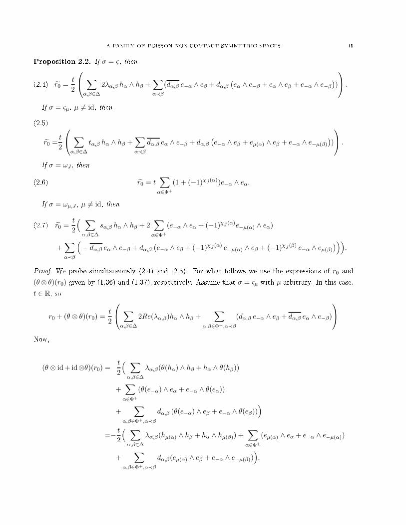
Proposition 2.2. If σ = ς, then

r0 =t

2

∑

α,β∈∆

2λα,β hα ∧ hβ +∑

α≺β

(dα,β e−α ∧ eβ + dα,β

(eα ∧ e−β + eα ∧ eβ + e−α ∧ e−β

))

.(2.4)

If σ = ςµ, µ 6= id, then

r0 =t

2

∑

α,β∈∆

tα,β hα ∧ hβ +∑

α≺β

dα,β eα ∧ e−β + dα,β

(e−α ∧ eβ + eµ(α) ∧ eβ + e−α ∧ e−µ(β)

))

.

(2.5)

If σ = ωJ , then

(2.6) r0 = t∑

α∈Φ+

(1 + (−1)χJ(α))e−α ∧ eα.

If σ = ωµ,J , µ 6= id, then

(2.7) r0 =t

2

( ∑

α,β∈∆

sα,β hα ∧ hβ + 2∑

α∈Φ+

(e−α ∧ eα + (−1)χJ(α)e−µ(α) ∧ eα)

+∑

α≺β

(− dα,β eα ∧ e−β + dα,β

(e−α ∧ eβ + (−1)χJ

(α) e−µ(α) ∧ eβ + (−1)χJ(β) e−α ∧ eµ(β)

))).

Proof. We probe simultaneously (2.4) and (2.5). For what follows we use the expressions of r0 and

(θ⊗ θ)(r0) given by (1.36) and (1.37), respe tively. Assume that σ = ςµ with µ arbitrary. In this ase,

t ∈ R, so

r0 + (θ ⊗ θ)(r0) =t

2

∑

α,β∈∆

2Re(λα,β)hα ∧ hβ +∑

α,β∈Φ+,α≺β

(dα,β e−α ∧ eβ + dα,β eα ∧ e−β)

Now,

(θ ⊗ id + id⊗θ)(r0) =t

2

( ∑

α,β∈∆

λα,β(θ(hα) ∧ hβ + hα ∧ θ(hβ))

+∑

α∈Φ+

(θ(e−α) ∧ eα + e−α ∧ θ(eα))

+∑

α,β∈Φ+,α≺β

dα,β (θ(e−α) ∧ eβ + e−α ∧ θ(eβ)))

=− t

2

( ∑

α,β∈∆

λα,β(hµ(α) ∧ hβ + hα ∧ hµ(β)) +∑

α∈Φ+

(eµ(α) ∧ eα + e−α ∧ e−µ(α))

+∑

α,β∈Φ+,α≺β

dα,β(eµ(α) ∧ eβ + e−α ∧ e−µ(β))).


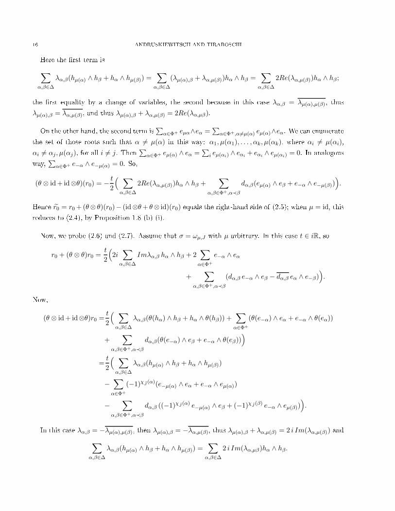
Here the rst term is

∑

α,β∈∆

λα,β(hµ(α) ∧ hβ + hα ∧ hµ(β)) =∑

α,β∈∆

(λµ(α),β + λα,µ(β))hα ∧ hβ =∑

α,β∈∆

2Re(λα,µ(β))hα ∧ hβ ;

the rst equality by a hange of variables, the se ond be ause in this ase λα,β = λµ(α),µ(β), thus

λµ(α),β = λα,µ(β), and thus λµ(α),β + λα,µ(β) = 2Re(λα,µβ).

On the other hand, the se ond term is

∑α∈Φ+ eµα∧eα =

∑α∈Φ+,α6=µ(α) eµ(α)∧eα. We an enumerate

the set of those roots su h that α 6= µ(α) in this way: α1, µ(α1), . . . , αk, µ(αk), where αi 6= µ(αi),

αi 6= αj, µ(αj), for all i 6= j. Then∑

α∈Φ+ eµ(α) ∧ eα =∑

i eµ(αi) ∧ eαi+ eαi

∧ eµ(αi) = 0. In analogous

way,

∑α∈Φ+ e−α ∧ e−µ(α) = 0. So,

(θ ⊗ id + id⊗θ)(r0) = − t

2

( ∑

α,β∈∆

2Re(λα,µ(β))hα ∧ hβ +∑

α,β∈Φ+,α≺β

dα,β(eµ(α) ∧ eβ + e−α ∧ e−µ(β))).

Hen e r0 = r0 + (θ⊗ θ)(r0)− (id⊗θ + θ⊗ id)(r0) equals the right-hand side of (2.5); when µ = id, this

redu es to (2.4), by Proposition 1.8 (b) (i).

Now, we probe (2.6) and (2.7). Assume that σ = ωµ,J with µ arbitrary. In this ase t ∈ iR, so

r0 + (θ ⊗ θ)r0 =t

2

(2i

∑

α,β∈∆

Imλα,β hα ∧ hβ + 2∑

α∈Φ+

e−α ∧ eα

+∑

α,β∈Φ+,α≺β

(dα,β e−α ∧ eβ − dα,β eα ∧ e−β)).

Now,

(θ ⊗ id + id⊗θ)r0 =t

2

( ∑

α,β∈∆

λα,β(θ(hα) ∧ hβ + hα ∧ θ(hβ)) +∑

α∈Φ+

(θ(e−α) ∧ eα + e−α ∧ θ(eα))

+∑

α,β∈Φ+,α≺β

dα,β(θ(e−α) ∧ eβ + e−α ∧ θ(eβ)))

=t

2

( ∑

α,β∈∆

λα,β(hµ(α) ∧ hβ + hα ∧ hµ(β))

−∑

α∈Φ+

(−1)χJ(α)(e−µ(α) ∧ eα + e−α ∧ eµ(α))

−∑

α,β∈Φ+,α≺β

dα,β ((−1)χJ(α) e−µ(α) ∧ eβ + (−1)χJ

(β) e−α ∧ eµ(β))).

In this ase λα,β = −λµ(α),µ(β), then λµ(α),β = −λα,µ(β), thus λµ(α),β + λα,µ(β) = 2 i Im(λα,µ(β)) and

∑

α,β∈∆

λα,β(hµ(α) ∧ hβ + hα ∧ hµ(β)) =∑

α,β∈∆

2 i Im(λα,µβ)hα ∧ hβ.


Now the se ond term is

∑

α∈Φ+

(−1)χJ(α)(e−µ(α) ∧ eα + e−α ∧ eµ(α)) = 2

∑

α∈Φ+

(−1)χJ(α) e−µ(α) ∧ eα.

Thus

(θ ⊗ id + id⊗θ)(r0) =t

2

(2i

∑

α,β∈∆

Im(λα,µβ)hα ∧ hβ − 2∑

α∈Φ+

(−1)χJ(α) e−µ(α) ∧ eα

−∑

α,β∈Φ+,α≺β

dα,β ((−1)χJ(α) e−µ(α) ∧ eβ + (−1)χJ

(β) e−α ∧ eµ(β))).

Hen e r0 = r0 +(θ⊗ θ)(r0)−((id⊗θ)+ (θ⊗ id)

)(r0) equals the right-hand side of (2.7). When µ = id,

this redu es to (2.6); indeed re all that Γ1 = Γ2 = ∅ in this ase by [AJ.

2.2. Case σ = ςµ, Γ1 = Γ2 = ∅. We begin with arbitrary µ. Re all the denition of tα,β in (2.1).

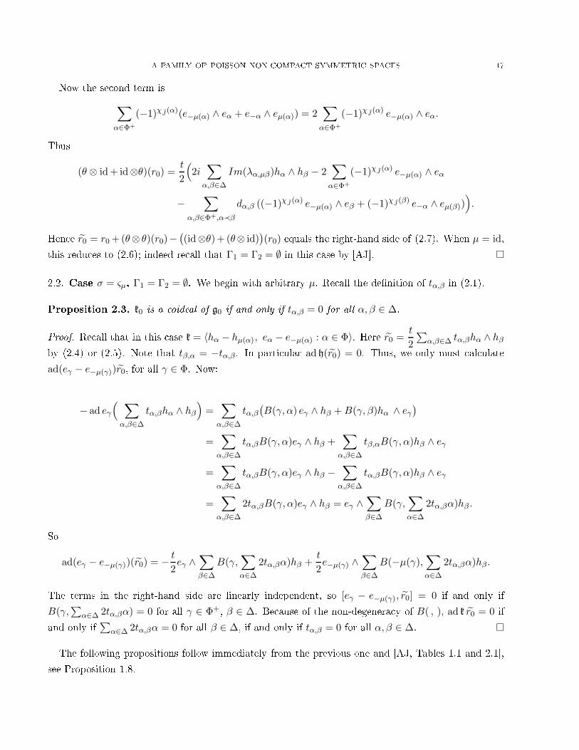
Proposition 2.3. k0 is a oideal of g0 if and only if tα,β = 0 for all α, β ∈ ∆.

Proof. Re all that in this ase k = 〈hα − hµ(α), eα − e−µ(α) : α ∈ Φ〉. Here r0 =t

2

∑α,β∈∆ tα,βhα ∧ hβ

by (2.4) or (2.5). Note that tβ,α = −tα,β. In parti ular ad h(r0) = 0. Thus, we only must al ulate

ad(eγ − e−µ(γ))r0, for all γ ∈ Φ. Now:

− ad eγ

( ∑

α,β∈∆

tα,βhα ∧ hβ

)=

∑

α,β∈∆

tα,β

(B(γ, α) eγ ∧ hβ + B(γ, β)hα ∧ eγ

)

=∑

α,β∈∆

tα,βB(γ, α)eγ ∧ hβ +∑

α,β∈∆

tβ,αB(γ, α)hβ ∧ eγ

=∑

α,β∈∆

tα,βB(γ, α)eγ ∧ hβ −∑

α,β∈∆

tα,βB(γ, α)hβ ∧ eγ

=∑

α,β∈∆

2tα,βB(γ, α)eγ ∧ hβ = eγ ∧∑

β∈∆

B(γ,∑

α∈∆

2tα,βα)hβ .

So

ad(eγ − e−µ(γ))(r0) = − t

2eγ ∧

∑

β∈∆

B(γ,∑

α∈∆

2tα,βα)hβ +t

2e−µ(γ) ∧

∑

β∈∆

B(−µ(γ),∑

α∈∆

2tα,βα)hβ .

The terms in the right-hand side are linearly independent, so [eγ − e−µ(γ), r0] = 0 if and only if

B(γ,∑

α∈∆ 2tα,βα) = 0 for all γ ∈ Φ+, β ∈ ∆. Be ause of the non-degenera y of B( , ), ad k r0 = 0 if

and only if

∑α∈∆ 2tα,βα = 0 for all β ∈ ∆, if and only if tα,β = 0 for all α, β ∈ ∆.

The following propositions follow immediately from the previous one and [AJ, Tables 1.1 and 2.1,

see Proposition 1.8.


Proposition 2.4. If σ = ς and Γ1 = Γ2 = ∅, then k0 is a oideal of g0 if and only if λα,β = 0 for all

α, β ∈ ∆.

Proposition 2.5. If σ = ςµ with µ 6= id and Γ1 = Γ2 = ∅, then k0 is a oideal of g0 if and only if the

ontinuous parameter λ satises λα,β = λµ(α),µ(β) and tα,β = 0, for all α, β ∈ ∆.

2.3. Case σ = ςµ, Γ1 6= ∅, Γ2 6= ∅. For arbitrary µ, we have:

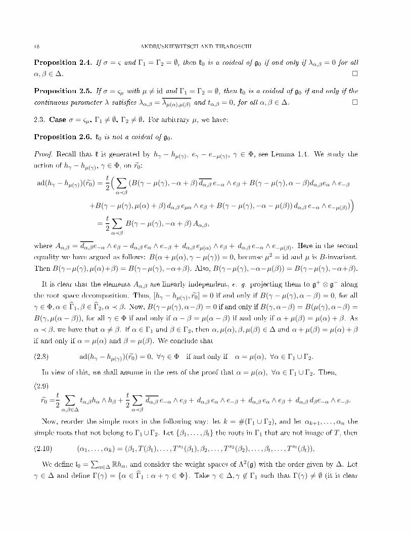
Proposition 2.6. k0 is not a oideal of g0.

Proof. Re all that k is generated by hγ − hµ(γ), eγ − e−µ(γ), γ ∈ Φ, see Lemma 1.4. We study the

a tion of hγ − hµ(γ), γ ∈ Φ, on r0:

ad(hγ − hµ(γ))(r0) =t

2

( ∑

α≺β

(B(γ − µ(γ),−α + β) dα,β e−α ∧ eβ + B(γ − µ(γ), α − β)dα,βeα ∧ e−β

+B(γ − µ(γ), µ(α) + β) dα,β eµα ∧ eβ + B(γ − µ(γ),−α − µ(β)) dα,β e−α ∧ e−µ(β)))

=t

2

∑

α≺β

B(γ − µ(γ),−α + β)Aα,β ,

where Aα,β = dα,βe−α ∧ eβ − dα,β eα ∧ e−β + dα,β eµ(α) ∧ eβ + dα,β e−α ∧ e−µ(β). Here in the se ond

equality we have argued as follows: B(α + µ(α), γ − µ(γ)) = 0, be ause µ2 = id and µ is B-invariant.

Then B(γ−µ(γ), µ(α)+β) = B(γ−µ(γ),−α+β). Also, B(γ−µ(γ),−α−µ(β)) = B(γ−µ(γ),−α+β).

It is lear that the elements Aα,β are linearly independent, e. g. proje ting them to g+ ⊗ g− along

the root spa e de omposition. Thus, [hγ − hµ(γ), r0] = 0 if and only if B(γ − µ(γ), α − β) = 0, for all

γ ∈ Φ, α ∈ Γ1, β ∈ Γ2, α ≺ β. Now, B(γ−µ(γ), α−β) = 0 if and only if B(γ, α−β) = B(µ(γ), α−β) =

B(γ, µ(α − β)), for all γ ∈ Φ if and only if α − β = µ(α − β) if and only if α + µ(β) = µ(α) + β. As

α ≺ β, we have that α 6= β. If α ∈ Γ1 and β ∈ Γ2, then α, µ(α), β, µ(β) ∈ ∆ and α + µ(β) = µ(α) + β

if and only if α = µ(α) and β = µ(β). We on lude that

(2.8) ad(hγ − hµ(γ))(r0) = 0, ∀γ ∈ Φ if and only if α = µ(α), ∀α ∈ Γ1 ∪ Γ2.

In view of this, we shall assume in the rest of the proof that α = µ(α), ∀α ∈ Γ1 ∪ Γ2. Then,

r0 =t

2

∑

α,β∈∆

tα,βhα ∧ hβ +t

2

∑

α≺β

dα,β e−α ∧ eβ + dα,β eα ∧ e−β + dα,β eα ∧ eβ + dα,β dβe−α ∧ e−β .

(2.9)

Now, reorder the simple roots in the following way: let k = #(Γ1 ∪ Γ2), and let αk+1, . . . , αn the

simple roots that not belong to Γ1 ∪Γ2. Let β1, . . . , βt the roots in Γ1 that are not image of T , then

(2.10) (α1, . . . , αk) = (β1, T (β1), . . . , Ts1(β1), β2, . . . , T

s2(β2), . . . , βt, . . . , Tst(βt)),

We dene l0 =∑

α∈∆ Rhα, and onsider the weight spa es of Λ2(g) with the order given by ∆. Let

γ ∈ ∆ and dene Γ(γ) = α ∈ Γ1 : α + γ ∈ Φ. Take γ ∈ ∆, γ 6∈ Γ1 su h that Γ(γ) 6= ∅ (it is lear


that su h γ exists, otherwise g would be of type A1 and in this ase Γ1 = Γ2 = ∅). Take γ1 in Γ(γ)

and γ2 ∈ Γ2 su h that γ1 ≺ γ2. We will prove that the weight γ1 + γ2 + γ o urs in [eγ − dγe−µγ , r0],

so the last one is not zero. Now,

(2.11) [eγ , eγ1∧ eγ2

] = Nγ,γ1eγ+γ1

∧ eγ2+ Nγ,γ2

eγ1∧ eγ+γ2

,

and, at least, the rst term is not 0, be ause γ1 ∈ Γ(γ). We will see that the term eγ+γ1∧ eγ2

is not

an elled by the other terms of [eγ − dγe−µγ , r0], that are of the form:

[eγ , eγ′

1∧ eγ′

2] =Nγ,γ′

1eγ+γ′

1∧ eγ′

2+ Nγ,γ′

2eγ′

1∧ eγ+γ′

2,(2.12)

[eγ , e−γ′

1∧ eγ′

2] =Nγ,−γ′

1eγ−γ′

1∧ eγ′

2+ Nγ,γ′

2e−γ′

1∧ eγ+γ′

2,(2.13)

[eγ , eγ′

1∧ e−γ′

2] =Nγ,γ′

1eγ+γ′

1∧ e−γ′

2+ Nγ,−γ′

2eγ′

1∧ eγ−γ′

2,(2.14)

[eγ , e−γ′

1∧ e−γ′

2] =Nγ,−γ′

1eγ−γ′

1∧ e−γ′

2+ Nγ,−γ′

2e−γ′

1∧ eγ−γ′

2,(2.15)

[e−µ(γ), eγ′

1∧ eγ′

2] =N−µ(γ),γ′

1e−µ(γ)+γ′

1∧ eγ′

2+ N−µ(γ),γ′

2eγ′

1∧ e−µ(γ)+γ′

2,(2.16)

[e−µ(γ), e−γ′

1∧ eγ′

2] =N−µ(γ),−γ′

1e−µ(γ)−γ′

1∧ eγ′

2+ N−µ(γ),γ′

2e−γ′

1∧ e−µ(γ)+γ′

2,(2.17)

[e−µ(γ), eγ′

1∧ e−γ′

2] =N−µ(γ),γ′

1e−µ(γ)+γ′

1∧ e−γ′

2+ N−µ(γ),−γ′

2eγ′

1∧ e−µ(γ)−γ′

2,(2.18)

[e−µ(γ), e−γ′

1∧ e−γ′

2]=N−µ(γ),−γ′

1e−µ(γ)−γ′

1∧ e−γ′

2+ N−µ(γ),−γ′

2e−γ′

1∧ e−µ(γ)−γ′

2,(2.19)

It is lear that eγ+γ1∧eγ2

annot be an elled with terms of type (2.13), (2.14), (2.15), (2.17), (2.18)

and (2.19) be ause of there are negative roots in the fa tors of the terms of the RHS of these equations

(re all that γ and µ(γ) are simple).

It ould be an elation between a term of (2.12) and eγ+γ1∧ eγ2

if

(a) γ1 + γ = γ′1 + γ and γ2 = γ′

2, or

(b) γ1 + γ = γ′2 and γ2 = γ′

1 + γ, or

( ) γ1 + γ = γ′1 and γ2 = γ′

2 + γ, or

(d) γ1 + γ = γ′2 + γ and γ2 = γ′

1.

Now, (a) ould be satised if and only if γ1 = γ′1 and γ2 = γ′

2. In the ase (b) we have that γ1 +γ = γ′2,

thus γ ∈ Γ2. As γ1 ≺ γ2 and γ′1 ≺ γ′

2, there exist k, s ∈ N su h that T k(γ1) = γ2 = γ′1 + γ and

T s(γ′1) = γ′

2 = γ1+γ. If we think in terms of the base (2.10) it is easy to see that the last two equalities

an not happen simultaneously. The ase ( ) results in a ontradi tion be ause γ1 + γ = γ′1 implies

that γ belongs to Γ1. Finally, in the ase (d) we have that T k(γ1) = γ2 = γ′1 and T s(γ′

1) = γ′2 = γ1,

thus T k+s(γ1) = γ1, whi h ontradi ts the nilpoten y of T .

Now, it ould be an ellation between a term of (2.16) and eγ+γ1∧ eγ2

if

(a) γ1 + γ = γ′1−µ(γ) and γ2 = γ′

2, or

(b) γ1 + γ = γ′2 and γ2 = γ′

1−µ(γ), or

( ) γ1 + γ = γ′1 and γ2 = γ′

2−µ(γ), or

(d) γ1 + γ = γ′2−µ(γ) and γ2 = γ′

1.


In the ase (a), as γ and µ(γ) not belongs to Γ1, we have that γ′1 − µ(γ) is not a root, a ontradi tion

be ause γ′1 − µ(γ) = γ1 + γ. In (b), as γ′

1−µ(γ) = γ2 is a root, we have that µ(γ) is in Γ1, thus γ is

in Γ1, a ontradi tion. In ( ), γ1 + γ = γ′1 implies that γ ∈ Γ1, a ontradi tion. In (d), if γ 6= µ(γ),

and in onsequen e γ, µ(γ) 6∈ Γ1 ∪ Γ2, we have that γ1 + γ + µ(γ) = γ′2, thus γ ∈ Γ2, a ontradi tion.

Thus γ = µ(γ) and we have γ1 + γ = γ′2−γ and γ2 = γ′

1. Now, T k(γ1) = γ2 = γ′1 and T s(γ′

1) = γ′2, so

T k+s(γ1) = γ′2 = γ1 + 2γ. If we think in terms of the base (2.10) it is easy to see that the last equality

an not happen.

2.4. Case σ = ωJ . In this ase ne essarily Γ1 = Γ2 = ∅. See Proposition 1.8.

Proposition 2.7. If k0 is oideal of g0 then #J = #∆ − 1; say α = ∆ − J . Assuming this, k0 is

oideal of g0 if and only if the oe ient of α in the largest root of Φ is 1. This happens if and only if

(1) g0 is of type An and α ∈ ∆ is arbitrary, or

(2) g0 is of type Bn and α is the leftmost extreme of the Dynkin diagram (α is the shortest simple

root), or

(3) g0 is of type Cn and α is the rightmost extreme of the Dynkin diagram (α is the longest simple

root), or

(4) g0 is of type Dn and α is an extreme of the Dynkin diagram, or

(5) g0 is of type E6 and α is extreme of the long bran h of the Dynkin diagram, or

(6) g0 is of type E7 and α is the extreme of the long bran h of the Dynkin diagram.

Proof. Let us assume that σ = ωJ . Re all from (2.6) that

r0 = t∑

α∈Φ+

(1 + (−1)χJ(α))e−α ∧ eα.

Step 1. [hγ , r0] = 0 for all γ ∈ ∆.

This is evident. Next, we ompute:

Step 2. If γ ∈ Φ+, then

ad eγ(r0) = t((1 + (−1)χJ

(γ))hγ ∧ eγ +∑

α∈Φ+,γ−α∈Φ+

(1 + (−1)χJ(α))Nγ,−α eγ−α ∧ eα(2.20)

+ (1 + (−1)χJ(γ))

∑

α∈Φ+,γ+α∈Φ+

Nγ,−α(−1)χJ(α) e−α ∧ eγ+α

),

ad e−γ(r0) = t(− (1 + (−1)χJ

(γ))e−γ ∧ hγ +∑


(1 + (−1)χJ(α))N−γ,α e−α ∧ eα−γ(2.21)

− (1 + (−1)χJ(γ))

∑

α∈Φ+,α−γ∈Φ+

N−γ,α(−1)χJ(α−γ) e−α ∧ e−γ+α

).


Proof. Clearly,

ad eγ(r0) = t∑

α∈Φ+,α6=γ

(1 + (−1)χJ(α))

(Nγ,−αeγ−α ∧ eα + Nγ,αe−α ∧ eγ+α

)+ t(1 + (−1)χJ

(γ))hγ ∧ eγ .

Sin e γ ∈ Φ+, we have

∑

α∈Φ+,α6=γ

(1 + (−1)χJ(α))


)

=∑


(1 + (−1)χJ(α))Nγ,−αeγ−α ∧ eα

+∑

α∈Φ+,γ−α∈Φ−

(1 + (−1)χJ(α))Nγ,−αeγ−α ∧ eα

+∑


(1 + (−1)χJ(α))Nγ,αe−α ∧ eγ+α

=∑


(1 + (−1)χJ(α))Nγ,−αeγ−α ∧ eα

+∑


[(1 + (−1)χJ

(α+γ))Nγ,−α−γ + (1 + (−1)χJ(α))Nγ,α

]e−α ∧ eγ+α.

Now, (−1)χJ(α+γ) = −(−1)χJ

(α)(−1)χJ(γ)

; and Nγ,α = N−α−γ,γ = −Nγ,−α−γ by (1.5) and (1.6).

Thus the se ond sum in the last expression equals

∑


Nγ,α(−1)χJ(α)(1 + (−1)χJ

(γ))e−α ∧ eγ+α,

and (2.20) follows. The proof of (2.21) is ompletely analogous.

Step 3. k0 is a oideal of g0 if and only if for any γ ∈ Φ+su h that (−1)χJ

(γ) = −1, and for any

α, β ∈ Φ+su h that γ = α + β, one has (−1)χJ

(α) = (−1)χJ(β) = −1.

Proof. By Lemma 2.1 (1.28) and Step 1, k0 is a oideal of g0 if and only if

(1− (−1)χJ

(γ))ad eγ(r0) = 0

for all γ ∈ Φ. If (−1)χJ(γ) = 0, then there is nothing to prove. If γ ∈ Φ+

and (−1)χJ(γ) = 1, then by

(2.20) we have

(1 − (−1)χJ

(γ))ad eγ(r0) = 2t

∑


(1 + (−1)χJ(α))Nγ,−α eγ−α ∧ eα.

Let α1, . . . , αr ∈ Φ+a maximal set satisfying β1 := γ − α1, . . . , βr := γ − αr ∈ Φ+

and αi 6= βj for all

i, j. Then the last equation is equivalent to:

(1 − (−1)χJ

(γ))ad eγ(r0) = 2t

r∑

i=1

(1 + (−1)χJ(αi))Nγ,−αi

eβi∧ eαi

+ (1 + (−1)χJ(βi))Nγ,−βi

eαi∧ eβi

.

From (1.5) and (1.6) we have

Nγ,−αi= N−βi,γ = −Nγ,−β1

,


thus

(1 − (−1)χJ

(γ))ad eγ(r0) = 2t

r∑

i=1

(1 + (−1)χJ(αi))Nγ,−αi

eβi∧ eαi

+ (1 + (−1)χJ(βi))(−Nγ,−αi

) eαi∧ eβi

= 2tr∑

i=1

(2 + (−1)χJ(αi) + (−1)χJ

(βi))Nγ,−αieβi

∧ eαi.

Then

(1−(−1)χJ

(γ))ad eγ(r0) = 0 if and only if (−1)χJ

(α) = −1 for all α ∈ Φ+su h that γ−α ∈ Φ+

.

This proves the laim.

Step 4. If k0 is a oideal of g0 then #J = #∆ − 1.

Proof. If J = ∆ then g0 is ompa t, ontrary to our assumptions. Thus there is at least one element

in ∆ − J . Assume that there is more than one element in ∆ − J . We an then hoose α 6= β ∈ ∆ − J

su h that the minimal path from α to β in the Dynkin diagram ontains only points in J . It follows

that there exists γ ∈ Φ+satisfying

γ = α + k1α1 + · · · + ksαs + β,

with α1, . . . , αs ∈ J and α + k1α1 + · · · + ksαs ∈ Φ+. Then, by Lemma 1.2 ( ):

(−1)χJ(γ) = (−1)χZJ (γ)+ℓ(γ)+1 = (−1)2k1+···+2ks+1 = −1,

but β /∈ J , ontradi ting Step 3.

Step 5. Assume that ∆ − J = α. If γ ∈ Φ+, write γ =

∑β∈∆ kββ. Then k0 is oideal of g0 if and

only if the oe ient kα is 0 or 1 for any γ ∈ Φ+.

Proof. Assume that k0 is a oideal of g0. If for some γ ∈ Φ+, kα ≥ 2 then we an assume that kα = 2

(for some other positive root, say). Computing (−1)χJ(γ)

as in the previous step we get a ontradi tion.

Conversely, assume that the oe ient kα is 0 or 1 for any γ ∈ Φ+. Note that (−1)χJ

(γ) = −(−1)kα.

Thus (−1)χJ(γ) = −1 if and only if kα = 0. We on lude now from Step 3.

Re all that the largest root of Φ is the highest weight of the adjoint representation of g.

Step 6. Assume that ∆ − J = α. Then k0 is oideal of g0 if and only if the oe ient of α in the

largest root of Φ is 1.

Proof. If

∑β∈∆ tββ is the largest root and γ =

∑β∈∆ kββ ∈ Φ+

, then kβ ≤ tβ. Thus the Step follows

immediately from Step 5.

It remains only to determine the Dynkin diagrams with a simple root whose oe ient in the largest

root is 1. This is an easy task, by inspe ting the largest root of ea h system as listed in [Kn, Appendix

C. For example, the largest root orresponding to a system of type Bn is α1 +∑n

i=2 2αi. So, from


Step 6, k0 is sub oideal of g0 if and only if α = α1. The same argument applies to the other Dynkin

diagrams.

2.5. Case σ = ωµ,J , µ 6= id, Γ1 = Γ2 = ∅. We shall show that k0 is not oideal of g0 ex ept for g0 of

type A2. We begin by the following redu tion; re all the set J dened in Lemma 1.2.

Lemma 2.8. If γ ∈ Φ+then ad(eγ − (−1)χJ

(γ)eµ(γ))(r0) ≡ tuγ mod h ⊗ g + g ⊗ h, where

uγ =∑


Nγ,−αeγ−α ∧ eα

+∑


(−1)χJ(γ)+1Nµ(γ),−µ(α)eµ(γ−α) ∧ eµ(α)

+∑


(−1)χJ(α)(Nγ,−α − N−γ,α)eγ−α ∧ eµ(α)

+∑


(−1)χJ(γ+α)(Nα,γ + N−α,−γ)e−α ∧ eµ(γ+α)

+∑


(−1)χJ(α)(Nγ,α + N−γ,−α)e−µ(α) ∧ eγ+α

Proof. For shortness, let “X ≡ Y ” mean “X ≡ Y mod h ⊗ g + g ⊗ h”. We ompute:

1

tad eγ(r0) ≡

∑

α∈Φ+

([eγ , e−α] ∧ eα + e−α ∧ [eγ , eα] + (−1)χJ

(α)([eγ , e−µ(α)] ∧ eα + e−µ(α) ∧ [eγ , eα]

))

≡∑

α∈Φ+,α6=γ


)

+∑

α∈Φ+,α6=µ(γ)

(−1)χJ(α)Nγ,−µ(α)eγ−µ(α) ∧ eα

+∑

α∈Φ+

(−1)χJ(α)Nγ,αe−µ(α) ∧ eγ+α

≡∑


Nγ,−αeγ−α ∧ eα(A)

+∑

α∈Φ+,α−µ(γ)∈Φ+

(−1)χJ(α)Nγ,−µ(α)eγ−µ(α) ∧ eα(B)

+∑

α∈Φ+,µ(γ)−α∈Φ+

(−1)χJ(α)Nγ,−µ(α)eγ−µ(α) ∧ eα(C)

+∑


(−1)χJ(α)Nγ,αe−µ(α) ∧ eγ+α.(D)


Here in the third ongruen e we use that

∑


Nγ,−αeγ−α ∧ eα +∑

α∈Φ+,α6=γ

Nγ,αe−α ∧ eγ+α = 0

by (1.5) and (1.6). Changing α by µ(α), we have∑


(−1)χJ(µ(α))Nγ,−αeγ−α ∧ eµ(α)(B)

∑


(−1)χJ(µ(α))Nγ,−αeγ−α ∧ eµ(α).(C)

Now,

∑


(−1)χJ(µ(α))Nγ,−αeγ−α ∧ eµ(α)(B)

=∑


(−1)χJ(µ(γ+α))Nγ,−γ−αe−α ∧ eµ(γ+α)

=∑


(−1)χJ(µ(γ+α))Nα,γe−α ∧ eµ(γ+α).

The rst equality follows from the hange of variables α by α − γ, and the se ond from (1.6). In

analogous way, we have

1

t(−1)χJ

(γ)+1 ad eµ(γ)(r0) ≡∑

α∈Φ+,µ(γ)−α∈Φ+

(−1)χJ(γ)+1Nµ(γ),−αeµ(γ)−α ∧ eα(E)

+∑


(−1)χJ(α)+χ

J(γ)+1Nµ(γ),−µ(α)eµ(γ)−µ(α) ∧ eα(F)

+∑


(−1)χJ(α)+χ

J(γ)+1Nµ(γ),−µ(α)eµ(γ)−µ(α) ∧ eα(G)

+∑

α∈Φ+,µ(γ)+α∈Φ+

(−1)χJ(α)+χ

J(γ)+1Nµ(γ),αe−µ(α) ∧ eµ(γ)+α.(H)

By (1.17), we have

(2.22) (−1)χJ(α)+χ

J(γ)+1Nµ(γ),−µ(α) = (−1)χJ

(−µ(γ))+χJ(µ(α))+1Nµ(γ),−µ(α) = (−1)χJ

(µ(γ−α))+1N−γ,α.

Changing γ − α by α and using x ∧ y = −y ∧ x, we have∑


(−1)χJ(γ)+1Nµ(γ),−µ(α)eµ(γ−α) ∧ eµ(α)(E)

∑

α∈Φ−,γ−α∈Φ+

(−1)χJ(µ(α))N−γ,γ−αeγ−α ∧ eµ(α)(F)

∑


(−1)χJ(µ(α))N−γ,γ−αeγ−α ∧ eµ(α)(G)


Now, performing the hange of variable α by −α and using (1.5) and (1.6), we have

∑


(−1)χJ(µ(α))N−γ,γ+αeγ+α ∧ e−µ(α)(F)

=∑


(−1)χJ(µ(α))N−α,−γeγ+α ∧ e−µ(α)

=∑


(−1)χJ(µ(α))N−γ,−αe−µ(α) ∧ eγ+α.

By (1.6), we have the following expression for (G):

∑


(−1)χJ(µ(α))+1N−γ,αeγ−α ∧ eµ(α)(G)

For (H), we perform the hange of variables α by µ(α); applying (1.16), (1.5), we get:

∑


(−1)χJ(µ(α))+χ

J(γ)+1Nµ(γ),µ(α)e−α ∧ eµ(γ+α)(H)

=∑


(−1)χJ(−µ(γ))+χ

J(−µ(α))+1Nµ(γ),µ(α)e−α ∧ eµ(γ+α)

=∑


(−1)χJ(µ(γ+α))N−α,−γe−α ∧ eµ(γ+α).

Finally, (B) + (H) is

∑


(−1)χJ(µ(γ+α))(Nα,γ + N−α,−γ)e−α ∧ eµ(γ+α),

(C) + (G) is ∑


(−1)χJ(µ(α))(Nγ,−α − N−γ,α)eγ−α ∧ eµ(α),

and (D) + (F) is ∑


(−1)χJ(α)(Nγ,α + N−γ,−α)e−µ(α) ∧ eγ+α

Remark 2.9. If γ ∈ Φ+then by the previous Lemma,

ad(eγ − (−1)χJ(γ)eµ(γ))(r0) ≡ tvγ mod

(h ⊗ g + g ⊗ h + n+ ⊗ n− + n− ⊗ n+

),

where

vγ =∑



+∑


(−1)χJ(γ)+1Nµ(γ),−µ(α)eµ(γ−α) ∧ eµ(α)

+∑


(−1)χJ(α)(Nγ,−α − N−γ,α)eγ−α ∧ eµ(α).


It is lear that vγ 6= 0 implies ad(eγ − (−1)χJ(γ)eµ(γ))(r0) 6= 0.

Let V a nite dimensional representation of g. If λ ∈ h∗, then we denote V(λ) := v ∈ V : h.v =

λ(h)v. If v ∈ V , then we denote v(λ) the omponent of weight λ of v.

Corollary 2.10. If γ ∈ Φ+then

ad(eγ − (−1)χJ(γ)eµ(γ))(r0)(γ) ≡ twγ mod

(h ⊗ g + g ⊗ h + n+ ⊗ n− + n− ⊗ n+

),

where

wγ = 2∑


Nγ,−αeγ−α ∧ eα +∑

α∈(Φ+)µ,γ−α∈Φ+

(−1)χJ(α)(Nγ,−α − N−γ,α)eγ−α ∧ eα.

Lemma 2.11. Let σ = ωµ,J , with J = α2. Let α1, α3 ∈ ∆ su h that α1, α2, α3 is a subsystem of

type A3 and σ(α1) = α3. Then χJ(α1 + α2 + α3) = 1.

Proof. By the Ja obi identity we have that

[eα1, [eα2

, eα3]] = −[eα2

, [eα3, eα1

]] − [eα3, [eα1

, eα2]] = −[eα3

, [eα1, eα2

]].

Now [eα1, [eα2

, eα3]] = Nα2,α3

Nα1,α2+α3and −[eα3

, [eα1, eα2

]] = −Nα1,α2Nα3,α1+α1

, thus

(2.23) Nα2,α3Nα1,α2+α3

= −Nα1,α2Nα3,α1+α1

.

From (1.17), we have that

(−1)χJ(α2)+χ

J(α3)Nα2,α1

= (−1)χJ(α2+α3)N−α2,−α3

.

As χJ(α2) = 1 and χJ(α3) = 0, we have

(2.24) Nα1,α2= −Nα2,α1

= (−1)χJ(α2+α3)N−α2,−α3

.

Again from (1.17), we have

(−1)χJ(α1)+χ

J(α2+α3)Nα3,α2+α1

= (−1)χJ(α1+α2+α3)N−α1,−α2−α3

.

As χJ(α1) = 0, we get

(2.25) (−1)χJ(α2+α3)Nα3,α2+α1

= (−1)χJ(α1+α2+α3)N−α1,−α2−α3

.

We multiply equation (2.25) by Nα1,α2and obtain

(−1)χJ(α2+α3)Nα1,α2

Nα3,α2+α1= (−1)χJ

(α1+α2+α3)Nα1,α2N−α1,−α2−α3

,

applying (2.23) to the Nα1,α2on the left, we have

−(−1)χJ(α2+α3)Nα2,α3

Nα1,α2+α3= (−1)χJ

(α1+α2+α3)Nα1,α2N−α1,−α2−α3

.


Applying (2.24) we obtain

−(−1)χJ(α2+α3)Nα2,α3

Nα1,α2+α3= (−1)χJ

(α1+α2+α3)(−1)χJ(α2+α3)N−α2,−α3

N−α1,−α2−α3,

thus

−Nα2,α3Nα1,α2+α3

= (−1)χJ(α1+α2+α3)N−α2,−α3

N−α1,−α2−α3.

Now, from (1.7) we have that N−α2,−α3= c1Nα2,α3

and N−α1,−α2−α3= c2Nα1,α2+α3

with c1, c2 < 0,

thus

−cNα2,α3Nα1,α2+α3

= (−1)χJ(α1+α2+α3)Nα2,α3

Nα1,α2+α3

with c > 0. This learly implies that χJ(α1 + α2 + α3) = 1.

Proposition 2.12. Let σ = ωµ,J , Γ1 = Γ2 = ∅. If g is of type A2, then k0 is oideal of g0. In the

other ases, k0 is not oideal of g0.

Proof. When g is of type A2 is easy to he k dire tly that ad(eγ − (−1)χJ(γ)eµ(γ))(r0) = 0 for all

γ ∈ Φ+.

In the other ases, the Dynkin diagrams that admit non trivial automorphism have subdiagrams of

type A3 or A4 where µ a ts non trivially. In the follows we prove that if we have subdiagrams of type

A3 or A4 where µ a ts non trivially, then there exist γ ∈ Φ+su h that vγ 6= 0.

Type A3. Let α1, α2, α3 be simple roots su h that they determine a subdiagram of type A3 and

µ restri ted to α1, α2, α3 is non trivial, i.e. µ(α1) = α3 and µ(α2) = α2. Now we will onsider two

sub ases J = ∅ and J 6= ∅.

A3 and J = ∅. Let γ = α1 + α2, thus µ(γ) = α2 + α3. Then

vγ = Nγ,−α1eα2

∧ eα1+ Nγ,−α2

eα1∧ eα2

+ (−1)χJ(γ)+1Nµ(γ),−α3

eα2∧ eα3

+ (−1)χJ(γ)+1Nµ(γ),−α2

eα3∧ eα2

+ (−1)χJ(α1)(Nγ,−α1

− N−γ,α1)eα2

∧ eα3+ (−1)χJ

(α2)(Nγ,−α2− N−γ,α2

)eα1∧ eα2

.

Now, Nγ,−α1= Nα1+α2,−α1

= N−α1,−α2= N−α2,α1+α2

= −Nγ,−α2. As J = ∅, we have χJ(α1) =

χJ(α2) = 0. Finally, by (1.7), we have

N−γ,α2=

1

(−γ|α2)Nγ,−α2

.

Thus,

vγ = (3Nγ,−α2− 1

(−γ|α2)Nγ,−α2

)eα1∧ eα2

+ ceα2∧ eα3

=3Nγ,−α2

Nγ,−α2(γ|α2) + 1

(γ|α2)Nγ,−α2

eα1∧ eα2

+ ceα2∧ eα3

=3||Nγ,−α2

||2(γ|α2) + 1

(γ|α2)Nγ,−α2

eα1∧ eα2

+ ceα2∧ eα3

.


As (γ|α2) > 0, we have vγ 6= 0.

Type A3 and J 6= ∅. Let γ = α1+α2+α3, thus µ(γ) = γ and from Lemma 2.11 we have χJ(γ) = 1.

From Corollary 2.10 we have that vγ = wγ andFrom Corollary 2.10 we have

wγ = 2∑



+∑

α∈(Φ+)µ,γ−α∈Φ+

(−1)χJ(α)(Nγ,−α − N−γ,α)eγ−α ∧ eα

Now there exists no α ∈ (Φ+)µ su h that γ − α ∈ Φ+; hen e we have

1

2wγ =

∑

α∈Φ+,γ−α∈Φ+,


=Nγ,−α1eα2+α3

∧ eα1+ Nγ,−α3

eα1+α2∧ eα3

+ Nγ,−α1−α2eα3

∧ eα1+α2+ Nγ,−α2−α3

eα1∧ eα2+α3

=(Nγ,−α2−α3− Nγ,−α1

)eα1∧ eα2+α3

+ (Nγ,−α1−α2− Nγ,−α3

)eα3∧ eα1+α2

.

Now Nγ,−α2−α3= N−α1,γ = −Nγ,−α1

and Nγ,−α1−α2= N−α3,γ = −Nγ,−α3

, thus

1

2wγ = 2Nγ,−α2−α3

eα1∧ eα2+α3

+ 2Nγ,−α1−α2eα3

∧ eα1+α26= 0.

Type A4. Let α1, α2, α3, α4 be simple roots su h that they determine a subdiagram of type A4

where µ restri ted to α1, α2, α3, α4 is non trivial, i. e. µ(α1) = α4 and µ(α2) = α3. Let γ = α1 + α2

and it is lear that µ(γ) = α3 + α4. Then

vγ =Nγ,−α1eα2

∧ eα1+ Nγ,−α2

eα1∧ eα2

+ (−1)χJ(γ)+1Nµ(γ),−α4

eα3∧ eα4

+ (−1)χJ(γ)+1Nµ(γ),−α3

eα4∧ eα3

+ (−1)χJ(α1)(Nγ,−α1

− N−γ,α1)eα2

∧ eα4+ (−1)χJ

(α2)(Nγ,−α2− N−γ,α2

)eα1∧ eα3

.

Now, from (1.5) and (1.6), we have

Nγ,−α1eα2

∧ eα1+ Nγ,−α2

eα1∧ eα2

= (Nγ,−α2− Nγ,−α1

)eα1∧ eα2

= 2Nγ,−α2eα1

∧ eα26= 0.

Referen es

[AJ N. Andruskiewits h and P. Jan sa, On simple real Lie bialgebras, IMRN 2004:3 (2004) 139-158.

[BD A. A. Belavin and V. G. Drinfeld, Triangle equations and simple Lie algebras, Math. Phys. Rev. 4, 93165

(1984).

[D1 V. G. Drinfeld, Hamiltonian stru tures on Lie groups, Lie bialgebras and the geometri meaning of lassi al

Yang-Baxter equations, Dokl. Akad. Nauk SSSR 268, 285287 (1983).

[D2 , Quantum groups, Pro . ICM, Berkeley, vol. 1, Amer. Math. So , 789820, 1986.

[D3 , On Poisson homogeneous spa es of Poisson-Lie groups, Theoret. and Math. Phys. 95 (1993), 524525.


[EE B. Enriquez and P. Etingof, Quantization of lassi al dynami al r-matri es with nonabelian base, Commun.

Math. Phys. 254, No.3, 603-650 (2005).

[EEM B. Enriquez, P. Etingof and I. Marshall, Comparison of Poisson stru tures and Poisson-Lie dynami al

r-matri es, Int. Math. Res. Not. 2005, No.36, 2183-2198 (2005).

[EL S. Evens and J.-H. Lu, On the variety of Lagrangian subalgebras, I, Ann. S ient. E . Norm. Sup. 34 (2001),

631668; On the variety of Lagrangian subalgebras, II, preprint math.QA/0409236.

[FL P. Foth and J.-H. Lu, A Poisson stru ture on ompa t symmetri spa es, Comm. Math. Phys. 251 (2004), no.

3, 557566.

[H S. Helgason, Dierential Geometry, Lie groups and symmetri spa es. A ademi Press, 1978.

[K E. Karolinsky, A lassi ation of Poisson homogeneous spa es of omplex redu tive Poisson-Lie groups, Bana h

Center Publ. 51 103108 (2000), math.QA/9901073.

[KS E. Karolinsky and A. Stolin, Classi al dynami al R-matri es, Poisson homogeneous spa es and Lagrangian

subalgebras, Lett. Math. Phys. 60 257274 (2002).

[KRR S. Khoroshkin, A. Radul and V. Rubtsov, A family of Poisson stru tures on hermitian symmetri spa es

Commun. Math. Phys.152, 299315 (1993).

[KoS A. Korogodskii andY. Soibelman, Algebras of fun tions on quantum groups. Part I. Mathemati al Surveys

and Monographs, 56. Ameri an Mathemati al So iety, Providen e, RI, 1998.

[Kn Knapp, A., Lie groups beyond an introdu tion. Progr. in Math., 140. Birkhäuser, Boston, MA, 1996.

[L1 J.-H. Lu, Poisson homogeneous spa es and Lie algebroids asso iated to Poisson a tions, Duke Math. J. 86 (1997),

261304.

[L2 , Classi al dynami al r-matri es and homogeneous Poisson stru tures on G/H and K/T , Commun. Math.

Phys. 212 (2000), 337370.

[RS N. Yu. Reshetikhin and M. Semenov-Tian-Shansky, Quantum R-matri es and fa torization problems in

quantum groups, J. Geom and Phys. 5, 533550 (1988).

[S M. Semenov-Tian-Shansky, Dressing transformations and Poisson group a tions, Publ. RIMS, Kyoto Univ.,

21, 12371260 (1985).

Fa ultad de Matemáti a, Astronomía y Físi a, Universidad Na ional de Córdoba. CIEM CONICET.

(5000) Ciudad Universitaria, Córdoba, Argentina

E-mail address: andrusfamaf.un .edu.ar, tirabofamaf.un .edu.ar

http://arxiv.org/abs/math/0409236

http://arxiv.org/abs/math/9901073

A family of Poisson non-compact symmetric spaces

Documents

Transcript of A family of Poisson non-compact symmetric spaces