A DISTRIBUTED GENETIC ALGORITHM WITH MIGRATION

FOR THE DESIGN OF

COMPOSITE LAMINATE STRUCTURES

by

Matthew T. McMahon

Thesis submitted to the Faculty of the

Virginia Polytechnic Institute and State University

in partial fulfillment of the requirements for the degree of

MASTER OF SCIENCE

in

Computer Science and Applications

APPROVED:

Layne T. Watson

Zafer Gurdal Roger Ehrich

August, 1998

Blacksburg, Virginia

A DISTRIBUTED GENETIC ALGORITHM WITH MIGRATION

FOR THE DESIGN OF

COMPOSITE LAMINATE STRUCTURES

by

Matthew T. McMahon

Committee Chairman: Layne T. Watson

Computer Science

(ABSTRACT)

This thesis describes the development of a general Fortran 90 framework for the solution

of composite laminate design problems using a genetic algorithm (GA). The initial Fortran

90 module and package of operators result in a standard genetic algorithm (sGA). The sGA

is extended to operate on a parallel processor, and a migration algorithm is introduced.

These extensions result in the distributed genetic algorithm with migration (dGA).

The performance of the dGA in terms of cost and reliability is studied and compared to a

sGA baseline, using two types of composite laminate design problems. The nondeterminism

of GAs and the migration and dynamic load balancing algorithm used in this work result

in a changed (diminished) workload, so conventional measures of parallelizability are not

meaningful. Thus, a set of experiments is devised to characterize the run time performance

of the dGA.

The migration algorithm is found to diminish the normalized cost and improve the

reliability of a GA optimization run. An effective linear speedup for constant work is

achieved, and the dynamic load balancing algorithm with distributed control and token ring

termination detection yield improved run time performance.

ACKNOWLEDGEMENTS.

This work was supported in part by Air Force Office of Scientific Research grant F49620-

96-1-010, National Science Foundation grant DMS-962596, and National Aeronautics and

Space Administration grant NAG-2-118.

While the pecuniary support of the aforementioned is greatly appreciated, it is but

one facet of the pursuit of a graduate degree. I would like to express my gratitude to my

parents, Bob and Ginger McMahon, for their love and encouragement as I fulfill my dream

of obtaining my Master of Science degree.

I would also like to thank my committee chair and advisor, Dr. Layne Watson, for

his undying patience and guidance as I took the nontraditional route of studying for my

MS degree while also preparing for entry into medical school. I extend my appreciation

to Dr. Zafer Gurdal, for bolstering my engineering knowledge enough to make successful

my attemps at applying my work to the engineering domain, and to Dr. Roger Ehrich for

serving on my committee.

Finally, friends make life better in general, and they make stressful times more bearable.

Heartfealt thanks go out to Bobby, Carey, Janie, Jellibean, Gollum, “Tres Slackeros,” and

the anonymous cast of friends-by-association who frequent the various java joints around

Blacksburg (coffee, the sine qua non of graduate study).

iii

TABLE OF CONTENTS

1. Introduction . . . . . . . . . . . . . . . . . . . . . . . . . . . . . . . . . . . . . . . . . . . . . . . . . . . . . . . . . . . . . . . . . . . . . . 1

2. Genetic Algorithms . . . . . . . . . . . . . . . . . . . . . . . . . . . . . . . . . . . . . . . . . . . . . . . . . . . . . . . . . . . . .4

3. Designing a Genetic Algorithm . . . . . . . . . . . . . . . . . . . . . . . . . . . . . . . . . . . . . . . . . . . . . . . . . . . 7

3.1 Representation of Individuals . . . . . . . . . . . . . . . . . . . . . . . . . . . . . . . . . . . . . . . . . . . . 7

3.2 Reproduction of Individuals . . . . . . . . . . . . . . . . . . . . . . . . . . . . . . . . . . . . . . . . . . . . . . 8

3.3 Introducing Random Genetic Change . . . . . . . . . . . . . . . . . . . . . . . . . . . . . . . . . . . . 9

3.4 Selection for Reproduction . . . . . . . . . . . . . . . . . . . . . . . . . . . . . . . . . . . . . . . . . . . . . . 10

3.5 The General Algorithm . . . . . . . . . . . . . . . . . . . . . . . . . . . . . . . . . . . . . . . . . . . . . . . . . 11

4. Composite Laminate Structure Design and Optimization . . . . . . . . . . . . . . . . . . . . . . . . . 12

4.1 Optimization Methods . . . . . . . . . . . . . . . . . . . . . . . . . . . . . . . . . . . . . . . . . . . . . . . . . . 12

4.2 Genetic Algorithm Optimization . . . . . . . . . . . . . . . . . . . . . . . . . . . . . . . . . . . . . . . . 13

4.3 A Fortran 90 GA Module . . . . . . . . . . . . . . . . . . . . . . . . . . . . . . . . . . . . . . . . . . . . . . . 13

4.4 A Fortran 90 GA Operators Package . . . . . . . . . . . . . . . . . . . . . . . . . . . . . . . . . . . . 14

5. Implementing a GA Program . . . . . . . . . . . . . . . . . . . . . . . . . . . . . . . . . . . . . . . . . . . . . . . . . . . . 17

5.1 Why Fortran 90? . . . . . . . . . . . . . . . . . . . . . . . . . . . . . . . . . . . . . . . . . . . . . . . . . . . . . . . 17

5.2 Modularity . . . . . . . . . . . . . . . . . . . . . . . . . . . . . . . . . . . . . . . . . . . . . . . . . . . . . . . . . . . . . 17

5.2 User-defined Data Types . . . . . . . . . . . . . . . . . . . . . . . . . . . . . . . . . . . . . . . . . . . . . . . 19

5.3 Dynamic Memory Allocation . . . . . . . . . . . . . . . . . . . . . . . . . . . . . . . . . . . . . . . . . . . 20

5.4 High Level Array Operations . . . . . . . . . . . . . . . . . . . . . . . . . . . . . . . . . . . . . . . . . . . 21

5.5 Other Fortran 90 Features . . . . . . . . . . . . . . . . . . . . . . . . . . . . . . . . . . . . . . . . . . . . . . 21

6. Fortran 90 Language Performance . . . . . . . . . . . . . . . . . . . . . . . . . . . . . . . . . . . . . . . . . . . . . 25

7. Test Problems . . . . . . . . . . . . . . . . . . . . . . . . . . . . . . . . . . . . . . . . . . . . . . . . . . . . . . . . . . . . . . . . . . . 27

7.1 GA Performance Analysis . . . . . . . . . . . . . . . . . . . . . . . . . . . . . . . . . . . . . . . . . . . . . . 27

7.2 Test Problem 1 Description: A Single Optimum Design . . . . . . . . . . . . . . . . . 28

7.3 Test Problem 2 Description: A Multiple Optimum Design . . . . . . . . . . . . . . . 30

iv

7.4 GA Performance Results for Test Problems 1 and 2 . . . . . . . . . . . . . . . . . . . . . 32

8. Parallel Implementation . . . . . . . . . . . . . . . . . . . . . . . . . . . . . . . . . . . . . . . . . . . . . . . . . . . . . . . . . 34

8.1 Migration . . . . . . . . . . . . . . . . . . . . . . . . . . . . . . . . . . . . . . . . . . . . . . . . . . . . . . . . . . . . . . 35

8.2 An Extension to the sGA . . . . . . . . . . . . . . . . . . . . . . . . . . . . . . . . . . . . . . . . . . . . . . . 37

8.3 Dynamic Load Balancing . . . . . . . . . . . . . . . . . . . . . . . . . . . . . . . . . . . . . . . . . . . . . . . 37

8.4 Termination Detection . . . . . . . . . . . . . . . . . . . . . . . . . . . . . . . . . . . . . . . . . . . . . . . . . . 38

9. Parallel Performance . . . . . . . . . . . . . . . . . . . . . . . . . . . . . . . . . . . . . . . . . . . . . . . . . . . . . . . . . . . . 39

9.1 Measuring the Effects of Migration . . . . . . . . . . . . . . . . . . . . . . . . . . . . . . . . . . . . . 39

9.2 Measuring Parallel Execution Time . . . . . . . . . . . . . . . . . . . . . . . . . . . . . . . . . . . . . 39

9.3 Performance of the Migration Algorithm . . . . . . . . . . . . . . . . . . . . . . . . . . . . . . . . 41

9.4 Testing the Dynamic Load Balancing Algorithm . . . . . . . . . . . . . . . . . . . . . . . . 44

9.5 Dynamic Load Balancing Results . . . . . . . . . . . . . . . . . . . . . . . . . . . . . . . . . . . . . . . 45

10. Conclusions . . . . . . . . . . . . . . . . . . . . . . . . . . . . . . . . . . . . . . . . . . . . . . . . . . . . . . . . . . . . . . . . . . . . . 46

11. Future Work . . . . . . . . . . . . . . . . . . . . . . . . . . . . . . . . . . . . . . . . . . . . . . . . . . . . . . . . . . . . . . . . . . . . 47

References . . . . . . . . . . . . . . . . . . . . . . . . . . . . . . . . . . . . . . . . . . . . . . . . . . . . . . . . . . . . . . . . . . . . . . . 48

Appendix A: Optimal Designs for Test Problems 1 and 2 . . . . . . . . . . . . . . . . . . . . . . . 50

Appendix B: FORTRAN Code . . . . . . . . . . . . . . . . . . . . . . . . . . . . . . . . . . . . . . . . . . . . . . . . . 51

Vita . . . . . . . . . . . . . . . . . . . . . . . . . . . . . . . . . . . . . . . . . . . . . . . . . . . . . . . . . . . . . . . . . . . . . . . . . . . . . 93

LIST OF FIGURES

Figure 1. The Structure of a population . . . . . . . . . . . . . . . . . . . . . . . . . . . . . . . . . . . . . . . . . .14

Figure 2. The relationship among the Fortran 90 GA program units . . . . . . . . . . . . . .16

Figure 3. Data types for an individual . . . . . . . . . . . . . . . . . . . . . . . . . . . . . . . . . . . . . . . . . . . 19

Figure 4. Fortran 90 interface block to Test Problem 1 . . . . . . . . . . . . . . . . . . . . . . . . . . . 23

Figure 5. Panel configuration and loading conditions for Test Problem 1 . . . . . . . . . .28

v

Figure 6. Panel configuration and loading conditions for Test Problem 2 . . . . . . . . . .31

Figure 7. Ring topology for migration among subpopulations . . . . . . . . . . . . . . . . . . . . .35

LIST OF TABLES

Table 1. sGA performance results—independently evolving subpopulations . . . . . . . 33

Table 2. dGA performance results, Test Problem 1 (EL selection) . . . . . . . . . . . . . . . . 41

Table 3. dGA performance results, Test Problem 2 (ME1 selection . . . . . . . . . . . . . . . 41

Table 4. sGA performance results for varying subpopulation size, P . . . . . . . . . . . . . . 41

Table 5. Time in seconds, for varying migration probability . . . . . . . . . . . . . . . . . . . . . . 42

Table 6. Execution time for dynamic (td) and statid (ts) load balancing . . . . . . . . . . 44

vi

1. INTRODUCTION.

Numeric optimization problems are often solved using continuous techniques. The

problem of composite laminate stacking sequence optimization has been formulated as

a continuous design problem and solved using gradient based techniques [12], but these

methods of solution are not always successful, for two reasons. First, stacking sequence design

often involves discrete design variables, such as ply thickness and orientation, which must

be converted to continuous variables for solution. Converting continuous solutions back to

discrete allowable values often results in infeasible or sub-optimal designs. Second, composite

laminate design problems often have discontinuous or noisy objective functions, or more than

one global solution. The genetic algorithm (GA) is an alternative optimization method which

can search through design spaces and deal with noisy and discontinuous objective functions,

using discrete encoding of the parameters of the problem being optimized. Research has

shown GAs to be amenable to the solution of composite laminate design problems (e.g.,

[12], [19].

Genetic algorithmsemploy Darwin’s concept of natural selection by creating a population

of candidate designs and applying probabilistic rules to simulate the evolution of the

population [6]. Individuals in the population are discrete encodings of candidate solutions

to the problem being solved, and the evolutionary process searches for optimal designs

using payoff (objective function) information only. GAs are less likely than conventional

optimization techniques to get trapped in locally optimal areas of the search space, and the

GA’s population structure makes it useful in exploring many candidate designs in parallel.

As powerful parallel computers become more accessible to researchers, it becomes

more feasible to harness their power for use with GAs. The GA is inherently parallel,

through its population structure, and different parallel algorithms have been introduced

to take advantage of this aspect (see, for example, [28], [29]. One benefit of a parallel GA

implementation is that further exploitation of genetic information is made possible, through

migration. Migration is an extension to the standard genetic algorithm in which otherwise

separately evolving subpopulations occasionally identify and exchange genetic information.

1

This paper explores the effect of migration on the GA’s performance, within the domain of

composite laminate structure design.

A Fortran 90 GA framework is developed for use with composite laminate design

optimization. This framework includes a GA module, encapsulating GA data structures and

basic operations, and a package of GA operators, which work with the module. A standard

GA (sGA) is designed using the Fortran 90 GA framework, and two composite laminate

design problems are tested. The first test problem has one global solution amongst many

near-optimal solutions, while the second test problem contains several globally optimal

solutions. Performance measures—namely normalized cost Cn and reliability R—for the

sGA are established and reported for these two test problems. These performance measures

serve as a baseline for the performance of the GA.

An extension to the Fortran 90 GA framework is introduced. The distributed GA

(dGA) extension implements a migration algorithm to work with a group of subpopulations

evolving in parallel. The goal of the migration algorithm is to improve the normalized cost

and reliability of a set of GA optimization runs without significantly impacting the time it

takes to make those runs. The parallel dGA is implemented as a fully distributed algorithm

with dynamic load balancing and termination detection. Sophisticated distributed control

techniques are especially effective for nondeterministic algorithms with highly variable

workloads, such as the dGA.

Two sets of experiments are conducted using the dGA. In the first set of experiments,

the effect of the dGA on normalized cost and reliability is established, and the performance

of the dGA is compared to that of a single population of varying size.

Nondeterministic algorithms coupled with dynamic load balancing and distributed con-

trol, as found in the dGA, result in variable parallel workloads, making parallel performance

evaluation complicated. The second set of experiments examines the performance of the dis-

tributed algorithm itself. First, the effective parallelizability of the dGA is examined. Next,

the effect on run time of varying the migration rate is observed. Finally, the performance

of the dynamic load balancing algorithm is compared to that of a static load balancing

algorithm.

2

The dGA is found to improve both the reliability and the normalized cost for the

test problems explored here. In addition, the migration algorithm’s effect on execution

time is found to be small relative to the improvement in normalized cost. Finally, the

experiments designed to explore the parallel performance of the dGA demonstrate linear

effective parallelizability for constant work.

3

2. GENETIC ALGORITHMS.

As early as the 1950’s, the biological metaphor of evolution was being applied to

computation (e.g., [1]-[3]). As computational power has increased and the foundations of these

evolutionary algorithms have been formalized and improved, they have increasingly been used

in the solution of optimization problems. Currently, Back [4] identifies three strongly related

but independently developed approaches to evolutionary computation: genetic algorithms,

evolutionary programming, and evolution strategies. Although identified as distinct aspects

of evolutionary programming, the three evolutionary strategies are closely related by their

mimicry of natural evolutionary processes. The work described here is concerned with the

application of genetic algorithms (GAs) as optimization tools.

Since their formal introduction in 1975 by Holland [5], genetic algorithms have been

applied to a variety of fields—from medicine and engineering to business—to optimize

functions which do not lend themselves to optimization by traditional methods, and other

applications of GAs include automatic programming and simulation of natural systems.

More recently, the study and practical development of the GA by Goldberg [6] and DeJong

[7] has resulted in great growth in the application of GAs to optimization problems. As

succinctly stated by Goldberg, GAs are “search procedures based on the mechanics of natural

selection and natural genetics.” Random choice is used as a tool to guide a global search

in the space of potential solutions.

GAs differ from traditional optimization and search methods in several respects. Rather

than focusing on a single candidate solution(point in design space), genetic algorithmsoperate

on populations of candidate solutions, and the search process favors the reproduction of

individuals with better fitness values than those of previous generations (optimal individuals).

Whereas calculus-based and gradient (hillclimbing) methods of solution are local in the

scope of their search and depend on well-defined gradients in the search space, GAs are

useful for dealing with many practical problems containing noisy or discontinuous fitness

values. Enumerative searches are also inappropriate for many practical problems. Because

they exhaustively examine the entire search space for solutions, they are only efficient for

small search spaces, while the global scope of the GA makes it suitable for problems with

4

large search spaces. Thus, GAs not only differ in approach from traditional optimization

methods but also offer an alternative method for cases in which traditional methods are

inappropriate.

GAs have been applied (or misapplied) to continuous optimization problems, but that

is rarely as effective as continuous optimization methods. Evolutionary programming is

appropriate for continuous problems; GAs are not, being inherently discrete. The genetic

algorithm as a discrete optimization process is distinct from more conventional optimization

techniques in four ways:

1. GAs encode designs (feasible points) in a string, and it is this encoding which the GA

works with: each individual in a population is an encoding of a possible solution to the

discrete optimization problem being analyzed.

2. GAs work simultaneously with a population of designs, not a single design or candidate

solution.

3. GAs use only an objective function to evaluate candidate solutions, not derivatives or

other auxiliary information.

4. GAs use random change in their search, not (solely) deterministic rules.

The process used by genetic algorithms to evolve solutions to optimization problems is

analogous to the natural process of evolution by natural selection. Evolution as a natural

process allows complex, highly adapted organisms to develop and thrive in an environment

through the processes of genetic change and natural selection. Sexual reproduction (sexual

in the sense of occurring between two parent individuals as opposed to one) provides for the

preservation of existing genetic information and the creation of new genetic information,

and individuals in a population survive based on their fitness in their environment. Fitness

is a quality measure of an individual’s viability with respect to such criteria in the natural

environment as food supply, competition for food and mates, and predation. The genetic

information carried by more fit individuals is more likely to be passed on to ensuing generations

simply because more fit individuals are more likely to survive to reproduce—Darwinian

survival of the fittest.

5

GAs apply the natural evolutionary processes of evaluation and selection to string

representations of the arguments of the function being optimized. Structures (individuals

in natural systems) are encoded into one or more strings (chromosomes). These individuals

reproduce, and fit individuals persist from from generation to generation, yielding improved

designs.

The structure is analogous to the phenotype in natural systems and corresponds to

a candidate solution to the optimization problem or a point in the design space, while

the string encoding of the arguments to the function being optimized is analogous to the

genotype. A decoding from the string representation to the structure is made for the purpose

of fitness analysis by the objective function. The objective function yields a quantitative

measure of an individual’s utility or goodness, to be used as a selection criterion.

For sets of individuals (populations), evolution is simulated by means of reproduction

and random genetic changes effected by genetic operators, and survival of the fittest is

accomplished by first evaluating each structure’s objective function value, and then selecting

for reproduction and survival those structures which fit a predetermined selection criterion,

biased towards selecting fitter individuals. The search is exploitative: selection is accomplished

by analyzing the objective function value with the goal of preserving genetic information

which minimizes the objective function. More formally, the aim of the search is to identify

an approximation of the global minimum of a real-valued objective function f :M → E, by

evolving a solution x∗ ∈ M such that ∀x ∈ M : f(x) ≥ f(x∗). The process is analogous if

the goal is to maximize the objective function.

6

3. DESIGNING A GENETIC ALGORITHM.

The genetic algorithm is a heuristic search process, and its behavior is governed by the

following design choices:

1. How shall an individual be represented—what are the values taken on by the genes in

the chromosome strings encoding the arguments to the function being optimized?

2. By what means will new individuals be created—what is the mechanism of reproduction?

3. How shall the random genetic processes be accomplished—which genetic operators will

be used?

4. By what means will fit individuals in a population be selected for reproduction—what

is the mechanism of selection?

The following sections discuss these choices in more detail.

3.1 Representation of Individuals.

The genetic information that is operated on by a GA is contained in the chromosomes.

A chromosome contains an encoding of the variables of the problem being optimized, and is

a finite-length string comprised of elements from a finite alphabet. A gene is a position in the

chromosome string, and may take on values from the alphabet; the alphabet is analogous

to the set of alleles in a natural system. The nature of the alphabet used to encode the

chromosome strings depends on the particular problem being optimized. Goldberg’s principle

of meaningful building blocks and principle of minimum alphabets [6] indicate that low-

cardinality alphabets should be used—and often variables are encoded using binary or Gray

codes. Higher cardinality alphabets are used if the problem requires it, and in fact real-valued

genes have been used [4] to encode real variables.

7

3.2 Reproduction of Individuals.

In genetic algorithms, evolution from generation to generation is simulated both by

preserving the genetic information contained in the chromosome strings of fit individuals

and by altering this information by means of random genetic changes. Both of these goals

are effected by genetic operators.

The goal of preserving the genetic information of fit individuals is achieved through

crossover. Crossover creates child individuals by crossing over portions of two parent indi-

viduals’ chromosomes. One or both of the child individuals are retained in the new child

population, and the child individuals are required to be unique with respect to the other

children and to the parent population. The child population is unique but the crossover

operator ensures that the genetic information of the parent population is preserved.

During a one point crossover, two parent individuals are selected at random (with

selection biased towards choosing the fittest parents), and their chromosome strings are

cut at a randomly determined point. A child individual then receives a chromosome string

comprised of the first portion of the first parent’s chromosome string and the second portion

of the second parent’s chromosome string—and so on for crossover operations in which the

parent chromosome strings are cut at more than one random point (e.g., two point crossover,

uniform crossover). Thus, a unique child individual is created which includes portions of

the chromosome strings of both its parents.

In the following example, a two-point crossover is applied to two parent chromosome

strings, and the resulting child chromosomes are shown. Genes in the depicted chromosomes

take on values from the alphabet V = {1 , 2 , 3}, and 0 is taken to denote an absent—or

deleted—gene. The maximum chromosome length is 15, and the number of genes in the

chromosome can be less than 15 (e.g., parent chromosome 2 in this example contains 11

genes). The randomly selected crossover points are denoted by the symbol |.

parent chromosome 1 [3 2 3 1|3 3 1 1|3 2 3 1 0 0 0]

parent chromosome 2 [1 1 2 1|3 1 2 2|2 2 1 0 0 0 0]

child chromosome 1 [3 2 3 1|3 1 2 2|3 2 3 1 0 0 0]

child chromosome 2 [1 1 2 1|3 3 1 1|2 2 1 0 0 0 0]

8

3.3 Introducing Random Genetic Change.

The goal of introducing change to the information in the chromosome strings of individ-

uals created by crossover is achieved with the mutation, addition, deletion, and permutation

operators. The mutation operator introduces new information into the chromosome string of

an individual by randomly altering one or more genes in that string. The following example

illustrates a one point mutation carried out on child chromosome 2 from the above crossover

operation. A randomly determined gene in the chromosome is changed to take on a new

value from V . The mutated gene is indicated with an underscore character .

chromosome before mutation [3 2 3 1 3 3 1 1 3 2 3 1 0 0 0]

chromosome after mutation [3 2 3 1 3 3 2 1 3 2 3 1 0 0 0]

The addition operator randomly adds a gene to the chromosome string. In the following

example, a randomly determined gene from V is added at a random point in the chromosome.

The randomly selected addition point is denoted by the symbol | . In this example, addition

causes the number of actual genes in the chromosome to increase from 12 to 13.

chromosome before addition [3 2 3 1 3 3 2 1 3|2 3 1 0 0 0]

chromosome after addition [3 2 3 1 3 3 2 1 3 3 2 3 1 0 0]

The deletion operator randomly deletes a gene from the chromosome string. In the

following example, a randomly determined gene, indicated by an underscore character ,

is removed from the chromosome. In this example, deletion causes the number of actual

genes in the chromosome to decrease from 13 to 12.

chromosome before deletion [3 2 3 1 3 3 2 1 3 3 2 3 1 0 0]

chromosome after deletion [3 2 3 1 3 2 1 3 3 2 3 1 0 0 0]

The permutation operator relays information from one part of the chromosome to

another by inverting the order of a randomly determined sequence of genes. In the following

example, the points at which the permutation operator is applied are indicated by the

symbol | .

9

chromosome before permutation [3 2 3|1 3 2 1 3 3|2 3 1 0 0 0]

chromosome after permutation [3 2 3|3 3 1 2 3 1|2 3 1 0 0 0]

The swap operator, like the permutation operator, relays information from one part

of the chromosome to the other. The swap operator switches the positions of two ran-

domly determined genes in the chromosome. The swapped genes are indicated with an

underscore character in the following example.

chromosome before swap [3 2 3 3 3 1 2 3 1 2 3 1 0 0 0]

chromosome after swap [3 2 1 3 3 3 2 3 1 2 3 1 0 0 0]

3.4 Selection for Reproduction.

In GAs, the goal of simulating natural selection is achieved by implementing a selection

mechanism. For each generation in the execution of a GA, each individual’s chromosome

strings are decoded by some decode function, and the decoded individual (the phenotype)

is evaluated and given a quality value, or fitness, by the objective function. Individuals are

chosen for mating by randomly choosing them from the population, with selection biased

towards those individuals with higher relative fitnesses.

Biasing the selection process may be accomplished with, for example, roulette wheel

selection (see [6]). The roulette wheel ascribes to each individual a probability of being

selected for mating based on its relative position in the population, when the individuals are

ranked and sorted according to objective function value. The fitness is part of a simulated

roulette wheel, in which the fraction of the roulette wheel, fi, associated with the i-th best

individual in a ranked population of nd designs is then

fi =2(nd + 1− i)n2d + nd

A uniform random variable determines which portion of the roulette wheel is selected,

and the parent individual associated with that portion of the roulette wheel is selected for

mating. Thus, the selection of parents for mating and crossover is biased towards those

individuals having a more optimal objective function value.

10

Using a selection scheme instead of simply choosing parents based on their proportional

fitness ensures that a highly fit individual does not dominate the population—the likelihood

of choosing an individual for mating is based on that individual’s relative rank in the

population, not on its proportional fitness.

In order to ensure that optimal designs are not discarded during a GA optimization,

further selection is done after the child generation has been created. The most fit individual

in the parent generation may be retained in the child generation (while discarding the

least fit child). This is known as elitist selection. For multimodal problems, several optimal

individuals may be retained from generation to generation by using multiple elitist selection.

Other selection schemes may be used. Tournament selection, for example, chooses pair of

individuals at random from the combined parent and child populations. The more highly

fit individual is retained, and the other is discarded. This process is repeated until the new

population is full.

3.5 The General Algorithm.

Finally, the genetic algorithm may be expressed algorithmically. The implementation

of this algorithm is referred to herein as the standard GA (sGA):

gen = 0

initialize Population(gen)

decode and evaluate Population(gen)

while not terminated do

apply crossover to Population(gen) giving Children(gen)

apply genetic operators to Children(gen)

decode and evaluate Children(gen)

Population(gen+1) = select from(Children(gen) ∪ Population(gen))

gen = gen + 1

check for termination

end do

where Population and Children are sets of structures, and gen is an integer representation

of the current generation number. The terminated state is determined by some convergence

criteria. For example, the GA might run for a fixed number of generations (an epoch), and

then terminate, or it might terminate after a certain number of generations have occurred

with no improvement in fitness.

11

4. COMPOSITE LAMINATE STRUCTURE DESIGN AND OPTIMIZATION.

4.1 Optimization Methods.

Composite materials have received substantial attention as manufacturing materials.

This is due to their high stiffness-to-weight and strength-to-weight ratios and their ability to

be custom designed to suit the particular environment in which they are used. A composite

structure usually consists of one or more laminates. A laminate is comprised of stacks of

thin layers of material—plies—where each ply is composed of small diameter fibers of a

particular orientation and material type. The plies are held together by a matrix material

such as epoxy, which serves to support the fibers and distribute the load amongst them.

The strength and stiffness of the fibers is strongest in the direction of their orientation, and

weakest in the direction perpendicular to their orientation [5].

The goal of composite laminate design is to find the number of plies, along with the

plies’ material types and orientations, that yield the best performance for a given set of

loading conditions. Additional buckling, manufacturing, or geometry constraints may also

be applied to the design. Analysis of composite laminate designs can be computationally

expensive, and much of the research effort in this area is concerned with improving the

efficiency of the various optimization methods.

Various optimization methods have been applied to finding the optimal stacking sequence

for the smallest number of plies which satisfy a given set of design requirements. Using

ply orientation angles and the number of plies as design variables, random search has been

employed [9], as well as exhaustive search through the entire solution space [10]. Again using

ply orientation and thickness as design variables, the problem has also been formulated as

a continuous optimization problem [11].

12

4.2 Genetic Algorithm Optimization.

The optimization methods mentioned in the preceding subsection often prove to be

impractical for composite material design. Manufacturing limitations limit ply thicknesses

and orientation angles to discrete sets of values, so formulation of the composite design

problem as a continuous optimization often yields suboptimal or infeasible designs when

the design variables are rounded to allowable values. Also, these types of problems often

involve nonlinear functions of the design variables, requiring unwieldy approximations and

transformation to get tractable linear problems. Finally, composite laminate design problems

often admit many distinct globally optimal solutions, instead of one unique global solution.

GAs, as discussed in chapters 2.0 and 3.0, are robust tools for discrete optimization

problems. They work well with design problems having noisy or nonlinear functions In

addition, GAs are global in their scope, and are unlikely to be trapped in local optimal

designs. GAs also work with a population of designs, so many distinct optimal or near-

optimal designs are found during a GA run. For these reasons, GAs are well suited to the

problem of stacking sequence optimization.

4.3 A Fortran 90 GA Module.

GAs have been used extensively in the design of composite laminates (e.g., [12]-[16])

and stiffened panels made up of multiple composite laminates ([19],[20]). Many computer

programs have been written to implement GAs for specific composite laminate design

problems, mostly in FORTRAN 77. The design effort described in this paper has three

objectives. First, a Fortran 90 framework is developed for solving composite laminate design

optimization problems with GAs. This framework includes a GA module, a package of GA

operators, and a package of GA selection schemes. Second, the resulting GA template and

package of GA operators are tested on two types of design problems. Third, the Fortran 90

GA framework is modified to incorporate a parallel distributed migration scheme.

13

Population

Laminate Chromosomes

Subpopulation

Individuals

Ply Genes Geometry Genes

orientationmaterial

real number

Geometry Chromosomes

Figure 1—The structure of a population.

The Fortran 90 GA template implements the representation and initialization of a

population of designs, as depicted in Figure 1. A population consists of one or more

subpopulations, and each subpopulation consists of a set of individual designs. Each individual

design in the subpopulation is constructed of zero or more laminate chromosomes and zero

or more geometry chromosomes. The laminate chromosomes contain discrete genes encoding

the ply material types and orientations, and the geometry chromosomes contain real-valued

genes for the optimization of (unencoded) structure geometry variables with an evolutionary

strategy. Zero chromosomes are allowed for optimizations in which the design parameters are

exclusively discrete (zero geometry chromosomes) or exclusively continuous (zero laminate

chromosomes). The makeup of the structure being analyzed—e.g., the number and type

of chromosomes, the genetic alphabets, the ranges for the real variables—is parameterized

and specific composite laminate structures can be configured through user input.

4.4 A Fortran 90 GA Operators Package.

The Fortran 90 GA operators package implements the genetic operators, parent selection,

and the determination of the next generation described in chapter 3.0. The genetic operators

include crossover, mutation, permutation, addition, and deletion. The parent selection scheme

14

used by the package is the roulette wheel. The three methods implemented for determination

of the next generation include elitist selection and two types of multiple elitist selection. The

GA module includes data structures for continuous variable representation in the geometry

genes. Thus, the GA operators package crossover includes an evolutionary algorithm style

continuous variable crossover. A continuous variable (i.e., a structure geometry variable)

is represented by its actual real value, and crossover between two parents is conducted

as follows. Given two parents with real valued geometry genes x1 and x2, the geometry

crossover first creates a randomly distributed N (µ, σ) real number r, where

µ =x1 + x2

2, σ =

|x1 − x2|2

,

and then enforces physical limits by taking the child value as

c = min{max{r, L}, U},

where L, U are lower, upper limits on the geometry variable. Note that with probability 0.68

(the probability that a normal variate lies within one standard deviation of the mean µ), c

lies between the parent values x1 and x2, but that c can also be well outside the segment

[x1, x2]. The continuous variable crossover is essentially how evolutionary algorithms [4]

work, where the value of σ itself can be adapted as the evolution proceeds.

The benefit of the GA module and package of operators is that the design of a genetic

algorithm for composite material design optimization is simplified. There is no need to

develop customized data structures for a particular problem. The GA design reduces to the

problem of interfacing the GA module to the analysis routines used with the structure of

interest and specifying which genetic operators to apply in the GA design process. Figure

2 depicts the relationship among the program units in a GA optimization using the GA

module. The user written main program provides the necessary interface between the GA

module, the package of operators designed to work with module data structures, and the

specific analysis routines used in the optimization.

15

GA module

main program

GA package

external analysissubroutines

Figure 2—The relationship among Fortran 90 GA program units

16

5. IMPLEMENTING A GA PROGRAM.

5.1 Why Fortran 90?

Several features of Fortran 90 enhance its suitability for implementing a GA framework

for composite laminate structure design problems. The most important features include

modularity (the MODULE statement), abstract data types (the TYPE statement), dy-

namic memory allocation (ALLOCATE and DEALLOCATE statements), and expanded

array operations. Other new Fortran 90 features which ease programming and enhance

program safety include explicit procedure interfaces, specification of the intended use of

procedure arguments (the INTENT keyword), and operator overloading (with the INTER-

FACE statement). This chapter gives specific examples of how these features are used in

the module GENERIC GA and in user programs which make use of the module.

5.1 Modularity.

When designing programs for reusability, modularity is always a design goal, and

FORTRAN programmers have historically striven to keep program units separate from

each other. The Fortran 90 module provides a standard means of keeping a collection of

declarations and subprograms in a separate syntactic unit, the module. This encapsulation

improves maintainability, and allows for reusability—the module, or parts of it, may be

used in any program which can benefit from its features. The module GENERIC GA

contains the genetic data types and associated subroutines used in composite laminate

design optimization. The complex interplay of INCLUDE statements and COMMON blocks

previously used in FORTRAN programs to achieve this end is no longer necessary.

The functionality of the module is introduced into a user program with the Fortran 90

USE statement, as follows:

PROGRAM optimize

USE GENERIC GA...

END PROGRAM optimize

Through the USE statement, the user program gains access to the public entities of the

module GENERIC GA, with all publicly accessible data types and procedures made available

17

to the program. Optionally, the USE statement can exclude module entities from usage

with the ONLY attribute:

PROGRAM optimize

USE GENERIC GA, ONLY : &

population, initialize population...

END PROGRAM optimize

This makes only the population data type and the initialize population module

procedure available to the user program. Such use might occur if all the GENERIC GA

module procedures other than initialize population were to be replaced by user written

procedures. Finally, the USE statement can designate which of a variety of subprograms

is associated with a single convenient name. For example, it might be desirable to change

which selection scheme will be used by the program, with a single change to the code.

Assuming that a variety of selection subprograms is available in the module, the desired

scheme may be designated in the user program as follows:

PROGRAM optimize

USE GENERIC GA, select => single elitist...

END PROGRAM optimize

makes the single elitist selection scheme (implemented in the procedure single elitist)

accessible as the procedure select, while

PROGRAM optimize

USE GENERIC GA, select => variable elitist...

END PROGRAM optimize

makes the variable elitist selection scheme (implemented in the procedure variable elitist)

accessible as select. Subsequent calls of selectwill invoke the selection subprogram specified

in the USE statement, obviating the need to alter the code making the call.

18

! Gene data types:

type ply gene

integer (KIND=small) ::orientation

integer (KIND=small) ::material

end type ply gene

!

type geometry gene

real (KIND=R8) ::digit

end type geometry gene

!

! Chromosome data types:

type laminate chromosome

type (ply gene), pointer, dimension(:):: ply array

end type laminate chromosome

!

type geometry chromosome

type (geometry gene), pointer, dimension(:):: geometry gene array

end type geometry chromosome

!

! Individual (structure) data type:

type individual

type (laminate chromosome),pointer,dimension(:):: laminate array

type (geometry chromosome),pointer,dimension(:):: geometry array

end type individual

Figure 3—Data types for an individual.

5.2 User-defined Data Types.

Fortran 90 allows user-defined (abstract) data types to be built from intrinsic data

types. In previous FORTRAN standards, an array could consist of only a single intrinsic

data type. Abstract data types allow the programmer to create and name objects which

include related groups of intrinsic data types and/or other abstract data types. These groups

can contain any data type in any combination, as well as arrays of any data type. Thus, a

data object which might have required several different arrays of different types in the past

can be represented with one Fortran 90 data type. Abstract data types, when placed in

modules, complete Fortran 90’s support for encapsulation. Encapsulation of the GA data

types and procedures yields the module GENERIC GA. As an example, individual is

defined in the module as shown in Figure 3. (Comments begin with an “!”.)

19

Thus, a variable of type individual contains the components geometry array and

laminate array. Each of these components, in turn, is also an abstract data type, and inherits

the attributes of its type: geometry array is implicitly an array of type geometry gene, and

laminate array is implicitly an array of type ply gene. This capability ultimately enables

the population structure depicted in Figure 1 to be built through inheritance, yielding a

data type called population. The use of the pointer attribute allows a component of the

data type to point to an allocatable array. The pointer allows the fixed-size data type to

point to an array of variable length. The dimension statement specifies the rank of the

array (one colon gives rank one), and the array is allocated at run time as described in

section 5.3 .

5.3 Dynamic Memory Allocation.

For the creation of a GA module for general use, the ability to specify an array’s size

at program run time is one of the most useful array features in Fortran 90. This feature

enables the module to support structure designs of any size and shape. The old FORTRAN

programming practice of initializing arrays to the largest size that the program might need

is no longer necessary, so resources are used more efficiently. Along with the new POINTER

and ALLOCATABLE variable attributes, an array can be dynamically created based on

user input. This is illustrated by

!Allocate laminates:

type (individual) :: child

allocate &

(child%laminate array(individual size lam))

which creates space for the child laminate array of the size specified by the laminate size

variable individual size lam. The character % indicates a component of an abstract data

type—see the definition of individual, of which child is an instance, in Figure 3. When

the allocated object is no longer needed, its allocated memory may be freed:

!Deallocate laminates:

deallocate (child%laminate array)

Another extremely useful feature is automatic arrays, which are local arrays of a subprogram

whose size can be defined as a function of the subprogram arguments. Again, allocatable

arrays and automatic arrays allow the module GENERIC GA and GA operators to fully

support composite laminate structures of variable size and shape.

20

5.4 High Level Array Operations.

In addition to support for allocatablearrays, several expanded arrayoperations have been

introduced in Fortran 90. These operations simplify array handling and make programming

with arrays more efficient. Fortran 90 allows operations which were previously confined to

scalar data elements to be performed on entire arrays. Thus, the code

! Declare ply array:

integer, dimension (3,10) :: ply array...

! Initialize ply array to zero:

ply array = 0

initializes an entire array with one statement, without the need to use a nested DO-loop to

initialize each individual array element. The array could also have been initialized in the

declaration statement.

Fortran 90 array sections allow portions of an array to be accessed as a single object.

For example, ply array(5:17) is the section of ply array between elements 5 and 17. The

statements

type (laminate chromosome) :: &

child, parent(2)...

!Crossover from parent 1:

child%ply array(1:cross point) = &

parent(1)%ply array(1:cross point)

!Crossover from parent 2:

child%ply array(cross point+1:) = &

parent(2)%ply array(cross point+1:)

implement part of a crossover operation, by copying array sections from parent chromosome

ply arrays to a child chromosome ply array, without a DO-loop. This is a very useful feature

for the types of operations done in genetic algorithms.

5.5 Other Fortran 90 Features.

A common problem in software development with earlier FORTRAN standards is

procedure calls that do not match the interface specified by the procedure being called.

Mismatched or missing procedure arguments remain undetected by the compiler.

21

A Fortran 90 module can contain explicit interfaces to external procedures. When a

program unit uses a module, the interfaces in the module are visible to the program, and the

compiler can ensure that procedure invocations match procedure definitions. Furthermore,

interfaces to module procedures are explicit, and any invocation of a module procedure will

be checked for correctness by the compiler.

It is desirable to provide interfaces to legacy analysis codes. Fortran 90 is compatible with

the FORTRAN 77 standard and Fortran 90 programs can invoke existing FORTRAN 77

procedures. The interface statement can be used to ensure that the calling Fortran 90

statement is consistent with the FORTRAN 77 analysis procedure being called. The interface

block depicted in Figure 4 should be used in every program unit that calls the existing

FORTRAN 77 two-material analysis package ANLZ (used in Test Problem 1, described in

the next chapter). Any call to the external FORTRAN 77 analysis code ANLZ is required

to conform to this explicit interface. The Fortran 90 parameter attribute has exactly the

same meaning as the FORTRAN 77 PARAMETER statement.

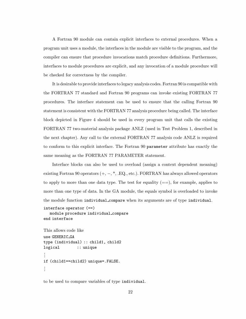
Interface blocks can also be used to overload (assign a context dependent meaning)

existing Fortran 90 operators (+, −, *, .EQ., etc.). FORTRAN has always allowed operators

to apply to more than one data type. The test for equality (==), for example, applies to

more than one type of data. In the GA module, the equals symbol is overloaded to invoke

the module function individual compare when its arguments are of type individual.

interface operator (==)

module procedure individual compare

end interface

This allows code like

use GENERIC GA

type (individual) :: child1, child2

logical :: unique...

if (child1==child2) unique=.FALSE....

to be used to compare variables of type individual.

22

interface

!

subroutine ANLZ(subpopulation size, &

individual, &

orientation array, &

material array, &

laminate size, &

fitness array, &

geometry array x, &

geometry array y)

! define parameters

! (parameters are required by

! FORTRAN 77 legacy analysis code):

integer, parameter ::

subpop maxsize=500, &

laminate maxsize=200

! define interface argument requirements:

integer :: &

orientation array(subpop maxsize, &

laminate maxsize), &

material array(subpop maxsize, &

laminate maxsize), &

subpopulation size, &

individual, &

laminate size

double precision :: &

fitness array(subpop maxsize) &

geometry array x(subpop maxsize), &

geometry array y(subpop maxsize)

end subroutine ANLZ

!

end interface

Figure 4—Fortran 90 Interface block to Test Problem 1

Whereas the interface block provides explicit type checking for procedure arguments, the

intended use of arguments is specified with the intent keyword: an argument of intent(in)

cannot be defined or redefined in the subprogram, and an argument of intent(out) must

be defined before it is referenced. The following declarations illustrate the use of intent in

the GA package procedure laminate crossover :

23

subroutine laminate crossover (parent1, &

parent2, child1, child2)

use GENERIC GA

!Declare argument intents:

type (individual), intent(in) :: &

parent1, parent2

type (individual), intent(out) :: &

child1, child2...

end subroutine laminate crossover

The parent individuals can not be modified, because they are of intent(in), and the child

individuals must be defined in the subroutine, because they are of intent(out).

With Fortran 90’s interface blocks, rigorous checking of subprogram argument types

is enabled, and with the specification of intent, user programs are forced to comply with

the intended use of subprogram arguments. Thus, while the Fortran 90 standard provides

the flexibility of modules, abstract data types, pointers, dynamic memory allocation, and

powerful array functions, the subprogram interface blocks and intent checking ensure that

procedures are invoked correctly and that variables are used as they were intended. All these

features are brought to bear in the module GENERIC GA, the GA operators package, and

the two-material test program to yield a safe, flexible, and portable framework for use in

the design optimization of composite laminate structures.

24

6. FORTRAN 90 LANGUAGE PERFORMANCE.

Test runs using Test Problem 1 (described in chapter 7) were conducted to compare the

performance of the test program with the performance of the original FORTRAN 77 code.

This test yielded optimum designs identical to those found by the original implementation.

These runs used an elitist selection scheme and operator probabilities of crossover = 1.00,

material mutation = 0.05, orientation mutation = 0.05, ply addition = 0.05, ply deletion

= 0.10, and permutation = 0.25. However, program run times are slower for the Fortran 90

implementation: for the two-material problem, the Fortran 90 version ran 1250 generations

of 25 individuals in 4 min. 23 sec., vs. 2 min. 55 sec. for the FORTRAN 77 version. This

anomaly is attributable to two factors.

First, additional time overhead is introduced in the Fortran 90 implementation by the

use of array sections. The high-level array operations described in this paper engender facile

programming and easy to understand code, but there is a run time cost associated with

copying arrays and locating the array section elements in memory. This cost is not incurred

in FORTRAN 77 codes, because accessing sections of arrays is effected directly through

low-level user-written code (DO loops). To demonstrate this, a Fortran 90 program was

written in which all the elements in each row of a large array were shifted 5 positions.

Ten repetitions of this operation took 9.1 sec. using Fortran 90 array sections, whereas

hard-coded FORTRAN 77 DO loops required only 4.6 sec. to complete the same task. The

array assignments using DO loops operate more efficiently than the equivalent array sections

Second, abstract data types make code more understandable and easy to use, but

sometimes at the expense of efficiency. For example, the hierarchy depicted in Figure 1

could be represented by a set of five dimensional arrays rather than by an abstract data

type, but the usefulness, convenience, and understandability of the population type and the

close association of this type with the GENERIC GA module would be diminished by using

the more efficient arrays. Conversely, using data types requires dereferencing of the data

type elements (or fields) in order to access the desired information. For example, accessing a

gene in individual ind in subpopulation subpop of a population using GENERIC GA data

types is achieved with a reference to the population data structure like

25

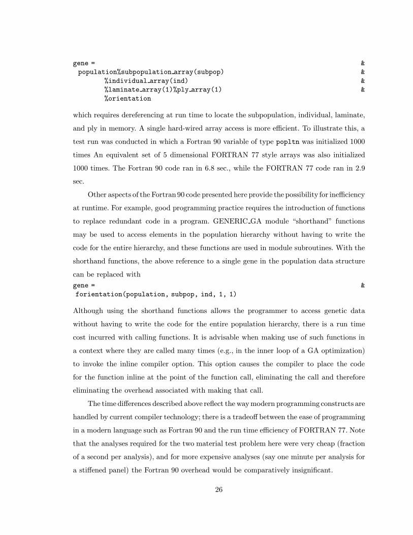
gene = &

population%subpopulation array(subpop) &

%individual array(ind) &

%laminate array(1)%ply array(1) &

%orientation

which requires dereferencing at run time to locate the subpopulation, individual, laminate,

and ply in memory. A single hard-wired array access is more efficient. To illustrate this, a

test run was conducted in which a Fortran 90 variable of type popltn was initialized 1000

times An equivalent set of 5 dimensional FORTRAN 77 style arrays was also initialized

1000 times. The Fortran 90 code ran in 6.8 sec., while the FORTRAN 77 code ran in 2.9

sec.

Other aspects of the Fortran 90 code presented here provide the possibility for inefficiency

at runtime. For example, good programming practice requires the introduction of functions

to replace redundant code in a program. GENERIC GA module “shorthand” functions

may be used to access elements in the population hierarchy without having to write the

code for the entire hierarchy, and these functions are used in module subroutines. With the

shorthand functions, the above reference to a single gene in the population data structure

can be replaced with

gene = &

forientation(population, subpop, ind, 1, 1)

Although using the shorthand functions allows the programmer to access genetic data

without having to write the code for the entire population hierarchy, there is a run time

cost incurred with calling functions. It is advisable when making use of such functions in

a context where they are called many times (e.g., in the inner loop of a GA optimization)

to invoke the inline compiler option. This option causes the compiler to place the code

for the function inline at the point of the function call, eliminating the call and therefore

eliminating the overhead associated with making that call.

The time differences described above reflect the way modern programming constructs are

handled by current compiler technology; there is a tradeoff between the ease of programming

in a modern language such as Fortran 90 and the run time efficiency of FORTRAN 77. Note

that the analyses required for the two material test problem here were very cheap (fraction

of a second per analysis), and for more expensive analyses (say one minute per analysis for

a stiffened panel) the Fortran 90 overhead would be comparatively insignificant.

26

7. TEST PROBLEMS.

Two main programs were developed to interface existing analysis codes to the GA

module and package of operators. The analyses chosen for the test programs were previously

existing FORTRAN 77 analysis packages. These optimization problems were solved with

custom-designed FORTRAN 77 GA codes, and the extensive results establish a good basis

for verifying the performance of the Fortran 90 GA module and operators package. This

chapter describes the performance criteria by which the GA analyses are evaluated. Then

the two test problems are described. Finally, the results of the test runs are presented.

The performance results of this chapter establish a baseline with which to compare the

performance of the migration algorithm presented in the next chapter.

7.1 GA Performance Analysis.

This chapter introduces the two criteria used for characterizing the performance of the

GA during a set of optimization runs: the apparent reliability and the normalized cost per

genetic search [16]. The apparent reliability R is a reflection of the reliability of the GA in

finding an optimum for a given set of conditions. R is determined by dividing the number

of runs in which at least one optimum is found by the total number of runs conducted, Nr .

The normalized cost per genetic search Cn is a reflection of the average number of

analyses required to find each unique optimum. Cn is defined by

Cn =NgP

A,

where Ng is the average number of generations per run over Nr runs, P is the size of a

subpopulation, and A is the average number of optima found per run. A is determined by

A =

Nr∑j=1

N jo

Nr,

where N jo is the number of optima found in the jth run. Ideally (R=1.0), A = 1 for problems

containing a single optimum (e.g., the first test problem) and A > 1 for problems containing

multiple optima (e.g., the second test problem).

27

7.2 Test Problem 1 Description: A Single Optimum Design Problem.

The analysis code selected for Test Problem 1 analyzes a composite laminate panel

measuring 36.0 in. by 30.0 in. The panel is simply supported an all four sides, and can

be loaded under any combination of axial and shear loads (Nx, Ny, Nxy), as depicted in

Figure 5. For simplicity, the panel is assumed to be symmetric about its midplane. This

assumption is automatically satisfied because the genetic representation of the laminate only

codes one half of the laminate. Further, the panel is required to be balanced. The balance

constraint ensures that each ply oriented at θ◦ is complemented with another ply oriented

at −θ◦ throughout the laminate stacking sequence. This constraint is enforced by means

of a penalty function in the analysis code. The analysis code determines the load handling

capability of a laminate by computing the margin of safety for its critical buckling load and

the margin of safety for its critical ply strains. The fitness value returned by the analysis

code is a measure of the panel’s weight penalized by small or violated safety margins (and

the balance constraint penalty). The goal of the GA is to minimize this fitness value. These

penalty functions are subtle, and must be chosen carefully so that an infeasible design is

not more fit than a near optimal feasible design. Such details are discussed in [17], [18].

0, +/-15, +/-30, +/-45, +/-60, +/-75, 90 deg.

36.0 in.

30.0 in.

Nx

N y

Ny

Nxy Nxy

x

z

y

midplane

Nx

plies oriented at

Figure 5—Panel configuration and loading conditions for Test Problem 1

The panel design is encoded in a single chromosome. Each gene in the chromosome

corresponds to a ply in the structure. A ply may be composed of either of two materi-

als, Graphite-epoxy (T300/N5208) and Aramid-epoxy (Kevlar 49/CE3305), so the genetic

28

alphabet for the material type genes is Vm = {1, 2}. A ply may take on any orientation

between −75◦ and 90◦, in increments of 15◦. The balance constraint in the analysis forces

plies of the same orientation and material type to take on alternating signs. For instance,

the first occurrence of the ±45◦ allele is taken to have the value +45◦, and the next oc-

currence is taken to have the value −45◦. 90◦ and 0◦ plies are not assigned a sign. Thus

the ply orientation alphabet Vo uses seven unique alleles to code the twelve ply angles,

giving Vo = {1, 2, 3, 4, 5, 6, 7} for the set of possible orientations. As an example, consider

the following chromosome strings, where each (orientation, material) pair is a gene:

orientation alleles [1 1 3 3 3 3 4 4 7 7 0 0 0 0]

material type alleles [1 1 1 1 1 2 2 2 2 2 0 0 0 0]

When this genotype is decoded by the analysis routine, the design (phenotype) is the

following:

decoded design [0(1)2 /± 30

(1)3 /± 30

(2)1 /± 45

(2)2 /90

(2)2 ]s

where θ(m)n represents n plies of material type m at orientation θ. The subscript s indicates

that the decoded design is taken to be one half the full set of plies, with the full design

symmetric about the midplane, corresponding to the right end of the string.

This particular design problem contains a single unique global optimum solution amidst

many near-optimum solutions. In order to locate this optimum (force convergence) while also

enabling the most efficient use of the GA, an elitist selection scheme is used for determining

the next generation. The elitist selection scheme works as follows. For each iteration of the

GA loop, a child population is generated. The child population is the same size as the parent

population. The elitist selection algorithm (EL) determines the most fit parent design and

retains it in the child generation, making room for the elite parent individual by discarding

the least fit child individual. Thus, the most fit design is always retained, ensuring that

each new generation’s most fit individual is at least as fit as the previous generation’s. In

addition, all but one of each new generation’s designs are unique results of the application

29

of the genetic operators, i.e., duplicate children are not permitted, ensuring diversity in the

possible solutions examined.

The input parameters to the GA module for Test Problem 1 for all GA runs in this

paper are as follows: probability of crossover pc = 1.0, probability of material mutation

pmm = 0.15, probability of orientation mutation pmo = 0.15, probability of ply addition

pa = 0.05, probability of ply deletion pd = 0.10, probability of ply swap ps = 0.75. The results

for 64 separately evolved subpopulations using the standard GA (sGA) are enumerated in

Table 1. For these runs, the subpopulation size is set to 60, and the termination criterion

for a run is 400 consecutive generations with no improvement in the best fitness.

7.3 Test Problem 2 Description: A Multiple Optimum Design Problem.

The analysis code selected for Test Problem 2 analyzes a composite laminate panel

measuring 20.0 in. by 10.0 in. The panel is simply supported an all four sides, and can be

loaded under any combination of axial loads (Nx, Ny), as depicted in Figure 6. As with

Test Problem 1, the panel is assumed to be balanced and symmetric about its midplane.

The analysis package used with this test problem determines the buckling load of a given

design by determining the critical buckling load factor. The goal of the GA is to maximize

the failure load of the laminate. In Test Problem 1, the number of plies is variable; here

the number of plies is fixed at 20.

The panel design is encoded in a single chromosome. Each gene in the chromosome

corresponds to a pair of plies in the structure. The laminate is composed of one material

(graphite epoxy) and each ply pair may take on an orientation of 0◦, ±45◦, or 90◦. Because

the plies occur in pairs, a gene coding for 0◦ decodes to two contiguous 0◦ plies, the ±45◦

gene decodes to two contiguous plies of +45◦ and −45◦ orientation, and the 90◦ gene

decodes to two contiguous 90◦ plies. The laminate is assumed to be symmetric about its

midplane, satisfying the symmetry constraint, and the balance constraint is satisfied by using

contiguous two-ply stacks. Thus, the genotype representation of the laminate represents one

fourth of the decoded phenotype.

30

0, +/-45, or 90 deg.

Nx

N y

Ny

x

z

y

midplane

Nx

plies oriented at

20.0 in.

10.0 in.

Figure 6—Panel configuration and loading conditions for Test Problem 2

The input parameters to the GA module for Test Problem 2 for all GA runs in this

paper are as follows: probability of crossover pc = 1.0, probability of material mutation

pmm = 0.0 (only one material), probability of orientation mutation pmo = 0.02, probability

of ply addition pa = 0.0, probability of ply deletion pd = 0.0, probability of ply swap

ps = 0.05, probability of ply permutation pp = 0.02. The results for 64 separately evolved

subpopulations using the standard GA (sGA) are enumerated in Table 1. For these runs,

the subpopulation size is set to 60, and the termination criterion for a run is 100 consecutive

generations with no improvement in the best fitness.

The number consecutive runs to convergence for this problem is smaller than for Test

Problem 1 (100 vs. 400), because the number of possible designs is significantly smaller for

Test Problem 2. The number of possible designs is smaller because of the smaller orientation

alphabet (three alleles here vs. seven for Test Problem 1) and the use of a single material.

The results for 64 separate optimization runs using the standard GA (sGA) are enumerated

in Table 1.

Whereas Test Problem 1 contains a single unique globally optimum solution, this

particular design problem contains a group of globally optimum designs. In order to make

efficient se of the GA, a variable elitist selection scheme is used for determining the next

generation. The multiple elitist selection algorithm is designed to retain more than one

31

individual from the parent generation in the child generation. This strategy represents a

performance tradeoff for the GA: exploitation of highly fit designs occurs by retaining elite

designs from generation to generation throughout the GA run, but exploration of further

candidate designs is compromised as the number of retained individuals is increased. Two

different multiple elitist schemes are applied to test problem 2. These strategies are inspired

by the (µ, λ) and (µ+ λ) strategies developed by Back ([21], [22]).

The first multiple elitist selection strategy (ME1) works as follows: for each iteration

of the GA loop, a child population is generated equal in size to the parent population.

The children are required to be distinct from each other and from all the parents. ME1

determines the nk most fit designs in the parent population, where nk is specified at run

time. The nk most fit parent individuals replace the nk least fit individuals of the child

generation. The nk least fit members of the child generation are discarded to make room

for the retained parents. This strategy is similar to the elitist strategy used in Test Problem

1, and, in fact, ME1 reduces to EL for nk = 1.

The second multiple elitist selection strategy (ME2) works as follows: for each iteration

of the GA loop, a child population is generated equal in size to the parent population. The

children are required to be distinct from each other and from all the parents. The parent

and child populations are combined, and the nk most fit individuals from the combined

population are determined. These nk individuals are retained in the child generation, which

is completed using the most fit remaining children, yielding a child population equal in size

to the parent population.

7.4 GA Performance Results for Test Problems 1 and 2.

For both test problems, the Fortran 90 GA implementation yielded optimum designs

identical to those found by the original custom designed FORTRAN 77 GA codes (a single

optimum for Test Problem 1, and 6 global optima for Test Problem 2). The globally optimum

designs for the two test problems are enumerated in Appendix A. Also, see [23] for a discussion

of language performance tradeoffs between the custom FORTRAN 77 codes and the Fortran

32

Table 1sGA performance results— independently evolving subpopulations.

Test Problem Selection nk Cn R A

1 EL * 65, 457 0.78 0.782 EL * 9, 182 1.0 1.002 ME1 5 2, 167 1.0 4.162 ME1 15 2, 812 1.0 3.502 ME1 30 3, 800 1.0 2.582 ME2 5 2, 320 1.0 4.152 ME2 15 2, 846 1.0 3.532 ME2 30 3, 840 1.0 2.76

* nk is not applicable for EL selection.

90 template. The test runs described in here establish a baseline for comparison with the

migration algorithm presented in the next chapter .

The normalized cost and reliability for these runs are reported in Table 1. Test Problem

1 converges with a reliability of 0.78 for EL selection. All 64 subpopulations converged (400

consecutive generations without an improvement in the best fitness), but not all converged to

the best known optimum. All 64 subpopulations did, however, converge to within 5% of the

best known optimum fitness. Generally, a reliability of 0.80–0.90 is considered acceptable,

so one of the goals of the migration algorithm is to improve R at equal or less cost.

All selection schemes for Test Problem 2 converge with a reliability of 1.0, and with

a lower normalized cost per optimum than Test Problem 1. The lower cost is attributable

to the smaller search space and the smaller genetic alphabet of Test Problem 2—there are

not as many candidate solutions to consider. A large improvement in Cn is seen when using

ME1/ME2 selection rather than EL selection. The ME selection routines exploit previously

found highly fit designs by retaining them from generation to generation. Increasing the

number of retained designs serves to increase the number of highly fit individuals involved

in the reproduction process. This is, however, at the expense of exploration. Increasing the

number of retained designs decreases the space available in the population for consideration

of new designs. This is evidenced by the increasing normalized cost of both ME schemes as

nk is increased.

In the next chapter, a distributed parallel migration algorithm is presented, and the

effect of the migration scheme on Cn and R for Test Problems 1 and 2 is explored.

33

8. PARALLEL IMPLEMENTATION.

As parallel computers become more commonplace in scientific computing, it becomes

more feasible to harness their power for use with genetic algorithms. The GA is inherently

parallel [24]. Genetic operations can be applied to individuals in a population in parallel,

a population may be partitioned into separately evolving subpopulations, or independent

runs—such as those made in Section 5—can run on different processors. A GA running in

parallel can be exploited further as an optimization tool by implementing communications

between processing elements. Indeed, Gordon and Whitley [26] report that the performance

of parallel genetic algorithms is superior to standard GAs in function optimization, even

without taking parallel hardware into account.

The migration model takes the idea of separately evolving subpopulations and extends

it by adding a means of selectively sharing genetic information between them. Migration

may occur in a variety of ways. Each processing element in a parallel GA may contain an

independently evolving standard GA which periodically migrates fit individuals to other

processors (as in [25]), or the GA itself may be parallelized. In the latter case, each individual

in a population is itself a single process, and migration is characterized as a diffusion process

as individuals reproduce within a local neighborhood (see, for example [27]).

The implementation of a distributed migration algorithm should ensure that the per-

formance of the algorithm is not constrained by the number of processors involved or by

the communication between those processors. The mechanisms of communication, load

balancing, and termination detection all determine the distributed algorithm’s parallel per-

formance. The goal of the migration algorithm presented here is to extend the sGA presented

in Section 5 to implement a migration scheme on a distributed memory parallel machine.

The present chapter describes the implementation of the distributed migration algorithm

incorporated into the Fortran 90 GA framework (the distributed GA is referred to as dGA).

All parallel code used in the dGA extension is implemented using the MPI 1.2 (Message

Passing Interface) standard for FORTRAN. Next, experiments are conducted to compare

the performance of the dGA with that of the sGA baseline established in Section 5. Section

7 quantifies the performance of the migration algorithm and the performance of the parallel

algorithm.

34

Subpop 3

Subpop 2

Subpop 1

Subpop 4

Subpop 5

Figure 7—Ring topology for migration among subpopulations

8.1 Migration.

The migration algorithm partitions a population of designs into a set of subpopulations

and, at specified intervals, shares information between these subpopulations. Tanese [29] in-

troduces the parameters associated with the migration algorithm: the migration interval

and the migration rate. The migration interval is the number of generations between each

migration, and the migration rate is the number of individuals selected for migration.

For the migration algorithm described in this paper, migrating subpopulations are

arranged in a ring topology. Migration occurs between directionally adjacent subpopulations,

as depicted in Figure 7. The migration interval is incorporated into the distributed algorithm

as a probability pm, and the migration rate is incorporated as a maximum value nm.

For each subpopulation in the distributed GA, migration is accomplished as follows. At

the end of a generation, a uniformly distributed random number y is generated. If y < pm,

migration is initiated. During migration, a uniform random number determines the number

of individuals ns between 1 and nm to send. The best ns individuals in the subpopulation

are sent to the nearest neighbor in the ring. Whether or not emigrants are sent to the

nearest neighbor, the subpopulation then checks to see if immigrants are arriving from its

neighbor. If immigrants are arriving, they are received into the subpopulation and replace

the ns least fit individuals.

35

Migration intervals are typically specified as a fixed number of generations, known

as an epoch. The problem with using a fixed epoch value is that migration is globally

synchronized across all subpopulations. Using a random interval allows the subpopulations

to evolve asynchronously. The subpopulations are not required to migrate in lockstep at a

prescribed interval. An additional advantage conferred by asynchronous migration is that

communications between the subpopulations are spread out in time more than if migration

were synchronized. This makes more efficient use of communications bandwidth and allows

quickly converging subpopulations to finish early, freeing up their processors to do more

work. Some control over average length of an epoch exists. For example, the expected value

of the epoch length for pm = 0.01 is 1/pm = 100 generations—it is expected that, on average,

migration occurs once every 100 generations for pm = 0.01.

As with multiple elitist selection, migration represents a tradeoff between exploration

of new designs and exploitation of highly fit designs which have already been found. The

physical relationship between subpopulations imposed by the topology of the distributed

system has an effect on this tradeoff as well. The ring topology used for the dGA described in

this paper ensures local communications between subpopulations. The benefit of this design

is that migration occurs locally between adjacent populations on the ring. This yields local

exploitation of fit designs, while globally the separate subpopulations are free to explore

different types of designs independently.

For composite laminate design, the analysis of individual designs is often the most

expensive part of the GA solution. Although it is reasonable to expect that larger subpop-

ulations of individuals might perform better than smaller subpopulations, increasing the

subpopulation size P results in an increase in Cn. The goal of the dGA is to achieve better

GA performance than the (serial) sGA for a given P , with a concomitant improvement in

parallel performance over a parallel sGA. Experiments designed to test the performance of

the dGA are described in Section 7.

36

8.2 An Extension to the sGA.

The standard GA is extended to yield the distributed GA with migration (dGA). Each

processing element in the dGA algorithm performs the following code:

gen = 0

initialize Population(gen)

decode and evaluate Population(gen)

while not terminated do

apply crossover to Population(gen) giving Children(gen)

apply genetic operators to Children(gen)

decode and evaluate Children(gen)

Population(gen+1) = select from(Children(gen) ∪ Population(gen+1))

!

begin migration

if migration appropriate

choose emigrants

send emigrants

end if

if immigrants available

receive immigrants

Population(gen+1) = select from(immigrants ∪ Population(gen+1))

end if

end migration

!

gen = gen + 1

check for termination

end do

8.3 Dynamic Load Balancing and Distributed Control.

Individual subpopulations in a GA run do not involve the same amount of work as other

subpopulations in the same run. Some subpopulations will converge early, and others will

converge more sluggishly, yielding a much higher normalized cost. The result is considerable

variation in the number of generations to convergence from subpopulation to subpopulation.

A simple static load balancing scheme for a parallel GA optimization using p processors and

S subpopulations might assign S/p subpopulations to each processor, and then allow each

processor to evolve those subpopulations with no further load balancing. However, due to

the variation in the number of generations to convergence, a load imbalance will inevitably

occur with this scheme, as some processors finish their work well before others finish.

37

The dGA described in this paper uses a dynamic load balancing strategy which redis-

tributes work to processors which finish their work early and become idle. The dynamic

load balancing strategy used with the dGA initially assigns S/p subpopulations to each

processor. If a processor runs out of work, it queries the other processors to see if there

is work which may be shared (greater than one remaining subpopulation on the queried

processor). This query is conducted in an asynchronous fashion, starting at the nearest

neighbor on the ring. If there is work to be shared, the two processors divide the remaining

subpopulations between themselves, and the GA algorithm is resumed. If there is no work

to be shared, the querying processor is terminated.

Sharing of work between processors is only done at the request of the receiving process,

and only the receiving process and the requested process are involved in this communication.

Thus, there is no global control of the computation; control is distributed. In order for

distributed control to be useful, a means of termination detection is required. This is

discussed next.

8.4 Termination Detection.

It is a simple enough matter to detect termination on a single processor. However,

when using multiple processors in a distributed system, termination detection becomes

more difficult because there is no knowledge of the global state of the system. The ring

topology selected for implementing the dGA is also suitable for a token passing algorithm

for detecting global termination. The token-passing algorithm used here operates as follows.

When p0 (the first processor in the ring) is finished evolving all its subpopulations, and no

other processors can share work with it, a token is passed to the next processor in the ring.

Each processor passes the token along under the same conditions. At the point when p0

receives the token again from the last processor in the ring, it is assured that all processors

in the ring have indicated a terminated state, and the global computation is thus complete.

38

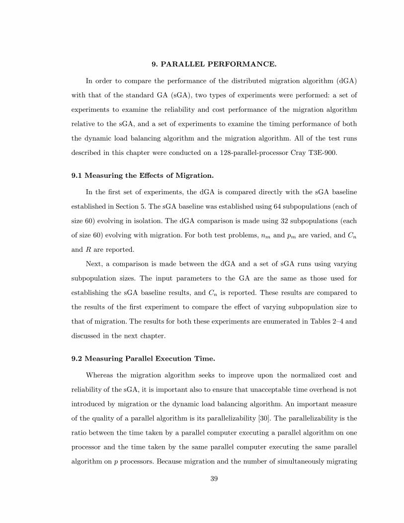
9. PARALLEL PERFORMANCE.

In order to compare the performance of the distributed migration algorithm (dGA)

with that of the standard GA (sGA), two types of experiments were performed: a set of

experiments to examine the reliability and cost performance of the migration algorithm

relative to the sGA, and a set of experiments to examine the timing performance of both

the dynamic load balancing algorithm and the migration algorithm. All of the test runs

described in this chapter were conducted on a 128-parallel-processor Cray T3E-900.

9.1 Measuring the Effects of Migration.

In the first set of experiments, the dGA is compared directly with the sGA baseline

established in Section 5. The sGA baseline was established using 64 subpopulations (each of

size 60) evolving in isolation. The dGA comparison is made using 32 subpopulations (each

of size 60) evolving with migration. For both test problems, nm and pm are varied, and Cn

and R are reported.

Next, a comparison is made between the dGA and a set of sGA runs using varying

subpopulation sizes. The input parameters to the GA are the same as those used for

establishing the sGA baseline results, and Cn is reported. These results are compared to

the results of the first experiment to compare the effect of varying subpopulation size to

that of migration. The results for both these experiments are enumerated in Tables 2–4 and

discussed in the next chapter.

9.2 Measuring Parallel Execution Time.

Whereas the migration algorithm seeks to improve upon the normalized cost and

reliability of the sGA, it is important also to ensure that unacceptable time overhead is not

introduced by migration or the dynamic load balancing algorithm. An important measure

of the quality of a parallel algorithm is its parallelizability [30]. The parallelizability is the

ratio between the time taken by a parallel computer executing a parallel algorithm on one

processor and the time taken by the same parallel computer executing the same parallel

algorithm on p processors. Because migration and the number of simultaneously migrating

39

subpopulations (the number of processing elements used in the computation) both play a role

in what Cn and R will ultimately be for a set of GA runs, it is difficult, if not impossible,

to enforce a constant amount of work across all processing elements as the number of

processing elements is varied. The parallelizability measurement, to be meaningful, relies

on the amount of (useful) work being constant as the number of processors is varied. Thus,

parallelizability is not sufficient for characterizing the performance of the dGA, because the

dGA is nondeterministic in its parallel behavior. Other performance measures are required.

The second set of experiments characterizing the dGA are intended to examine the time

effects of the migration algorithm and the dynamic load balancing algorithm. First, because

a direct measurement of parallelizability is not meaningful, an effective parallelizability

measurement is considered. For measuring the effective parallelizability, the conditions of a

GA optimization run are altered, by changing the convergence criteria for a subpopulation.

Instead of declaring convergence after a certain number of generations transpire without an

improvement in the fitness of the best individual in the subpopulation, a simple constant

number of generations is used. Each subpopulation evolves over a constant number of

generations. Next, the amount of work done in the kth subpopulation is fixed, by associating

a specific random number seed with k, independent of the number of processors used in

the run. Timing runs are made in which the number of processors is varied from 1–32, with

the total number of subpopulations (and thus the total amount of work performed) kept

constant. The effective parallelizability observed under these conditions is linear—there is

no degradation in the time performance of the dGA as the number of processors is increased.

The linear effective parallelizability under the contrived test conditions described in

the preceding paragraph is encouraging, but it is reasonable to expect that the migration

algorithm itself has a run time cost associated with it. In order to examine this assertion,

a single processor is used to conduct a GA optimization on 16 subpopulations, again using

the new, fixed convergence criteria and normalized work amount in the kth subpopulation.

The probability of migration pm is varied, and time to termination is recorded. The results

of this measurement are listed in Table 5.

40

Table 2dGA performance results, Test Problem 1 (EL selection).

nm pm Cn R(= A)

5 0.05 46,800 1.05 0.02 51,180 1.05 0.01 58,560 0.915 0.001 72,540 0.821 0.05 54,300 1.01 0.02 55,500 1.01 0.01 70,260 0.901 0.001 60,900 0.79

Table 3dGA performance results, Test Problem 2 (ME1 selection).

nm pm Cn R A5 0.05 1,670 1.0 5.225 0.02 1,844 1.0 4.535 0.01 1,980 1.0 3.975 0.001 2,175 0.96 3.471 0.05 1,540 1.0 5.161 0.02 1,721 1.0 4.721 0.01 2,032 1.0 4.311 0.001 2,194 0.94 3.38

Table 4sGA performance results for varying subpopulation size P .

Test Prob 1 (EL) Test Prob 2 (ME1)

P Cn Ng A Cn Ng A960 600,960 626 1.0 20,352 106 6.0240 172,080 717 1.0 6,840 114 4.060 65,457 1091 1.0 2,167 147 4.015 *23,190 1546 0.0 1,232 231 2.0

*optimum not found

9.3 Performance of the Migration Algorithm.

Comparing Table 1 with Tables 2 and 3, it is clear that the migration algorithm yields

an improvement in normalized cost and in reliability.

For Test Problem 1 (Table 2), an ideal reliability (R=1.0) is achieved, with a concomitant

decrease in the normalized cost per optimum found. R is 1.0 at pm = 0.05 and nm = 5, and

these values are taken to be the ideal migration parameters for Test Problem 1. As nm and

pm decrease, Cn and R both approach the values found using the sGA (Table 1).

41

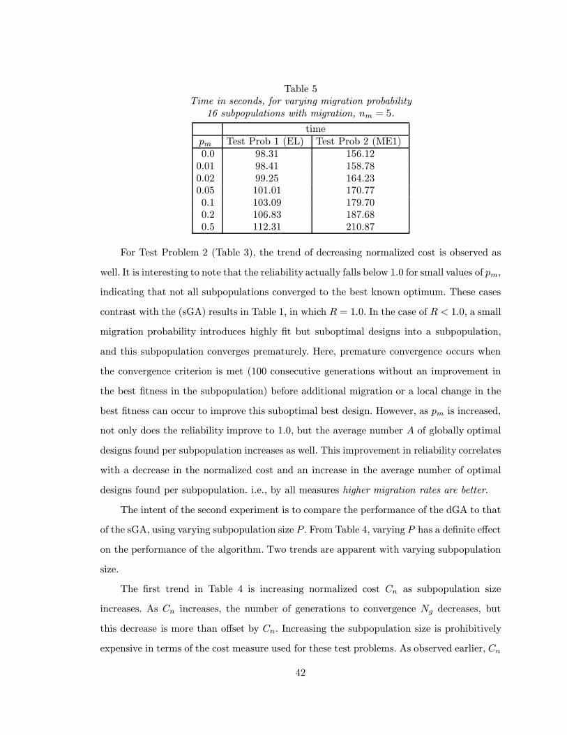
Table 5Time in seconds, for varying migration probability

16 subpopulations with migration, nm = 5.

timepm Test Prob 1 (EL) Test Prob 2 (ME1)0.0 98.31 156.12

0.01 98.41 158.780.02 99.25 164.230.05 101.01 170.770.1 103.09 179.700.2 106.83 187.680.5 112.31 210.87

For Test Problem 2 (Table 3), the trend of decreasing normalized cost is observed as

well. It is interesting to note that the reliability actually falls below 1.0 for small values of pm,

indicating that not all subpopulations converged to the best known optimum. These cases

contrast with the (sGA) results in Table 1, in which R = 1.0. In the case of R < 1.0, a small

migration probability introduces highly fit but suboptimal designs into a subpopulation,

and this subpopulation converges prematurely. Here, premature convergence occurs when

the convergence criterion is met (100 consecutive generations without an improvement in

the best fitness in the subpopulation) before additional migration or a local change in the

best fitness can occur to improve this suboptimal best design. However, as pm is increased,

not only does the reliability improve to 1.0, but the average number A of globally optimal

designs found per subpopulation increases as well. This improvement in reliability correlates

with a decrease in the normalized cost and an increase in the average number of optimal

designs found per subpopulation. i.e., by all measures higher migration rates are better.

The intent of the second experiment is to compare the performance of the dGA to that

of the sGA, using varying subpopulation size P . From Table 4, varying P has a definite effect

on the performance of the algorithm. Two trends are apparent with varying subpopulation

size.

The first trend in Table 4 is increasing normalized cost Cn as subpopulation size

increases. As Cn increases, the number of generations to convergence Ng decreases, but

this decrease is more than offset by Cn. Increasing the subpopulation size is prohibitively

expensive in terms of the cost measure used for these test problems. As observed earlier, Cn

42

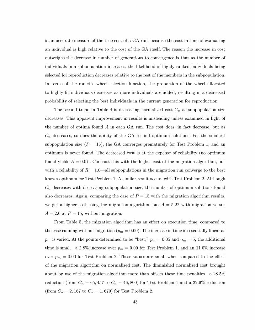
is an accurate measure of the true cost of a GA run, because the cost in time of evaluating

an individual is high relative to the cost of the GA itself. The reason the increase in cost

outweighs the decrease in number of generations to convergence is that as the number of

individuals in a subpopulation increases, the likelihood of highly ranked individuals being

selected for reproduction decreases relative to the rest of the members in the subpopulation.

In terms of the roulette wheel selection function, the proportion of the wheel allocated

to highly fit individuals decreases as more individuals are added, resulting in a decreased

probability of selecting the best individuals in the current generation for reproduction.

The second trend in Table 4 is decreasing normalized cost Cn as subpopulation size

decreases. This apparent improvement in results is misleading unless examined in light of

the number of optima found A in each GA run. The cost does, in fact decrease, but as

Cn decreases, so does the ability of the GA to find optimum solutions. For the smallest

subpopulation size (P = 15), the GA converges prematurely for Test Problem 1, and an

optimum is never found. The decreased cost is at the expense of reliability (no optimum

found yields R = 0.0) . Contrast this with the higher cost of the migration algorithm, but

with a reliability of R = 1.0—all subpopulations in the migration run converge to the best

known optimum for Test Problem 1. A similar result occurs with Test Problem 2. Although

Cn decreases with decreasing subpopulation size, the number of optimum solutions found

also decreases. Again, comparing the case of P = 15 with the migration algorithm results,

we get a higher cost using the migration algorithm, but A = 5.22 with migration versus

A = 2.0 at P = 15, without migration.

From Table 5, the migration algorithm has an effect on execution time, compared to

the case running without migration (pm = 0.00). The increase in time is essentially linear as

pm is varied. At the points determined to be “best,” pm = 0.05 and nm = 5, the additional

time is small—a 2.8% increase over pm = 0.00 for Test Problem 1, and an 11.0% increase

over pm = 0.00 for Test Problem 2. These values are small when compared to the effect

of the migration algorithm on normalized cost. The diminished normalized cost brought

about by use of the migration algorithm more than offsets these time penalties—a 28.5%

reduction (from Cn = 65, 457 to Cn = 46, 800) for Test Problem 1 and a 22.9% reduction

(from Cn = 2, 167 to Cn = 1, 670) for Test Problem 2.

43

Table 6Execution time for dynamic (td) and static (ts) load balancing, nm = 5, pm = 0.05.

S td ts *% difference

1024 2944 2983 1.3%512 1791 1822 1.7%256 920 970 5.2%128 480 516 7.0%64 247 281 12.1%32 142 153 7.1%16 96 101 4.9%8 51 51 0.0%

* (ts − td)/ts × 100%

9.4 Testing the Dynamic Load Balancing Algorithm.

In order to analyze the performance of the dynamic load balancing algorithmindependent

of the migration algorithm, migration is turned off (pm = 0.00), and the original convergence

criterion (a certain number of generations without a change in the best fitness) is turned back

on. Recall that migration, per se, has an effect on normalized cost—and thus execution time—

and this effect is dependent upon the number of processors used in the computation. Turning

off migration for analysis of the load balancing algorithm ensures that timing measurements

indicate the effects of load balancing, rather than the effects of migration. The “repeated

generations” convergence criterion is the criterion used for making the original baseline

measurements (using the sGA) in Section 5. The consequence of using this convergence

criterion is that there is much variation in the number of generations to convergence from

subpopulation to subpopulation. The dynamic load balancing algorithm compensates for

this variation by reassigning subpopulations on busy processors to idle processors. To observe

the effect on execution time of this algorithm, the number of subpopulations S is varied on

a fixed number of processors p = 8, for Test Problem 2 with ME1 selection and the same

parameters given in Section 5. For each run in this experiment, execution times for both the

dynamic load balancing algorithm td and a static load balancing algorithm ts are recorded

and enumerated in Table 6.

44

9.5 Dynamic Load Balancing Results.

From Table 6, the dynamic load balancing algorithm has some effect on diminishing

the execution time for a set of S subpopulations on p = 8 processors. At S = p the

execution times are identical for both the static and dynamic algorithms, because when a

processor runs out of work, there is no work left to be shared by the other processors in

the computation—each other processor is either completing its single subpopulation or is

finished. As S increases, the number of subpopulations originally allocated to each processor

S/p also increases. For small values of S/p > 1, the likelihood increases that there will be

some sharing of work. The amount of work shared depends on the amount of variation in the

number of generations to convergence, which in turn depends on the type of optimization

problem being solved. For the test problems addressed in this paper, the ratio between the

largest and smallest number of generations to convergence is approximately 3.0. For some

problems, this ratio can be as high as 10.0. The amount of load balancing that will be

required will vary with this ratio. At the same time, as S/p increases more, the size of the

load imbalance decreases, because the average number of generations to convergence for each

processor approaches the average on the other processors. Thus, for this algorithm there

are two factors contributing to the extent to which load balancing will affect the execution

speed of the computation: the factor S/p, and the amount of variation in the total number

of generations to convergence. Regardless of these parameters, the least improvement is at

S = p—where dynamic load balancing is only as good as static load balancing—and at high

values of S/p, where variations in the number of generations to convergence for individual

subpopulations are offset by the sheer number of subpopulations.

45

10. CONCLUSIONS.

The distributed genetic algorithm with migration (dGA) has been applied to two types

of composite laminate design problems, and its performance compared to that of the standard

GA (sGA). The migration algorithm itself results in diminished normalized cost Cn per

optima found and improved reliability R, for both of the test problems examined here.

Nondeterministic algorithms coupled with dynamic load balancing and distributed control

result in variable parallel workloads, making parallel performance evaluation complicated.

The experiments designed to characterize the parallel performance of the dynamic load

balancing algorithm with distributed control and termination detection demonstrate linear

effective parallelizability for constant workload. Finally, use of the migration algorithm

incurs a small time penalty, which is outweighed by the diminished normalized cost.

46

11. FUTURE WORK.

Positive results have been achieved using the ring communication topology. Future

work with the dGA might include an exploration of the effect of different communication

topologies, and the application of both sGA and dGA packages to other types of composite

laminate design problems. Such a study might also include a deeper exploration of the

tradeoffs associated with using higher migration rates, such as diminished diversity and

increased execution time.

47

REFERENCES.

[1] J. M. Bremermann, Optimization through evolution and recombination, Self-OrganizingSystems 7 (1958), 282–287.

[2] R. M. Friedberg, A learning machine: Part I, IBM J. of Research and Development 1(1958), 2–13.

[3] R. M. Friedberg, A learning machine: Part II, IBM J. of Research and Development 7(1959), 282–287.

[4] T. Back, Evolutionary Algorithms in Theory and Practice , Oxford University Press,NY, 1996.

[5] J. H. Holland, Adaptation in Natural and Artificial Systems, The University of MichiganPress, Ann Arbor, MI, 1976.

[6] D. E. Goldberg, Genetic Algorithms in Search, Optimization, and Machine Learning ,Addison-Wesley, Reading, MA, 1989.

[7] K. A. De Jong, An analysis of the behavior of a class of genetic adaptive systems, PhD.Dissertation, Univ. of Michigan, Ann Arbor, MI, 1975.

[8] R. T. Haftka, Elements of Structural Optimization, Kluwer Academic Publishers, Boston,1992.

[9] R. Foye, Advanced Design for Advanced Composite Airframes, Air Force MaterialsLaboratory, Wright-Patterson Air Force Base, Ohio, AFML-TR-69-251 (1969).

[10] M. E. Waddoups, Structural Airframe Application of Advanced Composite Materials—Analytical Methods, Air Force Materials Laboratory, Wright-Patterson Air Force Base,Ohio, AFML-TR-69-101 (1969).

[11] Z. Gurdal and R. T. Haftka, Optimization of Composite Laminates, Presented at theNATO Advanced Study Institute on Optimization of Large Structural Systems (1991),Berchtesgaden, Germany.

[12] R. Le Riche and R. T. Haftka, Optimization of Laminate Stacking Sequence for BucklingLoad Maximization by Genetic Algorithm, AIAA Journal 31 (1993), 951–956.

[13] R. Le Riche and R. T. Haftka, Improved Genetic Algorithm for Minimum Thick-ness Composite Laminate Design, Proceedings of International Conf. on CompositeEngineering, (1994), New Orleans, LA.

[14] N. Kogiso, L. T. Watson, Z. Gurdal, R. T. Haftka, and S. Nagendra, Design of CompositeLaminates by a Genetic Algorithm with Memory, Mechanics of Composite Materialsand Structures 1 (1994), 95–117.

[15] N. Kogiso, L. T. Watson, Z. Gurdal, and R. T. Haftka, Genetic algorithms with localimprovement for composite laminate design, Structural Optim. 7 (1994), 207–218.

[16] G. A. Soremekun, Genetic Algorithms for Composite Laminate Design and Optimization,MS Thesis, Department of Engineering Mechanics, Virginia Polytechnic Institute andState University, Blacksburg, VA, 1997.

[17] S. Nagendra, D. Jestin, Z. Gurdal, R. T. Haftka, and L. T. Watson, Improved geneticalgorithms for the design of stiffened composite panels, Comput. & Structures 58 (1996),543–555.

[18] S. Nagendra, S., Z. Gurdal, R. T. Haftka, and L. T. Watson, “Derivative based approx-imation for predicting the effect of changes in laminate stacking sequence”, StructuralOptim. 11 (1996), 235–243.

48

[19] S. Nagendra, R. T. Haftka, and Z. Gurdal, Design of Blade Stiffened Composite Panelsby a Genetic Algorithm Approach, Proceedings of the 34th AIAA/ASME/AHS SDMConf., La Jolla, CA, (1993), 2418–2436.

[20] S. Nagendra, R. T. Haftka, and Z. Gurdal, PASCO-GA : A Genetic Algorithm basedDesign Procedure For Stiffened Composite Panels under Stability and Strain Constraints,TenthDOD/NASA/FAA Conf. on Fibrous Composites in Structural Design, Hilton Head,SC, (1993).

[21] T. Back and F. Hoffmeister, Extended Selection Mechanisms in Genetic Algorithms, Pro-ceedings of the 4th International Conference on Genetic Algorithms, Morgan KaufmannPublishers, San Mateo, CA, (1991), 92–99.

[22] T. Back, Selective Pressure in Evolutionary Algorithms: A Characterization of SelectionMechanisms, Proceedings of the First International IEEE Conference on EvolutionaryComputation, IEEE Press, NY, (1994), 57–62.

[23] M. T. McMahon, L. T. Watson, G. A. Soremekun, Z. Gurdal, and R. T. Haftka,A Fortran 90 Genetic Algorithm Module for Composite Laminate Structure Design,Engineering with Computers (1998).

[24] J. J. Grefenstette and J. E. Baker, How genetic algorithmswork: A critical look at implicitparallelism, Proceedings of the Third International Conference on Genetic Algorithmsand Their Applications, Morgan Kaufmann, San Mateo, CA, (1989), 20–27.

[25] J. P. Cohoon, S. U. Hedge, W. N. Martin, and D. Richards, Punctuated equilibria: Aparallel genetic algorithm, Proceedings of the Third International Conference on GeneticAlgorithms and Their Applications, Morgan Kaufmann, San Mateo, CA, (1987), 750–755.

[26] V. S. Gordon and D. Whitley, Serial and Parallel Genetic Algorithms as FunctionOptimizers, Proceedings of the Fifth International Conference on Genetic Algorithmsand Their Applications, Morgan Kaufmann, San Mateo, CA, (1993), 177–183.

[27] M. Gorges-Schleuter, Asparagos: an asynchronous parallel genetic optimization strategy,Proceedings of the Third International Conference on Genetic Algorithms and TheirApplications, Morgan Kaufmann, San Mateo, CA, (1987), 422–427.

[28] F. Hoffmeister, Scalable Parallelism by Evolutionary Algorithms, Lecture Notes inEconomics and Mathematical Systems 367 (1991), Springer Verlag, Berlin, 177–198.

[29] R. Tanese, Distributed Genetic Algorithms, Proceedings of the Third InternationalConference on Genetic Algorithms and Their Applications, Morgan Kaufmann, SanMateo, CA, (1989), 434–439.

[30] M. J. Quinn, Parallel Computing, Theory and Practice, McGraw-Hill, NY, 1994.

49

Appendix A: Optimum designs for Test Problems 1 & 2.

The single globally optimum design for Test Problem 1.

Design Rank Stacking Sequence Weight Fitness

1 ±45(2)6 /90

(1)1 /± 45

(1)4 0.757259 −0.757158

The six globally optimum designs for Test Problem 2

Design Rank Stacking Sequence Buckling Factor Fitness

1 90◦4/± 45◦4/90◦8 3973.01 3973.01

2 ±45◦2/90◦10/± 45◦2/90◦2 3973.01 3973.01

3 ±45◦2/90◦8/± 45◦2/90◦4 3973.01 3973.01

4 90◦6/± 45◦2/90◦2/± 45◦2/90◦2/± 45◦2 3973.01 3973.01

5 90◦2/± 45◦2/90◦4/± 45◦2/0◦2/90◦2/± 45◦2 3973.01 3973.01

6 90◦2/± 45◦2/90◦8/± 45◦1/90◦2 3973.01 3973.01

50

Appendix B: Fortran 90 Code.

The Fortran 90 GA module, package of operators, and selection schemed described in

Chapters 3, 4, and 5 are listed here.

B.1 The Genetic Algorithm Module.

C---------------------------------------------------------------------

module GENERIC_GA

!======================================================================

!The module GENERIC_GA provides data structures for use in designing

!composite materials with genetic algorithms.

!Data structures are supplied for all entities found in a population of

!composite structures.

!

!A population is a structure defined in this module.

!Variables of type (POPLTN) inherit this structure and can be initialized

!and manipulated by module functions and subprograms. Schematically,

!the population structure is:

!

! Population

! |

! Subpopulations

! |

! Individuals

! | |

! Laminate Chromosomes Geometry Chromosomes

! | |

! Ply Genes Geometry Genes

! | |

! |orientation |digit

! |material

!

!

!The individual attributes for a population in this module are stored

!in a structure, inherited by using type (INDIVIDUAL_ATTRIBS). The

!module global variable INDIVIDUAL_ATTRIBUTES of type (INDIVIDUAL_ATTRIBS)

!is used to define all attributes of an individual. INDIVIDUAL_ATTRIBUTES

!serves as a means of communicating user-defined data (e.g., from an

!input file) to the module. Schematically, the INDIVIDUAL_ATTRIBUTES

!structure is:

!

! Individual Attributes

! | |

! |size_lam |size_geom

! | |

! Laminate Attributes Geometry Attributes

! | |

! |laminate chromo size |geometry chromo size

! |crossover type |upper bounds array

! |mutation type |lower bounds array

! |empty plies |

! | |prob_mutation

! |num materials |prob_crossover

! |material array

51

! |

! |num orientations

! |orientation array

! |

! |prob_crossover

! |prob_mut_orientation

! |prob_mut_material

! |prob_ply_addition

! |prob_ply_deletion

! |prob_intra_ply_swap

! |prob_permutation

!

!Variables used in defining a population:

!

! POPULATION_SIZE specifies the number of subpopulations in a population.

! SUBPOPULATION_SIZE specifies the number of individuals in a subpopulation.

!

!Functions contained in this module:

!

! FINDIVIDUAL

! FORIENTATION

! FMATERIAL

! FSTRUCTURE

! FGEOMETRY

! FINDIVIDUAL_COMPARE

! CREATE_CHILD

!

!Subroutines contained in this module:

!

! INITIALIZE_POPULATION

! RANDOMIZER

!

!===========================================================================

!!!!!!!!!!!!!!!!!!!!!!!!!!!!!!

! genetic data types

!!!!!!!!!!!!!!!!!!!!!!!!!!!!!!

! Create specifications for numbers.

! 2-digit integers

integer, parameter :: small = selected_int_kind(2)

! 64-bit IEEE reals

integer, parameter :: R8 = selected_real_kind(15,307)

! Population variables:

integer :: population_size, subpopulation_size

!!!!!!!!!!!!!!!!!!!!!!!!!!!!!!!!!!!!!!!!!!!!!!!!!!!!!!!!!!!!!!!!!!!!!!!!!!!!!!!

! Gene data types:

type ply_gene

integer (KIND=small) ::orientation

integer (KIND=small) ::material

end type ply_gene

type geometry_gene

real (KIND=R8) ::digit

end type geometry_gene

! Chromosome data types:

type laminate_chromosome

type (ply_gene), pointer, dimension(:):: ply_array

end type laminate_chromosome

52

type geometry_chromosome

type (geometry_gene), pointer, dimension(:):: &

geometry_gene_array

end type geometry_chromosome

! Individual (structure) data type:

type individual

type (laminate_chromosome),pointer,dimension(:):: &

laminate_array

type (geometry_chromosome),pointer,dimension(:):: &

geometry_array

end type individual

! Subpopulation data type:

type subpopulation

type (individual), pointer, dimension(:):: &

individual_array

end type subpopulation

! Population data type:

type popltn

type (subpopulation), pointer, dimension(:):: &

subpopulation_array

end type popltn

!!!!!!!!!!!!!!!!!!!!!!!!!!!!!!!!!!!!!!!!!!!!!!!!!!!!!!!!!!!!!!!!!!!!!!!!!!!!!!!!

! Data types for individual attributes:

! Types for each laminate’s attribute definitions

type laminate_attributes

integer :: laminate_size

integer :: crossover_type

integer :: mutation_type

logical :: empty_plies

integer :: num_materials

integer, pointer, dimension(:) :: material_array

integer :: num_poss_orientations

integer, pointer, dimension(:) :: orientation_array

real (KIND = R8) :: prob_crossover, prob_mut_orientation, &

prob_mut_material, &

prob_ply_addition, prob_ply_deletion, &

prob_intra_ply_swap, prob_permutation

end type laminate_attributes

! Types for each geometry’s attribute definitions:

type geometry_attributes

integer :: geom_chromo_size

real (KIND = R8), pointer, dimension(:) :: lower_bounds_array

real (KIND = R8), pointer, dimension(:) :: upper_bounds_array

real (KIND = R8) :: prob_mutation, prob_crossover

end type geometry_attributes

! Type for individual attributes:

type individual_attribs

integer :: individual_size_lam

integer :: individual_size_geom

real (KIND = R8) :: prob_inter_ply_swap

type (laminate_attributes), pointer, dimension(:):: &

laminate_definition_array

type (geometry_attributes),pointer, dimension(:):: &

geometry_definition_array

end type individual_attribs

!!!!!!!!!!!!!!!!!!!!!!!!!!!!!!!!!!!!!!!!!!!!!!!!!!!!!!

53

!Global variables:

! The variable INDIVIDUAL_ATTRIBUTES is used to specify an

! individual.

! It must be initialized by the user before this module is useable.

type (individual_attribs) :: individual_attributes

type (individual) :: empty_individual

!!!!!!!!!!!!!!!!!!!!!!!!!!!!!!!!!!!!!!!!!!!!!!!!!!!!!!!!!!!!!!!!!!!!!!!!!!!!!!!!

!Interface definition:

!The following interface allows the comparison of individuals by means of a

!check for equality (’==’ or ’.eq’).

interface operator (.eq.)

module procedure findividual_compare

end interface

!!!!!!!!!!!!!!!!!!!!!!!!!!!!!!!!!!!!!!!!!!!!!!!!!!!!!!!!!!!!!!!!!!!!!!!!!!!!!!!!

contains

!!!!!!!!!!!!!!!!!!!!!!!!!!!!!!!!!!!!!!!!!!!!!!!!!!!!!!!!!!!!!!!!!!!!!!!!!!!!!!!

! The following are shorthand functions for accessing genetic data.

! The shorthand functions provide a means of accessing data without the need

! to reference through the hierarchy of data types

!

! For example,

! value = forientation(pop, 1, 2, 3, 4)

! is tantamount to

! value = population%subpopulation_array(1)%individual_array(2)% &

! laminate_array(3)%ply_array(4)%orientation .

!

!!!!!!!!!!!!!!!!!!!!!!!!!!!!!!!!!!!!!!!!!!!!!!!!!!!!!!!!!!!!!!!!!!!!!!!!!!!!!!!

function FINDIVIDUAL (POPULATION, J, K) result (VALUE)

!

!Function findividual returns the specified individual from the population.

!

! On input:

!

! POPULARTION specifies the population the individual is in.

!

! J specifies the subpopulation number in the population.

!

! K specifies the individual number in the subpopulation.

!

! On output:

!

! VALUE is the specified individual, of type (individual).

!

!!!!!!!!!!!!!!!!!!!!!!!!!!!!!!!!!!!!!!!!!!!!!!!!!!!!!!!!!!!!!!!!!!!!!!!!!!!!!!!

type (popltn) :: population

type (individual) :: value

integer ::j, k

value = population%subpopulation_array(j)%individual_array(k)

return

end function FINDIVIDUAL

!!!!!!!!!!!!!!!!!!!!!!!!!!!!!!!!!!!!!!!!!!!!!!!!!!!!!!!!!!!!!!!!!!!!!!!!!!!!!!!!

!!!!!!!!!!!!!!!!!!!!!!!!!!!!!!!!!!!!!!!!!!!!!!!!!!!!!!!!!!!!!!!!!!!!!!!!!!!!!!!!

function FORIENTATION (POPULATION, J, K, M, N) result (VALUE)

!

! Function FORIENTATION returns the orientation value for the specified

! individual.

54

!

! On input:

!

! POPULATION specifies the population the individual is in. population is of

! type (population), defined in this module.

!

! J specifies the subpopulation number in the population.

!

! K specifies the individual number in the subpopulation.

!

! M specifies the the laminate number in the individual.

!

! N specifies the ply number in the laminate.

!

! On output:

!

! VALUE is the specified orientation, of type integer.

!

!!!!!!!!!!!!!!!!!!!!!!!!!!!!!!!!!!!!!!!!!!!!!!!!!!!!!!!!!!!!!!!!!!!!!!!!!!!!!!!!

type (popltn) :: population

integer :: j, k, m, n

integer (KIND=small) :: value

value = population%subpopulation_array(j)%individual_array(k)% &

laminate_array(m)%ply_array(n)%orientation

return

end function FORIENTATION

!!!!!!!!!!!!!!!!!!!!!!!!!!!!!!!!!!!!!!!!!!!!!!!!!!!!!!!!!!!!!!!!!!!!!!!!!!!!!!!

!!!!!!!!!!!!!!!!!!!!!!!!!!!!!!!!!!!!!!!!!!!!!!!!!!!!!!!!!!!!!!!!!!!!!!!!!!!!!!!!

function FMATERIAL(POPULATION, J, K, M, N) result (VALUE)

!

! Function FMATERIAL returns the material value for the specified individual.

!

! On input:

!

! POPULATION specifies the population the individual is in.

!

! J specifies the subpopulation number in the population.

!

! K specifies the individual number in the subpopulation.

!

! M specifies the the laminate number in the individual.

!

! N specifies the ply number in the laminate.

!

! On output:

!

! VALUE is the specified material, of type integer.

!

!!!!!!!!!!!!!!!!!!!!!!!!!!!!!!!!!!!!!!!!!!!!!!!!!!!!!!!!!!!!!!!!!!!!!!!!!!!!!!!!

type (popltn) :: population

integer :: j, k, m, n

integer (KIND=small) :: value

value = population%subpopulation_array(j)%individual_array(k)% &

laminate_array(m)%ply_array(n)%material

return

end function FMATERIAL

55

!!!!!!!!!!!!!!!!!!!!!!!!!!!!!!!!!!!!!!!!!!!!!!!!!!!!!!!!!!!!!!!!!!!!!!!!!!!!!!!

!!!!!!!!!!!!!!!!!!!!!!!!!!!!!!!!!!!!!!!!!!!!!!!!!!!!!!!!!!!!!!!!!!!!!!!!!!!!!!!!

function FGEOMETRY(POPULATION, J, K, M, N) result (VALUE)

!

! Function FGEOMETRY returns the geometry value for the specified individual.

!

! On input:

!

! POPULATION specifies the population the individual is in.

!

! J specifies the subpopulation number in the population.

!

! K specifies the individual number in the subpopulation.

!

! M specifies the the geometry chromosome number in the individual.

!

! N specifies the geometry gene number in the laminate.

!

! On output:

!

! VALUE is the specified geometry value, of type real.

!

!!!!!!!!!!!!!!!!!!!!!!!!!!!!!!!!!!!!!!!!!!!!!!!!!!!!!!!!!!!!!!!!!!!!!!!!!!!!!!!!

type (popltn) :: population

integer :: j, k, m, n

real (KIND=R8) :: value

value = population%subpopulation_array(j)%individual_array(k)% &

geometry_array(m)%geometry_gene_array(n)%digit

return

end function FGEOMETRY

!!!!!!!!!!!!!!!!!!!!!!!!!!!!!!!!!!!!!!!!!!!!!!!!!!!!!!!!!!!!!!!!!!!!!!!!!!!!!!

!!!!!!!!!!!!!!!!!!!!!!!!!!!!!!!!!!!!!!!!!!!!!!!!!!!!!!!!!!!!!!!!!!!!!!!!!!!!!!

function FSTRUCTURE(POPULATION, J, K) result (VALUE)

!

! Function FSTRUCTURE returns an individual structure from the population.

!

! On input:

!

! POPULATION specifies the population the individual is in.

!

! J specifies the subpopulation number in the population.

!

! K specifies the individual number in the subpopulation.

!

! On output:

!

! VALUE is the specified individual structure, of type (individual).

!

!!!!!!!!!!!!!!!!!!!!!!!!!!!!!!!!!!!!!!!!!!!!!!!!!!!!!!!!!!!!!!!!!!!!!!!!!!!!!!!!

type (popltn) :: population

type (individual):: value

integer :: j, k

value = population%subpopulation_array(j)%individual_array(k)

return

end function FSTRUCTURE

!!!!!!!!!!!!!!!!!!!!!!!!!!!!!!!!!!!!!!!!!!!!!!!!!!!!!!!!!!!!!!!!!!!!!!!!!!!!!!!

56

!End shorthand functions.

!!!!!!!!!!!!!!!!!!!!!!!!!!!!!!!!!!!!!!!!!!!!!!!!!!!!!!!!!!!!!!!!!!!!!!!!!!!!!!

function FINDIVIDUAL_COMPARE(STRUCT1, STRUCT2) result (IND_VALUE)

!

! Function FINDIVIDUAL_COMPARE compares two individuals (structures)

! for equality.

!

! On input:

!

! STRUCT1 is the first individual to compare.

!

! STRUCT2 is the second individual to compare.

!

! On output:

!

! IND_VALUE is .TRUE. if the structures are identical, or

! is .FALSE. if the structures differ in at least one material

! or orientation.

!

! NOTE : This function is also accessed through the interface operator (.eq.),

! which enables the function to be used as a binary (infix) operator

!

! For example,

! if (child1 == child2) then ...

! and

! if (child1 .eq. child2) then ...

! are equivalent to

! if (findividual_compare(child1, child2)) then ...

!

! NOTE : This function only compares orientations and material types, not

! continuous (geometry) variables

!

!!!!!!!!!!!!!!!!!!!!!!!!!!!!!!!!!!!!!!!!!!!!!!!!!!!!!!!!!!!!!!!!!!!!!!!!!!!!!!!

!struct1 and struct2 are intent in to enable access through an interface.

type (individual), intent(in) :: struct1

type (individual), intent(in) :: struct2

logical :: ind_value

!Local variables:

integer :: L, M

ind_value = .TRUE.

Lloop:do L = 1, individual_attributes%individual_size_lam

Mloop: do M=1,individual_attributes%laminate_definition_array(L)% &

laminate_size

if (.NOT.((struct1%laminate_array(L)%ply_array(M)%orientation== &

struct2%laminate_array(L)%ply_array(M)%orientation) .and. &

(struct1%laminate_array(L)%ply_array(M)%material == &

struct2%laminate_array(L)%ply_array(M)%material))) &

then

ind_value = .FALSE.

exit Mloop

end if

end do Mloop

end do Lloop

return

end function FINDIVIDUAL_COMPARE

!!!!!!!!!!!!!!!!!!!!!!!!!!!!!!!!!!!!!!!!!!!!!!!!!!!!!!!!!!!!!!!!!!!!!!!!!!!!!!

57

!!!!!!!!!!!!!!!!!!!!!!!!!!!!!!!!!!!!!!!!!!!!!!!!!!!!!!!!!!!!!!!!!!!!!!!!!!!!!!

function CREATE_CHILD() result(CHILD)

!

!Function CREATE_CHILD creates a new structure.

!

! On input:

!

! Data necessary to define a new individual is available in the

! individual_attributes variable, defined in this module, and initialized

! in a user program

!

! On output:

!

! CHILD is a new individual, of type (individual),

! with all values initialized to zero.

!

!!!!!!!!!!!!!!!!!!!!!!!!!!!!!!!!!!!!!!!!!!!!!!!!!!!!!!!!!!!!!!!!!!!!!!!!!!!!!!

type (individual) :: child

!Local variables:

integer :: subpopulation

integer :: L, M, N, P

!allocate laminates

allocate (child%laminate_array(individual_attributes%individual_size_lam))

Lloop:do L=1, individual_attributes%individual_size_lam

allocate (child%laminate_array(L)%ply_array( &

individual_attributes%laminate_definition_array(L)% &

laminate_size))

Mloop:do M=1, individual_attributes%laminate_definition_array(L)% &

laminate_size

child%laminate_array(L)%ply_array(M)%orientation = 0

child%laminate_array(L)%ply_array(M)%material = 0

end do Mloop

end do Lloop

!allocate geometries

allocate (child%geometry_array(individual_attributes% &

individual_size_geom))

Nloop:do N=1, individual_attributes%individual_size_geom

allocate (child%geometry_array(N)%geometry_gene_array( &

individual_attributes%geometry_definition_array(N)%geom_chromo_size))

Ploop:do P=1, individual_attributes%geometry_definition_array(N)% &

geom_chromo_size

child%geometry_array(N)%geometry_gene_array(P)%digit = 0

end do Ploop

end do Nloop

return

end function CREATE_CHILD

!!!!!!!!!!!!!!!!!!!!!!!!!!!!!!!!!!!!!!!!!!!!!!!!!!!!!!!!!!!!!!!!!!!!!!!!!!!!!

!!!!!!!!!!!!!!!!!!!!!!!!!!!!!!!!!!!!!!!!!!!!!!!!!!!!!!!!!!!!!!!!!!!!!!!!!!!!!

subroutine INITIALIZE_POPULATION(POPULATION)

!

! Subroutine INITIALIZE_POPULATION creates and initializes a new population,

! with individuals created according to the variable, INDIVIDUAL_ATTRIBUTES.

!

!

!

! On input:

58

!

! Data necessary to define a population is available in the

! variables INDIVIDUAL_ATTRIBUTES, POPULATION_SIZE, and SUBPOPULATION_SIZE,

! defined in module GENERIC_GA, and initialized in a user program.

! Individual’s gene values (geometry, material, and orientation) are

! initialized randomly according to INDIVIDUAL_ATTRIBUTES.

!

!

! On output:

!

! POPULATION is the initialized population, of type (popltn).

!

!

! Other functions and subroutines used:

!

! Function CREATE_CHILD creates individuals to be added to the population.

!

! Function FINDIVIDUAL_COMPARE is used to compare individuals for uniqueness.

! This function is accessed with the "==" operator, as defined in the

! interface block of this module.

!

!!!!!!!!!!!!!!!!!!!!!!!!!!!!!!!!!!!!!!!!!!!!!!!!!!!!!!!!!!!!!!!!!!!!!!!!!!!!!

type (popltn), intent(out) :: POPULATION

!Local variables:

integer :: orientation, geom_gene_num

integer :: J,K,L,M,N,P,Q, count

real (KIND=R8) :: rnd, x1, x2, geom_digit

logical :: unique_indiv

empty_individual=create_child()

!Allocate space for populations.

allocate (population%subpopulation_array(population_size))

!Allocate space for subpopulations.

Jloop:do J=1, population_size

allocate (population%subpopulation_array(J)% &

individual_array(subpopulation_size))

!Create a subpopulation of individuals.

Kloop:do K=1, subpopulation_size

population%subpopulation_array(J)%individual_array(K)= &

create_child()

count = 0 ! Count attempts to find unique child.

unique:do !Check for uniqueness of each child w.r.t. the population.

count = count + 1

!Randomly initialize ply genes.

Lloop:do L=1, individual_attributes%individual_size_lam

Mloop:do M=1, individual_attributes%laminate_definition_array(L)% &

laminate_size

call random_number(rnd)

if (individual_attributes%laminate_definition_array(L)% &

empty_plies .eqv. .FALSE.) then

population%subpopulation_array(J)%individual_array(K)% &

laminate_array(L)%ply_array(M)%orientation &

=individual_attributes%laminate_definition_array(L)% &

orientation_array(ceiling(rnd*individual_attributes% &

laminate_definition_array(L)%num_poss_orientations))

else

if (rnd < 1.0/(individual_attributes% &

59

laminate_definition_array(L)%num_poss_orientations+1)) &

then

population%subpopulation_array(J)%individual_array(K)% &

laminate_array(L)%ply_array(M)%orientation &

= 0 ! empty ply

else

call random_number(rnd)

population%subpopulation_array(J)%individual_array(K)% &

laminate_array(L)%ply_array(M)%orientation &

=individual_attributes%laminate_definition_array(L)% &

orientation_array(ceiling(rnd*(individual_attributes% &

laminate_definition_array(L)%num_poss_orientations )) )

endif

endif

if (forientation(population, J, K, L, M) == 0) then

population%subpopulation_array(J)%individual_array(K)% &

laminate_array(L)%ply_array(M)%material=0

else

call random_number(rnd)

population%subpopulation_array(J)%individual_array(K)% &

laminate_array(L)%ply_array(M)%material &

=individual_attributes%laminate_definition_array(L)% &

material_array(ceiling(rnd*(individual_attributes% &

laminate_definition_array(L)%num_materials )) )

endif

end do Mloop

population%subpopulation_array(J)%individual_array(K)% &

laminate_array(L)%ply_array(1:) = &

pack (population%subpopulation_array(J)%individual_array(K)% &

laminate_array(L)%ply_array, mask = population%subpopulation_array(J)% &

individual_array(K)%laminate_array(L)%ply_array%orientation .ne. 0, &

vector = (empty_individual%laminate_array(L)%ply_array) )

end do Lloop

!Randomly initialize geometry genes.

Nloop:do N=1, individual_attributes%individual_size_geom

Ploop: do P=1, individual_attributes%geometry_definition_array(N)% &

geom_chromo_size

x1 = individual_attributes%geometry_definition_array(N)% &

lower_bounds_array(P)

x2 = individual_attributes%geometry_definition_array(N)% &

upper_bounds_array(P)

call random_number(rnd)

geom_digit = x1 + rnd*(x2-x1)

population%subpopulation_array(J)%individual_array(K)% &

geometry_array(N)%geometry_gene_array(P)%digit=geom_digit

end do Ploop

end do Nloop

!Check for uniqueness against population.

unique_indiv = .TRUE.

Qloop: do Q=1,K-1 ! compare to all preceeding

if ((population%subpopulation_array(J)%individual_array(K)) &

== (population%subpopulation_array(J)%individual_array(Q))) then

unique_indiv = .FALSE.

exit Qloop

end if

end do Qloop

60

if ((unique_indiv) .or. (count==200)) exit unique

end do unique

end do Kloop

end do Jloop

return

end subroutine INITIALIZE_POPULATION

!!!!!!!!!!!!!!!!!!!!!!!!!!!!!!!!!!!!!!!!!!!!!!!!!!!!!!!!!!!!!!!!!!!!!!!!!!!!!!!!

!!!!!!!!!!!!!!!!!!!!!!!!!!!!!!!!!!!!!!!!!!!!!!!!!!!!!!!!!!!!!!!!!!!!!!!!!!!!!!!!

subroutine RANDOMIZER

!

! Subroutine RANDOMIZER seeds the f90 random number generator.

!

! On Input:

!

! The seed for the random number generator is in this subprogram. No inputs

! are necessary.

!

! On output:

!

! There is no return value. The random number generator is initialized.

!

!!!!!!!!!!!!!!!!!!!!!!!!!!!!!!!!!!!!!!!!!!!!!!!!!!!!!!!!!!!!!!!!!!!!!!!!!!!!!!!!

!Local variables:

integer, allocatable, dimension(:) :: seed

integer :: seed_size

call random_seed (SIZE=seed_size)

allocate (seed(seed_size))

seed=2345

call random_seed (PUT=seed(1:seed_size))

return

end subroutine RANDOMIZER

!!!!!!!!!!!!!!!!!!!!!!!!!!!!!!!!!!!!!!!!!!!!!!!!!!!!!!!!!!!!!!!!!!!!!!!!!!!!!!!!

end module GENERIC_GA

61

B.2 The Genetic Algorithm Package of Operators.

subroutine APPLY_OPERATORS(POPULATION, PARENT_RANK_ARRAY, CHILD_POPULATION, &

INTERVAL_ARRAY)

!

! Subroutine APPLY_OPERATORS applies the genetic operators in

! this package to a population, and returns a child population.

!

! The subroutine employs a loop, which iterates until the child

! population is full of unique individuals.

! Within the loop, two parents are selected at

! random, using PARENT_RANK_ARRAY and INTERVAL_ARRAY; crossover

! is applied to these parents, yielding two new children; then,

! the MUTATION, ADDITION, DELETION, INTRA_PLY_SWAP, and

! PERMUTATION operators are applied to each of these children.

! A child is added to the child subpopulation if it is unique

! w.r.t the parent subpopulation and the other children in the

! child subpopulation.

!

!

! On input:

!

! POPULATION is the parent population from which the new child

! population is created.

!

! PARENT_RANK_ARRAY is an array holding the rank of each

! individual in each parent subpopulation. It is expected that

! the nth rank array entry for any subpopulation will give the

! position in the subpopulation of the individual of rank n.

! There is a unique rank for each member of a subpopulation.

!

! For example,

! If PARENT_RANK_ARRAY(3,1) is equal to 7, then the seventh

! individual in the parent subpopulation (subpopulation 3 in

! this example) has the highest rank (best fitness).

!

!

! INTERVAL_ARRAY is an array of intervals used to randomly

! choose parents from a subpopulation. The real values in this

! array specify intervals corresponding to the desired

! probability that a given ranked parent will be chosen.

!

! For example,

! If a subpopulation has size 3, and the entries in the

! interval array are (x,y,z), then if uniform random variable q

! has a value less than or equal to x, the first individual in the

! parent subpopulation is chosen. If q has a value in the interval

! (x,y], then the second individual in the parent

! subpopulation is chosen, and if q has a value in the interval

! (y,z], the third individual in the parent subpopulation is

! chosen.

!

!

! On output:

!

! CHILD_POPULATION contains a unique set of children resulting

62

! from applying the genetic operators in this package.

!

!

! Other functions (f) and subroutines (s) called in this

! subroutine:

!

! 1) CREATE_CHILD (f)

! 2) CROSSOVER (s)

! 3) MUTATION (s)

! 4) ADDITION (s)

! 5) DELETION (s)

! 6) PERMUTATION (s)

! 7) INTRA_PLY_SWAP (s)

!

!

!!!!!!!!!!!!!!!!!!!!!!!!!!!!!!!!!!!!!!!!!!!!!!!!!!!!!!!!!!!!!!!!

use GENERIC_GA

type (popltn), intent(in) :: population

type (popltn), intent(inout) :: child_population

real (KIND=R8), intent(in) :: interval_array(subpopulation_size)

integer, intent(in) :: parent_rank_array(population_size, &

subpopulation_size)

!Local variables

type (individual) :: child_1, child_2, parent_1, parent_2, last_reject

integer :: subpop,i,j,m,q, child_subpop_size, &

index1, index2

integer :: iteration_count, counter

logical :: unique, unique1, unique2

real (KIND = R8) :: rnd

popLoop: do subpop = 1,population_size

child_subpop_size = 0

iteration_count = 0

unique1 = .TRUE.

unique2 = .TRUE.

child_1 = child_population%subpopulation_array(subpop)% &

individual_array(1)

child_2 = child_population%subpopulation_array(subpop)% &

individual_array(2)

uniqueloop: do !Iterate through until child population is full.

iteration_count = iteration_count+1

!Select parents.

select: do ! Until different parents have been chosen.

call random_number(rnd)

Iloop: do I = 1, subpopulation_size

if (rnd <= interval_array(I)) then

index1 = parent_rank_array(subpop, I)

exit

end if

end do Iloop

call random_number(rnd)

do I = 1, subpopulation_size

if (rnd <= interval_array(I)) then

index2 = parent_rank_array(subpop, I)

exit

end if

end do

63

if (index1 /= index2) exit

end do select

parent_2 = population%subpopulation_array(subpop)%individual_array(index2)

parent_1 = population%subpopulation_array(subpop)%individual_array(index1)

!Select parent section is complete.

call crossover(parent_1, parent_2,child_1,child_2)

call mutation(child_1)

call deletion(child_1)

call addition(child_1)

!call intra_ply_swap(child_1)

call permutation(child_1)

! Check for the uniqueness of child 1 vs. childpopulation

! and population.

unique1 = .TRUE.

child1: do Q=1, child_subpop_size

! Compare CHILD_1 to all preceding child individuals.

if (child_1 &

== (child_population%subpopulation_array(subpop)%individual_array(Q)))&

unique1 = .FALSE.

end do child1

pop1: do Q=1, subpopulation_size

! Compare CHILD_1 to all preceding parent individuals.

if (child_1== &

(population%subpopulation_array(subpop)%individual_array(Q))) then

unique1 = .FALSE.

exit

end if

end do pop1

! Check to see if child population is full. If so, exit.

call mutation(child_2)

call deletion(child_2)

call addition(child_2)

!call intra_ply_swap(child_2)

call permutation(child_2)

! Compare CHILD_2 to all preceding child individuals.

unique2= .TRUE.

child2: do Q=1, child_subpop_size ! compare to all preceeding

if (child_2 == &

(child_population%subpopulation_array(subpop)%individual_array(Q)))&

unique2 = .FALSE.

end do child2

pop2: do Q=1, subpopulation_size

! Compare CHILD_2 to all preceding child individuals.

if (child_2== &

(population%subpopulation_array(subpop)%individual_array(Q))) then

unique2 = .FALSE.

exit

end if

end do pop2

!!!!!!!!!!!!!!!!!!!!!!!!!!!!!!!!!!!!!

if (unique1 .and. unique2) then

child_subpop_size = child_subpop_size + 2

if (child_subpop_size >= subpopulation_size) then

exit

end if

child_1 = child_population%subpopulation_array(subpop)% &

64

individual_array(child_subpop_size+1)

if (child_subpop_size <= subpopulation_size-2) then

child_2 = child_population%subpopulation_array(subpop)% &

individual_array(child_subpop_size+2)

else

child_2 = create_child()

end if

else if (unique1 .and. .not.(unique2)) then

child_subpop_size = child_subpop_size + 1

if (child_subpop_size >= subpopulation_size) then

exit

end if

child_1 = child_population%subpopulation_array(subpop)% &

individual_array(child_subpop_size+1)

else if (.not.(unique1) .and. unique2) then

child_subpop_size = child_subpop_size + 1

if (child_subpop_size >= subpopulation_size) then

exit

end if

child_2 = child_population%subpopulation_array(subpop)% &

individual_array(child_subpop_size+1)

else if (.not.(unique1) .and. .not.(unique2)) then

! do nothing, no unique children

end if

!!!!!!!!!!!!!!!!!!!!!!!!!!!!!!!!!!!!!

if (child_subpop_size >= subpopulation_size) exit

if (iteration_count >= subpopulation_size*200) then

write(*,*) ’STOPPED--UNABLE TO FIND UNIQUE CHILD POPULATION’

stop

end if

end do uniqueloop

end do popLoop

end subroutine APPLY_OPERATORS

!!!!!!!!!!!!!!!!!!!!!!!!!!!!!!!!!!!!!!!!!!!!!!!!!!!!!!!!!!!!!!!!

!!!!!!!!!!!!!!!!!!!!!!!!!!!!!!!!!!!!!!!!!!!!!!!!!!!!!!!!!!!!!!!!

subroutine CROSSOVER (PARENT_1, PARENT_2, CHILD_1, CHILD_2)

!

! Subroutine CROSSOVER creates the genetic coding for two child

! individuals, by crossing over genetic information between two

! parents. A uniformly distributed random number is generated.

! Crossover is applied if the random number is smaller than the

! probability of applying crossover.

!

! If crossover is applied, parents (chosen previously) are used

! for mating. Children are created by combining portions of each

! parent’s genetic string. The procedure for splitting apart each

! parent is dependent on the type of crossover used and the

! makeup of each genetic string. Uniformly distributed random

! numbers are generated to determine the locations where

! the parent strings are cut before recombination.

!

! Uniform crossover is applied to geometry chromosomes. For geometry

! crossover, a normal variable is generated. The new geometry digit is

! determined with

! NEW_DIGIT = MU + SIGMA * RND

! where RND is the normal variate,

65

! MU is the average of the two parent geometry digits, and

! SIGMA is one-half the distance between the two parent geometry digits.

! NEW_DIGIT is clamped at the upper and lower bounds for the given geometry

! genes, defined in INDIVIDUAL_ATTRIBUTES.

!

! This subroutine can perform nine different types of crossover on

! laminate chromosomes (orientation and material type).

!

! Note: An empty gene is one that is present in genetic string,

! but does contain any physical information about the

! structure.

!

! 1) ONE_POINT_NO_EMPTY is 1-point crossover for genetic strings

! which do not contain empty genes. The crossover point may

! fall anywhere in the parent strings. The left piece of parent

! #1 and the right piece of parent #2 are combined to form

! child #1. The left piece from parent #2 and right piece from

! parent #1 are combined to form child #2.

!

! 2) ONE_POINT_EMPTY_THICK is 1-point crossover for genetic

! strings which contain empty genes. The crossover point is

! restricted to fall within the parent string that has the

! fewest number of empty genes. For example, if string length

! is 10, parent #1 has 3 empty genes, and parent #2 has 4 empty

! genes, The crossover point may fall within locations 1

! through 7. The left piece of parent #1 and the right piece of

! parent #2 are combined to form child #1. The left piece from

! parent #2 and the right piece from parent #1 are combined to

! form child #2.

!

! 3) ONE_POINT_EMPTY_THIN is 1-point crossover for genetic strings

! which contain empty genes. The crossover point is restricted

! to fall within the parent string that has the largest number

! of empty genes. For example, if string length is 10, parent

! #1 has 3 empty genes, and parent #2 has 4 empty genes, The

! crossover point may fall within locations 1 through 6. The

! left piece of parent #1 and the right piece of parent #2 are

! combined to form child #1. The left piece from parent #2 and

! the right piece from parent #1 are combined to form child #2.

!

! 4) ONE_POINT_EMPTY_RANDOM is 1-point crossover for genetic

! strings which contain empty genes. The crossover point is

! restricted to fall within the parent string that has either

! the largest or fewest number of empty genes. A uniformly

! distributed random number will determine if the thick parent

! or the thin parent restricts the crossover point. The left

! piece of parent #1 and the right piece of parent #2 are

! combined to form child #1. The left piece from parent #2 and

! the right piece from parent #1 are combined to form child #2.

!

! 5) TWO_POINT_NO_EMPTY is 2-point crossover for genetic strings

! which do not contain empty genes. Both crossover points may

! fall anywhere in the parent strings, but must be unique from

! one another. The left and right pieces from parent #1 and the

! middle piece from parent #2 are combined to form child # 1.

! The left and right pieces from parent #2 and the middle piece

66

! from parent #1 are combined to form child #2.

!

! 6) TWO_POINT_EMPTY_THICK is 2-point crossover for genetic

! strings which contain empty genes. The crossover points must

! be unique and are restricted to fall within the parent string

! that has the fewest number of empty genes. For example, if !

! string length is 10, parent #1 has 3 empty genes, and parent

! #2 has 4 empty genes, both crossover point may fall within

! locations 1 through 7. The left and right pieces from parent

! #1 and the middle piece from parent #2 are combined to form

! child # 1. The left and right pieces from parent #2 and the

! middle piece from parent #1 are combined to form child #2.

!

! 7) TWO_POINT_EMPTY_THIN is 2-point crossover for genetic strings

! which contain empty genes. The crossover points must be

! unique and are restricted to fall within the parent string

! that has the largest number of empty genes. For example, if

! string length is 10, parent #1 has 3 empty genes, and parent

! #2 has 4 empty genes, both crossover point may fall within

! locations 1 through 6. The left and right pieces from parent

! #1 and the middle piece from parent #2 are combined to form

! child # 1. The left and right pieces from parent #2 and the

! middle piece from parent #1 are combined to form child #2.

!

! 8) TWO_POINT_EMPTY_RANDOM is 2-point crossover for genetic

! strings which contain empty genes. The crossover points

! must be unique and are restricted to fall within the parent

! string that has EITHER the fewest or largest number of empty

! genes. A uniformly distributed random number will determine

! if the thick parent or thin parent restricts the crossover

! points. The left and right pieces from parent #1 and the

! middle piece from parent #2 are combined to form child # 1.

! The left and right pieces from parent #2 and the middle piece

! from parent #1 are combined to form child #2.

!

! 9) UNIFORM_CROSSOVER is crossover may be applied to any genetic

! string, but only operates on non-empty genes. A uniformly

! distributed random number, i, between 0 and 1 is generated

! for each corresponding pair of non-empty genes in the parent

! strings. If i falls within [0,0.5), the gene from parent #1

! is passed to child #1, and the gene from parent #2 is passed

! to child #2. If i falls within [0.5,1.), the gene from parent

! #2 is passed to child #2, and the gene from parent #2 is

! passed to child #1.

!

!

! If crossover is not applied, the parent strings are copied into

! the child strings.

!

!

! On input:

!

! PARENT_1 is the first parent individual to use for crossing

! over.

!

! PARENT_2 is the second parent individual to use for crossing

67

! over.

!

! On output:

!

! CHILD_1 is the first child individual resulting from crossover.

!

! CHILD_2 is the second child individual resulting from crossover.

!

!

! Internal variables:

!

! CROSS_POINT_1 stores the location of the first crossover

! point.

!

! CROSS_POINT_2 stores the location of the second crossover point

! (2-point crossover only).

!

! CURRENT_CROSS_TYPE defines the current type of crossover that

! is being implemented.

!

! CURRENT_LAM_SIZE stores the length of the string that crossover

! is currently being applied to.

!

! PACK_FLAG determines whether a string will be packed to ensure

! that empty genes are placed towards the outer edge of the

! string.

!

! PARENT_NUMBER_1 stores the address of the first parent

! individual in the parent subpopulation.

!

! PARENT_NUMBER_2 stores the address of the second parent

! individual in the parent subpopulation.

!

! RND is a uniformly distributed random number.

!

! SIZE_PARENT_1 stores the number of genes in the first parent.

!

! SIZE_PARENT_2 stores the number of genes in the second parent.

!

! THICK_VALUE stores the number of genes in the parent with the

! greatest number.

!

! THIN_VALUE stores the number of genes in the parent with the

! smallest number.

!

!

! Loop variables:

!

! I,J,K,L,M,N,COUNTER

!

!

!!!!!!!!!!!!!!!!!!!!!!!!!!!!!!!!!!!!!!!!!!!!!!!!!!!!!!!!!!!!!!!!!!

use GENERIC_GA

type (individual), intent(in) :: parent_1, parent_2

type(individual), intent(inout) :: child_1, child_2

!Local variables.

68

real (KIND=R8) :: rnd, ub, lb, mu, sigma, new_digit, digit_1, digit_2

integer :: i,j,k,l,m,n,counter

integer :: cross_point_1,cross_point_2,temp, &

size_parent_1,size_parent_2

integer :: thin_value, thick_value

integer :: current_cross_type

integer :: current_lam_size

logical :: current_empty_plies

logical :: pack_flag

integer :: Q

! Define the different crossover types.

integer, parameter :: ONE_POINT_NO_EMPTY = 1, &

ONE_POINT_EMPTY_THICK = 2, &

ONE_POINT_EMPTY_THIN = 3, &

ONE_POINT_EMPTY_RANDOM = 4, &

TWO_POINT_NO_EMPTY = 5, &

TWO_POINT_EMPTY_THICK = 6, &

TWO_POINT_EMPTY_THIN = 7, &

TWO_POINT_EMPTY_RANDOM = 8, &

UNIFORM_CROSSOVER = 9, &

DEFAULT_CROSS_TYPE = 9

! It is useful to group the crossover types.

! Each of the two groups (one point and two point) has its own

! unique code for crossing over.

integer, dimension(4) :: one_point_cross_types = (/ONE_POINT_NO_EMPTY, &

ONE_POINT_EMPTY_THICK, ONE_POINT_EMPTY_THIN, &

ONE_POINT_EMPTY_RANDOM/)

integer, dimension(4) :: two_point_cross_types = (/TWO_POINT_NO_EMPTY, &

TWO_POINT_EMPTY_THICK, TWO_POINT_EMPTY_THIN, &

TWO_POINT_EMPTY_RANDOM/)

counter = 0

Lam: do i = 1, individual_attributes%individual_size_lam

call random_number(rnd)

pack_flag=.FALSE.

size_parent_1 = size( pack(parent_1%laminate_array(i)% &

ply_array, mask = parent_1%laminate_array(i) &

%ply_array%orientation .ne. 0) )

size_parent_2 = size( pack(parent_2%laminate_array(i)% &

ply_array, mask = parent_2%laminate_array(i) &

%ply_array%orientation .ne. 0) )

!Determine which parent contains more genes.

if (size_parent_1 > size_parent_2) then

thick_value = size_parent_1

thin_value = size_parent_2

else

thick_value = size_parent_2

thin_value = size_parent_1

end if

current_cross_type = individual_attributes%laminate_definition_array(i) &

%crossover_type

if (current_cross_type == 0) current_cross_type = DEFAULT_CROSS_TYPE

current_empty_plies = individual_attributes%laminate_definition_array(i) &

%empty_plies

current_lam_size = individual_attributes%laminate_definition_array(i)% &

laminate_size

!!!!!!!!!!!!!!!!!!!!!!!!!!!

69

!Begin one point crossover.

!

if ( any(one_point_cross_types.eq.current_cross_type) ) then

if (rnd < individual_attributes%laminate_definition_array(i)% &

prob_crossover) then

call random_number(rnd)

select case (current_cross_type)

case (ONE_POINT_NO_EMPTY)

cross_point_1 = ceiling(rnd*(current_lam_size - 1))

case (ONE_POINT_EMPTY_THICK)

cross_point_1 = ceiling(rnd*(thick_value-1))

pack_flag = .TRUE.

case (ONE_POINT_EMPTY_THIN)

cross_point_1 = ceiling(rnd*(thin_value-1))

case (ONE_POINT_EMPTY_RANDOM)

if(rnd < 0.5d0) then

call random_number(rnd)

cross_point_1 = ceiling(rnd*(thick_value-1))

pack_flag = .TRUE.

else

call random_number(rnd)

cross_point_1 = ceiling(rnd*(thin_value-1))

end if

case default

write(*,*)’ERROR IN CROSSOVER SUBROUTINE. CHECK INPUT DATA FILE’

write(*,*)’TO MAKE SURE CORRECT CROSSOVER OPTIONS ARE BEING USED.’

write(*,*)

write(*,*)’*** RUN TERMINATED ***’

stop

end select

!Copy appropriate segments into the children.

child_1%laminate_array(i)%ply_array &

(1:cross_point_1) = &

parent_1%laminate_array(i)%ply_array &

(1:cross_point_1)

child_1%laminate_array(i)%ply_array &

(cross_point_1+1:current_lam_size) = &

parent_2%laminate_array(i)%ply_array &

(cross_point_1+1:current_lam_size)

child_2%laminate_array(i)%ply_array &

(1:cross_point_1) = &

parent_2%laminate_array(i)%ply_array &

(1:cross_point_1)

child_2%laminate_array(i)%ply_array &

(cross_point_1+1:current_lam_size) = &

parent_1%laminate_array(i)%ply_array &

(cross_point_1+1:current_lam_size)

else

! No crossover occurs; clone parent’s laminates into children.

child_1%laminate_array(i)%ply_array(1:current_lam_size) &

= parent_1%laminate_array(i)%ply_array(1:current_lam_size)

child_2%laminate_array(i)%ply_array(1:current_lam_size) &

= parent_2%laminate_array(i)%ply_array(1:current_lam_size)

end if

!End one point crossover

!!!!!!!!!!!!!!!!!!!!!!!!!!!

70

!Begin two point crossover.

!

else if ( any(two_point_cross_types.eq.current_cross_type) ) then

if (rnd < individual_attributes%laminate_definition_array(i)% &

prob_crossover) then

call random_number(rnd)

counter = 0

unique: do

counter = counter + 1

select case (current_cross_type)

case (TWO_POINT_NO_EMPTY)

cross_point_1 = ceiling(rnd*(current_lam_size - 1))

call random_number(rnd)

cross_point_2 = ceiling(rnd*(current_lam_size - 1))

case (TWO_POINT_EMPTY_THICK)

cross_point_1 = ceiling(rnd*(thick_value-1))

call random_number(rnd)

cross_point_2 = ceiling(rnd*(thick_value-1))

pack_flag = .TRUE.

case (TWO_POINT_EMPTY_THIN)

cross_point_1 = ceiling(rnd*(thin_value-1))

call random_number(rnd)

cross_point_2 = ceiling(rnd*(thin_value-1))

case (TWO_POINT_EMPTY_RANDOM)

if(rnd < 0.5d0) then

call random_number(rnd)

cross_point_1 = ceiling(rnd*(thick_value-1))

call random_number(rnd)

cross_point_2 = ceiling(rnd*(thick_value-1))

else

call random_number(rnd)

cross_point_1 = ceiling(rnd*(thin_value-1))

call random_number(rnd)

cross_point_2 = ceiling(rnd*(thin_value-1))

pack_flag = .TRUE.

end if

case default

write(*,*)’ERROR IN CROSSOVER SUBROUTINE. CHECK INPUT DATA FILE’

write(*,*)’TO MAKE SURE CORRECT CROSSOVER OPTIONS ARE BEING USED.’

write(*,*)

write(*,*)’*** RUN TERMINATED ***’

stop

end select

!Quit if two unique crossover points are not found.

if( (cross_point_1 /= cross_point_2) .or. &

(counter >= 200) ) exit

end do unique

if (cross_point_1 > cross_point_2) then

temp = cross_point_1

cross_point_1 = cross_point_2

cross_point_2 = temp

end if

!Copy appropriate segments into the children.

child_1%laminate_array(i)%ply_array(1:cross_point_1) = &

parent_1%laminate_array(i)%ply_array(1:cross_point_1)

child_1%laminate_array(i)%ply_array &

71

(cross_point_1+1:cross_point_2) = &

parent_2%laminate_array(i)%ply_array &

(cross_point_1+1:cross_point_2)

child_1%laminate_array(i)%ply_array &

(cross_point_2+1:current_lam_size) = &

parent_1%laminate_array(i)%ply_array &

(cross_point_2+1:current_lam_size)

child_2%laminate_array(i)%ply_array(1:cross_point_1) = &

parent_2%laminate_array(i)%ply_array(1:cross_point_1)

child_2%laminate_array(i)%ply_array &

(cross_point_1+1:cross_point_2) = &

parent_1%laminate_array(i)%ply_array &

(cross_point_1+1:cross_point_2)

child_2%laminate_array(i)%ply_array &

(cross_point_2+1:current_lam_size) = &

parent_2%laminate_array(i)%ply_array &

(cross_point_2+1:current_lam_size)

else

! No crossover occurs, clone parent’s laminates into children.

child_1%laminate_array(i)%ply_array(1:current_lam_size) &

= parent_1%laminate_array(i)%ply_array(1:current_lam_size)

child_2%laminate_array(i)%ply_array(1:current_lam_size) &

= parent_2%laminate_array(i)%ply_array(1:current_lam_size)

end if ! End two point crossover code.

!!!!!!!!!!!!!!!!!!!!!!!!!

!Begin uniform crossover.

!

else if (current_cross_type == UNIFORM_CROSSOVER) then

if (individual_attributes%laminate_definition_array(i)%empty_plies) &

then

pack_flag = .TRUE.

end if

cross_point_1 = 0

cross_point_2 = 0

do j = 1, thick_value

call random_number(rnd)

if (rnd < individual_attributes%laminate_definition_array(i) &

%prob_crossover) then

! Cross designated genes into children.

child_1%laminate_array(i)%ply_array(j) = &

parent_2%laminate_array(i)%ply_array(j)

child_2%laminate_array(i)%ply_array(j) = &

parent_1%laminate_array(i)%ply_array(j)

else

! Otherwise, copy genes directly from parents.

child_1%laminate_array(i)%ply_array(j) = &

parent_1%laminate_array(i)%ply_array(j)

child_2%laminate_array(i)%ply_array(j) = &

parent_2%laminate_array(i)%ply_array(j)

end if

end do

end if

!End crossover selection.

if(pack_flag) then

!Eliminate empty genes from the children if necessary.

child_1%laminate_array(i)%ply_array(1:) = &

72

pack (child_1%laminate_array(i)%ply_array, mask = &

child_1%laminate_array(i)%ply_array%orientation .ne. 0, &

vector = (empty_individual%laminate_array(i)%ply_array) )

child_2%laminate_array(i)%ply_array(1:) = &

pack (child_2%laminate_array(i)%ply_array, mask = &

child_2%laminate_array(i)%ply_array%orientation .ne. 0, &

vector = (empty_individual%laminate_array(i)%ply_array) )

end if

end do Lam

!!!!!!!!!!!!!!!!!!!!!!!!!!!!!!!1

! Apply uniform crossover to the geometry chromosomes.

Geom:do i = 1, individual_attributes%individual_size_geom

current_lam_size = individual_attributes%geometry_definition_array(i)% &

geom_chromo_size

call random_number(rnd)

if (rnd < individual_attributes%geometry_definition_array(i)% &

prob_crossover) then

call random_number(rnd)

!!!!!!!!!!!!!!!!!!!!!!!!!!!!

Dig: do j = 1, current_lam_size

digit_1 = parent_1%geometry_array(i)%geometry_gene_array(j)%&

digit

digit_2 = parent_2%geometry_array(i)%geometry_gene_array(j)%&

digit

!

call random_number(rnd)

ub=individual_attributes%geometry_definition_array(i)% &

upper_bounds_array(j)

lb=individual_attributes%geometry_definition_array(i)% &

lower_bounds_array(j)

sigma = abs(digit_1-digit_2)/2

mu = (digit_1+digit_2)/2

! Mutate with normal variate. mu is the average of digit_1

! and digit_2. sigma is the distance from mu to digit_1.

new_digit= mu + sigma*rnor()

! The result is clamped at ub and lb.

new_digit=max(new_digit,min(digit_1,digit_2))

new_digit=min(new_digit,max(digit_1,digit_2))

child_1%geometry_array(i)%geometry_gene_array(j)%digit=new_digit

new_digit= mu + sigma*rnor()

! The result is clamped at ub and lb.

new_digit=max(new_digit,min(digit_1,digit_2))

new_digit=min(new_digit,max(digit_1,digit_2))

child_2%geometry_array(i)%geometry_gene_array(j)%digit=new_digit

end do Dig

!!!!!!!!!!!!!!!!!!!!!!!!!!!!!!!!!

else

! No crossover occurs; clone parent chromosomes into children.

child_1%geometry_array(i)%geometry_gene_array(1:current_lam_size)= &

parent_1%geometry_array(i)%geometry_gene_array(1:current_lam_size)

child_2%geometry_array(i)%geometry_gene_array(1:current_lam_size)= &

parent_2%geometry_array(i)%geometry_gene_array(1:current_lam_size)

end if !End one point geometry crossover.

end do Geom

return

end subroutine CROSSOVER

73

!!!!!!!!!!!!!!!!!!!!!!!!!!!!!!!!!!!!!!!!!!!!!!!!!!!!!!!!!!!!!!!!!!

!!!!!!!!!!!!!!!!!!!!!!!!!!!!!!!!!!!!!!!!!!!!!!!!!!!!!!!!!!!!!!!!!!

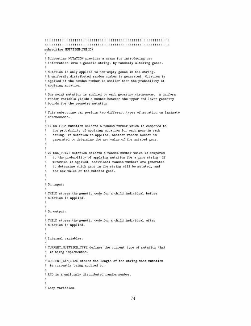
subroutine MUTATION(CHILD)

!

! Subroutine MUTATION provides a means for introducing new

! information into a genetic string, by randomly altering genes.

!

! Mutation is only applied to non-empty genes in the string.

! A uniformly distributed random number is generated. Mutation is

! applied if the random number is smaller than the probability of

! applying mutation.

!

! One point mutation is applied to each geometry chromosome. A uniform

! random variable yields a number between the upper and lower geometry

! bounds for the geometry mutation.

!

! This subroutine can perform two different types of mutation on laminate

! chromosomes.

!

! 1) UNIFORM mutation selects a random number which is compared to

! the probability of applying mutation for each gene in each

! string. If mutation is applied, another random number is

! generated to determine the new value of the mutated gene.

!

!

! 2) ONE_POINT mutation selects a random number which is compared

! to the probability of applying mutation for a gene string. If

! mutation is applied, additional random numbers are generated

! to determine which gene in the string will be mutated, and

! the new value of the mutated gene.

!

!

! On input:

!

! CHILD stores the genetic code for a child individual before

! mutation is applied.

!

!

! On output:

!

! CHILD stores the genetic code for a child individual after

! mutation is applied.

!

!

! Internal variables:

!

! CURRENT_MUTATION_TYPE defines the current type of mutation that

! is being implemented.

!

! CURRENT_LAM_SIZE stores the length of the string that mutation

! is currently being applied to.

!

! RND is a uniformly distributed random number.

!

!

! Loop variables:

74

!

! I,J

!

!

!!!!!!!!!!!!!!!!!!!!!!!!!!!!!!!!!!!!!!!!!!!!!!!!!!!!!!!!!!!!!!!!!

use GENERIC_GA

type(individual), intent(inout) :: child

!Local variables.

real (KIND=R8) :: rnd, temp_digit, new_digit, ub, lb

integer :: i,j,counter

integer :: current_mutation_type,current_lam_size

integer :: temp_orient, temp_material

! Define the different mutation types.

integer, parameter :: UNIFORM = 1, &

ONE_POINT = 2

Lam:do i = 1, individual_attributes%individual_size_lam

call random_number(rnd)

current_mutation_type = individual_attributes% &

laminate_definition_array(i)%mutation_type

if(individual_attributes%laminate_definition_array(i)%empty_plies) &

then

current_lam_size =size( &

pack (child%laminate_array(i)%ply_array, mask = &

child%laminate_array(i)%ply_array%orientation .ne. 0))

else

current_lam_size = individual_attributes% &

laminate_definition_array(i)%laminate_size

end if

select case (current_mutation_type)

case (UNIFORM)

Unif: do j = 1, current_lam_size

call random_number(rnd)

if (rnd < individual_attributes%laminate_definition_array(i) &

%prob_mut_orientation) then

temp_orient = child%laminate_array(i)%ply_array(j)% &

orientation

do

call random_number(rnd)

!Choose a new orientation.

child%laminate_array(i)%ply_array(j)%orientation= &

individual_attributes%laminate_definition_array(i)% &

orientation_array(ceiling(rnd*individual_attributes%&

laminate_definition_array(i)%num_poss_orientations))

if (child%laminate_array(i)%ply_array(j)%orientation /= &

temp_orient) exit

end do

end if

call random_number(rnd)

if (rnd < individual_attributes%laminate_definition_array(i) &

%prob_mut_material) then

temp_material = child%laminate_array(i)%ply_array(j)% &

material

counter=00

do

counter = counter + 1

call random_number(rnd)

75

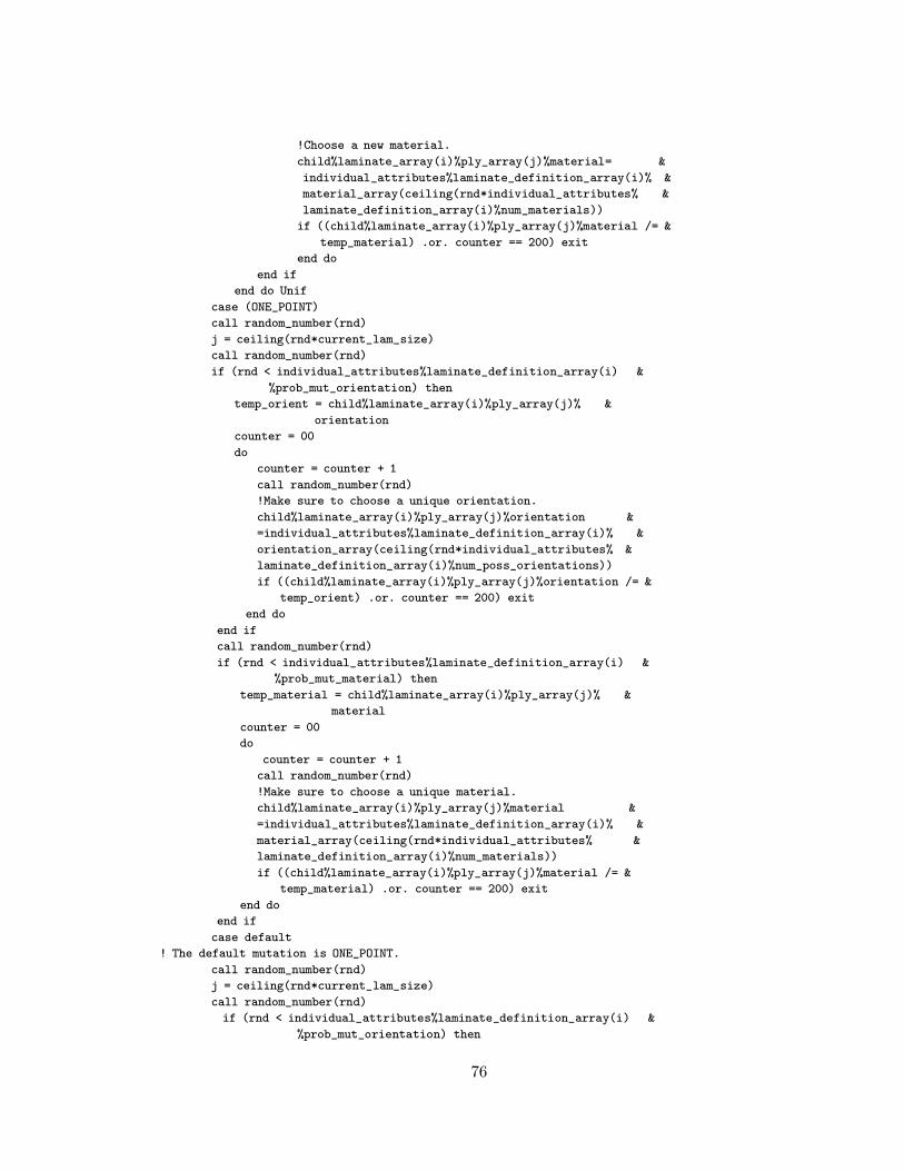
!Choose a new material.

child%laminate_array(i)%ply_array(j)%material= &

individual_attributes%laminate_definition_array(i)% &

material_array(ceiling(rnd*individual_attributes% &

laminate_definition_array(i)%num_materials))

if ((child%laminate_array(i)%ply_array(j)%material /= &

temp_material) .or. counter == 200) exit

end do

end if

end do Unif

case (ONE_POINT)

call random_number(rnd)

j = ceiling(rnd*current_lam_size)

call random_number(rnd)

if (rnd < individual_attributes%laminate_definition_array(i) &

%prob_mut_orientation) then

temp_orient = child%laminate_array(i)%ply_array(j)% &

orientation

counter = 00

do

counter = counter + 1

call random_number(rnd)

!Make sure to choose a unique orientation.

child%laminate_array(i)%ply_array(j)%orientation &

=individual_attributes%laminate_definition_array(i)% &

orientation_array(ceiling(rnd*individual_attributes% &

laminate_definition_array(i)%num_poss_orientations))

if ((child%laminate_array(i)%ply_array(j)%orientation /= &

temp_orient) .or. counter == 200) exit

end do

end if

call random_number(rnd)

if (rnd < individual_attributes%laminate_definition_array(i) &

%prob_mut_material) then

temp_material = child%laminate_array(i)%ply_array(j)% &

material

counter = 00

do

counter = counter + 1

call random_number(rnd)

!Make sure to choose a unique material.

child%laminate_array(i)%ply_array(j)%material &

=individual_attributes%laminate_definition_array(i)% &

material_array(ceiling(rnd*individual_attributes% &

laminate_definition_array(i)%num_materials))

if ((child%laminate_array(i)%ply_array(j)%material /= &

temp_material) .or. counter == 200) exit

end do

end if

case default

! The default mutation is ONE_POINT.

call random_number(rnd)

j = ceiling(rnd*current_lam_size)

call random_number(rnd)

if (rnd < individual_attributes%laminate_definition_array(i) &

%prob_mut_orientation) then

76

temp_orient = child%laminate_array(i)%ply_array(j)% &

orientation

counter = 0

do

counter = counter + 1

call random_number(rnd)

child%laminate_array(i)%ply_array(j)%orientation &

=individual_attributes%laminate_definition_array(i)% &

orientation_array(ceiling(rnd*individual_attributes% &

laminate_definition_array(i)%num_poss_orientations))

if ((child%laminate_array(i)%ply_array(j)%orientation /= &

temp_orient) .or. counter == 200) exit

end do

end if

call random_number(rnd)

if (rnd < individual_attributes%laminate_definition_array(i) &

%prob_mut_material) then

temp_material = child%laminate_array(i)%ply_array(j)% &

material

counter = 00

do

counter = counter + 1

call random_number(rnd)

child%laminate_array(i)%ply_array(j)%material &

=individual_attributes%laminate_definition_array(i)% &

material_array(ceiling(rnd*individual_attributes% &

laminate_definition_array(i)%num_materials))

if ((child%laminate_array(i)%ply_array(j)%material /= &

temp_material) .or. counter == 200) exit

end do

end if

end select

end do Lam

!Apply one point geometry mutation.

Geom:do i = 1, individual_attributes%individual_size_geom

call random_number(rnd)

current_lam_size = individual_attributes%geometry_definition_array(i)%&

geom_chromo_size

j = ceiling(rnd*current_lam_size)

call random_number(rnd)

if (rnd < individual_attributes%geometry_definition_array(i) &

%prob_mutation) then

temp_digit=child%geometry_array(i)%geometry_gene_array(j)%digit

counter = 0

do

counter = counter + 1

ub=individual_attributes%geometry_definition_array(i)% &

upper_bounds_array(j)

lb=individual_attributes%geometry_definition_array(i)% &

lower_bounds_array(j)

call random_number(rnd)

new_digit = min(ub, lb) + rnd*abs(ub-lb)

if (temp_digit /= new_digit .or. ub==lb .or. counter==200) then

child%geometry_array(i)%geometry_gene_array(j)% &

digit = new_digit

exit

77

end if

end do

end if

end do Geom

return

end subroutine MUTATION

!!!!!!!!!!!!!!!!!!!!!!!!!!!!!!!!!!!!!!!!!!!!!!!!!!!!!!!!!!!!!!!!!!

!!!!!!!!!!!!!!!!!!!!!!!!!!!!!!!!!!!!!!!!!!!!!!!!!!!!!!!!!!!!!!!!!!

subroutine DELETION(CHILD)

!

! Subroutine DELETION provides a means of reducing the number of

! genes in a string. Deletion is only applied to laminates which

! allow empty plies, as defined in the variable

! INDIVIDUAL_ATTRIBUTES.

!

! A Uniformly distributed random number is generated for each

! string in a child individual. Deletion is applied if the random

! number is smaller than the probability of applying deletion. If

! deletion is applied, a gene is chosen at random and is converted

! to an empty gene.

!

!

! On input:

!

! CHILD stores the genetic code for a child individual before

! deletion is applied.

!

!

! On output:

!

! CHILD stores the genetic code for a child individual after

! deletion is applied.

!

!

! Internal variables:

!

! CURRENT_LAM_SIZE stores the length of the string that deletion

! is currently being applied to.

!

! J stores the location of the gene to be deleted.

!

! RND is a uniformly distributed random number.

!

!

! Loop variable:

!

! I

!

!

!!!!!!!!!!!!!!!!!!!!!!!!!!!!!!!!!!!!!!!!!!!!!!!!!!!!!!!!!!!!!!!!!!

use GENERIC_GA

type(individual), intent(inout) :: child

!Local variables.

real (KIND=R8) :: rnd

integer :: i, j

integer :: current_lam_size

78

Lam:do i = 1, individual_attributes%individual_size_lam

if(individual_attributes%laminate_definition_array(i)%empty_plies) then

!Check if empty plies are allowed in the current laminate.

current_lam_size =size( &

pack (child%laminate_array(i)%ply_array, mask = &

child%laminate_array(i)%ply_array%orientation .ne. 0))

else

cycle

! Don’t delete if empty plies are not allowed in

! the current laminate.

end if

if (current_lam_size <= 2) then

cycle

! Don’t delete if there are two or less plies in

! the current laminate.

end if

call random_number(rnd)

if (rnd < individual_attributes%laminate_definition_array(i) &

%prob_ply_deletion) then

call random_number(rnd)

j = ceiling(rnd*current_lam_size)

! Make the designated ply empty.

child%laminate_array(i)%ply_array(j)%orientation &

= 0

child%laminate_array(i)%ply_array(j)%material &

= 0

child%laminate_array(i)%ply_array(1:) = &

pack (child%laminate_array(i)%ply_array, mask = &

child%laminate_array(i)%ply_array%orientation .ne. 0, &

vector = (empty_individual%laminate_array(i)%ply_array) )

end if

! End deletion

end do Lam

return

end subroutine DELETION

!!!!!!!!!!!!!!!!!!!!!!!!!!!!!!!!!!!!!!!!!!!!!!!!!!!!!!!!!!!!!!!!!!

!!!!!!!!!!!!!!!!!!!!!!!!!!!!!!!!!!!!!!!!!!!!!!!!!!!!!!!!!!!!!!!!!!

subroutine ADDITION(CHILD)

!

! Subroutine ADDITION provides a means of increasing the number of

! genes in a string. This operator is only applied to laminates

! which allow empty plies, as specified in the variable

! INDIVIDUAL_ATTRIBUTES.

!

! A Uniformly distributed random number is generated for each

! string in a child individual. Addition is applied if the random

! number is smaller than the probability of applying addition. If

! addition is applied, a gene is chosen at random and is converted

! to an empty gene.

!

!

! On input:

!

! CHILD stores the genetic code for a child individual before

! deletion is applied.

!

79

!

! On output:

!

! CHILD stores the genetic code for a child individual after

! deletion is applied.

!

!

! Internal variables:

!

! CURRENT_LAM_SIZE stores the length of the string that deletion

! is currently being applied to.

!

! J stores the location of the gene to be added.

!

! RND is a uniformly distributed random number.

!

!

! Loop variable:

!

! I

!

!

!!!!!!!!!!!!!!!!!!!!!!!!!!!!!!!!!!!!!!!!!!!!!!!!!!!!!!!!!!!!!!!!!!

use GENERIC_GA

type(individual), intent(inout) :: child

!Local variables:

real (KIND=R8) :: rnd

integer :: i, j

integer :: current_lam_size

Lam:do i = 1, individual_attributes%individual_size_lam

if(individual_attributes%laminate_definition_array(i)%empty_plies) &

then

current_lam_size =size( &

pack (child%laminate_array(i)%ply_array, mask = &

child%laminate_array(i)%ply_array%orientation .ne. 0))

else

cycle

! Do not add a gene if the current laminate is of fixed size.

end if

if (current_lam_size == individual_attributes% &

laminate_definition_array(i)%laminate_size) then

cycle

! Do not add a gene if the current laminate is full.

end if

call random_number(rnd)

if (rnd < individual_attributes%laminate_definition_array(i)% &

prob_ply_addition) then

call random_number(rnd)

j = ceiling(rnd*current_lam_size)

child%laminate_array(i)%ply_array(j+1:current_lam_size+1)= &

child%laminate_array(i)%ply_array(j:current_lam_size)

! Add a gene.

child%laminate_array(i)%ply_array(j)%orientation &

=individual_attributes%laminate_definition_array(i)% &

orientation_array(ceiling(rnd*individual_attributes% &

laminate_definition_array(i)%num_poss_orientations))

80

child%laminate_array(i)%ply_array(j)%material &

=individual_attributes%laminate_definition_array(i)% &

material_array(ceiling(rnd*individual_attributes% &

laminate_definition_array(i)%num_materials))

else

end if

end do Lam

return

end subroutine ADDITION

!!!!!!!!!!!!!!!!!!!!!!!!!!!!!!!!!!!!!!!!!!!!!!!!!!!!!!!!!!!!!!!!!!

!!!!!!!!!!!!!!!!!!!!!!!!!!!!!!!!!!!!!!!!!!!!!!!!!!!!!!!!!!!!!!!!!!

subroutine INTRA_PLY_SWAP(CHILD)

!

! Subroutine INTRA_PLY_SWAP provides a means of relaying

! information from one part of a string to another, by randomly

! swapping genes.

!

! A Uniformly distributed random number is generated for each

! string in a child individual. Intra-ply swap is applied if the

! random number is smaller than the probability of applying intra-

! ply swap. If intra-ply swap is applied, the positions of two

! genes in a string are chosen at random and swapped (the values

! of the genes must be unique).

!

!

! On input:

!

! CHILD stores the genetic code for a child individual before

! intra-ply swap is applied.

!

!

! On output:

!

! CHILD stores the genetic code for a child individual after

! intra-ply swap is applied.

!

!

! Internal variables:

!

! CURRENT_LAM_SIZE stores the length of the string that

! intra-ply swap is currently being applied to.

!

! J stores the string position of the first gene to be swapped.

!

! K stores the string position of the second gene to be swapped.

!

! RND is a uniformly distributed random number.

!

! SWAP_1 stores the value of the first gene to be swapped.

!

! SWAP_2 stores the value of the second gene to be swapped.

!

!

! Loop variable:

!

! I

81

!

!

!!!!!!!!!!!!!!!!!!!!!!!!!!!!!!!!!!!!!!!!!!!!!!!!!!!!!!!!!!!!!!!!!!

use GENERIC_GA

type(individual), intent(inout) :: child

!Local variables.

real (KIND=R8):: rnd

integer :: i, j, k, counter

integer :: current_lam_size

integer :: swap_1, swap_2

Lam:do i = 1, individual_attributes%individual_size_lam

if(individual_attributes%laminate_definition_array(i)%empty_plies) then

current_lam_size = size( &

pack(child%laminate_array(i)%ply_array, mask = &

child%laminate_array(i)%ply_array%orientation .ne. 0) )

else

current_lam_size = individual_attributes% &

laminate_definition_array(i)%laminate_size

end if

call random_number(rnd)

if (rnd < individual_attributes%laminate_definition_array(i) &

%prob_intra_ply_swap) then

call random_number(rnd)

j = ceiling(rnd*current_lam_size)

swap_1 = child%laminate_array(i)%ply_array(j)%orientation

counter = 0

do

!Only swap genes which are not identical.

counter = counter + 1

call random_number(rnd)

k = ceiling(rnd*current_lam_size)

if(j /= k) then

swap_2 = child%laminate_array(i)%ply_array(k)%orientation

if(swap_1 /= swap_2 .or. counter >= 200) exit

end if

end do

!Swap the designated genes.

child%laminate_array(i)%ply_array(j)%orientation = swap_2

child%laminate_array(i)%ply_array(k)%orientation = swap_1

swap_1 = child%laminate_array(i)%ply_array(j)%material

swap_2 = child%laminate_array(i)%ply_array(k)%material

child%laminate_array(i)%ply_array(j)%material = swap_2

child%laminate_array(i)%ply_array(k)%material = swap_1

end if

end do Lam

return

end subroutine INTRA_PLY_SWAP

!!!!!!!!!!!!!!!!!!!!!!!!!!!!!!!!!!!!!!!!!!!!!!!!!!!!!!!!!!!!!!!!!!

!!!!!!!!!!!!!!!!!!!!!!!!!!!!!!!!!!!!!!!!!!!!!!!!!!!!!!!!!!!!!!!!!!

subroutine PERMUTATION(CHILD)

!

! Subroutine PERMUTATION provides a means of relaying information

! from one part of a string to another by randomly reordering

! sequence of genes.

!

! A Uniformly distributed random number is generated for each

82

! string in a child individual. Permutation is applied if the

! random number is smaller than the probability of applying

! permutation. If permutaion is applied, the positions of two

! genes in a string are chosen at random. The substring of genes

! defined between and including the two randomly selected

! locations is then inverted

! (e.g., [1,2,3,4] -> [4,3,2,1]).

!

!

! On input:

!

! CHILD stores the genetic code for a child individual before

! permutation is applied.

!

!

! On output:

!

! CHILD stores the genetic code for a child individual after

! permutation is applied.

!

!

! Internal variables:

!

! CURRENT_LAM_SIZE stores the length of the string that

! permutation is currently being applied to.

!

! J stores the string position of the left end of the permutation

! string.

!

! K stores the string position of the right end of the permutation

! string.

!

! PERMUTATION_ARRAY stores the gene values in the permutation

! string.

!

! RND is a uniformly distributed random number.

!

! STRING_LENGTH stores the number of genes in the permutation

! string.

!

!

! Loop variable:

!

! I

!

!

!!!!!!!!!!!!!!!!!!!!!!!!!!!!!!!!!!!!!!!!!!!!!!!!!!!!!!!!!!!!!!!!!!

use GENERIC_GA

type(individual), intent(inout) :: child

!Local variables.

real (KIND=R8):: rnd

integer :: i, j, k, temp

integer :: current_lam_size, string_length

integer, dimension(:), allocatable :: permutation_array

Lam: do i = 1, individual_attributes%individual_size_lam

allocate(permutation_array(2*individual_attributes% &

83

laminate_definition_array(i)%laminate_size))

if(individual_attributes%laminate_definition_array(i)%empty_plies) then

current_lam_size = size( &

pack(child%laminate_array(i)%ply_array, mask = &

child%laminate_array(i)%ply_array%orientation .ne. 0) )

else

current_lam_size = individual_attributes% &

laminate_definition_array(i)%laminate_size

end if

call random_number(rnd)

if (rnd < individual_attributes%laminate_definition_array(i) &

%prob_permutation) then

call random_number(rnd)

j = ceiling(rnd*current_lam_size)

do

call random_number(rnd)

k = ceiling(rnd*current_lam_size)

if(j /= k) exit

end do

if (j > k) then

!Ensure that k > j.

temp = j

j = k

k = temp

end if

string_length = k - j + 1

permutation_array(1:string_length) = &

child%laminate_array(i)%ply_array(j:k)%orientation

permutation_array(string_length+1:2*string_length) = &

child%laminate_array(i)%ply_array(j:k)%material

child%laminate_array(i)%ply_array(j:k)%orientation = &

permutation_array(string_length:1:-1)

child%laminate_array(i)%ply_array(j:k)%material = &

permutation_array(2*string_length:string_length+1:-1)

end if

deallocate(permutation_array)

end do Lam

return

end subroutine PERMUTATION

!!!!!!!!!!!!!!!!!!!!!!!!!!!!!!!!!!!!!!!!!!!!!!!!!!!!!!!!!!!!!!!!!!!

!!!!!!!!!!!!!!!!!!!!!!!!!!!!!!!!!!!!!!!!!!!!!!!!!!!!!!!!!!!!!!!!!!!

real function RNOR()

!

!

integer :: iseed

real :: vni

!***begin prologue rnor

!***date written 810915 (yymmdd)

!***revision date 870419 (yymmdd)

!***category no. l6a14

!***keywords random numbers, normal deviates

!***author kahaner, david, scientific computing division, nbs

! marsaglia, george, supercomputer res. inst., florida st. u.

!

!***purpose generates normal random numbers, with mean zero and

! unit standard deviation, often denoted n(0,1).

84

!***description

!

! rnor generates normal random numbers with zero mean and

! unit standard deviation, often denoted n(0,1).

! from the book, "numerical methods and software" by

! d. kahaner, c. moler, s. nash

! prentice hall, 1988

! use

! first time....

! z = rstart(iseed)

! here iseed is any n o n - z e r o integer.

! this causes initialization of the program.

! rstart returns a real (single precision) echo of iseed.

!

! subsequent times...

! z = rnor()

! causes the next real (single precision) random number

! to be returned as z.

!

!.....................................................................

! typical usage

!

! real rstart,rnor,z

! integer iseed,i

! iseed = 305

! z = rstart(iseed)

! do 1 i = 1,10

! z = rnor()

! write(*,*) z

! 1 continue

! end

!

!

!***references marsaglia & tsang, "a fast, easily implemented

! method for sampling from decreasing or

! symmetric unimodal density functions", to be

! published in siam j sisc 1983.

!***routines called (none)

!***end prologue rnor

real aa,b,c,c1,c2,pc,x,y,xn,v(65),rstart,u(17),s,t,un

integer j,ia,ib,ic,ii,jj,id,iii,jjj

save u,ii,jj

!

data aa,b,c/12.37586,.4878992,12.67706/

data c1,c2,pc,xn/.9689279,1.301198,.1958303e-1,2.776994/

data v/ .3409450, .4573146, .5397793, .6062427, .6631691 &

, .7136975, .7596125, .8020356, .8417227, .8792102, .9148948 &

, .9490791, .9820005, 1.0138492, 1.0447810, 1.0749254, 1.1043917 &

,1.1332738, 1.1616530, 1.1896010, 1.2171815, 1.2444516, 1.2714635 &

,1.2982650, 1.3249008, 1.3514125, 1.3778399, 1.4042211, 1.4305929 &

,1.4569915, 1.4834526, 1.5100121, 1.5367061, 1.5635712, 1.5906454 &

,1.6179680, 1.6455802, 1.6735255, 1.7018503, 1.7306045, 1.7598422 &

,1.7896223, 1.8200099, 1.8510770, 1.8829044, 1.9155830, 1.9492166 &

,1.9839239, 2.0198430, 2.0571356, 2.0959930, 2.1366450, 2.1793713 &

,2.2245175, 2.2725185, 2.3239338, 2.3795007, 2.4402218, 2.5075117 &

,2.5834658, 2.6713916, 2.7769943, 2.7769943, 2.7769943, 2.7769943/

85

! load data array in case user forgets to initialize.

! this array is the result of calling uni 100000 times

! with seed 305.

data u/ &

0.8668672834288, 0.3697986366357, 0.8008968294805, &

0.4173889774680, 0.8254561579836, 0.9640965269077, &

0.4508667414265, 0.6451309529668, 0.1645456024730, &

0.2787901807898, 0.06761531340295, 0.9663226330820, &

0.01963343943798, 0.02947398211399, 0.1636231515294, &

0.3976343250467, 0.2631008574685/

!

data ii,jj / 17, 5 /

!

!***first executable statement rnor

!

! fast part...

!

!

! basic generator is fibonacci

!

un = u(ii)-u(jj)

if(un.lt.0.0) un = un+1.

u(ii) = un

! u(ii) and un are uniform on [0,1)

! vni is uniform on [-1,1)

vni = un + un -1.

ii = ii-1

if(ii.eq.0)ii = 17

jj = jj-1

if(jj.eq.0)jj = 17

! int(un(ii)*128) in range [0,127], j is in range [1,64]

j = mod(int(u(ii)*128),64)+1

! pick sign as vni is positive or negative

rnor = vni*v(j+1)

if(abs(rnor).le.v(j))return

!

! slow part; aa is a*f(0)

x = (abs(rnor)-v(j))/(v(j+1)-v(j))

! y is uniform on [0,1)

y = u(ii)-u(jj)

if(y.lt.0.0) y = y+1.

u(ii) = y

ii = ii-1

if(ii.eq.0)ii = 17

jj = jj-1

if(jj.eq.0)jj = 17

!

s = x+y

if(s.gt.c2)go to 11

if(s.le.c1)return

if(y.gt.c-aa*exp(-.5*(b-b*x)**2))go to 11

if(exp(-.5*v(j+1)**2)+y*pc/v(j+1).le.exp(-.5*rnor**2))return

!

! tail part; .3601016 is 1./xn

! y is uniform on [0,1)

22 y = u(ii)-u(jj)

86

if(y.le.0.0) y = y+1.

u(ii) = y

ii = ii-1

if(ii.eq.0)ii = 17

jj = jj-1

if(jj.eq.0)jj = 17

!

x = 0.3601016*log(y)

! y is uniform on [0,1)

y = u(ii)-u(jj)

if(y.le.0.0) y = y+1.

u(ii) = y

ii = ii-1

if(ii.eq.0)ii = 17

jj = jj-1

if(jj.eq.0)jj = 17

if( -2.*log(y).le.x**2 )go to 22

rnor = sign(xn-x,rnor)

return

11 rnor = sign(b-b*x,rnor)

return

!

!

! fill

entry rstart(iseed)

if(iseed.ne.0) then

!

! set up ...

! generate random bit pattern in array based on given seed

!

ii = 17

jj = 5

ia = mod(abs(iseed),32707)

ib = 1111

ic = 1947

do iii = 1,17

s = 0.0

t = .50

! do for each of the bits of mantissa of word

! loop over 64 bits, enough for all known machines

! in single precision

do jjj = 1,64

id = ic-ia

if(id.ge.0)goto 4

id = id+32707

s = s+t

4 ia = ib

ib = ic

ic = id

t = .5*t

end do

u(iii) = s

end do

endif

! return floating echo of iseed

rstart=iseed

87

return

end function

!

!!!!!!!!!!!!!!!!!!!!!!!!!!!!!!!!!!!!!!!!!!!!!!!!!!!!!!!!!!!!!!!!!!

88

B.3 Genetic Algorithm Selection Schemes.

subroutine ELITIST_SELECTION()

!

! Subroutine ELITIST_SELECTION is a selection routine then ensures that

! the GA converges to an optimal design by retaining the best individuals

! from generation to generation. All individuals except the least fit

! are copied from CHILD_POP into PARENT_POP, while the most fit individual in

! PARENT_POP is kept in PARENT_POP.

!

! On input:

!

! PARENT_POP is the parent population from the previous generation, of

! type (popltn).

!

! CHILD_POP is the child population from the previous generation, of

! type (popltn).

!

!

! On output:

!

! PARENT_POP contains the most fit individual of the original PARENT_POP

! and all but the least fit individuals from the original CHILD_POP.

!

!!!!!!!!!!!!!!!!!!!!!!!!!!!!!!!!!!!!!!!!!!!!!!!!!!!!!!!!!!!!!!!!!!!!!!!!!!

!Local variables:

integer :: I , subpop

type (individual) :: temp

pop:do subpop = 1, population_size

! Keep the best parent.

if (parent_rank_array(subpop,1) /= 1) then

temp = population%subpopulation_array(subpop)%individual_array(1)

population%subpopulation_array(subpop)%individual_array(1) = &

population%subpopulation_array(subpop)%individual_array( &

parent_rank_array(subpop,1))

population%subpopulation_array(subpop)%individual_array( &

parent_rank_array(subpop,1)) = temp

parent_fitness_array(subpop,1)=parent_fitness_array(subpop, &

parent_rank_array(subpop,1))

end if

! Keep children ranked 1...(subpopulation_size-1).

ILoop:do I = 1, (subpopulation_size-1)

temp = population%subpopulation_array(subpop)%individual_array(I+1)

population%subpopulation_array(subpop)%individual_array(I+1)= &

child_population%subpopulation_array(subpop)%individual_array( &

child_rank_array(subpop,I))

child_population%subpopulation_array(subpop)%individual_array( &

child_rank_array(subpop,I))=temp

! Store fitness to prevent re-analysis

parent_fitness_array(subpop,I+1)=child_fitness_array(subpop, &

child_rank_array(subpop,I))

end do ILoop

end do pop

return

end subroutine ELITIST_SELECTION

!!!!!!!!!!!!!!!!!!!!!!!!!!!!!!!!!!!!!!!!!!!!!!!!!!!!!!!!!!!!!!!!!!!!!!!!!!

89

subroutine MULTIPLE_ELITIST2_SELECTION()

!

! Subroutine MULTIPLE_ELITIST2_SELECTION is a selection routine then ensures

! that the GA converges to an optimal design by retaining the Nk best

! members from the combined parent and child population. They are stored

! in population, while the rest of the places in population are the

! best from the child population that have not already been used.

!

! On input:

!

! population is the parent population from the previous generation, of

! type (popltn).

!

! child_population is the child population from the previous generation, of

! type (popltn).

!

!

! On output:

!

! population contains the most fit individuals of the combined populations

! and all but the least fit individuals from the original child_population.

!

!!!!!!!!!!!!!!!!!!!!!!!!!!!!!!!!!!!!!!!!!!!!!!!!!!!!!!!!!!!!!!!!!!!!!!!!!!

!Local variables:

integer :: subpop, I, J, K

type (individual) :: temp

type (individual) :: temp_ind

double precision :: temp_fitness

integer :: swaps

swaps = 0

pop:do subpop = 1, population_size

ILoop:do I = 1, nk

JLoop:do J= 1, subpopulation_size

if (child_fitness_array(subpop,child_rank_array(subpop,J)) > parent_fitness_array(subpop,

&

parent_rank_array(subpop,I))) then

temp_ind = &

population%subpopulation_array(subpop)%individual_array(parent_rank_array(subpop,I))

population%subpopulation_array(subpop)%individual_array(parent_rank_array(subpop,I))= &

child_population%subpopulation_array(subpop)%individual_array( &

child_rank_array(subpop, J))

child_population%subpopulation_array(subpop)%individual_array( &

child_rank_array(subpop, J)) = temp_ind

swaps = swaps + 1

temp_fitness =parent_fitness_array(subpop, parent_rank_array(subpop,I))

parent_fitness_array(subpop,parent_rank_array(subpop,I))=child_fitness_array(subpop,

child_rank_array(subpop,J))

child_fitness_array(subpop,child_rank_array(subpop, J)) = temp_fitness

exit

endif

end do JLoop

end do ILoop

KLoop:do K = nk+1, subpopulation_size

temp_ind = &

population%subpopulation_array(subpop)%individual_array(parent_rank_array(subpop,K))

population%subpopulation_array(subpop)%individual_array(parent_rank_array(subpop,K))= &

90

child_population%subpopulation_array(subpop)%individual_array( &

child_rank_array(subpop,swaps+ K - nk))

child_population%subpopulation_array(subpop)%individual_array( &

child_rank_array(subpop,swaps+ K - nk)) = temp_ind

! Store fitness to prevent re-analysis

parent_fitness_array(subpop,parent_rank_array(subpop,K))= &

child_fitness_array(subpop, child_rank_array(subpop,swaps+K -nk))

end do KLoop

end do pop

return

end subroutine MULTIPLE_ELITIST2_SELECTION

!!!!!!!!!!!!!!!!!!!!!!!!!!!!!!!!!!!!!!!!!!!!!!!!!!!!!!!!!!!!!!!!!!!!!!!!!!

subroutine MULTIPLE_ELITIST1_SELECTION()

!

! Subroutine MULTIPLE_ELITIST1_SELECTION is a selection routine then ensures

! that the GA converges to an optimal design by retaining the Nk best

! members from the parent. They are stored

! in population, while the rest of the places in population are the

! best from the child population.

!

! On input:

!

! population is the parent population from the previous generation, of

! type (popltn).

!

! child_population is the child population from the previous generation, of

! type (popltn).

!

!

! On output:

!

! population contains the most fit individuals of the combined populations

! and all but the least fit individuals from the original child_population.

!

!!!!!!!!!!!!!!!!!!!!!!!!!!!!!!!!!!!!!!!!!!!!!!!!!!!!!!!!!!!!!!!!!!!!!!!!!!

!Local variables:

integer :: subpop, counter1, I, J

type (individual) :: temp

type (individual), dimension(nk) :: temp_population

type (individual) :: temp_ind

double precision, dimension(nk) :: temp_fitnesses

pop:do subpop = 1, population_size

! Keep children ranked 1...(subpopulation_size-Nk).

ILoop:do I = nk+1, subpopulation_size

temp_ind = &

population%subpopulation_array(subpop)%individual_array(parent_rank_array(subpop,I))

population%subpopulation_array(subpop)%individual_array(parent_rank_array(subpop,I))= &

child_population%subpopulation_array(subpop)%individual_array( &

child_rank_array(subpop,I-nk))

child_population%subpopulation_array(subpop)%individual_array( &

child_rank_array(subpop,I-nk)) = temp_ind

! Store fitness to prevent re-analysis

parent_fitness_array(subpop,parent_rank_array(subpop,I))= &

child_fitness_array(subpop, child_rank_array(subpop,I-nk))

end do ILoop

end do pop

91

return

end subroutine MULTIPLE_ELITIST1_SELECTION

92

VITA.

Matthew T. McMahon was born on August 30, 1968, in Miami, Florida. He earned

a Bachelor of electrical engineering degree from Auburn University in 1990, after which

he was employed as an engineer with the General Electric Company. In August, 1998, he

received the MS degree in computer science from Virginia Polytechnic Institute and State

University. He will attend University of Virginia School of Medicine, and hopes to apply

his engineering and computer science background in the realm of medical informatics.

93