A discontinuous Galerkin method for two-dimensional flow and transport in shallow water

A discontinuous Galerkin method for two-dimensional flow andtransport in shallow water

Vadym Aizinger, Clint Dawson *,1

Center for Subsurface Modeling, C0200, Texas Institute for Computational and Applied Mathematics, The University of Texas at Austin, Austin,

TX 78712, USA

Received 20 December 2000; received in revised form 26 April 2001; accepted 1 May 2001

Abstract

A discontinuous Galerkin (DG) finite element method is described for the two-dimensional, depth-integrated shallow water

equations (SWEs). This method is based on formulating the SWEs as a system of conservation laws, or advection–diffusion

equations. A weak formulation is obtained by integrating the equations over a single element, and approximating the unknowns by

piecewise, possibly discontinuous, polynomials. Because of its local nature, the DG method easily allows for varying the polynomial

order of approximation. It is also ‘‘locally conservative’’, and incorporates upwinded numerical fluxes for modeling problems with

high flow gradients. Numerical results are presented for several test cases, including supercritical flow, river inflow and standard

tidal flow in complex domains, and a contaminant transport scenario where we have coupled the shallow water flow equations with

a transport equation for a chemical species. � 2002 Elsevier Science Ltd. All rights reserved.

Keywords: Shallow water equations; Discontinuous Galerkin method

1. Introduction

The two-dimensional shallow water equations(SWEs) are used to describe flow in vertically well-mixedwater bodies where the horizontal length scales aremuch greater than the fluid depth (i.e., long wavelengthphenomena). The SWEs are obtained by assuming ahydrostatic pressure distribution and a uniform velocityprofile in the vertical direction. By integrating theNavier–Stokes equations along the depth of the fluidbody, the three-dimensional free boundary problem re-duces to a two-dimensional fixed boundary problemwith the primary variables being the vertical averages ofthe horizontal fluid velocities and the fluid depth (see[22] for a derivation of the SWEs). The SWEs can beused to study many physical phenomena of interest,such as storm surges, tidal fluctuations, tsunami waves,forces acting on off-shore structures, and can be coupled

to transport equations to model transport of chemicalspecies.The numerical solution of the SWEs is made

challenging by a number of factors. The SWEs are asystem of coupled non-linear partial differentialequations defined on complex physical domains aris-ing, for example, from irregular land boundaries. Thebottom sea bed (bathymetry) is also often very irreg-ular. Shallow water systems are subjected to a widevariety of external forces, such as the Coriolis force,the surface wind stress, atmospheric pressure gradient,and tidal potential forces. In addition to these physicalfactors, there are additional difficulties arising fromthe mathematical nature of the SWEs. Most importantis the coupling between the fluid depth and the hori-zontal velocity field which could lead to spuriousspatial oscillations if the numerical algorithms are notchosen with care.Most numerical algorithms which have been devel-

oped for the SWEs over the years can be classified intotwo broad categories. In the first category, the primitiveform of the SWEs that are obtained from the directvertical integration of the three-dimensional incom-pressible Navier–Stokes equations, are numericallysolved. In this case, a straightforward use of equal-order

Advances in Water Resources 25 (2002) 67–84

www.elsevier.com/locate/advwatres

*Corresponding author. Tel.: +1-512-475-8627; fax: +1-512-471-86-

94.

E-mail address: [email protected] (C. Dawson).1 This work was funded by the National Science Foundation, Project

No. DMS-9873326 and DMS-9805491.

0309-1708/02/$ - see front matter � 2002 Elsevier Science Ltd. All rights reserved.

PII: S0309 -1708 (01)00019 -7

interpolation spaces in the finite element context or theuse of non-staggered grids in the finite difference contextcan lead to spurious spatial oscillations [18]. Over theyears, various researchers have attempted to controlthese oscillations through the use of staggered grids ormixed interpolation spaces, with limited success. Forexample, King and Norton [16] approximate velocitiesthrough piecewise quadratic functions and elevationsusing piecewise linear functions. Johnson et al. [13] andBlumberg and Mellor [3] utilize logically rectangulargrids, with velocities defined on the edges of the elementsand elevation defined at the element centers. Severalnumerical methods based on the primitive SWEs andequal order approximations have also been developed(e.g., [15, 20, 23]) which utilize various techniques forcontrolling oscillations. For example, the approach ofZienkiewicz and Ortiz [23] uses a special operatorsplitting combined with a method of characteristics. Inthe second category, the primitive SWEs are reformu-lated and the first-order hyperbolic form of the primitivecontinuity equation is replaced with a second-orderwave equation (see, for example, [17,18]).We have taken a slightly different view of the SWEs.

In particular, the SWEs can be expressed as a system ofconservation laws, or as advection–diffusion equations ifdiffusive effects such as eddy viscosity are incorporated.In an earlier paper, we approximated the non-viscidsystem using a Godunov-type method defined on tri-angular elements [4]. This approach used discontinuous,piecewise constant approximations of elevation and ve-locity. A similar method defined on rectangular elementswas described by Alcrudo and Garcia-Navarro [2] forthe SWEs. In this type of approach, one can make themethod ‘‘higher-order’’ through a post-processing stepwhereby linear terms are added to the solution on eachelement. In [4], after testing several different post-pro-cessing algorithms, we devised a method based on lin-earizing the system on each element and decoupling theresulting equations. Linear terms (x and y ‘‘slopes’’)were constructed for the elevation variable, then theseslopes were used to enhance the velocity approximationderived from the linearized equations. While this ap-proach gave better accuracy and sharper resolution ofthe solution for some test problems, it was very ad hocin nature, and did not always work well in practice.In this paper, we describe a discontinuous Galerkin

(DG) method for the SWEs. This approach generalizesand extends the Godunov method described in [4] inseveral ways. First, the use of higher-order polynomialsis naturally built into the method; instead of computingthese higher-order terms through some sort of ad hocpost-processing procedure, they are defined through thevariational equation. Second, diffusive terms can be in-corporated into the method; the Godunov methodprovides no mechanism for dealing with second-orderderivatives. Furthermore, though we do not emphasize

it here, the DG method allows for the use of non-con-forming grids; i.e., grids with non-matching faces,without the use of hanging nodes or mortar spaces. Thisfeature could be very useful in dealing with complicatedgeometries and adaptive meshes. Compared to themethods described above, DG methods are based on theprimitive SWEs with equal-order spaces but have built-in mechanisms for capturing shocks or sharp fronts andminimizing oscillations, and also are based on satisfyingthe continuity and momentum equations element-by-element. This last property is useful, for example, whencoupling a shallow water flow simulator to a contami-nant transport model. We will discuss such couplings ina later section.The DG method we describe here is based on the so-

called local discontinuous Galerkin (LDG) method, firstanalyzed by Cockburn and Shu [8]. This method in turnwas an extension of the Runge–Kutta DG method forconservation laws described and analyzed by Cockburnand Shu in a series of papers [6,7,9–11]. Cockburn andShu proved stability of the LDG method for non-linearadvection–diffusion systems, and derived a priori errorestimates for constant coefficient problems. Cockburnand Dawson generalized these results to multi-dimen-sional equations with spatially varying coefficients in [5].In collaboration with Cockburn and Castillo, we havealso applied the LDG method to contaminant transportequations arising in porous media [1].In Section 2, the mathematical model is described,

and in Section 3, the LDG method is formulated. InSection 4, the method is applied to several test cases,including supercritical flow through a constrictedchannel, tidal flow near the Bahamas Islands, contami-nant transport in Galveston Bay, and river inflow intothe Gulf of Mexico. Finally, in Section 5, we give someconclusions.

2. Mathematical model

Vertical integration of the Navier–Stokes equationsalong with the assumptions of a hydrostatic pressureand a vertically uniform horizontal velocity profile re-sults in the shallow water equations (SWEs) of the fol-lowing form:

onot

þr � uHð Þ ¼ 0; ð1Þ

ou

otþ u � ruþ sbfuþ fck� uþ grn � mT

HDðHuÞ

¼ 1

HF: ð2Þ

Eq. (1) represents the conservation of mass and is alsoreferred to as the primitive continuity equation; Eq. (2)represents the conservation of momentum in non-con-servative form. In the above equations, n represents the

68 V. Aizinger, C. Dawson / Advances in Water Resources 25 (2002) 67–84

deflection of the air–liquid interface from the mean sealevel, H ¼ hb þ n represents the total fluid depth, and hbis the bathymetric depth (see Fig. 1), u ¼ ðu; vÞ is thedepth averaged horizontal velocity field, fc is the Cori-olis parameter resulting from the earth’s rotation, k isthe local vertical vector, g is the gravitational accelera-tion, sbf is the bottom friction coefficient, and mT is thedepth averaged turbulent viscosity. We have used theform of the diffusion term as given in [17]. In addition tothe above described phenomena, often we need to in-clude the effects of surface wind stress, variable at-mospheric pressure and tidal potentials which areexpressed through the body force F [22]. The conserva-tive form of the momentum equation can be derived bymultiplying (2) by H , and combining (1) and (2), re-sulting in

oq

otþr � qqT=H

� �þ sbfq

þ fck� qþ gHrn � mTDq ¼ F; ð3Þ

where q ðU ; V Þ uH . Thus, the continuity equation(1) along with the non-conservative momentum equa-tion (2) or the conservative momentum equation (3)represent the SWEs in the primitive form and are solved,usually numerically, for n and u or q.The system of SWEs given by (1) and (3) can be re-

written in the following compact vector form:

oc

otþr � ðA� DrcÞ ¼ hðcÞ; ð4Þ

where

c ¼nUV

0@

1A;

A ¼U V

U2

H þ 12g H 2 � h2b� �

UVH

UVH

V 2

H þ 12g H 2 � h2b� �

0@

1A; ð5Þ

D ¼0 0 0

0 mTI 00 0 mTI

24

35 ð6Þ

and

hðcÞ ¼0

�sbfU þ fcV þ gn ohbox þ Fx

�sbfV � fcU þ gn ohboy þ Fy

0B@

1CA: ð7Þ

The matrix D has a block structure where 0 is the 2� 2zero matrix and I is the 2� 2 identity matrix. The pri-mary variables are n and ðU ; V Þ. Fx; Fy

� �are the ad-

ditional body forces arising from wind stress,atmospheric pressure gradient, tide potential, etc.The above equations are defined over a spatial do-

main X and for t > 0. Let n denote the unit outwardnormal to oX. In the inviscid case (mT ¼ 0), the bound-ary conditions for the SWEs are assumed to be one offollowing types:

Land boundary. At a land boundary we assume

u � n ¼ 0; ð8ÞRiver boundary. River boundaries bring flow into thesystem. We assume,

u � n ¼ uu � n; n ¼ nn; ð9Þwhere uu and nn are specified.

Open-sea boundary. At an open-sea boundary condition,we assume

n ¼ nn; ð10Þwhere nn is again specified. We may also impose a radi-ation-type boundary condition.When mT > 0, additional boundary conditions must

be specified.The initial conditions are given by

nðx; 0Þ ¼ n0ðxÞ; uðx; 0Þ ¼ u0ðxÞ: ð11ÞIn geophysical flow simulations, the initial conditions areoften impossible to measure, and in such instances a coldstart simulation is performed. In cold start simulations,the fluid domain is assumed to be at rest initially (n0 ¼ 0,u0 ¼ 0) and the boundary conditions and forcing func-tions are applied gradually through ramp functions.

3. The LDG method

Before describing the LDG method for (4) we definesome notation. On any spatial domain R let ð�; �ÞR denotethe L2ðRÞ inner product. To distinguish integration overdomains R 2 Rd�1 (e.g., surfaces or lines), we will use thenotation h�; �iR. Let fThgh>0 denote a family of finiteelement partitions of X such that no element Xe crossesthe boundary of X, where h is the maximal element di-ameter. Let

Wh;e ¼ fw : each component of w is a polynomial of

degree 6 ke on Xe 2 Thg:

Fig. 1. Definition of elevation and bathymetry.

V. Aizinger, C. Dawson / Advances in Water Resources 25 (2002) 67–84 69

We do not specify here the number of components in wand below it may vary depending on the variable we areapproximating. Note that the degree ke could vary fromone element to the next. Let ne denote the unit outwardnormal to @Xe. Then, for x 2 @Xe we define

wintðxÞ ¼ lims!0�

wðxþ sneÞ;

and

wextðxÞ ¼ lims!0þ

wðxþ sneÞ:

That is, wint is the value of w from the interior of Xe andwext is the value of w from the exterior of Xe. We alsodefine

w ¼ ðwint þ wextÞ=2: ð12ÞThe LDG method is based on the following mixed

form of (4). Define

~zz ¼ �ð0;rU ;rV Þ ð13Þand

z ¼ D~zz: ð14ÞThen substituting z into (4), multiplying by a sufficientlysmooth test function w, and integrating over an elementXe, we obtain

oc

ot;w

�Xe

� Að þ z;r � wÞXe þ hðAþ zÞ � ne;wintioXe

¼ hðcÞ;wð ÞXe : ð15Þ

Multiplying (13) by a suitable test function ~vv and inte-grating we find

ð~zz;~vvÞXe � ðc;r � ~vvÞXe þ hc;~vvint � neioXe ¼ 0 ð16Þ

and multiplying (14) by a test function v and integratingwe obtain

ðz; vÞXe � ðD~zz; vÞXe ¼ 0: ð17Þ

We approximate c;~zz and z by functions C; ~ZZ and Z inWh;e. We also approximate A � ne on oXe by a numericalflux AAðCint;Cext; neÞ, which we will discuss below. Allother boundary terms are approximated by averaging.Thus, the DG method is given by

oC

ot;w

�Xe

� AðCÞð þ Z;r � wÞXe

þ hAAðCint;Cext; neÞ þ Z � ne;wintioXe¼ hðCÞ;wð ÞXe ; w 2 Wh;e; ð18Þ

ð~ZZ;~vvÞXe � ðC;r � ~vvÞXe þ hC;~vvint � neioXe ¼ 0;~vv 2 Wh;e; ð19Þ

ðZ; vÞXe � ðD~ZZ; vÞXe ¼ 0; v 2 Wh;e: ð20Þ

We now make some remarks concerning the method.1. From (20), we can express Z in terms of ~ZZ, and ~ZZ inturn can be expressed in terms of C by (19). Substitut-

ing into (18) we obtain a problem in C unknownsalone. Thus, Z and ~ZZ are only defined for mathemat-ical convenience.

2. The method is ‘‘locally conservative’’ in the followingsense. Letting w ¼ 1 on Xe and zero elsewhere,

oC

ot; 1

�Xe

þ hAAðCint;Cext; neÞ þ Z � ne; 1ioXe

¼ hðCÞ; 1ð ÞXe : ð21Þ

Thus, the rate of change of C integrated over Xe isbalanced by advective and diffusive fluxes, and sourceterms.

3. The only interaction between the unknowns on Xe

and those on neighboring elements occurs throughboundary integrals. We do not require that the el-ement boundaries align. Thus, one can have mesheswhich are non-conforming. Moreover, the shape ofXe can be very general. From a mathematical stand-point, the only requirement we impose is that theboundary of Xe should be Lipschitz [5].

4. The numerical flux AA can be any locally Lipschitz,conservative, consistent, entropy flux. By conserva-tive, we mean that

AAðCint;Cext; neÞ þ AAðCext;Cint;�neÞ ¼ 0 ð22Þ

and by consistent, we mean that

AAðC;C; neÞ ¼ AðCÞ � ne: ð23Þ

In the numerical calculations below, we have used aRoe flux approximation [19], described in detail in [4].

5. The boundary conditions (8)–(10) are used in con-structing an appropriate exterior state Cext on thoseboundaries oXe which intersect oX. At a land bound-ary, given Cint and normal and tangent vectors n ands, we compute

qintn qint � n;qints qint � s

and given H int, we can compute an approximationuintn ¼ qintn =H int and similarly obtain uints . We set

uextn ¼ �uintn ;

in accordance with (10). We approximate uexts and H ext

by

uexts ¼ uints ;

H ext ¼ H int:

We then compute qextn ¼ uextn H ext, qexts , and from thesequantities and H ext, we obtain Cext. At an open-seaboundary, the exterior state H ext is computed usingthe specified elevation nn and qext ¼ qint. At river inflowboundaries, H ext and qext are computed using theknown river inflows. Finally, at radiation boundaries,we set Cext ¼ Cint.


6. The system (18)–(20) is discretized in time using ex-plicit Runge–Kutta procedures as described in[6,7,9–11]. Here it was demonstrated that by choosingappropriate coefficients, first-, second- and third-or-der Runge–Kutta methods can be developed whichare TVD (total variation diminishing) when appliedto the time evolution of conservation laws, under cer-tain CFL constraints. For our problem, since diffu-sion is included, the time step constraint is of theform

Dt6 min minXe

heðkmaxÞe

;minXe

h2emT

�; ð24Þ

where he is the diameter of element Xe, and kmax is themaximum eigenvalue of the Jacobian of the numericalflux A � ne. These eigenvalues are given byu � ne �

ffiffiffiffiffiffiffigH

p; u � ne, and u � ne þ

ffiffiffiffiffiffiffigH

p. Thus the maxi-

mum eigenvalue is computed on each edge, and themaximum over all edges of Xe is used to computeðkmaxÞe.We have implemented and tested constant, linear and

quadratic approximations C on triangular elements Xe.For the case of constants, the scheme (18) with mT ¼ 0 isprecisely the same as the method described in our earlierpaper [4]. First-order Runge–Kutta (explicit Euler) isused for temporal integration in this case. When usinglinear approximations, second-order Runge–Kutta isused for the temporal integration, and for quadraticapproximations, a third order Runge–Kutta method isused. In order to prevent non-physical oscillations, it issometimes necessary to perform stability post-process-ing at each stage of the Runge–Kutta procedure. Es-sentially, this is a slope-limiting method used to modifythe coefficients in the higher-order terms to suppressovershoot and undershoot in the solution. A procedurefor performing this limiting on triangular meshes is de-scribed in [6]. We have found that for a number of cases,we have been able to use higher order approximationswithout slope-limiting and have not had difficulties. Thiswas not the case with the ad hoc reconstruction methoddescribed in our earlier paper [4]. The difference may liein the fact that the higher-order terms are computed aspart of the finite element scheme, and not through somesort of finite difference method.

4. Species transport

As noted above, the SWEs may be coupled to speciestransport equations, for example, salinity or tempera-ture transport or the transport of some contaminant.Let s denote the concentration of the species. Assumings is vertically uniform and, for simplicity, neglectingdiffusive effects, then by integrating the transport equa-tion over the vertical we obtain the two-dimensionaladvection equation

oðsHÞot

þr � ðqsÞ ¼ g; ð25Þ

where g represents a source term. Appropriate initialand boundary conditions on s must also be given.Given approximations to H and q, we can apply the

DG method described above to approximate s. In [1,5],we describe how to apply the LDGmethod to such typesof transport equations. In [12], we also demonstrate thatwhen using a locally conservative method for transport,it is important to use locally conservative elevations andvelocities; in particular, elevations and velocities whichsatisfy (1) in a weak sense over each element. Otherwise,spurious sources/sinks may be added to the solution.Briefly, multiplying (25) by a test function w and in-

tegrating over Xe, we obtain

oðsHÞot

;w �

Xe

� ðsq;rwÞXe þ hsq � ne;wintioXe

¼ ðg;wÞXe : ð26Þ

The LDG method approximates s by a discontinuous,piecewise polynomial S. In approximating the term

hsq � ne;wintioXe ; ð27Þ

in order to maintain consistency with (1), we use theapproximation to the velocity flux q � ne obtained fromthe Roe flux AAðCint;Cext; neÞ. As seen in (5) q � ne is thefirst component of A � ne. For stability, we upwind s in(27), based on the sign of q � ne. In particular, if the signis positive, we use the value of s from the interior of Xe

in (27), otherwise, we use the exterior value.If diffusion (second-order) terms are included in (25),

we incorporate these terms by introducing new vari-ables, similar to ~ZZ and Z above.

5. Numerical results

The DG method has been applied to several testcases. The first test case involves supercritical flowthrough a constricted channel; here we test the ability ofthe method to model sharp fronts, and compare con-stant, linear and quadratic approximations. The secondtest case involves tidal flow near the Bahamas Islands.The third test case involves a contaminant transportscenario in Galveston Bay off the coast of Texas. Fi-nally, in the fourth test case, we model the effects of riverinflow from the Mississippi River on surface elevationsin the Gulf of Mexico. In all of the results shown below,viscous effects were omitted; mT was set to zero. Wetested the method under normal ranges of eddy viscositycoefficient for several of the test cases below, and onlyvery small changes were seen in the numerical solutions.Moreover, in all of our test cases we have used con-forming, triangular grids. For several of our test cases,we have used grids obtained from colleagues


(R. Luettich and J. Westerink, and the Texas WaterDevelopment Board), which were generated to fit landboundaries and abrupt changes in bathymetry.

5.1. Supercritical flow in a constricted channel

Supercritical channel flows subject to a change incross-section can lead to the formation of shock andrarefaction waves. Here we take one particular config-uration discussed in [23] for which a steady-state solu-tion was derived by Ippen [14]. The boundary wall isconstricted on both sides with constriction angle of 5�,resulting in a cross-wave pattern. Flow is inducedthrough the left boundary, with no flow through the topand bottom boundaries. The inlet Froude number isdefined by

Fig. 3. Analytical solution projected on the fine grid.

Fig. 2. Initial (coarse) grid.

Fig. 4. Piecewise constant numerical solution on the coarse grid.

Fig. 6. Piecewise linear numerical solution on the coarse grid.

Fig. 5. Piecewise constant numerical solution on the fine grid.

Fig. 7. Piecewise quadratic numerical solution on the coarse grid.

Fig. 8. Numerical mesh for tide-driven flow past an island (Bahamas).

Lengths are in meters.

Fig. 9. Bathymetry for tide-driven flow past an island (Bahamas).

Lengths are in meters.


F1 ¼U1ffiffiffiffiffiffiffiffigH1

p ; ð28Þ

where U1 and H1 are the mean velocity and depth of thefluid at the inlet, respectively. When F1 > 1, the flow is

said to be supercritical. Here we have chosen F1 ¼ 2:5.The true steady-state solution, projected on the finestmesh (50,480 elements) used in our computation, isgiven in Fig. 3. The domain and initial finite elementmesh are shown in Fig. 2. The initial mesh consists of

Fig. 10. Comparison of elevation approximations at Bahamas stations 1–4 for days 10–12.


3155 triangular elements with no particular orientation.Mesh refinement is performed by subdividing every el-ement in four using edge bisection. The bathymetry hb isassumed constant.

The steady-state water depth computed using theDG method with piecewise constant approximations isgiven in Fig. 4. Note that the shocks separating theregions of constant depth are quite smeared. In Fig. 6,

Fig. 11. Comparison of x-velocity approximations at Bahamas stations 1–4 for days 10–12.


a piecewise linear solution on the same mesh is pre-sented. Much better resolution of the shock waves isseen. To achieve comparable resolution using piecewiseconstants we had to refine our mesh twice, as illus-trated in Fig. 5.

In quantitative terms, the relative L2 error, computedas

kHtrue � HapproxkL2kHtruekL2

Fig. 12. Comparison of y-velocity approximations at Bahamas stations 1–4 for days 10–12.


for the piecewise linear numerical solution on the initialmesh is 0.021, whereas for a piecewise constant numer-ical solution on the mesh refined twice is 0.024. Forcomparison, a piecewise constant numerical solution onthe initial mesh had a relative error of 0.04. (We remarkthat, though the piecewise constant approximation isformally first order accurate, the convergence here is lessthan first order in h due to the discontinuities in thesolution.)Though comparable in terms of error, the piecewise

constant approximation on the twice refined mesh has16 degrees of freedom on each element of the unrefinedmesh, compared to 3 degrees of freedom per unrefinedelement used by the piecewise linear approximation. Itshould also be noted that the computational cost ofpiecewise constant on refined vs. piecewise linear onunrefined mesh is further tilted in favor of the latter dueto a smaller time step imposed by the CFL constraint inthe case of a finer mesh. The results for a computationwith piecewise quadratic approximating spaces (Fig. 7)differ only slightly from the piecewise linear solution forthis case. In all of our test problems, the differencesbetween piecewise linear and piecewise quadratic solu-tions were not dramatic. Therefore, we concentrateprimarily on piecewise constant and piecewise linearsolutions in the cases described below.Two other channel configurations are discussed in

[23]. We have tested our DG method for these config-urations and good agreement with the theory has beenobserved for these cases as well.

5.2. Bahamas Islands

Next, we simulate tide-driven flow near the BahamasIslands. The domain geometry and the finite elementmesh consisting of 1696 elements are shown in Fig. 8.

The bathymetry is shown in Fig. 9. The following tidalforcing with time (t) in hours was imposed at the open-sea boundary:

nnðtÞ ¼ 0:075 cos t25:82

�þ 3:40

�

þ 0:095 cos t23:94

�þ 3:60

�

þ 0:100 cos t12:66

�þ 5:93

�

þ 0:395 cos t12:42

�þ 0:00

�

þ 0:060 cos t12:00

�þ 0:75

�ðmÞ: ð29Þ

The simulations were cold-started and the tidal forcingwas imposed gradually over a period of two days. Bot-tom friction was imposed using a standard quadraticdrag formula (see e.g., [21]) with coefficient 0:009 andthe Coriolis parameter was set to 3:19� 10�5 s�1.The elevation and velocities were measured at four

different stations, whose coordinates in meters areð38666:66; 49333:32Þ, ð56097:79; 9612:94Þ, ð41262:60;29775:73Þ, and ð59594:66; 41149:62Þ. Both piecewiseconstant and piecewise linear solutions were measured,starting at 10 days and ending at 12 days, at an incre-ment of 600 s. A constant time step of 20 s was used inthe simulation. The results of both simulations werecompared to results obtained using the ADCIRC modelof Luettich et al. [17]. Generally, the agreement betweenthe two models was excellent.Elevations at the four stations are compared in Fig.

10. All three solutions agree very well for all recordingstations with the linear solution being virtually the sameas the ADCIRC solution. The x and y components ofvelocities at the four stations are compared in Figs. 11and 12. Here we see more variation between the solu-tions. However, the linear solution displays generally

Fig. 13. Galveston Bay finite element mesh. Lengths are in meters.Fig. 14. Galveston Bay bathymetry. Lengths are in meters.


excellent agreement with the ADCIRC solution exceptat station 2, where the ADCIRC solution shows someoscillations. Regarding the difference between the con-stant and linear solutions, the latter seems to pick upmore detail, especially at station 4. Overall, however, allsolutions agree in phase and amplitude.

5.3. Contaminant transport in Galveston Bay

Our next test case involves a contamination sce-nario in Galveston Bay near the Houston Ship

Channel. The channel connects the Port of Houstonto the Gulf of Mexico, through Galveston Bay. A fi-nite element mesh of the bay consisting of 3397 ele-ments is given in Fig. 13. In Fig. 14 the bathymetry ofthe bay is shown. The physical domain is quite com-plicated. A total of 17 islands are included, and thebathymetry varies sharply from the narrow, deeperchannel region to much more shallow regions withinthe bay.The open-sea boundary condition is of the same

type as that applied in the Bahamas simulation; i.e.,

(c)

(b)

(a)

Fig. 15. Contaminant transport scenario in Galveston Bay. Comparison of constant (left) and linear (right) contaminant solutions at days 9–10:

(a) day 9, 16:00; (b) day 10, 8:00; (c) day 10, 24:00.


water surface elevation comprised of five harmonicconstituents is imposed. At the land and islandboundaries we impose zero normal flux conditions.The bottom friction coefficient was 0:0040 and theCoriolis parameter was set to 7:07� 10�5 s�1. Thesimulations were cold started and the tidal forcingswere imposed gradually through a ramp functionover a period of two days. The simulations were runfor a total of 12 days with a constant time step fixedat 5 s.

At the beginning of day nine of the simulation, acontaminant source was placed at the inlet to the shipchannel near Galveston Island, with a steady-rate of200 m3 s�1. In Figs. 15 and 16, we compare contaminantprofiles generated using piecewise constant approxima-tions vs. piecewise linear approximations for all vari-ables at days 9–12. In these figures, we have zoomed inon the region near the inlet to the ship channel. Thequantity plotted is the conserved quantity sH . The fig-ures demonstrate the spread of contaminant caused by

(a)

(b)

(c)

Fig. 16. Contaminant transport scenario in Galveston Bay (continued). Comparison of constant (left) and linear (right) contaminant solutions at

days 11–12: (a) day 11, 16:00; (b) day 12, 18:00; (c) day 12, 24:00.


tidal flows. Not surprisingly, the linear solution gives asharper profile than the constant solution, with lessnumerical diffusion. Fig. 17 illustrates mass conserva-tion properties of our numerical model. It shows theabsolute

Rabs ¼ Discharged volume�Accumulated volume

and relative

Rrel ¼jRabsj

Discharged volume

errors of global mass conservation as functions of timeas seen in the piecewise linear simulation. Here

Accumulated volume ¼Z

Xsðx; tÞHðx; tÞdx;

and

Discharged volume ¼Z t

0

ZXgðx; tÞdxdt:

The magnitude of relative error is within the range forround-off error in single-precision floating point arith-metics. The jumps we see on both plots after t ¼ 106 sare due to contaminant escaping the computationaldomain through the open-sea boundary.Elevations and velocities for piecewise constant and

piecewise linear solutions were measured at a number oflocations throughout the domain. Generally, agreementbetween the two solutions was very good. In somelocations, one or the other variable showed somedisagreement. For example, in Fig. 18, we have plottedthe u velocity component at three stations, locatedat ð3:308� 105; 3:281� 106Þ; ð3:269� 105; 3:246� 106Þand ð2:938� 105; 3:219� 106Þ meters, during the timeperiod from 10 to 12 days. The first location is in theshallow upper-portion of the bay. The second point islocated in the ship channel near the inlet from the Gulfof Mexico to Galveston Bay, while the third point islocated in the bottom-left region of the domain, near the

narrow inlet from the Gulf. The primary differencesbetween the solutions are seen at the second observationpoint. As in previous cases, the linear solution showsmore variation than the constant solution. In Figs. 19and 20, contour plots comparing the piecewise con-stant and piecewise linear approximations to U and Vat the end of day 11 are given. As seen in these plots,the larger velocities are registered in the ship channel,where the second observation point is located. In Fig. 21,the elevation approximations n at the same time areplotted.

5.4. River inflow into the Gulf of Mexico

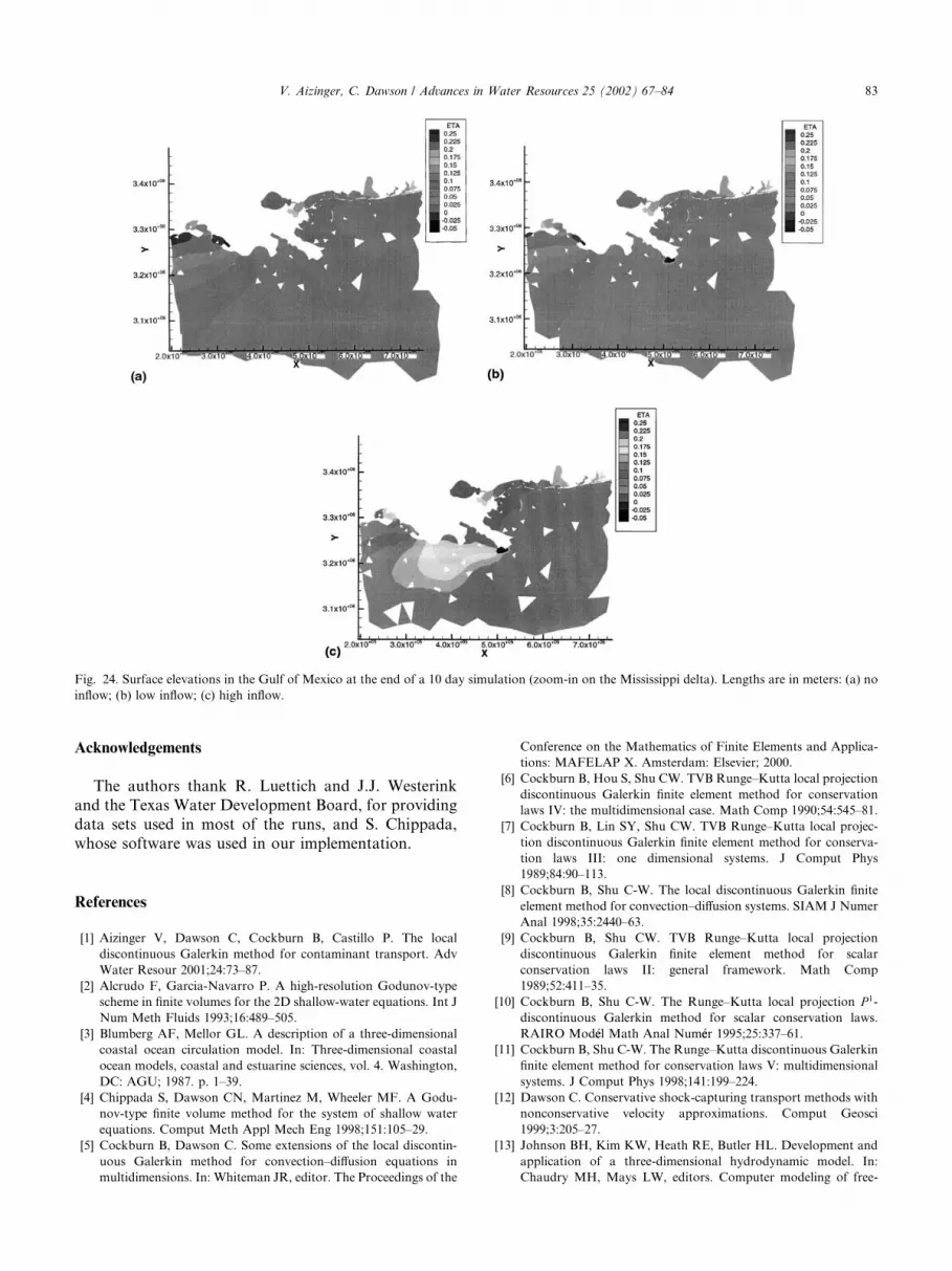
Our final scenario is a study of the effects of inflowfrom the Mississippi River, which empties into the Gulfof Mexico at a point located on the southeasternLouisiana coast, on water elevation in the Gulf. Thefinite element mesh and bathymetry are plotted in Fig.22. The finite element mesh consists of 14269 elementsand is highly graded near the US coast. An open-seaboundary condition is imposed similar to that givenabove for the previous two test cases. Three cases areconsidered: no inflow, low inflow (5000 m3 s�1) andhigh inflow (35000 m3 s�1). Piecewise constant approx-imations were used in these simulations and the timestep was set to 5 s.Surface elevations at the end of a 10 day simulation for

the three cases are plotted in Figs. 23(a)–(c). Figs. 24(a)–(c) zoom inon theMississippi delta to give a better viewofthe local distribution of surface elevation. As seen in thefigures, the water elevation changes very slightly and onlynear the mouth of the river when comparing no inflow(Figs. 23(a) and 24(a)) to low inflow (Figs. 23(b) and24(b)), indicating that for ‘‘normal’’ flow conditions, theriver does not greatly effect surface elevations in the Gulf.For the high inflow case (Figs. 23(c) and 24(c)) however,elevation increases approximately half-a-foot along thelower Louisiana coast, indicating what might occur dur-ing this type of ‘‘flood’’ situation.

Fig. 17. Absolute (a) and relative (b) error of mass conservation.


6. Conclusions

In this paper, we have described a discontinuousGalerkin finite element method for approximatingshallow-water hydrodynamics and contaminant trans-port. The method has been applied to some super-critical flow test cases and to some typical flowproblems, including tidal flows in Galveston Bay and

river inflow in the Gulf of Mexico. The method sup-ports both lower-order and higher-order approxima-tions, and locally conserves both mass andmomentum. The numerical results obtained so farindicate that for the test problems considered, themethod is capable of approximating sharp fronts in-duced by high speed flows as well as smooth flowsinduced by tidal boundary conditions. Furthermore,

Fig. 18. Comparison of linear (solid line) and constant (+) x-velocity approximations at Galveston Bay locations 1–3 for t ¼ 9–12 days.


Fig. 19. Comparison of linear (a) and constant (b) velocity approximations U in Galveston Bay at the end of day 11.

Fig. 20. Comparison of linear (a) and constant (b) velocity approximations V in Galveston Bay at the end of day 11.

Fig. 21. Comparison of linear (a) and constant (b) elevation approximations n in Galveston Bay at the end of day 11.


while piecewise constant approximations can capturethe qualitative dynamics of the flow in most cases,piecewise linear approximations do a better job ofresolving sharp variations in the solutions.

Future work includes extending the DG methodol-ogy to three-dimensional baroclinic hydrodynamics,and incorporating h (mesh) and p (polynomial order)adaptivity into our simulator.

Fig. 23. Surface elevations in the Gulf of Mexico at the end of a 10 day simulation. Lengths are in meters: (a) no inflow; (b) low inflow; (c) high

inflow.

X

Y

0.0x10+00 5.0x10+05 1.0x10+062.0x10+06

2.5x10+06

3.0x10+06

3.5x10+06

Louisiana

Mississippi

land

land

open sealand

open sea

X

Y

0.0x10+00 5.0x10+05 1.0x10+062.0x10+06

2.5x10+06

3.0x10+06

3.5x10+06 DP36003400320030002800260024002200200018001600140012001000800600400200

(a) (b)

Fig. 22. Gulf of Mexico mesh (a) and bathymetry (b). Lengths are in meters.


Acknowledgements

The authors thank R. Luettich and J.J. Westerinkand the Texas Water Development Board, for providingdata sets used in most of the runs, and S. Chippada,whose software was used in our implementation.

References

[1] Aizinger V, Dawson C, Cockburn B, Castillo P. The local

discontinuous Galerkin method for contaminant transport. Adv

Water Resour 2001;24:73–87.

[2] Alcrudo F, Garcia-Navarro P. A high-resolution Godunov-type

scheme in finite volumes for the 2D shallow-water equations. Int J

Num Meth Fluids 1993;16:489–505.

[3] Blumberg AF, Mellor GL. A description of a three-dimensional

coastal ocean circulation model. In: Three-dimensional coastal

ocean models, coastal and estuarine sciences, vol. 4. Washington,

DC: AGU; 1987. p. 1–39.

[4] Chippada S, Dawson CN, Martinez M, Wheeler MF. A Godu-

nov-type finite volume method for the system of shallow water

equations. Comput Meth Appl Mech Eng 1998;151:105–29.

[5] Cockburn B, Dawson C. Some extensions of the local discontin-

uous Galerkin method for convection–diffusion equations in

multidimensions. In: Whiteman JR, editor. The Proceedings of the

Conference on the Mathematics of Finite Elements and Applica-

tions: MAFELAP X. Amsterdam: Elsevier; 2000.

[6] Cockburn B, Hou S, Shu CW. TVB Runge–Kutta local projection

discontinuous Galerkin finite element method for conservation

laws IV: the multidimensional case. Math Comp 1990;54:545–81.

[7] Cockburn B, Lin SY, Shu CW. TVB Runge–Kutta local projec-

tion discontinuous Galerkin finite element method for conserva-

tion laws III: one dimensional systems. J Comput Phys

1989;84:90–113.

[8] Cockburn B, Shu C-W. The local discontinuous Galerkin finite

element method for convection–diffusion systems. SIAM J Numer

Anal 1998;35:2440–63.

[9] Cockburn B, Shu CW. TVB Runge–Kutta local projection

discontinuous Galerkin finite element method for scalar

conservation laws II: general framework. Math Comp

1989;52:411–35.

[10] Cockburn B, Shu C-W. The Runge–Kutta local projection P 1-discontinuous Galerkin method for scalar conservation laws.

RAIRO Mod�eel Math Anal Num�eer 1995;25:337–61.[11] Cockburn B, Shu C-W. The Runge–Kutta discontinuous Galerkin

finite element method for conservation laws V: multidimensional

systems. J Comput Phys 1998;141:199–224.

[12] Dawson C. Conservative shock-capturing transport methods with

nonconservative velocity approximations. Comput Geosci

1999;3:205–27.

[13] Johnson BH, Kim KW, Heath RE, Butler HL. Development and

application of a three-dimensional hydrodynamic model. In:

Chaudry MH, Mays LW, editors. Computer modeling of free-

Fig. 24. Surface elevations in the Gulf of Mexico at the end of a 10 day simulation (zoom-in on the Mississippi delta). Lengths are in meters: (a) no

inflow; (b) low inflow; (c) high inflow.


surface and pressurized flows. Dordrecht: Kluwer Academic

Publishers; 1994. p. 241–80.

[14] Ippen AT. Mechanics of supercritical flow. Trans ASCE 1951;

116:268–95.

[15] Kawahara M, Hirano H, Tsuhora K, Iwagaki K. Selective

lumping finite element method for shallow water equations. Int J

Num Meth Eng 1982;2:99–112.

[16] King IP, Norton WR. Recent application of RMA’s finite element

models for two-dimensional hydrodynamics and water quality. In:

Brebbia CA, Gray WG, Pinder GF, editors. Finite elements in

water resources II. London: Pentech Press; 1978.

[17] Luettich RA, Westerink JJ, Scheffner NW. ADCIRC: an ad-

vanced three-dimensional circulation model for shelves, coasts

and estuaries, report 1. Washington, DC, 20314-1000: US Army

Corps of Engineers. December 1991.

[18] Lynch DR, Gray W. A wave equation model for finite element

tidal computations. Comput Fluids 1979;7:207–28.

[19] Roe PL. Approximate Riemann solvers, parameter vectors, and

difference schemes. J Comput Phys 1981;43:357–72.

[20] Szymkiewicz R. Oscillation-free solution of shallow water equa-

tions for nonstaggered grid. J Hydraul Eng 1993;119:1118–37.

[21] Vreugdenhil CB. Numerical methods for shallow-water flow.

Dordrecht: Kluwer Academic Publishers; 1994.

[22] Weiyan T. Shallow-water hydrodynamics. Elsevier Oceanography

Series, vol. 55. Amsterdam: Elsevier; 1992.

[23] Zienkiewicz OC, Ortiz P. A split-characteristic based finite

element model for the shallow water equations. Int J Num Meth

Fluids 1995;20:1061–80.


A discontinuous Galerkin method for two-dimensional flow and transport in shallow water

Documents

Transcript of A discontinuous Galerkin method for two-dimensional flow and transport in shallow water