A detailed study of equatorial electrojet phenomenon using

Ørsted satellite observations

Geeta Jadhav, Mita Rajaram, and R. RajaramIndian Institute of Geomagnetism, Mumbai, India

Received 21 June 2001; revised 30 November 2001; accepted 10 December 2001; published 10 August 2002.

[1] Detailed analysis of the scalar magnetic field data from Ørsted satellite for quiet daysfrom April 1999 to March 2000 has been undertaken to study the equatorial electrojet(EEJ) phenomenon. An objective technique has been adopted for the identification of theEEJ from the satellite data and estimation of the standard parameters associated with it.EEJ strength computed using the satellite data and simultaneous ground magneticobservatory data, for the Indian and American sectors, correlate very well authenticatingthe method used. Estimated zonal variation in the EEJ parameters such as peak currentintensity (J0), and total current (I+) are broadly consistent with the earlier observations.We, however, observe that the width of the EEJ varies considerably with longitude, afeature not seen in the Pogo data. The study shows that the EEJ axis (center of EEJ)closely follows the dip equator at altitude of 106 km, but there is a small departure thatundergoes diurnal variation, with a minimum at noon. The globally averaged EEJamplitude follows the expected diurnal pattern. Principal component analysis techniquereveals that first four components can explain around two thirds of the electrojetvariability. The first component, which contributes a little over 30% to the observedvariance, could be identified with the global variation of the EEJ emanating from the day-to-day variability of the migrating tides. The second and fourth components, whichaccount for around 15 and 10% of the variance, respectively, are driven by forcing thatdepends on whether the location of the EEJ in that sector is in the Northern or SouthernHemisphere. The third component provides maximum contributions wherever thegeomagnetic and dip equators are sufficiently close, accounting for 12.5% of the variance.The remaining components could be associated with contribution of nonmigratory tides orother unknown mechanisms. Thus the present study suggests that besides conductivity,atmospheric tidal modes play important role in defining the zonal variability of the EEJcurrent system. INDEX TERMS: 2409 Ionosphere: Current systems (2708); 2415 Ionosphere: Equatorial

ionosphere; KEYWORDS: equatorial electrojet, satellite magnetic measurements, principal component analysis,

longitudinal variation

1. Introduction

[2] The equatorial electrojet (EEJ) represents an enhance-ment of the diurnal variation in the geomagnetic field nearthe dip equator. Extensive studies of the EEJ have beencarried out for many years using ground observations[Rastogi, 1989]. Study of EEJ phenomenon using satellite[Cain and Sweeney, 1973] has a distinct advantage that itcan provide true global coverage. Following Cain andSweeney [1973], a number of investigations have beencarried out using the Pogo data [cf. Onwumechili, 1997,and references therein], which have shown that the longi-tudinal variation of EEJ strength cannot be accounted for bythe longitudinal changes in the Cowling conductivity. Iden-tification of meridional currents associated with the EEJbecame possible with Magsat vector magnetic data [Maedaet al., 1982; Langel et al., 1993].

[3] In the present communication we have reported theresults obtained from a statistical study of the scalarmagnetic field data of Ørsted satellite. The EEJ can beclearly identified on almost all the passes of the Ørsted data[Jadhav et al., 2002]. The local time and altitude of thesatellite for the passes during the day varies very little, and itis possible to get the electrojet strength at different longitudezones on the same day. The Ørsted satellite thus constitutesa very valuable set of data for studies of the EEJ. In ourearlier study [Jadhav et al., 2002], we had looked into theextent of geomagnetic main field control over the EEJ.Here, we make a more quantitative estimate of the EEJparameters and its day-to-day variability as seen in thesatellite data.[4] In section 2, Ørsted data are briefly introduced, and

the preliminary treatment required for isolating the EEJsignature is laid out. In section 3, we discuss the basicmodel used for the EEJ analysis, method of analysis, anddifferent EEJ parameters that are obtained in present study.In section 4, the validation of identified parameters through

JOURNAL OF GEOPHYSICAL RESEARCH, VOL. 107, NO. A8, 1175, 10.1029/2001JA000183, 2002

Copyright 2002 by the American Geophysical Union.0148-0227/02/2001JA000183

SIA 12 - 1

Correction published 28 February 2004

comparison with ground magnetic observations is dis-cussed. In section 5, the statistical relationship, betweenthe derived EEJ parameters, are discussed in detail. Section6 examines the longitudinal and local time variation of EEJ,while in section 7, we look at the problem of the variabilityof the EEJ from day to day. Results and discussion havebeen accommodated in section 8.

2. Preliminary Treatment of the Ørsted Data

[5] The polar orbiting Danish Meteorological Institute(DMI) satellite Ørsted was launched on 23 February 1999[Neubert et al., 2001]. In the present analysis we use scalarmagnetic field measurements recorded by the Overhauserproton magnetometer, on board the satellite. The data havean absolute accuracy better than 0.3 nT. The orbital periodis �100 min; that leads to �15 day and an equal numberof night passes. The longitude and local time (LT) incre-ment is �25� per orbit and �0.88 min per day, respec-tively. Hence, for a given date, all the daytime passes havealmost the same local time. In this paper, we have analyzed12 months of scalar magnetic field data from April 1999to March 2000 with LT varying from 13.6 to 9.5 hours.Table 1 gives the typical local times of the passes frommonth to month.[6] The signature of the EEJ becomes weaker as the

height of the satellite orbit increases. As disturbances ofmagnetospheric origin can mask the typical signature of theEEJ at the orbit of Ørsted, the analysis has been restricted togeomagnetic quiet days. Only the data from the 5 Interna-tional Quiet Days (IQ) of each month is used in the analysis.This does not grant immunity against intrusions of magneticdisturbance effects considering the fact that we are close tothe solar maximum and few days are entirely free ofgeomagnetic disturbances. The main field is removed usingIGRF 2000, supplied by Ørsted team [Olsen et al., 2000].The basic inputs for the main field computation are thesatellite location and the hourly Dst values which are readilyavailable at the World Data Centers (WDCs).[7] The residual magnetic field �F includes fields pro-

duced by external current sources like the EEJ, Sq, andmagnetospheric currents. This is subjected to low passfiltering using 203-point sine-terminated low pass filter withleast squares approximated transfer functions [Behannon

and Ness, 1966] to remove spatial wavelength less than 4�,before it is used to identify the EEJ. A typical EEJ signaturein the satellite profile has been clearly described by Cainand Sweeney [1973]. The expected latitudinal profile isshown in Figure 1. The signature is characterized by aminimum at the latitude of the EEJ axis accompanied by‘‘shoulders’’ of increased field on either side. Verticaldistance between dip and shoulders (CC’) in Figure 1, is ameasure of the strength S of the contribution of EEJ currentsat the satellite location and the horizontal distance betweentwo shoulders (WW’) gives the width of signature atsatellite height of the EEJ current system. The Pogo andMagsat satellite studies successfully used this typical sig-nature for identifying the EEJ. It is therefore adopted in theanalysis of the Ørsted data.[8] A Fortran program was developed to automatically

identify EEJ signatures from the selected satellite orbitaldata restricted to ±20� dip latitude and to process and storethe transformed data useful for evaluation of the EEJparameters. Out of 839 passes, only those that showed awell-defined minimum within ±5� of the dip equator wereconsidered. The program takes care of the following alter-natives:1. The minimum is accompanied by two maximum

values, one on either side; those positions of maxima definethe edges of the EEJ.2. The second maximum is only registered as a change in

gradient; this is considered as the second edge.3. Only one maximum is identified; a point symmetri-

cally located on the other side of the minimum is taken asthe position of the second edge.4. Neither of the two maxima is discernible; in this case

edges are assumed to be located at ±12�.[9] A linear trend is removed to bring the two edges to

the same level. In case of 2, 3, and 4 a cubic fit to our low-latitude data segment outside the EEJ belt (defined by twoedges of EEJ) is removed. These two steps are repeated(maximum of 5 times) in attempt to get the ideal situationdefined in case 1.

Table 1. Local Times of the Passes in Different Months

Month LT, hour

1999April 13.6May 13June 12.7July 12.5August 12September 11.5October 11November 10.5December 10

2000January 9.5February 9March 8.5

Figure 1. Typical signature of the latitudinal profile of theresidual field observed at Ørsted satellite height for 135�Elongitude pass, on 2 August 1999.

SIA 12 - 2 JADHAV ET AL.: TECHNIQUES

[10] The entire �F profile for each of the passes, con-sisting of around 300 to 350 data points, is used forobtaining the EEJ parameters. The 513 ideal EEJ signaturepasses as well as the 267 passes for which the signature wasclear in one hemisphere and suggestive (but not so explicit)in the other hemisphere are used for the statistical study ofestimates of the EEJ parameters. It should be mentioned inpassing here that 45 of the satellite �F profiles had distinctreversed EEJ signature. Data from these passes are not usedin this analysis.

3. Determination of EEJ Parameters

[11] We shall take the point of view that the typicalsignature at satellite altitude above EEJ current systemshown in Figure 1 is associated with an eastward currentflowing near dip equator and westward current on bothflanks of the magnetic dip equator. We use the model forEEJ due to Onwumechili [1997, p. 145], which can repro-duce the dip as well as the shoulders seen in the satellite.The northward, X and vertical, Z components of the mag-netic field from the continuous distribution of currentdensity model

J ¼ J0a2 þ a:x2ð Þa2 þ x2ð Þ2

b2

b2 þ z2ð Þ2

is given by [Onwumechili, 1997, p. 279]

sg � zð ÞP4X ¼ 1

2Ka vþ avþ 2aað Þ uþ bð Þ2

hþ vþ avþ 2að Þ vþ að Þ2

ið1Þ

� sg:xð ÞP4Z ¼ 1

2Ka uþ bð Þ 1þ að Þ uþ bð Þ2

hþ vþ avþ 3a� aað Þ vþ að Þ

i; ð2Þ

where P2 ¼ uþ bð Þ2þ vþ að Þ2, K = 0.2pJ0,

u ¼ xj j; v ¼ zj j; sg � x ¼ sign of x ¼ x

u; sg � z ¼ sign of z ¼ z

v:

[12] Here, the center of the current system has beentaken as the origin, x is the latitudinal distance measurednorthward from the origin, y is eastward, and z is verticallydownward distance from the current layer. The a and bvalues are latitudinal and vertical scale lengths, respec-tively, a is dimensionless constant controlling latitudinaldistribution of current, J0 is the peak current intensity orthe height-integrated current density at the center of thecurrent system. If X and Z are in nanoteslas, then J0 is inAmperes/km.[13] The identification of the EEJ parameters is based on

the above empirical model. Many of the earlier studies [e.g.,Onwumechili, 1997 p. 296] had used the same model, butthey based their estimations on the magnitude S (defined insection 2) and did not make use of the full EEJ signature atthe satellite location. In order to derive the parameters K, a,and a they assume that given the longitude and local time,these parameters do not vary from day to day. Using

different sets of (S, h), where S is the EEJ strength at EEJaxis at altitude h of the satellite, they solved the aboveequations to get K, a, and a. However, we find that theshape of the signature (i.e., width and strength) changesfrom day to day even at a given longitude and LT. Hence wehave computed parameters K, a, and a for each pass using300 to 350 data points defining the structure identified andstored by the process described in section 2.[14] For the estimation of the EEJ parameters we have

assumed that the EEJ current flows at a height of 106 km inthe ionosphere and neglected the subsurface induced cur-rents for computing the field at the satellite height. There issome justification in making such assumptions. A numberof rocket measurements in the equatorial region haveconfirmed that the peak electrojet current flows at 106-kmaltitude [Sampath and Sastry, 1979]. Fambitakoye andMayaud [1976] found no measurable induction of theelectrojet field in Central Africa, while Ducruix et al.[1977] have shown theoretically that electrojet-induced fieldis negligible at least along the noon meridian. Yacob [1977]examined internal induction by the EEJ in India withground and Pogo satellite geomagnetic observations andfound that its internal field contribution is small. This couldbe regarded as some justification for neglecting geomag-netic induction. Furthermore, subsurface conductivity isalso a variable quantity and making even intelligent guessesof its underlying longitudinal structure would lead to a biasin the estimated induced currents.[15] The scalar field �F ¼

ffiffiffiffiffiffiffiffiffiffiffiffiffiffiffiffiffiX 2 þ Z2

p� �is computed

using equations (1) and (2). For each EEJ pass, parametersa and a are varied iteratively until they produce shoulders atright locations. The parameter K is obtained through leastsquares fit to �F along the satellite profile that incorporatesa constant background shift. The best fit is decided by thecross correlation between the observed and computed pro-files as well as the mean square differences between them.The parameter set with lowest mean square difference and across correlation greater than 0.7 is selected. The method-ology is fully automated and objective. However, it has tobe tested with independent data to establish its authenticityand statistical reliability. This is achieved in section 4through the comparison of H (the horizontal componentof the magnetic field) of the observatory magnetic field datawith the H variation on ground computed using overheadsatellite measurements.

4. Comparison Between Satellite and GroundObservations

[16] For comparisons, we use observatory data with diplatitude l, geographic longitude f, from Trivandrum (l =0.43�, f = 76.9�E) and Alibag (l = 13.06�, f = 72.9�E) inthe Indian sector and Huancayo (l = 0.59�, f = 284.7�E)and Fuquene (l = 17.11�, f = 286.3�E) in the Americansector. The comparison with ground data was made frompass to pass. Identification of the EEJ on ground requires atleast two stations, one close to the dip equator (the electrojetstation) and the other a low-latitude station (nonelectrojetstation) just outside the influence of the EEJ [Bhargava andYacob, 1973]. Comparisons were possible only when thesatellite passed within longitude range of ±5� of the longi-tude of the stations or when there were at least two passes in

JADHAV ET AL.: TECHNIQUES SIA 12 - 3

a day within longitude range of ±30� of the longitude of thechosen stations. In the first case the field on ground wascalculated using the parameters determined for the givenpass. In the second case the field computed at the twolongitudes corresponding to the satellite passes were inter-polated to obtain the field in the longitude zone of the givenchosen stations. In doing so, it has been tacitly assumed thatthe EEJ field has the same local time (LT) pattern atneighboring longitudes and the two values around 100min apart can still be used for interpolating in longitudeto get EEJ field at the given longitude and LT. Equation (1)is used to obtain the EEJ contribution to H at any latitude.[17] For estimating the EEJ field on ground in the Indian

sector, hourly values of Trivandrum and Alibag magneticobservatories were used. Nighttime means were subtractedfrom the daytime hourly values, and these were interpolatedto determine the H at the local time of the crossing of theØrsted satellite. The interpolated value for Alibag wassubtracted from that at Trivandrum to obtain the instanta-neous value of EEJHobs at the time of satellite overheadcrossing. Similar data reduction techniques were utilized forFuquene, but in the case of Huancayo, the daily traces hadto be down loaded from WDC, Kyoto site and redigitized.[18] The estimate of the electrojet strength on ground

from the satellite parameters is obtained by computing the Hat the axis of the EEJ current system as deduced from thesatellite data. The correlations between EEJHobs (theobserved electrojet strength on ground) and EEJHcomputed

(the estimated strength based on the satellite data) arepresented separately for American (Figure 2) and Indian(Figure 3) sectors. The scatter is symmetrically distributedabout the mean regression line, and the correlation coef-ficient is 0.86 in both Indian and American sectors. Thiscompares favorably with the results of Yacob [1977], whofound correlation coefficient of around 0.88 between thesurface electrojet strength observed in the Indian region,extrapolated to the satellite height using a parabolic current-band model of electrojet, and the strength as obtained from

satellite measurements. These correlations for the givennumber of points are significant at 99.9% level. Theexcellent match confirms that the algorithm used hasprovided reliable estimates of a and K and fully authenticatethe technique used for deducing the EEJ parameters fromthe satellite data. Subsurface currents are expected to addto the surface H, and the slope of regression line is probablygreater than unity because of the neglect of the inductioneffect. We do not claim a perfect estimation from pass topass, but it can be justifiably argued that the estimationsshould provide the basis for the investigations of thestatistical properties of the EEJ in different longituderegions around the globe.

5. Statistical Relationship Between EEJParameters

[19] There are four main parameters of the EEJ whoselongitudinal variations have been discussed in literature[Onwumechili, 1997]. These are the peak of the EEJcurrent given by Jo, the position of the electrojet axis xo,the estimated width of the EEJ given by W ¼ 2a=

ffiffiffiffiffiffiffi�a

p

and I+, the total amount of positive eastward current inamperes flowing between the two locations of zero inten-sity given by

Iþ ¼ aJo �að Þ1=2þ 1þ að Þ tan�1 1

�a

� �1=2" #

: ð3Þ

[20] In discussion, we also mention the width of EEJ atsatellite and ground. The width of EEJ at satellite (Wsatellite)is the direct observation of the distance between two peaksin the EEJ signature at satellite altitude and that on ground(Wground) is the distance between two minima in the EEJsignature computed on ground from the model parameters.The overall nature of the parameters derived from thesatellite data is depicted in Figures 4a–4e. There is a clearpositive correlation between Jo, the peak current density andHaxis, the computed field at the EEJ axis on ground(Figure 4a). The scatter about the fitted straight line may

Figure 2. Scatterplot of equatorial electrojet (EEJ) Hobs

from American observatory data plotted against the EEJHcomputed computed at the axis of EEJ from satellite basedEEJ parameters.

Figure 3. Same as Figure 2, for Indian region.

SIA 12 - 4 JADHAV ET AL.: TECHNIQUES

be mainly attributed to variability in a. This scatter is not anindication of errors but only emphasizes the fact that thesurface field is not entirely determined by the peak currentdensity. This is brought out by the reduced scatter in thestraight-line fit when I+ is used instead of Jo (Figure 4b).This reduction in scatter shows that I+ and not Jo is morerelevant as far as ground magnetic effects are concerned.[21] The relationship between Wground, and the width W at

the position of current system (Figure 4c) is linear, but thereis also a scatter that underlines the fact that two independentparameters a and a together determine the relationshipbetween the width of EEJ at ground and 106 km, whichis therefore not simple and straightforward. The relationshipbetween Wsatellite and Wground that is not plotted here is alsolinear, but the width at the satellite height is �3 times thewidth on ground.[22] Relationship between Jo and the width of the EEJ

(W ) at 106 km is plotted in Figure 4d, which suggests thatlarger values of the peak current density are associated withsmaller scatter in the width of the latitudinal structure of theelectrojet. This scatter may probably imply that when Jo issmall the signature of the EEJ at the satellite heights aresmaller, and hence there is a greater chance of errorscreeping in derivation of the structural parameters a anda, which ultimately determine the width of the EEJ. Thespread could also arise owing to the fact that smaller peakcurrents may require larger width to reproduce a givensignature at the satellite height. The standard deviations ofthe spread of the width scatter are reasonable, and theparameter can thus supply reliable statistical data on theEEJ. Finally, Figure 4e shows how the position of axis ofthe electrojet current system (with respect to the dipequator) controls the electrojet strength on ground. The

diagram clearly demonstrates the fact that strength of EEJis considerably reduced when its axis shifts away fromthe dip equator. The results can be expected on physicalgrounds.[23] In conclusion, Figures 4a–4e suggest that the param-

eters determined from the Ørsted passes are suitable for thestudy of the statistical properties of the EEJ, though it maynot be the right choice for detailed analysis of individual casestudies. In what follows, we concentrate on the statisticallyaveraged values of the derived EEJ parameters and examinetheir dependence on the longitude, season, and local time. Inthe process we shall determine whether these are consistentwith the earlier studies based on Pogo and Magsat.

6. Longitudinal and Local Time Variation ofEEJ

[24] In this section, we examine the longitudinal and localtime structure of the EEJ parameters derived from satelliteobservations. In Figure 5, we plot the longitudinal variationof average values of the current parameters I+, Jo, and W inthe ionosphere, while in Figure 6 we look at the magneticfield on the ground at the axis of the current system. Eachpoint, in these figures represents an average of all the passesin a 30� bin centered at longitudes 5�, 15�, 25�, etc. In theseplots, as well in all the plots that follow, the error barcorresponds to the estimated standard error of the mean.[25] The peaks in the total eastward current I+ (Figure 5a)

are in broad agreement with those determined for the Pogosatellite data byOnwumechili and Agu [1981]. Note also thatthe longitudinal variation of the EEJ strength on ground(Figure 6, left topmost) is almost identical to that of I+ but notto J0. Onwumechili and Agu [1981] get three well-defined

Figure 4. Scatterplot for EEJ parameters determined from satellite data. See text for definition ofparameters.

JADHAV ET AL.: TECHNIQUES SIA 12 - 5

peaks for J0 centered at 100�, 190�, and 270�E and a smallerpeak around 350�E. We do not get the peak at 270�E.

Furthermore, the magnitudes of the peaks are less in ourcase, and two less clearly defined peaks at 70� and 120�replace the peak at 100� obtained by them. The dusk timehorizontal currents deduced from Magsat analysis [Langel etal., 1993] revealed peaks at 280�E and between 110� and150�E but showed no clear peak around 100�E. However,some of their figures depicting eastward electrojet signaturesdo show indications of peak at 360�E and around 180�E.[26] Figure 5c shows that the width of the EEJ current

system is largest in the American sector, and this is respon-sible for the strong peak in the EEJ strength at 270�E,though it is not reflected in J0. Larger width of the currentsystem will be associated with larger a, and it is not difficultto see from equations (1) and (2) that this will lead to largermagnetic field on ground. There are also two secondarypeaks at 30� and 105�E longitudes. The peaks are welldefined and statistically significant. The width varies from2.5� in the region 150�E to as much as 6.5� in the Americanzone. Though the width of 4� obtained for the Indian zone isfairly consistent with the halfwidth of 2.9� reported by Okoet al. [1996] using observatory data, the variation of thewidth of EEJ current system with longitude is much greaterthan that reported by Onwumechili and Agu [1981].[27] A simple theoretical explanation based on increased

ionospheric conductivity [Cain and Sweeney, 1973] cannotexplain this multipeak structure (Figure 6, left topmost), and

this may have to be attributed to tidal variability. It should benoted that we are discussing longitudinal structures averagedover a range of seasons/LT, and thus many of the seasonaland LT influences remain hidden. Some of these are reflectedin the remaining plots of Figure 6. Plots on the left-hand sideshow average amplitude of electrojet strength on ground fordifferent months labeled as March (February–March 2000,0820–0910 LT), June (May–July 1999, 1210–1320 LT),September (August–October 1999, 1040–1200 LT) andDecember (November 1999 to January 2000, 0920 to 1040LT). The right-hand side plots show amplitude averages fordifferent local times labeled as 0830 to 0930 (17 January to27 March 2000), 0930 to 1030 (30 November 1999 to 9January 2000), 1030 to 1130 (8 September to 15 November1999), 1130 to 1230 (4 July to 6 September 1999) and 1230to 1330 (25 April to 30 June 1999).[28] The peak around 0�E is persistent right through

while the peak around 270�E remains from June to Sep-tember. The peak around 110�E is most clearly seen fromMarch to June. At 1100 LT, peak at 110� splits into two; oneappears at 90� and the other at 125�. Around 180�–200�E,where the geographic and geomagnetic equators are coin-cident, the peak is very distinct only from December toMarch. The LT plot shows that the peaks in this sector arelargest between 0830 and 0930 LT, where it is comparablewith that of the other peaks at 1100 LT. As LT increases, itsstrength decreases while the peaks at other longitudes startbuilding up. We examined the data at Jarvis Island (l =1.11�; f = 199.97�E) and did not find any unusual LT traitsthat could justify such an early LT peak in EEJ. This

Figure 6. The longitudinal variation of the computedstrength of the EEJ (nanoteslas) on ground at the position ofthe axis. The top plot shows the average pattern, the bottomleft depicts the variations categorized in to different months,while the bottom right shows the variation categorized interms of the local time of the satellite pass.

Figure 5. Longitudinal structure of (a) I+, (b) J0, and(c) the electrojet width W plotted as a function of longitude.Error bars are estimated variance of the mean.

SIA 12 - 6 JADHAV ET AL.: TECHNIQUES

suggests that we are looking at a seasonal effect, and thisparticular peak would probably have been much larger if thesatellite pass had been around noon in December to Marchsector. Similarly, the fact that the field at 270�E is found tobe largest between 1230 and 1330 LT may also be attributedto a seasonal effect. Baring a couple of these sectors,elsewhere the peaks at 1030 to 1130 LT dominate indicatingthat the LT dependence that is probably most apparent. Thiscan be seen in the mean picture presented next.[29] We have already noted from Figure 4e that the EEJ

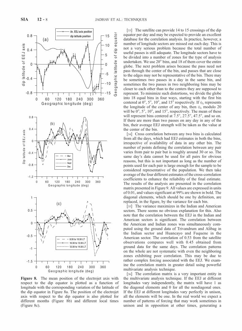
strength on ground decreases as its axis moves substantiallyaway from the dip equator. This is further substantiated bythe results presented in Figures 7a and 7b. In Figure 7a wehave shown the variation of the mean field on ground at theaxis of EEJ current system, as a function of the local time ofthe pass. While in Figure 7b we depict the mean of themagnitude of the deviation of the position of the axis ofthe EEJ current system with respect to the dip equator. Themean is taken over data from all the longitude zones. Theelectrojet strength on ground shows the expected temporalvariation peaking around 1130 LT and decreasing on eitherside. The position of the EEJ current axis also shows asystematic temporal pattern being closest to the dip equatoraround the time when the H on ground maximizes. Thisis consistent with the scatterplot depicted in Figure 4e,but more importantly, it corroborates the findings ofFambitakoye and Mayaud [1976], who also found that theEEJ current axis is located closest to the dip equatornear local noon. This definitely adds credibility to thealgorithms used here.[30] We next look (Figure 8a) at the magnitude of the

shift of the axis of EEJ current system from the dip equatoras a function of longitude averaging over all LT (or months).Note that with the exception of regions close to 150�E, theEEJ current axis shifts away from the dip equator toward thegeographic equator. These results are consistent with thoseof Cain and Sweeney [1973]. This feature is fairly persistentwhether data is classified by month (Figure 8b) or by LT(Figure 8c). In the longitude regions near 30�E, 285�E and315�E, the deviation of EEJ axis from the dip equator issystematically larger (>0.5�). The plots appear less system-atic when classified according to season than according toLT. This adds credence to the argument, that the movementof the position of center of EEJ system depicted in

Figure 8c, represent genuine LT variations adding strengthto the conclusions arrived at in the last section.

7. Day-to-Day Variability in Surface MagneticField

[31] What we have examined so far is the average pattern.Of much greater relevance is the variability from day to day.There is a longitudinal dependence of the EEJ strengthbecause the Cowling conductivity that is responsible for theelectrojet has a longitudinal dependence [Cain and Swee-ney, 1973; Jadhav et al., 2002]. The next question that oneasks is whether the EEJ strength strictly follows the longi-tudinal structure defined by the conductivity every day. Wehave already seen from the average picture that the longi-tudinal structure of the EEJ is not determined entirely byconductivity. Since tides may be responsible for at leastsome of the peaks, we suspect that the day-to-day variabilitywill have a clear longitudinal structure. A recent paper byChandra et al. [2000] clearly shows that the longitudinalvariation of EEJ is not due to the variation of the con-ductivity, but due to local electric field in the ionosphere.[32] James et al. [1996] studied the day-to-day variability

using latitudinal array of stations in a narrow range oflongitude and found that the correlation of �H at anystation with equatorial station decreases as latitude of thestation increases. Rangarajan [1992] using method of linearpredictor filters have examined the relation between EEJvariations, at two ground stations separated in longitude. Hewas able to demonstrate that the electrojet H at Addis Ababacould be predicted fairly efficiently, given the time series ofTrivandrum. The method is not easily applicable withsatellite database of the type we have. Schlapp [1968]studied the variability of the EEJ from one day to anotherusing coefficient of cross correlations between ground geo-magnetic stations. He found that correlation drops to lessthan 0.5, if two stations are separated by 40� in longitude.We propose to use a similar cross-correlation technique withthe satellite data. The satellite data cover areas of the globenot accessible to surface measurements and can be expectedto provide a more complete information. Right throughthis section EEJ strength represents the magnitude of theelectrojet on ground calculated using parameters derivedfrom satellite observations.

Figure 7. (a) The mean electrojet strength H on ground and (b) the shift of the latitude of the axis of theEEJ from the dip equator are plotted as a function of local time.

JADHAV ET AL.: TECHNIQUES SIA 12 - 7

[33] The satellite can provide 14 to 15 crossings of the dipequator per day and may be expected to provide an excellentdatabase for the correlation analysis. In practice, however, anumber of longitude sectors are missed out each day. This isnot a very serious problem because the total number ofuseful passes is still adequate. The longitude sectors have tobe divided into a number of zones for the type of analysisundertaken. We use 20� bins, and 18 of them cover the entireglobe. The next problem arises because the pass need notpass through the center of the bin, and passes that are closeto the edges may not be representative of the bin. There maybe sometimes two passes in a day in the same bin, andsometimes the two passes in two neighboring bins may becloser to each other than to the centers they are supposed torepresent. To minimize such distortions, we divide the globeinto 18 equal bins in four ways, starting with the first bincentered at 0�, 5�, 10�, and 15� respectively. If fc representsthe longitude of the center of any bin, then fc modulo 20will be 0�, 5�, 10�, and 15�, respectively. The mean of thesewill represent bins centered at 7.5�, 27.5�, 47.5�, and so on.If there are more than two passes on any day in any of thebin, their average EEJ strength will be taken as the value atthe center of the bin.[34] Cross correlation between any two bins is calculated

from all the days, which had EEJ estimates in both the bins,irrespective of availability of data in any other bin. Thenumber of points defining the correlation between any pairvaries from pair to pair but is roughly around 30 or so. Thesame day’s data cannot be used for all pairs for obviousreasons, but this is not important as long as the number ofpoints used for each pair is large enough for the sample to beconsidered representative of the population. We then takeaverage of the four different estimates of the cross-correlationcoefficients to enhance the reliability of the final estimate.The results of the analysis are presented in the correlationmatrix presented in Figure 9. All values are expressed in unitsof 0.01, and values significant at 99% are shown in bold. Thediagonal elements, which should be one by definition, arereplaced, in the figure, by the variance for each bin.[35] The variance maximizes in the Indian and American

sectors. There seems no obvious explanation for this. Alsonote that the correlation between the EEJ in the Indian andAmerican sectors is significant. The correlation betweenthe American and Indian zones was simultaneously com-puted using the ground data of Trivandrum and Alibag inthe Indian sector and Huancayo and Fuquene in theAmerican sector. The correlation of 0.53 from the satelliteobservations compares well with 0.45 obtained fromground data for the same days. The correlation patternson the whole are not systematic with even the neighboringzones exhibiting poor correlation. This may be due torather complex forcing associated with the EEJ. We exam-ine the correlation matrix in greater detail using powerfulmultivariate analysis technique.[36] The correlation matrix is a very important entity in

the multivariate analysis technique. If the EEJ at differentlongitudes vary independently, the matrix will have 1 asthe diagonal elements and 0 for all the nondiagonal ones.If the EEJ at different longitudes vary perfectly in unison,all the elements will be one. In the real world we expect anumber of patterns of forcing that may work sometimes inunison and in opposition at other times, generating a

Figure 8. The mean position of the electrojet axis withrespect to the dip equator is plotted as a function oflongitude with the corresponding variation of the latitude ofthe dip equator in Figure 8a. The position of the electrojetaxis with respect to the dip equator is also plotted fordifferent months (Figure 8b) and different local times(Figure 8c).

SIA 12 - 8 JADHAV ET AL.: TECHNIQUES

complex correlation matrix of the type given in Figure 9.We use the principal component analysis [Gnanadesikan,1977] to determine the natural patterns of longitudinalvariations of the EEJ.[37] The basic idea of the principal component analysis is

to describe the dispersion of an n component array byintroducing a new set of coordinates so that the varianceof the given points with respect to the derived coordinatesare in decreasing order of magnitudes. In effect, instead ofrepresenting the data as values at 18 longitude points, weexpress it as coefficients of 18 orthogonal functions derivedfrom the statistical property of the data itself. The variabilityof EEJ from day to day is represented by the correspondingvariation of the coefficients of these functions. The majoradvantage of the technique is that the prescription of thechoice of the function is such that the first few functionsgenerally reproduce most of the variability in the data[Rajaram and Rajaram, 1983].[38] Let Hi,j be the EEJ value at the longitude fj ( j =

1,18) on day di (i =1, N ). We express Hi,j in the formHi; j ¼

P18k¼1

Dk dið Þ:�k fj

� �, where functions �k and Dk satisfy the

following constraints:

X18j¼1

�l fj

� �:�kðfjÞ ¼ dlk

XNi¼1

Dn dið Þ:DkðdiÞ ¼ lkdnk :

[39] The functions � and D are obtained by making a leastsquares fit to the data itself. It turns out that functions � arethe eigenvector of the matrix Rjk defined by Rjk ¼

PNi¼1

Hi; j:Hi;k andDk dið Þ ¼

P18j¼1

Hi; j:�k fj

� �. It is quite obvious that �k(fj) gives the

longitudinal structure of the kth component, and Dk(di) givesthe contribution of that particular component on day di. The

procedure is to first obtain the matrix Rik from the data anddetermine its eigenvalues and eigenfunctions. The eigenval-ues and the eigenvectors are arranged in the descendingorder. The percentage of the variance accounted for by thecomponent with eigenvalue lk is given by P ¼ ðlk=

P18j¼1

ljÞ 100:

Thus the first component explains largest percentage of thevariance, the second the next and so on.[40] We express Hi,j as departures from the mean. We

further normalize it with respect to the variance of the EEJcorresponding to that longitude bin. The matrix Ri,j thenbecomes the correlation matrix. There are distinct advan-tages in adopting this scheme. We have already noted thatEEJ strength is not obtained for all longitude bins on anygiven day. The EEJ forcing is known to be different ondifferent days, and it may be misleading to discuss thelongitudinal structure of the variability from day to day bycombining all the data together ignoring this factor. On theother hand, the correlation between any two bins is astatistic, which is reliably determined, provided the numberof common days for the two bins is large enough for thesample value to be treated as the population value. Thus it isnot necessary to restrict the analysis to days in which dataare available in all the bins selected. Consequently, bin sizescan be taken smaller to provide better resolution in longi-tude. A second advantage stems from the fact that the use ofcorrelation rather than the covariance matrix is more appro-priate for identification of coherent structures [von Storch,1999].[41] We use the correlation matrices determined earlier

for the four sets of bin distributions, which are generatedwith slight offset with respect to each other. The eigenvaluesand eigenvectors are determined and ordered in descendingvalues of their eigenvalues for each of the matrices. Each

Figure 9. Correlation matrix in units of 0.01 by zone number. Diagonal elements are the samplevariance, and the correlations significant at 99% are shown in bold face.

JADHAV ET AL.: TECHNIQUES SIA 12 - 9

normalized eigenvector has 18 elements, each of whichrepresents the contribution made at the correspondinglongitude bin. The 18th and the first bins are obviouslycontiguous. We smoothen out these contributions by takinga five-bin running mean and comparing the four differentestimates we have for the longitudinal structure of thecontributions corresponding to each of the four sets. Wefind that the first component is almost same for all the fourgroups. The same is true for the other components exceptthat the structure for the bins centered at 5� (modulo 20) isslightly different. The other three are very close to eachother, and the mean of 4 is also very close to them. Thisshows that the technique is fairly robust. Note that theoverall sign of the eigenvector is irrelevant. The contribu-tion of component is positive or negative depending uponthe sign of Dk.[42] We depict in Figure 10 the mean longitudinal struc-

ture of the first four components after multiplying contri-bution to each bin with the variance corresponding to thatbin. This multiplication with the sample variance is neces-sary to make the comparison between the different longitudezones meaningful. The percentage of the variance accountedfor each of the components is shown in Figure 11. Theresults are quite dramatic and provide considerable insightinto the different types of forcing that contributes to thevariability in the EEJ.

[43] The first component, which accounts for nearly 30%of the day-to-day variability, is obviously global in characterexcept that its contribution is slightly reduced around 240�Emeridian. It may be readily interpreted as the EEJ variabilitydue to global changes in solar ionizing radiation or migra-tory solar and lunar diurnal, semidiurnal, and higher-ordertides. The variability associated with other componentsappears to be generated by the longitudinal variations inseparation between dip and geographic equators. The geo-graphic equator orders the tidal forcing, while the dipequator dictates the symmetry of the conductivity of theionosphere. To interpret these components, we have plottedthe latitude of the dip equator along with each of thecomponents.[44] We can see that the second component, which

accounts for roughly 15% of the EEJ variability, followsthe latitude of the dip equator as function of longitudeexcept a zone between 315�E and 60�E. It is exactly in thisregion that the component four, which accounts for 10% ofthe variability, takes over and tracks the dip latitude profile.Note that the fourth component contributes in the regioneast of 330�E to the west of 30�E where the impact of thesecond component is relatively modest. These componentsproduce an equatorial EEJ contribution, which is opposite insign depending on whether the dip equator is in the North-ern or Southern Hemisphere. These could also be a sourceof the seasonal variations of the EEJ. It is not reallysurprising that two components are required to account forthe control of the latitude of the dip equator on thevariability of the strength of the observed EEJ. The regionin which the fourth component dominates corresponds tothe region where the location of the dip equator changesrapidly with longitude from around 13�S to 12�N. Thisrapid variation of the dip equator position is also accom-panied by an anomalous orientation of the dip equator withrespect to the geomagnetic field. The two are not perpen-dicular to each other as required by the classical picture ofthe equatorial EEJ. In the zone just east of 300�E longitude,the deviation from the expected perpendicularity is around12� [Jadhav et al., 2002]. We would expect that theresponse of the EEJ to changes in tidal forcing should be

Figure 10. The longitudinal structure of the first fourcomponents obtained from the principal component analysisof the satellite data is presented. Except in first component,the profile of the latitude of the dip equator (dotted line) isalso shown; the scale is shown on right-hand side.

Figure 11. Percentage of variance accounted for by thefirst four components.

SIA 12 - 10 JADHAV ET AL.: TECHNIQUES

different in such a zone and it is therefore not surprising thatan additional component manifests itself in this region.[45] Finally, component 3, which contributes around

12.5% to the EEJ variability, is most conspicuous in theregions where the dip and geographic latitudes coincide. Itis this component that contributes to the anomalously earlypeak in the 200�E region.[46] It should be pointed out that the first four compo-

nents together account for a little over two thirds of thevariability of the EEJ. The other components that areresponsible for the remaining contribution to the variabilityin EEJ could be because of various other processes includ-ing the presence of nonmigrating tides. While we havechosen only geomagnetically quiet days for our study, it isstill possible that some contribution may come from thedisturbance dynamo effects associated with the electricfields propagated from the auroral zone. The errors inherentin the determination of the EEJ parameters could also beresponsible for the apparent variability not explained by thefirst four components. We have concentrated on the longi-tudinal structure of EEJ component. No attempt has beenmade to determine Dk(di), the contribution of the kthcomponent of day di, which requires EEJ contribution ona given day from all 18 longitudinal bins.

8. Results and Discussion

[47] Using an objective method for determining theparameters of the EEJ, we have shown that magnetic fieldobservations obtained from the Ørsted satellite can form anexcellent database for studying not only the longitudinalstructure of the equatorial EEJ but also the sources respon-sible for its variations from day to day. The consistency inthe correlation of the ground observations and the corre-sponding field computed from the deduced satellite param-eters, for both the Indian and American sectors andreproduction of salient features obtained earlier [Onwume-chili, 1997] using Pogo data, is very encouraging. It should,however, be cautioned that no claim is made that theidentification of the parameters is accurate on a pass-to-pass basis. There is, however, compelling evidence to showthat the deduced parameters can reproduce statisticallyconsistent characteristics of the EEJ. Many of these featurescannot be explained on the basis of the conductivitydistribution in the equatorial ionosphere and longitude-dependent (migratory) tidal forcing has to be necessarilyinvoked.[48] By far the most far-reaching results obtained through

the analysis presented here are the conclusions based on thecorrelation analysis of the variability of the EEJ strength indifferent longitude sectors. When the correlation matricesare subjected to the principal component analysis a veryclear picture emerges. Almost two thirds of the variability inthe global variation of EEJ can be accounted for by the firstfour components taken together. The individual componentsdescribe the global as well as longitude dependence of day-to-day variability. Most significantly the importance of thegeographic latitude of the dip equator in the response of theEEJ to the day-to-day changes in the global forcing is mosteffectively brought out by the analysis. These results arefairly robust and reveal many interesting features hithertounnoticed. The technique appears to be very promising and

could find more critical application as more of the data fromthe Ørsted satellite gets analyzed.[49] It is quite remarkable that the position of the EEJ

axis deduced from satellite exhibits a local time dependencesimilar to what has been observed on ground [Fambitakoyeand Mayaud, 1976] being closest to the dip equator aroundnoon. There is also a clear indication that the EEJ strengthweakens as the axis moves away from the dip equator.These features appear in the global average, but the data setused is not large enough to make a statistically reliablestudy of the longitudinal structure of this phenomenon.[50] The distribution of the EEJ currents in longitude is

season and LT dependent and the two controlling factorscannot be separated given the limited amount of dataavailable and the season-dependent LT of the satellitepasses. The Ørsted is continuously providing data andpromises to provide the source for a more complete sta-tistics, and this deficiency will be overcome. The vectordata may also provide vital information especially withregard to the importance of meridional currents.

[51] Acknowledgments. We are grateful for support of the ØrstedProject Office and the Ørsted Science Centre at the Danish MeteorologicalInstitute. The Ørsted Project is funded by the Danish Ministry of Transport,Ministry of Research and Information Technology and Ministry of Tradeand Industry. Additional support was provided by National Aeronautics andSpace Administration (NASA), European Space agency (ESA), CentreNationale d’Etudes Spatiales (CNES) and Deutsche Agentur fur Raum-fahrtangelegenheiten (DARA). We are very thankful to WDC-C2, Kyoto,for making available the Dst indices and magnetic field data at Huancayofor downloading from their site on the Internet. We are also grateful to Dr.G. K. Rangarajan for guiding us in the acquisition of magnetic data atFuquene and Jose William Arias for providing Fuquene observatorymagnetic data.[52] Janet G. Luhmann thanks Joseph Cain and R. G. Rastogi for their

assistance in evaluating this paper.

ReferencesBehannon, K. W., and N. F. Ness, The design of numerical filters forgeomagnetic data analysis, NASA Tech. Note, D-3341, 1966.

Bhargava, B. N., and A. Yacob, The electrojet field from Satellite andsurface observations in the Indian equatorial region, J. Atmos. Terr. Phys.,35, 1253–1255, 1973.

Cain, J. C., and R. E. Sweeney, The Pogo data, J. Atmos. Terr. Phys., 35,1231–1247, 1973.

Chandra, H., H. S. S. Sinha, and R. G. Rastogi, Equatorial electrojet studiesfrom rocket and ground measurements, Earth Planet. Space, 52, 111–120, 2000.

Ducruix, J., V. Courtlillot, and J. L. LeMouel, Induction effects associatedwith the equatorial electrojet, J. Geophys. Res., 82, 335, 1977.

Fambitakoye, O., and P. N. Mayaud, Equatorial electrojet and regular dailyvariation SR, II, The centre of the equatorial electrojet, J. Atmos. Terr.Phys., 38, 19–26, 1976.

Gnanadesikan, R., Methods for Statistical Data Analysis of MultivariateObservations, John Wiley, New York, 1977.

Jadhav, G. V., M. Rajaram, and R. Rajaram, Main field control of theequatorial electrojet: A preliminary study from the Ørsted data, J Geo-dyn., 33(1–2), 157–171, 2002.

James, M. E., D. Tripathi, and R. G. Rastogi, Day-to-day variability ofionospheric current system, Indian J. Radio Space Phys., 25, 36–43,1996.

Langel, R. A., M. Purucker, and M. Rajaram, The equatorial electrojet andassociated currents as seen in Magsat data, J. Atmos. Terr. Phys., 55(9),1233–1269, 1993.

Maeda, H., T. Iymori, T. Araki, and T. Kamei, New evidence of a meridio-nal current system in the equatorial ionosphere, Geophys. Res. Lett., 9,243–245, 1982.

Neubert, T., et al., Ørsted satellite captures high-precision geomagnetic fielddata, Eos Trans. AGU, 82(7), 81, 87, 88, 2001.

Oko, S. O., C. A. Onwumechili, and P. O. Ezema, Geomagnetically quietday ionospheric currents over the Indian sector, II, Equatorial electrojetcurrents, J. Atmos. Terr. Phys., 58(5), 555–564, 1996.

JADHAV ET AL.: TECHNIQUES SIA 12 - 11

Olsen, N., et al., Ørsted initial field model, Geophys. Res. Lett., 27, 3607–3610, 2000.

Onwumechili, C. A., and C. E. Agu, Longitudinal variation of equatorialelectrojet parameters derived from Pogo satellite observations, PlanetSpace Sci., 29, 627–634, 1981.

Onwumechili, C. A., The Equatorial Electrojet, Gordon and Breach, NewYork, 1997.

Rajaram, M., and R. Rajaram, Wind & temperature structure of the equator-ial middle atmosphere, Indian J. Radio Space Phys., 12, 160–168, 1983.

Rangarajan, G. K., Application of the linear prediction filters in equatorialelectrojet studies, Proc. Indian Acad. Sci., Earth Planet. Sci., 101, 329–338, 1992.

Rastogi, R. G., The equatorial electrojet: Magnetic and ionospheric effects’,in Geomagnetism, edited by J. A. Jacobs, vol. 3, chap. 7, pp. 461–525,Academic, San Diego, Calif., 1989.

Sampath, S., and T. S. G. Sastry, Results from in situ measurements of

ionospheric currents in the equatorial region, J. Geomagn. Geoelectr., 31,373–379, 1979.

Schlapp, D. M., Worldwide morphology of day to day variability of Sq,J. Atmos. Terr. Phys., 30, 573–577, 1968.

von Storch, H., Spatial patterns: EOF and CCA, in Analysis of ClimaticVariability, edited by H. von Storch and A. Navarra, pp. 231–263,Springer-Verlag, New York, 1999.

Yacob, A., Internal induction by the equatorial electrojet in India examinedwith surface and satellite geomagnetic observations, J. Atmos. Terr. Phys.,39, 601–606, 1977.

�����������G. Jadhav, M. Rajaram, and R. Rajaram, Indian Institute of Geomagnet-

ism, N.A.F. Moos Marg, Colaba, Mumbai-400 005, India. (geeta@iig.iigm.res.in; mita@iig.iigm.res.in; rrajaram@iig.iigm.res.in)

SIA 12 - 12 JADHAV ET AL.: TECHNIQUES