
A D-R128 Bil PROCEEDINGS OF THE 1982 ARMY SCIENCE ...
552
A D-R128 Bil PROCEEDINGS OF THE 1982 ARMY SCIENCE CONFERENCE HELD AT 1/6 THE UNITED STATES..(U) DEPUTY CHIEF OF STAFF FOR RESEARCH DEVELOPMENT AND RCOUISITIO. is JUN 82 UNCLASSIFIED F 5/25/2
-
Upload
khangminh22 -
Category
Documents
-
view
0 -
download
0
Transcript of A D-R128 Bil PROCEEDINGS OF THE 1982 ARMY SCIENCE ...
A D-R128 Bil PROCEEDINGS OF THE 1982 ARMY SCIENCE CONFERENCE HELD AT 1/6THE UNITED STATES..(U) DEPUTY CHIEF OF STAFF FORRESEARCH DEVELOPMENT AND RCOUISITIO. is JUN 82
UNCLASSIFIED F 5/25/2
J,, L2
MIR~P UWT ETCM
MICROCOPYOP RESOLUTIO TEST C*$A
MATO O -R OF STNAD -1963-ANL UfU FsTIMS-W
I"I
MICROCOPYKSOUTIOWTESTMOMMR MICROcOPY RTESTTO~ lESTCR
NATIM 9REA OF TAIAND-I/
'A-,
DEPARTMENT OF THE ARMYOFFICE OF THE DEPUTY CHIEF OF rAFF
FOR nEwARC. OEVI.OPMENTr, AND ACOUIStTIONWASHINGTON, D.C. AlNIO
ium TOATlrme. mf4
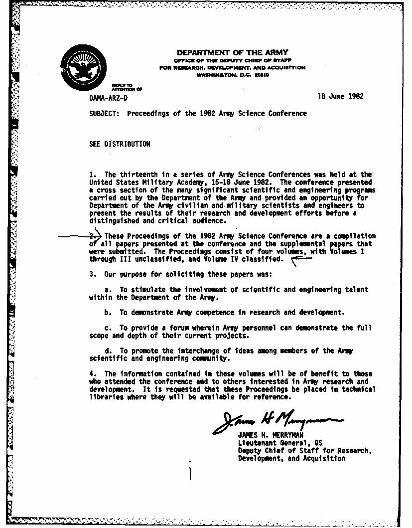
DAMA-ARZ-D 18 June 1982
SUBJECT: Proceedings of the 1982 Army Science Conference
SEE DISTRIBUTION
1. The thirteenth in a series of Armr Science Conferences was held at theUnited States Military Acade#y, 15-18 June 1982. The conference presenteda cross section of the many significant scientific and engineering programscarried out by the Department of the ArmW and provided an opportunity forDepartment of the Army civilian and military scientists and engineers topresent the results of their research and development efforts before adistinguished and critical audience.
---- a These Proceedings of the 1982 Arw Science Conference are a compilationokll papers presented at the conference and the suppl emental papers thatwere submitted. The Proceedings consist of four volumes, with Volumes Ithrough III unclassified, and Volume IV classified.
*5* 3. Our purpose for soliciting these papers was:a. To stimulate the involvement of scientific and engineering talent
within the Department of the Arm.
b. To demonstrate Army competence in research and development.
c. To provide a forum wherein Army personnel can demonstrate the fullscope and depth of their current projects.
d. To promote the interchange of ideas among members of the Armyscientific and engineering comunity.
4. The information contained in these volumes will be of benefit to those|,11 who attended the conference and to others interested in Army research and
development. It is requested that these Proceedings be placed in technicallibraries where they will be available for reference.
H. MERRYMANLieutenant General, GSDeputy Chief of Staff for Research,
* Development, and Acquisition
*1
DISTRIBUTION:Office, Under Secretary of Defense for Rsch & Engineering, Wash, DC 20310HQDA, ODCSRDA, ATTN: DAMA-ARZ-A, Washington, DC 20310HQDA, ODCSRDA, ATTN: DAMA-ARZ-D, Washington, DC 20310HQDA, Deputy Chief of Staff for Logistics, Washington, DC 20310HQOA, Deputy Chief of Staff for Operations, Washington, DC 20310HQDA, Deputy Chief of Staff for Personnel, Washington, DC 20310HQDA, Asst Chief of Staff for Automation and Cow unication, Wash, DC 20310HQDA, Assistant Chief of Staff for Intelligence, Washington, DC 20310HQDA, Office of the Chief of Public Affairs, Washington, DC 20310Office of the Surgeon General, ATTN: DASG-RDZ, Washington, DC 20310Office, Chief of Engineers, ATTN: DAEN-RDZ-A, Washington, DC 20314Office, Chief of Engineers, ATTN: DAEN-RDZ-B, Washington, DC 20314Office, Chief of Engineers, ATTN: DAEN-RDM, Washington, DC 20314COMMANDERS/DIRECTORSUS ArW Ballistic Missile Defense Systems Comand, Huntsville, AL 35807US Arqi Computer Systems Comand, Ft. Belvoir, VA 22060US Aroq Concepts Analysis Agency, Bethesda, MDUS Arm. Operational Test and Evaluation Agency, Falls Church, VA 22041fUS Are' Nat Dev & Readiness Cod, ATTN: DRCDRA-ST, Alexandria, VA 22333US Ary Nat Dev & Readiness Cod, ATTN: DRCLD, Alexandria, VA 22333US Army Armment RID Cmd, Dover, NJ 07801Ballistic Research Lab, Aberdeen Proving Ground, ") 21005Chemical Systems Lab, Aberdeen Proving Ground, M'D 21010Large Caliber Weapons Systems Lab, Dover, W) 07801Fire Control & Sall Caliber Weapons Systems Lab, Dover, NJ 07801US ArW Aviation RID Cmd, St. Louis, NO 63166USARTL, mes Research Center, boffett Field, CA 94035USARTL, Aeromchanics Lab, Noffett Field, CA 94035USARTL, Applied Technology Lab, Ft. Eustis, VA 23604USARTL, Propulsion Lab, Cleveland, OH 44135USARTL, Structures Lab, Hampton, VA 22665US ArW Avionics RID Activity, Ft. Nomuth, NJ 07r-US Armv Aviation Engineering Flight Activity, Edwaw,- - CA 93523
US Army Comnunications & Electronics Cud, Ft. Norutt, '703Center for Communications System, Ft. Nonmouth, NJ 0,iUV3Center for Tactical Couter Systems, Ft. Nomouth, NJ 07703Center for Systems Engineering & Integration, Ft. Nomouth, NJ 07703US ArvW Electronics RID Comand, Adelphi, ND 20783A tospheric Sciences Lab, White Sands Missile Range, 1N 88002Combat Surveillance & Target Acquisition Lab, Ft. Ntouth, NJ 07703Electronics Technology & Devices Lab, Ft. Nonmouth, NJ 07703Electronics Warfare Lab, Ft. Nameath, NJ 07703Ofc of Missile Electronic Warfare, White Sands Missile Range, M 88002Harry Diamd Laboratories, Adelphi, NO 20783Night Vision & Electro-Optics Lab, Ft. Belvoir, VA 22060Signals Warfare Lab, Vint Hill Farms Station, VA 22186US ArV Missile Comand, Redstone Arsenal, AL 35896-S ArW Missile Lab, Redstone Arsenal, AL 35898US Arm Nobility Equipment RD Command, Ft. Belvoir, VA 22060
2
~7;
US Army Natick Laboratories, Natick, MA 01760US Army Tank-Automotive Command, Warren, MI 48090Tank-Automotive Systems Lab, Warren, MI 48090Tank-Automotive Concepts Lab, Warren, MI 48090
US Army Test & Evaluation Command, Aberdeen Proving Ground, MD 21005US Army Aberdeen Proving Ground, Aberdeen Proving Gnd, MD 21005US Army Dugway Proving Ground, Dugway, UT 84022US Army Electronic Proving Ground, Ft. Huachuca, AZ 85613US ArmW Tropic Test Center, APO Miami 34004US Army White Sands Missile Range, White Sands Missile Range, M 88002US Army Yuma Proving Ground, Yuma, AZ 85364
US Army Research Office, Research Triangle Park, NC 27709US Army Materials & Mechanics Research Center, Watertown, MA 02172US Army Human Engineering Lab, Aberdeen Proving Ground, MD 21005US Army Mat Systems Analysis Activity, Aberdeen Proving Ground, MD 21005US Army Foreign Science A Tech Center, Charlottesville, VA 22901US Army Research, Development & Standardization Group (Europe)
4-. US Army Satellite Communications Agency, ATTN: DRCPM-SC-11, FortMornmouth, NJ 07703
US Army Training & Doctrine Cmd, ATTN: ATCD, Ft. Monroe, VA 23651US Army Health Services Command, Ft. Sam Houston, TX 78234Institute of Surgical Research, Ft. Sam Houston, TX 78234
US Army Medical R&D Command, Fort Detrick, Frederick, MD 21701Aeromedical Research Lab, Ft. Rucker, AL 36362Institute of Dental Research, WRAMC, Washington, DC 20012Letterman Army Inst of Research, Presidio of San Francisco, CA 94129Medical Bioengineering R&D Lab, Frederick, NO 21701Medical Rsch Inst of Chemical Defense, Aberdeen Proving Gnd, ND 21010Medical Rsch Inst of Environmental Medicine, Natick, MA 01760Medical Rsch Inst of Infectious Diseases, Frederick, NO 21701Walter Reed Army Inst of Research, Washington, DC 20012Walter Reed Army Medical Center, Washington, DC
Armed Forces Radiobiology Rsch Inst, Bethesda, MD 20814US Army Cold Regions Rsch & Eng Lab, Hanover, NHUS Army Construction Eng Rsch Lab, Champaign, ILUS Army Engineer Topographic Labs, Ft. Belvoir, VA 22060US Army Engineer Waterways Experiment Station, Vicksburg, MS 39180US Army Rsch Inst for the Behavioral & Social Sciences, Alex, VA 22333AR! Field Unit, Ft. Benjamin Harrison, IN 46216AR! Field Unit, Ft. Sill, OK 73603AR! Field Unit, Presidio of Monterey, CA 93940
COMMANDANTS:Acada of Health Sciences, ATTN: HSHA-CDM Ft. Sam Houston, TX 78234US Army Air Defense School, ATTN: ATSA-CDN-A, Ft. Bliss, TX 79916
. US Army Armor Center, ATTN: ATZK-CD-SD, Ft. Knox, KY 40121US Army Chemical School, ATTN: ATZN-CM-CS, Ft. McClellan, AL 36205US Army Engineer School, ATTN: ATZA-CD, Ft. Belvoir, VA 22060US ArW Field Artillery School, Ft. Sill, OK 73503US Army Infantry School, Ft. Benning, GA 31905US Army Intelligence Center and School, Ft. Huachuca, AZ 85613
3
, ' -1t! -k =;/' %~~~~~~~~.. .......%;- ,,.........•. ,- . .. .. . .. " -. . . . ........ ,
US Army Logistics Center, Ft. Lee, VA 23801US ArW Ordnance Center and School, Aberdeen Proving Gnd, MD 21005US AroW Signal Center, Ft. Gordon, GA 30905US ArW Transportation School, ATTN: ATSP-CD-CS, Ft. Eustis, VA 23604SUPERINTENDENT:US ArW Military Acadeqy, ATTN: Technical Library, West Point, NY 10996
COPIES FURNISHED:Defense Advanced Research Projects Agency, Arlington, VA 22209Defense Technical Information Center, Alexandria, VA 22209The Arqy Library, ATTN: ANRAL, Washington, DCChief, US Arwy Field Office, HQ AFSC/SDOA, Andrews AFB, MD 20331Cdr, HQ Fort Huachuca, ATTN: Tech Reference Div, Ft. Huachuca, AZ 85613Cdr, 1st COSCOM, HHC/SOTI, Ft. Bragg, NC 28303Naval Air Systems Command (Code 310-A), Washington, DC 20361Naval Research Library (Code 2627) Washington, DC 20361Office of Naval Research (Code 102, Arlington, VA 22217HQ US Marine Corps (Code RD-1), Washington, DC 20380Air Force Systems Command, Andrews AFS, Washington, DC 20331Lawrence Livermore Lab, Univ of California, Livermore, CA 94550Los Alamos Scientific Lab, Los'Alamos, N4 87544Southwest Research Institute, San Antonio, TX 78228United Nations Library, New York, NY 10017
4

PROCEEDINGS
OF THE
1982 ARMY SCIENCE CONFERENCE
UNITED STATES MILITARY ACADEMY
WEST POINT, NEW YORK
15-18 JUNE 1982
VOLUME I
Principal Authors A through G
DTIC TABunannounoedjustfloario
Distribution/ *odo
AailabilitV Codes0'Avail and/or NgCI
Dist. Special
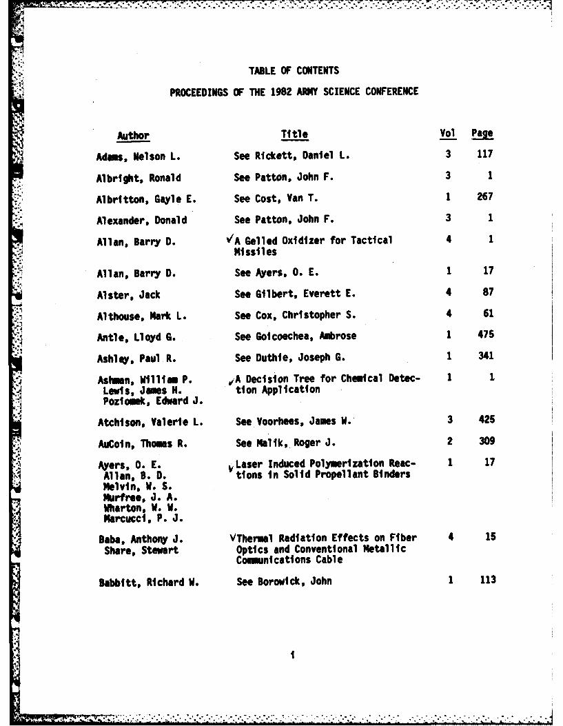
TABLE OF CONTENTS
PROCEEDINGS OF THE 1982 ARMY SCIENCE CONFERENCE
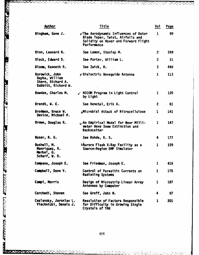
Author Title Vol Page
Adams, Nelson L. See Rickett, Daniel L. 3 117
Albright, Ronald See Patton, John F. 3 1
Albritton, Gayle E. See Cost, Van T. 1 267
Alexander, Donald See Patton, John F. 3 1
Allan, Barry D. VA Gelled Oxidizer for Tactical 4 1Missiles
Allan, Barry D. See Ayers, 0. E. 1 17
Alster, Jack See Gilbert, Everett E. 4 87
Althouse, Mark L. See Cox, Christopher S. 4 61
Antle, Lloyd G. See Goicoechea, Ambrose 1 475
Ashley, Paul R. See Duthie, Joseph G. 1 341
Ashman, W111am P. ,A Decision Tree for Chemical Detec- 1 1Lewis, James H. tion ApplicationPoziomek, Edward J.
Atchison, Valerie L. See Voorhees, James W. 3 425
AuCoin, Thomas R. See Malik, Roger J. 2 309
Ayers, 0. E. Laser Induced Polymerization Reac- 1 17Allan, B. D. tions in Solid Propellant BindersMelvin, N. S.Nurfree, J. A.Wharton, W. W.Marcucci, P. J.
Baba, Anthony J. VThermal Radiation Effects on Fiber 4 isShare, Stewart Optics and Conventional Metallic
Comunications Cable
Babbitt, Richard W. See Borowick, John 1 113
II
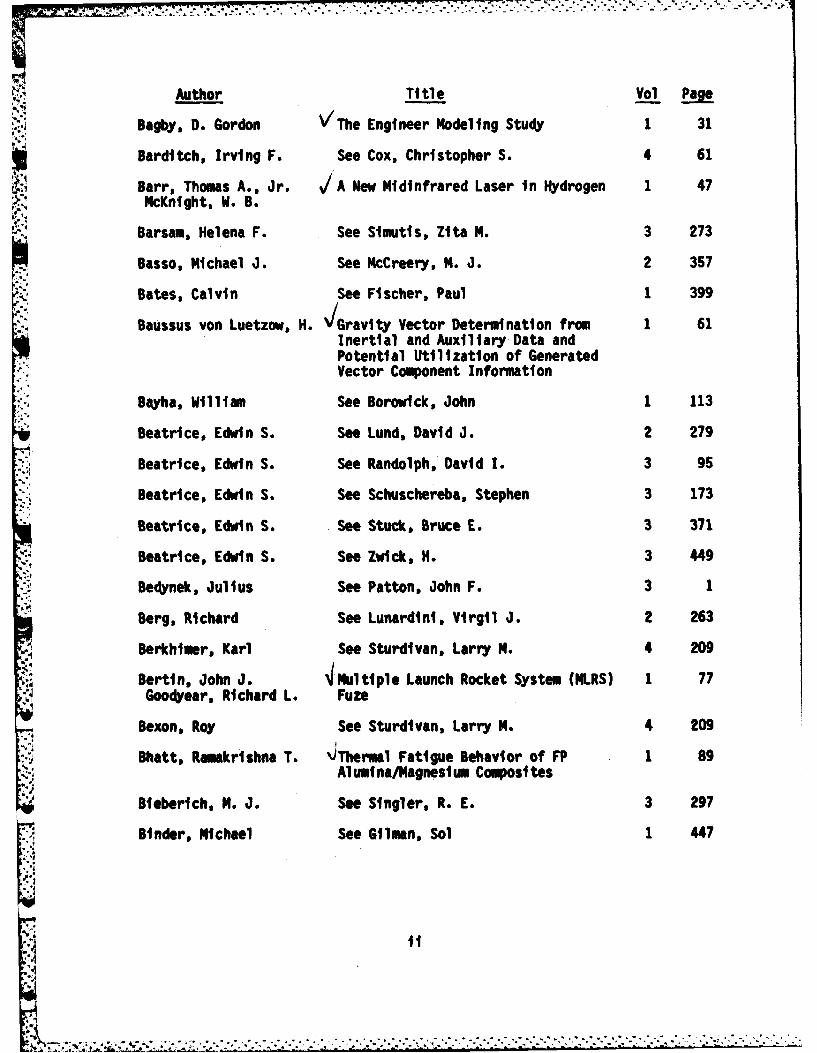
Author Title Vol PageBagby, D. Gordon VThe Engineer Modeling Study 1 31
Barditch, Irving F. See Cox, Christopher S. 4 61
Barr, Thomas A., Jr. A New Midinfrared Laser in Hydrogen 1 47McKnight, W. B.Barsam, Helena F. See Simutis, Zita M. 3 273
Basso, Michael J. See McCreery, M. J. 2 357
Bates, Calvin See Fischer, Paul 1 399
Baussus von Luetzow, H. "Gravity Vector Determination from 1 61Inertial and Auxiliary Data andPotential Utilization of GeneratedVector Component Information
Bayha, Willim See Borowick, John 1 113
Beatrice, Edwin S. See Lund, David J. 2 279
Beatrice, Edwin S. See Randolph, David 1. 3 95
Beatrice, Edwin S. See Schuschereba, Stephen 3 173
Beatrice, Edwin S. See Stuck, Bruce E. 3 371
Beatrice, Edwin S. See Zwick, H. 3 449
Bedynek, Julius See Patton, John F. 3 1
Berg, Ri chard See Lunardi ni, Virgil J. 2 263
Berkhimer, Karl See Sturdivan, Larry M. 4 209
Bertin, John J. VMultiple Launch Rocket System (MLRS) 1 77Goodyear, Richard L. Fuze
Bexon, Roy See Sturdivan, Larry M. 4 209
Bhatt, Ramkrishna T. 'Thermal Fatigue Behavior of FP 1 89Alumina/Magnesium Composites
Bieberich, M. J. See Singler, R. E. 3 297
Binder, Michael See Gilman, Sol 1 447
, .1
Author Title Vol Page
Bingham, Gene J. vThe Aerodynamic Influences of Rotor 1 99Blade Taper, Twist, Airfoils andSolidity on Hover and Forward FlightPerformance
Bnn, Leonard N. See Lemon, Stanley N. 2 249
Black, Edward D. See Porter, William L. 3 31
Bloom, Kenneth R. See Zwick, H. 3 449
Borowick, John VDielectric Waveguide Antenna 1 113Bayha, WilliamStern, Richard A.Babbitt, Richard W.
Bowden, Charles M. y* MICOM Program in Light Control 1 125by Light
Brandt, W. E. See Henchal, Erik A. 2 61
Brodman, Bruce W. fp)icrobial Attack of Nitrocellulose 1 141Devine, Michael P.
Brown, Douglas R. vAn Empirical Model for Near Milli- 1 147meter Wave Snow Extinction andBackscatter
Buser, R. G. See Rohde, R. S. 4 177
Bushell, M. I4 urora Flash X-Ray Facility as a 1 159Nanriquez, R. Source-Region EMP SimulatorMerkel, G.Scharf, W. D.
Cempana, Joseph E. See Friedman, Joseph E. 1 415
Campbell, Donn V. Control of Parasitic Currents on 1 175Radiating Systems
Campi, Morris Design of Microstrip Linear Array 1 187Antennas by Computer
Carchedi, Steven See Groff, John N. 4 97
Caslavsky, Jaro.lav L. Resolution of Factors Responsible 1 201Viechnicki, Dennis J. for Difficulty in Growing Single
Crystals of YAG
ttt
................................
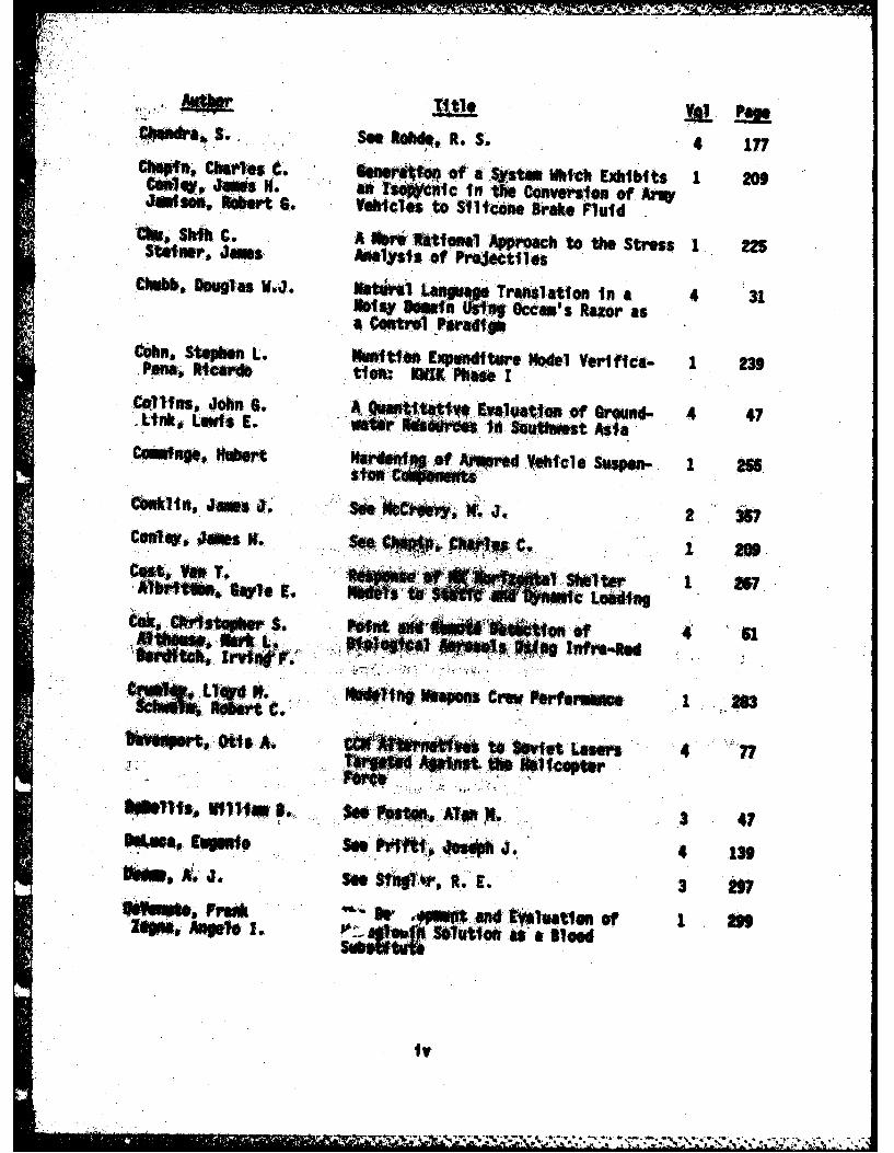
U ~ Titi I*! PaL* ChefrawSo See bR~. s. 4 27
C.eiCe~s. qrte~o a ~tmWhich Exhibits 1I 0Celq J~sK.atIscnc in aversion of Arqy20JONEson, Robert G. Vehicles9 to Silicone Brake Fluid
C na Shik toC A Oar* tttiayal Approach to the Stress 1 22Steinr, Jams Analysis of PrejectilesChabb, Douglas W. tthn La"pg Translation in a 4 31
Uily hiunUis ccas's Razor asa Contro Pradigm
COhn, Stephen L. Xmition Eeontitur e Mdel Verlifca. 1I 3Penw, Ricardo tion: 11(1 Phase 23CqOiws, John s. Aqu ttiqt~utiu fGon- 4 4.ivft, Lewis I. Ee ta.t intV Salti AsO' IaU.4
Cen*ge "Wbert Hedf f $vn4Vehicle Suspen., 1 2$.Sto" Cbakhls, Jass J.a tctel . 2 35
Celq Jas K.See 1 *0Cost, Va T.
MSf'lwwtg Cre, wefors. 1 -283
uft"PtvOttsAAiewt tho SoietcLaers7
Sfhs~VihaB. Se etpA1hs$. 3 47pan,# Soenw~t-o- 4 139
km. 3.See SfR~r t E.. 3 29
11e11s,0 Frp" I.I 4 ttinew ltonO
Its.
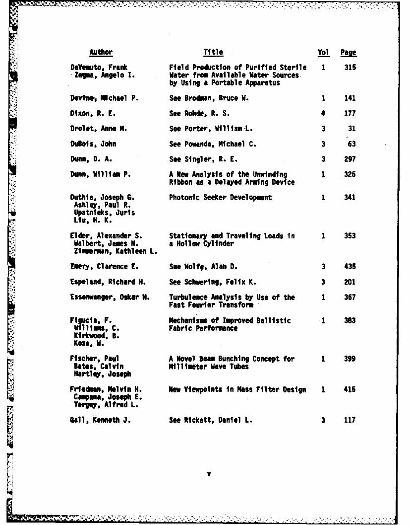
AuhrTitle Vol Pag
DeVenuto, Frank Field Production of Purified Sterile 1 315Zegna,, Angelo 1. Water from Available Water Sources.
by Using a Portable Apparatus
Devtne, Uchasi P. See Brodman, Bruce W. 1 141
Dixon, R. E. See Rohde, R. S. 4 177
Drolet, Anne M. See Porter, William L. 3 31
Dulois, John See Powanda, Michael C. 3 63
Dunn, 0. A. See Singler, R. E. 3 297
Dunn, William P. A Now Analysis of the Unwinding 1 325Ribbon as a Delayed Arming Device
Duthie, Joseph G. Photonic Seeker Development 1 341Ashley, Paul R.Upatnieks, JurisLiu, H. K.
El der, Alexander S. Stationary and Travel ing Loads in 1 353Walbert, James N. a Hollow CylinderZimmerman, Kathleen L.
Emery, Clarence E. See Wol fe, Alan 0. 3 435
Espeland, Richard H. See Schvering, Felix K. 3 201
Essenwanger, Oskar N. Turbulence Analysis by Use of the 1 367Fast Fourier Transform
Figucia, F. Mechanisms-of Improved Ballistic .1 383illiamso C. Fabric PerformanceKirkwood, B.Kozo, W.
Fischer, Paul A Novel Beom Bunching Concept for 1 399Sates,, Calvin Millimeter Wave TubesHartley, Joseph
Friedman, Melvin H. New Viewpoints in Mass Filter Design 1 415Camana, Joseph E.Yergey, Alfred L.
Gall, Kenneth J. See Rickett, Daniel L. 3 117
V v
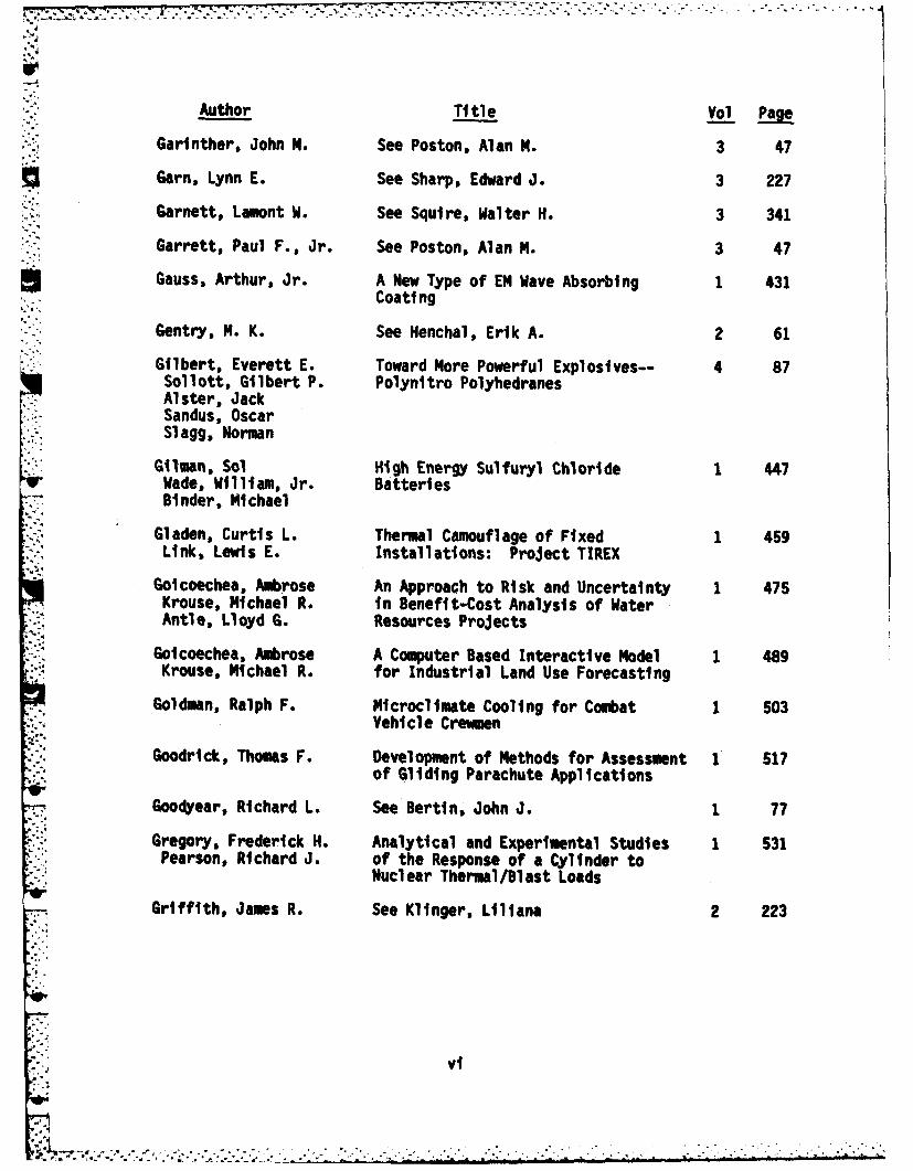
Author Title Vol ?
Garinther, John M. See Poston, Alan M. 3 47
Garn, Lynn E. See Sharp, Edward J. 3 227
Garnett, Lamont W. See Squire, Walter N. 3 341
Garrett, Paul F., Jr. See Poston, Alan M. 3 47
Gauss, Arthur, Jr. A New Type of EM Wave Absorbing 1 431Coating
Gentry, M. K. See Henchal, Erik A. 2 61
Gilbert, Everett E. Toward More Powerful Explosives-- 4 87Sollott, Gilbert P. Polynltro PolyhedranesAlster, JackSandus, OscarSlagg, Norman
Gilman, Sol High Energy Sulfuryl Chloride 1 447Wade, William, Jr. BatteriesBinder, Michael
Gladen, Curtis L. Thermal Camouflage of Fixed 1 459Link, Lewis E. Installations: Project TIREX
Golcoechea, Ambrose An Approach to Risk and Uncertainty 1 475Krouse, Michael R. in Benefit-Cost Analysis of WaterAntle, Lloyd G. Resources Projects
Goicoechea, Ambrose A Computer Based Interactive Model 1 489Krouse, Michael R. for Industrial Land Use Forecasting
Goldman, Ralph F. Microclimate Cooling for Combat 1 503,- Vehicle Crewmen
Goodrick, Thomas F. Development of Methods for Assessment 1 517
of Gliding Parachute Applications
Goodyear, Richard L. See Bertin, John J. 1 77
Gregory, Frederick H. Analytical and Experimental Studies 1 531Pearson, Richard J. of the Response of a Cylinder to
Nuclear Thermal/Blast Loads
Griffith, James R. See Klinger, Liliana 2 223
vi
Author Title ol !Me
Groff, John N. Armored Combat Vehicle Technology 4 97Mirabelle, Rosemary N. Using the HITPRO/DELACC Methodology
. Carchedi, Steven
. Groves, Michael G. See Twartz, John C. 3 411
Hagman, Joseph D. Maintaining Motor Skill Performance 2 1
Hardy, G. David, Jr. See Hiller, Jack H. 2 75
Harley, Samuel F. Data Compression for Transient 2 17- Measurements
Harris, Paul The Shock Front Rise Time in Water 2 33Presles, Henri-Noel
Hartley, Joseph See Fischer, Paul 1 399
Heavey, Karen R. See Nietubicz, Charles J. 2 425
Heberlein, David C. Detonation of Rapidly Dispersed 2 47Powders in Air
Heise, Carl J. See Mando, Michael A. 4 111
Henchal, Erik A. Rapid Identification of Dengue Virus 2 61McCown, J. N. Serotypes Using Monoclonal AntibodiesGentry, M. K. in an Indirect lImunofluorescenceBrandt, W. E. Test
Herren, Kenneth A. See Johnson, John L. 2 199
Hiller, Jack H. Design of a Small Unit Drill Training 2 75* Hardy, G. David System
Meliza, Larry L.
Hoidale, Glenn B. See Walters, Donald L. 4 239
Hollenbaugh, D. D. Quantification of Helicopter Vibra- 2 91tion Ride Quality Using AbsorbedPower Measurements
Howe, Philip M. A Theoretical Study of the Propaga- 2 109Kiwan, Abdul R. tfon of a Mass Detonation
Hsiesh, Jen-Shu See McCreery, M. J. 2 357
Hubbard, Roger W. Water as a Tactical Weapon: A 2 125Mager, Milton Doctrine for Preventing HeatKerstein, orris Casualties
vii
-- 7 . . . . -. ,* ***i' - . . . . . . . - - . - - -
Author Title Vol Page
Hutchings, Thomas D. Analysis of Small Caliber Manuever- 2 141able Projectile (SCMP) Concepts forHelicopter and Air DefenseApplications
Huxsoll, David L. See Twartz, John C. 3 411
Hynes, John N. Heuristic Information Processing as 2 157Jimarez, David S. Implemented in Target Motion Resolu-
tion Analysis of Radar Data
Hynes, Thomas V. Attenuation of High Intensity 2 171Reradiated Light by PhotochromicGlass
lafrate, Gerald J. Utilization of Quantum Distribution 2 177Functions for Ultra-Submicron DeviceTransport
Jamison, Keith A. See Thomson, George M. 3 385
Jamison, Robert G. See Chapin, Charles C. 1 209
Jenkins, Thomas See Lunardini, Virgil J. 2 263
Jenkinson, Howard A. CO2 Laser Waveguiding in GaAs MBE 2 189Zavada, John M. Layers
Jimarez, David S. See Iynes, John N. 2 157
Johnson, John L. Active Imaging of Range Targets at 2 199Herren, Kenneth A. 1.2 MillimetersMorgan, Robert L.Tanton, George A.
Johnson, Robert A. See Schwering, Felix K. 3 201
Kane, P. J. See Singler, R. E. 3 297
Kapsalis, John G. See Porter, William L. 3 31
Kerstein, Morris See Hubbard, Roger W. 2 125
Kirkwood, B. See Figucia, F. 1 383
Kittleson, John K. Holographic Interferometry Technique 2 209Yu, Yung H. for Rotary Wing Aerodynamics and Noise
%.
,........ .. .. . .. .. . .. .. . .. .. .
., - , .. . n * * . * -]1
Author Title Vol Page
Kiwan, Abdul R. See Howe, Philip M. 2 109
Klinger, Liliana Fluoropolymer Barriers to Stress 2 223Griffith, James R. Corrosion in Optical Fibers
Knudson, Gregory B. See Mikesell, Perry 2 385
Koulouris, T. N. See Singler, R. E. 3 297
Koza, W. See Figucia, F. 1 383
Kronenberg, Stanley Tactical Gamma and Fast Neutron 2 235Dosimetry with Leuko Dye OpticalWavegui des
Krouse, Michael R. See Goicoechea, Ambrose 1 475
Krouse, Michael R. See Goicoechea, Ambrose 1 489
Kunkel, Kenneth E. See Walters, Donald L. 4 239
LeDuc, James See Lemon, Stanley M. 2 249
* Lee, H. See Singler, R. E. 3 297
* Lemon, Stanley M. Isolation of Hepatitis A Virus from 2 249LeDuc, James the New World Owl Monkey: A NewBinn, Leonard N. Animal Model for Hepatitis A
Infections
Lewis, Danny H. See Setterstrom, Jean A. 3 215
Lewis, James H. See Ashman, William P. 1 1
Lieberman, Michael M. See Powanda, Michael C. 3 63
Link, Lewis E. See Collins, John G. 4 47
Link, Lewis E. See Gladen, Curtis L. 1 459
Liu, H. K. See Duthie, Joseph G. 1 341
Lunardini, Virgil J. The Mobility of Water in Frozen Soils 2 263Berg, RichardMcGaw, RichardJenkins, ThomasNakano, Yoshisuke01liphant, JosephO'Neill, KevnTice, Allan
ixi
",
- . " - - - -. -. ..... .. . . ..
Author Title Vol Page
Lund, David J. Bioeffects Data Concerning the Safe 2 279Beatrice, Edwin S. Use of GaAs Laser Training DevicesSchuschereba, Steven
Lund, David J. See Stuck, Bruce E. 3 371
Lund, David J. See Zwick, h. 3 449
Machuca, Raul Computer Detection of Low Contrast 2 293Targets
Mager, Milton See Hubbard, Roger W. 2 125
Malik, Roger J. The Planar Doped Barrier: A New 2 309AuCoin, Thomas R. Class of Electronic DevicesRoss, Rayumond L.Savage, Robert 0.
Mando, Michael A. Development of Armature Insulation 4 111Heise, Carl J. Technique for Compact, High Power
Al ternators
-- Manriquez, R. See Bushell, M. 1 159
Marchese, Vincent P. IR Algorithm Development for Fire 2 325
and Forget Projectiles
Marchionda, Kristine M. See Voorhees, James W. 3 425
Marcucci, P. J. See Ayers, 0. E. 1 17
Martel, C. James Development of a New Design Proced- 2 341ure for Overland Flow System
McCown, J. M. See Henchal, Erik A. 2 61
McCreery, M. J. Biologic Dosimetry for Nuclear 2 357Swenberg, Charles E. Environments by Electron ParamagneticBasso, Michael J. Resonance (EPR) MethodsConklin, James J.Hsieh, Jen-Shu
McDonough, John H. The Effects of Nerve Agents on 2 371Behavioral Performance and TheirModification with Antidotes andAntidote Combinations
McGaw, Richard See Lunardini, Virgil J. 2 263
X' 1q ,%,
f-- ! ... , .. ... . ... . .......... .... , : ... ,. i -.... , i -., ..
.. .. . .. ... , .. . . I I
Author Title Vol Page
McKnight, W. B. See Barr, Thomas A., Jr. 1 47
Meliza, Larry L. See Hiller, Jack H. 2 75
Melvin, W. S. See Ayers, 0. E. 1 17
Merkel, G. See Bushell, M. 1 159
Meyers, William E. See Setterstrom, Jean A. 3 215
Mikesell, Perry Plasmids of Legionella Species 2 385Knudson, Gregory B.
Miller, Miles C. Flight Instabilities of Spinning 2 393Projectiles Having Non-RigidPayloads
Mirabelle, Rosemary See Groff, John N. 4 97
Morgan, Robert L. See Johnson, John L. 2 199
Murfree, J. A. See Ayers, 0. E. 1 17
Murphy, Newel1 R. Armored Combat Vehicle Technology 2 409(ACVT) Program Mobility/AgilityFindings
Nakano, Yoshisuke See Lunardini, Virgil J. 2 263
Ni etubicz, Charles J. Computations of Projectile Magnus 2 425Sturek, Walter B. Effect at Transonic VelocitiesHeavey, Karen R.
Nolan, Raymond V. Explosives Detection Systems Employ- 2 441i ng Behaviorally Modified Rats asSensory Elements
Nomiyama, N. T. See Rohde, R. S. 4 177
Norton, M. C. See Rohde, R. S. 4 177
Obert, Launne P. See Ratches, James A. 4 163
O'Connell, Robert L. Soviet Land Arms Acquisition Model 4 125
O'Neill, Kevin See Lunardini, Virgil J. 2 263
Oliphant, Joseph See Lunardini, Virgil J. 2 263
xi
Author Ti tle Vol Page
Patton, John F. Aerobic Power and Coronary Risk 3 1Vogel, Jams A. Factors in 40 and Over AgedBedynek, Ju1 us Mil t -y PersonnelAlexander, DonaldAlbright, Ronald
Pearson, Richard J. See Gregory, Frederick H. 1 531
Pena, Ricardo See Cohn, Stephen L. 1 239
Phelps, Ruth H. Expert's Use of Information: 3 17Is It Biased?
Porter, William L. A Rationale for Evaluation and 3 31Kapsall s, John G. Selection of Antioxidants foretherby, Ann Marie Protection of Ration Items of
Drolet, Anne M. Different TypesBlack, Edward D.
Poston, Alan M. Human Engineering Laboratory Avia- 3 47Garrett, Paul F., Jr. tion Supply Class Ill/V MaterielDeBellis, William B. (HELAYS III/V) Field TestReed, Harry J.Garinther, John N.
Powanda, Michael C. Biochemical Indicators of Infection 3 63DuBois, John and Inflimtion in Burn InjuryVillarreal, YsidroLieberman, Michael M.Pruitt, Basil A., Jr.
Poziomek, Edward J. See Ashman, William P. 1 1
Presles, Henri-Noel See Harris, Paul 2 33
Prichard, Dorothy A. See Wolfe, Alan D. 3 435
Prifti, Joseph J. Development of Ballistic Spall- 4 139DeLuca, Eugenio Suppression Liner for M113 Armored
Personnel Carrier"4 Pruitt, Basil A., Jr. See Powanda, Michael C. 3 63
Ramsley, Alvin 0. Psychophysics of Modern Camouflage 3 79Yeomans, Walter G.
Randers-Pehrson, Glenn Nonaxisyimetric Anti-Armor Warheads 4 153
xii
..................................
Author Title Vol Page
Randolph, David I. Laser Flash Effects: A Non-Visual 3 95Sciweisser, Elmer T. Phenomenon?Beatrice, Edwin S.Randolph, Thomas C. See Rickett, Daniel L. 3 117
Ratches, James A. FLIR/I4 Radar vs FUR Alone 4 163
Obert, Luanne P.
Reed, Harry J. See Poston, Alan N. 3 47
Reed, Lockwood W. Voice Interactive Systems Technology 3 107Avionics (VISTA) Program
Rickett, Daniel L. Differentiation of Peripheral and 3 117I-Adams, Nelson L. Central Actions of Soman-ProducedGall, Kenneth J. Respiratory ArrestRandolph, Thomas C.Rybczynski, Siegfried
Rohani, Behzad Probabilistic Solution for One- 3 131Dimensional Plane Wave Propagationin Homogeneous Billnear Hysteretic
Rohde, R. S. Laser Technology for Identification 4 177Buser, R. G. on the Nodern BattlefieldNorton, N. C.Dixon, R. E.
"J Nomiyame, N. T.Chandra, S.
Rokkos, Nikolaus See Schwtulmg, Feix K. 3 201
Ross, Raymond L. See Malik, Roger J. 2 309
Roth, John A. Measured Effects of Tactical Smoke 3 147and Dust on Performance of a HighResolution Infrared Imaging System
Rybczynski, Siegfried See Rickett, Daniel L. 3 117
Salomon, Mark Properties of SOC12 Electrolyte 3 163Solutions
Sandus, Oscar See Gilbert, Everett E. 4 87
Saunders, J. Peter See Tartzi, John C. 3 411
xiii
. .- , ". . .- ... -. - . . .*-. . . . -. - . . .. .. . ... . . . . . .
Author Title Vol Pg
Savage, Robert 0. See Malik, Roger 3. 2 309
Scharf, W. 0. See Bushell, N. 1 159
Schmeisser, Elmar T. See Randolph, David 1. 3 95
Schiaschereba, Stephen Autoradiography of Primate Retina 3 173Beatrice,, Edwin S. After Q-Svitched Ruby Laser
Radiation
Schuschereba, Stephen See Lund, David J.* 2 279
Schwalm, Robert C. See Crumay, Lloyd N. 1 283Schwartz, Paul N. Methods for Evaluating Gun-Pointing 3 189
Angle Errors and Miss DistanceParameters for an Air Defense GunSystem
Schwering, Felix K. Effects of Vegetation and Battlefield 3 201Johnson, Robert A. Obscurants on Point-to-Point Trans-Rokkosq Nikolaus mission in the Lower Millimeter WaveWhibon, Gerald M. Region (30-60 ONO)Violette, Edhond 3.Espeland, Richard H.
Selvaraju, 6. See Twartz, John C. 3 411
Setterstrom, Jean A. Controlled Release of Antibiotics 3 215Tice, Thomas R. from Biodegradable Microcapsules
-Lewi s, Danny H. for Wound Infection ControlMeyers, William E.
Share, Stewart See Saba, Anthony 3. 4 1s
Sharp, Edward J. Electrical Properties of Heated 3 227Barn, Lynn E. Dielectrics
Sheldon, William 3. The Development and Production 4 193of the Tungsten Alloy N74 Grenade
Shiral Akira See Tvartz, John C. 3 411
Shuely, Wendel 3. A New Interactive,, Computer-Controlled 3 243Method for Investigating ThermalReactions for the 'Thermodetoxifica-tion' and Resource Recovery of SurplusChemicals
xlv
'-7
4
Author Ti tle Vol Pa
*1 Silverstein, Joseph D. Hear Millimeter Wave Radiation 3 259from a Gyromonotron
Siumtis, Zita M. Terrain Visualization by Soldiers 3 273Barsm, Helena F.
Sindoni, Orazio I. Calculation on Optical Effect of 3 283Matter from First Principles UsingGroup Theoretical Techniques
Singler, R. E. Synthesis and Evaluation of 3 297Koulouris, T. N. Phosphazene Fire Resistant FluidsDeome, A. J.Lee, H.Dunn, D. A.Kane, P. J.Bieberich, M. J.
Slagg, Norman See Gilbert, Everett E. 4 87
Smith, Alvin A Method of Polymer Design and 3 309Synthesis for Selective InfraredEnergy Absorption
Sollott, Gilbert P. See Gilbert, Everett E. 4 87
Spellicy, Robert L. See Watkins, Wendell R. 4 249
Spoonamore, Janet H. CAEADS--Computer Aided Engineering 3 325and Architectural Design System
Squire, Walter H. Visco-Elastic Behavior of Incendiary 3 341Garnett, Lamont W. Compositions Under Ballistic Loading
Steiner, James See Chu, Shih C. 1 225
Sterling, Bruce S. The Relationship Between Company 3 357Leadership Climate and ObjectiveMeasures of Personnel Readiness
Stern, Richard A. See Borowick, John 1 113
Stuck, Bruce E. Ocular Flash Effects of Relatively 3 371Lund, David J. "Eye Safe" LasersBeatrice, Edwin S.
Sturdivan, Larry M. General Bullet Incapacitation and 4 209Bexon, Roy Design ModelBerkhimer, Karl
xv
'-. iAuthor Title Vol Page4 -
4.. Sturek, Walter B. See Nietublcz, Charles J. 2 425
Swenberg, Charles E. See McCreery, M. J. 2 357
Tanton, George A. See Johnson, John L. 2 199
Thomon, George . In-Bore Propellant Media Density 3 385Jamison, Keith A. Measurements by Characteristic
X-Ray Radiography
Throop, Joseph F. A Fracture and Ballistic Penetration 3 397
Resistant Laminate
Tice, Allan See Lunardini, Virgil J. 2 263
Tice, Thomas R. See Setterstrom, Jean A. 3 215
Turetsky, Abraham L. Advances In Multispectral Screening 4 225
Twartz, John C. Doxycycline Prophylaxis of Scrub 3 411Shirai, Akira TyphusSelvaraJu, G.Saunders, J. PeterHuxsoll, David L.Groves, Michael G.
Upatnieks, Juris See Duthie, Joseph 6. 1 341
Verdier, Jeff S. See Wolfe, Alan D. 3 435
Viechnicki, Dennis J. See Caslavsky, Jaroslav L. 1 201
Villarreal, Ysidro See Powanda, Michael C. 3 63
Violette, Edmond J. See Schwering, Felix K. 3 201
Vogel, James A. See Patton, John F. 3 1
Voorhees, James W. Speech Comand Auditory Display 3 425Marchionda, Kristine System (SCADS)Atchison, Valerie L.
Wade, William L., Jr. See Gilmmn, Sol 1 447
Walbert, James N. See Elder, Alexander S. 1 353
Walters, Donald L. Optical Turbulence within the 4 239Kunkel, Kenneth E. Convective Boundary LayerNoidale, Glenn B.
xvi
..
Author Ti tle Vol !!eWatkins, Wendell R. Simulated Plume Radiative Transfer 4 249White, Kenneth 0. MeasurementsSpellicy, Robert L.
Wetherby, Anne Marie See Porter, William L. 3 31Wharton, W. W. See Ayers, 0. E. 1 17
White, Kenneth 0. See Watkins, Wendell R. 4 249
Whitman, Gerald M. See Schwering, Felix K. 3 201
Williams, C. See Figucia, F. 1 383
Wolfe, Alan D. Studies on Butyrylcholinesterase 3 435Emery, Clarence E. InhibitorsVerdier, Jeff S.Prichard, Dorothy A.
Yeomans, Walter G. See Ramsley, Alvin 0. 3 79Yergey, Alfred L. See Friedman, Melvin H. 1 415
Yu, Yung H. See Kittleson, John K. 2 209
Zavada, John M. See Jenkinson, Howard A. 2 189
Zegna, Angelo I. See DeVenuto, Frank 1 299Zegna, Angelo I. See DeVenuto, Frank 1 315
ZtNerman, Kathleen L. See Elder, Alexander S. 1 353Zwick, H. Laser Ocular Flash Effects 3 449Bloom, Kenneth R.Lund, David J.Beatrice, Edwin S.
xvii-a . . . . . . . . . . .
*ASHMAN, LEWIS, 4 POZIOMEK
A DECISION TREE FOR CHEMICAL DETECTION APPLICATION (U)
*WILLIAM P. ASHMAN, Mr.
JAMES H. LEWIS, Mr.EDWARD J. POZIONEK, PhD.
CHEMICAL SYSTEMS LABORATORY, USAARRADCOMABERDEEN PROVING GROUND, MD 21010
I. Introduction
In chemical detection research, there is considerable interest in find-ing reactions and reagents that will be active in solid state in detectingchemical agents and agent simulants at low concentrations. The applicationof the reagents and their interactions would be for use in detection devicessuch as detector tubes, personnel dosimeters, or solid state coatings forvarious types of microsensor devices such as piezoelastic crystals.
In this research, a major problem is the development of a reagent andits interaction that is specific for a chemical agent or simulant withoutinterference from other chemicals in the environment. In solid state de-tection research, there has been no base of information from which to drawin designing coatings that will be specific for particular chemicals. Thisis true generally irrespective of the nature of the chemical to be detected.Although much may be known about the chemistry of a particular molecule insolution, this same knowledge cannot be transferred routinely in predictingsolid state reactions.
In finding new solid state reagents and interactions, the classicalprocedure is to screen randomly many compounds until the desired detectionis obtained. Not only is this screening expensive; but in most cases, itis unsuccessful. Also, using this mass screen procedure, once a suitableagent/detector reagent interaction is developed, there is no way of pre-dicting what interferences there will be without undertaking another major
'A screening process.
This paper describes research in the des4.gn of indandione derivativesthat can be used as detector reagents and as coatings for solid-state detec-tion purposes. A chemometrics analysis (statistical, discriminant) wasSperformed of the results obtained with one of the reagents, 2-diphenylacetyl.1,3-indandione-1 (P-dinethylaminobenzaldazine). Chemical structural and
"!1
. . . . .gr ,.--.J-- --..-- . r- " --- " --- " * . ' " ' " " "-
*ASHIA, LEWIS & POZIOMEK
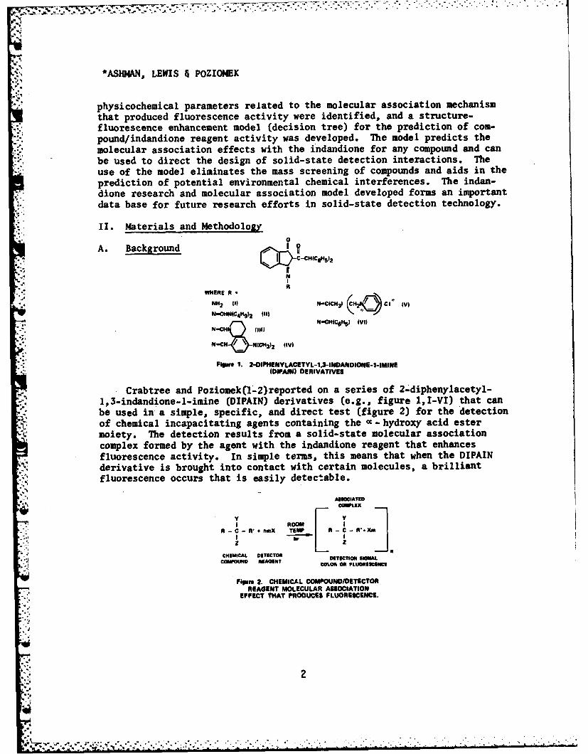
physicochemical parameters related to the molecular association mechanismthat produced fluorescence activity were identified, and a structure-fluorescence enhancement model (decision tree) for the prediction of con-pound/indandione reagent activity was developed. The model predicts themolecular association effects with the indandione for any compound and canbe used to direct the design of solid-state detection interactions. Theuse of the model eliminates the mass screening of compounds and aids in theprediction of potential environmental chemical interferences. The indan-
.1 dione research and molecular association model developed forms an importantdata base for future research efforts in solid-state detection technology.
II. Materials and Methodology
A. Background I _ V
RWHERE R -
NH 2 I" N-C(CH 3) (CI (V"" 4"912 till ,
-- ," / %N-<:HICgig ) (VI)
.'.N-CH!&I ( IV'
Figue 1. 2-DIPHENYLACETYL-1.3-INDANDIONE-1-IMINE(DIPAIN) DERIVATIVES
Crabtree and Poziomek(1-2)reported on a series of 2-diphenylacetyl-1,3-indandione-l-imine (DIPAIN) derivatives (e.g., figure 1,I-VI) that canbe used in a simple, specific, and direct test (figure 2) for the detectionof chemical incapacitating agents containing the ac- hydroxy acid estermoiety. The detection results from a solid-state molecular associationcomplex formed by the agent with the indandione reagent that enhancesfluorescence activity. In simple terms, this means that when the DIPAINderivative is brought into contact with certain molecules, a brilliant
, S.fluorescence occurs that is easily detectable.
* ASSOCIATED
ROOM IIII-C - A,+ MX TEMP R -C - W.XmI
CHEMICAL DETECTOR DETECTION UWEA.COIPOUINO REAGENT oT. OR SIGNL
Figure 2. CHEMICAL COMPOUND/DETECTORREAGENT MOLECULAR ASSOCIATION
EFFECT THAT PRODUCES FLUORESCENCE.
. .
A . . . . .-,. . . . .. . . . . . . .-• . . . - ° • . :, - . . . . . . .

*ASHMAN. LEWIS 5 POZIO14EK
Screening studies for compound detection with 6 of the DIPAIN reagentsindicated that each reagent has a distinctive fluorescence activity pro-file. For the compounds tested, a reagent may give a sensitive fluores-cence (a strong enhancement) with some but only a moderate to no responsewith others (figure 3).
FLUORESCENCE INTENSITYa
CMPDCOMPOUND ALONE I II III IV V VI
INSECTICIDESDOT NEG M S MS S NEG MCHLORDANE M Mb M MS S
c Wd M
HEPTACHLOR M W M M SC W MTOXAPHENE M W M M Sb W M
RODENTICIDEWARFARIN W M Sb M MSc Mb M
HERBICIDEPHENOXYACETIC ACID M NEG MS Sb WC MS M
MOBSERVED RELATIVE FLUORESCENCE: NEG. NO FLUORESCENCE; W.WEAK; M. MEDIUM; MS. MODERATELY STRONG; S. STRONG. OBSERVEDCOLOR IN AMBIENT LIGHT: b YELLOW: c ORANGE: d GREEN.
FIgure . COMPARISON OF FLUORESCENCE ENHANCEMENTEFFECTS OF DDT WITH DIPAIN DERIVATIVES.
The fluorescence enhancement detection method can be used on varioussurfaces; and the detection response varies with the reagent and surfaceused (figure 4).
FLUORESCENCE INTENSITY
SOLID SUPPORT I II III IV V VI
ALUMINA M M M S NEG SCELLULOSE S M W MS NEG MSGLASS FIBER M S MS S NEG MWHATMAN PAPER M M M S VW M
SILICA GEL W W - - -
OBSERVED RELATIVE FLUORESCENCE: NEG. NO FLUORE-SCENCE: VW. VERY WEAK; W. WEAK; M, MEDIUM; MS,MODERATELY STRONG; S, STRONG: -, NOT TESTED.
Figure 4. EFFECT OF SOLID SUPPORT ONFLUORESCENCE ENHANCEMENT WITH DDT.
For the purpose of extending the usefulness of the fluorescence en-hancement technique and to obtain data that might reveal more about themechanism of the molecular interaction responsible for the fluorescence,additional compound/indandione derivative interaction profiles of otherclasses of compounds (insecticides, rodenticides, amino acids, aliphatics,alcohols, nucleic acids, etc.) were determined. A comprehensive listingoF the reagents, test procedures, compound/detector reagent fluorescenceactivity profiles, methods of synthesis, and a chemometrics analysis todevelop compound/DIPAIN reagent structure fluorescence activity models havebeen reported.
I
*ASHMAN, LEWIS, & POZIOMEK
B. Materials and Detection Assay
The solid-solid molecular association fluorescence enhancement methodof detection (figure 2) is relatively simple and easy to use. It has anadvantage over other chemical detection methods in that it avoids chemicalreactions which usually require prolonged heating and/or concentrated acidor base to produce a detection signal. In this paper, DIPAIN IV, the p-dimethylaminobenzaldazine derivative, and its interactions are analyzed.
Approximately 750 compounds were tested with the DIPAIN IV reagent.The test procedure was as follows: liquid samples of the compounds to bedetected were spotted without dilution on Gelman ITLC glass fiber sheetsusing lIl disposable micropipettes. Solid samples were spotted as 10%solution (w/v) in tetrahydrofuran. Each sheet was lightly sprayed with theDIPAIN IV reagent solution (made up as a 0.1% (w/v)) solution in benzene(0.12g/l). After the solvent evaporated, the spots were scanned visuallyfor any change in color or fluorescence. A Chromato-Vue Cabinet with XX-1SC long wave (peak at 366nm) ultraviolet lamp (Ultraviolet Products, Inc.,San Gabriel, CA 91778)was used to check for fluorescence. A visual ob-servation was made, and the response was 'qualitativelyt categorized intoone of 8 groups (none; very weak; weak; weak medium; medium; medium strong;strong; absorbed). In the chemometrics analysis, the 8 groups were reduce;into 2 categories (unacceptable fluorescence; none, very weak, weak medium::medium, absorbed- and acceptable-fluorescence; medium strong, strong).
C. Chemometrics Analysis
A Chemometrics Sciences Section has been established at the ChemicalSystems Laboratory (CSL) to use the theoretical chemistry and computer-aided mathematical and statistical methods as a tool to aid the chemist inthe development of mechanistic models of compound activity. The followingsystematic approach was used:
(1) Identify by literature (3-6) and consultation with ex-perts the compound and reagent structural and/or physicochemical featuresthat theoretically relate to fluorescence and to the molecular associationeffects that may enhance or decrease fluorescence.
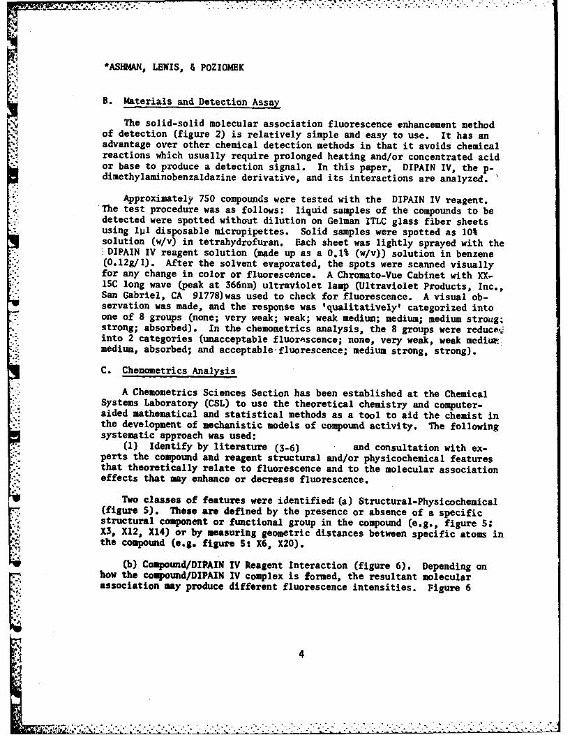
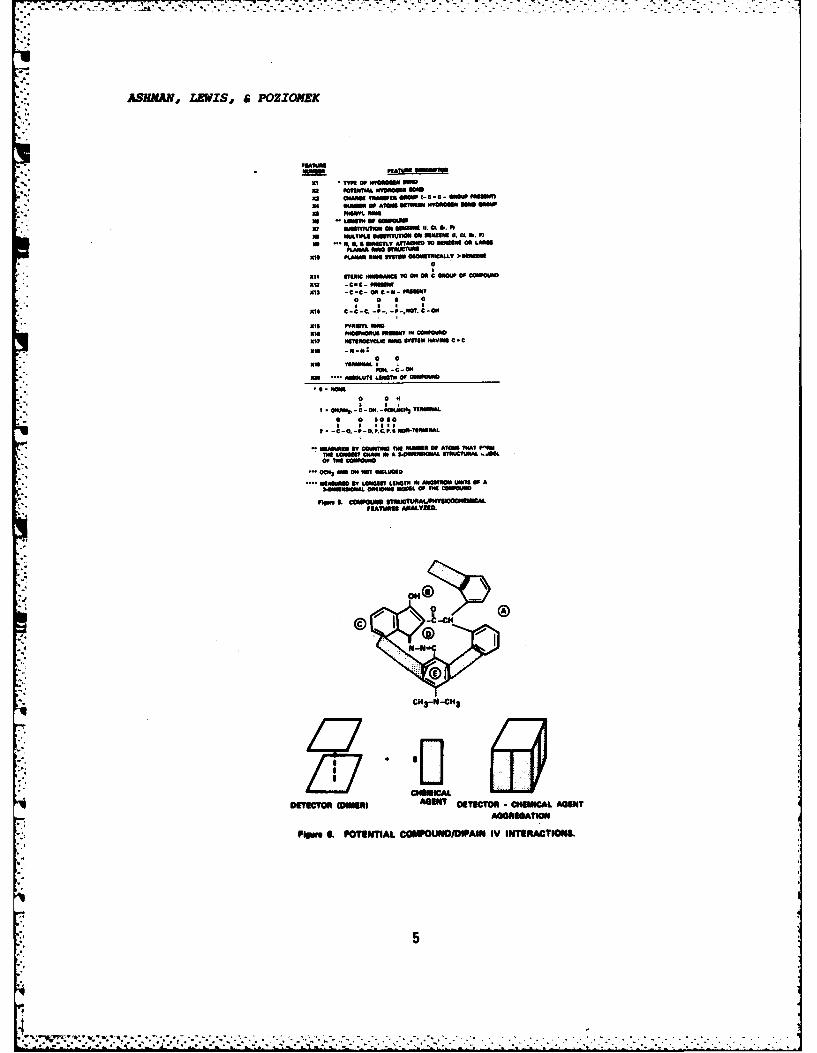
Two classes of features were identified: (a) Structural-Physicochemical(figure S). These are defined by the presence or absence of a specificstructural component or functional group in the compound (e.g., figure 5;X3, X12, X14) or by measuring geometric distances between specific atoms inthe compound (e.g. figure S: X6, X20).
(b) Compound/DIPAIN IV Reagent Interaction (figure 6). Depending onhow the compound/DIPAIN IV complex is formed, the resultant molecularassociation may produce different fluorescence intensities. Figure 6
4
ASBI4AN, LEVIS, 6 POZZONEC
3w ow*11 TKMwUa waw I- C -C - NOW panuX4 560 op~ ATUI OM UISCo~ 0 610" .11mg.
no LOAMIO OF I Is a..
5t WAIT" 0. S Ma Ill1.t CLAOI 6. F)lS 04"Tm SBUTT soswm .Ut6.F
al ftin *Me swams offamff""T > 461mM
III SISKI IKKSSIKCI To ON on C ~34 OF C
Mu -C*C- 'mowX13 -C-C- OR C-K- FKUES
O 0 0I I
RI1 C-C-C. -U- ,-K C-OK
XlI PYAOYI. RMK
:17 KITsKoevaCIC "asB $manl IAVUS C *C
0 0IlK 6t MN't
- 16150 0~
I . OkII~ - C - ON. -lSIMiI03 TIKKUDO.
a 0 10801. .C . P. COPCP. icoUK.TIKAt
MSD SV MWIKUM Il MlUMh OF ATOM MKAT UFKKTHE 1.016W 1115111 W A 3U61OKA1. SIKITIAL ..3KOf ISO COOSI
IM"St L*56 IN ANGP1 W~ OF AKIASIMO ST LLOmIt1111 KAIUO 611i
11pm 0.OMOUKO ST0UCTURALHIYSCCHIMFRATIJAIS ADEALMZD.
0 -M
c H -N 4H,
DESCIOR iua) AGENT DETECTOR HA- LAGN
Pipss SL POTENTIAL COMPOUNOIDIPAIN IV INTERACTIONS.
*ASIMAN, LEWIS POZIOMEK
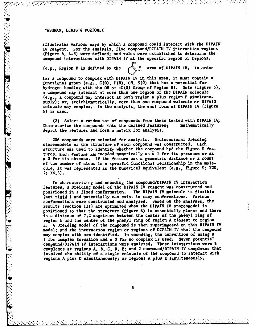
illustrates various ways by which a compound could interact with the DIPAINIV reagent. For the analysis, five compound/DIPAIN IV interaction regions(Figure 6, A-E) were defined; and rules were established to determine thecompound interactions with DIPAIN IV at the specific region or regions.
ON(e.g., Region B is defined by the 10 area of DIPAIN IV. In order
for a compound to complex with DIPAIN IV in this area, it must contain a
functional group (e.g., C(O), P(0), OH, S(O) that has a potential forhydrogen bonding with the OH or -C(O) Group of Region B). Note (figure 6),
a compound may interact at more than one region of the DIPAIN molecule(e.g., a compound may interact at both region A plus region E simultane-
ously); or, stoichiometrically, more than one compound molecule or DIPAINmolecule may complex. In the analysis, the enol form of DIPAIN IV (figure6) is used.
(2) Select a random set of compounds from those tested with DIPAIN IV,
Characterize the compounds into the defined features; mathematicallydepict the features and form a matrix for analysis.
206 compounds were selected for analysis. 3-dimensional Dreiding
stereomodels of the structure of each compound was constructed. Eachstructure was usei to identify whether the compound had the figure 5 fea-
tures. Each feature was encoded numerically as a 1 for its presence or asa 0 for its absence. If the feature was a geometric distance or a count
of the number of atoms in a specific functional relationship in the mole-cule, it was represented as the numerical equivalent (e.g., figure 5: X20,7: X4,5).
In characterizing and encoding the compound/DIPAIN IV interactionfeatures, a Dreiding model of the DIPAIN IV reagent was constructed and
positioned in a fixed conformation. The DIPAIN IV molecule is flexible(not rigid ) and potentially can exist in many conformations. Variousconformations were constructed and analyzed. Based on the analyses, the
results (section III) are optimized when the DIPAIN IV stereomodel ispositioned so that the structure (figure 6) is essentially planar and thereis a distance of 7.2 angstroms between the center of the phenyl ring ofregion E and the center of the phenyl ring of region A closest to regionE. A Dreiding model of the compound is then superimposed on this DIPAIN IVmodel; and the interaction region or regions of DIPAIN IV that the compoundmay complex with are identified. In encoding, the convention of using aI for complex formation and a 0 for no complex is used. Seven potential
compound/DIPAIN IV interactions were analyzed. These interactions were 5complexes at regions A, B, C, D, E; and 2 compound/DIPAIN IV complexes thatinvolved the ability of a single molecule of the compound to interact withregions A plus D simultaneously; or regions A plus E simultaneously.
o
6
*ASH4AN, LEWIS 4 POZIOMEK
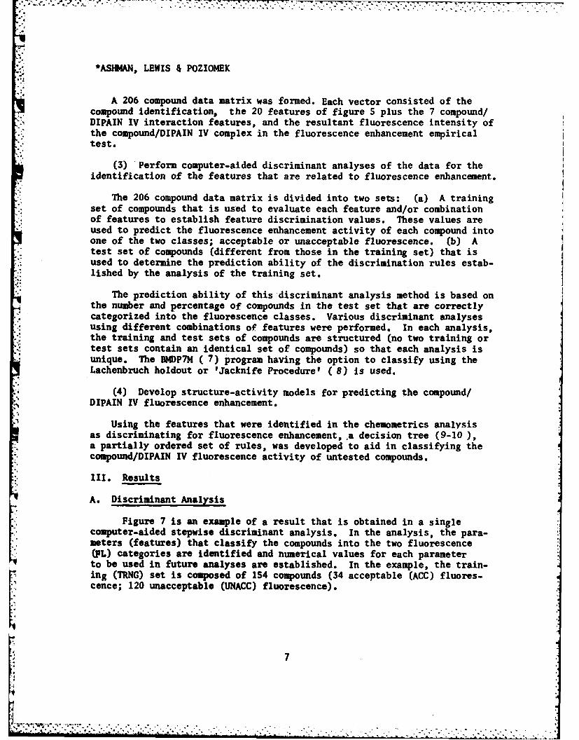
A 206 compound data matrix was formed. Each vector consisted of thecompound identification, the 20 features of figure 5 plus the 7 compound/DIPAIN IV interaction features, and the resultant fluorescence intensity ofthe compound/DIPAIN IV complex in the fluorescence enhancement empiricaltest.
(3) Perform computer-aided discriminant analyses of the data for theidentification of the features that are related to fluorescence enhancement.
The 206 compound data matrix is divided into two sets: (a) A trainingset of compounds that is used to evaluate each feature and/or combinationof features to establish feature discrimination values. These values areused to predict the fluorescence enhancement activity of each compound intoone of the two classes; acceptable or unacceptable fluorescence. (b) Atest set of compounds (different from those in the training set) that isused to determine the prediction ability of the discrimination rules estab-lished by the analysis of the training set.
The prediction ability of this discriminant analysis method is based onthe number and percentage of compounds in the test set that are correctlycategorized into the fluorescence classes. Various discriminant analysesusing different combinations of features were performed. In each analysis,the training and test sets of compounds are structured (no two training ortest sets contain an identical set of compounds) so that each analysis isunique. The BfDP7M ( 7) program having the option to classify using theLachenbruch holdout or 'Jacknife Procedure' (8) is used.
(4) Develop structure-activity models for predicting the compound/DIPAIN IV fluorescence enhancement.
Using the features that were identified in the chemometrics analysisas discriminating for fluorescence enhancement, a decision tree (9-10),a partially ordered set of rules, was developed to aid in classifying thecompound/DIPAIN IV fluorescence activity of untested compounds.
111. Results
A. Discriminant Analysis
Figure 7 is an example of a result that is obtained in a singlecomputer-aided stepwise discriminant analysis. In the analysis, the para-meters (features) that classify the compounds into the two fluorescence(PL) categories are identified and numerical values for each parameterto be used in future analyses are established. In the example, the train-ing (TRNG) set is composed of 1S4 compounds (34 acceptable (ACC) fluores-cence; 120 unacceptable (UNACC) fluorescence).
-- : ""''" "" °"'' ' . ," ' . . , ." . . . . . , . . . - . .. . . -
*ASHAN, LEWIS, POZIOMEK
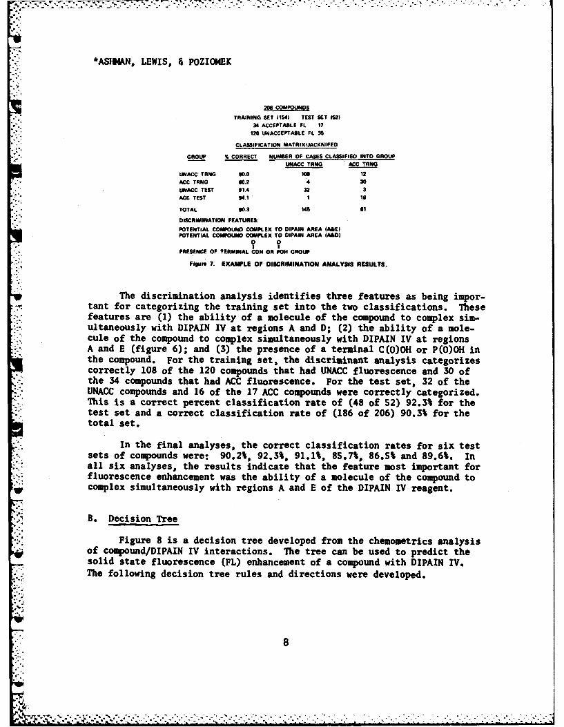
206 COMPOUNDS
TRAINING SET (1541 TEST SET 162)
34 ACCEPTABLE FL 17
120 UNACCEPTABLE FL 35
CLASSIFICATION MATRIX/JACKNIFED
GROUP % CORRECT NUMBER OF CASES CLASSIFIED INTO GROUPUNACC TRNG ACC TRNG
UNACC TRNG 90.0 106 12ACC TANG 80.2 4 30UNACC TEST 91.4 32 3
ACC TEST 94.1 1 16
TOTAL 90.3 145 61
DISCRIMINATION FEATURES:
POTENTIAL COMPOUND COMPLEX TO DIPAIN AREA (ABE)POTENTIAL COMPOUND COMPLEX TO DIPAIN AREA (ABD)
PRESENCE OF TERMINAL CON OR POH GROUP
Figure 7. EXAMPLE OF DISCRIMINATION ANALYSIS RESULTS.
The discrimination analysis identifies three features as being impor-tant for categorizing the training set into the two classifications. Thesefeatures are (1) the ability of a molecule of the compound to complex sim-ultaneously with DIPAIN IV at regions A and D; (2) the ability of a mole-cule of the compound to complex simultaneously with DIPAIN IV at regionsA and E (figure 6); and (3) the presence of a terminal C(O)OH or P(O)OH inthe compound. For the training set, the discriminant analysis categorizescorrectly 108 of the 120 compounds that had UNACC fluorescence and 30 ofthe 34 compounds that had ACC fluorescence. For the test set, 32 of theUNACC compounds and 16 of the 17 ACC compounds were correctly categorized.This is a correct percent classification rate of (48 of 52) 92.3% for thetest set and a correct classification rate of (186 of 206) 90.3% for thetotal set.
In the final analyses, the correct classification rates for six testsets of compounds were: 90.2%., 92.3%, 91.1%, 85.7%P 86.5% and 89.6%. Inall six analyses, the results indicate that the feature most important forfluorescence enhancement was the ability of a molecule of the compound tocomplex simultaneously with regions A and E of the DIPAIN IV reagent.
B. Decision Tree
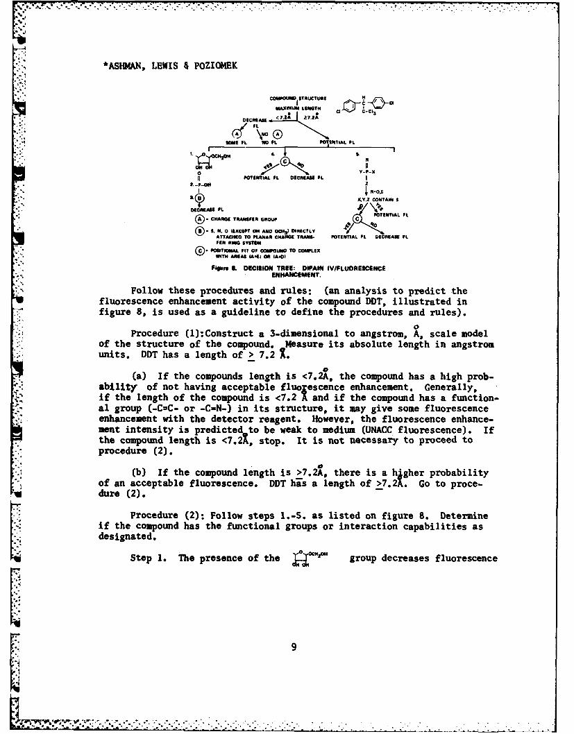
Figure 8 is a decision tree developed from the chemometrics analysisof compound/DIPAIN IV interactions. The tree can be used to predict thesolid state fluorescence (FL) enhancement of a compound with DIPAIN IV.The following decision tree rules and directions were developed.
o.2.
,' , .'. " .., ... ' , ' ., .,' , ." , . ' " ,. . . -" _ . • .. .- ., .. . - .. .. , -, .. " ..,8.
I%,
-- - -.- .". .. .
*ASHMAN, LEWIS POZIOMEK
COMPOUND, STRUCTUREH
MAXIMUM LENGTHOI~cmEI IIA >7, C-cs 3
SOME FL No FL POTENTIAL FL
1. 0S
0 YP-OXUPOTENTIAL FL DECREASE FL I
X.Y.Z CONTAIN S
DECREASE FL 'POTNTA FL,
CHARGE TRANSFER GROUP
__S. N. 0 (EXCEPT ON AND OC"31 DIRECTLYATTACHED TO PLANAR CHARGE TRANS- POTENTIAL FL DECREASE FLFER HING SYSTEM
- POSITIONAL FIT OF COMPOUNO TO COMPLEX
WITH AREAS (A.91 OR fA.O3
Figure B. DECISION TREE: DIPAIN IV/FLUORESCENCEENHANCEMENT.
Follow these procedures and rules: (an analysis to predict thefluorescence enhancement activity of the compound DDT, illustrated infigure 8, is used as a guideline to define the procedures and rules).
0Procedure (1):Construct a 3-dimensional to angstrom, A, scale model
of the structure of the compound. Measure its absolute length in angstromunits. DDT has a length of > 7.2
(a) If the compounds length is <7.2A, the compound has a high prob-ability of not having acceptable fluoescence enhancement. Generally,if the length of the compound is <7.2 A and if the compound has a function-
J , al group (-C=C- or -C-N-) in its structure, it may give some fluorescenceenhancement with the detector reagent. However, the fluorescence enhance-ment intensity is predicted to be weak to medium (UNACC fluorescence). Ifthe compound length is <7.21, stop. It is not necessary to proceed toprocedure (2).
(b) If the compound length is >7.2A, there is a h'gher probabilityof an acceptable fluorescence. DDT has a length of >7.2f. Go to proce-dure (2).
Procedure (2): Follow steps 1.-S. as listed on figure 8. Determineif the compound has the functional groups or interaction capabilities asdesignated.
Step 1. The presence of the 4:H OH group decreases fluorescence
L-.rw9
i

*ASHMAN, LEWIS POZIOMEK
enhancement with DIPAIN IV. This group is highly hydrophilic and can causesteric hindrance when interacting with the DIPAIN IV. If the compound hasthis group, stop (UNACC FL). DDT does not contain this group. Proceed tostep 2.
Step 2. The presence of P(O)OH in the compound decreases the prob-ability of acceptable fluorescence activity. If the compound has thisgroup, stop. DDT does not contain this group. Proceed to step 3.
Step 3. The presence of S, N, or 0 (except OH and OCH3) directlyattached to a planar ring system that has potential for charge transferinteraction decreases activity. If S, N, or 0 is attached to a large planarring system as naphthalene with the substituent on the ring containing anS, N, or 0 directly attached to the ring system, the FL enhancement inten-sity is UNACC. The substituents OH or OCH3 do not have this result. If acompound has this configuration, stop. DDT does not have this configura-tion. Proceed to step 4.
Step 4.(a) If the compound contains a P(O) type configuration.Proceed to step S. DDT does not contain Phosphorus. Proceed to 4(b).
Step 4.(b) The ability of the compound to interact simultaneouslywith regions A plus D or regions A plus E increases the probability of ACCFL. In order to define if a compound interacts with both region A andregion D simultaneously, the following rules are used:
(1) The compound must be able to bind to region A. Region A (figure6) is defined as the diphenyl group region. In order for a compound tocomplex in this area, it must have a lipophilic region (at least a 3 carbonchain) or a -C=C- group in its structure. If a -C(O)O- group is present,there must be at least two carbon methylene groups attached to the -C(0)O-group, (e.g., -C-C-C(O)0-). A compound is positioned to region A by super-imposing its lipophilic or -C=C group on the phenyl ring positioned closestto region D.
(2) Region D (figure 6) consists of the -C(O)-C-C=N-N--C area. Acompound interacting at this region must be planar (usually a phenyl ringor a naphthalene ring configuration). After positioning the compound toregion A, if the compound overlaps on to region D and contains a -C=C-group, it complexes with both region A and D.
(3) Region E consists of the area (figure 6). The
interaction rules used for region A are also used for region E. In order77 for a compound to interact with A plus E, the compound must be able to
bind to A. After positioning it to A, it must have sufficient length to
10
* ,,
Xi' *ASHMA, LEWIS POZIOMEK
overlap on region E. If the compound overlaps on E, an evaluation of thecompound structural components that overlap on E is necessary. If thecompound contains a -C=C- or -C=N- bond that can interact with E by poten-tial charge transfer or a straight chain methylene group that can interactwith E by hydrophobic type interaction, the compound is categorized asbinding to regions A and E. If a compound contains a C(O)OH, P(O)OH,C(O)O-, S(0)0-, or other highly hydrophilic or potential hydrogen bondingregion that overlaps on region E, it is categorized as not binding. Ifthe compound complexes, the result is ACC FL; if it does not, the result isUNACC FL. Stop. DDT can interact with regions A plus E simultaneously.Therefore, DDT is predicted to give a strong flourescence and to be detect-ed by a solid state detection device that uses DIPAIN IV as the detectorreagent.
Step S. This branch of the decision tree is developed for the
- prediction of the detection of I phosphorus, P, compounds(organophesphorous nerve agents and sliulants). The group R of thestructure may be either a sulfur or oxygen atom. In using this part of thedecision tree, orient the compound so that the substituent with the longestabsolute length is positioned at X (figure 8). If X contains a sulfuratom directly attached to the P, it has a high probability of ACC FL. Ifit does not contain sulfur, determine if the structure can simultaneouslybind to region A plus D or region A plus E. If it can interact, theresult is a high probability of ACC FL. Stop.
IV. Discussion
4"I In chemical agent detection, there is a need to develop a detectiondevice that is specific for an agent, and that is reusable, efficient,portable, and simple to use. Solid-state microsensor devices such aspiezoelastic crystals provide a technological advance that may satisfythis need. The DIPAIN reagents studied (1-2 ) and the compound/DIPAIN
, interaction fluorescence enhancement effect have application in coatingsfor these solid-state devices or in the production of a signal that canbe used in solid-state detection.
The objectives of this study were to use chemometrics dicriminantanalysis techniques to: (1) identify the mechanisms related to thefluorescence effects produced; (2) develop compound/DIPAIN IV structure-activity models that can be used as guidelines to predict the fluores-cence enhancement of untested compounds; (3) aid in the design of newsolid-state detection reagents that are specific for a chemical agent.
1711
*ASHAN, LEWIS & POZIOMEK
EXCITED STATE 1w
COMPOUND-11 GROUND STATE -- IIIIIIII
DEACTIVATION1. PREDISSOCTAON
2. INTERNAL/EXTERNAL CONVERSION
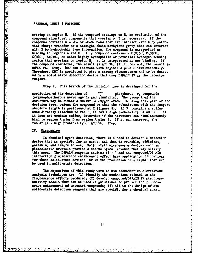
Figuro 9. THEORETICAL RILAtVttS FOR FLUORESEnSCCACTIVITY.
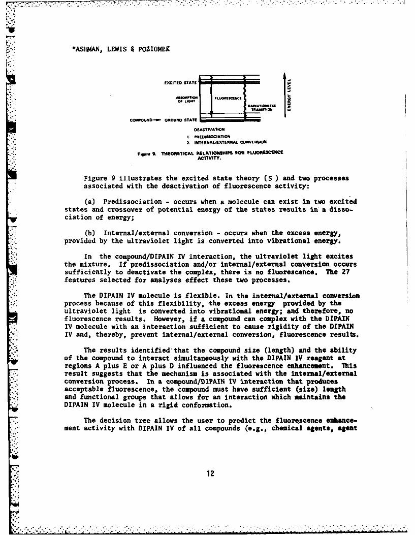
Figure 9 illustrates the excited state theory (S ) and two processesassociated with the deactivation of fluorescence activity:
(a) Predissociation - occurs when a molecule can exist in two excitedstates and crossover of potential energy of the states results in a disso-ciation of energy;
(b) Internal/external conversion - occurs when the excess energy,provided by the ultraviolet light is converted into vibrational energy.
In the compound/DIPAIN IV interaction, the ultraviolet light excitesthe mixture. If predissociation and/or internal/external conversion occurssufficiently to deactivate the complex, there is no fluorescence. The 27
. features selected for analyses effect these two processes.
The DIPAIN IV molecule is flexible. In the internal/external conversionprocess because of this flexibility, the excess energy provided by theultraviolet light is converted into vibrational energy; and therefore, nofluorescence results. However, if a compound can complex with the DIPAINIV molecule with an interaction sufficient to cause rigidity of the DIPAINIV and, thereby, prevent internal/external conversion, fluorescence results.
The results identified that the compound size (length) and the abilityof the compound to interact simultaneously with the DIPAIN IV reagent atregions A plus E or A plus D influenced the fluorescence enhancement. Thisresult suggests that the mechanism is associated with the internal/externalconversion process. In a coupound/DIPAIN IV interaction that producesacceptable fluorescence, the compound must have sufficient (size) lengthand functional groups that allows for an interaction which maintains theDIPAIN IV molecule in a rigid conformation.
The decision tree allows the user to predict the fluorescence enhance-ment activity with DIPAIN IV of all compounds (e.g., chemical agents, agent
12
. ..
. . . . . . . . . . . . . . . . . . . . . . . . . .. . . . . . . . . . . . . . . . . . .

*ASI4AN, LEWIS 4 POZIONEK
simulants, environmental interferences). The decision tree rules can aidin designing or identifying compounds (new agent simulants) that can bedetected by DIPAIN IV. For example, in the design of a simulant for anorganophosphorous agent, it is suggested to take the parent structure
R (R=O,S)IIZ -P- X and to use the decision tree rules to establish the position,
ytype, and functional groups of atoms of the substituents (x, y, z) to beadded to the parent configuration.
In addition to this study, the previous studies (1-2 ) on the DIPAINreagents have established a data base and structure-activity relationshipsthat can be used as guidelines in the design of new solid-state DIPAIN re-agents for use in microsensor devices for the detection of a specific agent.The DIPAIN IV detection is limited to compounds that hive an absolute lengthof >7.2X. Many agents (e.g., GB; absolute length <7.2A) cannot be detectedby the DIPAIN IV molecule. Because the mechanism of enhancing fluorescenceactivity is associated with the ability of the compound to make the DIPAINmolecule rigid, it is suggested to synthesize new DIPAIN reagents havingsubstituents that contain the basic configuration in R (figure 1) as inDIPAIN IV or VI. For this design, either basic configuration of R of IVor VI is designated RR. In order to obtain a reagent that is specific foran agent, the substituent in the RR region should be designed to allow forinteraction with the functional groups or atoms of the agent molecule thatdo not superimpose after positioning the agent molecule to the diphenylregion of the parent DIPAIN configuration. The resultant agent/DIPAINreagent interaction corresponds to the interaction of a compound with theDIPAIN IV molecule at regions A plus E. In the newly designed reagent,region RR is designed as a template to fit the agent.
In conclusion, the decision tree rules and compound/DIPAIN IV inter-action mechanism for predicting solid state molecular association effectsidentified establishes a scientific basis for new concepts and potentialimprovements in chemical detection. The results of this study: (1) allowsfor the design of solid state detection interactions using DIPAIN reagents;(2) provides a set of guidelines for the development of chemical agentsimulants that are detectable using the fluorescence enhancement technique;and (3) provides guidelines for the design of new DIPAIN detector reagentsthat are specific for a chemical agent or simulant. In summary, the DIPAINdata and results have provided fundamental information for chemical detec-tion research which forms a basis for many potential advances in solidstate detection technology.
13
'" " ' " ' "'n''" " - " " ' "n-n-.' . ." :/ 7 - ."
*ASHMAN, LEWIS POZIOMEK(
References:
1. Poziomek, E. J., Crabtree, E. V. and Mackay, R. A. Anal. Let., 13(A14) 1249-1254 (1980).2. Poziomek, E. J., Crabtree, E. V. and Mullin, J. W. Anal. Let., 14
-: (All), 82S-831 (1981).3. Braun, R. A. and Mosher, W. A. J. Am. Chem. Soc., 80, 3048 (1958).4. Mosher, W. A., Bechara, I. S. and Poziomek, E. J. Talanta, 15, 482-484 (1968).S. Joffe, W. H. and Orchin, M. Theory and Applications of UltravioletSpectroscopy. John Wiley & Sons, Inc. (1962).6. Guilbault, G. G., Editor. Fluorescence, Theory, Instrumentation, andPractice. Marcel Dekker, Inc., New York. (1967).7. BMDP-7M, Biomedical Computer Programs P-Series, Univ. of CaliforniaPress. Berkeley, London, Los Angeles. Version Located on Univac 1100,Chemical Systems Laboratory, July 1981.8. Lachenbruch, P., Biometrics, 23, 639, 1967.9. Duda, R. 0. and Hart, P.E. "Pattern Classification and Scene Analysis"John Wiley and Sons, New York, 1973.10. Gane, C. and Sanson, T. Structured Systems Analysis: Tools and
.4 Techniques. McDonnell Douglas Corporation. 1981.
14
o.
.- - -- - - - - - - - - - - - - - - -
- - - - - - - - - - - - - - - - - -
. . . . . ..,. . .
TITLE: A DECISION TREE FOR CHEMICAL DETECTION APPLICATION (U)
The use of trade names in this report does not constitutean official endorsement or approval of the use of such comercialhardware or software. This report may not be cited for purposesof advertisement.
Disclaimer
The findings in this report are not to be construed as an officialDepartment of the Army position unless so designated by other authorized
* documents.
15
%-,.
AYERS, ALLAN, MELVIN, MURFREE, WHARTON, & MARCUCCI
LASER INDUCED POLYMERIZATION REACTIONSIN SOLID PROPELLANT BINDERS (U)
0. E. Ayers, Ph.D., B. D. Allan, Ph.D., W. S. Melvin, Ph.D.,J. A. Murfree, Ph.D., W. W. Wharton, Ph.D., and P. J. Marcucci, 2nd LT
US ARMY MISSILE COMMAND
REDSTONE ARSENAL, AL 35898
INTRODUCTION
The use of organometallic compounds to catalyze urethane reactionsbetween polyols and isocyanates has found extensive use in many industrialand military applications. Organometallic compounds are used as catalystsin the processing of solid propellants to accelerate the curing reactionof the binder in systems where crosslinking involves urethane formationbetween a prepolymer with hydroxyl groups and polyisocyanates.
It has been observed that simple alcohol-isocyanate reactions aresusceptible to photochemical enhancement when exposed to a low intensitytungsten light source (1). This photochemical rate enhancement of urethaneformation occurred in dilute solutions of carbon tetrachloride both inthe presence and absence of organometallic cure catalysts. However, therapid polymerization of polyols with isocyanates requires the presence ofan organometallic catalyst; thus, the concept of photoassisting the re-activity of these catalysts appeared to be an interesting area of investi-gation. Consideration of this phenomenon prompted the idea that a highenergy monochromatic radiation source might be useful in promoting specificchemical reactions and better controlling the cure process of urethanereactions.
This effort examines the effect of ultraviolet and visible laserradiation in conjunction with various organometallic catalysts on theformation of propellant binders. Laser controlled reactions may proceedby pathways not encountered under thermal or other photochemical con-ditions. Also, the laser has the advantage of providing an intensely con-centrated monochromatic beam which allows polymerization to occur atambient temperature rather than at elevated temperatures. The potentialuse of the laser as a Dolymerizatlon tool may provide greater control overthe reaction process.
The work described here was initiated to determine the effects oflaser radiation on the condensation reactions of polyols and isocyanatesand to assess the influence of small concentrations Qf photoabsorbing
17
~~~~~~~~~~- -- - - ---- - - -•. . .. - . . .-. . . .. . .., ..- - - - -... ...................--.... -
AYERS, ALLAN, MELVIN, MURFREE, WHARTON & MARCUCCI
additives. Several classes of organometallic compounds known for theirability to catalyze these types of reactions were screened using ultra-violet lamps. Of these, several compounds were found to be particularly
* receptive to photoactivation in these reactions and were subjected todetailed laser investigation. The results of monochromatic radiation on
7.. these photocatalyzed reactions at 266, 355, and 532 nm are reported here.
EXPERIMENTAL
All experimental samples were prepared by the following procedure:A sample of the organometallic compound was placed in a small mortar andground with a pestle until the material was finely divided. One milli-gram of the organometallic compound was added to 4.25 ml of isophoronediisocyanate (IPDI). The sample was then thoroughly mixed by shaking forone-half hour on a mechanical shaker.
1.41 ml of the IPOlforganometallic mixture was combined with 10 ml ofpolyethyleneglycol adipate (PGA) and thoroughly mixed. The samples werethen evacuated in a glass vacuum desiccator to remove dissolved air andthen opened to the atmosphere. Some samples were run under a nitrogenor oxygen atmosphere. In these cases, the appropriate gas was used toreturn the samples to atmospheric pressure. An aliquot of each samplewas transferred to an ultraviolet 10 mm cell for irradiation. Also analiquot of each sample was used as a reference standard. At various timeintervals, viscosity measurements were made on both the control andirradiated samples. During irradiation, the sample holder was continuouslymoved up and down in a vertical motion by a mechanical device to exposethe entire sample to the laser beam.
All samples that were run in these experiments had an NCO/OH ratioof 1.0 and contained 0.0025 weight percent catalysts. Therefore, to main-tain the same ratio, experimental samples containing hexamethylenedisocyanate (HMDI) were prepareO in a similar manner to those with IPDI.Thus, only 3.3 ml of HMDI were mixed with 1.0 mg of the organometalliccatalyst and then 1.07 ml of this mixture was added to 10 ml of PGApolymer to make the final sample forirradiation.
BLAK-RAY ultraviolet lamps having wavelengths of 254 and 366 nm wereused in the preliminary screening of the organometallic compounds shown inTable I. Those samples which showed increased reactivity were thenselected for laser testing. A Quanta-Ray Model DCR Nd:YAG laser systemwas used as the source of irradiation in these experiments. This DCRNd:YAG laser provided 220 mJ/pulse at 532 nm, 115 mJ/pulse at 355 nm, and50 mJ/pulse at 266 nm. In all the experimental reactions reported in thispaper, the laser was operated at 10 pulses per second.
The Ferranti-Shirley Viscometer System was used to follow the rate ofreaction of the diol prepolymer with the diisocyanate by measuring thechange in viscosity as a function of time.
A Beckman Model ACTA MIV spectrophotometer was used to obtain spectra
18
AYERS, ALLAN, MELVIN, MURFREE, WHARTON & MARCUCCI
of the catalysts listed in Table 1I. The catalysts were used asreceived. Solvents used were spectroquality solvents. The solvent forferrocene was 2,2,4-trimethylpentane. Dibutyltin diacetate solution wasprepared using acetonitrile as solvent. Molar absorbtivities at 266 and,355 nm for ll'-ferrocenedicarboxylic acid were obtained with a methanolsolution, and the molar absorbtivity at 532 nm was obtained in an acetonesolution. The remaining spectra were obtained using methanol as solvent.
The preliminary screening of approximately sixty organometalliccompounds indicated significant photoactivity occurred in about tenpercent of the samples tested. Six samples were selected for closerexaminatidn and controlled exposure to intense monochromatic ultravioletand visible laser irradiation. The results of these experiments are givenin Tables II and V.
RESULTS
These investigations showed that ultraviolet and visible irradiationof catalyzed gumstock mixtures of polyethyleneglycol adipate (PGA) andvarious isocyanates could significantly increase the rates of urethanebond formation. However, the laser enhanced reaction rate was found tooccur only when specific organometallic catalysts were present at thewavelengths used. This secondary acceleration in rate is over and abovethe already increased rate of reaction found to occur with these catalystsunder nonphotolyzed conditions. At the wavelengths investigated thegreatest acceleration occurred when the organometallic compounds containediron. Most other metal containing compounds were found :to produce lesseror no photorate enhancement.
Two ultraviolet lamps were employed to assist in the rapid screeningof a wide variety of candidate organometallic catalysts. One lampproduced low intensity radiation at 254 nm and the other at 366 nm. Theselamps permitted several samples to be simultaneously irradiated. Thepossible effect of photoactivity on the hydroxyl-isocyanate reactions ofPGA, IPDI and various org'nometallic compounds was determined. After aminimum of two hours exposure, the viscosity of each sample was measuredand compared with its appropriate reference sample. Those samples whichshowed the greatest viscosity differences were selected for further inves-tigation with the laser. The results of these initial screening tests areshown in Table I. These viscosity differences between the irradiated andcontrol samples were taken to be a direct measurement of the enhancedpolymerization reaction.
The data presented in Table II show the actual viscosities observe-,as a function of time, when identical PGA and HMDI or IPDI samples con-taining 0.0025% catalyst by weight were irradiated with a pulsed Nd:YAGlaser. The laser enhanced reactions were observed to be extremely sensi-tive to the concentration of catalyst employed. When concentrations ofcatalyst were doubled from the 0.0025% level, the viscosity increased
' - -- 19
A . * . I. * . * .* . .7
AYERS, ALLAN, MELVIN, MURFREE, WHARTON & MARCUCCI
beyond the limit of the viscometer within 30 minutes. Solvents were notemployed to avoid possible complications due to extraneous solvent-assistedcharge transfer complexes which might affect the reaction mechanism.
A cursory examination was made to determine if the reactivity of alinear aliphatic isocyanate (HMDI) differed from that of a cyclicaliphatic isocyanate (IPDI) in these reactions. The data obtained do notshow any reaction enhancement or inhibition trends which could be directlyattributed to a photocatalyzed reaction pathway favoring one isocyanateform over the other.
To reduce possible interferences from the presence of oxygen allsamples were vacuum degassed, returned to atmospheric pressure with air,and sealed prior to irradiation. The only samples observed to undergodetectable color changes contained ferrocene as the catalyst. The faintgreenish appearance was attributed to the formation of the ferroceniumion (1). To determine if the air above the sample had an effect, sampleswere prepared by replacing the air with a pure nitrogen or oxygenatmosphere. Similar rates were obtained with both nitrogen and oxygenalthough they were slightly greater than obtained with air. As minimaleffects were noted with the pure gases, air was used in conducting allother experiments.
Laser irradiation at 266 and 355 nm (Table II) was shown to havesignificant influence on the iron(III) acetylacetonate (FeAA) catalyzedreaction rates. To determine if this increased catalytic influence wascommon to other metal acetylacetonates, a series of these compounds wassubjected to laser irradiation. Representative reaction viscosity datafor the chromium(III), vanadyl(IV), and cobalt(III) acetylacetonatesare shown in Table III and compared with the corresponding iron(III)compound. Little or no photoenhancement on the reaction rate was foundwith these additives and many other similar metal acetylacetonates.Table I shows additional metal acetylacetonates which were subjected to
. ultraviolet lamp irradiation and found to have little or no affect onthese reactions.
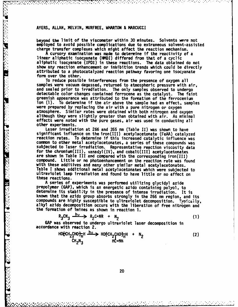
A series of experiments was performed utilizing glycidyl azideprepolymer (GAP), which is an energetic azido containing polyol, todetermine its stabil ;ty in the presence of intense irradiation. It isknown that the azido group absorbs strongly in the 266 nm region, and itscompounds are highly susceptible to ultraviolet decomposition. TyoD'Caly,alkyl azido decomposition occurs with the liberation of free nitrogen andthe formation of imines as shown in reaction 1.
R3CN3 hv z R2C=NR + N2 (1)GAP was observed to undergo ultraviolet laser decomposition in
accordance with reaction 2.
H*H 2CHOnH !IL* HOECH2 HOH + N2 (2)
CH2N3 H =NH
20
2.**7 .
AYERS, ALLAN, MELVIN, MURFREE, WHARTON & MARCUCCI
Copious amounts of nitrogen gas were produced and found entrapped inthe gumstock during irradiation at both 266 nm, and to a lesser extent,at 355 nm. At 532 nm, laser irradiation for up to 1.5 hours did notresult in any noticable decomposition of GAP. No significant photo-
* enhancement was observed to occur at 532 nm in the presence of FeAA.Spectra for the six active organometallic catalysts selected for laser
testing were obtained and molar extinction coefficients (Table IV) werecalculated at 266, 355, and 532 nm.
DISCUSSION
The objective of these investigations was to examine the Influence ofmonochromatic ultraviolet and visible radiation on isocyanate-polyol-organometallic catalyzed reactions to determine if reactive intermediatescould be photoinduced which could affect the mechanism or rate of thesereactions. Various mechanisms have been proposed for these reactions(2, 3).
The absorption of ultraviolet or visible light by a complex may causeone of three effects: (1) the rupture of a bond within the complex, (2)electron transfer between a ligand and the central metal atom, or(3) creation of an electronically excited complex. As previously men-tioned, metal acetylacetonate complexes are reported to form chargetransfer intermediates with isocyanates. It is proposed here that eitherthe formation of the metal-isocyanate complex is facilitated or the com-plex itself is photoactivated by the laser towards attack by the OH groupof the polyol. Although no detailed kinetic or mechanistic studies wereundertaken during the course of this work, the results do agree with thatof others in which an organometallic-isocyanate complex is postulated tobe an intermediate in urethane formation.
The reactions of isocyanates with compounds containing active hydrogenare known to be profoundly influenced by catalytic additives (4). Forexample, it has been speculated that the reaction of an isocyanate with analcohol in the presence of tetravalent tin catalysts occurs through theformation of an intermediate complex between the catalyst and the alcohol.The formation of a donor-acceptor bond between the oxygen of the alcoholand the tin of the catalyst activates the hydrogen on the hydroxyl groupand increases the overall rate of reaction. In this situation, electro-philic attack by hydrogen on the isocyanate nitrogen could result in theformation of a strong hydrogen bond and the subsequent development of thecovalent N-H bond.
Other investigators report the apparent formation of transition metalcharge transfer complexes in polyol-isocyanate complexes (5). The absorp-tion peaks are indicative of d-d electronic transitions within a transi-tion metal ion or of i-- ir* electronic transitions between the isocya-nate and metal ion.
An examination of the summarized results in Table V give conclusivesupport for a laser-induced photoenhancement of metal catalyzed polyol-
: - •21
. 7
AYERS, ALLAN, MELVIN, MURFREE, WHARTON & MARCUCCI
isocyanate reactions. In five of the six samples selected for laserexamination at the three wavelengths shown, it was found thdt the rateenhancements were both wavelength and catalyst dependent. The sixthsample (ferrocene) showed minimal photolytic activity. It is importantto emphasize that two main requirements are needed to achieve photo-enhancement in these reactions. These requirements are: (a) a cataly-tically active ingredient, such as an organometallic compound, and (b)photoactive species. It is apparent from the data (Table V) that nophotoenhancement could be induced in the non-additive containingpolyol-isocyanate reaction. Also, only a limited number of the manyadditives which are known to exert significant chemical catalysis werefound to be additionally photochemically activated at the wavelengthsexamined. The variations in rate can also be seen to be wavelengthdependent (Table V). This wavelength dependence can be attributed tothe relative ability of the complex to enter into a photoactivated orexcited state that is important in the rate determining step.
In the present system, it is reasonable to assume that the mechanismis very similar to that which is operative in the non-photoactivatedreaction. The basis for this assumption is that the photoenhancementeffects are of secondary importance when compared to the enhanced reactionrates obtained by chemical catalyst concentration changes. Laser photo-activation of the intermediate complex provides energy necessary tofurther enhance the catalyzed reaction.
The observation that only a limited number of the approximately sixtymetal complexes tested resulted in enhanced photochemical reactions isattributed to the lack of activation of specific metal-ligand bondt. Thepositive results obtained with FeAA suggested that other acetylacetonatecompounds might also produce similar effects. A series of acetylace-tonates were evaluated with ultraviolet lamps and, in some instances, withthe Nd:YAG laser. The data presented in Tables I and III show thatphotochemical activation was obtained only with iron(III) acetylacetonate.However, wavelengths other than those used in these investigations may-esult in photoactivatlon of metal additives which did not show any signi-ficant rate enhancement.
An interesting observation concerning the three ferrocene derivativeslisted in Table V is apparent from the percent change in viscosities ofthe samples. The photorate enhancement increases are in direct relation tothe increasing order of the electron withdrawing ability of the groupsattached to the ferrocene ring. The order is as shown.
I,l-Ferrocenedicarboxylic Acid > Benzoylferrocene > Ferrocene
CONCLUSIONS
These studies indicate significant enhancement of the polymerizationrate of organometallic catalyzed polyol-isocyanate reactions can be
22
-- . . . . . . . . . . . . . .
7 , .-. .. ,. . . ._:. .. . . . . . . . .,
. . -. . ' - . • . . ., . . o -: - - - - , * - , - , ,
-4
AYERS, ALLAN, MELVIN, MURFREE, WHARTON & MARCUCCI
obtained with a Nd:YAG ultraviolet/visible laser. This enhancement iswavelength and catalyst dependent. While the precise mechanism is notknown, the photorate enhancement appears to be dependent on the formationof an activated metal-isocyanate complex. With the exception ofdibutyltin diacetate, the only additives which gave enhanced photo-chemical activity at 266, 355, and 532 nm were those organometalliccompounds containing iron as the central metal atom. However, not allthe iron compounds screened showed photoenhancement under the conditionsof the experiments. These investigations indicate the laser can be usedto enhance and control urethane formation reaction rates and opens thepossibility that, through proper wavelength selection, other compounds mayact as photocatalysts in-these or other types of reactions.
REFERENCES
(1) S. P. McManus, H. S. Bruner, H. D. Coble, and M. Ortiz, _. Org.
Chem., 42, 1428, (1977).
(2) R. S. Bruenner and A. E. Oberth, J. 2g. Chem., 31, 887 (1966).
(3) D. S. Tarbell, E. C. Mallett, and J. W. Wilson, J. Am. Chem. Soc.,64, 2229 (1942).
(4) K. C. Frisch and L. P. Rumao, Rev. Macromol. Chem., 6, 103 (1971).
(5) T. E. Lipatova, L. A. Bakalo, Y. N. Niselsky, and A. L. Sirotinskaya,J. Macromol. Sc., Chem., 4, ,743 (1970).
.23
23
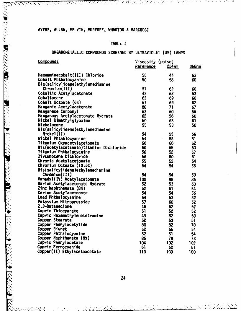
m, 77
AYERS, ALLAN, MELVIN, MURFREE, WHARTON & MARCUCCI
TABLE I
ORGANOMETALLIC COMPOUNDS SCREENED BY ULTRAVIOLET (UV) LAMPS
Compounds Viscosity (poise)Reference 254nm 366nm
Hexamminecobalt(III) Chloride 56 44 63Cobalt Phthalocyanine 50 58 60Bts(salicyltdene)ethylenediamine
Chromium(III) 57 62 60,Cobal ttc Acetyl acetonate 43 62 53
Cobal tocene 62 69 60Cobalt Octoate (6%) 57 69 62Manganic Acetylacetonate 88 71 67Manganese Carbonyl 63 60 56Manganous Acetylacetonate Hydrate 62 56 60Nickel Dimethylglyoxime 60 63 61Nlckelocene 55 53 50Bls(sal icylidene)ethylenediamine
Ntckel(II) 54 55 56Nickel Phthalocyanine 54 55 51Titanium Oxyacetylacetonate 60 60 62Bis(acetylacetanato)titanium Dichloride 60 65 63Titanium Phthalocyanine 56 52 57Zirconocene Dichloride 56 60 61Chromic Acetylacetonate 55 52 54Chromium Octoate (10.5%) 54 54 55Bis(sal icyl idene)ethylenediamtne
Chromium(III) 54 54 50Vanadyl(IV) Acetylacetonate 100 98 85Barium Acetylacetonate Hydrate 52 53 63Zinc Naphthenate (8%) 52 61 54Cerium Acetylacetonate 54 54 56Lead Phthalocyanine 54 53 52Potassium Nitroprusslde 57 60 522,3-Butanedione 45 52 52Cupric Thiocyanate 51 52 52Cupric Hexamethylenetetramine 49 52 50Copper Stearate 52 53 51Copper Phenylacetyllde 80 82 78Copper Biuret 52 55 54Copper Phthalocyanine 52 51 54Copper Naphthenate (8%) 86 78 73Cupric Phenyl acetate 104 102 102Cupric Ferrocyanide 61 62 61Copper(II) Ethylacetoacetate 113 109 100
24.':
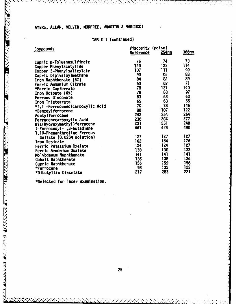
AYERS, ALLAN, MELVIN, MURFREE, WHARTON & MARCUCCIe.
TABLE I (continued)
Compounds Viscosity (poise)Reference 254nm 366nm
Cupric p-Toluenesulfinate 76 74 73Copper Phenylacetylide 120 122 114Copper 3-Phenylsalicylate 107 111 99Cupric Di p1 valoylmethane 93 106 83
• Iron Naphthenate (6%) 84 82 89Ferric Ammonium Citrate 63 62 71*Ferric Cupferrate 78 137 140Iron Octoate (6%) 78 83 97Ferrous Gluconate 63 63 63Iron Tristearate 65 63 65*1,1I.-Ferrocenedicarboxylic Acid 70 78 146
* *Benzoyl ferrocene 88 107 122
Acetylferrocene 242 254 254Ferrocenecarboxylic Acid 236 284 277Bts(Ibidroxy'ethyl)ferrocene 231 251 248
- 1-Ferrocenyl-1,3-butadiene 461 424 4901,10-Phenanthroline Ferrous
Sulfate (0.025M solution) 127 127 127Iron ResInate 162 164 176Ferric Potassium Oxalate 124 124 127Ferric Ammonium Oxalate 138 130 133Molybdenum Naphthenate 141 141 141Cobalt Naphthenate 136 138 136Cupric Naphthenate 156 159 156
A *Ferrocene 98 132 122* *Dibutyltin Diacetate 217 283 221
*Selected for laser examination.
'25
:4 25
!:v :--: ;--- - -,-,,. .. ,...... . .. . . . . . . . *. *... . .* , . .. . .. . . .
AYERS, ALLAN, MELVIN, MURFREE, WHARTON It MARCUJCCI
TABLE 11
I PGA/HMDI(IPDI) CATALYZED BY ORGANOMETALLIC COMPOUNDS
Wavelength Time Viscosity (poise)(nm)- (hours) Control Irradiated
IRON (III)ACETYLACETONATEP532 0.5 110 100
1.5 48 121
266 0.5 122 153
1.0 185 2571.5 427 808
DIBUTYLTIN DIACETATE
532 0.5 116 1041.0 180 1311.5 261 261
355 0.5 81 811.0 981071.5 123 130
266 0.5 114 1151.0 132 1561.5 275 413
26
AYERS, ALLAN, MELVIN, MURFREE, WHARTON & MARCUCCI
TABLE II (continued)
FERROCENE
532 0.5 61 61
1.0 63 61
1.5 52 61
355 0.5 66 74
1.0 69 78
1.5 74 88
266 0.5 60 58-1.0 60 65
2.0 60 81
" BENZOYLFERROCENE
532 0.5 75 811.0 88 1081.5 95 144
2.0 94 162
355 0.5 130 1141.0 239
1.5 -3632.0 283 438
266 0.5 46 522 1.0 66
1.5 892.0 86 1L01
27I!i 27
.-.--7---.-.----.--
-
AYERS, ALLAN, MELVIN, MLJRFREE, WHARTON & MARCUCCI
TABLE 11 (continued)
FERRIC CUPFERRATE
532 0.5 71 871.0 79 1091.5 81 1202.0 99 128
355 0.5 144 2541.0 3521.5 4442.0 208 583266 0.5 55 61
1.0 661.5 842.0 81 98
1 ,1 6-FERROCENEDICARBOXYLICACID
532 0.5 72 871.0 78 1131.5 76 1342.0 75 166
355 0.5 52 431.0 - 61.5 92.0 55 138
266 0.5 40 431.0
-43
1.5 462.0 55 55
28
AYERS, ALLAN, MELVIN, MURFREE, WHARTON & MARCUCCI
TABLE III
EFFECTS OF METAL ACETYLACETONATES ON PGA/HMDIREACTION AT 355 nm
Time Viscosity (poise)Acetylacetonate (Hours) Control Irradiated
Chromium(III) 0.5 54 54:2 -1.0 55 53
1.5 55 56
Vanadyl(IV) 0.5 65 621.0 81 761.5 91 83
Cobalt(III) 0.5 55 551.0 55 561.5 50 62
Iron(III) 0.5 156 1571.0 299 4791.5 484 1021
TABLE IV
* MOLAR EXTINCTION COEFFICIENTS
*COMPOUND 266 nni 355 nm 532 nni
Ferrocene 1.48x10³ 9.50 3.17
Benzoylferrocene 5.65x10³ 6. 69x10 2 1 .88x102
1,1' -Ferrocenedlcarboxyl Ic32
Ac id 6.82x10 3.53x10 0.0
Ferric Acetylacetonate 1.90x10⁴ 2.58x10³ 3.30x10²
Ferric Cupferrate 1.85x10⁴ 3.67x10³ 0.0
Dibutyltin Dlacetate 6.42 0.0 0.0
29
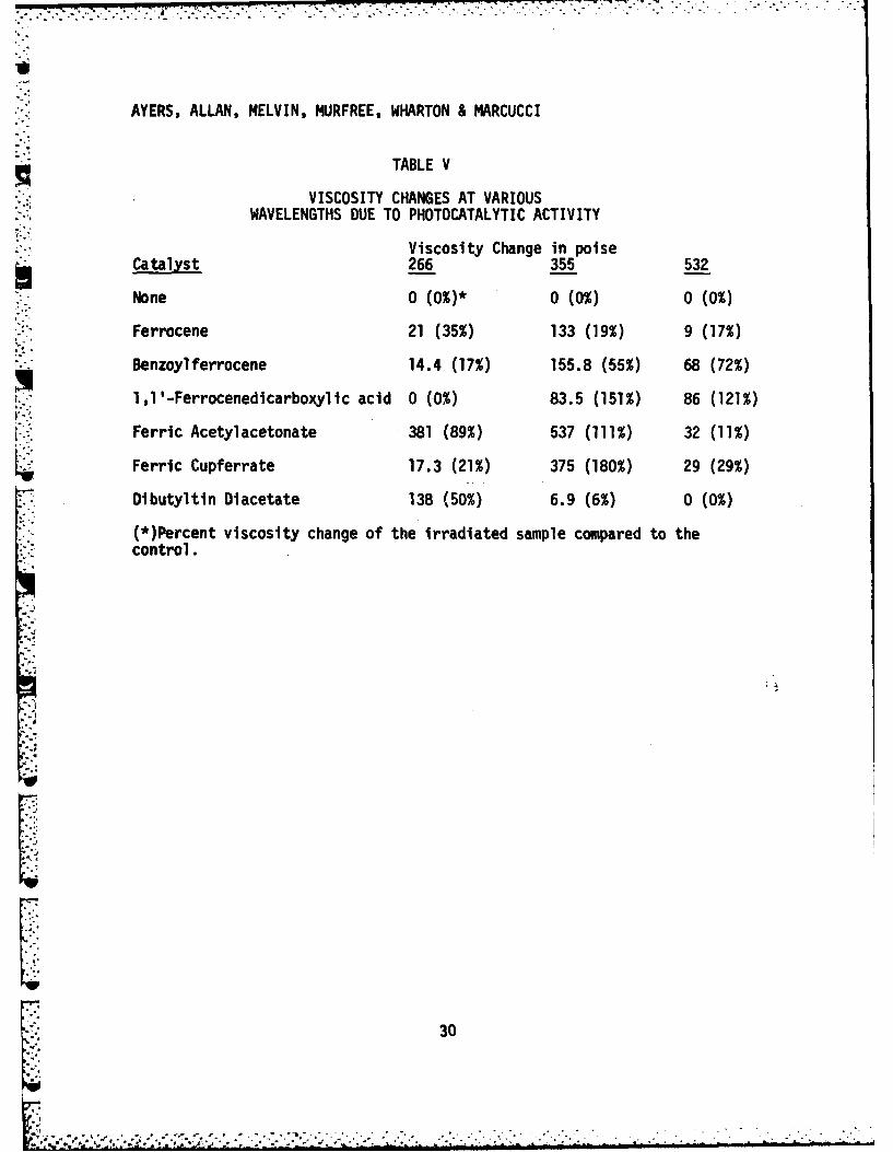
77 7...
AYERS, ALLAN, MELVIN, MURFREE, WHARTON & MARCUCCI
TABLE V
VISCOSITY CHANGES AT VARIOUSWAVELENGTHS DUE TO PHOTOCATALYTIC ACTIVITY
Viscosity Change in poise
Catalyst 266 355 532
None 0 (0%)* 0 (0%) 0 (0%)
Ferrocene 21 (35%) 133 (19%) 9 (17%)
Benzoylferrocene 14.4 (17%) 155.8 (55%) 68 (72%)
1,1'-Ferrocenedicarboxylic acid 0 (.0%) 83.5 (151%) 86 (121%)
Ferric Acetylacetonate 381 (89%) 537 (111%) 32 (11%)
Ferric Cupferrate 17.3 (21%) 375 (180%) 29 (29%)
Dibutyltin Diacetate 138 (50%) 6.9 (6%) 0 (0%)
(*)Percent viscosity change of the irradiated sample compared to thecontrol.
L30
'-" 30
a.! . - - .*.....'- ,' ' *"; ,," "m: , *, ", . 4 .. '.-." " ," . .'. "" """ "-' '" . "'_ - . _- "-" ' : " -" ." - . " ,.-,. ,
BAGBY
THE ENGINEER MODELING STUDY
DR. D. GORDON BAGBYUS ARMY CONSTRUCTION ENGINEERING RESEARCH LABORATORY
CHAMPAIGN, IL 61820
The objective of the Engineer Modeling Study is to measure the contri-bution of combat engineers to the effectiveness of the combined arms team.The research program originated from a Mission Area Analysis (the EngineerFamily of Systems Study (E-FOSS)), which noted that Army war games weregood at representing unit offensive and defensive movements, but weak inmodeling the impact of US and Soviet Union combat engineer activities onbattle outcomes. In 1979, the US Army Engineer School (USAES), represent-ing the Training and Doctrine Command (TRADOC), requested the US ArmyConstruction Engineering Research Laboratory (CERL) to correct this defic-iency. The Engineer Modeling Study was the result.
The Engineer Modeling Study itself is part of the larger Army ModelImprovement Program (AMIP) which seeks to improve the caliber and qualityof Army war games. The three AMIP models shown in Figure 1 interact byfeeding scenarios downward from higher theater-level games to lower leveldivision and battalion-level games and by transmitting combat results up-ward from battalion-level games to theater-level models. The AMIP modelused in the Engineer Modeling Study is the mid-level Corps/Division Evalu-ation Model (CORDIVEM) being developed by the Combined Arms Studies andAnalysis Activity (CASAA). An implicit goal of the Engineer ModelingStudy is accurate and consistent representation of the effectiveness ofengineer effort throughout the AMIP model hierarchy.
Figure 2 illustrates how the Engineer Modeling Study augments theCorps/Division Evaluation Model with an Engineer Module. This modulereceives orders either from the CORDIVEM gamer or indirectly from withinthe game; the module then modifies various CORDIVEM terrain features.These terrain modifications produce three effects: mobility effectsenhancing the movement of friendly ti-aps; survivability effects reducing
* friendly force casualties; and countermobility effects delaying the move-ment of hostile forces.
The Engineer Module is comprised of the three submodules (Figure 3):
31
TI
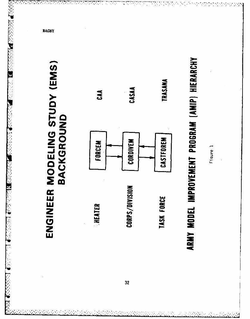
BAGBY
C=
>1. C.3
c,)mW ci C= -4
ac.
(4A LI.
- OmO
Laii MELU C.2z I-- I-nL
321
--------------
S. .E
32. . .
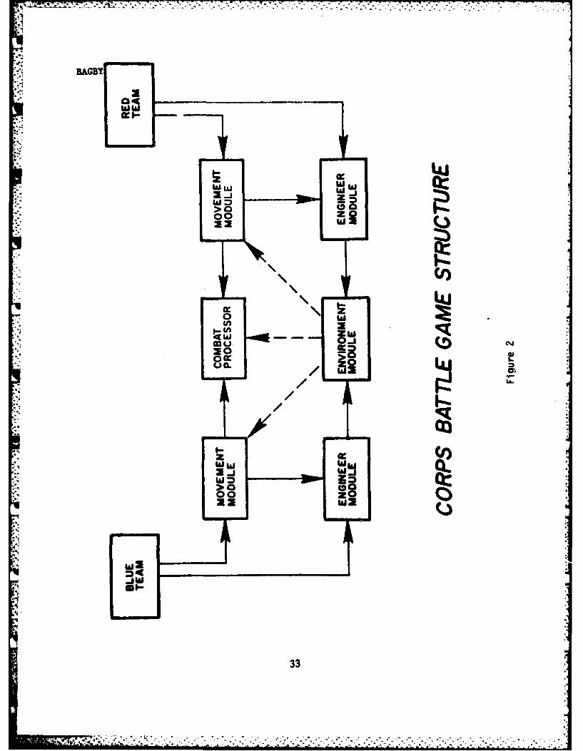
~4; BAGBY
Wai:)
>0 I
ww
>0 %0k
WI 0Zi(4.)
4jj
33
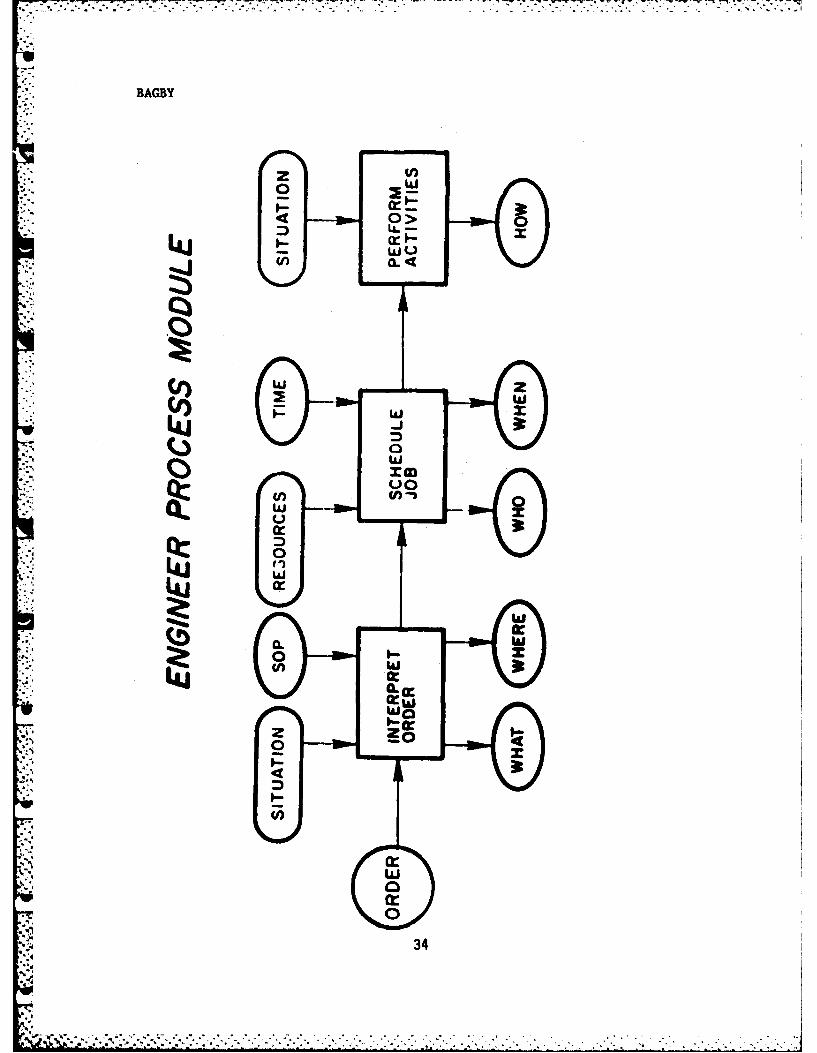
BAGBY
.00
(II)
0
D LL
* 3t
-p 3
0
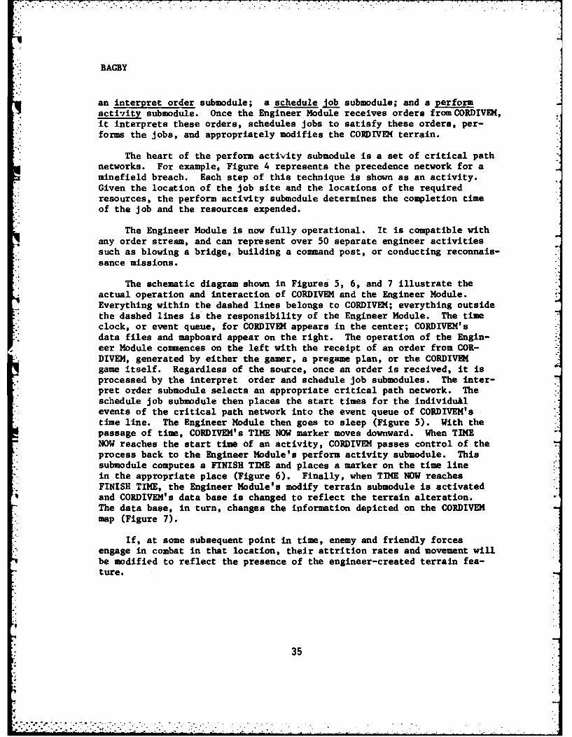
BAGBY
an interpret order submodule; a schedule Job submodule; and a performactivity submodule. Once the Engineer Module receives orders from CORDIVEM,it interprets these orders, schedules jobs to satisfy these orders, per-forms the jobs, and appropriately modifies the CORDIVEM terrain.
The heart of the perform activity submodule is a set of critical pathnetworks. For example, Figure 4 represents the precedence network for aminefield breach. Each step of this technique is shown as an activity.Given the location of the job site and the locations of the requiredresources, the perform activity submodule determines the completion timeof the job and the resources expended.
The Engineer Module is now fully operational. It is compatible withany order stream, and can represent over 50 separate engineer activitiessuch as blowing a bridge, building a command post, or conducting reconnais-sance missions.
The schematic diagram shown in Figures 5, 6, and 7 illustrate theactual operation and interaction of CORDIVEM and the Engineer Module.Everything within the dashed lines belongs to CORDIVEM; everything outsidethe dashed lines is the responsibility of the Engineer Module. The timeclock, or event queue, for CORDIVEM appears in the center; CORDIVEM'sdata files and mapboard appear on the right. The operation of the Engin-eer Module commences on the left with the receipt of an order from COR-DIVEM, generated by either the gamer, a pregame plan, or the CORDIVEMgame itself. Regardless of the source, once an order is received, it isprocessed by the interpret order and schedule job submodules. The inter-pret order submodule selects an appropriate critical path network. Theschedule job submodule then places the start times for the individuAlevents of the critical path network into the event queue of CORDIVEM'stime line. The Engineer Module then goes to sleep (Figure 5). With thepassage of time, CORDIVEM's TIME NOW marker moves downward. When TIMENOW reaches the start time of an activity, CORDIVEM passes control of theprocess back to the Engineer Module's perform activity submodule. Thissubmodule computes a FINISH TIME and places a marker on the time linein the appropriate place (Figure 6). Finally, when TIME NOW reachesFINISH TIME, the Engineer Module's modify terrain submodule is activatedand CORDIVEM's data base is changed to reflect the terrain alteration.
The data base, in turn, changes the information depicted on the CORDIVEM
map (Figure 7).
If, at some subsequent point in time, enemy and friendly forcesengage in combat in that location, their attrition rates and movement willbe modified to reflect the presence of the engineer-created terrain fea-ture.
35
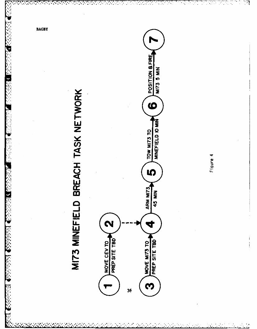
BAGBY
1%
I.U-
o Ton
w I
zLIZ.
9- 0-iI
ILL
ww
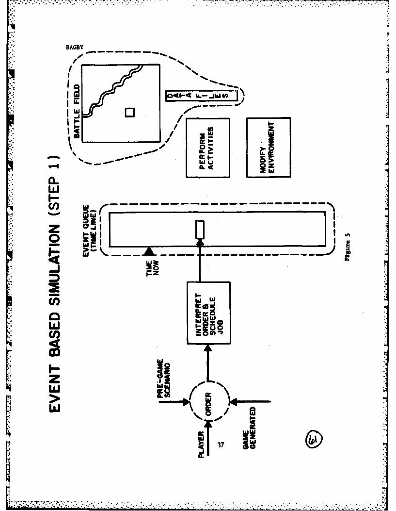
BAGBY
I l041 I-.IU
II'. WI' 0 -*woo
wwI-I --p - ----- - - -
30I
zwo.~E - - - -- - -- --
mmml
go'DLIc
* 37
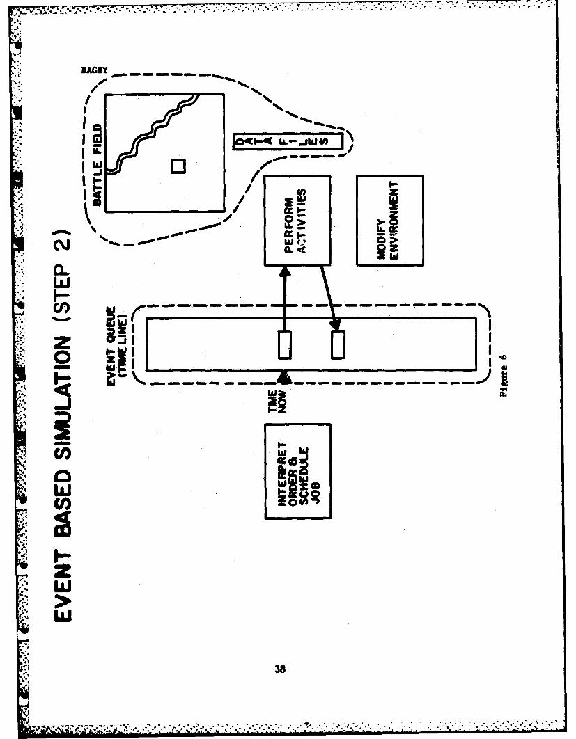
BAGBY__ --
C~l L4%
1w
/
W'r.
ww~w z
zw~~IW
WF'38
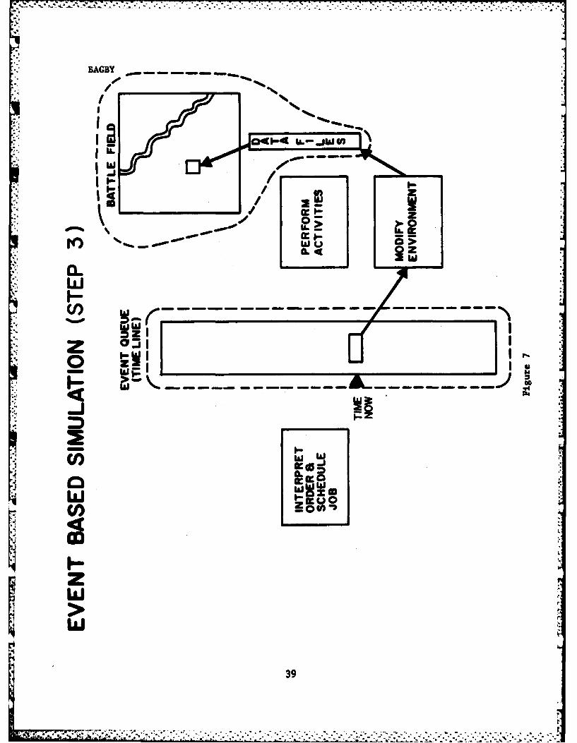
BAGBY ,No .- -Muf
nZI,
a-r
w gCl) - - - - - - - - - - - -
z3
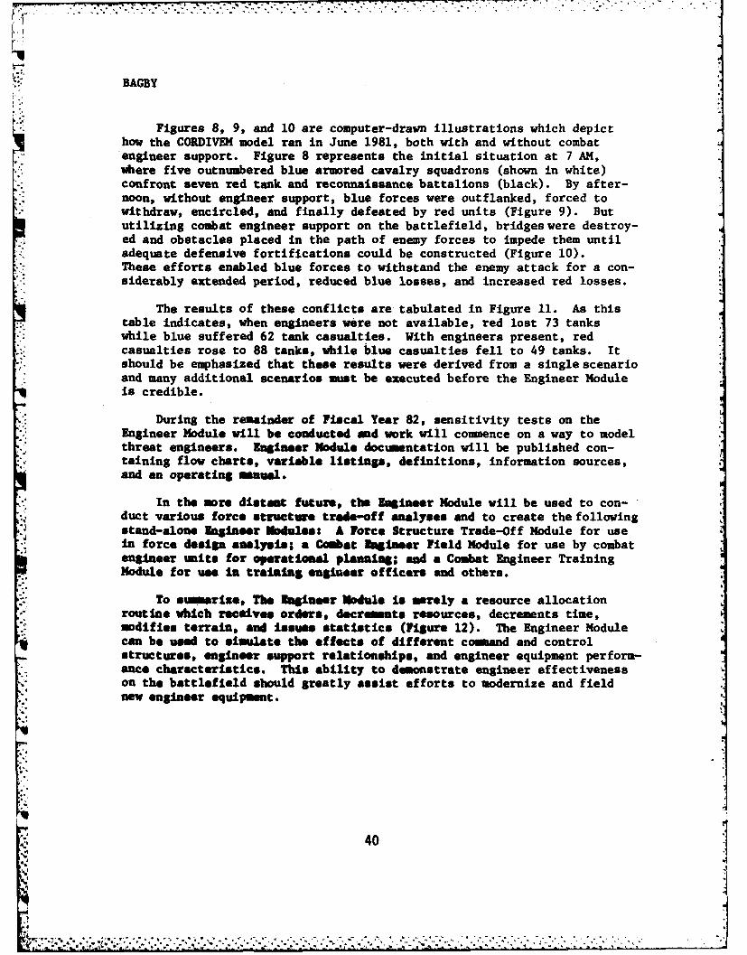
BAGBY
Figures 8, 9, and 10 are computer-drawn illustrations which depicthow the CORDIVEM model ran in June 1981, both with and without combatengineer support. Figure 8 represents the initial situation at 7 AM,where five outnumbered blue armored cavalry squadrons (shown in white)confront seven red tank and reconnaissance battalions (black). By after-noon, without engineer support, blue forces were outflanked, forced towithdraw, encircled, and finally defeated by red units (Figure 9). Bututilizing combat engineer support on the battlefield, bridges were destroy-ed and obstacles placed in the path of enemy forces to impede them untiladequate defensive fortifications could be constructed (Figure 10).These efforts enabled blue forces to withstand the enemy attack for a con-siderably extended period, reduced blue losses, and increased red losses.
The results of these conflicts are tabulated in Figure 11. As thistable indicates, when engineers were not available, red lost 73 tankswhile blue suffered 62 tank casualties. With engineers present, redcasualties rose to 88 tanks, while blue casualties fell to 49 tanks. Itshould be emphasized that these results were derived from a single scenarioand many additional scenarios must be executed before the Engineer Moduleis credible.
During the remainder of Fiscal Year 82, sensitivity tests on theEngineer Module will be conducted and work will commence on a way to modelthreat engineers. Engineer Nodule documentation will be published con-taining flow charts, variable listings, definitions, information sources,and an operating mamal.
In the more distant future, the Engineer Module will be used to con-duct various force structure trade-off analyses and to create the followingstand-alone Engineer Modules: A Force Structure Trade-Off Module for usein force design analysis; a Combat Engineer Field Module for use by combatengineer units for operational planning; and a Combat Engineer TrainingModule for use in training engineer officers and others.
To stmarine, The Ingineer Nodule is srely a resource allocationroutine which receives orders, decrmnts resources, decrements time,modifies terrain, and issues statistics (Figure 12). The Engineer Modulecan be used to simulate the effects of different comand and controlstructures, engineer support relationships, and engineer equipment perform-ance characteristics. This ability to demonstrate engineer effectivenesson the battlefield should greatly assist efforts to modernize and fieldnow engineer equipment.
40
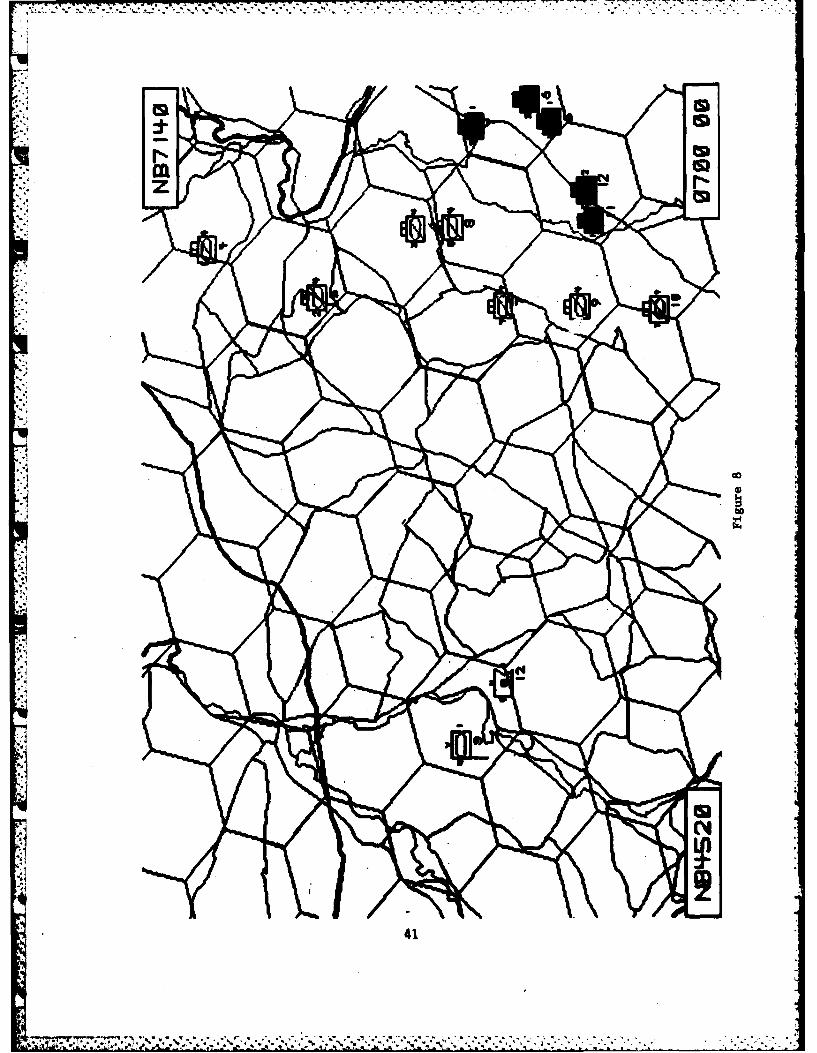
. ... . . . .
to
V14
41

UG
UsI:+
".4
AJA
I42
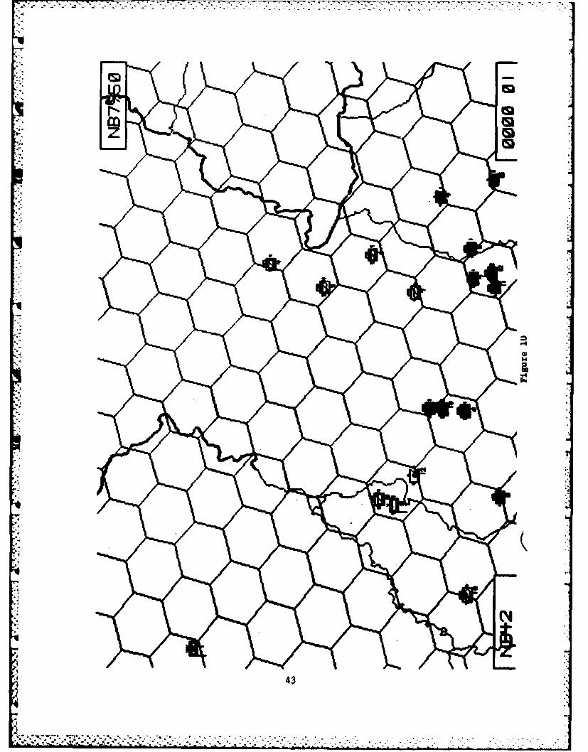
.4p
431
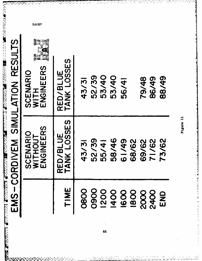
.4I
BAGBY
'U))
w C/)fl~
~cocw
0" ODCL(1
w W Jj v it V~z z N NN N w N% N%0 z~~ r() Cj ) K)-( 0)-rD'O
0 __azI t )0W r% DO
ww
z c .n .*. N. q. ft. %% .
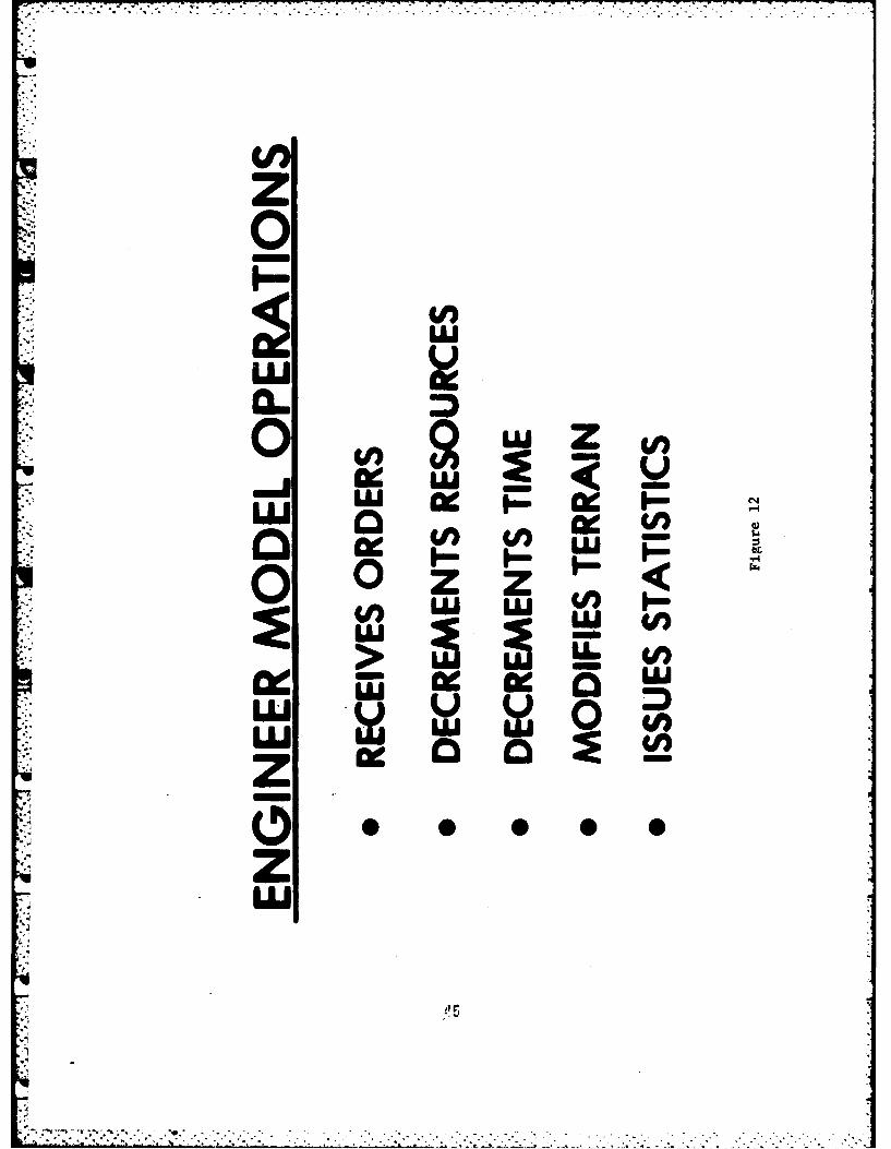
0
og L)ZL
04/ w4/WI
qq% _ wLIwo> LL. V)
0uZ 0 S S
wU
BARR & McKNIGHT
A NEW MIDINFRARED LASER IN HYDROGEN
THOMAS A BARR, Jr., DR.U.S. ARMY MISSILE COMMAND
REDSTONE ARSENAL, AL 35898W. B. McKNIGHT, DR.
UNIVERSITY OF ALABAMA IN HUNTSVILLEHUNTSVILLE, AL 35899
Introduction: The basic research program for high energy lasers (HEL)at the U.S. Army Missile Command has had a major task in the area o* rawlase, concepts for future Army HEL applications. A theoretical ad experi-mental program to explore the possibility for developing a storage laser inhydrogen was carried out during FY 80-82 and resulted In the discovery ofthe laser reported here.
A storage laser is defined as a device which has the ability to storelarge amounts of energy (vibrational or electronic) without largecollisional or radiative losses. There are a number of methods by whichthe stored energy can be extracted as stimulated emission. e.g., (i) bycollisional transfer to another species with a large stimulated opticalcross section, (ii) by an oscillator/amplifier cavity configuration:provided the saturation flux of the storage medium is not too large), oriii) by temporarily increasing the stimulated cross section of the medium
by such means as a field induced dipole.
Nitrogen is a prime example of a storage medium. Energy can be effi-ciently pumped into the vibrational mode of N2 via discharge techniques:the collisional losses are smdll at room temperature and, of course, theradiative cross section for vibration/rotation transitions is zero; andnitrogen can efficiently transfer its vibrational energy to C02.Therefore, the N2/C02 laser is an example of type (I) storage laser.
Practical examples of type (ii) storage lasers are more difficult tofind because they require a value of optical cross section that is largeenough to permit a realizable saturable flux and low enough to prev-ntrap|o losi^of nergy by spontaneous radiation. Optical cross sections of10-- U ci for visible transitions arp required. Examples of thistype of laser are the Group VI lasers - O(IS), S( S), and Se(1S) - whichwere investigated as potential drivers for fusion reactors.
47
BARR & McKNIGHT
The type (iii) storage lasers are, at present, only theoreticalconcepts. In such a laser the storage medium is pumped and, sub-sequently, a significant dipole moment is temporarily created in themolecule by impressing an electric field across the gas. Severalinvestigators have proposed lasers of this type using radiationfields, as from a high intensity pulsed laser (1) or static externalfield from d.c. or low frequency a.c.(2). The problems inaccomplishing this are formidable, and, to date, no demonstration of afield induced laser has been made.
Besides N2, the molecules H2 and D2 are good potential storagemedia. The available electron impact data for H2 indicate that it shouldbe possible to pump into the vibrational mode of H2, D2 and HD via anelectric discharge with a controlled E/N (discharge field strengthper gas density). The vibrational energy transfer kinetics of H2 andD2 have been experimentally measured and indicate that collisional lossesa modest temperatures are small. In principle, the molecular systemencompassing H2, D2, and HD can provide examples of all three types ofstorage lasers: For type (i) we have the H2/HCI and D2/HCl transferelectric discharge lasers (EDL), type (ii) Is provided by HD itself sinceit has a small, permanent dipole moment, and for type (iii) H2, D2, andHD can all be considered for field induced dipole lasers.
Research on HD: Our work started with the analysis of HO as atype(ii), and H2 as a type (iii) storage laser. First order calcula-tions, in which kinetics processes were ignored, showed the conditionsunder which we could expect a sensible gain from either H2 or HD basedon the required partial population inversions. A major job for deve-loping useable external fields would have been required for theH2 laser, therefore, we elected to try the HD laser first.
Requirements for Laser Action in HD: The population distribu-tion for threshold laser oscillation was calculated from a two levelmodel in which the ground vibrational state, with population, Nl, wasthe lower state of the first. vibrational state, with population, Nu,was the upper state. The required inversion density was obtained fromthe solution of the equations:
1. Nu - Nl(2u + 1)/(2J1 + 1) - AN, and 2. Nu + NI z N
Ju and J1 are the rotational quantum numbers. The required inversion*density is M1 - g/s where g is the threshold small signal gain and sis the stimulated emission cross section.
* is used in this text, as commonly done, to represent deuterium.
48
BARR & McKNIGHT
The Einstein A coefficient was derived from data in (3); Doppler linebroadening was assumed based on the physically realizable operatingconditions (press = 4. torr and temp = 770K to 3000K). Also thermalequilibrium was assumed among the rotational states. An estimate ofthe gain per centimeter required for threshold oscillation was made forstate-of-the-art dielectric coated mirrors, R1=.995 for the back mirrorand R2=.98 for the output mirror with no diffraction loss (implies aconcave mirror), and a cavity length of 6.3 mete1r. A sensible outputwai assumed to exist when an absolute gain of 1010 was achieved, i.e.,10u6 photons were produced in a coherent output. Threshold gain is:
3. g = (2L)-l In (RlxR2)'I = (1260.)-1 n (.995x.98)-' = 2.0 x 10⁻⁵ cm-1.
The stimulated emission cross sections, s, were calclated and are:for 770K and 3000K, gspgctively, for ;(11, 6.7x 0- cm and 3.4x10 22
and for P(2) 8.9x10- cm and 4.6xlO-2 cm . Thus the lowest, and presu-mably easiest to get, population inversion is for the P(2) line at 7701K.In this case:
4. N = g/s = 2.0 x 10⁻⁵ cml/(8.9 x 1022cm2) = 2.2x10¹⁶/cm3 .
The total population at 4. tor and 770K i$ 5x10¹⁶/cm3 and the fractionof the gas requl red to be in te upper state to meet the gain thresholdis .04. We assumed, as a working hypothesis based on (4),that we couldobtain sufficient population to overcome mirror losses plus about thesame amount of gaij to build up the laser flux. Under this gain thetime to produce 1016 photons from one initiating photon is:
5. t - ln(N)/(cxa) = ln(10 16/(2x10"5x3x10 10 ) = 60. microsec.,where c is the velocity of light and a is the small signal gain.
The low gain requires that a long path, minimum loss laser beconstructed to provide the best possible chance for laser action in HD.The laser described later in the text resulted from this requirement.h. I includes both a long path length, for maximum gain per "round trip,"and a hemispherical cavity for minimum diffraction losses.
A detailed kinetics computer program was developed concurrentlywith the laser experiment. This program explicitly addressed the calcu-lation of gain in the laser as a function of time for various electricalpumping conditions using a finite-rate kinetics analysis (5). Theresults indicate that small gains are obtainable. However, the magni-.
tude and temporal duration of the gain are not sufficient to meet thegain-time requirements shown in equations, 3 and 5, above. Figure 1.shows the computed maximized gain occurring at 1500. torr (not 4. torras in our experiment) and figure 2. shows that sufficient gain stillfalls short of the minimum time to produce a sensible output. With
49
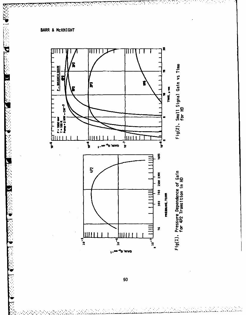
K BARR & McKNIGHT
I,.m
03 ww
In
t-"S
£ W1so
BARR & McKNIGHT
these computational results in hand and having not gotten laser output, experimentally on HO we immediately turned our attention to making a
transfer-storage laser, type (1).
The H?/HCl and D?/HCl Experiments: The laser was then converted, bychange of mirrors, to run as a type (i) H2/HC1 or D2/HCl laser. It wasin this configuration that the presently reported lasers were firstseen. The work on HD showed the sensitivity of the proposed experimentsto gain so that working back through the time and threshold gainproblem we found the conditions under which laser action could bedetected mna fe microseconds. The minimum gain for 1 microsec.generation of 1016 photons is:
6. a = ln(N)/cxt = 36.8/(3xlO1 OxlxlO 6) ='1.2x10 3cm1
Previous work (6) showed that this gain might be achievable. Ourexperiments produced lasers in the midinfrared, first in H2/HCl andlater in D2/HCl, but they were both found to be solely associated withH2 and D2. We stopped work on H2/HC1 and D2/HCl to investigate theselasers. As will be explained later, they are newly discovered electro-nic transition lasers and not storage lasers.
Experiment Design: The experiment (7) is sketched in figure 3.The discharge tube consisted of a 2.5 cm diam Pyrex conical glass pipe.This included two, 3.0 m sections plus end Ts', discharge electrodes,mirror assemblies, and a center 5. cm x 30. cm cross section with anappended cold trap. The cavity output end used a flat sapphire window-mirror, dielectric coated to 95% reflectivity at 3.7 microns. Aconcave Pyrex mirror, 20 m radius of curvature, dielectric coated to99+%, formed the other end. Both mirrors were partially transmittingin the visible, and a He-Ne laser was used for alignment of the cavity.Output was detected on a gold-doped germanium, liquid nitrogen-cooleddetector. Detector voltage, discharge current, and discharge voltagewere recorded on a storage oscilloscope.
The discharge was produced by a Marx bank fired through a resistorand across a gap into the laser tube. The bank consisted of four sta-ges, each a 0.032 microfarads, 125kV, fast discharge capacitor. Normalcharge voltage was in the range between 60 and 75 kV with correspondingerected voltages of 240 to 300 kV. Voltage was measured using a 10:1RC voltage divider with a high voltage oscilloscope probe to provide anoverall attenuation of 10000:1. Discharge current was measured by aninductive current transformer in the ground return circuit.
51
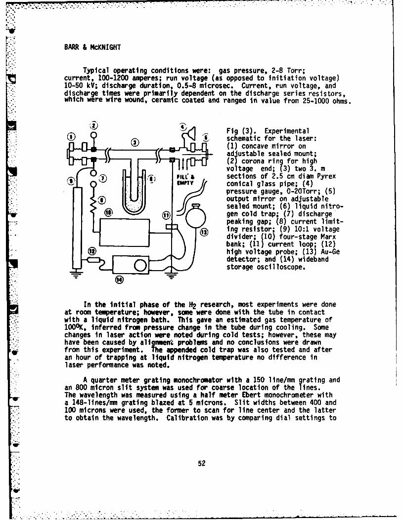
BARR & McKNIGHT
Typical operating conditions were: gas pressure, 2-8 Torr;current, 100-1200 amperes; run voltage (as opposed to initiation voltage)10-50 kV; discharge duration, 0.5-8 microsec. Current, run voltage, anddischarge times were primarily dependent on the discharge series resistors,which were wire wound, ceramic coated and ranged in value from 25-1000 ohms.
4 Fig (3). Experimental
(.) schematic for the laser:(1) concave mirror onadjustable sealed mount;(2) corona rin for high
- voltage end; {3) two 3. m. FIt& sections of 2.5 cm diam PyrexEmY 0,conical glass pipe; (4)
pressure gauge, 0-20Torr; (5)output mirror on adjustablesealed mount; (6) liquid nitro-gen cold trap; (7) dischargepeaking gap; (8) current limit-
3 ing resistor; (9) 10:1 voltage0divider; (10) four-stage Marx
bank; (11) current loop; (12)@high voltage probe; (13) Au-Ge
detector; and (14) widebandstorage oscilloscope.
In the initial phase of the H2 research, most experiments were doneat room temperature; however, some were done with the tube in contactwith a liquid nitrogen bath. This gave an estimated gas temperature of1000K, inferred from pressure change in the tube during cooling. Somechanges in laser action were noted during cold tests; however, these mayhave been caused by alignment problems and no conclusions were drawn
Ir from this experiment. The appended cold trap was also tested and afteran hour of trapping at liquid nitrogen temperature no difference inlaser performance was noted.
A quarter meter grating monochromator with a 150 line/mm grating andan 800 micron slit system was used for coarse location of the lines.The wavelength was measured using a half meter Ebert monochrometer witha 148-lines/m grating blazed at 5 microns. Slit widths between 400 and100 microns were used, the former to scan for line center and the latterto obtain the wavelength. Calibration was by comparing dial settings to
52
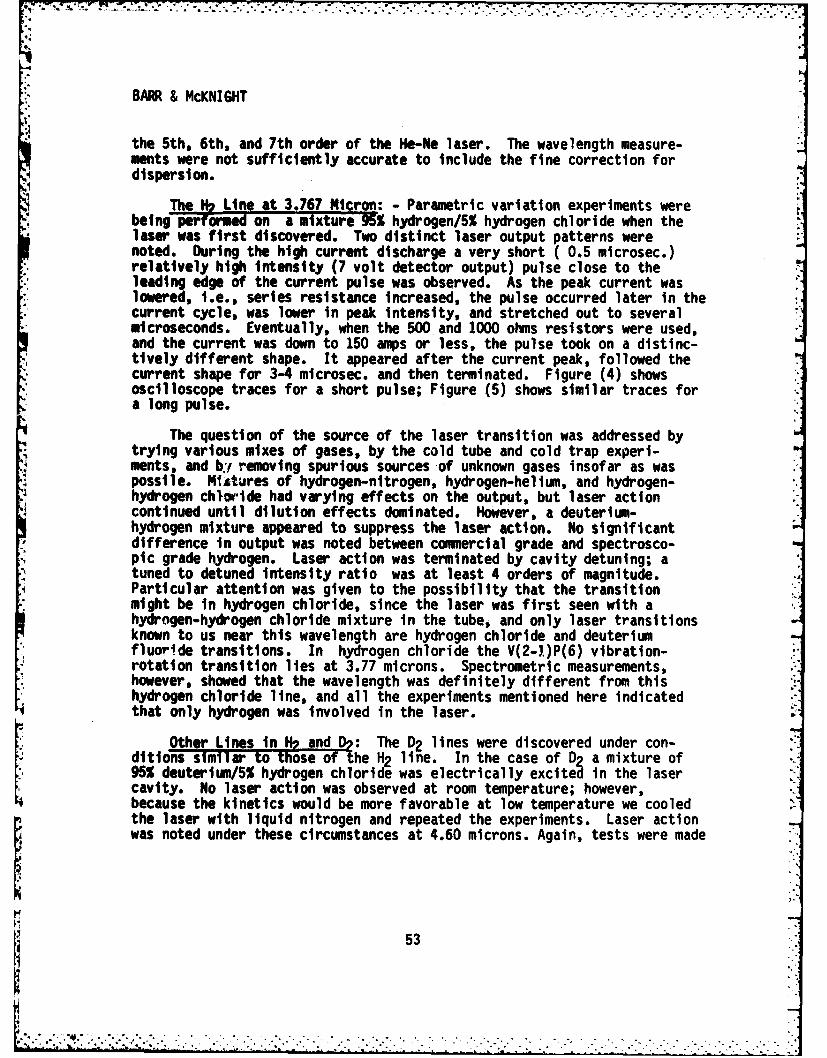
* .4-. ..
BARR & McKNIGHT-'4i
the 5th, 6th, and 7th order of the He-Ne laser. The wavelength measure-ments were not sufficiently accurate to include the fine correction fordispersion.
The I& LtneQat 3.767 Micron: - Parametric variation experiments were
being performed on a mixture 95% hydrogen/5% hydrogen chloride when thelaser was first discovered. Two distinct laser output patterns werenoted. During the high current discharge a very short ( 0.5 microsec.)relatively high intensity (7 volt detector output) pulse close to the
*' leading edge of the current pulse was observed. As the peak current waslowered, i.e., series resistance increased, the pulse occurred later in thecurrent cycle, was lower in peak intensity, and stretched out to severalmicroseconds. Eventually, when the 500 and 1000 ohms resistors were used,and the current was down to 150 amps or less, the pulse took on a distinc-tively different shape. It appeared after the current peak, followed thecurrent shape for 3-4 microsec. and then terminated. Figure (4) showsoscilloscope traces for a short pulse; Figure (5) shows similar traces fora long pulse.
The question of the source of the laser transition was addressed bytrying various mixes of gases, by the cold tube and cold trap experi-ments, and b,,! removing spurious sources of unknown gases insofar as waspossile. Mt.tures of hydrogen-nitrogen, hydrogen-helium, and hydrogen-hydrogen chloride had varying effects on the output, but laser actioncontinued until dilution effects dominated. However, a deuterium-hydrogen mixture appeared to suppress the laser action. No significantdifference in output was noted between commercial grade and spectrosco-pic grade hydrogen. Laser action was terminated by cavity detuning; atuned to detuned intensity ratio was at least 4 orders of magnitude.
4 Particular attention was given to the possibility that the transition'4 might be in hydrogen chloride, since the laser was first seen with a
hydrogen-hydrogen chloride mixture in the tube, and only laser transitionsknown to us near this wavelength are hydrogen chloride and deuteriumfluoride transitions. In hydrogen chloride the V(2-i)P(6) vibration-rotation transition lies at 3.77 microns. Spectrometric measurements,however, showed that the wavelength was definitely different from thishydrogen chloride line, and all the experiments mentioned here indicatedthat only hydrogen was involved in the laser.
Other Lines in H, and D: The D2 lines were discovered under con-ditions similar to those of the H2 line. In the case of D2 a mixture of95% deuterium/5% hydrogen chloride was electrically excited in the lasercavity. No laser action was observed at room temperature; however,because the kinetics would be more favorable at low temperature we cooledthe laser with liquid nitrogen and repeated the experiments. Laser actionwas noted under these circumstances at 4.60 microns. Again, tests were made
53
. . . . .. .. . .. . . . . . . .
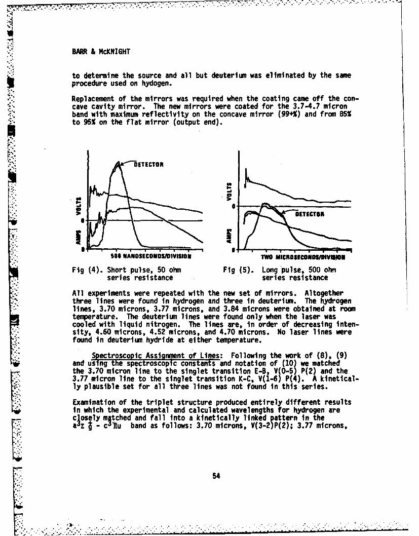
BARR & 1cKNIGHT
to determine the source and all but deuterium was eliminated by the sameprocedure used on hydogen.
Replacement of the mirrors was required when the coating came off the con-cave cavity mirror. The new mirrors were coated for the 3.7-4.7 micron
band with maximum reflectivity on the concave mirror (99+%) and from 85%to 95% on the flat mirror (output end).
r%-a
FI _ __ _ Ig _ _ _ _ _
Im Fig (4). Short pulse, 50 ohm Fig (5). Long pulse, 500 ohwi
series resistance series resistance
All experiments were repeated with the new set of mirrors. Altogetherthree lines were found in hydrogen and three in deuterium. The hydrogenlines, 3.70 microns, 3.77 microns, and 3.84 microns were obtained at roomtemperature. The deuterium lines were found only when the laser wascooled with liquid nitrogen. The lines are, in order of decreasing inten-sity, 4.60 microns, 4.52 microns, and 4.70 microns. No laser lines were
;2 found in deuterium hydride at either temperature.
andSpectroscopic Assignment of Lines: Following the work of (8), (9)and using the spectroscopic constants and notation of (10) we matchedthe 3.70 micron line to the singlet transition E-B, V(0-5) P(2) and the3.77 micron line to the singlet transition K-C, V(1-6) P(4). A kinetical-ly plausible set for all three lines was not found in this series.
Examination of the triplet structure produced entirely different resultsin which the experimental and calculated wavelengths for hydrogen areclosely mtched and fall into a kinetically linked pattern in thea3 z c lu band as follows: 3.70 microns, V(3-2)P(2); 3.77 microns,
54
. ..
i~':.:- 'b-.............I..................-. .~.. - - .--.
BARR &s McKNIGI4T
V(2-1)P(21; 3.84 microns, V(-O)P(2). The set of calculated lines in thisband which fall close to the ones observed in hydrogen are:
TABLE 1. Calculated wavelengths in the a3£;-c3Tu band of H2
microns microns microns
M-0)P 11 3.76 V(2-1)P(1) 3.69 (-Pj 36P 2j 3.93 P(3) 3.85P 3.78
by:
7. Jmax -.59 (T/B)h - .5
Figure 6. shows $he graph of this function fr hydrogen in the a04 statfwhich B a 34.cmA and for deuterium in the cnu state in which B 15.m: Reference (10) tndicat~s that the upper laser level in D)2 may be c 1iu
state tnsted of the state. P(2) appears to be the preferred rota-tional transition for bth gases, which matches the experimental obser-vation that hydrogen produces lasers at 3000K and 1000K. Experimen-tally, we find that the V(2-1) transition in H2, the strongest line,occurs first and is followed in about 0.2 microsec. by the other two lines.This is not unusual in cascading lasers; it is an indication that thelaser action on the main line kinetically produces conditions for theother two lines to appear. Good computational modeling should show thiseffect, too. This delay is shown in the oscillograph traces of Figure 7.
An identical assignment cannot be made for deuterium: first,because its c3Ou state, lies above the a3 Z. state and second, becausethe vibrational and rotational coefficients-(except B) are not known. Inprinciple the laser lines discovered in deuterium could be used to producespectroscopic coefficients. This will be tried at a later date, par-ticularly if additional lines can be found and more accurate wavelenghtsdetermined.
Cavt Properties: The laser cavity composed of a plane outputmirror and a concave back mirror, figure 8, may be considered to be halfof a symmetric resonator. It has an effective mirror diameter of 2.5 cmand a full cavity length of 1260 cm (twice the mirror spacing). A typi-cal wavelength is 4.x?O-4 cm so the Fresnel number is approximately 3.This configuration thus has negligible diffraction loss. The resonatorg parameter is: .
55
. ' ,: :. -A - -....... ';:,,.,.,,, ,,,.,.....-..... ..... . ..- .... •.... ..........-..-. .. ...
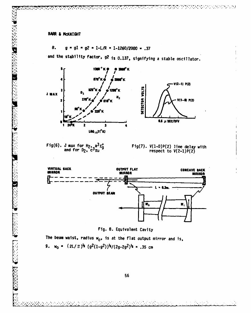
BARR & McKNIGHT
8. g a g1 a g2 1.-L/R .1-12/2000 - .37
and the stability factor, g2 is 0.137, signifying a stable oscillator.
4 6?oK* AWO,/ V(2-I1 P(2)
31, W Ie *w2WKJUMAX 02 / /0
"2 0 1P
S'" A-- p.5. SECIDIVI 240K 2 3 4
LWOGT(0K)
Fig(6). J max for H2, a3z+ Fig(7). V(1-0)P(2) line delay withand for D2 , C3Htu garespect to V(2-1)P(2)
VIRTUAL BACK OUTPUT FLAT CONCAVE SACKIRROR MIRROR MIRROR------ ------------
L. - 6.3.OUTPUT BEAM
Fig. 8. Equivalent Cavity
The beam waist, radius wo, is at the flat output mirror and is,
9. wo * (2L/)hi (g2(1-g2)) 4/(2g-2g2)1 .35 cm
U 56
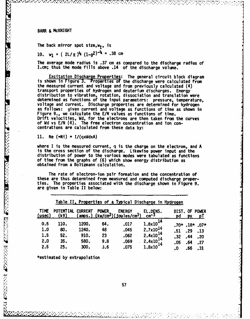
BARR & McKNIGHT
The back mirror spot size,wl, is
10. wI = ( 2L/i )' (1-g2) " = .38 cm
The average mode radius is .37 cm as compared to the discharge radius of1.cm; thus the mode fills above .14 of the discharge volume.
Excitation Discharge Properties: The general circuit block diagramis shown in Figure 3. Properties of the discharge were calculated fromthe measured current and voltage and from previously calculated (4)transport properties of hydrogen and deuterium discharges. Energydistribution to vibration, rotation, dissociation and translation weredetermined as functions of the input parameters: pressure, temperature,voltage and current. Discharge properties are determined for hydrogenas follows: given current and voltage as functions of time as shown inFigure 9., we calculate the E/N values as functions of time.Drift velocities, Wd, for the electrons are then taken from the curvesof Wd vs E/N (4). The free electron concentration and ion con-centrations are calculated from these data by:
11. Ne (-Ni) = I/(qxWdxA)
where I is the measured current, q is the charge on the electron, and Ais the cross section of the discharge. Likewise power input and thedistribution of power to the various modes were tabulated as functionsof time from the graphs of (6) which show energy distribution asobtained from a Boltzmann calculation.
The rate of electron-ion pair formation and the concentration ofthese are thus determined from measured and computed discharge proper-ties. The properties associated with the discharge shown in Figure 9.are given in Table II below:
Table II. Properties of a Typical Discharge in Hydrogen
TIME POTENTIAL CURRENT POWER ENERGY EL.D5NS. DIST. OF POWER(usec) (k) (amps.) (kw/cm3)(Joules/cm 3) cm- pd pv pT
0.5 110. 1200. 64. .017 1.8x10 14 .70* .18* .07*1.0 80. 1240. 48 .045 2.7x10 14 .51 .29 .131.5 52. 910. 23 .062 2.4x10¹⁴ .32 .44 .202 142.0 35. 580. 9.8 .069 2.4x10¹⁴ .05 .64 .272.5 25. 300. 3.6 .075 1.8x10 .0 .66 .31
*estimated by extrapolation
57P.
-. . . . . . . . . .
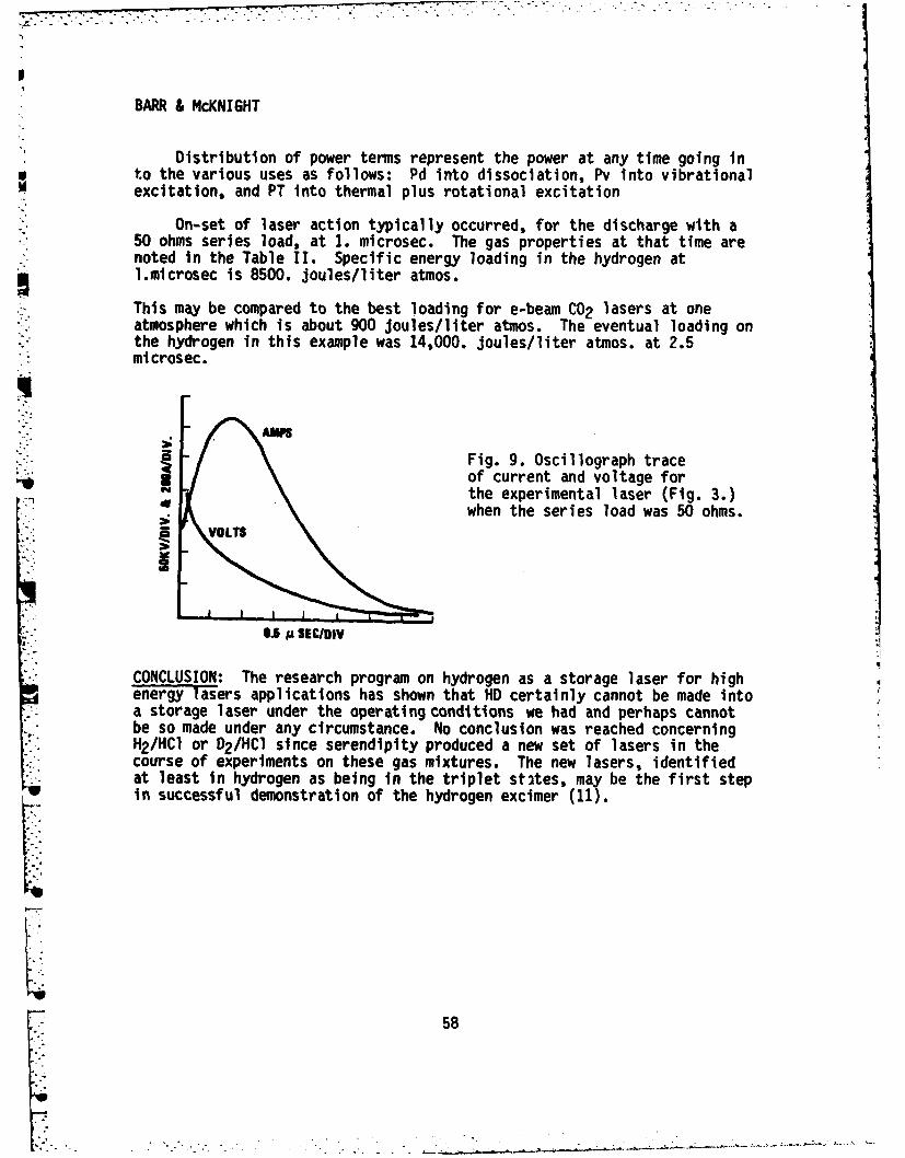
- . - • " . . - . . • - . .
I
BARR & McKNIGHT
Distribution of power terms represent the power at any time going in* to the various uses as follows: Pd into dissociation, Pv into vibrational
excitation, and PT into thermal plus rotational excitation
On-set of laser action typically occurred, for the discharge with a50 ohms series load, at 1. microsec. The gas properties at that time arenoted in the Table II. Specific energy loading in the hydrogen atl.microsec is 8500. joules/liter atmos.
This may be compared to the best loading for e-beam CO2 lasers at one
atmosphere which is about 900 joules/liter atmos. The eventual loading onthe hydrogen in this example was 14,000. joules/liter atmos. at 2.5: microsec.
AM
S Fig. 9. Oscillograph traceU of current and voltage for
the experimental laser (Fig. 3.).5 ewhen the series load was 50 ohms.
* VOLTS
O S SEC/DIV
CONCLUSION: The research program on hydrogen as a storage laser for highenergy lasers applications has shown that HD certainly cannot be made intoa storage laser under the operating conditions we had and perhaps cannotbe so made under any circumstance. No conclusion was reached concerningH2/HCl or D2/HCl since serendipity produced a new set of lasers in thecourse of experiments on these gas mixtures. The new lasers, identifiedat least in hydrogen as being in the triplet states, may be the first stepin successful demonstration of the hydrogen excimer (11).
58
........................................
BARR & McKNIGHT4,
REFERENCES:
1. N. G. Basov, A. N. Oraevskii, and A. F. Suchkov, JETP Lett. 16, 211.(1972)
2. D. W. Howgate, T. G. Roberts, and E. T. Gerry, "New Laser Concepts-Executive Summary Report," TR H-78-2 US Army Missile Command. (Nov 1978)
3. A. R. W. McKellar, Can. J. Phys. 51 389, (1973); Astrophys. J. 185, L
53 (1973); Can. J. Phys. 52, 1144. (174)
4. A. G. Engelhardt and A. V. Phelps, Phys. Rev. 131, 2115. (1963)
5. T. A. Barr, Jr., D. W. Howgate, W. B. McKnight, and R. L. Taylor,'Diatomic Molecules as Storage Media for High Energy Lasers,"
International Conference, Lasers 81, New Orleans. (Dec. 1981)
6. R. Taylor, "Analytical Modeling of Electrically Excited D2/HCI and HClLaser Experiments," PSI TR-58 Final Rpt. on Contr. # N00014-75-C-0035.(July 76)
7. W. B. McKnight and T. A. Barr, Jr., Appl. Opt. 21, No 3. 357-358.(1982)
8. Handbook of Lasers, ed. by R. J. Pressley, 319-322, The ChemicalRubber Company, Cleveland, Ohio. (1971)
9. P. A. Bazhulin, I. N. Kruyazev, and G. G. Petrash, Sov Phys JETP, 20,1068-1069 (1965) and Sov Phys JETP, 21 11-16. (1966)
10. K. P. Huber and G. Herzberg, Molecular Spectra and MolecularStructure, IV, Constants of Diatomic 4olecules, 240-251, 262-267,Van Nostrand Reinhold Company, New York. (1979)
11. C. V. Heer, Phys. Lett. 31A, No. 4, 160-161 (1970)
59
r4
""4" , -,, -,,' -,. . . . . . . :T:I::; I .: J..::. ' -- " ,L .I T, . L ' . .
BAUSSUS VON LUETZOW
Gravity Vector Determination from Inertial and Auxiliary Data andPotential Utilization of Generated Vector Component Information
H. BAUSSUS VON LUETZOW, DR.U.S. Army Engineer Topographic Laboratories
Fort Belvoir, Virginia 22060
1. INTRODUCTION. The present Rapid Geodetic Survey System (RGSS),developed by Litton Systems, Inc. for the U.S. Army Engineer TopographicLaboratories (ETL), has the capability of determining horizontal andvertical positions, deflections of the vertical, and gravity anomalies
U with average rms errors of 1 m, 0.3 m, 2 arcsec, and 2 mgal, respective-ly, for 50 km runs under utilization of post-mission adjustments. Itoperates as a quasi local-level system. It thus does not require alti-tude damping, permits Kalman stochastic error control without greatcomplexity under consideration of observed velocity errors at vehiclestops, and employs effective post-mission adjustments with the aid ofterminal position and gravity vector information only. Present criticalhardware consists of an A-1000 vertical accelerometer, two A-200horizontal accelerometers, and two G-300 gyroscopes. Although data
:- i utilization from repeated runs has resulted in average deflection rms
errors of about 1 arcsec, the requirement of a maximum rms error of 0.5arcsec necessitates the incorporation of higher performance gyroscopesand accelerometers. Thts would simultaneously achieve conventionalsurveying accuracy (10-7). Following the approximate elimination of theeffects of constant gyro biases on positions under utilization ofaccurate initial and terminal coordinates, the remaining dominant errorsource is gyro correlated random noise. In this respect, the pertinent Ipartpeters for the G-300 instruments are a standard deviation of 0.0020hr- and a correlation time of 3 hours. Another error source to b.e 4considered is the accelerometer scale factor, assumed to be constant fora test run. The standard scale factor error for the A-200 accelerometeris 0.01%. Correlated accelerometer noise is characterized by a standarddeviation of 10 mgal and a correlation time of 40 minutes. Both corre-lated gyro random drift and correlated accelerometer measurement errorsaffect the accuracy of deflections of the vertical estimated frominertial data and initial and terminal deflection components, possiblyaugmented by corresponding geodetic azimuths. In order to achieve
61-a
BAUSSUS VON LUETZOW
deflection accuracies smaller than or equal to 0.5 arcesec rms, it is,therefore, necessary to install higher performance gyros and accelero-meters. A significant reduction of the two autocorrelation parametersis also a necessary prerequisite for the optimal statistical estimationof deflections of the vertical. The Litton 0-1200 gyro is expected tobe compatible with the stringent defle tion accuracy requirement. Itsrandom drift error is about 0.0010 hr- and its autocorrelation parame-ter is short. For details, reference is made to Litton [1] and Huddle[2]. The A-100 accelerometer addressed by Litton [3,4] has a standardscale factor error of approximately 0.005%. Correlated accelerometernoise is 2 mgal rms, equivalent to about 0.35 arceec.
2. DETERMINATION OF VERTICAL GRAVITY COMPONENT. In a local Cartesiancoordinate system tangent to a normal gravity surface, with x as west-east coordinate, y as south-north coordinate and z as vertical coordi-nate, positive upward, it is
g (g , -g, -g) (i)
In eq. (i), g is the gravity vector at the origin, -g is its verticalcomponent, and gn and -gE are its horizontal components, n and E beingthe prime and meridian deflections, respectively. For computationaland estimation purposes it is advantageous to use the gravity anomaly Agg -y with y as normal gravity, to be found by consideration of the
elevation above the normal reference surface.
The RGSS error differential equation for the vertical channel,including first and second order time derivatives, is
-2w z - (PN +2aN) PU +Ag+a + A 6 - A 6 (2)a N N-s x ix y Zy
where the symbol 6 ?f position errors 6x, 6y, 8s is omitted for simplic-ity. In eq. (2), we - g R - with R as the earth's mean radius is thesquared Schuler frequency, PN - VXR 1 with Vx as the system's eastvelocity is the north angular rate, ON is the north earth rate, pE -
-VR'" with V as the system's north velocity is the east angular rate,a5 s the vertical accelerometer error, Ax and A7 are east and northaccelerometer outputs, and 6 and 8yg are z-axis misalignment errgrs inthe x,s and y,z plages. At the system a stop, the term involving x maybe estimated since x is observed, and the last two.terms are omitted.At terrestrial vehicle speeds, the term involving y becomesinsignificant.
I. See Litton 15J, p. 3-132.
62
BAUSSUS VON LUETZOW
Because of initial calibration ;(to ) 0 = 0 and zo= to= t Axo
SAY.wc, e 0, the term Ag + az has to be subtracted from s(tv) = z," Atsurvey vehicle stop, therehre, under omission of PNt and pEt in eq.
(2),2
Ag -Ag o + % + lN V- 2% % -(a - a 3 ), (3)V 0
:i I where the error terms 2ws2Zv and az - are weakly correlated. If z
and a z are considered as random variables with zero means and estimatedvariances and covariances, respectively, the gravity anomaly errorvariance is
var 8g, 4w, varz + var (az -az (4)V 0
Since zv has an average rmg error of 0.3 m due to Kalman filter estima-tion by means of observed zv at vehicle stops and a post-mission adjust-ment under utilization of a terminal ze, the rms error induced by zv isonly 0.1 mgal. High accuracy determinations of gravity anomalies or ofthe vertical component of gravity by means of a local-level inertialsystem thus require a high performance vertical accelerometer, highaccuracy height determinations and, possibly, utilization of t-observa-
tions at vehicle stops.
The availability of Age and ze at the end of the survey permits theSdetermination of f in eq. (3). Empirical corrections for
a3 - a in the formV 0
C C(a -a ) Cf (5) (a,.
e 0
prevent error growths to about 2 var a .* Under restrictive assumptions,with the omission of the subscript s,
cov (aV - a, a. - . [var (a a (6)
3. SINLI NORIZOWTAL CHAMNEL DETERINATION OF DEFLECTIONS OF THEvurI VL. While the determination of gravity anomalies may he lessrapily aooomplished with high accuracy by mans of gravimeyer andheight msaremoents, astrogeodetic and gravimetric determinations of
63
IF
BAUSSUS VON LUETZOW
deflections of the vertical are time-consuming. According to Moritz[6]. astrogeodetic and gravimetric rms errors are approximately 0.2arcesec and 1.5 arcsec, respectively. Rapid inertial-astronomicdeterminations of n and C with rms errors not exceeding 0.35 arcesecwould thus be highly economical and satisfactory for many purposes.Both the single and coupled horizontal channel determinations of n and Crequire the utilization of the simplified error differential equations2 :
* ONz N~ + a E(7
*-g*-.+ +aN (8)
1 z " -ltr'i + R- 1 (N N sec #)y -EN wN#E + (9)
i m -1 "
NI R + mEz ~ z#E +0 (10)
Symbols used in the foregoing equations including total time derivativesof first and second order are, except for those defined in section 2,
#z azimuth platform attitude error
+N platform tilt error about north axisplatform tilt error about east axis
SE east acceleration of survey vehicleSN north acceleration of survey vehicleaB correlated east accelerometer erroraN correlated north accelerometer error# geographi? latitudeI Wz - Oz + R- tn 0s Vx vertical at rate
:WN a AIN - + ve north spatial rate•WE W -R-1V 7east spatial ratea azimuth-axis angular drift rate error
V: 0 north axis angular drift rate erroreast axis angular drift rate error
?or land vehicles, eqs. (9) - (11) my be simplified by omission of pN,
2. A more complex systom my be required. geo Litton [5], pp. 3-252 -3-254.
64
Ki - BAUSSUS VON LUETZOW Iov, and ps R tn#.V,, and by use of constant accelerations SN and SEwhich should be approyimately achieved. Then, wz = Osin# and wN -0co8#
* where 0 denotes the earth's inertial angular velocity. The initialconditions at t - 0 are, unler congideration of plumbline leveling, wz(O)-0, *,(o) -o, Tic o0 - o x(o) - y(o) - x(o) - y(o) -O.
In the general ROSS mode of operation, position and gravity vectorinformation is generated. The Kalman filter mechanization is simplifiedby setting wEON - w 0 in eqs. (9) - (11) which results in the
, uncoupling of the horizontal channel differential equations. This isnot critical in the context of present instrumentation for travelperiods of 2 hours. As an example, eqs. (8) and (10) may then be formu-lated at the end of the first travel period, whence t -t ,
Yl 4 1 - l a 1 - aN (12)0
# 1 " " R -Y f o y d t + 1
0t1
In eq. (12), accelerometer calibration at to= 0 has been taken intoaccount. The quantity.-R y in eq. (13) is well estimated by the ob-served velocity error y. After implementation of the corresponding tiltcorrection, under neglect of insignificant estimation errors and consid-eration of the bias error fE(ti),
Y(ti) i "4E - g (Ci to + gfi f T -( ) dt + N aN (14)0 0
. . tY(tn);n gE " (En - gfn( dt a N - (15) In 0 n 0
The propagation of constant gyro blas.errors may be approximated bya solution of eqs. (9) - (i) with y - w, 0 and by treating Wand wZ as constants in accordance with Huddle The result is J
E + csz ;t - /2) (l6)
41, at( ftSoz/2 + I (7
a; t t%/2 ) (18)
Uner considertion of termial deflection and asinuth errorn at t -t
. L6
BAUSSUS VON LUETZOW
it is possible to estimate 5, , V from
nIN " In (19)' ". An
L J"t U Jestmted observedn
Equations (15) and (16) show that the computation of fiin eq. (14) isto the first order associated with an error i
ti t6 0E tn [gfo (y- )dt + a - a] (20)
tn n 0
The final solution for the meridan deflection of the vertical from eqs.(14) and (20) is a a a. a
N N a1 a t a - aW0 i E . t n " (21)
.fti t. t
" f (-f - j)dt -ti n (y . )dtn
Equation (21) may be supplemented by
8ti ti6 1i" 0 t( e6o) -r *~) (22) in ~ n
to account for astrogeodetic deflection errors and accelerometer biase~rors. For a straight traverse, the last term in eq. (22) tends tocancel out.
The rms deflection error CE(ti) can be computed by covariance analysisinvolving the terms without parentheses in eq. (21). Under inclusion ofthe first two terms of eq. (22),
=var + var + var y - var o + ( T a) rn ' (23)n n
where var a is the accelerometer-induced variance and var yidesignatesthe gyro-induced variance. Under consideration of present RSS param-stere, identified in section 1, the rms deflection error o is approxi-mately presented in Figure I for a vehicle speed of 30 kmits
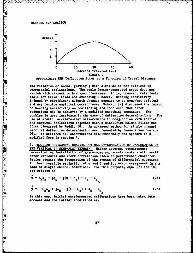
-. .. .
BAUSSUS VON LUETZOW
arcsec3
2
0 15 30 45 60Distance Traveled (km)
Figure 1Approximate PNS Deflection Error as a Function of Travel Distance
The variation of normal gravity g with altitude is not critical interrestrial applications. The scale factor-generated error does notvanish with respect to L-shaped traverses. It is, however, relativelysmall for travel times not exceeding 2 hours. Heading sensitivity
" induced by significant asimuth changes appears to be somewhat criticaland may require empirical corrections. Schwarz [7] discussed the impactof heading sensitivity on positioning and concluded that error
. reductions may be achieved by a modified smoothing procedure. Theproblem is more intricate in the case of deflection determinations. Theuse of static accelerometer measurements in conjunction with initialand terminal deflections together with a simplified Kalman filter wasfirst discussed by Huddle [8]. An advanced method for single channelvertical deflection determination was presented by Baussus von Luetzow[9]. It utilizes all observations simultaneously and appears in amodified form in section 4.
4. COUPLED HORIZONTAL CHANNEL OPTIMAL DETERMINATION OF DEFLECTIONS OFTHE VERTICAL I' SEMI-FLAT TERRAIN. Higher accuracy requirementsnecessitating installation of gryoscopes and accelerometers with smallerror variances and short correlation times as performance character-istics require the integration of the system of differential equationsfor best possible estimation of n and F and for error assessment in thecase of single channel solutions. For this purpose, eqs. (7) and (8)are written as
x - SN~z - 8*N + g(T - no ) + aE - aE (24)0
y- -S 1 + g# - g( - o ) + a N - a (25)
0In this way, initial accelerometer calibrations have been taken intoaccount and the initial conditions are
67
BAUSSUS VON LUETZOW
E(o) - N (o) " *(0) - i(o) f (o) X(o) - y(o) 0 (26)
The accelerations SN and SS can probably be neglected. If the system istreated as one with constant coefficients as a good approximation, aclosed solution as a function of time is possible. Because of intermit-tent Kalman filter corrections and the need for numerical weight factorsit appears to be advantageous to attempt a numerical solution for x andy under utilization of terminal deflection and azimuth data. For eco-nomic reasons it is assumed that the survey vehicle travels approxi-mately at a constant speed when in motion and stops every 3 minutes for1 minute. The speed should not exceed 10 msec in order to restrict thelength of travel intervals.
Solutions for fE, *N,*z, x, y, x, y are obtained in accordance withthe integration schemes
F - 0 + F At (27)
: " 21P i " v-2 (At) 7 -i (28)
with At - 30 sec and possibly 60 sec. The solution structure at the endof the first stop interval, indicated by the subscript s-1, is
V V V V V
F V I % vv + b wv + c + (29)
In eq. (29), v - g (n - no ) + aE - aEe, w -g( - to) + aN aN.
Under consideration of Kalman filter tilt corrections, assumed forsimplicity to eliminate the integrated first two terms in eq. (9) andthe first term in both eq. (10) and (11),
(2) V V V V V.:.: A vv + B wv + Cv % x + O v ( 0V1 - VA+ Bw ~ v .XD v+yv + T, (30)
where T1 and subsequent T. represents an aggregate of tilt-inducedrandoip errors. During the stop interval, eqs. (9)-(11) are integratedwith x - y - y - 0 with a resultant effect on eqs. (7) and (8). Theintegration is then continued and yields under utilisation of averagebiases the solution structure
.. ... .
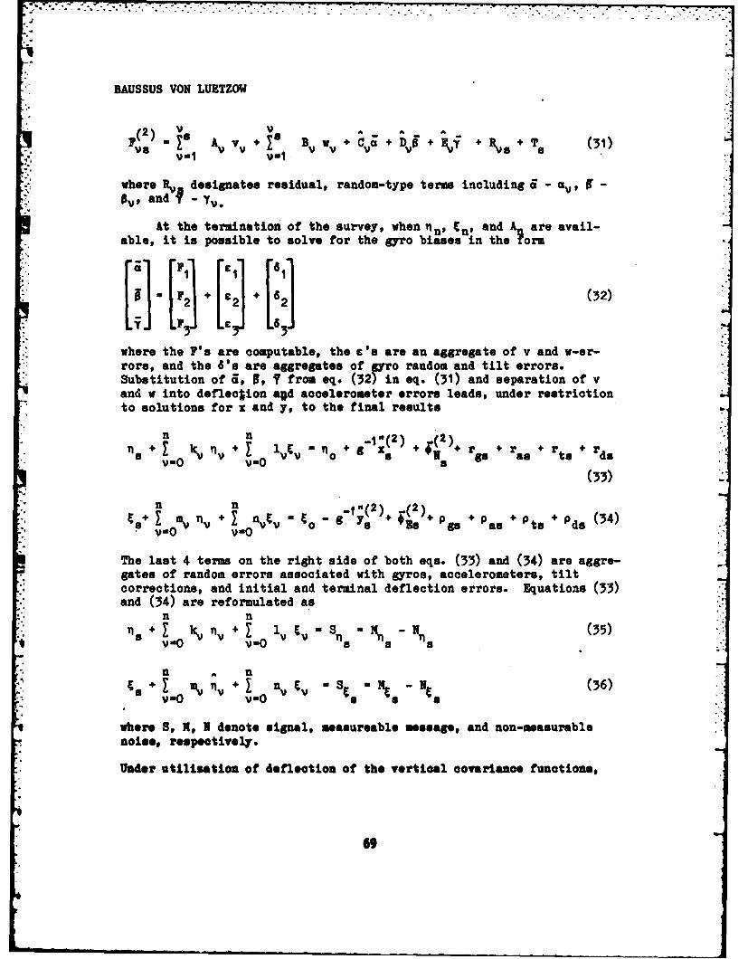
BAUSSUS VON LUETZOW
v(2 A v + BV wV + D E" j + AV TS
v -. , V= *1
where %L_ designates residual, random-type terms including -i, 1, I -
,v , and -Y.
At the termination of the survey, wheninn, g and A, are avail-able, it in possible to solve for the gyro biases in the form
F] [2 [ J + [82 (32)
Le.
where the I's are computable, the O's are an aggregate of v and w-er-rors, and the 8's are aggregates of 0ro random and tilt errors.Substitution of i, 0, I from eq. (32) in eq. (31) and separation of vand w into deflection agd accelerometer errors leads, under restrictionto solutions for x and y, to the final results
T1S+ 1 + . ,v no. +g+ gs a t, dv=O v=O v *I+ r r +
(33)
n n ..1"'(2) _.(2)C + I nvt o -g ys + + P s +s + ts do (34).,. 0 = V + Y. % V6 B o as tos P al
The last 4 terms on the right side of both eqs. (33) and (34) are aggre-gates of random errors associated with gyros, accelerometers, tiltcorrections, and initial and terminal deflection errors. Equations (33)and (34) are reformulated as
n n.in, + kv n v + 1 V tv " T11 "n N, - (35);V .0 v.- 0 a a 8 -N
n nvg O vO v S -N (36)
where S, N, I denote signal, measureable message, and non-measurablenoise, respectively.
Under utilisation of deflection of the vertical covariance function.,
69
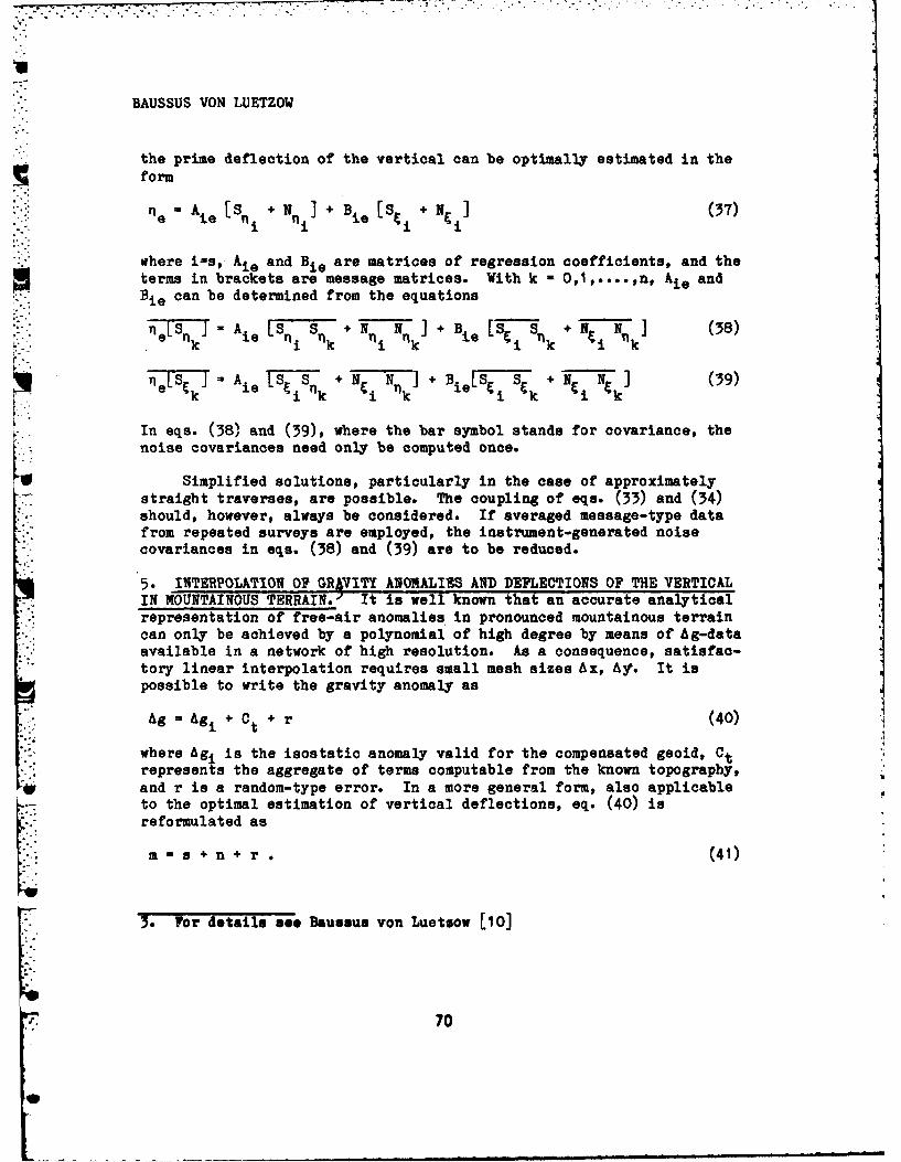
BAUSSUS VON LUETZOW
the prime deflection of the vertical can be optimally estimated in theform
ne = Ae [S + N +B [S i + N] (37)
where i-s, Aie and Bie are matrices of regression coefficients, and theterms in brackets are message matrices. With k - 01, ....,n, Aje andBie can be determined from the equations
feSneLS N N - +N N] (38)e ne[n i = A [Sui Sink + Nni Nnk] + Bi e [S-iSnk + i Nkl]8
1 LSEJ A S + Ni Nn] + +iN~i ] (39)k iI i1 k 'i 'k i k i kc
In eqs. (38) and (39), where the bar symbol stands for covariance, thenoise covariances need only be computed once.
Simplified solutions, particularly in the case of approximatelystraight traverses, are possible. The coupling of eqs. (33) and (34)should, however, always be considered. If averaged message-type datafrom repeated surveys are employed, the instrument-generated noisecovariances in eqs. (38) and (39) are to be reduced.
5. INTERPOLATION OF GRhVITY ANOMALIES AND DEPLECTIONS OF THE VERTICALIN MOUNTAINOUS TERRAIN., It is well known that an accurate analyticalrepresentation of free-air anomalies in pronounced mountainous terraincan only be achieved by a polynomial of high degree by means of Ag-dataavailable in a network of high resolution. As a consequence, satisfac-tory linear interpolation requires small mesh sizes Ax, h?. It ispossible to write the gravity anomaly as
Ag - Agi + Ct + r (40)
where Agi is the isostatic anomaly valid for the compensated geoid, Ctrepresents the aggregate of terms computable from the known topography,and r is a random-type error. In a more general form, also applicableto the optimal estimation of vertical deflections, eq. (40) isreformulated as
m a + n + r . (41)
. or details see Baussus von Luetsow [10]
... 70
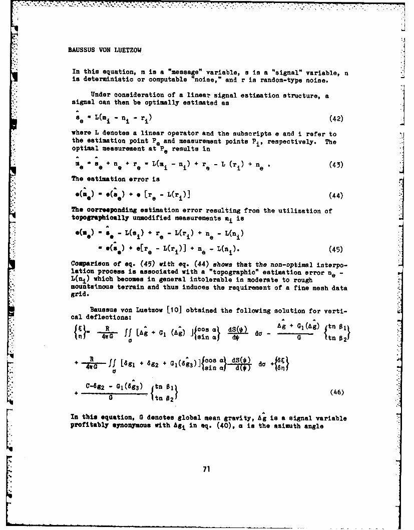
BAUSSUS VON LUETZOW
In this equation, m is a "message" variable, a is a "signal" variable, nis deterministic or computable "noise," and r is random-type noise.
Under consideration of a linear signal estimation structure, asignal can then be optimally estimated asAIe = L(mi ni ri) (42)
where L denotes a linear operator and the subscripts e and i refer tothe estimation point Pe and measurement points Pi, respectively. Theoptimal measurement at P5 results in
me M se + ne + re a L(mi " ni) + r - L (ri) + ne . (43)
The estimation error is
.() •(s + e [r. - L(ri (44)
The oorresponding estimation error resulting from the utilization oftopographically unmodified measurements mi is
*(me) so e L(si) + r - L(ri) + ne - L(ni)
' e (; e) + e[r e - L(ri)] + ne - (ni)" (45)
Comparison of eq. (45) with eq. (44) shows that the non-optimal interpo-- .lation process is associated with a "topographic" estimation error ne -
niL(n) which becomes in general intolerable in moderate to roughmountainous terrain and thus induces the requirement of a fine mesh datagrid.
Baussus von Luetzow [10] obtained the following solution for verti-
cal deflections: A
R " + , cos a dS-) Ag + (Ag) tn 01i8"1 i f A G I (Ag) |sin a G dtn - 2
am4wG ff La,+62+1163 sin al d d a n .
C-9 2 G1(89 3 ) {tn } (46).i. + " G " ' ' tn 02 .-
In this equation, 0 denotes global mean gravity, Ag is a signal variableprofitably synonymous with Agi in eq. (40), a is the auimuth angle
71
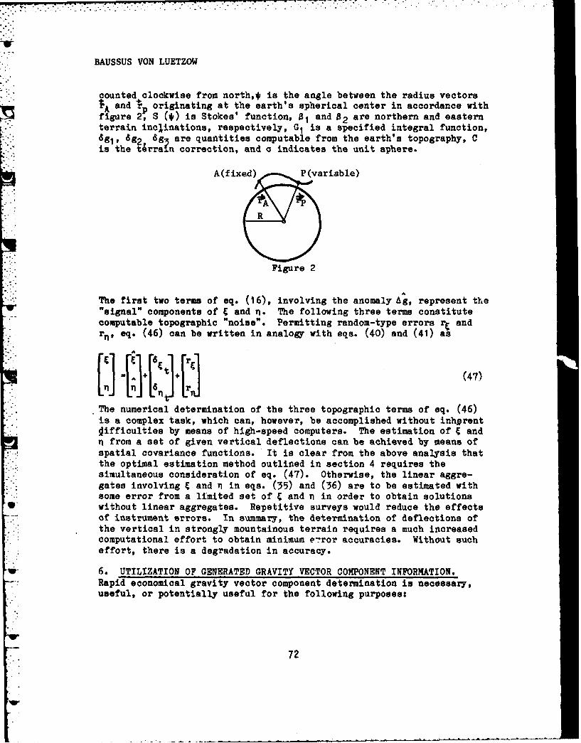
BAUSSUS VON LUETZOW
counted clockwise from north,* is the angle between the radius vectors
tA nd + originating at the earth's spherical center in accordance withfigure 2, S (#) is Stokes' function, 01 and 02 are northern and easternterrain inclinations, respectively, G1 is a specified integral function,6g1 , 6g2 6g are quantities computable from the earth's topography, Cis the terrafn correction, and o indicates the unit sphere.
A(fixed) P(variable)
R
Figure 2
The first two terms of eq. (16), involving the anomaly Ag, represent the"signal" components of C and n. The following three terms constitutecomputable topographic "noise". Permitting random-type errors rt andr., eq. (46) can be written in analogy with eqs. (40) and (41) as
+ C,/+/r,1(47)~ 6 r1n] I 6n J+[rj
The numerical determination of the three topographic terms of eq. (46)is a complex task, which can, however, be accomplished without inhorentOifficulties by means of high-speed computers. The estimation of E andn from a set of given vertical deflections can be achieved by means ofspatial covariance functions. It is clear from the above analysis thatthe optimal estimation method outlined in section 4 requires thesimultaneous consideration of eq. (47). Otherwise, the linear aggre-gates involving 9 and n in eqs. (35) and (36) are to be estimated withsome error from a limited set of E and n in order to obtain solutionswithout linear aggregates. Repetitive surveys would reduce the effectsof instrument errors. In summary, the determination of deflections ofthe vertical in strongly mountainous terrain requires a much increasedcomputational effort to obtain minimum e~ror accuracies. Without sucheffort, there is a degradation in accuracy.
6. UTILIZATION OF GENERATED GRAVITY VECTOR COMPONENT INFORMATION.Rapid economical gravity vector component determination is necessary,useful, or potentially useful for the following purposes:
72
BAUSSUS VON LUETZOW
(a) Transformation of astronomic coordinates and astronomic azi-muths into ideal terrestrial-geodetic coordinates and geodetic azimuths,requiring knowledge of absolute deflections of the vertical, indispens-ible for long range ballistic missiles.
* (b) Establishment of a three-dimensional anomalous gravity poten-tial T or analytical upward continuation of first order derivatives ofAg, n, and E from discrete measurements thereof at the earth's surface,to extend over relatively large areas, indispensible for long rangeballistic missiles with inertial guidance.
(c) Adjustment of geodetic networks.
(d) Geophysical prospecting including estimation of the deriva-rive- - 2GR--1N + GR- tn* -G (3C + _
) in semi-flat terrain
ar 5- Ywhere N stands for geoidal undulation or height anomaly.4
(e) Determination of geoidal differences on land.
(f) Construction of regional gravity anomaly and vertical deflec-tion networks with mesh sizes Ax - Ay of about 5 Km as input information
for highly accurate gravity programmed inertial surveying systems.
(g) Accuracy improvement of medium range ballistic missiles inconjunction with meteorological corrections and of cruise missiles byutilization of vertical deflection data in accessible areas.
7. CONCLUSIONS. The determination of vertical gravity vector compo-nents or gravity anomalies by means of inertial and boundary data hasbeen very promising as to rapidity and accuracy. High accuracy estima-tion of horizontal gravity vector components or deflections of thevertical from inertial and boundary data requires the installation of
*. gryoscopes, accelerometers, and velocity quantizers with small errorvariances and short correlation times, the development of sophisticatedestimation methods consistent with an outlined structure, and, probably,a three-dimensional Kalman filter. Deflection accuracy in stronglymountainous terrain is degraded. For this reason, a maximum rms errorrequirement of about 0.3 arcsec in both semi-flat and mountainous ter-rain may only be achieved by a gradiometer-aided inertial system. Such
4. See Telford et al [11], pp. 7-104, for geophysical applications andHeiskanen and Moritz [12], p. 117, for the equation.
73
7.
BAUSSUS VON LUETZOW
a system would also be beneficial for the location of smaller subterra-neous mass anomalies. An effective estimation of gravity anomalies anddeflections of the vertical in mountainous terrain from data at pointsseparated by distances of the order 5-10 Km is possible with consid-erable computational effort under utilization of the developed equationsand employment of spatial covariance functions. Numerous military andnon-military applications of gravity vector component information gener-ated by inertial and auxiliary data do exist. Gradiometer-aided iner-tial systems offer additional advantages.
REFERENCES
[1]. Litton Systems, Inc. Geodetic Platform Development Program,Public. No. 12987, Woodland Hills, CA 91364, 1974.
[2]. Huddle, J. The Measurement of the Chanj- in the Deflection of theVertical betwen Astronomic Stations with a Schuler-Tuned InertialSystem. Litton Guidance & Control Systems, Woodland Hills, CA 91364,1977.
[3]. Litton Systems, Inc. P-1OO Inertial Instrument, A-1000 Acceler-ometer. Public. No. 12391 A. Woodland Hills, CA 91364, 1973.
[4]. Litton Systems, Inc. Addendum to Feasibility Test Program forMeasurement of Gravity Anomaly Changes Using 2 Micro-G Accelerometer inInertial Platform. Document No. 402414. Woodland Hills, CA 91364,1975.
[5]. Litton Systems, Inc. Proposal for Position and AzimuthDetermining System (PADS), Vol. II - Technical Proposal. WoodlandHills, CA 91364, Sept. 1970.
[6]. Moritz, H. Current Determination of Vertical Deflections. Proc.1st Internatl. Symp. on Inertial Technology for Surveying and Geodesy,Ottawa, Canada, Oct. 1977.
[7]. Schwarz, K. P. Inertial Surveying Systems - Experience andPrognosis. Paper, presented at the FIG-Symposium on Modern Technologyfor Cadastre and Land Information Systems, Ottawa, Canada, Oct. 1979.
[8]. Huddle, J. The Measurement of the Change in the Deflection of theVertical with a Schuler-Tuned North-Slaved Inertial System. LittonGuidance & Control Systems, Woodland Hills, CA. 91364, 1977.
[9]. Baussus von Luetzow, H. A New Method for the Determination ofL Deflections of the Vertical from Astrogeodetic and Inertially Derived
74

BAUSSUS VON LUETZOW
Data. Paper, presented at the Spring Meeting of the Am. Geoph. Union,Baltimore, MD., May 1981.
10]. Baussus von Luetzow, H. On the Interpolation of GravityAnomalies and Deflections of the Vertical in Mountainous Terrain. Proc.VIth Internatl. Symp. on Geodetic Computations, Munich, W. Germany, Aug.- Sept. 1981.
[iI]. Telford, W., L. Geldert, R. Sheriff, and D. Keys, AppliedGeophysics, Cambridge Univ. Press, Cambridge CB2 IRP, England, 1976.
[12]. Heiskanen, W. and H. Moritz. Physical Geodesy, W. H. Freeman andCo., San Francisco and London, 1967.
75q.
BERTIN & GOODYEAR
MULTIPLE LAUNCH ROCKET SYSTEM (MLRS) FUZE (U)JOHN J. BERTIN, DR.
THE UNIVERSITY OF TEXAS AT AUSTINAUSTIN, TEXAS 78712
*RICHARD L. GOODYEAR, MAJU.S. MILITARY ACADEMY
WEST POINT, NEW YORK 10996
1. INTRODUCTION
When the U.S. Army began limited production of the fuze for therocket warhead of the Multiple Launch Rocket System (MLRS), it wasnecessary to develop improved methods of testing fuzes as they came offthe assembly line. Since the fuze contained a fluidic power supplythat had never been type-classified, methods associated with previousbattery-powered fuzes were inadequate for the production specification.Also during the validation and maturation phases of the developmentprogram, considerable testing in the laboratory, in wind tunnels, andin flight tests showed that laboratory tests in early specificationsdid not indicate adequately how a fuze would perform in actual flight.A key deficiency was the inability to duplicate in the laboratory theconditions near the summit of the rocket's trajectory. Operating thefluidic generator from an air source up to 14 kilopascals aboveatmospheric pressure approximated the expected pressure differencebetween the entrance and exit of the generator, but it failed to dup-licate the effects of the air's speed.
The power supply project team at the U.S. Army Harry DiamondLaboratories (HDL) proposed a solution in the form of a relativelyinexpensive high altitude chamber, which would duplicate both of theseflight variables, and which could be incorporated into the fuzecontractor's test equipment. Implementation of this proposal requireda better understanding of the conditions of the air flow around thefuze ogive and through the generator. Consequently, HDL conducted atest program in the Aerodynamic Wind Tunnel at the Arnold EngineeringDevelopment Center. Test conditions included free-stream Mach numbersfrom 0.95 to 1.3 over a range of free-stream densities that simulatedaltitudes from 15.2 Km to 21 Km. The fuze ogive was instrumented withboth static and pitot pressure probes, from which the pressure data wereanalyzed to describe the internal and external flow fields.
77
A1
FtD-Ai28 811 PROCEEDINGS OF THE 1982 ARMY SCIENCE CONFERENCE HELD RT 2/6THE UNITED STATES..(U) DEPUTY CHIEF OF STAFF FORRESEARCH DEVELOPMENT AND ACQUISITIO. iS JUN 82
UNCLASSIFIED F/G 5/2 , N
EIEEEIEEEEEEONIEhhI-mohhhIsmhhhhohhhhhh
-. ~I L28-~
L IIOIL io
~~~~~~~~~~~MICROCOPY RSLTOTETCATINIOL RENJMT TESTCOW~133
MCIp MICOCOY NOUJI TEST CHART NT&MMO ADM--NATIONA UREM OF STANDARDS-1963-A
-m-1
MICROCOPY RESOfLUTMN TEST CHART- NATIONAL UUEDIJ OF STANOARDS-1963-A- - -
us.0 I 7L
MIcROCOP RESOLTIN TEST CHR MICOP RESMOLU IMs CWWF%MftIONLMMAEA Of ZTANDDUS 19SANAIALUfA MbiSS5
N -- o l jm
BERTIN & GOODYEAR
2. EXPERIMENTAL PROGRAM
The general features of the nose cone are illustrated in the sketchpresented in Figure 1. A sectioned drawing has been used to present the
2. details of the external geometry and of the generator installation. Theair that drives the fluidic generator enters the "inlet hole" in thestagnation region of the blunt face, passes through the generator assemblyand into the (internal) chamber. it then flows through the exhaust portsinto the (external) cavity. This use of the words "chamber" for theinternal region and "cavity" for the depression in the external surfacewill be retained throughout this report. The 24 exhaust ports, which are0.269 cm in diameter, are equally distributed circumferentially and arelocated in a shallow cavity that begins 3.259 cm (x - 0.423 xo) aft of thetip of the fuze. As shown in figure 1, x is the longitudinal position,as measured from the model nose. The reference length, xo-, was chosen tobe 7.696 cm, the coordinate of the most-downstream pressure tap.
The nose cone used in the initial phase of the test program wasinstrumented with 29 surface pressure taps (or orifices), of which 21
Reglan ~(External) (ienl
*: x
-- - .12.370
0.348- --
3g
- SAM__.h
Figure 1. - Sketch of the Army/MLRS Fluidic-Generator Fuze-Assembly.
78
78
I5
-j.'I'':''./. ,°; "." "" ' . '"'', -.- ,," " ","L' ,''." ' ' ' ' ". .'. . . """"""% . . .......
BERTIN & GOODYEAR
were on the external surface and 8 were on the internal surface. Thelocations of the orifices for which data are presented in this paper areillustrated in Figure 2.
3. RESULTS
Static pressures and Pitot pressures were measured both on theexternal surface and on the internal surface of a full-scale fluidicgenerator/fuze assembly of the MLRS in the Aerodynamic Wind Tunnel (4T)at AEDC. The pressure data from these tests are discussed in this section.
3.1 External Pressures for 0* Angle of Attack
3.1.1 Pressures on Flat Face (x - 0.0)
A strong, detached shock wave forms in front of a blunt bodywhen it is placed in a supersonic stream. The shape of the bow shock wave': Expansion fart
Shock at and Recomrnp, sion/T. 22; opmfon for cavit
T. .
To 1
Fgr 2 lSle .i. i i l a fi- ~ eaves chamber
Resr o f poh exhaust ports
, ,for the Resoa tor- .# ercto.:: nozzle- Region
centerline
SInlet 251 centerlin"-,Ihole I- Tr .16 (located in the external surfte
btwen the exhaust ports)
through exhaust .... ...
_ Figure 2. -Sketch illustrating instrumentation locations and features,
! of proposed flow model.,
79
- _____. ./ .. .. ,.... ,....... .................... ,.................... • ..... ,.... .... . . -.
BERTIN & GOODYEAR
'for supersonic flow past the nose
cone is shown in the schlieren photo-graph frou a previous test program(1) that is presented in Figure 3.Since the Mach number of the flowrepresented by the schlieren photo-graph is greater than those of thepresent program, the stand-off dis-tance of the bow shock wave is muchless than would be the case for thepresent flows. This is to be ex-pected. Nevertheless, the photographprovides valuable insights into theflow. Because the bow shock wave iscurved, the static pressure on thesurface should decrease from a valueof the stagnation pressure downstreamof a normal shock wave, Pt2 , at theaxis of symmetry to the sonic valueat the corner. This pressure varia- Figure 3. Schlieren photograph fromtion is illustrated by the pressure the tests of ref. 1,distribution that was presented else- M" - 1.5.
: where (2) for a free-stream Mach
i r-Top 351
Pitot probes (32or 132)
Data -from ref.2 for aflat-faced nose. (M *2.01)
1.0 05 0
Dkmwdios in cm
Figure 4. - Nose-region instrumentation and pressure distributions for a
flat-faced cylinder (ref. 2).
80
-,4.' 2.,:... .. ,, ;., ;+ ,,..,. +.+ . . . , .,., . . . . . . ." . . '. . ." + ,. .- ,,.,. .
l'p pp;<+.', .+.., , +++, .., ,t:+ .+.. +: , . .. .. ... .. . 4.. . . . . . .
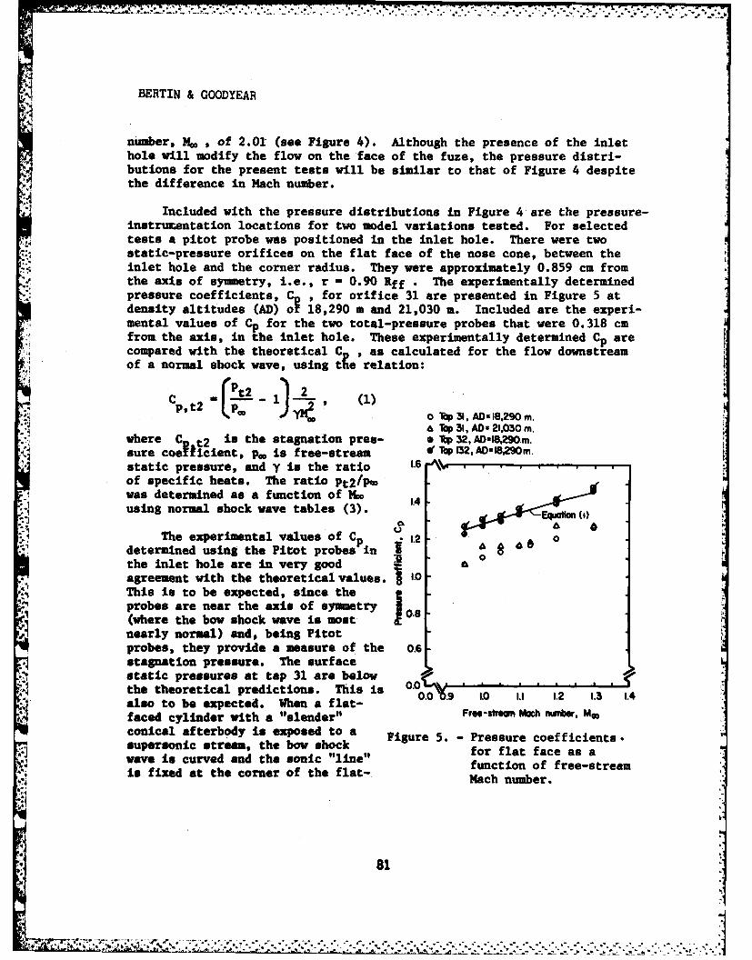
BERTIN & GOODYEAR
number, L. , of 2.01 (see Figure 4). Although the presence of the inlethole will modify the flow on the face of the fuze, the pressure distri-butions for the present tests will be similar to that of Figure 4 despitethe difference in Mach number.
Included with the pressure distributions in Figure 4 are the pressure-instrumentation locations for two model variations tested. For selectedtests a pitot probe was positioned in the inlet hole. There were twostatic-pressure orifices on the flat face of the nose cone, between theinlet hole and the corner radius. They were approximately 0.859 cm fromthe axis of symmetry, i.e., r - 0.90 Rff . The experimentally determinedpressure coefficients, C, , for orifice 31 are presented in Figure 5 atdensity altitudes (AD) o 18,290 m and 21,030 m. Included are the experi-mental values of Cp for the two total-pressure probes that were 0.318 cmfrom the axis, in the inlet hole. These experimentally determined C p arecompared with the theoretical C , as calculated for the flow downstreamof a normal shock wave, using the relation:
2!t2
cc o To )31,AD a 8,290rn, ,& Top 31, AD z 21,030 m.where C t2 is the stagnation pres- * Top 32, AD-lC90m.
sure coeficient, p. is free-stream f Tap 132, AD-1829Om.static pressure, and y is the ratio 1.6...........of specific heats. The ratio Pt2/Pwwas determined as a function of MH0 1.4using normal shock wave tables (3). 1.4
The experimental values of Ci 1.2 0
determined using the Pitt probesin a
the inlet hole are in very good
agreement with the theoretical values. 1.0This is to be expected, since the gprobes are near the axis of symmetry !(where the bow shock wave is most 0.8
Anearly normal) and, being Pitotprobes, they provide a measure of the 0.6stagnation pressure. The surfacestatic pressures at tap 31 are belowthe theoretical predictions. This is 0.0' .. . . . . .4
also to be expected. When a flat-faced cylinder with a "slender" Frt-swms Mth nmber, Maconical afterbody is exposed to a Figure 5. Pressure coefficients.supersonic stream, the bow shock F. for flat face as awave is curved and the sonic "line" function of free-streamis fixed at the corner of the flat-. Mach number.
44-0
81?
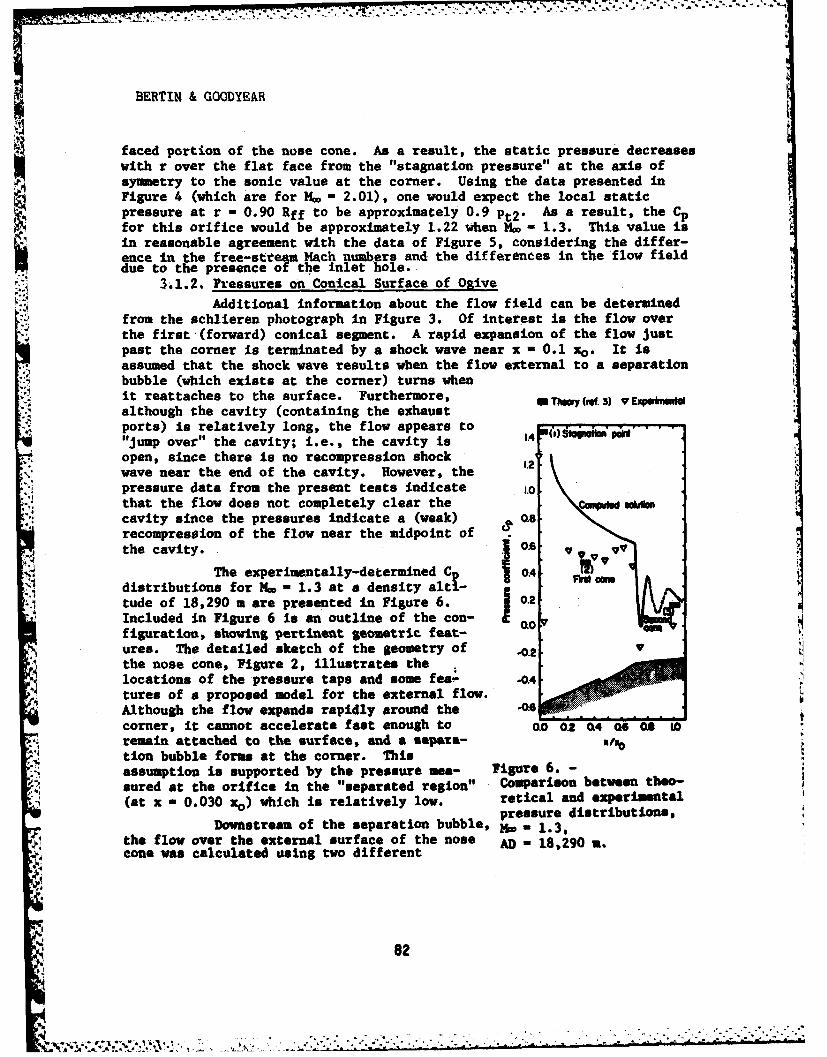
BERTIN & GOODYEAR
faced portion of the nose cone. As a result, the static pressure decreaseswith r over the flat face from the "stagnation pressure" at the axis ofsymmetry to the sonic value at the corner. Using the data presented inFigure 4 (which are for M. - 2.01), one would expect the local staticpressure at r - 0.90 Rff to be approximately 0.9 Pt2" As a result, the Cfor this orifice would be approximately 1.22 when M - 1.3. This value isin reasonable agreement with the data of Figure 5, considering the differ-ence in the free-stte~a Mach numbers and the differences in the flow fielddue to the presence of the inlet hole.
3A~.2. Pressures on Conical Surface of OgiveAdditional information about the flow field can be determined
from the achlieren photograph in Figure 3. Of interest is the flow overthe first (forward) conical segment. A rapid expansion of the flow justpast the corner is terminated by a shock wave near x - 0.1 xo . It isassumed that the shock wave results when the flow external to a separationbubble (which exists at the corner) turns whenit reattaches to the surface. Furthermore, *Thsy(,r 3) '
although the cavity (containing the exhaustports) is relatively long, the flow appears to () im, ."Jump over" the cavity; i.e., the cavity is 14
open, since there is no recompression shock 2wave near the end of the cavity. However, thepressure data from the present tests indicate 1.0
that the flow does not completely clear thecavity since the pressures indicate a (weak) asrecompression ofthe flow near the midpoint of
the cavity. 0.6 V V
The experimentally-determined C 0.4 Mdistributions for 16 - 1.3 at a density alti- _tude of 18,290 m are presented in Figure 6. J 0.2
Included in Figure 6 is an outline of the con- o.0figuration, showing pertinent geometric feat-ures. The detailed sketch of the geometry ofthe nose cone, Figure 2, illustrates thelocations of the pressure taps and some fea- -4,
tures of a proposed model for the external flow.Although the flow expands rapidly around the 4 .
corner, it cannot accelerate fast enough to 0. 02 040 0 1remain attached to the surface, and a separa-tion bubble forms at the corner. Thisassumption is supported by the pressure mea- Figure 6. -
sured at the orifice in the "separated region" Comparison between theo-(at x - 0.030 xo ) which is relatively low. retical and experimental
pressure distributions,Downstream of the separation bubble, M. - 1.3,
the flow over the external surface of the nose AD - 18,290 a.cone was calculated using two different
82
~. . . . . . . .. . . . . .. . . . . . . . . .... ....-. ... •• ' . - " . "- . '. . . .. -. .-.. .. --. . --.
BERTIN & GOODYEAR
approaches. Theoretical values of C were calculated using standard
normal shock-wave tables and graphs for sharp cones. Values are presented
(1) for the stagnation point (Cp - 1.45),(2) for the forward conical segment (C - 0.48, the value for a sharp(os0u
cone whose half-angle is 20.5*), and(3) for the second conical segment (Cp - 0.16, the value for a sharp "
cone whose half-angle is 10.75°).
Also included is the theoretical distribution computed using the Univer-
* sity of Texas' Missile Aerodynamics Code, which is similar to that de-scribed by Moore and Swanson (4). In preparing the geometric input for
the computer solution, the presence of the cavity in the external contour
was omitted and the nose cone was represented by two conical frustums.
Because of the extreme bluntness of the nose cone, the computed solutionshould be considered approximate.
Both the computed solution and the "sharp-cone" approximations (3)provide a reasonable estimate of the pressures on the downstream (second)
conical segment, i.e., for x > 0.716 xo . The computer solution even
predicts the rapid "overexpansion" that takes place downstream of the
intersection of the two conical segments. An oscillatory character which
appeared in the computed solution for the pressure distribution for the
second conical segment is represented in Figure 6 by a broken line. Thebroken-line representation was used since the variation may be a com-
putational peculiarity and not a flow phenomenon.
The most significant differences between the theoretical values and
the experimental values occur on the forward conical surface and in the
cavity in this region. Note that the upstream edge of the cavity is at
x - 0.423 x0. The experimental pressures at the first tap of the cavity(tap 17 at x - 0.482 xo) are essentially equal to those upstream of the
cavity. The fact that the pressure did not decrease when the flow sepa-
rated at the cavity is attributed to the relatively shallow depth of the
cavity. The pressure increase at the three pressure taps in the down-
stream region of the cavity (0.551 xo I x < 0.689 xo), reflects the
recompression of the flow as it reattaches to the surface. Thus, if one
assumes that a tangent-cone approximation is valid for the forward conical
surface and that a recompression pressure rise occurs at the downstream
end of the cavity, one can explain the fact that the pressures measured
at the taps between 0.551 xo and 0.689 x. are above the Ames theoreticalestimates (3). Since both theoretical models are approximate, close
correlation with the data should not be expected. Each assumed modelprobably contains elements of the actual flow field.
The effect of HMo on the pressure distribution is illustrated by the
data presented in Figure 7. This pressure distribution is for a density
altitude of 21,030 a. There is a consistent trend with Mach number at all
the orifices from x = 0.030 xo to x - 1.000 xo . That is, the ratio P/Pt2
II I
83
AL-
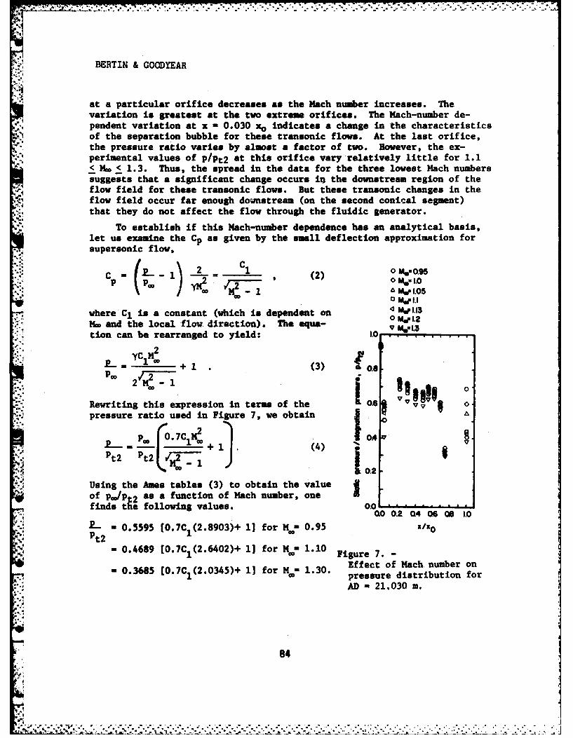
BERTIN & GOODYEAR
*! at a particular orifice decreases as the Mach number increases. Thevariation is greatest at the two extreme orifices. The Mach-number de-pendent variation at x - 0.030 xo indicates a change in the characteristicsof the separation bubble for these transonic flows. At the last orifice,the pressure ratio varies by almost a factor of two. However, the ex-perimental values of P/Pt2 at this orifice vary relatively little for 1.1< Mw < 1.3. Thus, the spread in the data for the three lowest Hach numberssuggests that a significant change occurs in the downstream region of theflow field for these transonic flows. But these transonic changes in theflow field occur far enough downstream (on the second conical segment)that they do not affect the flow through the fluidic generator.
To establish if this Mach-number dependence has an analytical basis,let us examine the Cp as given by the small deflection approximation for
* supersonic flow,
C ( 2 =M , (2) 0 me. .0Go1 Me L05
a MIjI.I
where C1 is a constant (which is dependent on OmI.Mw and the local flow. direction). The equa- Ms-L3tion can be rearranged to yield: . .
C 2
S+ 1 (3) 0.i;2 v2 - 1
0
Rewriting this expression in terms of the 0.6 0pressure ratio used in Figure 7, we obtain £
p., 0.7C M2 104P 1 +11 (4) *
pt2 Pt2I "jFM j *.)0.2
Using the Ames tables (3) to obtain the valueof P-/P 2 as a function of Mach number, one Ifinds te following values. 0.0. ..........
400 0.2 04 06 08 1.O
* 0.5595 [0.7C1 (2.8903)+ 1] for M. = 0.95 X/X0Pt2
. 0.4689 [0.7C (2.6402)+ 1] for H - 1.10Fiue7
- 0.3685 [0.7C1 (2.0345)+ 11 for M,4= 1.30. Effect of Mach number on,. pressure distribution for
AD 21,030 m.
.8
84
r4
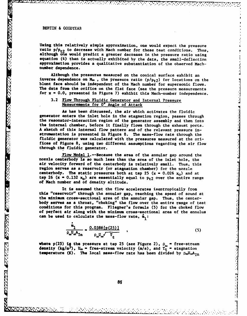
.BERTIN & GOODYEAR
Using this relatively simple approximation, one would expect the pressureratio P/Pt2 to decrease with Mach number for these test conditions. Thus,
.4 although one would predict a greater decrease in the pressure ratio usingequation (4) than is actually exhibited by the data, the small-deflection
approximation provides a qualitative substantiation of the observed Mach-number dependence.
Although the pressures measured on the conical surface exhibit aninverse dependence on Mw , the pressure ratio (P/Pt2) for locations on theblunt face should be independent of the Mach number for supersonic flows.The data from the orifice on the flat face (see the pressure measurementsfor x - 0.0, presented in Figure 7) exhibit this Mach-number independence.
3.2 Flow Through Fluidic Generator and Internal PressureMeasurements for 0 Anale of Attack
As has been discussed, the air which activates the fluidicgenerator enters the inlet hole in the stagnation region, passes throughthe resonator-interaction region of the generator assembly and then intothe internal chamber, before it finally flows through the exhaust ports.A sketch of this internal flow pattern and of the relevant pressure in-strumentation is presented in Figure 8. The mass-flow rate through thefluidic generator was calculated with the pressures measured at the ori-fices of Figure 8, using two different assumptions regarding the air flowthrough the fluidic generator.
Flow Model 1.--Because the area of the annular gap around thenozzle centerbody is so much less than the area of the inlet hole, theair velocity forward of the centerbody is relatively small. Thus, thisregion serves as a reservoir (or stagnation chamber) for the nozzlecenterbody. The static pressures both at tap 25 (x - 0.026 xo) and attap 26 (x - 0.132 xo) are essentially equal to Pt2 over the entire rangeof Mach number and of density altitude.
It is assumed that the flow accelerates isentropically fromthis "reservoir" through the annular gap, reaching the speed of sound atthe minimum cross-sectional area of the annular gap. Thus, the center-body serves as a throat, "choking" the flow over the entire range of testconditions for this program. Fliegner's formula (5) for the choked flowof perfect air along with the minimum cross-sectional area of the annuluscan be used to calculate the mass-flow rate, il
PUA 0.0386[P(25)) 5i' - A (5) .cocWoIn 0U T
where p(25) i the pressure at tap 25 (see Figure 2), poo - free-streamdensity (kg/m), U 0 - free-stream velocity (m/s), and Tt - stagnationtemperature (K). The local mass-flow rate has been divided by pmUAoin
85
...... ( The lc mas.... ... s I.--L IM. .. - ***- .-
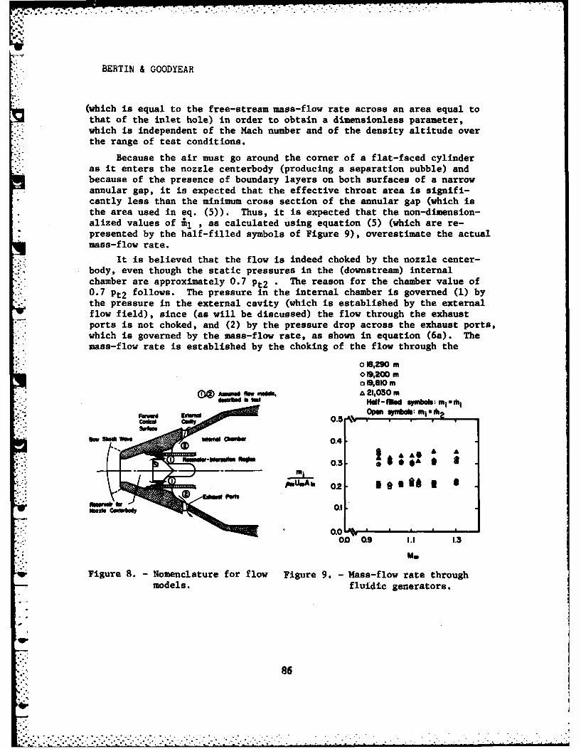
BERTIN & GOODYEAR
(which is equal to the free-stream mass-flow rate across an area equal tothat of the inlet hole) in order to obtain a dimensionless parameter,which is independent of the Mach number and of the density altitude overthe range of test conditions.
Because the air must go around the corner of a flat-faced cylinderas it enters the nozzle centerbody (producing a separation bubble) andbecause of the presence of boundary layers on both surfaces of a narrowannular gap, it is expected that the effective throat area is signifi-cantly less than the minimum cross section of the annular gap (which isthe area used in eq. (5)). Thus, it is expected that the non-dimension-alized values of 1 , as calculated using equation (5) (which are re-
e. presented by the half-filled symbols of Figure 9), overestimate the actualmass-flow rate.
- .. It is believed that the flow is indeed choked by the nozzle center-body, even though the static pressures in the (downstream) internalchamber are approximately 0.7 Pt2 . The reason for the chamber value of0.7 Pt2 follows. The pressure in the internal chamber is governed (1) bythe pressure in the external cavity (which is established by the externalflow field), since (as will be discussed) the flow through the exhaustports is not choked, and (2) by the pressure drop across the exhaust ports,which is governed by the mass-flow rate, as shown in equation (6a). Themass-flow rate is established by the choking of the flow through the
0 1,29 m* c9,200 m
a I9.810AWMW () a 21,030 m
Half-fllW symbols: miuh IS Open ey ibo: mi 1 2
0.5 AN .
-Ma"A A A0.3 * *
.UA 02 * m
0.000 0.9 1.1 1.3
Me
Figure 8. - Nomenclature for flow Figure 9. - Mass-flow rate through
models. fluidic generators.
86
DERTIN & GOODYEAR
- sle ce bt bOdy. The static pressure Incre from the sonic value(0 .53 pa) at tbh throat of the nozle centarbody to 0.7 Pt2 P the value
-Ir.. the Isternal chamber, as it flows through the resonator-Interactionregion of the generator assembly (see Figures 1 aid 8) and into the in-termal chamber.
Tb. conclusion that the flow is choked not at the exhaust ports butat the nozle eetsbody over the range of test conditions is veryImportant. It has been shown that the pressure ratio (p/pt2) for thes*parted regio Of the external cavity is a well-behaved function of thefEee-stresa Mah number and is independent of density altitude. Sincethe pressure drop across the eA4st ports is relatively smal and is afunction of the too-flow rate through the fluidic generator, the pressurein the Internal aumber (whith is the, "back pressuret"for the resonator-Interaction ragiew of the- fluidic gener~ator) follv the extetnal pressure.Novever, since the 'flow is choked by the nozia ceterb~dy, the inletpreesue for the resaator-Iieetgction region is i'fixed ftia4tion, ofP O; 5), the onicJ vaue). It i. expected that the details of theflow ftold" in -the* resontator depend on the pr'essure difference$ across it.
~ or the gecond f 19lodal the Volumetric f 1ev-rate,v-s calult vefte the equation; for- ubsonic flow through a sharp-
Q * .1 ~ ~ ,(6a)
where for the orfoiceratias and for tie Reyfolds numbers of the present, ~ ~~tests,. . " ".
Aurh am *tpk 1 asme tte, a eaation a f. the f lew from theIstemi Chamber tbroogtba heemwt. p""t $s such that.
p+ (c
The mss-flto rates tulcuate dm ar presented as a function of
]valuesof th pressure raio tp(1)IItp(27).] indicate tht the flow intisregio n ~O LncopreMsible. Thus, the asuptions rade in developinflow mdel 2r a qite taisti. Since the two pressures needed to
-'7
m~ ~ ~N ' a' 1,8mra9,, (sothe opme, gymbals) N+ +-+ : . ,*+* e....riu,'.,'tel.,.y. d..-.,..-...-_:,
BERTIN & GOODYEAR
calculate the flow field were measured directly it iq believed that the3 mass-flow rates calculated using equation (7), I.e., m2 , are the morerealistic of the two flow models.
4. CONCLUSIONS
This analysis showed that pressures measured at the inlet hole to thefluidic generator are in close agreement with those given by normal shockrelations. Over the external surface of the ogive, the ratio of localstatic pressure to stagnation pressure measured at the nose, P/Pt2 de-creased as the free stream Mach numbers increased. Within this trendexisted regions of expansion and compression which were a result of theogive's geometry and the injection of the air exhausted from the fluidicgenerator. Theoretical models predicted reasonably well the dependenceon Mach numbers of P/Pt2 as well as the relative values of P/Pt2 atdifferent points on the ogive. Pressures measured at the entrance andexit of the region occupied by the generator permitted calculation of themass flow rate through the fuze. This analysis verified that the keyfactors that should be duplicated in laboratory tests were the pressuresat the generator's entrance and at the exhaust ports in the ogive; butthe most significant result was the accumulation of a data base of theactual pressures to be associated with desired combinations of Machnumber and altitude. Consequently, the high altitude chamber proposedto test MLRS fuzes has been incorporated into the product specificationand used with confidence in the quality assurance program of the con-tractor.
LITERATURE CITED
1. R. L. Goodyear and H. Lee, Performance of the Fluidic Power Supplyfor the XM-445 Fuze in Supersonic Wind Tunnels, HDL-TM-81-4,Feb. 1981, Harry Diamond Laboratories.
2. J. C. Boison and H. A. Curtiss, An Experimental Investigation ofBlunt Body Stagnation Point Velocity Gradient, ARE Journal, Feb.1959, Vol. 29, No. 2, pp. 130-135.
3. Ames Research Staff, Equations, Tables, and Charts for CompressibleFlow, Report 1135, 1953, NACA.
4. F. G. Moore and R. C. Swanson, Jr., Aerodynamics of Tactical Weaponsto Mach Number 3 and Angle of Attack 150, Part I--Theory andApplication, NSWC/DL TR-3584, Feb. 1977, Naval Surface Weapons Center.
5. A. H. Shapiro, The Dynamics and Thermodynamics of Compressible Fluid* Flow, Ronald Press, New York, 1953.
6. Staff, Flow of Fluid Through Valves, Fittings, and Pipes, TechnicalPaper No. 410, The Crane Company.
88
a~~~~t .j .1_..---
-7 '
Bhatt
THERMAL FATIGUE BEHAVIOR OF FP ALUMINA/MAGNESIUM COMPOSITES
*Ramakrishna T. Bhatt, PhD
Propulsion Laboratory, USARTL(AVRADCOM)Cleveland, Ohio
Intrbduction
Composites of magnesium alloys reinforced with FP-Alumina are beingconsidered for aerospace applications because of their high specificstrength and modulus, and because of their relative ease of fabrication.Some of these applications require repeated high temperature exposure ofthe composite material for extended periods of time. In a recent study,Bhatt, et al. () have evaluated the effects of isothermal and cyclicexposure on the room temperature mechanical properties of unidirectionallyreinforced FP-A1203 /EZ33 magnesium composites. Results of this studyindicate no significant loss in the room temperature axial tensile strengthand dynamic flexural modulus of composites thermally cycled between 500 and250 0 C or of composites isothermally heated at 350 0 C for up to 150 hours from
4the strength and modulus data for the as-fabricated composites. In con-trast, thermal cycling between 50Oand 3000 C caused considerable loss inboth room temperature strength and modulus. The major causes of strengthdegradation were attributed to softening and cracking of the matrix anddebonding of the fibers from the matrix.
The objective of this investigation was to study the effects of matrixcomposition on thermal fatigue behavior of FP-A1 2 0 3 /magnesium composites asdetermined by tensile stength and modulus measurements after cyclicexposure.
In this study, 55 volume percent fiber unidirectionally aligned compos-ites were exposed in air to temperatures of either 2500 or 3500C for up to3000 cycles. Isothermal exposure at 350 0C was used as a baseline toevaluate the additional effect of cycling. Metallographic and fractographicstudies were made on untreated and thermally cycled composite material in anattempt toward understanding the failure mechanisms involved.
89
4
,. t ,r ,, ,,, " ,,, ,.., ,,."., ,,,. .,a ., l,.. ,lt. -: • " " " " - ' ." '_- " . " '_,. -.- ,',,
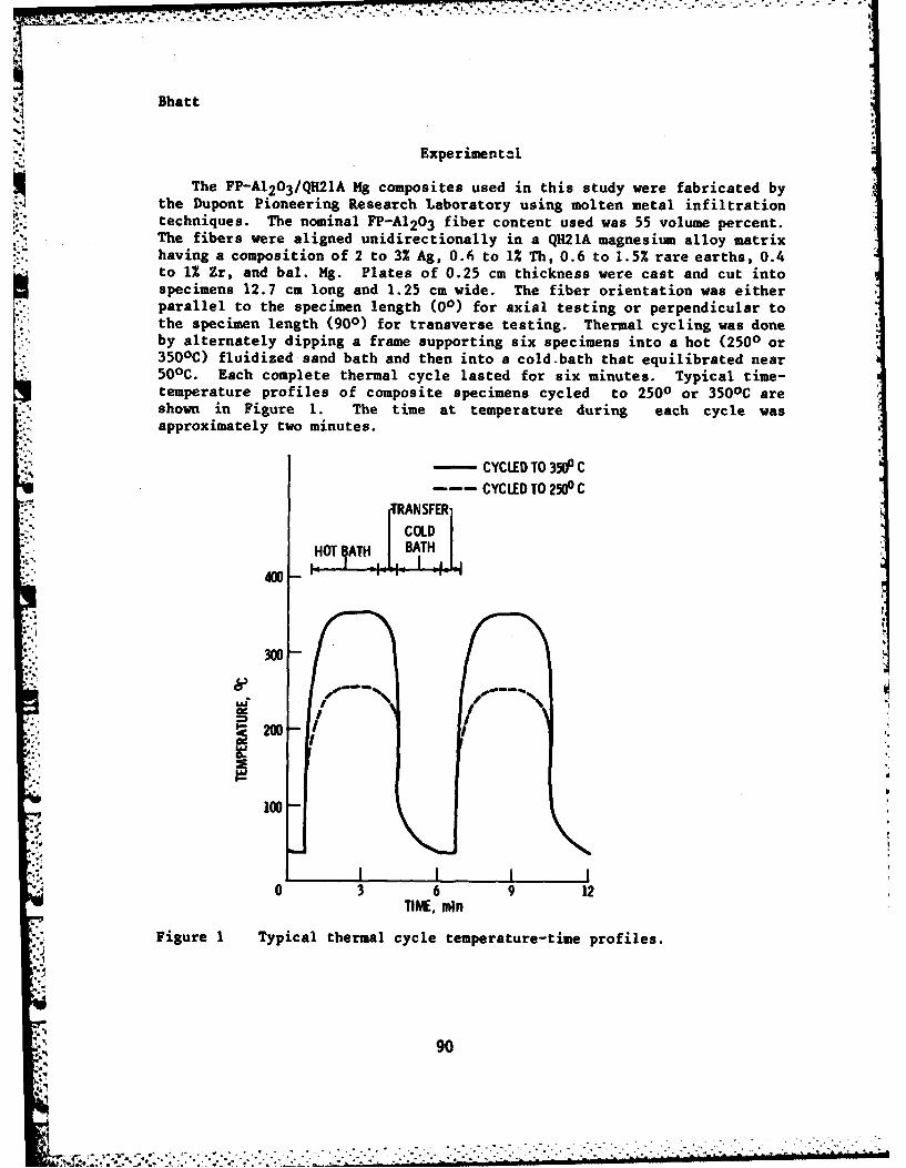
7!Bhatt
Experimental
The FP-Al203/QH21A Mg composites used in this study were fabricated bythe Dupont Pioneering Research Laboratory using molten metal infiltrationtechniques. The nominal FP-A1203 fiber content used was 55 volume percent.The fibers were aligned unidirectionally in a QH21A magnesium alloy matrixhaving a composition of 2 to 3% Ag, 0.6 to 1% Th, 0.6 to 1.5% rare earths, 0.4to 1% Zr, and bal. Hg. Plates of 0.25 cm thickness were cast and cut intospecimens 12.7 cm long and 1.25 cm wide. The fiber orientation was eitherparallel to the specimen length (00) for axial testing or perpendicular tothe specimen length (900) for transverse testing. Thermal cycling was doneby alternately dipping a frame supporting six specimens into a hot (2500 or3500C) fluidized sand bath and then into a cold.bath that equilibrated near500 C. Each complete thermal cycle lasted for six minutes. Typical time-temperature profiles of composite specimens cycled to 2500 or 3500C areshown in Figure 1. The time at temperature during each cycle wasapproximately two minutes.
CYCLED TO 350 CCYCLED TO 250° C
TRANSFERCOLD
HOT BATH BATH
400
300
•I I
100
-. I I I I '
0 3 6 9 12TINE, min
Figure I Typical thermal cycle temperature-time profiles.
90
.4
. . . . , .. . . . . . . . . ..... . . .;." "." . -.. ." ".. ..... ".... -mI:,..... . . . . . . . . . . . . . . . . . . . . . . . . . .l
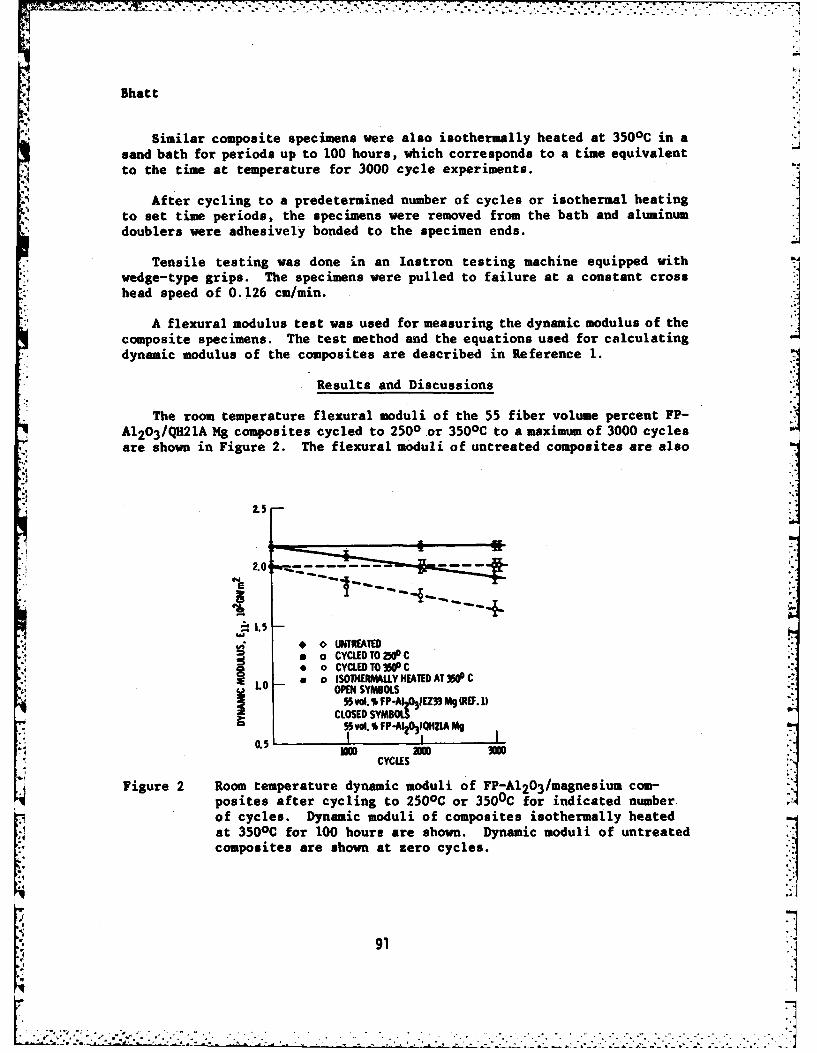
... . . . . .. *° . . . . • . 4 • 4 . .. 4 * * . % - . o° % • . • , . -.
hatt
Similar composite specimens were also isothermally heated at 350 0C in asand bath for periods up to 100 hours, which corresponds to a time equivalentto the time at temperature for 3000 cycle experiments.
After cycling to a predetermined number of cycles or isothermal heatingto set time periods, the specimens were removed from the bath and aluminumdoublers were adhesively bonded to the specimen ends.
Tensile testing was done in an Instron testing machine equipped withwedge-type grips. The specimens were pulled to failure at a constant cross
* head speed of 0.126 cm/mmn.
A flexural modulus test was used for measuring the dynamic modulus of the
composite specimens. The test method and the equations used for calculating
dynamic modulus of the composites are described in Reference 1.
Results and Discussions
The room temperature flexural moduli of the 55 fiber volume percent FP-A1203 /QH21A Mg composites cycled to 2500 or 350
0C to a maximum of 3000 cycles, are shown in Figure 2. The flexural moduli of untreated composites are also
L5 -
L 15
o o CYCLED TO 0 C•o CYCL.ED TO 3W C
o ISO1HERMALLY HEATED AT 30 C10 OPEN SYMBOLS
55Vol. S FP-AI -031EZ33 Mg (REF. 1) '~CLOSED SYMBOL
Posit5S~i afe F P.AIZOIQHZIA Mg, l~gO CYCLES
Figure 2 Room temperature dynamic moduli of FP-A1203/magnesium com-posites after cycling to 250 0C or 350 0C for indicated number.
of cycles. Dynamic moduli of composites isothermally heatedat 3500C for 100 hours are shown. Dynamic moduli of untreatedcomposites are shown at zero cycles.
91
4, I
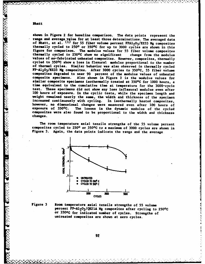
Bhatt
shown in Figure 2 for baseline comparison. The data points represent therange and average velue for at least three determinations. The averaged dataof Shatt, et al. (Ii for 55 fiber volume percent FPA120 3/EZ33 Hg compositesthermally cycled to 2500 or 3500C for up to 3000 cycles are shown in thisfigure for comparison. The modulus values for 55 fiber volume compositesthermally cycled to 250C show no significant change from the modulusvalues of as-fabricated unheated composites. However, composites, thermallycycled to 3500C show a loss in flexural modulus proportional to the numberof thermal cycles. Similar behavior was also observed in thermally cycledFP-A1203/KZ33 Hg composites. After 3000 cycles to 3500C, 55 fiber volumecomposites degraded to near 90 percent of the modulus values of unheatedcomposite specimens. Also shown in Figure 2 is the modulus values forsimilar composite specimens isothermally treated at 350 0C for 1000 hours, atime equivalent to the cumulative time at temperature for the 3000-cycletest. These specimens did not show any loss inflexural modulus even after100 hours of exposure. In the cyclic tests, while the specimen length andweight remained nearly the same, the width and thickness of the specimenincreased continuously with cycling. In isothermally heated composites,however, no dimensional changes were measured even after 100 hours ofexposure of 350 0C. The losses in the dynamic modulus of the cycledcomposites were also found to be proportional to the width and thicknesschanges.
The room temperature axial tensile strengths of the 55 volume percentcomposites cycled to 2500 or 350 0C to a maximum of 3000 cycles are shown inFigure 3. Again, the data points indicate the range and the average
.5
!4g4
*CYCLED TO 2W'C* CYCLED 10 3W C
.2I I
CYCLES
Figure 3 Room temperature axial tensile strengths of 55 volumepercent FP-A1203/QH21A Mg composites after cycling to 250 0Cor 3500c for indicated number of cycles. Strengths ofuntreated composites are shown at zero cycles.
92
. . .a.°
.
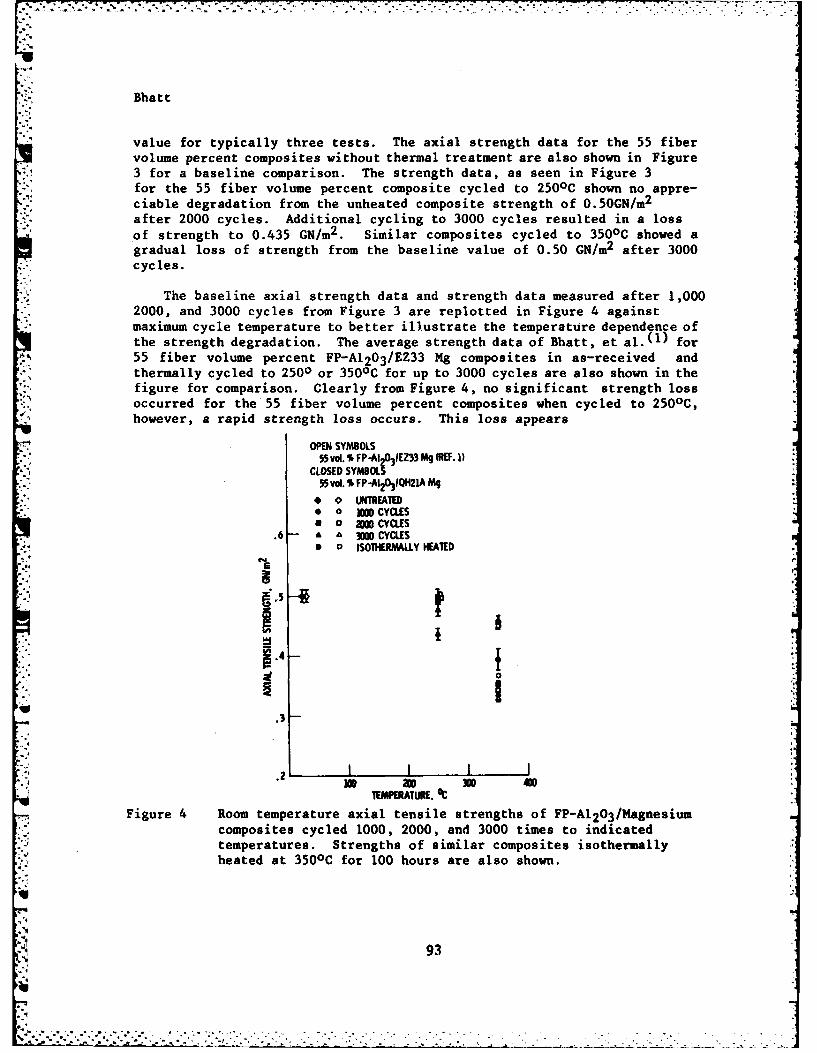
Bhatt
value for typically three tests. The axial strength data for the 55 fibervolume percent composites without thermal treatment are also shown in Figure3 for a baseline comparison. The strength data, as seen in Figure 3for the 55 fiber volume percent composite cycled to 250 0C shown no appre-ciable degradation from the unheated composite strength of 0.50GN/m
2
after 2000 cycles. Additional cycling to 3000 cycles resulted in a lossof strength to 0.435 GN/m 2 . Similar composites cycled to 3500 C showed agradual loss of strength from the baseline value of 0.50 GN/m 2 after 3000cycles.
The baseline axial strength data and strength data measured after 1,0002000, and 3000 cycles from Figure 3 are replotted in Figure 4 againstmaximum cycle temperature to better illustrate the temperature dependence ofthe strength degradation. The average strength data of Bhatt, et al.(l) for55 fiber volume percent FP-A1203/EZ33 Mg composites in as-received andthermally cycled to 2500 or 350 0C for up to 3000 cycles are also shown in thefigure for comparison. Clearly from Figure 4, no significant strength lossoccurred for the 55 fiber volume percent composites when cycled to 250 0C,however, a rapid strength loss occurs. This loss appears
OPEN SYMBOLS55vol %FP-AI2031EZ33 Mg (REF.1)
CLOSED SYMBOLiS55voI. % FP-AI2031QH2A Mq- * UNTREATED' 0 CYCLES9 a a~uCYCLES
.6 • 3000 CYCLESS D ISOTHERMALLY HEATED
.2.
. .I I I I
TEMPERATURE. OCFigure 4 Room temperature axial tensile strengths of FP-A1203/Magnesium
composites cycled 1000, 2000, and 3000 times to indicatedtemperatures. Strengths of similar composites isothermallyheated at 3500 C for 100 hours are also shown.
93
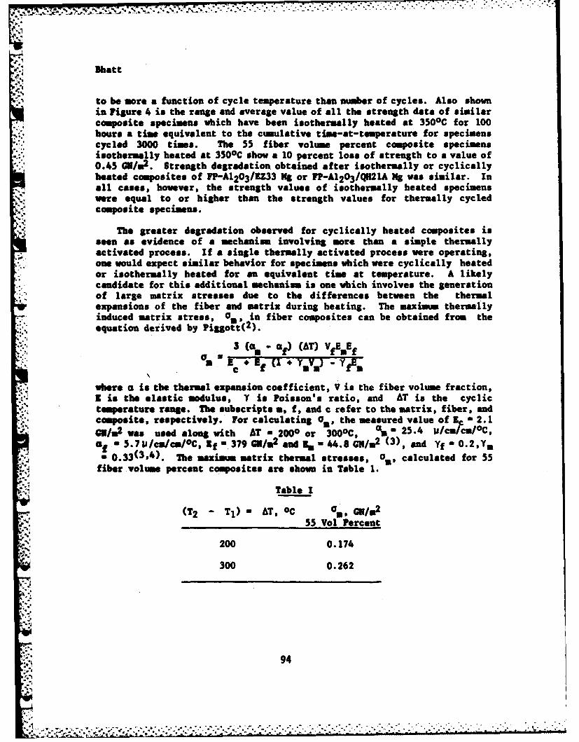
,hatt
to be more a function of cycle temperature than awmber of cycles. Also shownin Figure 4 is the range and average value of all the strength data of similarcomposite specimens which have been isothermally heated at 3500C for 100hours a time equivalent to the cumulative time-at-temperature for specimenscycled 3000 times. The 55 fiber volume percent composite specimensisothermally heated at 3500C show a 10 percent lose of strength to a value of0.45 GN/i 2 . Strength degradation obtained after isothermally or cyclicallyheated composites of FP-A1203/ZZ33 Mg or FP-A1203/QH21A Ng was similar. Inall cases, however, the strength values of isothermally heated specimenswere equal to or higher than the strength values for thermally cycled
'. , composite specimens.
The greater degradation observed for cyclically heated composites isseen as evidence of a mechanism involving more than a simple thermallyactivated process. If a single thermally activated process were operating,one would expect similar behavior for specimens which were cyclically heatedor isothermally heated for an equivalent time at temperature. A likelycandidate for this additional mechanism is one which involves the generationof large matrix stresses due to the differences between the thermalexpansions of the fiber and matrix during heating. The maximunm thermallyinduced matrix stress, o, in fiber composites can be obtained from theequation derived by Piggott(2 ).
3 m N -of) (AT) VfE mEf,, on "k € ' Ef a1 & m } -Y
were a is the thermal expansion coefficient, V is the fiber volume fraction,I is the elastic modulus, Y is Poisson's ratio, and AT is the cyclictemperature range. The subscripts u, f, and c refer to the matrix, fiber, andcomposite, respectively. For calculating G. , the measured value of a 2. 1GN/m2 was used along with AT - 2000 or 3000 C, %m - 25.4 jilmeTl/c,o - 5.7/cn/cm/oC, If= 379 G/m 2 and R. 44.8 GN/m 2 (3), and Yf - 0.2,Ym
3- 0. 4 ). The maximum matrix thermal stresses, o , calculated for 55fiber volume percent composites are shown in Table 1.
Table I
(T2 - T1)" AT, oC a., G/i 2
55 Vol Percent
200 0.174
300 0.262
.4.
94
............................... . ... .. ....
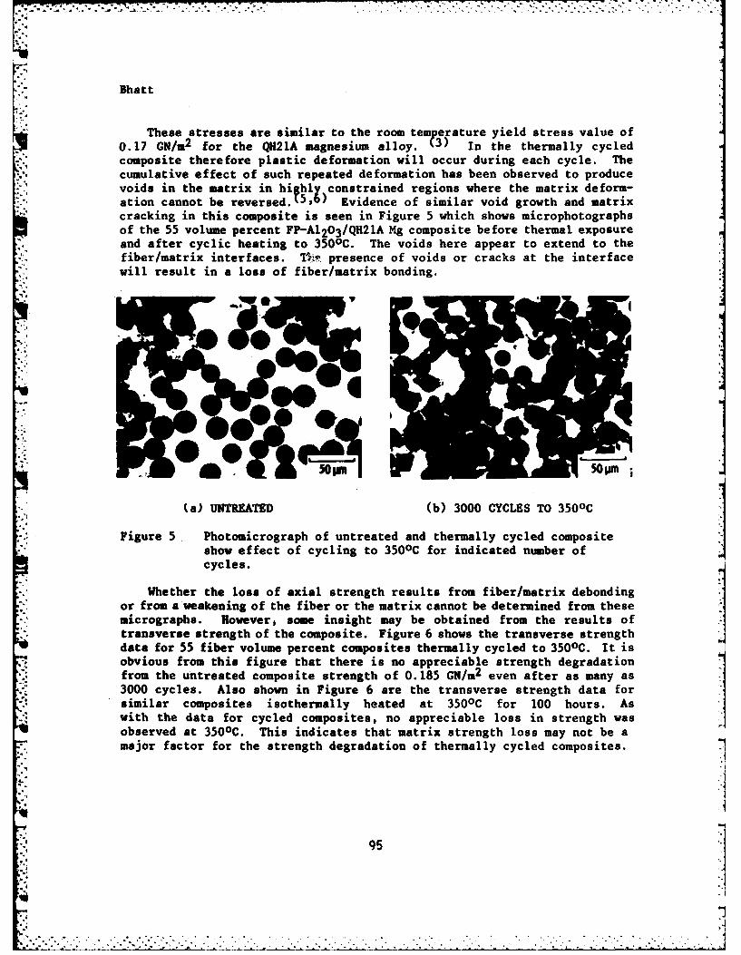
* ,-.a, . ,,,-.s . ' . :. -, .. ... . i' i~-i - . . ...- I -, i- .: ='. '- i -: - -
Bhatt
These stresses are similar to the room temperature yield stress value of0.17 GN/m2 for the QH21A magnesium alloy. ( In the thermally cycled
* composite therefore plastic deformation will occur during each cycle. Thecumulative effect of such repeated deformation has been observed to produce
1voids in the matrix in hihl constrained regions where the matrix deform-ation cannot be reversed." , ) Evidence of similar void growth and matrixcracking in this composite is seen in Figure 5 which shows microphotographsof the 55 volume percent FP-A1203/QH21A Mg composite before thermal exposureand after cyclic heating to 3500C. The voids here appear to extend to thefiber/matrix interfaces. Tiptj presence of voids or cracks at the interfacewill result in a loss of fiber/matrix bonding.
(a) UNTREATED (b) 3000 CYCLES TO 350 0C
Figure 5 Photomicrograph of untreated and thermally cycled compositeshow effect of cycling to 350 0C for indicated number ofcycles.
Whether the loss of axial strength results from fiber/matrix debondingor from a weakening of the fiber or the matrix cannot be determined from thesemicrographs. However, some insight may be obtained from the results oftransverse strength of the composite. Figure 6 shows the transverse strengthdata for 55 fiber volume percent composites thermally cycled to 3500C. It isobvious from this figure that there is no appreciable strength degradationfrom the untreated composite strength of 0.185 GN/m2 even after as many as3000 cycles. Also shown in Figure 6 are the transverse strength data for
,.similar composites isothermally heated at 350 0C for 100 hours. Aswith the data for cycled composites, no appreciable loss in strength wasobserved at 3500C. This indicates that matrix strength loss may not be amajor factor for the strength degradation of thermally cycled composites.
* 95
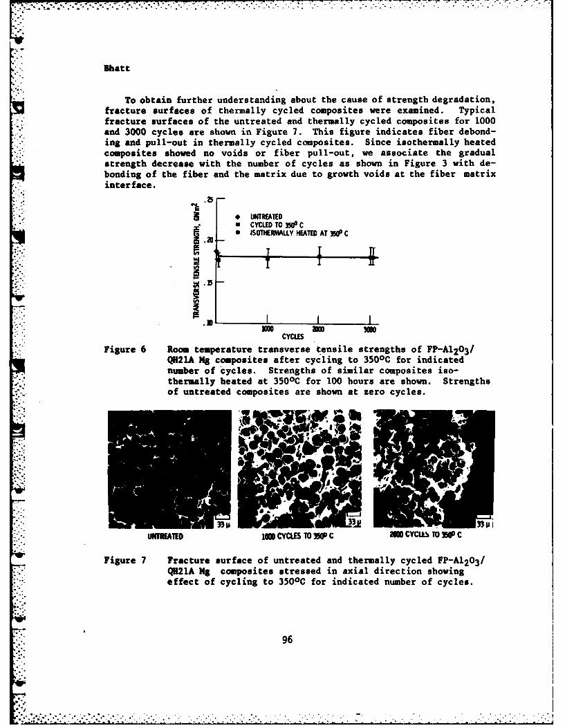
Bhatt
To obtain further understanding about the cause of strength degradation,fracture surfaces of thermally cycled composites were examined. Typicalfracture surfaces of the untreated and thermally cycled composites for 1000and 3000 cycles are shown in Figure 7. This figure indicates fiber debond-ing and pull-out in thermally cycled composites. Since isothermally heatedcomposites showed no voids or fiber pull-out, we associate the gradualstrength decrease with the number of cycles as shown in Figure 3 with de-bonding of the fiber and the matrix due to growth voids at the fiber matrixinterface.
UNTREATED•CYCLED TO YAO0°
. ISOTHERMALLY HEATED AT 350 C.20-
S.15
.mI I I
CYCLESFigure 6 Room temperature transverse tensile strengths of FP-A1203/
QH21A Mg composites after cycling to 3500C for indicatednumber of cycles. Strengths of similar composites iso-thermally heated at 3500C for 100 hours are shown. Strengthsof untreated composites are shown at zero cycles.
UNnREATED 100 CYCLES TO 3W C MN CYCLB TO 3Wo C
Figure 7 Fracture surface of untreated and thermally cycled FP-A1203 /Q921A Mg composites stressed in axial direction showingeffect of cycling to 350 0C for indicated number of cycles.
96
li- ,- '; ,;:.- ,- ', '. ', '.' .- .- ', , ' . " - ' , : - '. '. .- . . .- " . ' ' " . " . .' - . . ' ,' ',- ,- -- .- '-
Bhatt
Susumar)
The effects of cyclic and isothermal heat treatments on the axial andtransverse tensile strength and axial moduli of 55 volume percent FP-A1203/QH21A Mg composites have been evaluated to understand the cause of thermallyinduced strength degradation and to help determine the limiting use con-ditions for these composites. Specific findings are as follows:
1. Thermal cycling of FP-A1 2 03 /QH21A Mg composites to 250 0 C for 2000cycles did not cause any appreciable room temperature strength or modulusloss compared with baseline data for untreated composites. In contrast,
*. composites thermally cycled to 3500 C showed considerable loss in both axialstrength and modulus. No appreciable loss in room temperature transversetensile strength of composites was measured after thermal cycling.
2. Measurement of the transverse strength and fractographic analysis ofthermally cycled composites indicated interface void formation and matrixcracking and fiber debonding as prime contributors to observed strength andmodulus losses. These results are consistent with degradation mechanismbased on thermal-induced stresses in the matrix.
3. No appreciable loss in the axial dynamic modulus of these compositeswas observed after isothermal exposure. Small strength losses observed inisothermally heated composites were attributed to matrix softening.
4. The high temperature mechanical properties were not measured for thecomposites in this study. This would be required to properly design usingFP-A1 2 0 3 /QH21A composites. However, aside from the usual matrix softeningat higher temperatures, this study indicates that we would not expectadditional axial strength or modulus degradation resulting from eitherisothermal or cyclic exposure below 2000 cycles or 2500C.
97
' - ;': r" ,:. /",, - :' : '-. ;: ::: :;: : ::,::.....................................-...........-..-..-....-".,.....-..:i :
Bhatt
References
(1) Bhatt, R. T. and Grimes, H. H., "Thermal Degradation of the TensileProperties of Unidirectionally Reinforced FP-A1203/EZ33 Mg Compos-ities," NASA TM-82817, 1982.
(2) Piggott, M. R., "Load Bearing Fiber Composites," pp. 208, PergamonPress, Oxford, NY, 1980.
(3) Metals Handbook, Vol. I, "Properties and Selection of Metals," Ameri-can Society for Metals, Metals Park, OH, 1961.
(4) Bacon, J. F., Prewo, K. M., and Veltri, R. D., "Glass Matrix Compos-ities-II-Alumina Reinforced Glass," pp. 753-769, in Proceedings ofthe 1978 International Conference on Composite Materials, Noton, B.,Signorelli, R., Street, K., and Phillips, L., Editors, AIME, New York,NY, 1978.
(5) Shahinian, P., "Thermai Fatigue of Aluminum-Boron Composites," SANPEQuart., Vol. 2, 1970, pp. 28-35.
(6) Kim, W. H., Koczak, M. J., and Lawley, A., "Effects of Isothermal andCyclic Exposures on Interface Structure and Mechanical Properties ofFP -A1203/Aluminum Composites," New Developments and Applications inComposites, Doris Kuhlmann-Wildorf and W. C. Harrigan, Editors, Pro-ceedings of a Symposium sponsored by the TMS-AIME Physical Metallurgyand Composites, 1979, pp. 40-53.
98
.. . ........ .... .. ... .................. . ..
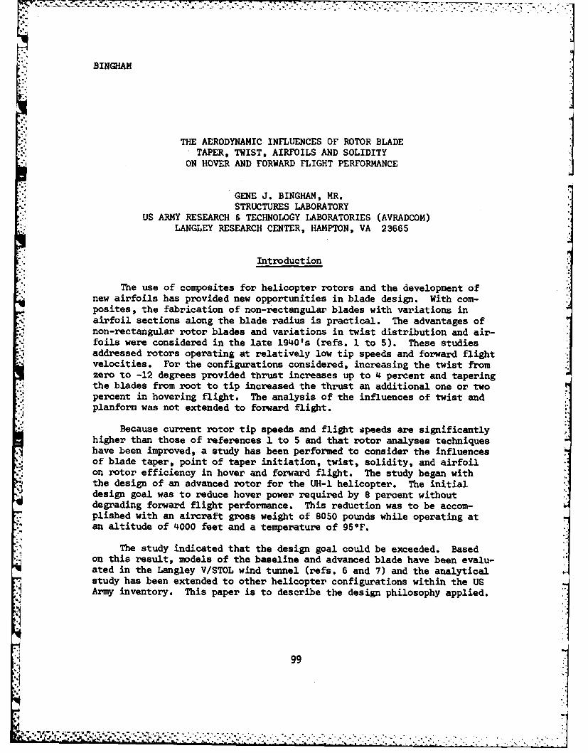
BINGHAM
THE AERODYNAMIC INFLUENCES OF ROTOR BLADETAPER, TWIST, AIRFOILS AND SOLIDITY
ON HOVER AND FORWARD FLIGHT PERFORMANCE
GENE J. BINGHAM, MR.STRUCTURES LABORATORY
US ARMY RESEARCH & TECHNOLOGY LABORATORIES (AVRADCOM)LANGLEY RESEARCH CENTER, HAMPTON, VA 23665
Intro duct ion
The use of composites for helicopter rotors and the development ofnew airfoils has provided new opportunities in blade design. With com-posites, the fabrication of non-rectangular blades with variations inairfoil sections along the blade radius is practical. The advantages ofnon-rectangular rotor blades and variations in twist distribution and air-foils were considered in the late 1940's (refs. 1 to 5). These studiesaddressed rotors operating at relatively low tip speeds and forward flightvelocities. For the configurations considered, increasing the twist fromzero to -12 degrees provided thrust increases up to 4 percent and taperingthe blades from root to tip increased the thrust an additional one or twopercent in hovering flight. The analysis of the influences of twist andplanform was not extended to forward flight.
Because current rotor tip speeds and flight speeds are significantlyhigher than those of references 1 to 5 and that rotor analyses techniqueshave been improved, a study has been performed to consider the influencesof blade taper, point of taper initiation, twist, solidity, and airfoilon rotor efficiency in hover and forward flight. The study began withthe design of an advanced rotor for the UH-I helicopter. The initialdesign goal was to reduce hover power required by 8 percent withoutdegrading forward flight performance. This reduction was to be accom-plished with an aircraft gross weight of 8050 pounds while operating atan altitude of 4000 feet and a temperature of 959F.
The study indicated that the design goal could be exceeded. Basedon this result, models of the baseline and advanced blade have been evalu-ated in the Langley V/STOL wind tunnel (refs. 6 and 7) and the analyticalstudy has been extended to other helicopter configurations within the USArmy inventory. This paper is to describe the design philosophy applied.
[99
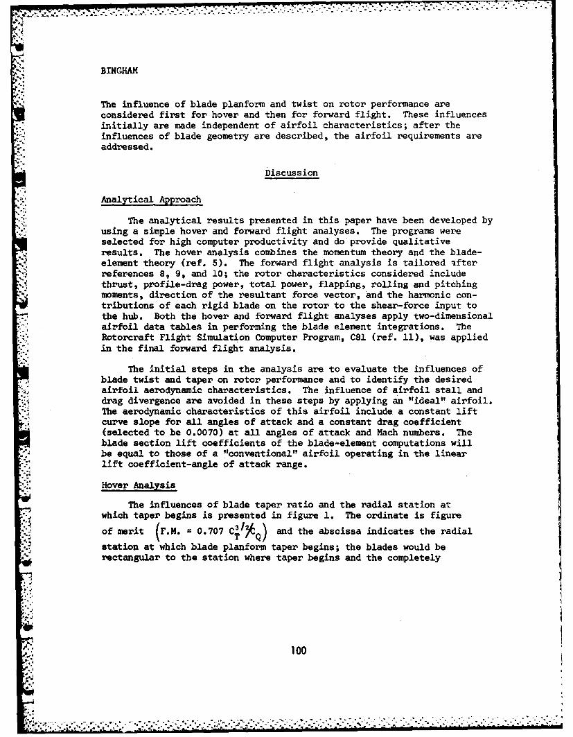
BINGHAM
The influence of blade planform and twist on rotor performance areconsidered first for hover and then for forward flight. These influencesinitially are made independent of airfoil characteristics; after the
V influences of blade geometry are described, the airfoil requirements areaddressed.
Discussion
Analytical Approach
The analytical results presented in this paper have been developed byusing a simple hover and forward flight analyses. The programs wereselected for high computer productivity and do provide qualitativeresults. The hover analysis combines the momentum theory and the blade-element theory (ref. 5). The forward flight analysis is tailored lfterreferences 8, 9, and 10; the rotor characteristics considered includethrust, profile-drag power, total power, flapping, rolling and pitchingmoments, direction of the resultant force vector, and the harmonic con-tributions of each rigid blade on the rotor to the shear-force input tothe hub. Both the hover and forward flight analyses apply two-dimensionalairfoil data tables in performing the blade element integrations. TheRotorcraft Flight Simulation Computer Program, C81 (ref. 11), was appliedin the final forward flight analysis.
The initial steps in the analysis are to evaluate the influences ofblade twist and taper on rotor performance and to identify the desiredairfoil aerodynamic characteristics. The influence of airfoil stall anddrag divergence are avoided in these steps by applying an "ideal" airfoil.The aerodynamic characteristics of this airfoil include a constant liftcurve slope for all angles of attack and a constant drag coefficient(selected to be 0.0070) at all angles of attack and Mach numbers. Theblade section lift coefficients of the blade-element computations willbe equal to those of a "conventional" airfoil operating in the linearlift coefficient-angle of attack range.
Hover Analysis
The influences of blade taper ratio and the radial station atwhich taper begins is presented in figure 1 The ordinate is figure
of merit F.M. = 0.707 C31 and the abscissa indicates the radial
station at which blade planform taper begins; the blades would berectangular to the station where taper begins and the completely
A.i 100
-- .".: *" "*"' ''*''''' ,''" ;,.:'''. . ' ' "'' ,; ." "' " "" " "' ' " / ': ' "" " "' i" ", -" "" " .-' .
9t' " i *.-- I i -*i ia *
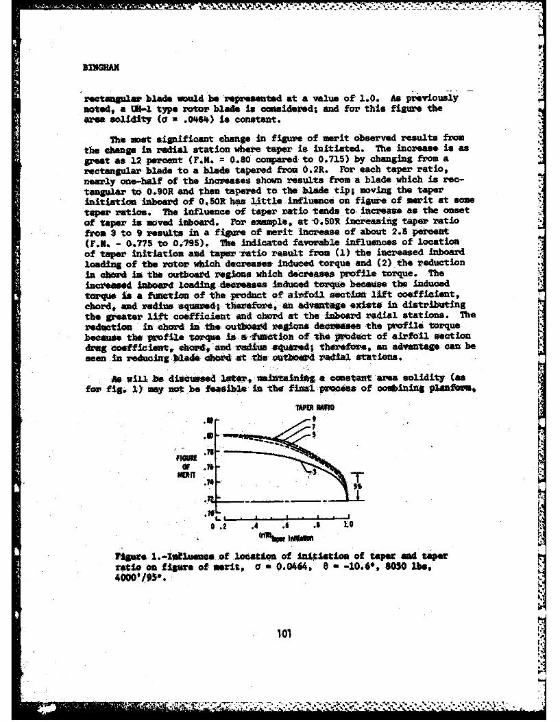
rectangular blade would be epeeedat a value of 1.0. As previouslynoted, a M-11 type rotor blade is considered; and for this figure thearea solidity (Co .044) is constant.
The most significant change In figure of merit observed results from t
the duange In radial station where taper is initiated. The increase is asgreat as 12 percent (F.M. = 0.80 compared to 0.715) by changing from arectangular blade to a blade tapered from 0.*2R. For each taper ratio,newly one-half of the increases shown results from a blade which is rec-tangular to 0.40R and then tapered to the blade tip; moving the taperinitiation Inboard of 0. 5OR has little -influence on figure of merit at sometaper ratios,, The influence of taper ratio tends to-increase as the onsetof taper In moved inboard. , For example, at V0 * 5R increasing taper ratiofrom 3 to 9 resul.ts In a figure of merit increase of about 2.6 percent(F.K. - 0.775 to 0.195). The indicated favorable influences of locationof taper initiation and taper -ratio result fromi (1) the increased inadloading of the rotor which decreases induced torque and (2) the reductionIn chord in the outboard regimne which decreases profile torque.* Theincreased inboard loading-decreases induced torque because the inducedtorque $& a fusotion of the product of airfoil section lift coefficient,chord * and radius squared; therefore, an advantage exists in distributingthe greater lift coefficient and -chord at the inboard radial stations.* Theredaction in chord In the outboard regions, deocreases the profile torquebecause the profile torque its *-fftwot ion of the product of airfoil sectiondrag: coofficient, chord, and redii squared; therefoe, an advantage can beseen in reducing blade chord at the outboard radial stations.
Aswill be discussed later, mivtaining a constant area solidity (asfor fig. 1) say not be fleasible in, the final VPwocss of cosbining plmnfoum,
FlowtOF A-1
WRIT
0.2 .4 .6 . 0
?Sgte .-Iluee. f lcatonof ftietlon of tape and taperratio or, figure of meit, a -0.0464, 6 -l0.6, 8050 lb.,
1011
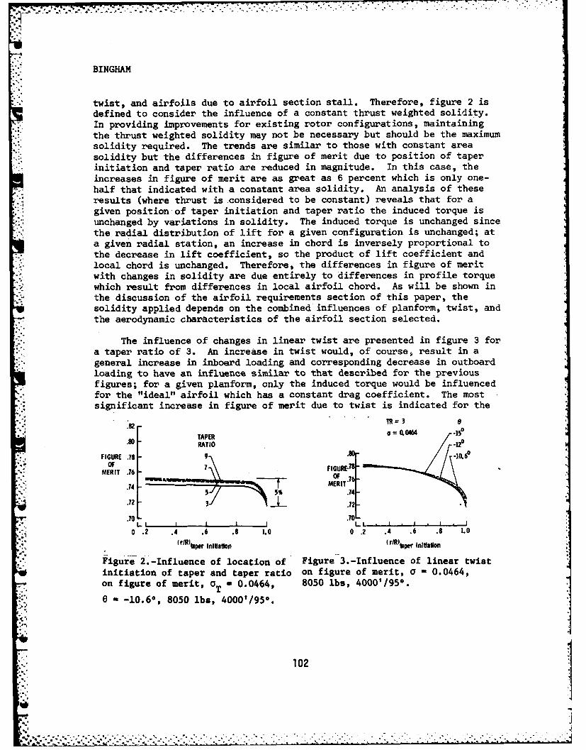
BINGHAM
twist, and airfoils due to airfoil section stall. Therefore, figure 2 isdefined to consider the influence of a constant thrust weighted solidity.In providing improvements for existing rotor configurations, maintainingthe thrust weighted solidity may not be necessary but should be the maximumsolidity required. The trends are similar to those with constant area
.. solidity but the differences in figure of merit due to position of taperinitiation and taper ratio are reduced in magnitude. In this case, theincreases in figure of merit are as great as 6 percent which is only one-half that indicated with a constant area solidity. An analysis of theseresults (where thrust is considered to be constant) reveals that for agiven position of taper initiation and taper ratio the induced torque isunchanged by variations in solidity. The induced torque is unchanged sincethe radial distribution of lift for a given configuration is unchanged; ata given radial station, an increase in chord is inversely proportional tothe decrease in lift coefficient, so the product of lift coefficient andlocal chord is unchanged. Therefore, the differences in figure of meritwith changes in solidity are due entirely to differences in profile torquewhich result from differences in local airfoil chord. As will be shown inthe discussion of the airfoil requirements section of this paper, thesolidity applied depends on the combined influences of planform, twist, andthe aerodynamic characteristics of the airfoil section selected.
The influence of changes in linear twist are presented in figure 3 fora taper ratio of 3. An increase in twist would, of course, result in ageneral increase in inboard loading and corresponding decrease in outboardloading to have an influence similar to that described for the previousfigures; for a given planform, only the induced torque would be influencedfor the "ideal" airfoil which has a constant drag coefficient. The mostsignificant increase in figure of merit due to twist is indicated for the
-~.82 -T
* TAPER -05.0-RATIO -120
FIGURE .78 9 • -10.60MERIT .76 7FIGURE
OF t6.74 -MER IT.__ .74-.72 ,.70 " 7°0-
" , I I I I I L , n . I , i I
0 .2 .4 .6 .8 1.0 0 .2 .4 .6 .8 L.0
(rIRi pr InIhation (rlR~hper InItatlon
Figure 2.-Influence of location of Figure 3.-Influence of linear twistinitiation of taper and taper ratio on figure of merit, a = 0.0464,on figure of merit, a a 0.0464, 8050 lbs, 4000'/950.
" " -10.60, 8050 lbs, 40001/950.
102

BINGHAM
rectangular planform (r/R 1.0); the increase in twist from -10.6 ° to -15°
increases the figure of merit about 2 percent. As the taper initiationposition is moved inboard, the influence of increased twist is reduced.
Forward Flight Analysis
The influence of blade taper and the radial station at which taper isinitiated on forward flight performance is indicated in figure 4. Theordinate is torque coefficient and the abscissa again defines the radialposition where taper is initiated. The forward flight velocity consideredis 110 knots (near maximum for the UH-I in level flight); the area solidityis constant, inflow is uniform, and the other parameters are the same asthose for figure 1. Similar to the case for hover, a significant change intorque coefficient results from changes in radial station where taper isinitiated; the decrease is as great as 16 percent by initiating taper at0.2R. Unlike the previously discussed case for hover (fig. 1), only asmall part of the total decrease results from changing the blade from fullyrectangular to a configuration with taper initiated at 0.9R and the advan-tage of moving the taper initiation location inboard of 0.SR is greater inforward flight than in hover. As for the hover case, increases in taperratio from 3 to 9 provide several percent decreases in torque coefficient.
" The favorable influences are due to the inboard loading and the reductionin chord in the outboard regions.
The results of the forward flight analysis with constant thrustweighted solidity are presented in figure 5. As for hover, the increased
.13 X 103 3 TR.1 1 3
.13 -X10 35- -F
.12 -TR .12TORQUE 3 TORQUE 91
COEFFICIENT 5 COEFFICIENT
S 7
.10 .10=" I I I I L I I I I I-
20 . .4 .6 .8 1.0 0 .2 .4 .6 .8 1.0r1R) topr InitlI&Wo (r/R) Oer Inltld.
Figure 4.-Influence of location of Figure 5.-Influence of location ofinitiation of taper and taper ratio initiation of taper and taper ratioon torque coefficient, 0 - 0.0464, on torque coefficient 0T - 0.0464,e - -10.60, .8050 lbs, 4000'/95 °,110 knots. 6 - -10.60 , 8050 ib8, 4000'/950 ,
110 knots.
103
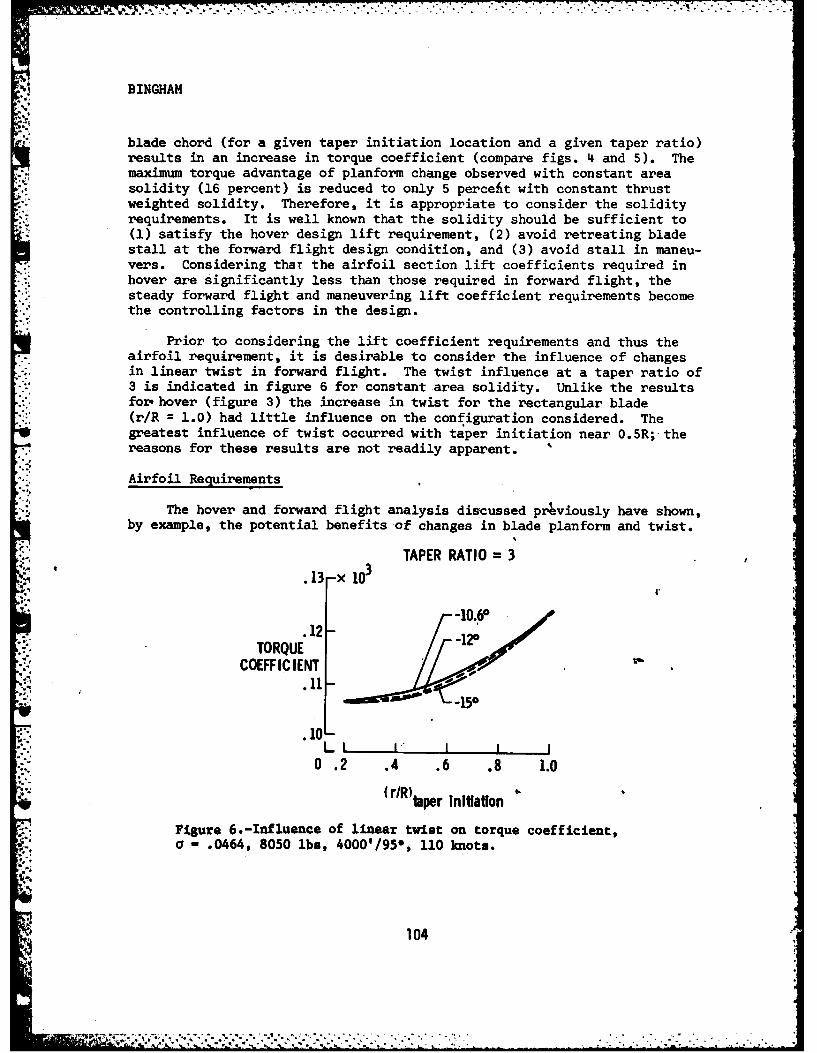
N! BINGHAM* ,1
blade chord (for a given taper initiation location and a given taper ratio)results in an increase in torque coefficient (compare figs. 4 and 5). Themaximum torque advantage of planform change observed with constant areasolidity (16 percent) is reduced to only 5 perceft with constant thrustweighted solidity. Therefore, it is appropriate to consider the solidityrequirements. It is well known that the solidity should be sufficient to(1) satisfy the hover design lift requirement, (2) avoid retreating bladestall at the forward flight design condition, and (3) avoid stall in maneu-vers. Considering that the airfoil section lift coefficients required inhover are significantly less than those required in forward flight, thesteady forward flight and maneuvering lift coefficient requirements becomethe controlling factors in the design.
Prior to considering the lift coefficient requirements and thus theairfoil requirement, it is desirable to consider the influence of changesin linear twist in forward flight. The twist influence at a taper ratio of3 is indicated in figure 6 for constant area solidity. Unlike the resultsfox hover (figure 3) the increase in twist for the rectangular blade(r/R = 1.0) had little influence on the configuration considered. Thegreatest influence of twist occurred with taper initiation near 0.5R; thereasons for these results are not readily apparent. "
*' Airfoil Requirements
The hover and forward flight analysis discussed previously have shown,by example, the potential benefits of changes in blade planform and twist.II
.13 -x1 TAPER RATIO =3
TORQUECOEFF IC lENT
.11 -~-150
.10LI I I I I
0 .2 .4 .6 .8 1.0
(rlR) taper Initiation
Figure 6.-Influence of linear twist on torque coefficient,a 0".0464, 8050 lb, 4000'/950, 110 knots.
104
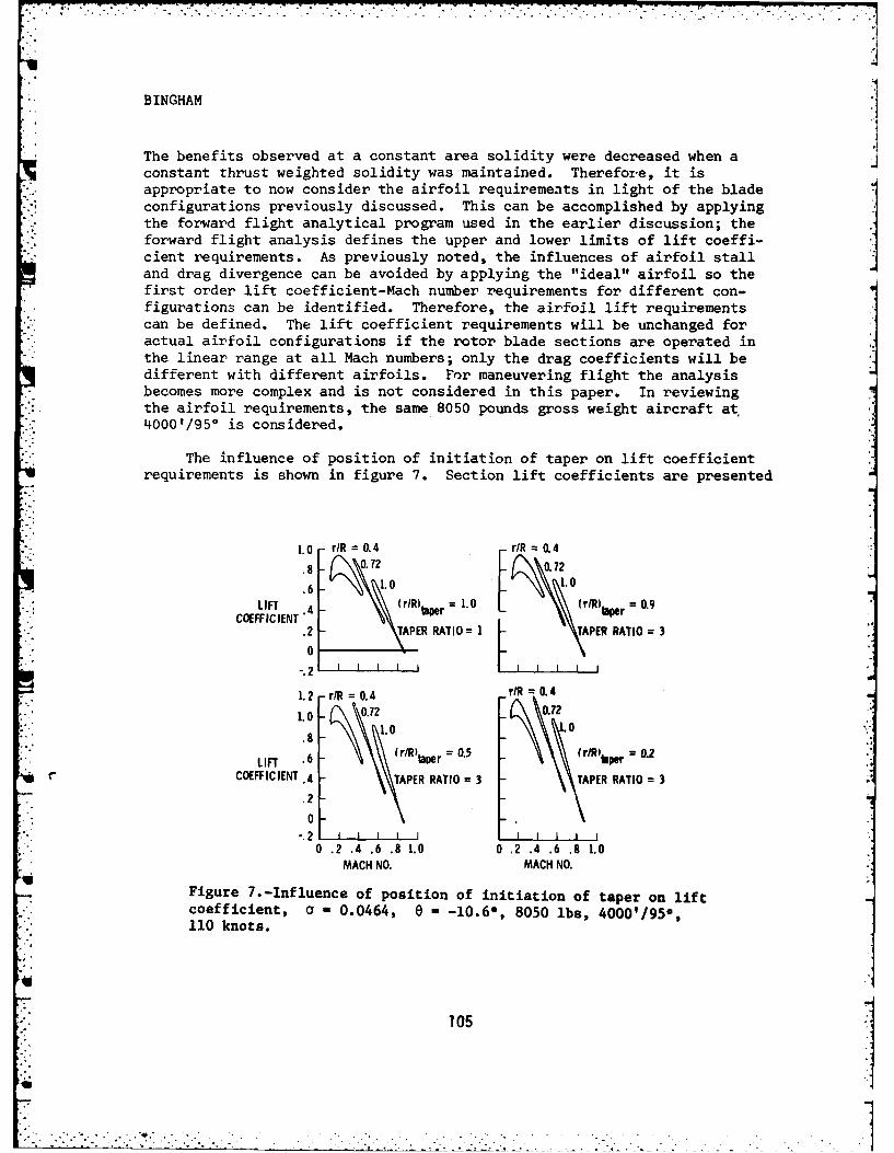
BINGHAM
The benefits observed at a constant area solidity were decreased when aconstant thrust weighted solidity was maintained. Therefore, it isappropriate to now consider the airfoil requirements in light of the bladeconfigurations previously discussed. This can be accomplished by applyingthe forward flight analytical program used in the earlier discussion; theforward flight analysis defines the upper and lower limits of lift coeffi-cient requirements. As previously noted, the influences of airfoil stalland drag divergence can be avoided by applying the "ideal" airfoil so thefirst order lift coefficient-Mach number requirements for different con-figurations can be identified. Therefore, the airfoil lift requirementscan be defined. The lift coefficient requirements will be unchanged foractual airfoil configurations if the rotor blade sections are operated inthe linear range at all Mach numbers; only the drag coefficients will bedifferent with different airfoils. For maneuvering flight the analysisbecomes more complex and is not considered in this paper. In reviewingthe airfoil requirements, the same 8050 pounds gross weight aircraft at,40001/95* is considered.
:. The influence of position of initiation of taper on lift coefficientrequirements is shown in figure 7. Section lift coefficients are presented
1.0 - rR 0= .4 r/R 0. 4
COEFFICIENT ..2 % TAPER RATIO= 1 TAPER RATIO = 30
-.2 _j
1.2 -rIR=0.4 _rIR 0.4
1.0 - 0.72 ~.721.0 L
LIFT .6 (rlR)b er = 0.5 _(r /Rlbpe 0.2
r COEFFICIENT .4 TAPER RATIO = 3 \TAPER RATIO = 3
.2
0-.2 _I
0 .2 .4 .6 .8 1.0 0 .2 .4 .6 .8 1.0MACH NO. MACH NO.
Figure 7.-Influence of position of initiation of taper on liftcoefficient, a - 0.0464, e - -l0.6, 8050 lbs, 4000'/95,110 knots.
105
"o1
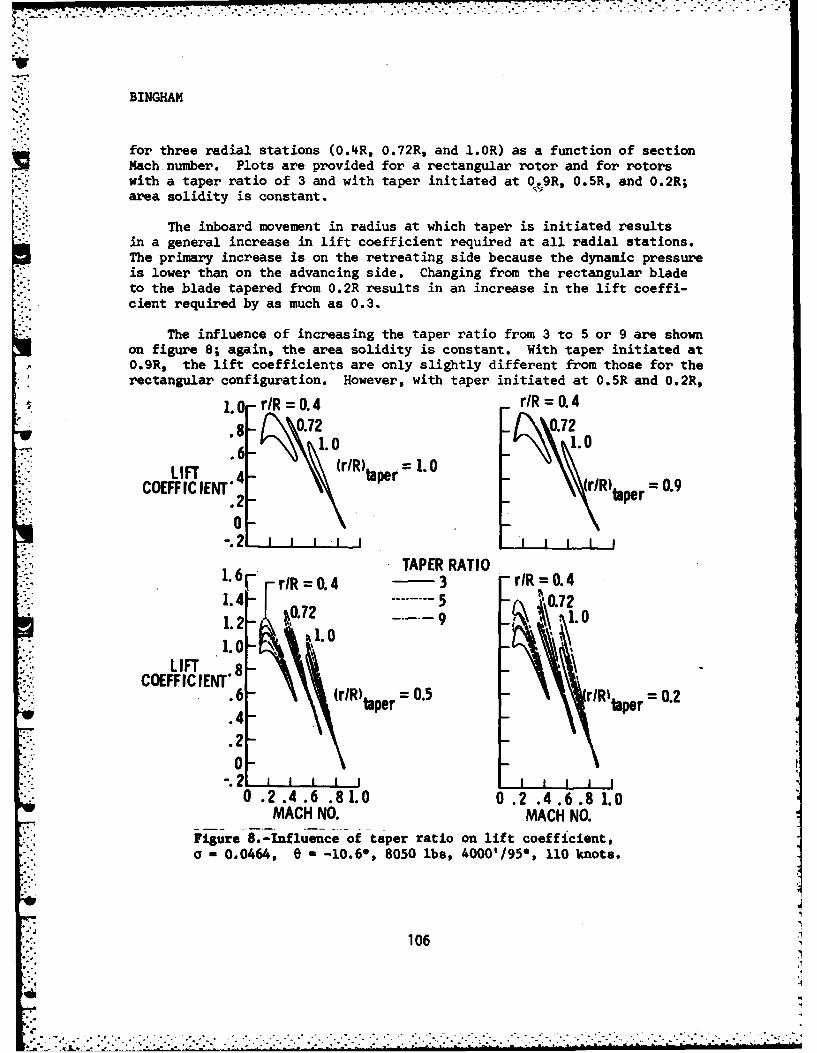
.-. ... . .
BINGHAM
for three radial stations (0.4R, 0.72R, and 1.OR) as a function of sectionMach number. Plots are provided for a rectangular rotor and for rotorswith a taper ratio of 3 and with taper initiated at 0.9R, 0.5R, and 0.2R;area solidity is constant.
The inboard movement in radius at which taper is initiated resultsin a general increase in lift coefficient required at all radial stations.The primary increase is on the retreating side because the dynamic pressureis lower than on the advancing side. Changing from the rectangular bladeto the blade tapered from 0.2R results in an increase in the lift coeffi-cient required by as much as 0.3.
The influence of increasing the taper ratio from 3 to 5 or 9 are shownon figure 8; again, the area solidity is constant. With taper initiated at0.R, the lift coefficients are only slightly different from those for therectangular configuration. However, with taper initiated at 0.5R and 0.2R,
1.0- r/R =0.4 rlR = 0.4W.8_ _/.72\o.72
LIFT : (r/R)ta 1.0\R pe =0.COEFFIC IENT tar =
.2-0
-. 2 L_____ _ , i1.6- TAPER RATIO--,rrR =0.4 - 3 rR =0.4
1.4 ------5031.21.4 ........ 9 0.:.1.0 005.0
LIFT 8COEFFIC IENT'
.6 (r/R)taper 0.5 r/R)taper 0.2
.4
.20 \
-.21a0 .2.4.6 .81.0 0.2 .4 .6.8 1.0
MACH NO. MACH NO.
Figure 8.-Influence of taper ratio on lift coefficient,, - 0.0464, e - -10.60, 8050 lbs, 4000'/95*, 110 knots.
106
.. -
.. .. . .. ... . .. . .. . .. . .. ,

BINGHAM
the increases in required lift coefficient are as large as those resultingfrom the changes in taper initiation observed in figure 7. It is ofinterest to note here, at l.OR, satisfying both a drag divergent Mach num-ber of 0.87 and a maximum lift coefficient near 1.3 for taper initiationat 0.2R is beyond the capability of known airfoil sections; also, it shouldbe noted that the position at which taper can be initiated and the blade
* taper ratio can be controlled by the maximum lift coefficients of theavailable airfoils.
As shown in figure 9, a reduction in the maximum lift requirement atthe blade tip (r/R = 1.0) can be accomplished by increasing the lineartwist of the blade. In the example shown, the increase is from -10.6 de-grees to -15 degrees. The tip section lift coefficients are decreased atall Mach numbers. At 0.72R the twist has little influence on the opera-tional lift coefficient. At 0.4R, the increased twist increases the in-board lift coefficients to result in an increase in inboard loading. Theincrease in twist results in requirements more consistent with current air-foil capability than those observed in figure 8 and permits adjustments inrequirements to match the maximum lift coefficients of available airfoils.
The influences of blade solidity on the lift coefficient are shown in
r =0.4 L rIR-.,.1. . 721..I 1 0.8 . '
LIFT .6 R 0.9COEFFIC IENT 2 6= -10.6o .4
0 0i
2 -.2F I I II ITAPER RATIO
d-, ;"14- - r/R = 0.41.6 R ---- 1.6-
1.4 %.72 9.. 9 1.4 V1.0 1.
", 1.2 9 1.4 2 i
LIFT 10 (I.0 1.0.2COEFFICIENT 1. r 0.2 1.
.6 .6
.4a-16 .4.2 .200-. -.0.2.4.6.81.0 0.2.4 .6.8 1.0
MACH NO. MACH NO.
Figure 9.-Influence of taper ratio and linear twist on liftcoefficient, a - 0.0464, 8 - -10.60, 8050 lbs, 4000'/950,110 knots.
107
-ILA.
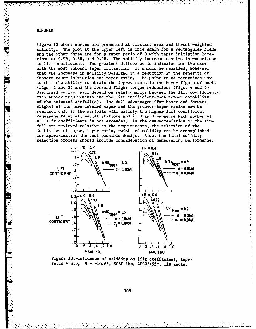
BINGHAM
figure 10 where curves are presented at constant area and thrust weightedsolidity. The plot at the upper left is once again for a rectangular bladeand the other three are for a taper ratio of 3 with taper initiation loca-tions at 0.9R, 0.5R, and 0.2R. The solidity increase results in reductionsin lift coefficient. The greatest difference is indicated for the casewith the most inboard taper initiation. It should be recalled, however,that the increase in solidity resulted in a reduction in the benefits ofinboard taper initiation and taper ratio. The point to be recognized nowis that the ability to obtain the improvements in the hover figure of merit(figs. 1 and 2) and the forward flight torque reductions (figs. 4 and 5)discussed earlier will depend on relationships between the lift coefficient-Mach number requirements and the lift coefficient-Mach number capabilityof the selected airfoil(s). The full advantages (for hover and forwardflight) of the more inboard taper and the greater taper ratios can berealized only if the airfoils will satisfy the higher lift coefficientrequirements at all radial stations and if drag divergence Mach number atall lift coefficients is not exceeded. As the characteristics of the air-foil are reviewed relative to the requirements, the selection of theinitiation of taper, taper ratio, twist and solidity can be accomplishedfor approximating the best possible design. Also, the final solidityselection process should include consideration of maneuvering performance.
rR =O.4 rR =0.41.8
' , ,--, 0.72 -,- 0.72
.6 (rRtaper= 1.0 (rRItaer = 0.9
LIFT 4- - 0.0464 a = 0.04M"- COEFFICIENT ------ OT = 0.04M4.2. - _
0
1 - r/R 0. 4 rlR 0.4
10 0.72.07:. -. 0 1.0?k ,\%"8/ 1.0 (rlR p =0.2
V \\ (r/R)te 0.5 taper,,,,_,.
LIFT .6 rl o = ._ 0.0464COEFFICIENT .4- - =0.0464 - "
.2-
0-
0 .2 .4 .6 .8 1.0 0 .2 .4 .6 .8 1.0MACH NO. MACH NO.
* Figure 1O.-Influence of solidity on lift coefficient, taperratio - 3.0, 6 - -10.6, 8050 Ibs, 4000'/950, 110 knots.
108
_Ei .............. :.:. ,... . .. .. .: . .< - ::::::;: . : . :; , . ,: : . .: - . - .
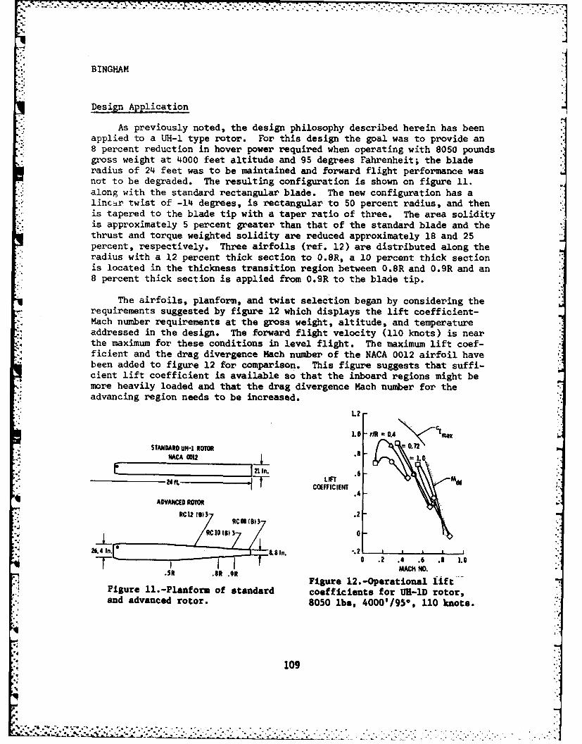
BINGHAM
Design Application
As previously noted, the design philosophy described herein has beenapplied to a UH-l type rotor. For this design the goal was to provide an8 percent reduction in hover power required when operating with 8050 poundsgross weight at 4000 feet altitude and 95 degrees Fahrenheit; the bladeradius of 24 feet was to be maintained and forward flight performance wasnot to be degraded. The resulting configuration is shown on figure 11.along with the standard rectangular blade. The new configuration has alincar twist of -14 degrees, is rectangular to 50 percent radius, and thenis tapered to the blade tip with a taper ratio of three. The area solidityis approximately 5 percent greater than that of the standard blade and thethrust and torque weighted solidity are reduced approximately 18 and 25percent, respectively. Three airfoils (ref. 12) are distributed along theradius with a 12 percent thick section to 0.8R, a 10 percent thick sectionis located in the thickness transition region between 0.8R and 0.9R and an
*i 8 percent thick section is applied from 0.9R to the blade tip.
The airfoils, planform, and twist selection began by considering therequirements suggested by figure 12 which displays the lift coefficient-
%. Mach number requirements at the gross weight, altitude, and temperatureaddressed in the design. The forward flight velocity (110 knots) is nearthe maximum for these conditions in level flight. The maximum lift coef-ficient and the drag divergence Mach number of the NACA 0012 airfoil havebeen added to figure 12 for comparison. This figure suggests that suffi-cient lift coefficient is available so that the inboard regions might bemore heavily loaded and that the drag divergence Mach number for theadvancing region needs to be increased.
L2
LO- rR U 0.mxSTANDARD UH-I ROTOR 0.72
NACA 0012 1.
~ LIFTCOEFFICIENT
.4
-
ADVANCED ROTOR -
RCI2 ()3)- .2RCM (1113
RC 10(5) 30
26.4 In. 8 In. ;2 I
I I 0 .2 .4 .6 .8 1.0T. 81I 91I MACH NO.. .SR .SR .9R
Figure 12.-Operational lift'Figure ll.-Planform of standard coefficients for UK-iD rotor,and advanced rotor. 8050 ibs, 4000'/950, 110 knots.
II1,
.I1 9"
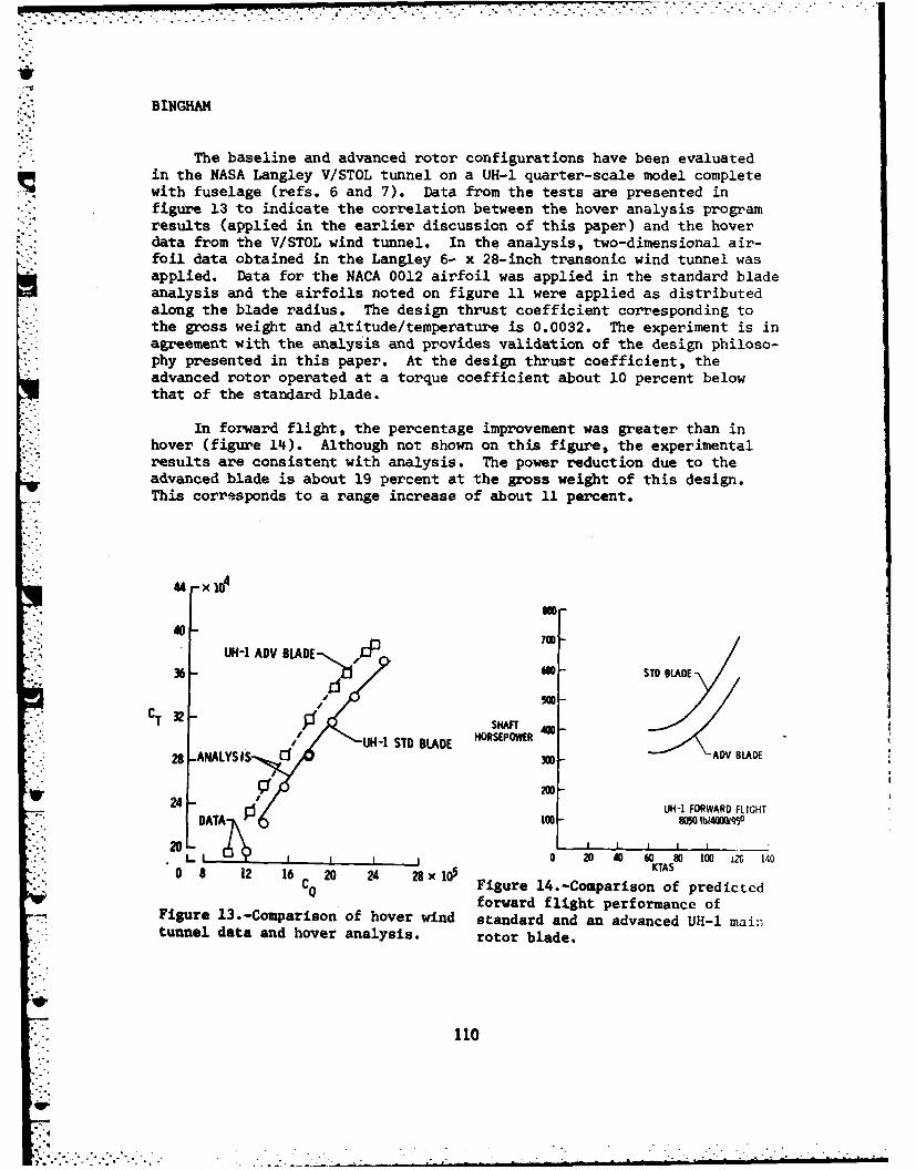
BINGHAM
The baseline and advanced rotor configurations have been evaluatedin the NASA Langley V/STOL tunnel on a UH-l quarter-scale model completewith fuselage (refs. 6 and 7). Data from the tests are presented infigure 13 to indicate the correlation between the hover analysis programresults (applied in the earlier discussion of this paper) and the hoverdata from the V/STOL wind tunnel. In the analysis, two-dimensional air-foil data obtained in the Langley 6- x 28-inch transonic wind tunnel wasapplied. Data for the NACA 0012 airfoil was applied in the standard bladeanalysis and the airfoils noted on figure 11 were applied as distributedalong the blade radius. The design thrust coefficient corresponding tothe gross weight and altitude/temperature is 0.0032. The experiment is inagreement with the analysis and provides validation of the design philoso-phy presented in this paper. At the design thrust coefficient, theadvanced rotor operated at a torque coefficient about 10 percent belowthat of the standard blade.
In forward flight, the percentage improvement was greater than inhover (figure 14). Although not shown on this figure, the experimentalresults are consistent with analysis. The power reduction due to theadvanced blade is about 19 percent at the gross weight of this design.This corresponds to a range increase of about 11 percent.
44-x 104
70( m
UH-1 ADV BLADE - ,J36 600 - $TO BLADE
" . SHAFT 0/-.UN-i STD BLADE HORSEPOWER
28 -ANALYSIS 300ADVBLADEY/
24 W24 UH-I FORWARD FLIGHT
DATA 1o 80%0 b400950
20 ,I I'1, " I 0 20 40 60 80 100 u0 140
08 12 16 20 24 28x105 KTASC Q Figure 14.-Comparison of predictedCr oforward flight performance of
Figure 13.-Comparison of hover wind standard and an advanced UH-1 maintunnel data and hover analysis. rotor blade.
110
4:: . . ." . • ."" • " "

BINGHAM
Concluding Remarks
It has been determined that the use of non-rectangular rotor bladescan significantly improve the rotor performance, even if it is necessaryto maintain a constant thrust weighted solidity. The preliminary designcan be accomplished by applying "ideal" airfoil characteristics in simplehover and forward flight analyses. The "ideal" airfoil can also approxi-mately define the airfoil lift coefficient requirements to lead to thefinal airfoil selection. The final design must then be evaluated with thecharacteristics of the airfoils to be applied. With the airfoil charac-
* teristics applied, adjustments may prove necessary in blade twist, planformand solidity.
Although not discussed in this paper, other performance requirementsmust be considered in the final design. Included would be autorotationcharacteristics which would depend in part on the mass distribution of theblade. Maneuver performance would also be addressed which would certainlydepend on thrust weighted solidity. It is clear, however, that the devel-opment of improved airfoils to meet design requirements provides newopportunities in blade design.
References
1. Gustafson, F. B.: Effect on Helicopter Performance of Modificationin Profile-Drag Characteristics of Rotor Blade Airfoil Sections,NACA ACR L4H05, 1944.
2. Gustafson, F. B. and Gessow, Alfred: Effect of Rotor-Tip Speed onHelicopter Hovering Performance and Maximum Forward Speeds. NACAACR L6A16, 1946.
"' 3. Gessow, Alfred: Effect of Rotor-Blade Twist and Plan-form Taper onHelicopter Hover Performance, NACA TN 1542, 1948.
4. Gessow, Alfred: Flight Investigation of Effects of Rotor-Blade Twiston Helicopter Performance in the High Speed and Vertical-AutorotativeDescent Conditions, NACA TN 1666, 1948.
5. Gessow, Alfred and Myers, Garry C., Jr.: Aerodynamics of theHelicopters. Frederick Unger Publishing Company, New York, 1952.
6. Berry, John D.: Quarter Scale Testing of an Advanced Rotor Systemfor the UH-I Helicopter, Paper No. 81-49, 37th Annual Forum of AHS,
. 1981.
I.4
.
-2. . . . . . . . . .
BINGHAM
7. Hoad, Danny R. and Conner, David A.: Acoustic Performance Evaluationof an Advanced UH-l Helicopter Main Rotor System, Paper No. 81-58,37th Annual Forum of AHS, 1981.
8. Gessow, Alfred: Equations and Procedures for Numerically Calculatingthe Aerodynamic Characteristics of Lifting Rotors. NASA TN-3747,October 1956.
9. Gessow, Alfred and Crim, Almer D.: A Method for Studying the TransientBlade-Flapping Behavior of Lifting Rotors at Extreme OperatingConditions, NACA TN-3366, January 1955.
• ", 10. Gessow, Alfred and Tapscott, Robert J.: Tables and Charts forEstimating Stall Effects on Lifting-Rotor Characteristics. NASA
-. TND-243, May 1960.
11. Van Gaasbeek, J. R.: Rotorcraft Flight Simulation, Computer ProgramC81, USARTL-TR-77-54B, 1979.
12. Bingham, Gene J., Noonan, Kevin W., and Jones, Henry E.: Results ofan Investigation of Several New Rotorcraft Airfoils as Related toAirfoil Requirements. NASA Conference Publication 2046, 1978.
112
. .,-. .,
**.- .
BOROWICK, BAYHA, STERN & BABBITT
DIELECTRIC WAVEGUIDE ANTENNA (U)
*JOHN BOROWICK, WILLIAM BAYHACOMBAT SURVEILLANCE & TARGET ACQUISITION LABORATORY
USA ERADCOM
RICHARD A. STERN, RICHARD W. BABBITTELECTRONICS TECHNOLOGY & DEVICES LABORATORY
USA ERADCOM
Introduction
This paper w-ll describe the novel design of a non-metallicdielectric waveguide frequency scan antenna. This antenna is capableof frequency scanning a beam over a spatial angle four times greaterthan that obtained with a conventional slotted metal waveguide antennadesign. This is done with the same percentage change in frequency andthere is no metallization required of the radiating aperture. Theentire radiating aperture and the transmission line are an integral,homogeneous material; no individual assembly of radiating elements tothe transmission line is necessary. The absence of metallization notonly means that the fabrication procedure has been considerably simpli-fied, but also that the conductor ohmic losses are eliminated.
The antenna is made by cutting grooves into the surface of adielectric waveguide. The grooves act as radiating elerents. Thispaper will describe the design and test results of several line sourceantennas that were investigated at Ka Band, for applications in themillimeter wave frequency range.
Background
Antenna beam scanning can be accomplished by several means. Oftenthe simplest expedient is to mechanically scan the antenna by physi-cally moving the entire antenna structure. For system applicationswhere fast and precise beam steering is required, inertialess beam scanis used. Inertialess beam scan is usually accomplished electronicallyby altering the phase across the radiating aperture with discrete phase
113
r .. -
BOROWICK, BAYHA, STERN & BABBITT
shifting components or by altering the frequency whereby an inherentphase is attained between individual radiating elements. All the abovetechniques are used at microwave frequencies. For millimeter wave fre-quencies (i.e., 30-300 GHz) mechanical scan is used in virtually allsystems. Inertialess scanning at millimeter waves is difficult becauseof the impracticality in size of the components that would be used forbeam steering. It is readily apparent to the millimeter wave antennaengineer that new concepts are needed for beam scanning at millimeterwaves. (1)
The Combat Surveillance and Target Acquisition Laboratory has recog-nized the need for new antenna techniques and has been working under ajoint internal Army effort with the Electronics Technology and DevicesLaboratory to develop a dielectric waveguide line source antenna. Thisantenna is unique in that the transmission line and the antenna apertureare an integral, homogeneous structure. The dielectric waveguide trans-mission line is simply grooved with a saw blade so as to form theradiating elements. This is an inherently simple, low cost fabricationprocess. The integral design of this transmission line - radiatingaperture implies a potential for conformal mounting to a curved surface.When these highly desirable fabrication attributes are noted, along withthe significant fact that there is a factor of four increase in thespatial scan sensitivity, this design becomes very interesting.
Dielectric Waveguide
The cross section of the dielectric waveguide was designed using theanalysis of Marcatili. (2) The cross section dimensions used werea - 0.052" and b - 0.070", which allows only propagation of the lowestorder E I mode, which is shown in Figure 1. The dielectric waveguidewas tapered on both ends so as to permit a transition to standard KaBand waveguide for test purposes. In particular, each dielectric wave-guide had an H plane taper at both ends, which served as the transitionbetween the standard TEIO metal waveguide mode to the Ey dielectricwaveguide mode. By choosing magnesium titanate, a highlhielectric-constant material for which the index of refraction n - 4, nearly all ofthe power flow is confined to the waveguide. The transverse wavenumbers,kx and k, are obtained in our case from the transcendental equations
kx a - w - 2 tan- [n2 -1)ko 2 /k 2 - 1 (1)
and
.J'-" 114
g'; . . .,-,.................-...-......".....-..""-. . . ."."...,'- -2''-: ". .,"i."2. :. :,/: "r' " l "
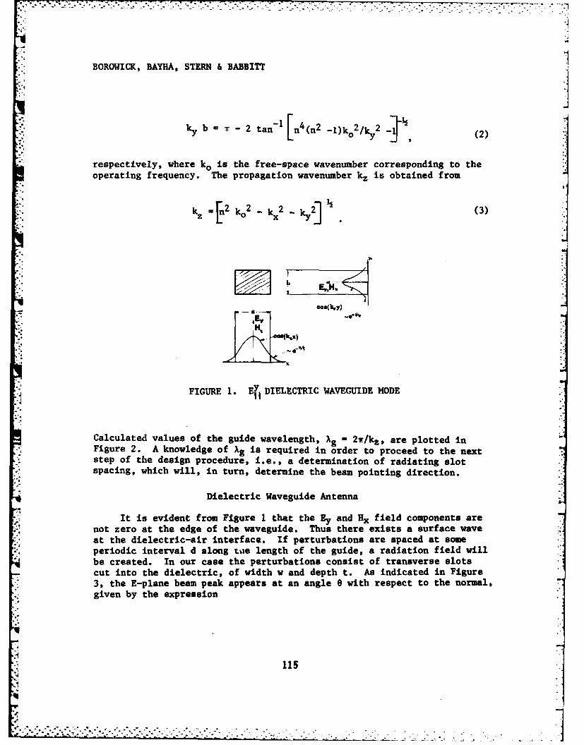
BOROWICK, BAYHA, STERN4 & BABBITT]
ky b = i = 2 tan - n4(n2 -1)ko 2/ky2 (2)
respectively, where ko is the free-space wavenumber corresponding to theoperating frequency. The propagation wavenumber kz is obtained from
kz n2 k0 2 kx2 ky2] (3)
EH• eos(k y)I0i±A "1
FIGURE 1. EfIDIELECTRIC WAVEGUIDE MODE
Calculated values of the guide wavelength, Xg - 2w/kz, are plotted inFigure 2. A knowledge of Ag is required in order to proceed to the nextstep of the design procedure, i.e., a determination of radiating slotspacing, which will, in turn, determine the beam pointing direction.
Dielectric Waveguide Antenna
It is evident from Figure 1 that the Ey and Hx field components arenot zero at the edge of the waveguide. Thus there exists a surface waveat the dielectric-air interface. If perturbations are spaced at someperiodic interval d along tie length of the guide, a radiation field willbe created. In our case the perturbations consist of transverse slotscut into the dielectric, of width w and depth t. As indicated in Figure3, the E-plane beam peak appears at an angle e with respect to the normal,given by the expression
115
E.
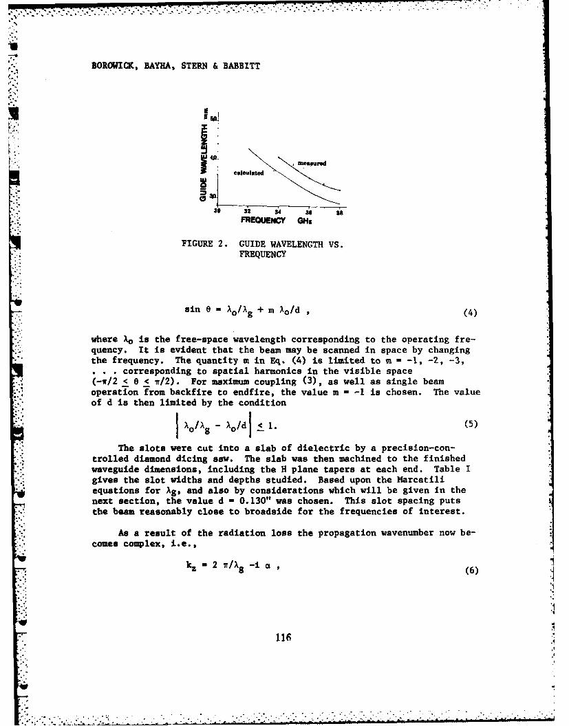
...
BOROWICK, BAYHA, STERN & BABBITT
4 measured
ealculated
30 32 34 36 38
-FREQUENCY GM
FIGURE 2. GUIDE WAVELENGTH VS.FREQUENCY
sin e XO/Ag + m Xo/d (4)
where Xo is the free-space wavelength corresponding to the operating fre-quency. It is evident that the beam may be scanned in space by changingthe frequency. The quantity m in Eq. (4) is limited to m = -1, -2, -3,
. corresponding to spatial harmonics in the visible space(-w/2 < e < ff/2). For maximum coupling (3), as well as single beamoperation from backfire to endfire, the value m = -1 is chosen. The value
.of d is then limited by the condition
S. - Xo/d < 1. (5)
The slots were cut into a slab of dielectric by a precision-con-trolled diamond dicing saw. The slab was then machined to the finishedwaveguide dimensions, including the H plane tapers at each end. Table Igives the slot widths and depths studied. Based upon the Marcatiliequations for Ag, and also by considerations which will be given in thenext section, the value d - 0.130" was chosen. This slot spacing putsthe beam reasonably close to broadside for the frequencies of interest.
As a result of the radiation loss the propagation wavenumber now be-comes complex, i.e.,
k 2 w/,g -i a, (6)S(
,',.. 11 .,
. .
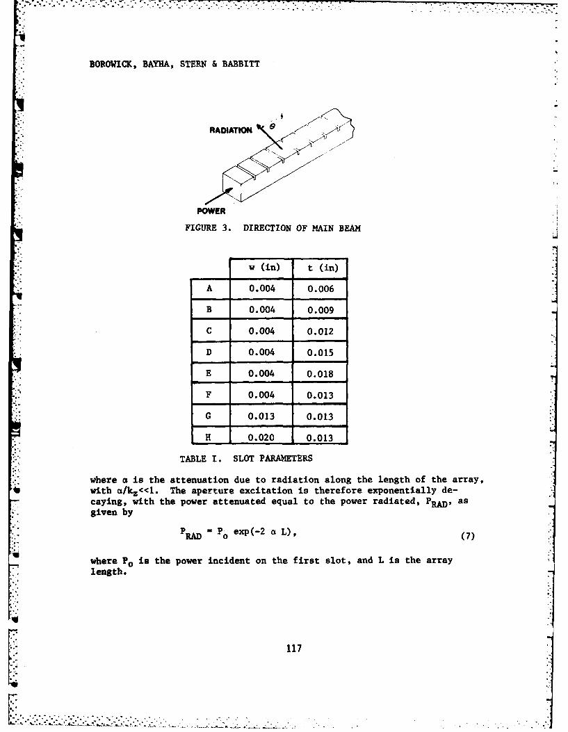
BOROWICK, BAYHA, STERN & BABBITT
RADIATION "
POWER
FIGURE 3. DIRECTION OF MAIN BEAM
w (in) t (in)
A 0.004 0.006
B 0.004 0.009
C 0.004 0.012
D 0.004 0.015
E 0.004 0.018
F 0.004 0.013
G 0.013 0.013
H 0.020 0.013
TABLE I. SLOT PARAMETERS
where a is the attenuation due to radiation along the length of the array,with a/kz<<l. The aperture excitation is therefore exponentially de-caying, with the power attenuated equal to the power radiated, PRAD' asgiven by
P Po exp(-2 a L),:"D 0 (7)
where Po is the power incident on the first slot, and L is the arraylength.
117
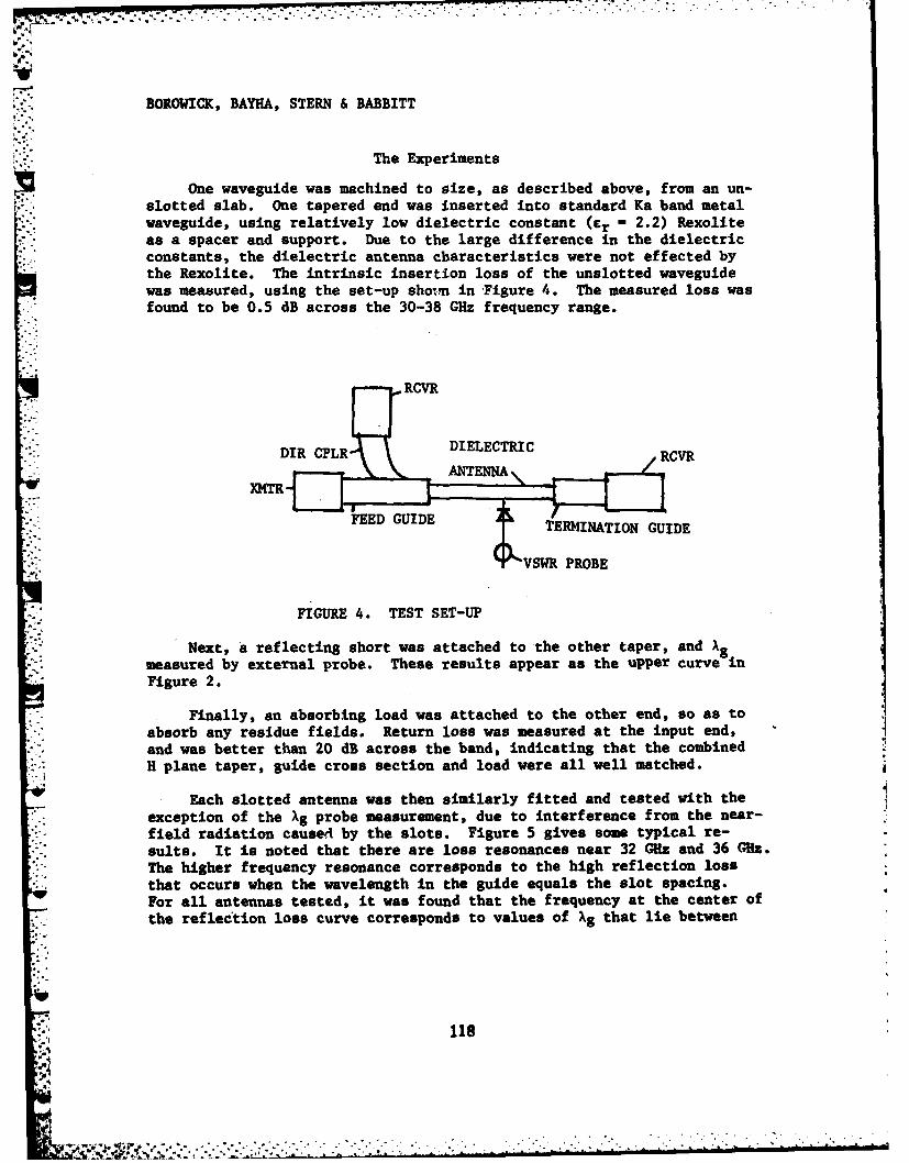
L ! ' " - ' " < . . .' " ' " " ' ' " " "' , " ' " " " ' ' " " . ..
..
.. BOROWICK, BAYHA, STERN & BABBITT
The Experiments
One waveguide was machined to size, as described above, from an un-slotted slab. One tapered end was inserted into standard Ka band metalwaveguide, using relatively low dielectric constant (Cr - 2.2) Rexoliteas a spacer and support. Due to the large difference in the dielectricconstants, the dielectric antenna characteristics were not effected bythe Rexolite. The intrinsic insertion loss of the unslotted waveguidewas measured, using the set-up shoim in Figure 4. The measured loss wasfound to be 0.5 dB across the 30-38 GHz frequency range.
;;'" DIELECTRIC. !DIR CPLR' RCVR
*-./ ANTENNA,
FEED GUIDE TERMINATION GUIDE
VSWR PROBE
FIGURE 4. TEST SET-UP
Next, a reflecting short was attached to the other taper, and ,gmeasured by external probe. These results appear as the upper curve inFigure 2.
Finally, an absorbing load was attached to the other end, so as toabsorb any residue fields. Return loss was measured at the input end,and was better than 20 dB across the band, indicating that the combinedH plane taper, guide cross section and load were all well matched.
Each slotted antenna was then similarly fitted and tested with theexception of the Ag probe measurement, due to interference from the near-field radiation caused by the slots. Figure 5 gives some typical re-sults. It is noted that there are loss resonances near 32 CHz and 36 GCZ.The higher frequency resonance corresponds to the high reflection lossthat occurs when the wavelength in the guide equals the slot spacing.For all antennas tested, it was found that the frequency at the center ofthe reflection loss curve corresponds to values of Xg that lie between
118
I= " . : ;; ' '. , .. " - i ; - i; , , : _ - - '. " , : . , . - ," " , " " '
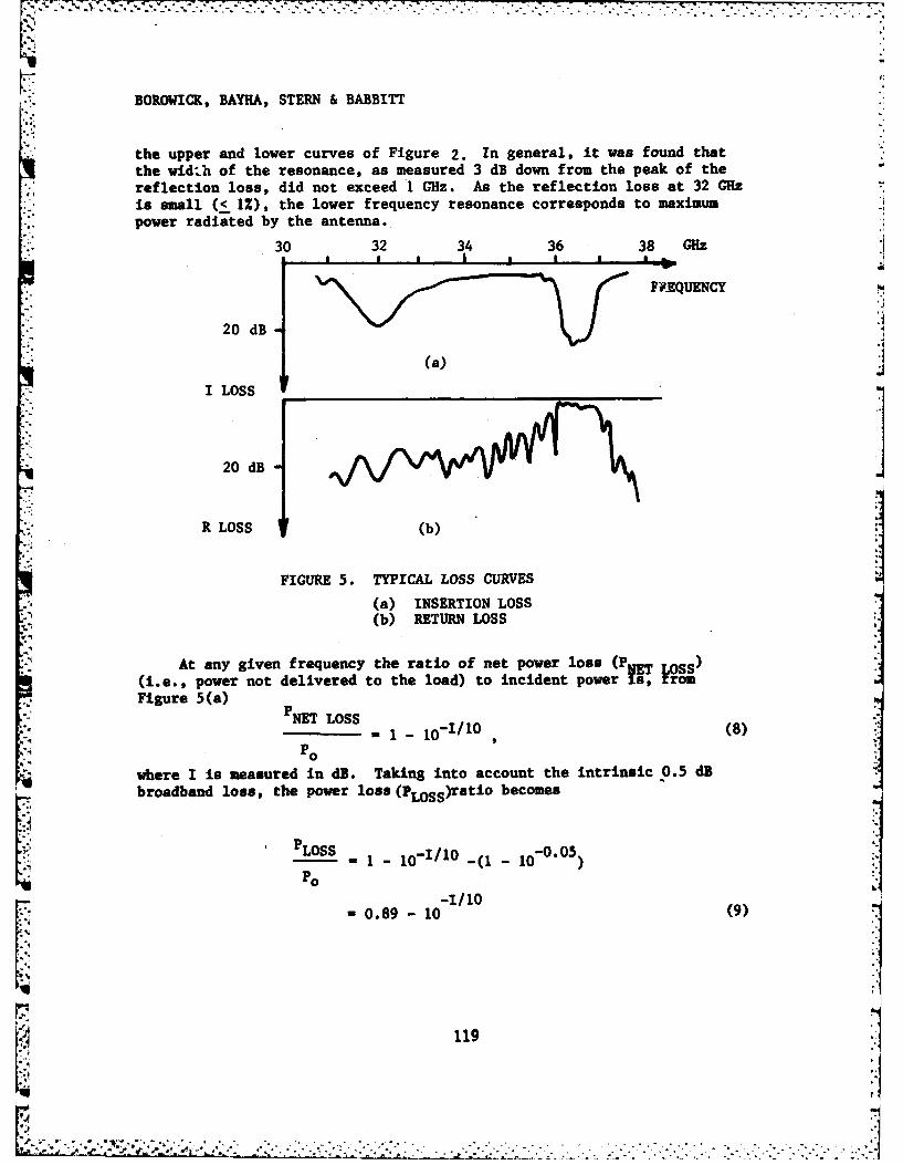
BOROWICK, BAYHA, STERN & BABBITT
the upper and lower curves of Figure 2. In general, it was found thatthe width of the resonance, as measured 3 dB down from the peak of thereflection loss, did not exceed 1 GHz. As the reflection loss at 32 GHz
is small (1 1%), the lower frequency resonance corresponds to maximumpower radiated by the antenna.
30 32 34 36 38 GHz
FREQUENCY
20 dB
(a)
I LOSS _
20 dB
R LOSS (b)
FIGURE 5. TYPICAL LOSS CURVES(a) INSERTION LOSS(b) RETURN LOSS
At any given frequency the ratio of net power loss (P ET JOSS )
(i.e., power not delivered to the load) to incident power is, romFigure 5(a)
" NET LOSS (I - 10- / 10 (8)
"1 P0where I is measured in dB. Taking into account the intrinsic 0.5 dB
broadband loss, the power loss (PLoSs)ratio becomes
LOSS = - 10 -1I/1O -(1 10 - 5);i Po
. 0.89 - 10 (9)
119: 2 'i .. . . . . .. . . . . .
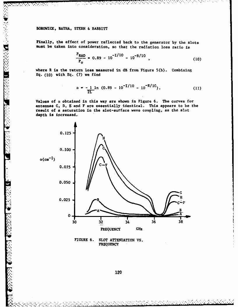
:.;.::.. . ,. -: .. . ... -. ....
BOROWICK, BAYHA, STERN & BABBITT
Finally, the effect of power reflected back to the generator by the slotsmust be taken into consideration, so that the radiation loss ratio is
PRAD -I/10 10- 0.89 - 10 10 (10)
P0
where R is the return loss measured in dB from Figure 5(b). CombiningEq. (10) with Eq. (7) we find
a --a 1 in (0.89 10- / 1 10 -R/10))
"-" 2L
Values of a obtained in this way are shown in Figure 6. The curves forantennas C, D, E and F are essentially identical. This appears to be theresult of a saturation in the slot-surface wave coupling, as the slotdepth is increased.
0.125-H
0.100 G
0 (cm-1)
0.075 -C-F
0.050
0.025
A B
0.
30 32 34 36 38
FREQUENCY GHz
FIGURE 6. SLOT ATTENUATION VS.FREQUENCY
120
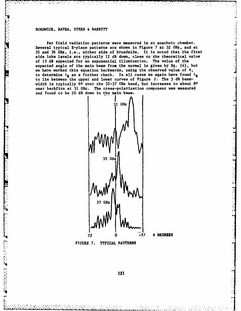
I.I
BOROWICK, BAYHA, STERN & BABBITT
q Far field radiation patterns were measured in an anechoic chamber. _Several typical E-plane patterns are shown in Figure 7 at 32 GHz, and at
35 and 36 GHz, i.e., either side of broadside. It is noted that the firstside lobe levels are typically 12 dB down, close to the theoretical valueof 13 dB expected for an exponential illumination. The value of theexpected angle of the main beam from the normal is given by Eq. (4), butwe have worked this equation backwards, using the observed value of 6,to determine Ag as a further check. In all cases we again have found gto lie between the upper and lower curves of Figure 2. The 3 dB beam-width is typically 60 over the 32-37 GHz band, but increases to about 80near backfire at 31 GHz. The cross-polarization component was measured.and found to be 20 dB down in the main beam.DI
32 GHz
35 Hz
I
37 GHz".
72 0 -72 e DEGREES
FIGURE 7. TYPICAL PATTERNS
121
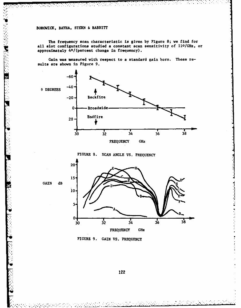
I ll I J II I -~~~~~~. .. .. .. . . . ... •...,.! . .:. . ..... ""' '.."..."". ." ..
BOROWICK, BAYHA, STERN & BABBITT
The frequency scan characteristic is given by Figure 8; we find forall slot configurations studied a constant scan sensitivity of 110/GHz, orapproximately 40/(percent change in frequency).
Gain was measured with respect to a standard gain horn. These re-sults are shown in Figure 9.
-60
e DEGREES -40
-20 Bacfire
0- - Broadside
20 Endf re
30 32 34 36 38
FREQUENCY GHz
FIGURE 8. SCAN ANGLE VS. FREQUENCY
20
15" C
GAIN dB H
10.1
5-
30 32 34 36 38
FREQUENCY GHz
FIGURE 9. GAIN VS. FREQUENCY
~122
BOROWICK, BAYHA, STERN & BABBITT
Conclusions
Investigations have continued into developing design criteria for adielectric waveguide line source antenna. The Marcatili analysis hasproven to be a reliable guide for the transmission line design. Thereis, however, no practical design information available permitting thesynthesis of a symmetrical amplitude taper along a grooved dielectricwaveguide antenna. This investigation presents a measurement procedurethat will permit a correlation between the radiating element physicalconfiguration and the radiation properties. Additional data for variousslot geometries will continue to be accumulated. A theoretical and em-
" perical relationship will then be made so as to further relate the slotgeometry to radiation characteristics. Our investigations have demon-strated that a non-metallic grooved dielectric waveguide can be made toradiate with a well-formed antenna pattern resulting from an exponentialamplitude taper. This effort will be extended to permit the design of alower sidelobe dielectric waveguide slot antenna.
Acknowledgement
The authors wish to thank Mr. William Johnson and Mr. Herbert Daleyfor their technical assistance, and Mrs. Phyllis Prorok for preparing themanuscript.
References
1. John Borowick, Richard A. Stern and Richard W. Babbitt, "A SmallElectronic Scan Angle Antenna for Millimeter Waves", ERADCOM ReportDELCS-TR-81-2, September 1981.
2. E.A.J. Marcatili, "Dielectric Rectangular'Waveguide and DirectionalCoupler for Integrated Optics", Bell System Technical Journal,Volume 48, No. 7, pp 2071-2102, September 1969.
3. Johannes Jacobsen, "Analytical, Numerical, and Experimental Inves-tigation of Guided Waves on a Periodically Strip-Loaded DielectricSlab", IEEE Transactions on Antennas and Propagation, Volume AP-18,No. 3, pp 379-388, May 1970.
123
V ... . .
BOWDEN
MICOM PROGRAM IN LIGHT CONTROL BY LIGHT (U)
CHARLES M. BOWDEN, DR.IESEARCH DIRECTORATE, US ARMY MISSILE LABORATORY
US ARMY MISSILE COMMNDREDSTONE ARSENAL, ALABAMA 35898
1. INTRODUCTION
Superfluorescence (1) is the phenomenon whereby a collection of atomsor molecules is prepared initially in a state of complete inversion, andthen allowed to undergo relaxation by collective, spontaneous decay. Thisproduces pulses of anomalous intensity (proportional to the square of thedensity of active atoms) and of anomalous, temporal duration (inverselyproportional to the density). Since Dicke's initial work (2), there hasbeen a preponderance of theoretical and experimental work dealing withthis process (3).
With the exception of the more recent work of Bowden and Sung (4),all theoretical treatments have dealt exclusively with the relaxation pro-cess from a prepared state of complete inversion in a two-level manifoldof atomic energy levels, and thus do not consider the dynamical effects ofthe pumping process. Yet, all reported experimental work (3,5-10) hasutilized optical pumping on a minimum manifold of three atomic or molecu-lar energy levels by laser pulse injection into the nonlinear medium,which subsequently fluorescesces.
It was pointed out by Bowden and Sung (4) that for a system otherwisesatisfying the conditions for superfluorescent emission, unless the char-acteristic superradiance time (1), TR, is much greater than the pump pulsetemporal duration, Tp, i.e., TR > > Tp, the process of coherent opticalpumping on a three-level system can have dramatic effects on the SF. Thisis a condition which has not been realized over the full range of report-ed data.
In this paper, we present calculational results and analysis for theeffects of coherent pump dynamics, propagation, transverse and diffractioneffects on SF emission from an optically-pumped three-level system. Thefull, nonlinear, co-propagational aspects of the injected pump pulse, to-gether with the SF which evolves are explicitly treated in the calculation.
125
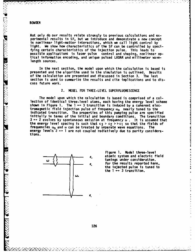
BOWDEN
Not only do our results relate strongly to previous calculations and ex-perimental results in SF, but we introduce and demonstrate a new conceptin nonlinear light-matter interactions, which we call light control bylight. We show how characteristics of the SF can be controlled by speci-fying certain characteristics of the injection pulse. This leads topossible applications in laser pulse control and shaping, nonlinear op-tical information encoding, and unique pulsed LADAR and millimeter wave-length sources.
In the next section, the model upon which the calculation is based ispresented and the algorithm used in the simulation is outlined. Resultsof the calculation are presented and discussed in Section 3. The lastsection is used to summarize the results and cite implications and to dis-cuss future work.
2. MODEL FOR THREE-LEVEL SUPERFLUORESCENCE
The model upon which the calculation is based is comprised of a col-lection of identical three-level atoms, each having the energy level schemeshown in Figure 1. The 1 +-* 3 transition is induced by a coherent elec-tromagnetic field injection pulse of frequency wo nearly tuned to theindicated transition. The properties of this pumping pulse are specifiedinitially in terms of the initial and boundary conditions. The transition3 4-+ 2 evolves by spontaneous emission at frequency w . It is assumed thatthe energy level spacing is such that e3 > £2 >>el so that the fields offrequencies to and w can be treated by separate wave equations. Theenergy levels 2 - 1 are not coupled radiatively due to parity considera-tions.
Figure 1. Model three-levele, atomic system and electric field
tunings under consideration.For the results reported here,the injected pulse is tuned tothe 1 - 3 transition.
12
- % -..
-" - 126.. . . . . .
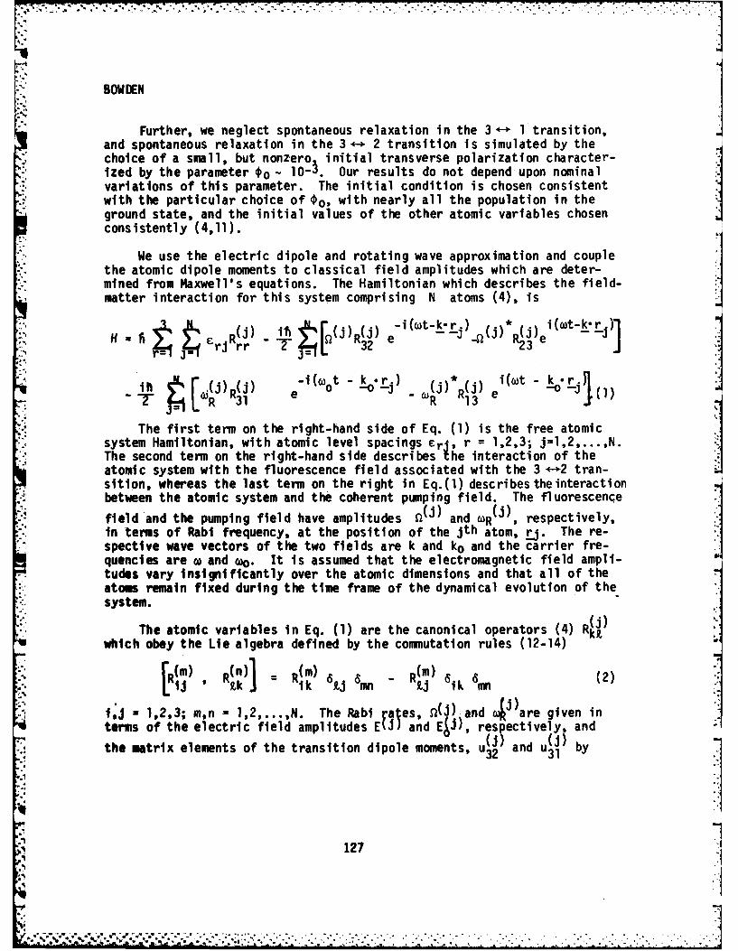
BOWDEN
Further, we neglect spontaneous relaxation in the 3 - 1 transition,and spontaneous relaxation in the 3+- 2 transition is simulated by thechoice of a small, but nonzero initial transverse polarization character-ized by the parameter €o - 10-5. Our results do not depend upon nominalvariations of this parameter. The initial condition is chosen consistentwith the particular choice of €o, with nearly all the population in theground state, and the initial values of the other atomic variables chosenconsistently (4,11).
We use the electric dipole and rotating wave approximation and couplethe atomic dipole moments to classical field amplitudes which are deter-mined from Maxwell's equations. The Hamiltonian which describes the field-matter interaction for this system comprising N atoms (4), is
Hf = 6 q, R(j) - .i! 'FfJR(j)32 -i(it-kr )(J* ( i(t-kr.)]~ 32 e 0 e Jr' rJ rr-ee
it h '(i)(i) -i(°t - k-°r-.) -e 0 (j)*R(j) e -° l
- 7R 3~0 1 e- - R 13-k
The first term on the right-hand side of Eq. (1) is the free atomicsystem Hamiltonian, with atomic level spacings cri, r = 1,2,3; J=I,2,...,N.The second term on the right-hand side describes the interaction of theatomic system with the fluorescence field associated with the 3 +-*2 tran-sition, whereas the last term on the right in Eq.(l) describes theinteractionbetween the atomic system and the coherent pumping field. The fluorescence
field and the pumping field have amplitudes f(J) and wR(j ), respectively,in terms of Rabi frequency, at the position of the jth atom, rj. The re-
spective wave vectors of the two fields are k and ko and the carrier fre-quencies are w and o. It is assumed that the electromagnetic field ampli-tudes vary insignificantly over the atomic dimensions and that all of theatoms remain fixed during the time frame of the dynamical evolution of thesystem.
The atomic variables in Eq. (1) are the canonical operators (4) R )
which obey the Lie algebra defined by the commutation rules (12-14)
[R(m) R(n)R(m) (2),i) 'R = Rik j 6mn - Rj 6ik 6an (2)
i;j - 1,2,3; m,n = 1,2,...,N. The Rabi rales, D(.) and 4::are given interms of the electric field amplitudes EU) and Epi), respectively, and
the matrix elements of the transition dipole moments, u32 and u31 bY
127
(I u j
I, I'= ' ., ' + # . , _ ,. .. .. . ._ ...

-V
C BOWIDEN
E(J)u(J) E(,i)u(J)
(J) 32 C00) 0 31 (3a,b)
-.,. where we have considered only one linear polarization for the two fieldsand propagation in the positive z direction.
It is convenient to introduce a new set of variables in terms of theold ones. We let
W R - Rtt , k > ; Rk =1 (U + Vk) , k > , (4ab)
where Uk9,V , and Wk9 are real variables, and Uk= Utk, Vkt = k
= X + iY ; (RXo+iYo , (4c,d)
where X, Y, X0 and Yo are real variables which are functions of both spaceand time.
The equations of motion for the atomic variables are calculatedaccording to the commutation relation
~)=rkt I kt] 5If the transformation, Eqs. (4) is applied to the hierarchy of Eqs. (5),the resulting equations of motion for the real variables W SUkVkilare
=31 2 {XU32 " YV32} + {XoU 31 o "'311 [W3 1 " wl)j . (6a,
.W1 2 = XU32 YV32) + {oU31I Yo3I "ll 3 X Wo3l *132" -W ) (6b)
U3 Y V Y W~e) (6b)::.;U32 6 "V32 "W X32 + [. oU12 -YoV12 - Y1U32 ,(6c0
V3 2 =U 32 + YW32 " XoV2 1 + YoU - Y (6d)
U31 = AV3 1 + T' 1XU21 + " XW31 31 , (6e)
... AU31 (6f)V31 U31 + 7"XV21 Y + YW 31 31
12R
* ,..-- . . ..
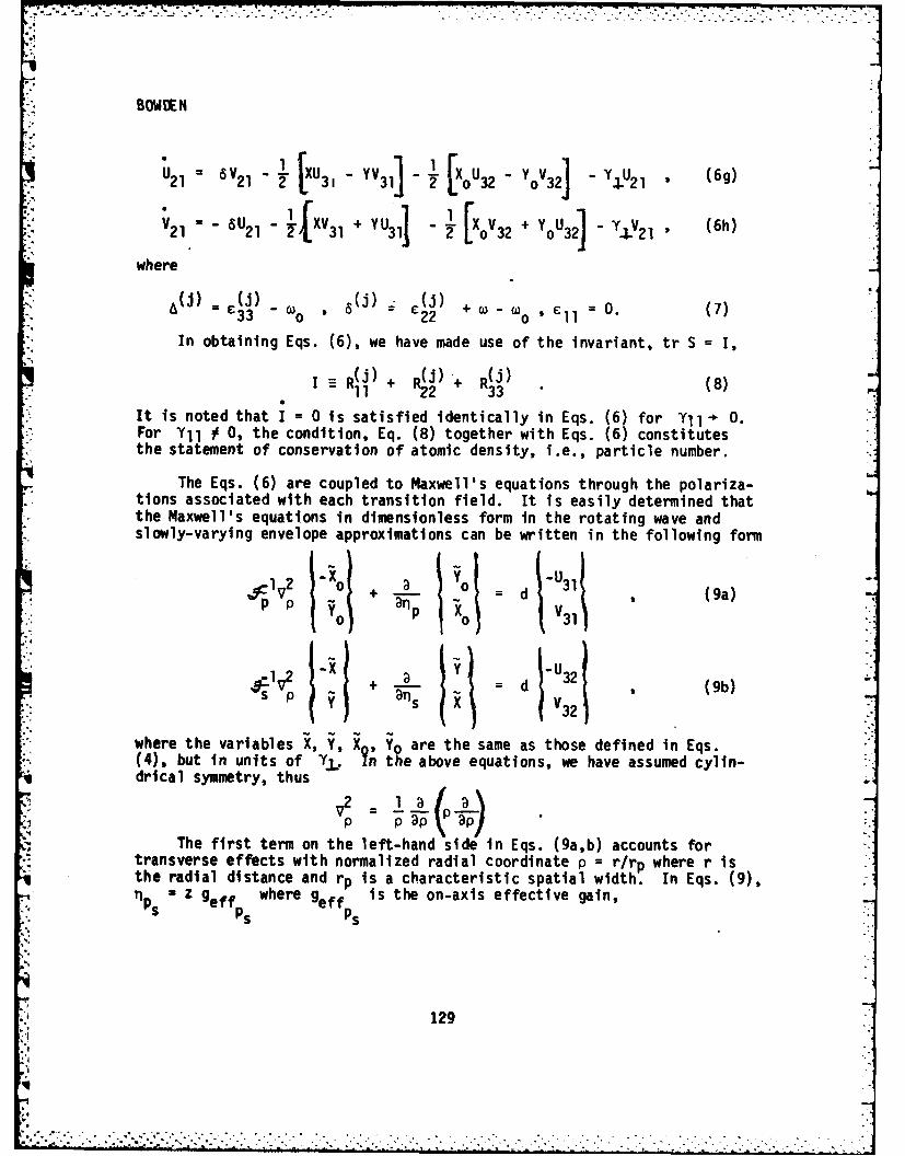
BOWDEN
U2 6V21 - X [x3 1 v31] 21~ [xoU 32 -o32 .2 ('g)
2 -. 21 ._ u - YU3 - - [XoV32 o 32] - - 21
where
a0 ) C 0) - o ( j ) _: C() + C3- E 0. (7)
(3320' 011 2 (7
In obtaining Eqs. (6), we have made use of the invariant, tr S = I,
I = RO ) + ) + R ) (8)
11 R 33 "* It is noted that I = 0 is satisfied identically in Eqs. (6) for YII-- 0.
For YII 0 0, the condition, Eq. (8) together with Eqs. (6) constitutesthe statement of conservation of atomic density, i.e., particle number.
The Eqs. (6) are coupled to Maxwell's equations through the polariza-tions associated with each transition field. It is easily determined thatthe Maxwell's equations in dimensionless form in the rotating wave andslowly-varying envelope approximations can be written in the following form
, 1v2 "X 0 + = d 31 (9a)" P P Yo np V3
1+ _X + = d _U , (9b)Bs V ( 32 :
where the variables X, Y, X ,o are the same as those defined in Eqs.(4), but in units of YJ.. ?n the above equations, we have assumed cylin-drical symmetry, thus
V2 1
The first term on the left-hand side in Eqs. (9a,b) accounts fortransverse effects with normalized radial coordinate p = r/rp where r isthe radial distance and rp is a characteristic spatial width. In Eqs. (9),ps z geff where g is the on-axis effective gain,
129
4 ° , - o . ° • q .. -. . , • . . . * ° ° ., ° . . . • -. . . , . . . °-
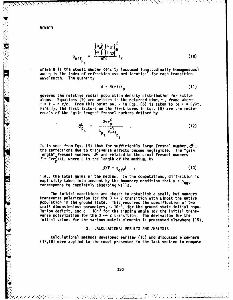
BOWDEN
PS = [ L T (10)"eff - nc 2Ps
where N is the atomic number density (assumed longitudinally homogeneous)and nj is the index of refraction assumed identical for each transitionwavelength. The quantity
d = N(r)/N ° (11)
governs the relative radial population density distribution for activeatoms. Equations (9) are written in the retarded time, t, frame whereT = t - n z/c. From this point on, - in Eqs. (6) is taken to be =/T.Finally, the first factors on the first terms in Eqs. (9) are the recip-rocals of the "gain length" Fresnel numbers defined by
2wr2-- g--- .(12)
ps effs p5
It is seen from Eqs. (9) that for sufficiently large Fresnel number, 5-,the corrections due to transverse effects become negligible. The "gainlength" Fresnel numbers 'f are related to the usual Fresnel numbersF = 2nr 2/XL, where L is the length of the medium, by
p/F = gffL (13)
i.e., the total gains of the medium. In the computations, diffraction isexplicitly taken into account by the boundary condition that p = pmaxcorresponds to completely absorbing walls.
The initial conditions are chosen to establish a small, but nonzerotransverse polarization for the 3 +-* 2 transition with almost the entirepopulation in the ground state. This requires the specification of twosmall dimensionless parameters, _lO -3 , for the ground state initial popu-lation deficit, and 6 10-3 for the tipping angle for the initial trans-verse polarization for the 3 *-' 2 transition. The derivation for theinitial values for the various matrix elements is presented elsewhere (15).
3. CALCULATIONAL RESULTS AND ANALYSIS
Calculatlonal methods developed earlier (16) and discussed elsewhere(17,18) were applied to the model presented in the last section to compute
130
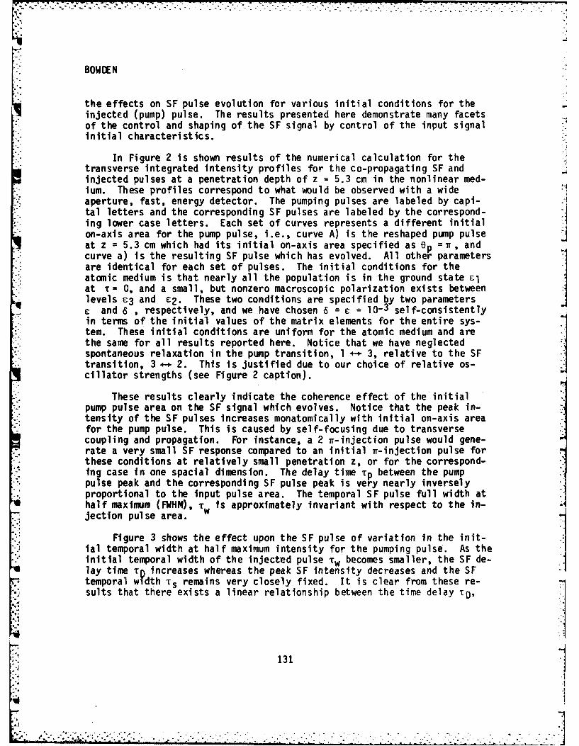
BOW DEN
the effects on SF pulse evolution for various initial conditions for theinjected (pump) pulse. The results presented here demonstrate many facetsof the control and shaping of the SF signal by control of the input signal
* initial characteristics.
In Figure 2 is shown results of the numerical calculation for thetransverse integrated intensity profiles for the co-propagating SF andinjected pulses at a penetration depth of z = 5.3 cm in the nonlinear med-ium. These profiles correspond to what would be observed with a wideaperture, fast, energy detector. The pumping pulses are labeled by capi-tal letters and the corresponding SF pulses are labeled by the correspond-ing lower case letters. Each set of curves represents a different initialon-axis area for the pump pulse, i.e., curve A) is the reshaped pump pulseat z = 5.3 cm which had its initial on-axis area specified as ep =7r, andcurve a) is the resulting SF pulse which has evolved. All other parameters
: are identical for each set of pulses. The initial conditions for theatomic medium is that nearly all the population is in the ground state Elat T= 0, and a small, but nonzero macroscopic polarization exists betweenlevels E3 and E2. These two conditions are specified by two parametersc and 6 , respectively, and we have chosen 6 = e l0-3 self-consistentlyin terms of the initial values of the matrix elements for the entire sys-tem. These initial conditions are uniform for the atomic medium and arethe same for all results reported here. Notice that we have neglectedspontaneous relaxation in the pump transition, 1 *-- 3, relative to the SFtransition, 3 +-, 2. This is justified due to our choice of relative os-cillator strengths (see Figure 2 caption).
These results clearly indicate the coherence effect of the initialpump pulse area on the SF signal which evolves. Notice that the peak in-tensity of the SF pulses increases monatomically with initial on-axis areafor the pump pulse. This is caused by self-focusing due to transversecoupling and propagation. For instance, a 2 ir-injection pulse would gene-rate a very small SF response compared to an initial i-injection pulse forthese conditions at relatively small penetration z, or for the correspond-ing case in one spacial dimension. The delay time Tp between the pumppulse peak and the corresponding SF pulse peak is very nearly inverselyproportional to the input pulse area. The temporal SF pulse full width at
* half maximum (FWHM), Tw is approximately Invariant with respect to the in-jection pulse area. w
Figure 3 shows the effect upon the SF pulse of variation in the init-ial temporal width at half maximum intensity for the pumping pulse. As theinitial temporal width of the injected pulse Tw becomes smaller, the SF de-
V lay time TD increases whereas the peak SF intensity decreases and the SFtemporal width T s remains very closely fixed. It is clear from these re-sults that there exists a linear relationship between the time delay TD,
131
---
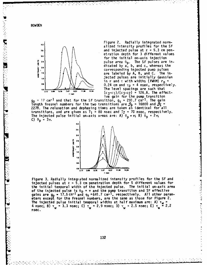
•.7
BOWDEN
4.0 Figure 2. Radially integrated norm-alized intensity profiles for the SF
3.5 and injected pulse at z = 5.3 cm pen-&0 /etration depth for 3 different values
- for the initial on-axis injection2.5 pulse area Op The SF pulses are in-
2.0 dicated by a, b, and c, whereas thecorresponding injected pump pulses
",.5 are labeled by A, B, and C. The in-
in r and T with widths (FWHM) r o =0.5 0.24 cm and Tp.= 4 nsec, respectively.0.0 The level spacings are such that, 2.17 3.90 5.70 7.47 9.37 IIM3 13.U4
2130. (E3 -61)/( 3-e2) = 126.6. The effect-ive gain for the pump transition
gp = 17 cm-1 and that for the SF transition, gs = 291.7 cm-1 . The gainlength Fresnel numbers for the two transitions are5_p = 16800 and 4 =2278. The relaxation and dephasing times are taken as identical for alltransitions, and are given as T1 = 80 nsec and T2 = 70 nsec, respectively.The injected pulse initial on-axis areas are: A) Op: T; B) O =C) 0p =3.
4.0
3.0
E 2.5Z
.%'I<1.0
IS o1.0 A
0.5
2.17 3."0 5.70 7.47 9.37 11.5 13.34
Figure 3. Radially integrated normalized intensity profiles for the SF andinjected pulses at z = 5.3 cm penetration depth for 5 different values forthe initial temporal width of the injected pulse. The initial on-axis areaof the injected pulse is Op = ir and the pump transition and SF effectivegains are g = 17.5 cm-I and qs =641.7 cm- 1 , respectively. All other param-eters except for the Fresnel numbers, are the same as those for Figure 2.The injected pulse initial temporal widths at half maximum are: A) Tw =4 nsec; B) Tw =3.3 nsec; C) Tw = 2.9 nsec; D) T = 2.5 nsec; E) T =2.2
nsec. w w w
132
:::. .
-.. 4BOWDEN"
between the peak SF intensity and the corresponding pump pulse intensity,and the initial temporal width Tw of the pump pulse. This is in qualita-tive agreement with the analytical prediction made in reference 4b, Eq.5.1, based upon mean field theory. These results emphasize the import-ance of the initiating pulse characteristics in SF pulse evolution, andthe effect of SF pulse narrowing with approximate pulse shape invarianceby increasing the initial temporal width of the injected pulse. It isemphasized that all other parameters, including the initial value for theinjected pulse on-axis area, are identical among these sets of curves.
The initial radial width, rp, of the injected pulse was varied andthe effect upon the SF pulse evolution is shown in Figure 4. There isclearly indicated an optimum value for rp for which the SF peak inten-sity is a maximum and the SF temporal width t s is a minimum. If the re-lation, Eq. (13) is used in conjunction with the values of the parametersgiven in Figure 4 and its caption, it is seen that optimization occursfor a value for the conventional Fresnel number Fs for the SF transition,Fs 1. Thus, from Eq. (13) and Fs = 1, we have
O fos = gs z (14)
for the gain-length Fresnel number. Since Fs -l/z the implication is thatEq. (14) gives the penetration depth, zmax, at which the SF peak intensity
;'* reaches a maximum in terms of the ratio s/gs. Since this takes bothtransverse and diffraction explicitly into account as well as propagation,this is indeed a profound statement.
Further insight into the implication of Eq. (14) can be obtained byconsidering a one-spacial dimension analogy. If the linear field loss istaken to be entirely due to diffraction, then the one-dimensional linearloss c corresponding to the two-dimensional case specified by ., isgiven y
K = "(15).,,p
Then, from Eq. (12)= gs/s (16)
is the effective gain, gs, to loss, KS, ratio. From the condition, Eq.(14).
zmax s (;l) (17)
i.e.., Zmax is the penetration depth at which the SF peak intensity is amaximum, and corresponds to one effective diffraction length, as
133
....................................... ,
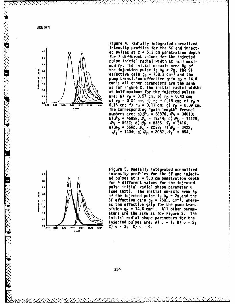
BOW DEN
Figure 4. Radially integrated normalizedintensity profiles for the SF and inject-
4.0 ed pulses at z = 5.3 cm penetration depth35 for 7 different values for the injected
pulse initial radial width at half maxi-&0 mum rp. The initial on-axis area 6p ofe ,,the injection pulse is ep = 2w; the SF
Ieffective gain gs = 758.3 cm-1 and thepu. transition effective gain gp= 14.6cm-; all other parameters are t sameas for Figure 2. The initial radial widthsat half maximum for the injected pulses
.are: a) r = 0.57 cm; b) rp = 0.43 cm;) rp = 0.24 cm; d) rp = 0.18 cm; e) rp
.1 &, 0 &70A7, . I,,JS 137. 0.15 cm; f) rp 0.11 cm; g) rp - 0.09 cm.Town ' The corresponding "gain length' Fresnel%:,• ":'numbers are: a).-p = 82876, Os - 34010;
"b),p = 46898,-#s = 19244; c). = 14428,J. = 5922; d) o*p = 8326, 3416;e) =5602, .s'= 2298; f) o = 3422,
:.-:'cf-s' 1404; g) -p =2082. -s = 854.
Figure 5. Radially integrated normalized4.0 intensity profiles for the SF and inject-
31 ed pulses at z = 5.3 cm penetration depth3b for 4 different values for the injected&0 pulse initial radial shape parameter v2.5 (see text). The initial on-axis area ep
,,.-S
g.,.of the injected pulse is p t 2 S and the20 SF effective gain g = 758.3 t i where-
[15as the effective gain for the pump tran-a sition g a 14.6 cm- 1. All other param-
1.0 eters A the same as for Figure 2. The0.5 initial radial shape parameters for the
injected pulses are: A) v 1; B) v 2;002.17 3.S0 5. 7.47 6.37~ IA C3A v=3; D) v4.
134
BOWD EN
defined by Eq. (15). Carrying the one-dimensional analogy one step fur-ther, Eq. (16) used in Eq. (13) gives
F = (KZ) (18)
From Eqs. (16) and (18) we have exhibited the significance of the Fresnelnumbers -% and F in terms of diffraction loss, i.e., -4 can be thought ofas gain to loss ratio, Eq. (16), whereas F can correspondingly be thoughtof as the reciprocal of the strength of the diffraction loss, Eq. (18).
The effect on SF pulse evolution of variation of the initial radialshape of the initiating pulse is shown in Figure 5. The shape parameterv is defined in terms of the ;nitial condition for the pump transitionfield amplitude, wR(r) ,
.- R r) = a)R(O) exp I- (r/rp ) . (19)
Thus, for v = 2, the initial amplitude of the injected pulse is radiallyGaussian, whereas for v - 4, it is radially super-Gaussian. We see fromthe results presented in Figure 5 that as the initial radial shape of theinjected pulse becomes broader, i.e., larger values for v , the peak in-tensity of the SF pulse generated becomes larger, and the width Ts dimin-ishes. It is emphasized that all other parameters, including the initialvalues for the radial and temporal widths are invariant among these setsof curves.
s,.,The response of SF pulse evolution to changes in the initial temporalshpe of the injection pulse is shown in Figure 6 which compares the effectof a Gaussian initial temporal shape for the pump pulse, identified by thetemporal shape parameter, a - 2, with that of a super-Gaussian identifiedby a = 4. As for the radial distribution discussed previously, the tem-poral shape parameter a is defined in terms of the initial condition forthe pump transition field amplitude (R( ) ,
(T - R(O) exp [4 . (20)
Again, it is seen that the broader initial pump pulse causes an increasein the peak SF intensity and a reduction in the delay time TD and SF pulsewidth -r D
Finally, Figure 7 shows the effect of variation of the density p ofactive atoms. The effective gains, gs and gp, are changed proportionally,corresponding to a density variation p . The ratio of the SF intensitiesis Ic/Ib - 1.76 and Ib/Ia 2.06; these ratios are larger than the
4 136
i . : 4%.. ,_ ..- .., .. .., . ,, - ,.- - ... .- - - -,- - - . . . . . .. .4. -. .. -.,. . . 4-.. .-, .. - -, - - - - -. .. . .
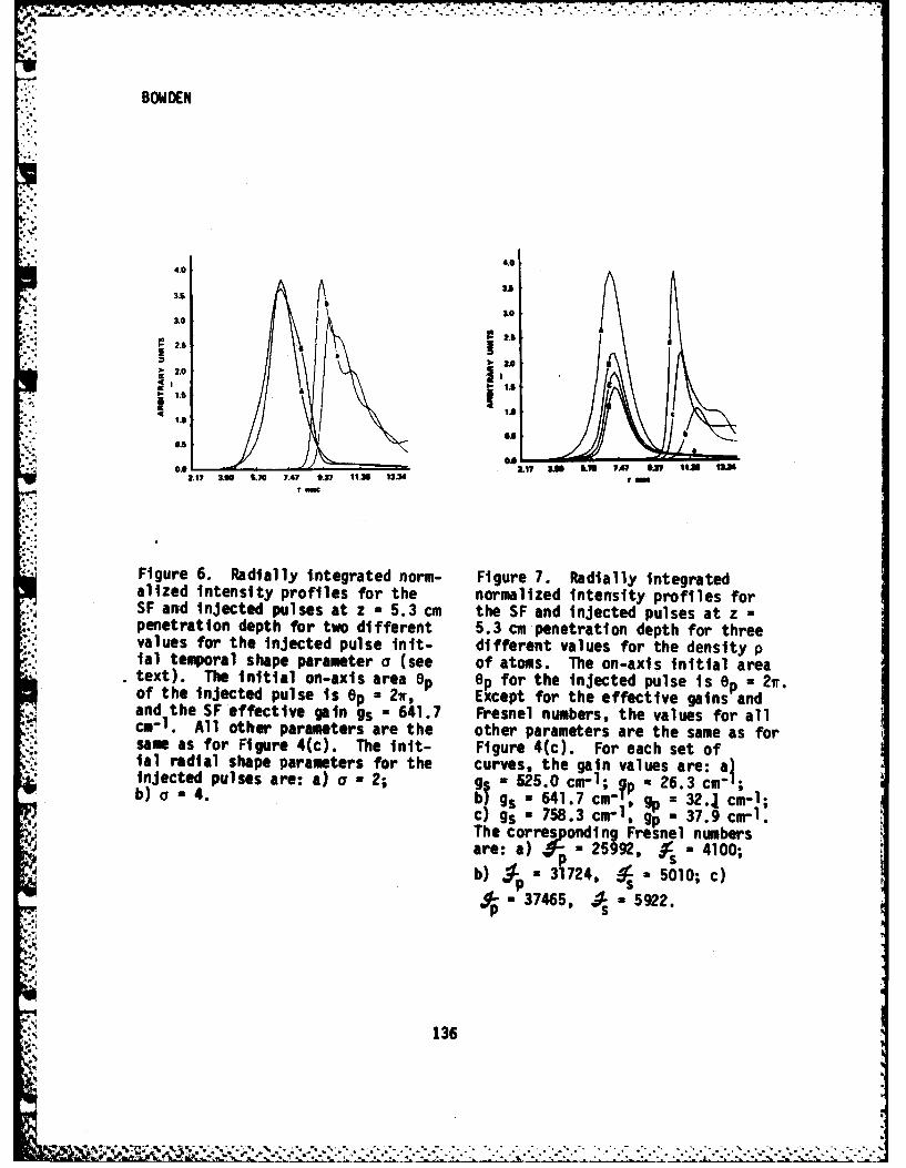
N7; BOWDEN
,.0
j' 4.04.0
3A
&0 &
2.8 2.6
20
'IIs. LA 1.
Isb
O.S
0.0 2.17 2.8 Lie ?A7 &V 1I1 ON2.17 3A.1 U70 7.47 9.7 11.1 13.34 1 own
r low
Figure 6. Radially integrated norm- Figure 7. Radially integratedalized intensity profiles for the normalized intensity profiles forSF and injected pulses at z - 5.3 cm the SF and injected pulses at z =
penetration depth for two different 5.3 cm penetration depth for threevalues for the injected pulse init- different values for the density pial temporal shape parameter a (see of atoms. The on-axis initial areatext). The initial on-axis area ep ep for the injected pulse is ep = 2w.of the injected pulse is ep 2w, Except for the effective gains andand the SF effective gain gs " 641.7 Fresnel numbers, the values for allcm- 1 . All other parameters are the other parameters are the same as forsame as for Figure 4(c). The mnit- Figure 4(c). For each set of.al radial shape parameters for the curves, the gain values are: abnjected pulses are: a) a - 2; g5 - 525.0 cm-1; Ip * 26.3 cm-1;b) a - 4. b) gs - 641.7 cm-1, gp = 32.a cm- 1 ;
c) gs" 758.3 cm-1, gp- 37.9 cull.The corresponding Fresnel numbersare: a) - 25992, As = 4100;
b) . - 31724, .a5010; c)p s
JZ - 37465, AL 5922.
136
BOWDEN
2 2corresponding density ratios squared (1), (PC/Pb) =1.40 and (Pb/Pa)21.49. This difference may be due to self-focusing, especially since thevalues of the effective gains used in this case are quite high. However,the ratio of the temporal widths, -w, (FWHM), is within 15% of the corres-ponding inverse ratios of the densities; the same is true for the delaytime, TD, Of the SF intensity peak with respect to the pump intensity peak.These results compare qualitatively reasonably well with the mean fieldpredictions for SF in two-level systems initially prepared in a state ofcomplete Inversion (1).
4. CONCLVIONS
The results presented here clearly demonstrate the coherence and de-terministic effects on SF pulse evolution of injection pump pulse initialcharacteristics and conditions. It is suggested that effects of the typediscussed here may have in fact been operative in SF experiments and theirresults which were published earlier (5-10).
Furthermore, and perhaps of greater importance, we have demonstratedthe control and shaping of the SF pulse which evolves, by specification ofparticular initial characteristics and conditions for the pumping pulsewhich is injected into the nonlinear medium to initiate SF emission. Thesemanifestations and others of the same class, we call the control of lightby light via a nonlinear medium. This phenomenon constitutes a method fornonlinear information encoding, or information transfer, from the injectionpulse characteristics to corresponding SF pulse characteristics whichevolve due to propagation and interaction in the nonlinear medium.
Work is now in progress to incorporate the effects of quantum statis-tics of the SF spontaneous relaxation process (19). We are in the processof further determination and analysis of the nonlinear interaction betweentwo co-propagating pulses resonantly, as well as nonresonantly, interact-ing by a nonlinear medium (19).
ACKNOWLEDGEMENT
Continued and valued collaboration with F. P. attar, Y. Claude andM. Cormier is gratefully acknowledged.
REFEENCES
1. R. Bonifacio and L. A. Lugiato, Phys. Rev. All, 1507 (1975); A12,587 (1975).
2. R. H. Dicke, Phys. Rev. 93, 99 (1954).
137
7:. . . . . . - - - , ~
BOW DEN
3. See papers and references in Cooperative Effects in Matter andRadiation, edited by C. M. Bowden, 0. W. Howgate and H. R. Robi, Plenum,New York, (1977). "Swept-gain Superradiance in C02-pumped CI13F", J. J.Ehrlich, C. M. Bowden, S. H. Lehnigk, A. T. Rosenberger and T. A. DeTemple,in Coherence and Quantum Optics IV, edited by 1. Mandel and E. Wolf,Plenum, New York, p. 9Z3 (1978). "MIRADCOM Program in Swept-gain Super-Radiance", D. W. Howgate, C. M. Bowden and 3. J. Ehrlich, US Army ScienceConference Proceedings, June (1978), First Prize.
4. C. N. Bowden and C. C. Sung, Phys. Rev. A18, 1558 (1978); Phys.Rev. A20, 2033 (1979).
5. N. Skirbanowitz, 3. P. Herman, J. C. MacGillivray and M. S. Feld,Phys. Rev. Lett. 30 309 (1973).
6. H. N. Gibbs, Q. H. F. Vrehen and H. M. J. Hickspoors, Phys. Rev.Lett. 39, 547 (1977).
7. Q. H. F. Vrehen, in Cooperative Effects in Matter and Radiation,edited by C. N. Bowden, D. W . Howgate and H. R. Robl, Plenum, New YORk,p. 79 (1977).
8. M. Gross, C. Fabre, P. Pillet and S. Haroche, Phys. Rev. Lett.36, 1035 (1976).
9. A. Flusberg, F. ?'bssberg and S. R. Harwtmann, in Coperati~veEffects inMatter and Radiation, edited by C. N. Bowden, D. W. Hoite
adH. R. Robl, Plernum, New York, p. 379 (1977).
10. A. T. Rosenberger and T. A. DeTemple, Phys. Rev. A24, 868 (1981).
11. F. T. Hioe and J. H. Eberly, Phys. Rev. Lett. 47, 838 (1981).
12. R. Gilmore, Lie Groups. Lie Algebras, and Some of Their Applica-tions, Wiley, New York, Chapter 5, Section 2, (1974).
13. R. Gilmore, C. N. Bowden and 1. N. Narducci, Phys. Rev. A12,1019 (1975).
14. R. Gilmore, C. N. Bowden and L. N. Narducci, "c-Number Represen-tation for Multilevel System and the Quantum-Classical Correspondence",Iin quantum Statistics and the Many-Body Problem edited by S. B. Trickey,W. R. Kirk and J. W. Dufty, Plenum, New York, (i975).
138
.........

15. F. P. Mattar and C. M. Bowden, "Coherent Pump Dynamics and
Pulse Evolution in Three-level Superfluorescence and Control of Light byLight", in Topics in Current Physics: Multiple Photon Dissociation ofPolyatomic Molecules, eied by C. D. Cantrell, Springer-Verlag, Nei York,to appear, (1982).
16. F. P. Mattar and M. C. Newstein, in Cooperative Effects inMatter and Radiation, edited by C. M. Bowden, D. W. Howgate and H. R.Robl, Plenum, New York, p. 139 (1977).
17. F. P. Mattar, in 2ptia istiifty, edited by C. M. Bowden,N. Ciftan and H. R. Robi, Plnm Ne ork, p. 503 (1981); in PrceigTenth Simulation and Modeling Conference, Pitbrh 978 edit bW. Vogt and N. Mickle, Publ. Inst. Soc. Am., Pittsburgh, PA.(1979).
18. F. P. Nattar, H. M. Gibbs, S. 1. McCall and M. S. Feld, Phys.Rev. Lett. 46, 1123 (1981).
19. C. N. Bowden and F. P. Nattar, to be published.
139
'4
BRODMAN & DEVINE
MICROBIAL ATTACK OF NITROCELLULOSEa
BRUCE W. BRODMAN and *MICHAEL P. DEVINEU.S. ARMY ARMAMENT RESEARCH AND DEVELOPMENT COMMAND
DOVER, NEW JERSEY 07801
Deterrents are materials diffused some distance into nitrocellulose(NC)-based small arms propellant grains in order to slow down their burn-Ing rate early in the ballistic cycle when the propellant bed surface areais at maximum. A variety of deterrent materials are used in both ball andextruded military propellants. In the case of ball propellants, the speci-fic deterrent utilized is di-n-butyl phthalate (DBP). A series of paststudies(l-3) has revealed the concentration profile produced when DIP isdiffused into a spherical propellant grain and established the mechanisminvolved. Propellant grains deterred in this manner have the disadvantageof lot-to-lot ballistic variations along with the possibility that deter-rent migration might occur under extreme storage conditions. Further, thedeterring manufacturing operation involves raising the temperature to about700C. If this high temperature exposure could be avoided, it would resultin a safety improvement. For these reasons an alternate method for control
ei- of the gas generation schedule would be desirable.
The present study is directed toward the use of microorganisms toremove energetic nitrate ester groups from the surface of propellant grainsin order to obtain the requisite control of the propellant burning rate.
Past work regarding the microbial decomposition of NC produced con-flicting results. Bokorny(4) found that mold grew on NC suspended in anaqueous medium containing mineral salts. The suggestion was made that theNC provided the mold with essential carbon and perhaps nitrogen.Malenkovic(5) and Jacque(6) in independent investigations came to theconclusion that the organism was utilizing only dissolved mineral salts andnot attacking the NC. The authors concluded that the organisms gave riseto organic compounds such as acids, which in turn can degrade the NC. More
apart. of this presentation have previously appeared in the Journal of
Applied Polymer Science, Vol. 26, 997-1000 (1981).
141
sw -- T .~ .- . f.* . ft , . ft f ft. ft f ftf "Lft " .. . . . . . . . . - " ". . . ' ' ' ' .
OMAN & DEVINE
recently, studies(7) involved with the microbial decomposition of NC parti-icles in waste water concluded that direct denitration of the NC did notoccur; however, appropriate chemical pretreatment, such as with a mineral
, acid, accomplished hydrolysis of the nitrate ester. The free nitrate ions*could then be utilized by the microorganism.
EXPERIMENTAL
Nitrocellulose. In all cases, ground pyroxylin (11.11% nitrogen) wasused.
Culture medium. The initial culture medium consisted of KH2PO4,K2HPO4 , and KgS04 each present at 0.7 g/liter. In addition, the solu-tion contained trace amounts of sodium chloride, iron sulfate, zinc sul-fate, and magnesium sulfate.
Inoculation and incubation. In all cases, the organism used wasAsperpillus fumizatus. In each case, the culture medium was added to a250-ul Ehrlenmeyer flask along with 1% by weight of ground pyroxylin. Theflask was then incubated at 31 C at 200 rpm on a rotary shaker for the re-
7 quisite time.Mycelial weight. The mycelial weight was obtained by filtering the
flask contents followed by repeated washing with an ether-alcohol mixture.*: This wash removed the NC and the isolated mycelia were dried and weighed.
DISCUSSION
No fungus growth was observed in the initial experiments wherein groundpyroxylin was suspended in the nitrogen deficient culture medium. Growthwas observed, however, when 3% glucose was added to the shaking cultureflask containing the pyroxylin, culture medium, and organism. Experimentswere run in order to determine the weight of mycelial tissue produced byAsperaillus fumisatus in the glucose and pyroxylin containing medium.Table I contains the growth data. Examination of Table I indicates thatessentially no growth occurred when the pyroxylin was absent. The fact
- .that glucose is needed for growth would tend to indicate that the organismcould not utilize the carbon from the NC. Further, the need for pyroxylinwould indicate that the organism was utilizing the nitrogen from the NC.
An experiment was run to detrmine if the microbial attack of NC invol-ved direct utilization of nitrogen or if the nitrate ester group had under-gone hydrolysis prior to utilization by the organism. This type of hydro-lysis has been previously reported in the literature.(8) Pyroxylin (1 g)was shaken in both a 100-ml flask of distilled water and in a 3% glucose-inorganic salt solution for seven days. The pyroxylin was filtered off,and to the flask containing only distilled water was added a 31 glucose-concentrated salt solution in order to adjust the salt concentration to
142
BRODHAN & DEVINE
TABLE I
Mycelial Dry Weights of Aspergillus fumigatus Grown on Glucose-SaltsMedium Containing Ground Pyroxylin as Sole Source of Nitrogen
Incubation Mycelial dry weights, mg, nitrogen sourcetime. days None pyroxylin IZ.
5 0.7, 1.7 39.7, 34.9, 37.611 4.6 92.5, 49.821 0.6, 1.4 59.0, 63.8, 60.440 2.3, 2.3 77.2, 73.4, 74.3
that used in the previous experiment. All filtrates were cold sterilizedby membrane filtration and then inoculated with a spore suspension ofAspergillus fumigatus. In addition, a flask containing a 3% glucose solu-tion and an Inorganic nitrogen source (0.67 g of NANO3) at a level equiva-
,s. lent to 1 g of pyroxylin (111 mg of N) was inoculated with Aspergillusfumigatus.
The flasks were incubated at 310C for 21 days on a rotary shaker.Weights of mycelia produced with the various conditions are listed in TableII. It should be noted that the mycelia were not washed with ether-alcoholprior to weighing, and thus were higher than washed weights. Examinationof Table II indicates that both the distilled-water extract and salt ex-tract contained sufficient nitrogen to support growth. Interertinglyenough, the extract made with the glucose-salt solution appeared to extractslightly more nitrogen than did the distilled-water extract. This may havebeen due to the lower pH of the salt extract which enhanced the hydrolysisrate of the nitrate ester group. As would be expected, the cultures con-taining the inorganic nitrogen source showed significantly more growth.Also, a culture containing no nitrogen or carbon sources showed essentiallyno growth.
The next phase of the study involved an effort to establish the rate ofhydrolysis of the NC nitrate ester group when suspended in an aqueous medi-us. Milled pyroxylin (1 g) was suspended in 100 al of distilled water andshaken on a rotary shaker. At the appropriate intervals, the pyroxylin wasseparated from the water by centrifugation and the pyroxylin resuspended infresh distilled water. The nitrate ion concentration of the supernatantliquid was determined by means of an Orion specific ion electrode and anOrion 801 ion analyzer. Table III summarises the results of the experiment.
Chemical analysis of the dried mycelia of AS r tllus f toe hasshown a nitrogen content of 2%. The values listed in Table III for nitrateion show that about 0.44 mg of nitrogen can be removed 1 g of nLtrocellu-lose as nitrate ion, and that 95% of this Is removed In the first four
1
. 143
4w
3 *~. . . . . .
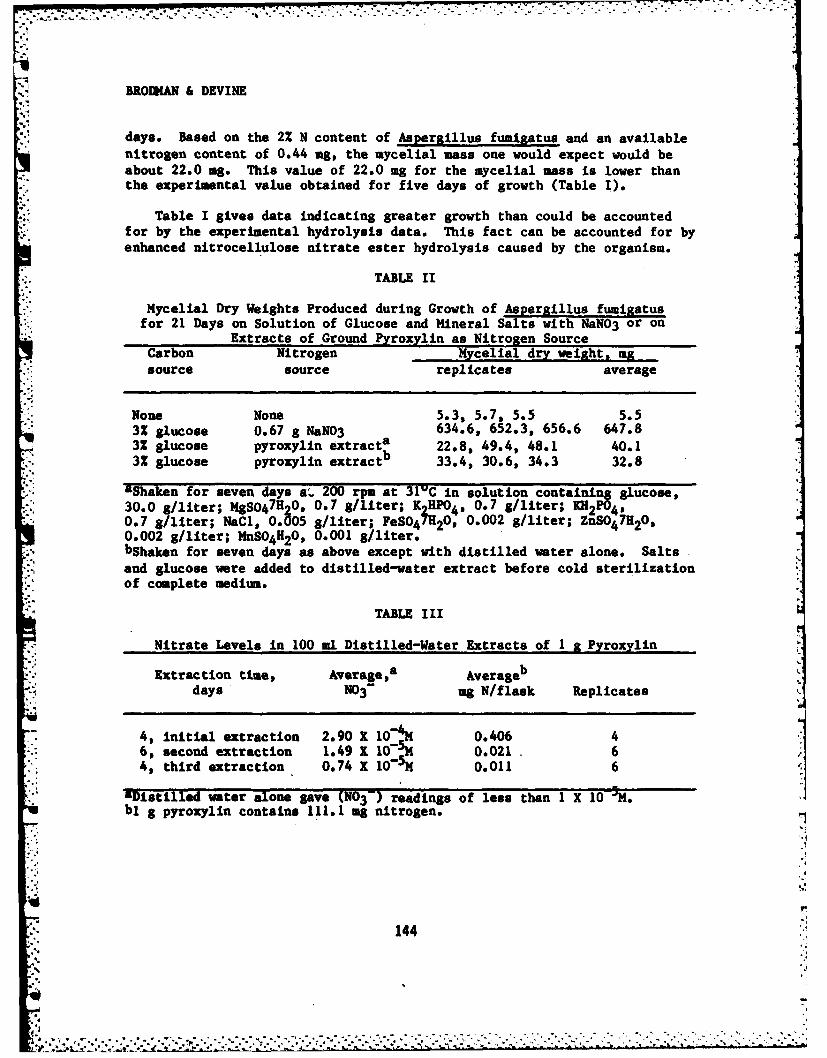
-* . . - -
BROWKAN & DEVINE
days. Based on the 2% N content of Aspergillus fumizatus and an availablenitrogen content of 0.44 mg, the mycelial mass one would expect would beabout 22.0 mg. This value of 22.0 mg for the mycelial mass is lower thanthe experimental value obtained for five days of growth (Table I).
Table I gives data indicating greater growth than could be accountedfor by the experimental hydrolysis data. This fact can be accounted for byenhanced nitrocellulose nitrate ester hydrolysis caused by the organism.
TABLE II
Mycelial Dry Weights Produced during Growth of Aspergillus fumigatusfor 21 Days on Solution of Glucose and Mineral Salts with NaNO3 or on
Extracts of Ground Pyroxylin as Nitrogen SourceCarbon Nitrogen Mycelial dry weight, tgsource source replicates average
None None 5.3, 5.7, 5.5 5.53% glucose 0.67 g NAN03 634.6, 652.3, 656.6 647.83Z glucose pyroxylin extracta 22.8, 49.4, 48.1 40.13% glucose pyroxylin extractb 33.4, 30.6, 34.3 32.8
- aShaken for seven days a. 200 rpm at 31C in solution containing glucose,"" 30.0 g/liter; MgS047H20, 0.7 g/liter; K2HPO4, 0.7 g/liter; 2 4.
* '* 0.7 g/liter; NaCI, 0.005 g/liter; FeS047H20! 0.002 g/liter; ZnS04 7H20,0.002 g/liter; MnS04H20, 0.001 g/liter.bShaken for seven days as above except with distilled water alone. Salts
-* and glucose were added to distilled-water extract before cold sterilizationof complete medium.
TABLE III
Nitrate Levels in 100 ml Distilled-Water Extracts of I aPyroxylin
Extraction time, Average,a Averageb
days NO3- mg N/flask Replicates
4, initial extraction 2.90 X 10- 0.406 46, second extraction 1.49 X 1O M 0.021 64, third extraction 0.74 X 10-. 0.011 6
aDistilled water alone gave (N03-) readings of less than 1 X 10 .bl g pyroxylin contains 111.1 mg nitrogen.
144
0-1
aROOMAN & DEVINE
In summary, it has been shown that Aspergillus fumigatus can utilize nitro-gen from pyroxylin suspended in a nitrogen deficient medium if a supple-mentary carbon source is provided. It appears that the organism does notdirectly attack the nitrocellulose but rather utilizes the nitrogen result-ing from the hydrolysis of the nitrocellulose nitrate eater group. Further,it appears that the organism caused enhanced hydrolysis of the nitrocellu-lose.
I
REFERENCES
1. B. W. Brodman, M. P. Devine, and M. T. Gurbarg, J. Appl. Polym. Sci.,18, 943 (1974).2. Be. W. Brodman, M. P. Devine, R. W. Finch, and M. S. MacClaren, J.Appl. Polym. Sci., 18, 3739 (1974).3. B. W. Brodman, J. A. Sipia, Jr., and So Schwartz, J. Appl. Polym. Sci.,19, 1905 (1975).4. T. Bokorny, (as quoted by T. Urbanski) in Chemistry and Technology ofExplosives, Vol. 2, Pergamon, London, England, 1965, p. 313.5. B. Malenkovic, (as quoted by T. Urbanski) in Chemistry and Technologyof Explosives, Vol. 2, Pergamon, London, England, 1965, p. 313.6. M. Jacque, (as quoted by T. Urbanaki) in Chemistry and Technology ofExplosives, Vol. 2, Pergamon, London, 1965, p. 313.7. T. M. Wendt and A. H. Kaplan, Treating Waster Water Containing Cellu-lose Nitrate Particles, U.S. Pat. 3,939,068 (Feb. 17, 1976).8. J. Desmaroux, (as quoted by T. Urbanski) in Chemistry and Technologyof Explosives, Vol. 2, Pergamon, London, England, 1965, p. 397.
3.45,.4
?. . .,. . . . . . . . . . .
.- . . .. . . . . . . . . ..,
BROWN
AN EMPIRICAL MODEL FOR NEAR MILLIMETER WAVESNOW EXTINCTION AND BACKSCATTER (U)
*Douglas R. Brown, Ph.D.
US Army Atmospheric Sciences LaboratoryWhite Sands Missile Range, New Mexico 88002
A snow extinction and backscatter model for near millimeter waveswas developed to complete a set of natural atmosphere propagation modelsfor inclusion in the Electro-Optics System Effects Library (EOSAEL)(1). This model is compact, simple, fast, and uses commonly availablemeteorological data as inputs. The accuracy is commensurate with theaccuracy of those Input parameters; where the input parameters do notproperly characterize the environment, further input specification isavailable. For snow, the rain equivalent accumulation rate is the funda-Mental input, with air temperature providing the distinction between dryand wet snowtypes. For millimeter wave (MW), the classification of thesnowflake by Its ice-to-liquid-water ratio Is necessary, due to the largedifferences in the complex indices of refraction of ice and water (2).
The snow extinction model is presented first, Including a review ofthe data used to generate It. The backicatter model is then discussed,followed by a comparison between the model and measurements made at theCold Regions Research and Engineering Laboratory (CRREL) SNOW-ONE test inJanuary-February 1982 (3).
1. SNOW EXTINCTION
While the literature on the interaction of MMW with snow is limited,the complete literature will not be reviewed here; a general review hasbeen carried out by Kobayashi (4). only those results used In the modelwill be discussed.
The general classification of snowtypes is discussed in detail byNishitmuji (5). Four types are described: dry, moist, vet, and watery,distinguished by the density of the snowflake. Because no other determi-nation of snowflake density was reported in the literature, it is diffi-cult to follow this classification procedure; in practice, snowtypes were
147
.. -- . , . .
".-. .O.
BROWN
inferred by comparison with the Nishitsuji extinction results where pos-sible. Data for extinction by wet snow at 15 0Hz, moist snow at 35 CHz,and watery snow at 50 0Hz are presented. A Hie scattering type model wasdeveloped by Nishiteuji, but is cumbersome, and only his experimentalresults were employed.
r..Data at 11, 15, 24, and 48 0Hz are presented by Oomori and Aoyagi
(6), although no indication of the snowtypes is given. A unique confocalresonator was used to measure snow attenuations. Comparison with otherdata seems to indicate that moist snow propagation was measured. Thedata are modeled with an aR relation, which is derived using a theory ofsnowfall statistics and in which R is rain equivalent snowrate and a andb are parameters. The a parameter data agrees well with other data, butat 24 and 48 0Hz there is poor agreement for the b parameter.
Moist snow data is provided at 35 0Hz by Robinson (7). The data setis of limited extent, having only seven useable values. Halinkin et al(8) measured dry snow at 35 0Hz, with but a slight improvement: eightpoints.
Only two data points exist in the literature for frequencies above50 0Hz: one at 140 0Hz for wet snow by Richard, Kammerer, and Reitz (9),and one at 312.5 0Hz for dry snow by Babkin et al (10). The Richardpaper also reports visual range for the same snow data. Readers shouldnote the error in reference (9), figure 25, where the a parameter iswritten as 1.37 but clearly should be 3.7 Instead.
Analysis of the data shows that an aRb relation for snow is thesimp.est form for a snow model, but does such a model have theoretical
"%' foundations? A review of A1b models for rain extinction provides theguidelines.
Relations of the form asb can be derived for rain in the Rayleighand optical limits. This result relies on the use of negative exponen-tial or modified gamma dropsize distribution and a power series represen-tation for the particle forward scattering amplitude. Where such powerseries representations cannot be found, direct fits to Mte scatteringcalculations are used. Such models provide highly accurate results foronly a limited range of rainrates, but application over wider ranges isuseful because of the general dominance of errors introduced from thebeginning by the arbitrary raindrop size distribution. Errors can be
significant, but may be minimized by the Judicious selection of raindropdistribution (11).
148
... . . . .. -... . ..: , -- d d " - -
s M ammn"r : d ". . . .. *..
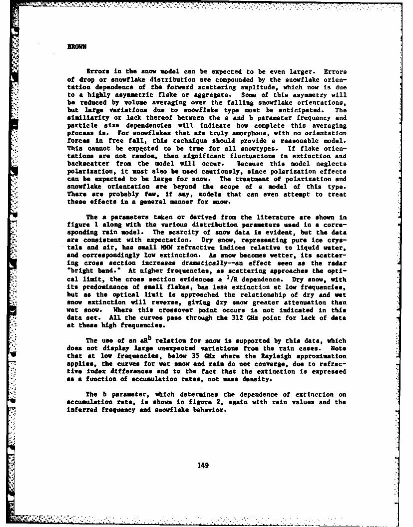
. ... 2%' e.t . * *, . .- . t . . . . . , . m m
BROWN
Krrors in the snow model can be expected to be even larger. Errorsof drop or snowflake distribution are compounded by the snowflake orien-tation dependence of the forward scattering amplitude, which now is dueto a highly asymmetric flake or aggregate. Some of this asymmetry willbe reduced by volume averaging over the falling snowflake orientations,but large variations due to snowflake type must be anticipated. The
*siailiarity or lack thereof between the a and b parameter frequency andparticle size dependencies will indicate how complete this averagingprocess is. For snowflakes that are truly amorphous, with no orientation
"* forces in free fall, this technique should provide a reasonable model.This cannot be expected to be true for all snowtypes. If flake orien-tations are not random, then significant fluctuations in extinction andbackscatter from the model will occur. Because this model neglectspolarization, it must also be used cautiously, since polarization effectscan be expected to be large for snow. The treatment of polarization andsnowflake orientation are beyond the scope of a model of this type.There are probably few, if any, models that can even attempt to treatthese effects in a general manner for snow.
The a parameters taken or derived from the literature are shown infigure 1 along with the various distribution parameters used in a corre-sponding rain model. The scarcity of snow data is evident, but the dataare consistent with expectation. Dry snow, representing pure ice crys-tals and air, has small MKW refractive indices relative to liquid water,and correspondingly low extinction. As snow becomes wetter, its scatter-ing cross section increases dramatically--an effect seen as the radar"bright band." At nigher frequencies, as scattering approaches the opti-cal limit, the cross section evidences a 1/R dependence. Dry snow, withits predominance of small flakes, has less extinction at low frequencies,but as the optical limit is approached the relationship of dry and wetsnow extinction will reverse, giving dry snow greater attenuation thanwet snow. Where this crossover point occurs is not indicated in thisdata set. All the curves pass through the 312 GHz point for lack of dataat these high frequencies.
The use of an ai b relation for snow is supported by this data, whichdoes not display large unexpected variations from the rain cases. Notethat at low frequencies, below 35 GHz where the Rayleigh approximation
* applies, the curves for wet snow and rain do not converge, due to refrac-tlve index differences and to the fact that the extinction is expressedas a function of accumulation rates, not mass density.
The b parameter, which deterines the dependence of extinction onaccumulation rate, is shown in figure 2, again with rain values and theinferred frequency and snowflake behavior.
149
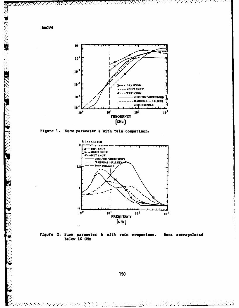
I IJ I I !l J Iq ,,I J , |.n IP - , u. ,- -.. , . - , ,, .. : , - ,, ;-. - . - . , . - o.
BROWN
10'
100
,10"2 --- DRY SNOW"'-'" --- MOIST SNOW
- d- -- WET SNOW1-3 JOSS TIFVNDERSTORM
-. MARSHALL- PALMER
10,- "8 JOSS DRIZZLE
10o l0 102 103
FREQUENCY
[GeZ]
Figure 1. Snow parameter a with rain comparison.
I PARAMETER
•0--- IRY SNOWx- -- MOIST SNOWdA---WET SNOW
- JOSS TIIUNDERSTORM
1.5 - JOSS DRIZZLE
loll 0o1FREQUENCY
(mHzj
Figure 2. Snow parameter b with rain comparison. Data extrapolatedbelow 10 GOz
150
The wet and moist snow data are similar to the Jose thunderstorm andMarshall-Palmer behavior; these curves have been roughly followed indefining the wet and moist snow b parameter curves. Dry snow behavior isexpected to follow the Jose drizzle distribution due to the predominanceof small particles in both cases. However, two points provide only thecrudest indication of the dry snow behavior. The large peak value of thedry snow b parameter should not cause alarm, because dry snovrates aregenerally quite low, there being little or no data for rates above 2 mm/hin the literature.
Air temperature at the ground is used to determine the snowtype for* an extinction calculation. Dry snow is used at or below freezing, moist
snow parameters are used from 0C to 2C, and wet snow is employed above2'C. These temperatures are rough estimates, based upon the assumption
. that temperature lapse rates are negative and are subject to adjustmentdepending on the specific storm characteristics.
The frequency range covered by this model is not well defined. With*. eight data points defining three curves and with only two measurements
above 50 GHz, the high frequency behavior of the model is obviously sub-ject to error. For this reason, use of the model above 100 Mes should be
- accompanied with caution.
2. SNOW BACKSCATTER
MW snow beckscatter data is severly limited by the use of inferredreflectivity factors derived from meajured snowflake size dlstribu-tions. Such results are valid only in the Rayleigh regime below 35GRz. Initially, a Rayleigh model was employed with restricted frequencycoverage. With the publication of a datum at 95 GCz resulting from theSNOW-ONE measurements, it was decided, due to the inadequacy of theexisting model, to develop a new model using all the available data. Novalidation of this model is possible because all the data were incorpo-rated in it.
The similar behavior of the rain and snow a and b parameters led tothe use of the rain backscatter model to provide the shape of the snowbackscatter curves. This procedure can be dangerous, but theory andexperiment are not yet able to provide sufficient knowledge to 6afine anindependent model. At long wavelengths, the reflectivity factors of Imalat al (12) are used along with the Rayleigh relation to compute back-scatter cross section, n,
1 w1k1 2
': 151
,,.Z
".. . . -. f '" " "
BROWN
where k - (m2 - 1)/(u2 + 2), m is the complex index of refraction, A thewavelength, and Z = $ N(D)D6 dD where N(D) In the snowflake size distri-bution function. In practice, reflectivity Is related to rain equivalentsnowrate as
Z =mRb
Table 1 lists the values of the a and b parameters from Imal et al, wheretheir classification is assumed to correspond with our dry, moist, andwet classes.
TABLE 1.* RAYLEIGHI BACKSCATTER PARAMETERS
Snowtype a b
dry 600 1.8
moist 1800 1.8
wet 2400 1.8
At shorter wavelengths, the rain backscatter curve was forced to gothrough the datum from Nemarich et al (13) at 95 GHz. Their nine datapoints were abstracted into a single upper bound value. This was neces-sary because their data did not correlate well with the snow accumulationdata, an apparent example of snowflake resonant scattering variations.The value used was 6.6 x 10⁻⁵ m2/23 for a dry snowrate of 1 mn/h.Examples of the computed snow backscatter cross sections for the threesnowtypes and a snowrate of 5 m/h are shown in figure 3. Comparisonwith rain backscatter indicates that for dry snow the cross section Ismuch less for snow; for moist snow, rain and snow are comparable; and forwet snow, snow backscatter is much larger than rain.
In scaling the snowtype results, it was assumed that the Imai et alresults would hold at all frequencies, thus giving moist snow three timesand wet snow four times the dry snow cross section. This may not becorrect, but no data are available yet to improve the assumption.
3. MODEL EVALUATION
The SNOW-ONE test (3) of January and February 1981 provided thefirst opportunity to evaluate the snow extinction model using a totally
'U independent date set.
152
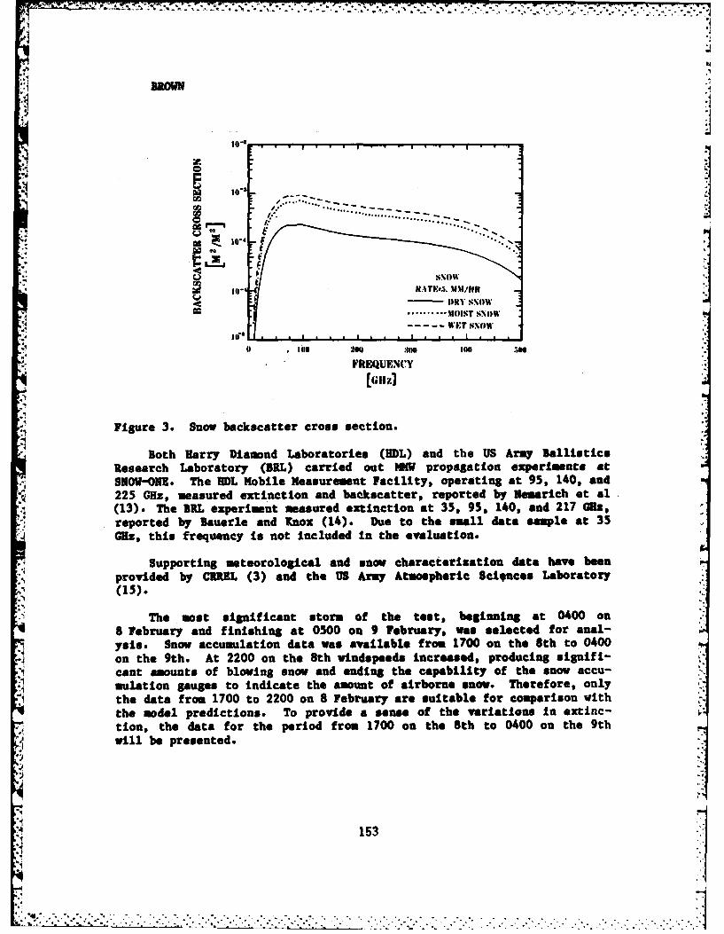
,o-
............
4t
SNE!~OW
.... .. O STS O
0 , lon :11HO 188lO 1
FREQUENCY
[Gilz]
Figure 3. Snow backscatter cross section.
Both Harry Diamond Laboratories (HDL) and the US Army BallisticsResearch Laboratory (BIL) carried out MW propagation experiments atSNOWONz. The HDL Mobile Measurement Facility, operating at 95, 140, and225 G0z, measured extinction and backscatter, reported by lemarich et al
(13). The ILL experiment measured extinction at 35, 95, 140, and 217 GEf,reported by Bauerle and Xnox (14). Due to the small data sample at 35GO., this frequency is not Included In the evaluation.
Supporting meteorological and snow characterisation data have beenprovided by CRUEL (3) and the US Army Atmospheric ScLqnces Laboratory
, ~(13).•.:( .The most significant storm of the test, beginning at 0400 on
8 February and finishing at 0500 on 9 February, was selected for anal-ysts. Snow accumulation data was available from 1700 on the 8th to 0400on the 9th. At 2200 on the 8th windspeeds increased, producing signifi-cant amounts of blowing snow and ending the capability of the snow accu-.ulation gauges to indicate the amount of airborne snow. Therefore, onlythe data from 1700 to 2200 on 8 February are suitable for comparison withthe model predictions. To provide a sense of the variations in extinc-tion, the data for the period from 1700 on the 8th to 0400 on the 9thwill be presented.
153
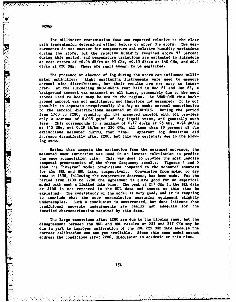
,,. . . . . . . . . .
BROWN
The millimeter transmission data was reported relative to the clearpath transmission determined either before or after the storm. The mea-surements do not correct for temperature and relative humidity variationsduring the storm, but the relative humidity remained above 95 percentduring this period, and temperature variations are estimated to introduceat most errors of *0.06 dB/km at 95 GHz, *0.15 dB/km at 140 GHz, and *0.4dB/km at 220 GHz. These are small enough to be neglected.
The presence or absence of fog during the storm can influence milli-meter extinction. Light scattering instruments were used to measureaerosol size distributions, but their results are not easy to inter-pret. At the succeeding SNOW-ONE-A test held in Dec 81 and Jan 82, abackground aerosol was measured at all times, presumably due to the woodstoves used to heat many houses in the region. At SNOW-ONE this back-ground aerosol was not anticipated and therefore not measured. It is notpossible to separate unequivocally the fog or smoke aerosol contributionto the aerosol distributions measured at SNOW-ONE. During the periodfrom 1700 to 2200, equating all the measured aerosol with fog providesonly a maximum of 0.035 gm/m3 of fog liquid water, and generally muchless. This corresponds to a maximum of 0.17 dB/km at 95 0Hz, 0.24 dB/kmat 140 GHz, and 0.29 dB/km at 220 GHz, all less than 10 percent of theextinctions measured during that time. Apparent fog densities didincrease dramatically after 2200, but this was certainly due to the blow-ing snow.
Rather than compute the extinction from the measured snowrate, themeasured snow extinction was used in an inverse calculation to predictthe snow accumulation rate. This was done to provide the most concisetemporal presentation of the three frequency results. Figures 4 and 5show the "inverse" model predictions compared to the measured snovratefor A',e BRL and HDL data, respectively. Conversion from moist to drysnoa at 1850, following the temperature decrease, has been made. For theperiod from 1700 to 2200 the agreement is quite good for an empiricalmodel with such a limited data base. The peak at 217 CHz in the IRL dataat 2100 is not repeated in the HDL data and cannot at this time be
" explained. The consistency of the model is very good, and it is temptingto conclude that the snow accumulation measuring equipment slightly
undersamples. Such a conclusion is unwarranted, but does indicate thattraditional snowrate measurements are really not adequate for thedetailed characterization required by this data.
The large excursions after 2200 are due to the blowing snow, but the
disagreement between the HDL and BRL results at 225 and 217 GHz may bedue in part to improper calibration of the HDL 225 CHz data because thecorrect calibration was not yet available. Since this snow model cannotaddress the conditions after 2200, discussion Is academic at this time.
154
, ~~.. •.. .... ... ,.. -. ... -..... .- .-. .,..- "- " .' " " ,.,. ',." ", ,- . ,
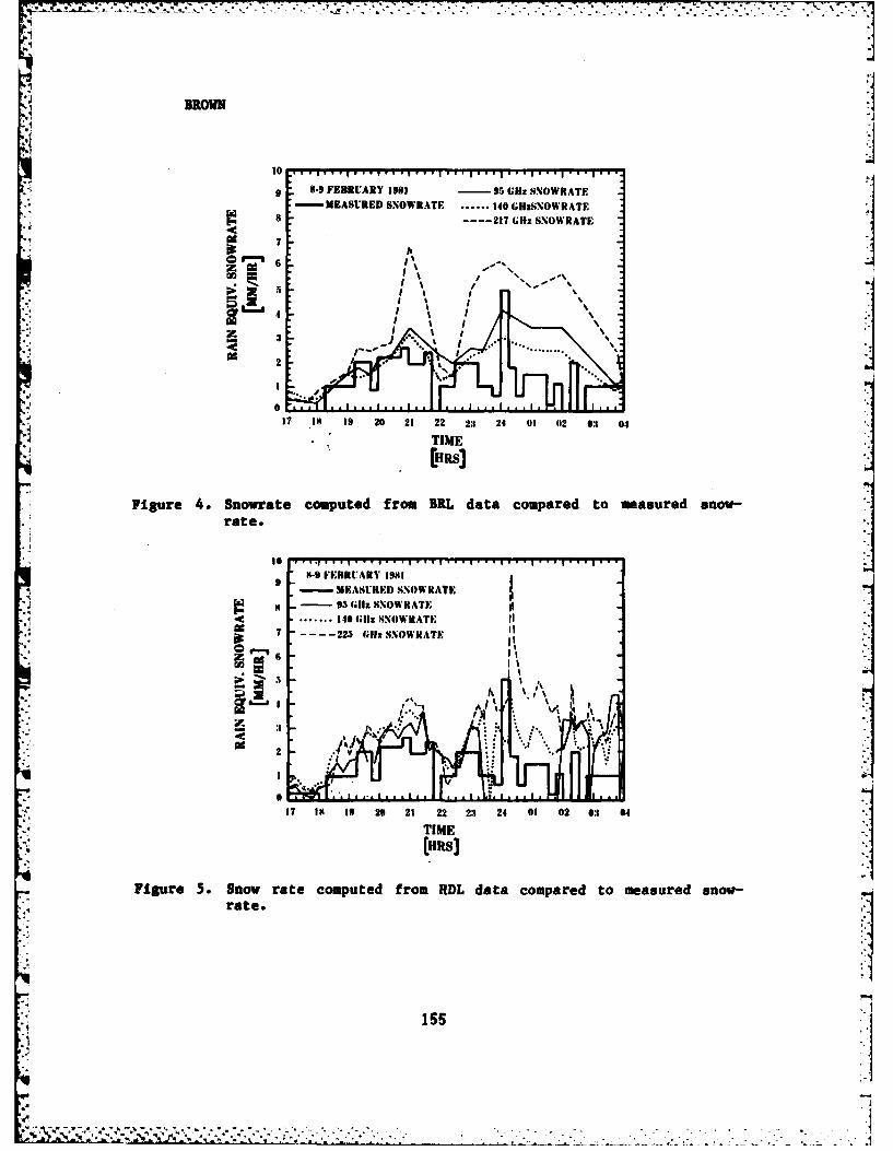
BROWNj
* 8-9 FEBRUARY 1981 - 95 Gflz SNOWRATE-MEASURED SNOWRATF .... 140 GHzSNOWRATE
8 --- 217 ~i SNWEAT
4 AT
z m6
P7.:I 2 2 2 2 4 I 0 3 S5 16"TIME
3HS
*1 9 ~- MESRDSORTE
Figur~4 le 4. Sortecmutdfo SORAT aacmardt esue nw
7 - -22H 9.51 SOWRATF,- 5 .1.H%'RT
C . ... ,0Gi NN* *T
I7 1 9 2 1 2 3 2 1 0 3 0---22 (1lSNWRTIM
[ms
Figre .Sowrat copued romRD daa cmpredto mesurd sowrate
TIME

BROWN
These results give added confidence to the use of the model at fre-quencies up to 225 OHz, at least for dry snow. Wet and mol. - snow accu-racy must still be determined at these high frequencies. C .-n existingfield test programs, it is unlikely that measurements above 275 GHz willbe available, so that extension of the model with confidence above thisfrequency may not be possible.
4. CONCLUSION
b A new MMW snow model has been presented, based upon the use of an
aRb relation. The data used in its development were briefly reviewed,and the similarity of the snow and rain models was shown. The extinctionmodel was compared with independent data from two separate facilities anddemonstrated remarkably good agreement. The backscatter model could notbe evaluated because no independent data exist.
The development of this model has clarified three data deficien-cies: lack of snow backscatter data from all types of snow, lack ofpolarized propagation data at all frequencies, and lack of unpolarizeddata at frequencies above 100 GCs. Efforts to provide for the Inadequa-cies of the data base continue, but snow data is difficult to obtain, andfurther development of the model will be slow.
A particular problem is that a large data base is necessary at eachfrequency to define the a and b parameters, due to the use :.f snowrate asthe fundamental quantity. This also limits the model to near calm condi-tions, since there is no way to estimate the effects of blowing snow. Amore sophisticated model using airborne snow density or the snowflakesize distribution function itself could be developed, but the data setwould be even smaller than that employed here. Since these data are notpart of the standard meteorological data base, it would be most difficultto apply such Adels over various geographic and diverse climatologicalareas. For these reasons, this empirical MMW snow extinction and back-scatter model is offered as a solution to the predictive problem of theeffects of snow on MMW propagation.
5. REFERENCES
1. Duncan, Louis D., EOSAEL 80, Volume 1, Technical Documentation,ASL-TR-0072, US Army Atmospheric Sciences Laboratory, White Sands MissileRange, New Mexico, 1981.
2. Ray, P. S., "Broadband Complex Refractive Indices of Ice and Water,"Applied Optics, 11:1836-1844, 1972.
..16
40156
3. Redfield, R. K., ed., SNOW-ON Preliminary Data Report InternalReport #715, US Army Cold Regions Research and Engineering Laboratory,Hanover, New Hampshire, 1981.
4. Kobayashi, Herbert K., Effect of Hall, Snow, and Melting Hydrometeorson Millimeter Radio Waves, ASL-TR-0092, US Army Atmospheric SciencesLaboratory, White Sands Missile Range, New Mexico, 1981.
5. Iishitsuji, A., "Method of Calculation of Radio-Wave Attenuation in-7; Snowfall," Elect and Comm in Japan, 54-B:34, 1971.
6. Oomori, T., and S. Aoyagi, "A Presumptive Formula for Snowfall Atten-uation of Radio Waves," Elect and Comw in Japan, 54-3:74, 1971.
7. Robinson, N. P., "Measurements of the Effect of Rain, Snow, and Fogson 8.6 m Radar Echoes," Proceedings IE, 203-3:209, 1955.
8. Mahlinkin, V. G., et al, "Attenuation of Signal at the WavelengthX - 8.6 m in Hydrometeors," Red Eng and Elect Physics, 21:1, 1976.
9. Richard, W. W., J. E. Kaimerer, and R. G. Reitz, "140-GHz Attenuationand Optical Visibility Measurements of Fog, Rain, and Snow," MemorandumReport ARBRL-MR-2800, US Army Ballistics Research Laboratory, AberdeenProving Ground, Maryland, 1977.
10. Babkin, Yu. S., et al, "Attenuation of Radiation at a Wavelength of0.96 - in Snow," Radio Eng and Elect Physics, 15:2171, 1970.
11. Keizer, W., J. Snieder, and C. de Haan, "Rain Attenuation Measure-ments at 94 GHz: Comparison of Theory and Experiment," DPP Symposium,Neubiberg bei Munchen, Germany, 1978.
12. Imai, I., M. Fujiwara, I. Ichimura, and Y. Toyama, "Radar Reflec-tivity of Falling Snow," Meteorology and Geophysics (Japan), 6:130, 1955.
13. Nemarich, J., R. J. Wellman, D. Rocha, and G. D. Wetuet, "Character-istics of Near-Milliseter Wave Propagation in Snow," SPI , Vol 305, inpress.
14. Bauerle, D., and J. E. Knox, "Mill1metre Wavelength Radar Propaga-tion and Backscatter Measurements at SNOW-ONE," Snow Symposium I, inpress.
15. Olsen, R. 0., D. R. Brown, J. E. Butterfield, and R. Orkasinski,"SNOW-ONE Atmospheric and Transmission Measurements," Snow Symposium I,in press.
157
,
Bushell, Manriquez, Merkel, & Scharf
AURORA FLASH X-RAY FACILITYAS A SOURCE-REGICHI EMP SIMULATOR
M. Bushell, R. Manriquez,G. Merkel, and *W. D. Scharf
US Army Electronics Research andDevelopment Command
HARRY DIAMCND LABORATORIESAdelphl, MD 20783
The study of source-region electromagnetic pulse phenomenology andcoupling "4 is distinguished from more conventional electromagnetic researchby the presence of time-varying air conductivity. The relevant Maxwellequations are:
VH = 0 ,
VxE =-lMVxH - J + GE + e:
These can be combined into a wave equation for the electric field:V 2 -"(e + A + ;Z) + V(p/e)
(The magnetic field can be found by time-integrating VxE.) The first twoterm appear in the well-known homogeneous wave equation:
22 2E - 0
2 2 at2
where c --
The third term represents the dissipation of energy resulting from airconductivity--i.e., the collision of charged free carriers (electrons andheavy ions) with neutral molecules. When this term dominates the second, thesystem becomes overdauped and is described by the diffusion equation:
2 aR;.'-V E - tic 2 --- = 0
The fourth term contributes only when a is time-varying, and even then is* significant only when the time variation is as fast or nearly as fas as that
of (t) . (Note that the third and fourth terms together represent (OE)--the time derivative of conduction current density.) at
The right-hand side terms represent the electromagnetic sources. In the
1.59
Bushell, Manriquez, Merkel, & Scharfcase of nuclear E33, these sources are provided by high energy radiation froma nuclear device--through the mechanism of the Compton effect (which leads tospace curent and charge separation)--and by current and charge density inducedin local or distant objects (including the ground). The region in which5(x,t) and p(xt) are non-zero is called the source region, and the term
"souce-region Z3P* is used whenever these local drivers are significant. In a*: typical burst, the source region may be several miles in linear extent, and
sources throughout the region contribute, through the well-known mechanisms ofelectromagnetic radiation and diffusion, to the fields at any given point.
This last observation lies at the heart of the greatest challenge tosuccessful SREMP simulation. Powerful sources of high-energy pulsed radiation(e.g., AURORA 5 '6 , and Hermes 7 ' 8 ) are available, and these naturally produce
Iradiation is released. There is a temptation to assume that if these localsources are reasonably well reproduced, the full electromagnetic environmentwill be also. This naive assumption neglects the contribution of "distant"sources that cannot be reproduced, since existing pulsed-radiation technologyis capable of irradiating a volume whose linear dimensions are expressed intens of meters at most. (The AURORA test cell measures 20 m x 12 m x 5 m.)
W Of course, due to the finite velocity of light, the "prompt" environmentcan be reliably reproduced. However, after 10 nanoseconds or so, the absenceof sources at a distance of more than 20 feet from the field point becomesnoticeable. In addition, if the simulation testing is performed in a volumeenclosed by metal walls (as in AURORA), this effect is aggravated by theelectromagnetic boundary conditions imposed by these walls. They short outthe electric field. Figure I compares (not to scale, but schematically) theAURORA test cell volume to the vast distribution of Compton electron sourcecurrents in an actual SREMP. Figure 2 is a schematic view of the inside ofthe AURORA test cell during a shot.
A less subtle limitation of facilities like AURORA is that the radiationpulse itself does not faithfully reproduce the pulse produced by a nuclearweapon. It rises more slowly and decays more quickly. The gamma spectrum isnot quite right. The late-time drivers are very different, largely due to thelack of neutrons.
In spite of these limitations, the authors, who have for several years4been conducting an experimental program at AURORA, 9 2 7, have found that usefuland relevant work can be done there. AURORA is a fine source of "basicphysics" data on SREMP environments and coupling. Further, we believe thattesting of the nature described here should be incorporated in any plan for8R1NP vulnerability assessment and hardness validation of military andcivilian electrical and electronic equipment. While ultimate determination ofvulnerability and hardness will rely also on computer calculations, we feelthat AURORA testing plays an essential role, both in validating the codes andin exposing unexpected vulnerabilities.
.RENP environments can, in a roug way, be described as belonging to one
160

In* t ... . . . . . i ,i .
-i
Bushell, anriquez, Merkel, & Scharf
!m~ .wm Nowayi ,111. ~NII li~e aM11l
*gzNq UII IATI
" / a
:i /"
Figur 1.Cmaisno,,,lvlm o h UORAtetCol ih h
k vast distribution (several iles diameter) of Compton current drivers-. I n ac tual SlllMP. Actually, the rlaive size of the test call is
. : much smaller than shown In the figure.
I -
SAUMMNA FFETSau~ mu
smg-ucsie aLnUshoNERn in t* r *., .I " r
LW EXW-."- OilLli Il)AtSS'
-, V OLUnM aw
Figure 2. Schematic view of the AURORA test cell during an AURORAshot. The metallic test cell walls can short out the electric fieldgenerated by the Compton electrons.
161
i"
4.5 1".
Bushell, Manriquez, Merkel, & Scharf
of two categories--tactical or strategic. These two types of environment, and
several approaches to their simulation, will be discussed in turn.
The Tactical Case
Tactical source-region EDP is the electromagnetic component of a nuclearenvironment in which a soldier can reasonably be expected to remain alive andfunctioning for a useful time. Thus, tactical equipment, for use in abattlefield, is typically hardened only to a level consistent with a "man-survivability criterion." In practice, this normally means that peakconductivity levels of more than 10 mho/m are of no interest. (Long cables,which may channel energy from the "deep source region" out to a less highlydosed area, is an exception to this general rule.)
Some rough indication of the time evolution and magnitudes of relevantparameters in the tactical case is given by the graphs of figure 3. These are
. taken from calculations made using LEMP 2 8 (a highly respected environment codein general use by the EMP community) and assuming a set of devicecharacteristics29 which describe no existing weapon, but can be taken as
:-- typical.
The primary driver is, of course, the dose rate, y , expressed in unitsof rads/s. Thus the j pulse shape determines the shapes of all relevant timehistories--i.e., S(xt), a(x,t), i(x,t), and A(x,t)
In early time, the most significant descriptive parameter is the 10%-90%risetime. This rise time, typically on the order of 10 nanoseconds, iscritical to the efficiency of resonant coupling to relatively small objects,with linear dimensions of ten feet or so. Most Army equipment (such asradios, vehicles, shelter-resident fire control systems, etc.) falls into thiscategory.
'- . In late time, the pulse can be described by one or more exponential decay"0 constants. These decay times are much longer than the risetime. At late
time, the resonant behavior of "small" objects is not relevant, and suchobjects can be regarded with considerable accuracy as simple currentcollectors--driven directly by a combination of oompton and conductioncurrent. (Displacement curent, important at early time, is of practically nosignificance at late time.)
Such "small" objects are ideally suited for testing in a facility such asAURORA. They can easily be transported to, and mounted in, the test cell.However, the limitations discussed earlier--the slow pulse rise and fast pulse
' decay--make certain coupling behavior impossible to observe using AURORA inits conventional, unmodified state. The authors have, however, greatlyenhanced the usefulness of AURORA for such small-object testing by introducinginto the test cell auxiliary sources of electromagnetic excitation.18 Forvery small objects, this may simply take the form of a pair of thin aluminumplates to which a high-voltage pulse is applied (fig. 4). In this way, theproper electric field is reproduced in the enclosed volume, and the AURORA
162
•- -
Bushell, Manriquez, Merkel, & Scharf
pulse serves the function of producing the radiation-induced conductivity andCompton current. The plates are made of aluminum foil in order to minimizeshielding, space-charge effects, and other evidences of interaction betweenthe radiation pulse and the auxiliary simulator. If the proper electric fieldis reproduced in this way, useful coupling measurements can be made on smallsystems--measurements which include the effects of time-varying' airconductivity. (The conductivity pulse, though it cannot precisely reproducethe threat conductivity pulse, does (1) permit the experimenter to learn moreabout the "basic physics" of such interactions, and (2) provide a test bed forvalidation of theoretical techniques--both analytical and numerical--forpredicting SREMP response of simple geometric forms, and, most importantly, ofsystems .)
In undertaking a simulation such as the one described above, one musttake care to maintain control over the environment by minimizing anyinteraction between the conductivity pulse and the auxiliary simulator. Inthe parallel-plate structure described above, the interaction mechanism issimply that the radiation produces a conductive path across the plates--i .e.,a time-varying conductance appears in parallel with the capacitancecharacterizing the simulator structure. This time-varying conductance has thevalue:
G(t) C(t)
where C is the plate capacitance. One can ensure that the appearance of this:-" shunting conductive path produces only minimal distortion of the driving
electric field seen between the plates, by incorporating into the structure a" low-value resistor, R, such that:
Cymax
(See figure 4, where the 10-9 resistor serves this purpose.)
The authors have used the approach described above, using two 8' x 4'aluminum foil plates separated by 2 ft, to excite a helical slow-wavestructure intended to model a long cable or wire over ground. A 100-kV, 20-nsrise time, 2-ljs fall-time pulser (built by Pulsar) was used to drive thesystem. The behavior of the simulator was monitored by a number of currentsensors, by two single-ended Z-field sensors mounted on the grounded plate,
*and by a balanced sensor suspended between the two plates.
Of course, the parallel-plate structure is in fact not a capacitor, buthas some transmission-line characteristics. For the small simulator describedabove, these can reasonably be neglected, but for the testing of largerobjects a larger structure is required. Work has been done in AURORA using a
10-m-long (3-m plate separation) structure,17'18 whose inductive behavior
cannot safely be ignored (fig. 5) . The circuit of figure 6 is a moreappropriate approximation for this case. An example of the radiation-induceddistortion seen in such a structure is shown in figure 7 .
17 ,18 The inductance
163
*'-il
;" . " - . .• ,.* . ._ . - : .2
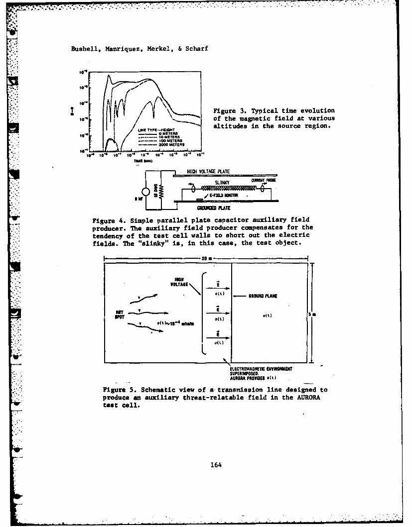
Bushell, Hanriquez, Merkel, & Scharf
so.
!lifl /'~\Figure 3. Typical time evolutionto-$ of the magnetic field at various
altitudes in the source region.1 - 0 METERS
-------------10 METERS100 METERS3000 METERS
HIG VOLTAGE PLATE
Figure 4. Simple parallel plate capacitor auxiliary fieldproducer. The auxiliary field producer compensates for thetendency of the test cell walls to short out the electricfields. The "slinky" is, in this case, the test object.
F ~~~~20 _________
MRN
VOI.TA6E0(t) - ROMl PLANEU
NOT ' MSPOT QW 0t) 5m
ELECTROMACNEII NVIRONMENTSUPiRINPOSED.AURORA PROVOES a(t)
Figure 5. Schematic view of a-transmoission line designed toproduce an auxiliary threat-relatable field in the AURORAtest cell.
164
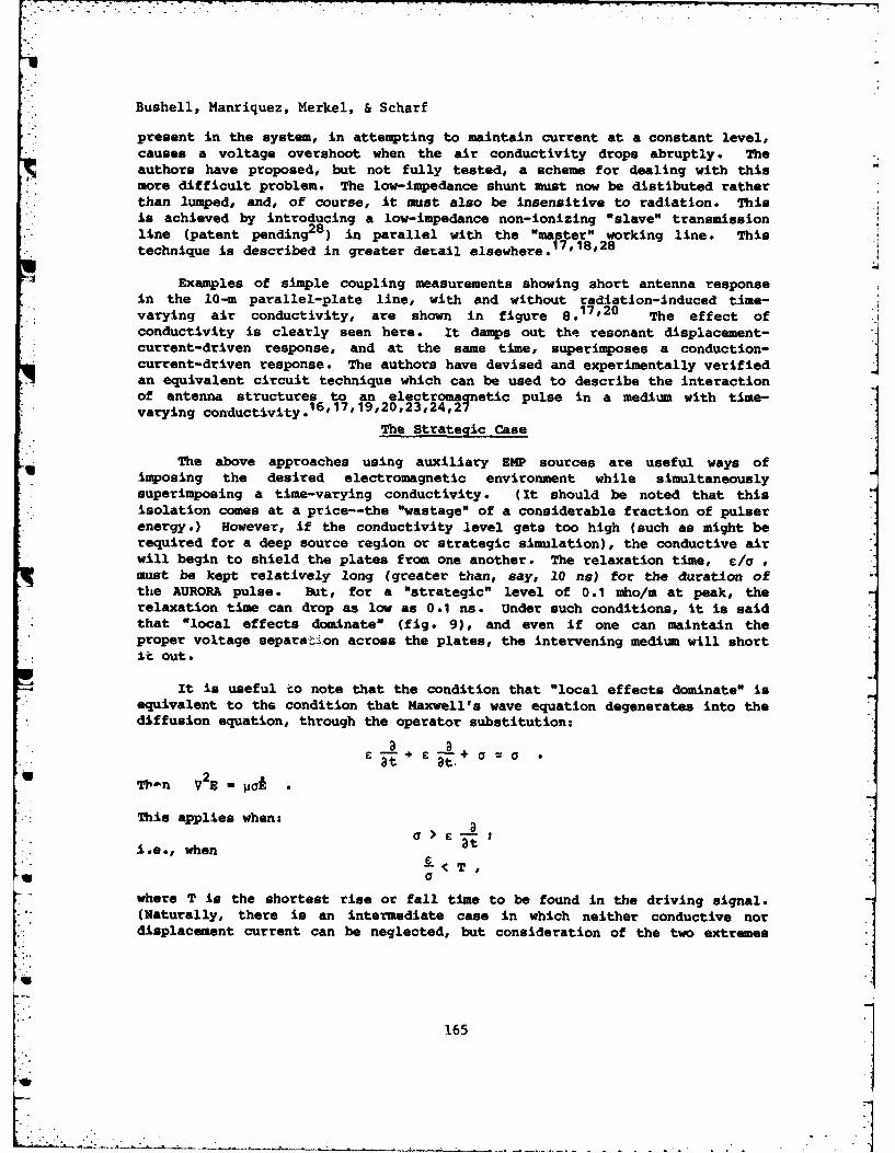
Bushell, Manriquez, Merkel, & Scharf
present in the system, in attempting to maintain current at a constant level,causes a voltage overshoot when the air conductivity drops abruptly. Theauthors have proposed, but not fully tested, a scheme for dealing with thismore difficult problem. The low-impedance shunt must now be distibuted ratherthan lumped, and, of course, it must also be insensitive to radiation. Thisis achieved by introducing a low-impedance non-ionizing "slave" transmissionline (patent pending2 8 ) in parallel with the "master" working line. Thistechnique is described in greater detail elsewhere.17 '18'2 8
Examples of simple coupling measurements showing short antenna responsein the 10-m parallel-plate line, with and without radiation-induced time-varying air conductivity, are shown in figure 8.17,20 The effect ofconductivity is clearly seen here. It damps out the resonant displacement-current-driven response, and at the same time, superimposes a conduction-current-driven response. The authors have devised and experimentally verifiedan equivalent circuit technique which can be used to describe the interactionof antenna structures to an electromalnetic pulse in a medium with time-varying conductivity.
16 ,17,19,20 ,2 3 ,2 4,27
The Strategic Case
The above approaches using auxiliary EMP sources are useful ways ofimposing the desired electromagnetic environment while simultaneouslysuperimposing a time-varying conductivity. (It should be noted that thisisolation comes at a price--the "wastage" of a considerable fraction of pulserenergy.) However, if the conductivity level gets too high (such as might berequired for a deep source region or strategic simulation), the conductive airwill begin to shield the plates from one another. The relaxation time, lG ,-must be kept relatively long (greater than, say, 10 ns) for the duration ofthe AURORA pulse. But, for a "strategic" level of 0.1 mho/m at peak, therelaxation time can drop as low as 0.1 ns. Under such conditions, it is saidthat "local effects dominate" (fig. 9), and even if one can maintain theproper voltage separation across the plates, the intervening medium will shortit out.
It is useful to note that the condition that "local effects dominate" isequivalent to the condition that Maxwell's wave equation degenerates into thediffusion equation, through the operator substitution:
a a
Th-n V2E " PuaA
This applies when: a
i.e., when
T
where T is the shortest rise or fall time to be found in the driving signal.(Naturally, there is an intermediate case in which neither conductive nordisplacement current can be neglected, but consideration of the two extremes
1
i.165
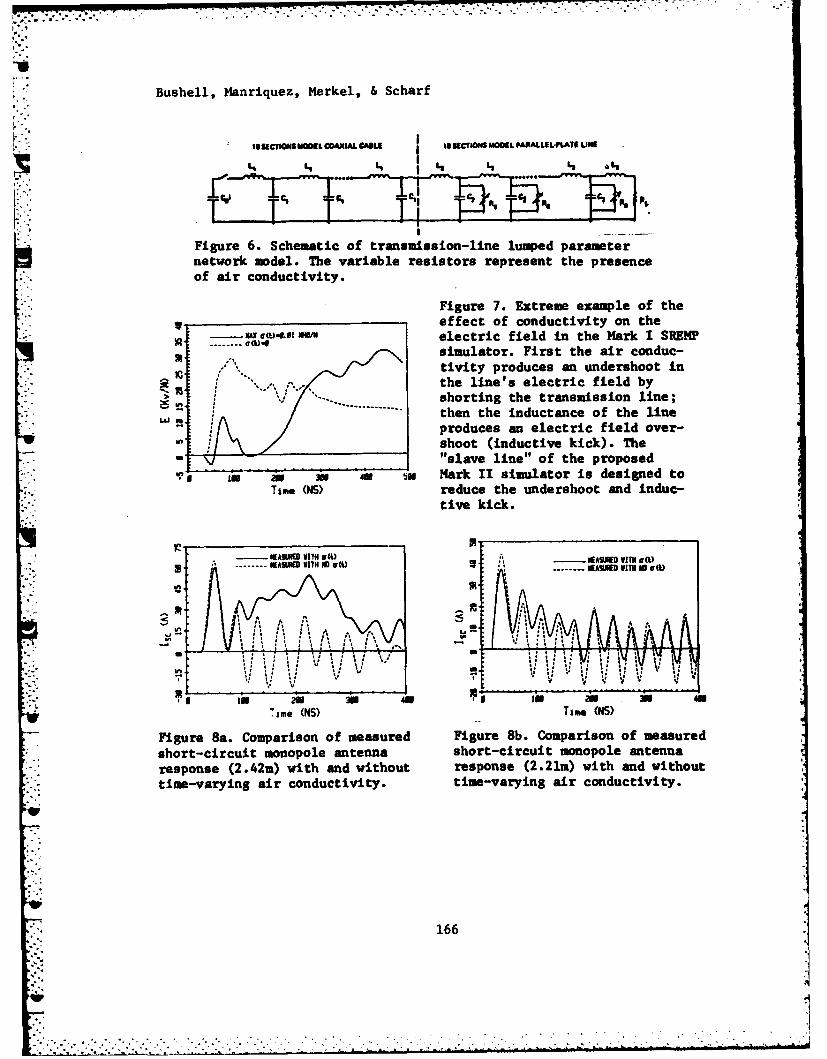
7 r-77.
.. 7 -7 -774
Bushell, Manriquez, Merkel, & Scharf
18SICT9W tIOOIL CAXIAL CANLE II Cr4MODEL FARALLEL-PLATE LINE
Figure 6. Schematic of transmission-line lumped paramternetwork model. The variable resistors represent the presenceof air conductivity.
Figure 7. Extreme example of theeffect of conductivity on the
S1 (U412 electric field in the Mark I S1REMsimulator. First the air conduc-tivity produces an undershoot inthe line's electric field byshorting the transmission line;then the inductance of the lineproduces an electric field over-shoot (inductive kick). The
\ "slave line" of the proposed2W~ an . 5H Hark 11 simulator is designed toTime WNS) reduce the undershoot and induc-
tive kick.
HEAW 11 I 04) NASM IED WW u~---- NEA9SM VIIN NOat ---- NEASI WIN NO V0
U,
-%"3A
7
. .. . ... ..
I ame (NS) Time (NS)
Figure 8a. Comparison of measured Figure 8b. Comparison of measuredshort-circuit monopole antenna short-circuit monopole antennaresponse (2.42m) with and without response (2.21m) with and withouttime-varying air conductivity, time-varying air conductivity.
166
Bushell, Manriquez, Merkel, & Scharf
* is useful for a qualitative understanding.)
When "local effects dominate," truly local drivers are needed to maintaina field. In the case of nuclear EMP, sustained Compton current performs thisfunction. In the AURORA, the authors, in collaboration with S. Graybill, K.Kerris, D. Whittaker and other AURORA staff members, have achieved this effectby using direct electron injection.
AURORA's five megajoules of stored energy appear at the vacuum diode as apulse of electron current. Ordinarily, a high-Z (usually tantalum) target isused to convert to x-ray energy. This is an inefficient process (assumingone's goal is to irradiate the test cell as heavily as possible) because:
(1) bremsstrahlung conversion efficiency at machine voltage is onlyabout 6%, the remaining energy being lost as heat in the target, and 1
(2) the x-ray range is on the order of hundreds of meters, so thatfurther energy is lost heating up the back wall.
If the target is removed and replaced with a 1/16th-in, steel vacuum-to-air interface, the electrons are released directly into the test cell andthese inefficiencies are avoided. There is no conversion loss, and theelectron ranges are of the order of the test cell length. Problems of self-consistent beam propagation (e.g., pinching and hosing) do not pose a threat,as has been determined in a series of AURORA experiments.
22
In addition to thorough mapping of the electron irradiation of the testcell in a number of diode configurations and commbinations, 2 2 couplingmeasurements have been made (by the authors) on aluminum cylinders, bothvertical and horizontal.2 3 Examples of these measurements are shown in figure10. Interpretation of the results is far from straightforward, since a numberof drive mechanisms contribute. The most important of these are:
(1) displacement current (early time),(2) conduction current,(3) Compton current, and
*(4) quasi-static space charge.
In addition to the higher irradiation of the room (as compared tobremsstrahlung-mode operation), the electron mode presents another significantbenefit. The rise time appears to be faster. Evidence for this is shown infigure 11, where dose-rate measurements--taken with a Cerenkov detector inelectron mode, and with a plastic scintillator in photon mode--are compared.
Conclusion
A good deal of thought and discussion is currently being generated onpossible designs for new SREMP simulation techniques. While this isundoubtedly a healthy development, the authors would like to stress that theAURORA facility remains a significant and ever improving source of data
167
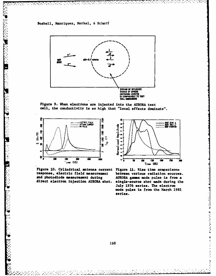
Bushell, Manriquez, Merkel, & Scharf
.- / a \HITI
-. \ /
-DOMAIN OF IWFLUENCERAMEUS OF SPHERE(DIFFUSION LEN TIH)IS COMPARAiLE TO TllCELL OWEN=
Figure 9. When electrons are injected into the AURORA teatcell, the conductivity is so high that "local effects dominate".
. ELECTR FIELD 1.- . 21 I------ 11 . .. ErMA CW"r I. .- -- . .
-~ ~ ~ ~ ~~t - iiIP WE----- WM
S
LL) 1)" ' ;, ". \ X
* t . '- . i.."-..._',
2 U 42 am U 800 ~ m m u mzme (NS) rimn (is)
Figure 10. Cylindrical antenna current Figure 11. Rise time comparisonsresponse, electric field measurement between various radiation sources.and photodiode measurement during AURORA gama mode pulse is from adirect electron injection AURORA shot. single-source shot made during the
li July 1976 series. The electronmode pulse is from the March 1981series.
168
i... -: :............f ",-,--- >i .. . . . . . . .
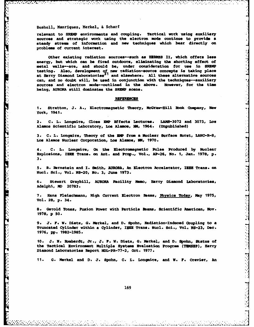
*. . - - : , , : ; . - *.- = . ' .. ." , '. . . L ..
., .". • -. - .. , - .
Bushell, Manriquez, Merkel, & Scharf
relevant to SREZkP environments and coupling. Tactical work using auxiliarysources and strategic work using the electron mode continue to provide asteady stream of information and new techniques which bear directly onproblems of current interest.
Other existing radiation sources--such as HERMES 11, which offers lessenergy, but which can be fired outdoors, eliminating the shorting effect ofmetal walls--are, and should be, under consideration for use in SUMWtesting. Also, development of new radiation-source concepts is taking placeat Harry Diamond Laboratories 3 1 and elsewhere. All these alternative sourcescan, and no doubt will, be used in conjunction with the techniques--auxiliarysources and electron mode--outlined in the above. However, for the timebeing, AURORA still dominates the SRDW scene.
REFERENCES
1. Stratton, J. A., Electromagnetic Theory, McGraw-Hill Book Oompany, New"- York, 194 1.
2. C. L. Longmire, Close DIP Effects Lectures. LANS-3072 and 3073, LosAlamos Scientific Laboratory, Los Alamos, NI, 1964. (Unpublished)
3. C. L. Longmire, Theory of the DIP from a Nuclear Surface Burst, LANC-R-8,Los Alamos Nuclear Corporation, Los Alamos, M, 1970.
. 4 . C. L. Longmire, On the Electromagnetic Pulse Produced by NuclearExplosions, IEEE Trans. on Ant. and Prop., Vol., AP-26, No. 1, Jan. 1978, p.
'i 3.
5. B. Bernstein and I. Sith, AURORA, An Electron Accelerator, INE Trans. onNucl. Sci., Vol. NS-20, No. 3, June 1973.
6. Stewart Graybill, AURORA Facility Memo, Harry Diamond Laboratories,Adelphi, ND 20783.
7. Hans Fleiscbmann, High Current Electron Beams, Physics Today, Nay 1975,SVol. 28, p. 34.
S.8 Gerold Yones, Fusion Power with Particle Beams, Scientific American, Nov."-: -1978, p 50.
9. 7. F. W. Dietz, G. Merkel, and D. Bpohn, Radiation-Znduced Coupling to aTruncated Cylinder within a Cylinder, IZE Trans. Nucl. Sci., Vol. NS-23, Dec.1976, pp. 1982-1985.
10. J. N. bRmbardt, Jr., J. F. W. Diets, G. Merkel, and D. Spohn, Status ofthe Tactical Environment Multiple Systems Evaluation Program (TENSEP), HarryDiamond Laboratories Report HDL-PR-77-2, Oct. 1977.
11. G. Merkel and D. J. Spohn, C. L. Longmire, and W. F. Crevier, An
169
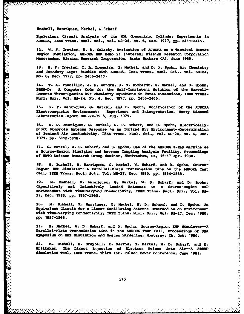
,7-77
Bushell, Manriquez, Merkel, & Scharf
Equivalent Circuit Analysis of the HDL Concentric Cylinder Experiments inAURORh, IEEE Trans. Nucl. Sci., Vol. N8-24, No. 6, Dec. 1977, pp. 2411-2415.
12. W. F. Crevier, X. D. Kalasky, Evaluation of AURORA as a Tactical SourceRegion Simlation, AURORA ZNW Memo 21 (internal Mission Research CorporationMemorandum, Mission Research Corporation, Santa Barbara CA), June 1980.
13. W. F. Crevier, C. L. Longmire, G. Merkel, and D. J. Spohn, Air Chemistryand oundary Layer Studies with AURORA, IEEE Trans. Nucl. Sci., Vol. 8-24,No. 6, Dec. 1977, pp. 2406-2410.
14. T. A. Tmmolillo, J. P. Wondra, J. N. Bombardt, G. Markel, and D. Spohn,PRES-D: A Computer Code for the Self-Consistent Solution of the Maxwell-Lorentz Three-Species Air-Chemistry Equations in 2hree Dimensions, IEEE Trans.Nul. Sci., Vol. N8-24, No. 6, Dec. 1977, pp. 2456-2460.
" 15. R. P. Manriquez, G. Merkel, and D. Spohn, Modification of the AURORA• Electromagnetic Environment: Experiment and Interpretation, Harry Diamond
Laboratories Report HDL-PR-79-5, Aug. 1979.
16. R. P. Manriquez, G. Merkel, W. D. Scharf, and D. Spohn, Electrica-lly-Short Monopole Antenna Response in an Ionized Air Environment--Determinationof Ionized Air Conductivity, IEEE Trans. Nucl. Sci., Vol. N5-24, No. 6, Dec.1979, pp. 5012-5018.
17. G. Merkel, W. D. Scharf, and D. Spohn, Use of the AURORA X-Ray Machine asa Source-Region simulator and Antenna Coupling Analysis Facility, Proceedingsof NATO Defense Research Group Seminar, Shrivenham, UK, 15-17 Apr. 1980.
18. M. Bushell, R. Manriquez, G. Merkel, W. Scharf, and D. Spohn, Source-Region EMP Simulator--A Parallel-Plate Transmission Line in the AURORA TestCell, IEEE Trans. Nucl. Sci., Vol. N8-27, Dec. 1980, pp. 1834-1838.
19. N. Bashell, R. Manriques, G. Merkel, W. D. Scharf, and D. Spohn,Capacitively and Inductively Loaded Antennas in a Source-Region MIPEnvironment with Time-Varying Conductivity, IEEE Trans. Nudl. Sci., Vol. NB-27, Dec. 1980, pp. 1857-1863.
20. M. Bushell, R. Manriquez, G. Merkel, W. D. Scharf, and D. Spohn, An" Equivalent Circuit for a Linear Oscillating Antenna Immersed in an Environment
with Time-Varying Conductivity, IEEE Trans. Nucl. Sci., Vol. NS-27, Dec. 1980,pp. 1857-1863.
21. G. Merkel, W. D. Scharf, and D. Spohn, Source-Region EIP Simulator--AParallel-Plate Transmission Line in the AURORA Test Call, Proceedings of DNASymposim on DIP Simlation and System Hardening, Monterey, CA, Oct. 1980.
22. M. Bashell, S. Graybill, K. Kernt., G. Merkel, W. D. Scharf, and D.Whittaker, The Direct Injection of Electron Pulses into Air--A BREWSimuilation Tool, IEXE Trans.* Third Into Pulsed Power Conference, June 1981.
1701i: 70 -r:
.4
I 4:"
, - .. ,- .- = .. ,. .. , - - . , -'-'-' . :-. " - -*", *.--. "- .-"
. -"
Bushell, Manriquez, Merkel, Scharf
23. N. Rshell, R. Hanriquez, G. Merkel, and W. D. Scharf, Simulated DeepSource-Region EMP Coupling to Cylindrical Objects, IEEE Trans. Nuclo Sci.,Vol. 35-28, No. 6, Dec. 1981, p. 4457.
24. M. Bashell, R. Manriquez, G. Merkel, W. D. Scharf, Measurement andCalculation of the Short-Circuit 8lIMP Response of Vertical OscillatingHelical Antennas and Oscillating Loop Antennas, IEEE Trans. Ncl Sci., Vol.V5-28, No. 6, Dec. 1981, p. 4495.
25. L. Ambrose, M. Bushell, C. Ksnyon, G. Merkel, W. D. Scharf, microwaveMeasurements of Conductivity in Air and Other Gases, IEEE Trans. *1ucl. Sci.,Vol. 35-28, No* 6, Dec. 1981, p. 4426.
26. M. Bushell, R. Gray, C. Kenyon, R. Nanriquez, G. Merkel, and W. D.Scharf, Strategic and Tactical Source-Region IP Simulation Techniques, DNAConf. on Instrumentation for Nucl. Weapons Effects, March, 1982.
' 27. G. Merkel, W. D. Scharf, and D. Spohn, Simulation of Large CouplingStructures in a Source-Region ZMP Environment, DNA Symposium on IMP Simulationand System Hardening, Monterey, CA, Oct. 1980.
28. H. J. Longley and C. L. Longmire, Development and Testing of LEMPI, LosAlamos Scientific Laboratory LA-4346, April 1970.
29. H. A. Sandmeir, S. A. Dupree, C. Z. Hanson, Electromagnetic Pulse andTime-Dependent Escape of Neutrons and Gamma Rays from a Nuclear Explosion,Nucl. Sci. and Eg., Vol. 48, 1972, pp. 343-352.
30 . G. Merkel and W. D. Scharf, "Source-Region Electromagnetic PulseSimulator", U. S. Patent Application #252737.
31. A. G. Stewart, "CAMELOT--A Novel Concept for a ultiterrawatt Pulse PowerGenerator for Single Pulse, Burst or Repetition Rate Operation", Harry DiamondLaboratories Report HDL-SR-81-1, April 1981.
171
4
° . . .... V .~~.-
CAMPBELL
CONTROL OF PARASITIC CURRENTS ONRADIATING SYSTEMS
DONN V. CAMPBELL, PH.D.US ARMY COMMUNICATIONS-ELECTRONICS COMMAND
FORT MONHOUTH, NEW JERSEY 07703
I. INTRODUCTION:
Military communication antennas operating in the 2-30 Mlz high fre-quency (HF) band, 30-90 MHz very high frequency (VHF) band, and the 200-400 MHz ultra high frequency (UHF) band are installed on vehicular, ship-borne, airborne, manpack, or fixed platform. Short, medium and longrange radio is supported by HF, Net Radio is serviced by VHF, and ground-to-air communication employs UHF. The antenna engineer is confronted withthe task of designing small efficient radiating system having wide band-width and predictable impedance and radiation characteristics. In thepast, wide bandwidth has been achieved at HF and VHF by band switching andbroadband matching circuits. However, new requirements for wide Instan-taneous bandwidth (no tuning) antennas have been Imposed with the adventof frequency hopping radios.
Antenna interaction (mutual coupling) and electromagnetic compatibility(EMC) are major concerns when many antennas and communication systems arecollocated in a confined area, as in a command post or an air traffic con-trol facility. System performance may be unpredictable due to antennamutual coupling effects. The purpose of this paper is to demonstrate, bycomputer analysis, and validating experimental measurements, that extran-eous parasitic radio frequency (rf) currents on radiating systems can
*. impair performance, causing field pattern distortion, crosstalk interfer-ence, and unpredictable behavior with changes in operating frequency.
*. . It is shown that parasitic currents can be suppressed in both narrowband* . and wideband radiating systems. The techniques discussed are practical
and are applicable to field use where accepted procedures for antennainstallation are sometimes set aside because of lack of understanding,or for expediency.
This paper is organized as follows: the horizontal dipole aboveground is studied, and it is shown that parasitic currents on the sheathof the coaxial feed line can be suppressed. Similarly, the inverted-V
175
,',,:. -,. ................ ... .... .... ... ..... ...
dipole is shown to have significant parasitic feed lfne currents vhic.can also be eliminated. Extraneous rf currents on the met supporting avertical dipole are shown to be substantially reduced over a narrow fre-quency range by the addition of a quarter-vave detuning stub and over amuch wider frequency range by means of a broadband cable choke. Associatedradiation patterns confirm the improvement obtained when parasitic currentsare suppressed. A broadband colnear dual antenna providing more then 35decibels (dX) of inter-dipole isolation is described. The high isolationresults from the collnear antenna arrangement, and by virtue of the specialfeed line "Isolator Section" which acts as a band elimination filter forthe parasitic currents induced on the feed line of the upper dipole. Thisantenna system allow duplex operation free from crosstalk interferenceIn an air traffic control facility.
II. PARASITIC CURRENTS ON HORIZONTAL DIPOLES
The horizontal dipole center fed by coaxial line is extensively used.It is known that tmequal electromgetic forces on each half of thisantenna cause a condition of lmblance which may resultin unequal currentsin the antenna arm. The feed line coupled to the antenna may supportparasitic currents of appreciable magnitude. In an earlier experimentalstudy, the currents on a horizontal dipole above ground were measured (1).This earlier study demonstrated conclusively, that significant currentImbalance may occur. It also showed that current balance in the antennaarms could be Improved by simply connecting a cable choke between the di-pole and the feed lne. In essence, the cable choke acts as an effectivehigh Impedance circuit which nterrupts the rf current flowing on theouter surface of the feed line.
For comparison purposes, the experimental horizontal dipole was modeledon the Numerical Electromagnetic Code (NEC), a computer program foranalysing the electromagnetic response of antennas (2). The antenna isshown in Fig. 1. To facilitate measurements of current distribution, theexperimental dipole was Installed seven feet above the ground, and it wasmodeled on the computer accordingly. In the computer model perfectly con-ducting ground was assumed and the bottom of the feed line was assumed tobe connected to the ground.
Although the length of the modeled antenna is a half wavelength at 4s, such an antenna might be operated in the field at other frequencies
without bothering to adjust its length to resonance. To investigate thispossibility, the current amplitude distribution at 2 Nuz was determined,md is shown in 1ig. 1 by the dashed line curve. The experimental andcomputed distributions are similar. It Is sen that the current imbalanceis pronounced and that the feed line supports a parasitic current ofappreciable amplitude on its outer surface.
176
W ," ... ;," , ", . ." - " . .'. *" . .,, .''"""'''''" , .- ' ". ' ' -" '-""" "" ""....
CAMPBELL
As stated earlier, a cable choke was used to suppress parasitic currenton the feed line and to improve current balance on the arms of the experi-mental dipole antenna. A cable choke consists of coaxial cable shaped intoa helical coil, as shown in Fig. 2(a), or in the form of a toroid. In theexperimental study, the cable choke consisted of thin coaxial cable woundon several high permeability ferrite toroids. Regardless of the construc-tion, however, the cable choke impedance between points A and B at theouter surface of the transmission line (see Fig. 2(a)) is essentiallyequivalent to a high Impedance circuit consisting of an inductance L con-nected in parallel with capacitance C, as shown in Fig. 2(b). When lossesare neglected, the reactance of the choke is, to good approximation, given
-* by X - 27rfL/ (I - (f/fo)e) where the self resonance frequency is fo-1/21r 7U. In practice, cable choke losses will be present and should beminimized.A
In wide bandwidth applications, it is practical to design the cablechoke so that it resonates at the geometric mean frequency fo - VTLfa fuwhere f a and fu denote, respectively, the lower and upper frequency limits.When so designed, the reactances at the frequency limits will be equalin magnitude. The bandwidth of the cable choke is inversely proportionalto the self capacitance. Thus, to maximize the isolation bandwidth, thecable choke should be designed for maximum inductance and minimum capaci-tance.
When the cable choke was connected between the dipole and the feedline, in the manner shown in Fig. 3, it was found that the parasitic cur-rent on the feed line was essentially eliminated, and the antenna currentbalance was improved. The impedance of the cable choke used with theexperimental diple antenna was (3120 +- J4550) ohms at 2 MHz (1). Theeffect of this choke was accounted for in the NEC computer model byinserting this impedance between one arm of the dipole and the feed line.It is seen that the calculated and measured currents are comparable.Although not shown here, similar improvements in the current distributionare effected at 4, 6, and 8 MHz, demonstrating that the cable choke pro-vides an effective means of suppressing parasitic currents over a broadfrequency range.
III. PARASITIC CURRENTS ON INVERTED-V DIPOLES
The inverted-V dipole with drooping arms is an easily erected antennarequiring only one support at its midpoint. As in the previous example,the NEC computer program was used to obtain the current distributions withthe feed line connected directly to the antenna and with a cable choke
V interposed. The inverted-V shown in Fig. 4 is resonant at approximately7 MHz. At resonance, currents in the antenna arms arc well balanced andthe feed line excitation Is minimal. However, if the antenna is operated
17
177
............................. "..
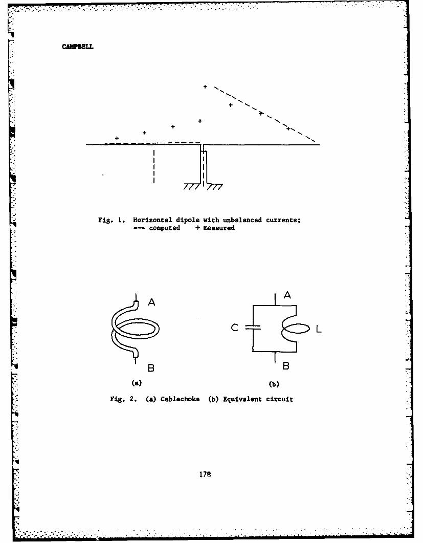
CAMPBELL
+N+N
777177
Fig 1.Horzonal ipoe wth nlnecurts
-- coptd +maue
A
/A
(a) (b)
Fig. 2. (a) Cablechoke (b) Equivalent circuit
1 78
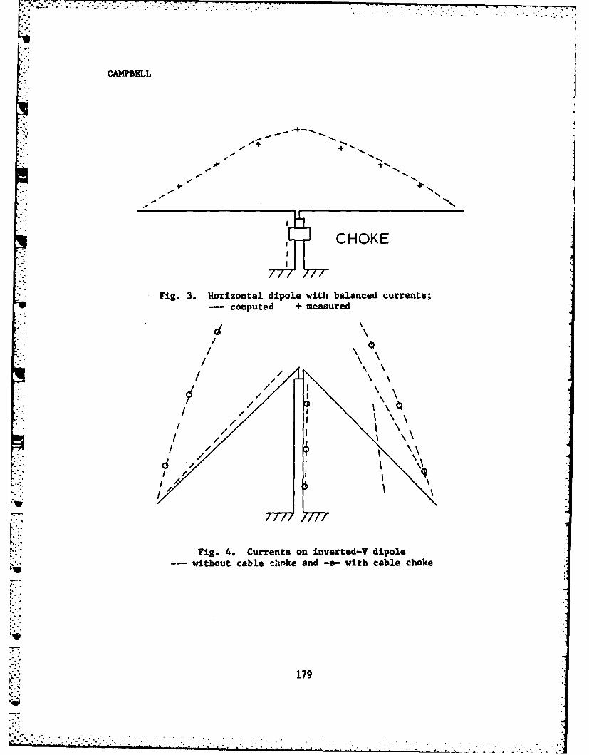
CA14PBELL
- --- s. +
-CHOK
Fig.3. oriznta diple ith alaced urrnts
-copte eaue
A5
777 71~
Fig 4.CretNninet Vdpl
Fi-- 3.thoritonale dipole aith balanced curents;k
coptele esue
17
*'CAMPBELL
at frequencies above or below resonance, current imbalance and feed lineexcitation will increase. The current amplitude distribution obtained at4 MHz, for example, confirms this expectation. See Fig. 4. Note that inthis computer model, the lower end of the feed line is assumed to be con-nected to perfectly conducting ground.
The inverted-V dipole with a cable choke connected in series with thefeed line was also investigated. The impedance of the cable choke at 4MHz is assumed to be (3935 + J2937) ohms. The lower end of the feed linein the model does not contact the ground, simulating an ungrounded instal-lation. In the computer model "average" ground having a relative permit-tivity of 15 and conductivity of .005 mhos per meter was assumed. It is
* seen in Fig. 4 that the cable choke eliminates parasitic current on thesheath of the feed line and balances current in the antenna arms. It isinteresting to note that the inverted-V feed-point impedance is (30.1 -J857) ohms with the cable chike present and is (542 + J1942) ohms withoutthe cable choke. This change in impedance is attributed to the markedlydifferent current distributions obtained for the two cases. If a metalsupport mast is used, an insulator should be provided at its top to prevent
* "short-circuiting" the cable choke.
IV. PARASITIC CURRENTS ON MAST-MOUNTED DIPOLES
Mast-mounted vertical dipoles are extensively used at VHF and at UHF.The dipole can be electrically decoupled from its support by attaching aquarter-wavelength detuning stub to the mast, or to the feed line asshown in Fig. 5(a). Provided that the stub is properly dimensioned, itintroduces a high impedance at the lower end of the dipole cutting offthe line current or mast current below. The current amplitude on theresonant stub is maximum at the shorted end. The section of feed line ormast adjacent to the stub carries both the antenna current and the trans-
* mission line current. The transmission line currents are in oppositedirections in the stub and adjacent mast so that the resultant current issmall. Other applications of stubs appear in the literature (3, 4).
If the length of the stub is somewhat different from a quarter-wave-length at the operating frequency, it is then ineffective because its im-pedance is too low to enforce a current minimum on the mast. This is
S illustrated in Fig. 5(b), where the non-resonant stub has little effect.Evidently, detuning stubs are effective but in narrowband applications.
When the mast currents are suppressed, as in Fig. 5(a), it is foundthat the field strength on the horizqn increases. Conversely, the fieldstrength on the horizon is reduced when parasitic current is not sippressed.The vertical radiation patterns for these two cases are shown in Fig. 6.For the assumed conditions, the power gain on the horizon is increased bymore than 6 dB by suppressing the mast currents. This, of course, trans-
180
U-
AD-Ri20 811 PROCEEDINGS OF THE ±982 ARMY SCIENCE CONFERENCE HELD AT 3/6THE UNITED STATES.. (U) DEPUTY CHIEF OF STAFF FORRESEARCH DEVELOPMENT AND ACOUISITIO. is JUN 82
UNCLASSIFIED F/G 5/2 N
monEEEEEmmuiEEhElgmhllhhhEDEEE**DiEiEEiEFIIIEIhIIEIIIEII10100l3101011uuuununnugunnuEosmEmmmoEE-
-I
MIRCP RSUTCNTS HRTMRC~IOf~LTS HR
URM 1SAIOIS160
MIMICOCOOY RESOUTIO TEST. CHART
N-O WNW OFW IWUJ 0 PAGOADS1H3A - ---
~" I
.16 M. Ii~~
- ~ ~ ~ IRCP mownM TEW CHARTPYSo~T~-U.AW SMEMI OF SVMIU-3963.
L I. -O u
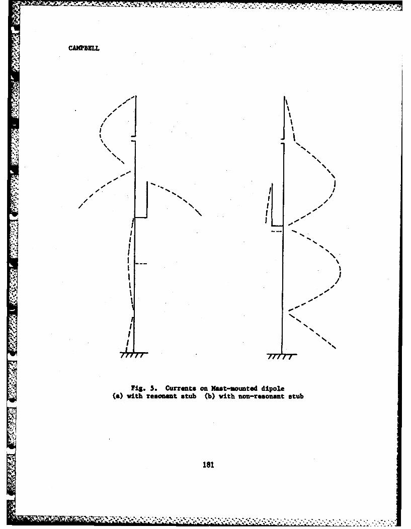
a a N . *...>.~. *
CAlf DELL
ii.-'a. -
-- I
/- I/
'a
/ Ii -% / ~I1 '4..4..
'4
I "a
I. 'a
S I ,1
1I
I 4.4I .4.4..
I 4%I 'a' "a4.4
Fig. 5. Currents on Mast-mounted dipole(a) with resonant stub (b) with non-resonant stub
S -~
lel
~ .%~.*.* *.. ..- 'a......
.* .. - a a * . , . . -
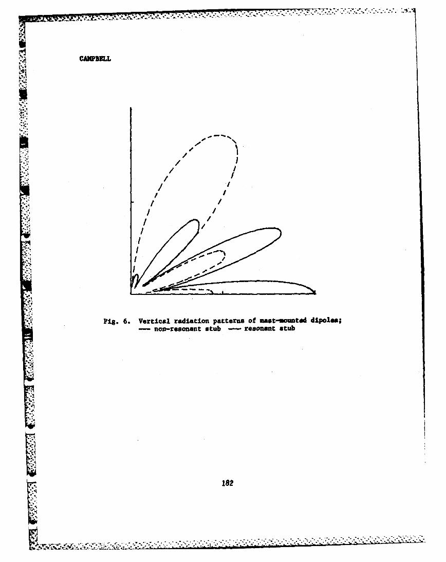
*1182
CAMPBELL
lates into greater operating range.
The dipole can also be decoupled from the mast and from the feed lineby a cable choke as shown in Fig. 7. To test this hypothesis, a URF dipolewas modeled, using NEC, and the current distribution at 300 MHz determined.The cable choke was assumed to be equivalent to a parallel LC circuit (seeFigs. 2(a) and 2(b)) with constants appropriate to UHF. The current isessentially confined to the half wavelength dipole and is relatively weakon the mast or feed line. Even better results could be obtained if thecable choke were resonant at the operating frequency. In this examplethe LC constants chosen cause the choke to resonate at 258 Mlez, which issomewhat lower than the operating frequency. The radiation pattern wouldbe siuilar to that already shown (Fig. 6) for the antenna with resonantdetuuing stub.
V. PARASITIC CURRENTS ON A COLINFAR DUAL ANTENNA SYSTNf
In duplex communication systems, the mutual coupling of the collocatedtransmitting and receiving antennas can result in crosstalk interference.It is well known that radiation coupling between two dipole antennas ismuiniized when they are mounted colinearly, and sufficiently spaced. Asecond coupling effect, due to parasitic currents Induced on the feed lineof the upper dipole, is more difficult to control than radiation coupling.With radiation coupling minimised, this second coupling effect predominates.
It has been demonstrated recently that these parasitic currents can besuppressed over an octave frequency range by means of an "isolator section"incorporated n the feed line of the upper antenna (5). The feed lineisolator section consists of a sequence of high impedance cable chokesplaced in the coaxial line at quarter-wavelength intervals. It behaveselectrically as a band elimination filter which reduces the interantennacoupling caused by currents on the transmission line sheath.
The colinear dual antenna is shown in Fig. 8. The isolator section inthis antenna has five cable chokes. The antennas are independently feddipoles. A computer model of this antenna yields the current distributionshown when the upper dipole is excited, and the lower dipole is terminatedin 50 ohms. It is seen that current is essentially restricted 'e drivendipole, and is very weak along the rest of the antenna system. so-lation between the upper and lover dipole is defined as the frac thetotal power radiated by one dipole which is intercepted by the ot4er dipole.The nterdipole isolation of the antenna system (Fig. 8) was found to be atleaut 35 dD from 200 to 400 Wsll, indicating that radiation coupling is thelimiting factor for the given antenna spacing.
183
'\ :* V7,
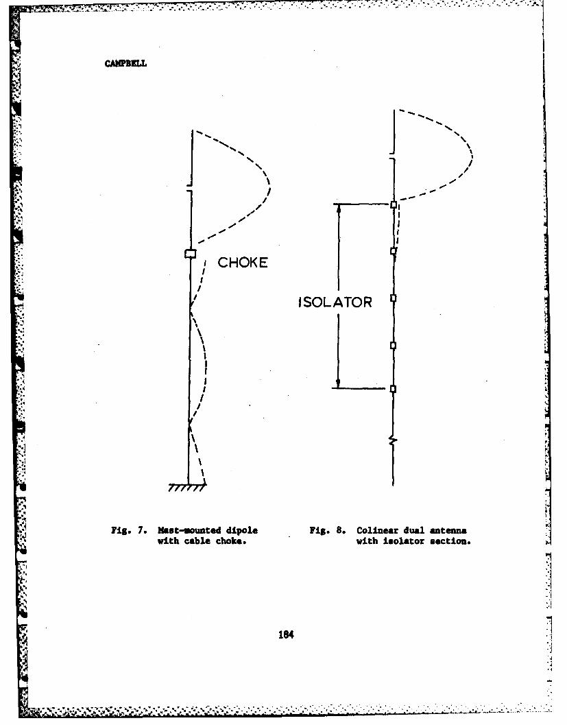
-F CAMPBELL
14
'2 / CHOKE
ISOLATOR
Pi@7 at-utd ioeFS .Clierda nen
wih abe hoewthislaorsetin
I 84

7 17
CAMPBELL
VI. CONCLUSIONS
In this paper, it has been clearly shown that induced parasitic rfcurrents can seriously degrade the performance of a radiating system; yetthe significance of these undesired spurious currents has been largelyignored by antenna designers, and field users alike. It has been shownthat parasitic currents can be effectively suppressed in both narrowbandand wideband antenna systems by means of quarter-wavelength stubs(resonance method) and broadband cable chokes. Although effective currentsuppression techniques exist, further study is necessary to establishengineering design criteria and to extend state-of-the-art current suppres-sion techniques to multi-octave antenna systems.
REFERENCES:
,::: (1) J. P. Muro, "Investigation of Unbalanced and Force BalancedDipole Antennas," Master's Project, Newark College of Engineering, Newark,NJ, 1968.
(2) J. G. Burke, A. J. Poggio, J. C. Logan, and J. W. Rockway, "NEC-Numerical Electromagnetics Code for Antennas and Scattering," in IEEE 1979Int. Symp. on Antennas and Propagat., Vol. 1, pp. 147-150, Seattle, WA.
(3) R. W. P. King, H. R. Himno, and A. H. Wing, TRANSMISSION LINES,N ANTENNAS AND WAVE GUIDES, New York, Dover Publications, Inc., 1965.
(4) J. S. Belrose, "On Minimizing the Effects of Re-Radiation fromPowr Transmission Lines on the Radiation Pattern of MF-AM BroadcastingAntenna Arrays," lEE Second Int. Conf. on Antennas and Propagat., Part 1,pp. 33-37, York, U.K., 1981.
(5) D. V. Campbell, S. Fich, and F. K. Schwering, "Suppression ofParasitic Currents on Feed Lines of Colinear Dual Antenna Systems," IEEETrans. Antennas Propagat., Vol. AP-28, pp. 658-662, Sept. 1980.
i
CAMPI
DESIGN OF MICROSTRIP LINEAR ARRAY ANTENNASBY COMPUTER
MORRIS CAMPI, PH.D.U*S. ARMY ELECTRONICS RESEARCH AND DEVELOPMENT COMMAND
HARRY DIAMOND LABORATORIESADELPHI, MARYLAND 20783
Introduction
Research in microstrip antenna technology and design is currentlybeing developed to meet the present and future needs of military radar andfuze system requirements. Configured in either single- or multiple-lattice structures, microstrip has the advantages of ease in fabrication,low cost, light weight, and structural conformability. When designed tohave either a series or a corporate feed network, the lattices becomeantenna arrays that can be used for transmitting and receiving signalsfrom microwave through millimeter frequencies into the lower regions ofthe near-millimeter wave portion of the spectrum. However, the presentstate of the art is at the same stage of development as existed forwaveguide slot array designs in the late 1950's and early 1960'8. Thisstage is a *cut-and-try" period in which an empirical design takes fromweeks to months of fabrication and testing before satisfactory results areobtained, even then, one can never be sure of achieving the optimum designto meet the system's specific requirements.
Today, computer aided design codes can be developed to help antennaengineers in their design of linear or planar array microstrip antennas.This report describes one such code that was developed by using bothempirical data and a theoretical model. One major feature of this code isthat it allows the designer to vary any one or more of the antenna design
*parameters and to observe the results, such as changes in the radiationpattern or amplitude distribution displayed at the computer terminal
* screen. This application provides the tool required by the engineer todetermine in a matter of seconds the prime factors affecting his designand to make parametric adjustments or sensitivity studies to helpunderstand and develop his final product. Once a design is established,the engineer is presented with a set of coordinate numbers that can beplaced on magnetic or paper tape, which can then be used to fabricate theantenna on printed circuit board without the need for drawings or art-'
187
* 4
.4i ' - , , - ,,-, ., " , , , .. -. . ,., ,,.. . ,. - . .. . ...
'-.,
CAMPI
layout work and thus simplify the engineering process and reduce the time
spent.
The computer program reported will continuously evolve. As better
data or refinements in the analytical models are produced, they will beincorporated into the program.
Microstrip Linear Array Antenna
.icrostrip arrays, like other array designs, have a power feed'- arrangement that is classified as being either series or corporate feed.
A series-feed array is designed so that each element connects with thenext element in series with the input power or receiver being applied atone end of the array. In a corporate-feed array, each element isindependent of each other, and a prescribed level of power is individuallytransferred to or received from each element by separate means or by useof a power divider network. The radiation characteristics of either typeof antenna are essentially those produced by the electromagnetic fieldsthat illuminate the antenna aperture. (The far-field radiation pattern isrelated to the Fburier transform of the aperture illumination.) Aconstant amplitude of illumination at each array element produces asin2 x/x 2 -like pattern in the far field with 13.2-dB side lobes below themain beam. Other distributions produce far-field patterns with otherlevels of gains, beam widths, and side lobes, each dictated by the antennaaperture distributions. Over the years, some specific distributions havebeen introduced and used by engineers to satisfy their systemsrequirements. These distributions have since become quite common in theindustry.
Control of the aperture distribution in a corporate-feed array isfairly simple. However, the feed or power dividing network itself canbecome complicated and, if designed in microstrip, radiates and causes adistortion in the radiated power distribution. A series-feed array,however, has no independent feed network, but is power fed from one end.As the power traverses along the array, some power radiates from the firstelement and the rest continues until all the elements radiate theremaining power. The aperture distribution in this case is determined bythe radiation characteristics of each element and their relation to all ofthe other element characteristics. A computer analysis of this type ofarray can be obtained once the single-element characteristics along withthe array neighbor-to-neighbor interactions are understood.
Single Element Patch Model
The geometry of the single element microstrip patch is shown infigure 1. It consists of a thin rectangular conducting plate positioned
~18
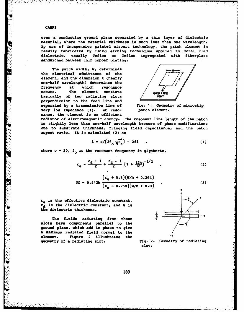
CAMPI
' over a conductinq ground plane separated by a thin layer of dielectricmaterial, where the material thickness is much less than one wavelength.By use of inexpensive printed circuit technology, the patch element isreadily fabricated by using etching techniques applied to metal claddielectric, usually Teflon or Teflon impregnated with fiberglasssandwiched between thin copper plating.
The patch width, W, determinesthe electrical admittance of theelement, and the dimension A (nearlyone-half wavelength) determines thefrequency at which resonanceoccurs. The element consistsbasically of two radiating slots Z Z/perpendicular to the feed line andseparated by a transmission line of Fig. 1. Geometry of microstipvery low inVedance (1). At reso- patch element.nance, the element is an efficient
- radiator of electromagnetic energy. The resonant line length of the patchis slightly less than one-half wavelength because of phase modificationsdue to substrate thickness, fringing field capacitance, and the patchaspect ratio. 'It is calculated (2) as
t- c/(2f° E) - 26t , 1)
where c = 30, fo is the resonant frequency in gigahertz,
=.-i--+ ~ -2 +d j /2e C (2)
(Ce + o.3)(W/h + 0.264)61 0.412h (3)s)(/ os
(Ce .5)Wh+08
e is the effective dielectric constant,* Cd is the dielectric constant, and h is
the dielectric thickness.
The fields radiating from these T* - slots have components parallel to the
ground plane, which add in phase to givea maximum radiated field normal to the
Uelement. Figure 2 illustrates thegeometry of a radiating slot. Fig. 2. Geometry of radiating
slot.
189
....-. ..... -
7;, 7. 77 777-7-7 'l
CAMPI
The total power radiated from each slot is obtained by integratingthe real part of the Poynting vector from a single slot over a hemiiphereof large radius. It is derived as
2 fw sin2 (W sin *.4 VOI XO
P = -Cos' do , (4)0 sin 2 o
where V0 is the voltage across the slot of height h, which is very small,that is, k0h << 1, where k is the propagation constant equal to 2w/A0.
Microstrip Element Conductance
Since rigorous transmission line or two-port parameters are notavailable for a resonant, radiating microstrip patch, it is modelled as alumped conductance and a phase delay. The delay is taken into account for
.. the phasing of series-feed arrays; the combined power radiated by the twoslots of a patch is the same as that dissipated by the conductance, G,having across it the voltage, V0 , at the center of the slot; hence, GP/V2 or G = I/w/j, where
0
.. sin 2 (LW sin *)-.:' cos3 do • (5)
-: sin 2
The integral, I, is solved by use of computer integration techniques. Inthe range 0.033 < W/X0 < 0.254, conductance values have been measured andfollow the relation (3)
G= 0.0162 (!L)1.757 (6)
Insertion Phase
Transmission line discontinuities produce phase shifts or delays inthe propagation of energy down the transmission line. The impedancemismatch and line-to-patch width aspect ratio at the entrance and exitports of each microstip patch produce phase delays to the propagatingsignal. Most importantly, mode structure and wave number along thelongitudinal axis of the microstrip cavity can introduce a large insertionphase shift between input and output ports in addition to the desiredphase shift of 1800. This effect does not alter the resonance conditionof the patch, but increases the effective phase delay to the followingpatch in the array and thus changes the composite radiation pattern. Fbrexample, if all the patch widths were equal, the resulting constantinsertion phase of each patch would rotate the main lobe of the antennapattern. However, most array designs require element widths of different
190
*-,' .14 .- ,'; ,- ,-,,,,,. 4 .. . .. . .. . . ..... . .. ............-......-.-...-. -..- . .,.- .. --... ', :.:- : ,: :..........
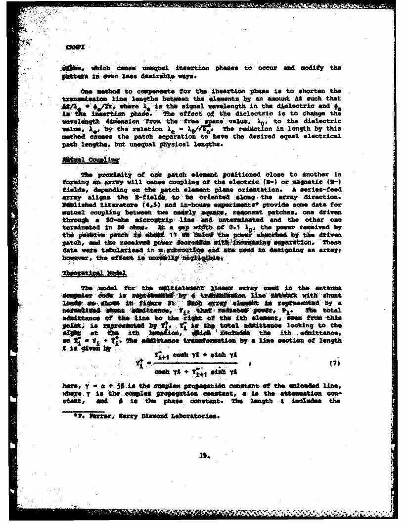
as, i 0UL6S 0 c Aue unefl Insertion phases to occur and modify thepittam in evn les desirable ways.
One method to compensate for th insertion phase is to shorten thet~lUmlsSOi line lengths between the elements by an amount At such that
* f ~li*4 $/ *hitre IC is the signal wavelength in the dAlectric and'i*te insertion pha .' te effect of the dielectric is to change thewsnlelgth d11mesion' Io the'ftes p.ce vain , A0, to the dielectricvalue, f -by the relation X X , The redttion in length by thismethod causes the patch separation to have the desired equal electricalpath l ngths, but unequal physical lengths.
The proximity of oni patch element positioned close to another inforing s array will caus coupling of the electric (R-) or magnetic (R-)fields, depending c .the patch element plane orientation. A series-feedarray al igns, the W-fiete1*. to -be oriented along ithe array direction.Pihlshed literatue (4S) anid in-house eperlmentr provide some data formutual coupling between two nearly rre, o r t patches, one driventtrov a 5-ohl sicrostrip -line and usttiaated and the other onetesmstsed in S afm. A* gap ti .of 0.1 X, the power received bythe , #o4* ptdt 1- SW0 170 '67 l516 the power abeokMfd bf* the. drivenpatch, and the remiW& p r ao44S* *itj4 iinepVarion, Thesdata vweft tabularised in Afesbrovttue and ae sed in designing an array#how*vr, theeff*c ii Aotd"flp "
he model for the mftilent Uiea array used In the antenna
lZe, a toef iom fSA n R lb kE. itrq el4M e$aet! by Anested' mit -4fttaoV At, tba inSutmf "Poft, P. ISe totaladittane e of te in to the right of the ith lo n,# as fkti thispaife is fpr*Atts i 4. 7 ' tthe .tta aftitt a e looking to the
911e ai eti, & swans. theIth .d aittance,st1*11 + 1 h 4 tt a tt, by aline section of length
Vj a yA + sink yt4(7)
hre, ya *+ is. the omplexprop constant or the un ded line,where y is tler espies Popagatiost co0nstat, a is the atutoncorn-stanii, at is ,the pha6e constant. The length it includes the
'V. kfrr, Barry Diamond Laboratories.
ta
X3 N-Fe
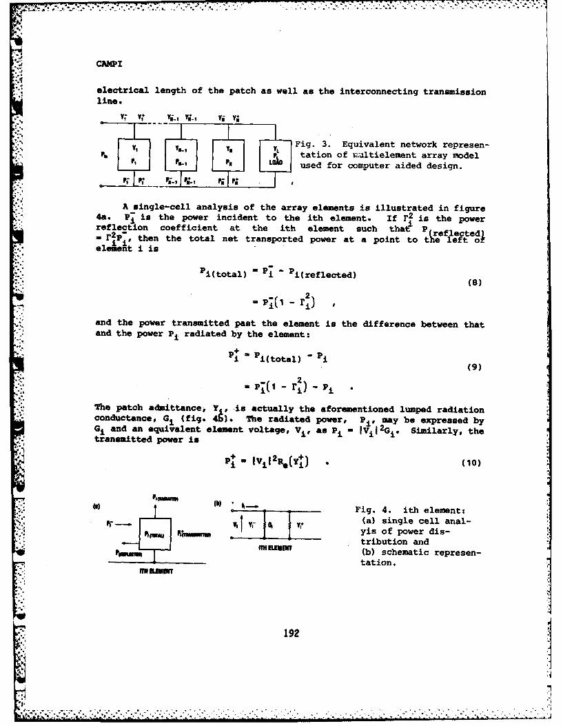
-. . + ' '+. + . - ' .+ . " "- - . ."• + . - - . . + . . . . . . . - - - - - + - - + -
CAMPI
I
electrical length of the patch as well as the interconnecting transmissionline.
Y; YI* Yi_, vI .Y I Vi Y+
YN V, Fig. 3. Equivalent network represen--. I U LDp tation of r,.utielement array model
P LOA used for computer aided design.
A single-cell analysis of the array elements is illustrated in figure4a. PI is the power incident to the ith element. If r2 is the power
±reflection coefficient at the ith element such that Pr:2 -(reflected)Pi, then the total net transported power at a point to the left ofii
element i is
Pi(total) Pi - Pi(reflected)(8)
and the power transmitted past the element is the difference between thatand the power Pi radiated by the element:
S= Pi(total) - Pi
(9)I .": -,(i -r[ "i
The patch admittance, Y , is actually the aforementioned lumped radiationconductance, Gi (fig. 45). The radiated power, Pi, may be expressed byGi and an equivalent element voltage, V., as Pi - Ivil %i. Similarly, thetransmitted power is
P,- IVil2R.(Yt) • (10)
() Mb Fig. 4. ith element:" --L "z (a) single cell anal-
Ir5m yis of power dis-tribution and(b) schematic represen-tation.
192
j 2
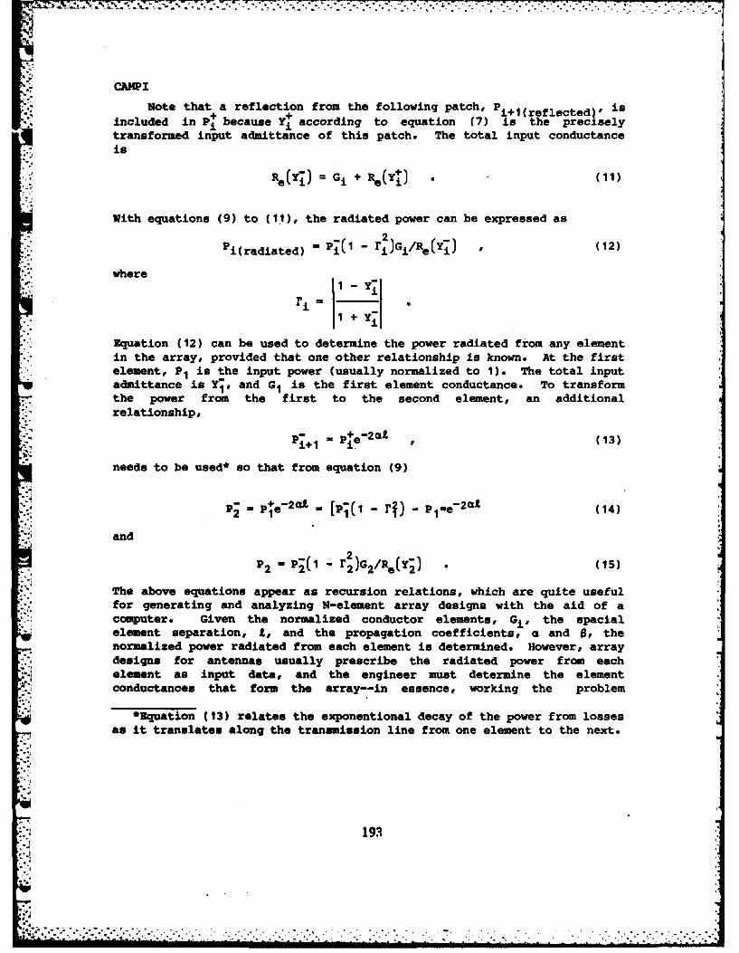
CA3PI
Note that a reflection from the following patch, Pi+llreflected • isincluded in Pi because Yj according to equation (7) is the preciselytransformed input admittance of this patch. The total input conductanceis
Re(Y7) = Gi + ReCY) . (11)
With equations (9) to (11), the radiated power can be expressed as
Pi(radiated) '= - ri)Gi/Re(Yi) , (12)
whereI - Y1
1 +
Equation (12) can be used to determine the power radiated from any elementin the array, provided that one other relationship is known. At the firstelement, PI is the input power (usually normalized to 1). The total inputadmittance is Y¥, and G1 is the first element conductance. To transformthe power from the first to the second element, an additionalrelationship,
P+I Pie 2 a (13)
needs to be used* so that from equation (9)
'-: =p+e-2" = [P-C1 r2 p -e-20 ( )2 e ~ 1 *Q (14)
and
p2 2 -2)G 2/Re(r2) (15)
The above equations appear as recursion relations, which are quite usefulfor generating and analyzing N-element array designs with the aid of acomputer. Given the normalized conductor elements, Gi, the spacialelement separation, t, and the propagation coefficients, a and 0, thenormalized power radiated from each element is determined. However, arraydesigns for antennas usually prescribe the radiated power from eachelement as input data, and the engineer must determine the elementconductances that form the array--in essence, working the problem
*Equation (13) relates the exponentional decay of the power from lossesas it translates along the transmission line from one element to the next.
Z.'
193
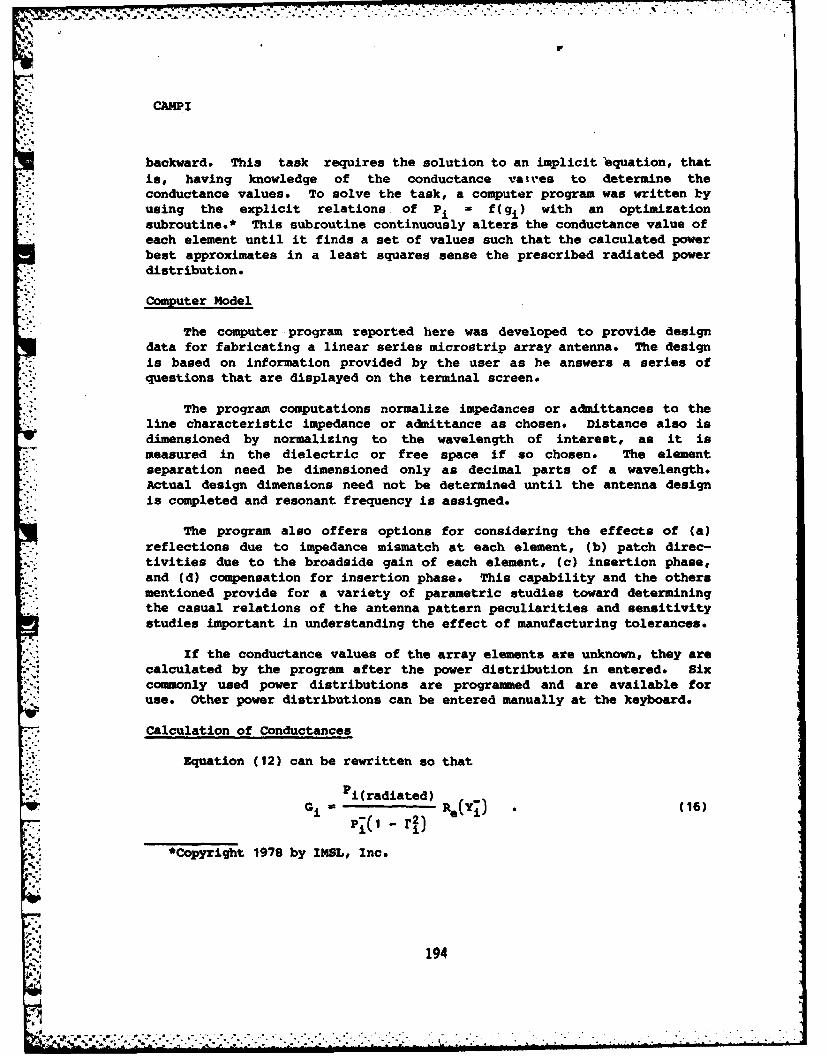
* .X t.!J a.. + ,,- , - , -, , + ,, -. -+ ", -" . '' - ._ -_'. - - .' .' - . ' • . +. . . + - "- - - "- - • . - - .-
CAMPI
backward. This task requires the solution to an implicit 'equation, thatis, having knowledge of the conductance vait'es to determine the
conductance values. To solve the task, a computer program was written byusing the explicit relations of P = f(gi) with an optimization
* .. subroutine.* This subroutine continuously alters the conductance value ofeach element until it finds a set of values such that the calculated power
best approximates in a least squares sense the prescribed radiated powerdistribution.
Computer Model
The computer program reported here was developed to provide designdata for fabricating a linear series microstrip array antenna. The designis based on information provided by the user as he answers a series ofquestions that are displayed on the terminal screen.
The program computations normalize impedances or admittances to theline characteristic impedance or admittance as chosen. Distance also isdimensioned by normalizing to the wavelength of interest, as it ismeasured in the dielectric or free space if so chosen. The elementseparation need be dimensioned only as decimal parts of a wavelength.Actual design dimensions need not be determined until the antenna designis completed and resonant frequency is assigned.
The program also offers options for considering the effects of (a)reflections due to impedance mismatch at each element, (b) patch direc-tivities due to the broadside gain of each element, (c) insertion phase,and (d) compensation for insertion phase. This capability and the othersmentioned provide for a variety of parametric studies toward determiningthe casual relations of the antenna pattern peculiarities and sensitivitystudies important in understanding the effect of manufacturing tolerances.
If the conductance values of the array elements are unknown, they arecalculated by the program after the power distribution in entered. Sixcommonly used power distributions are programmed and are available foruse. Other power distributions can be entered manually at the keyboard.
-Calculation of Conductances
Equation (12) can be rewritten so that
U i (radiated)G i - r2) (Yi) .(6
- ri*Copyright 1978 by IMSL, Inc.
194
~~~~~~~~~~~~~~~~~~~~~~.+ , .. ,;... ..'. -. ,.. . . +.... . .. ......-... ,.... .... . . ... ... . •.-........_
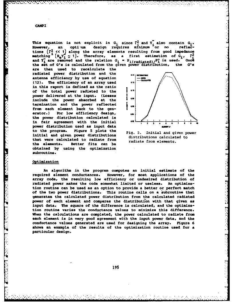
CAMPI
This equation is not explicit in Gi since r2 and Y also contain Gi.
However, an opti lum design requires minimum 'or no reflec-tions (r 2 < i ) along the array elements resulting from good impedancematching (ReYi = I). Therefore, as a first estimation of Gi, r2
and Y- are removed and the relation Gi Pi(radiated)/P is used. Oncethe set of Gts is calculated from the given power distribution, the G'sare then used to recalculate theradiated power distribution and the 6.14 .antenna efficiency by use of equation - ;
*', (12). The efficiency of an array used ,in this report is defined as the ratio * /of the total power radiated to the "power delivered at the input. (Lossesinclude the power absorbed at thetermination and the power reflected jfrom each element back to the gen- •erator.) For low efficiency design, SM
the power distribution calculated isin fair agreement with the initial 3 4 * , I , -power distribution used as input data mF.
- to the program. Figure 5 plots the Fig. 5. Initial and given power* initial and given power distributions distributions calculated to
that were calculated to radiate from radiate from elements.the elements. Better fits can beobtained by using the optimizationsubroutine.
Optimization
An algorithm in the program computes an initial estimate of therequired element conductances. However, for most applications of thearray code, the resulting low efficiency or undesired distribution ofradiated power makes the code somewhat limited or useless. An optimiza-tion routine can be used as an option to provide a better or perfect matchof the two power distributions. This routine calls on a subroutine thatgenerates the calculated power distribution from the calculated radiated
-*.power of each element and compares the distribution with that given asinput data. The square of the difference is calculated, and the optimiza-
* tion routine varies the conductance values to minimize this difference.When the calculations are completed, the power calculated to radiate fromeach element is in very good agreement with the input power data, and the
* conductance values generated are used for designing the array. Figure 6shows an example of the results of the optimization routine used for aparticular design.
i19
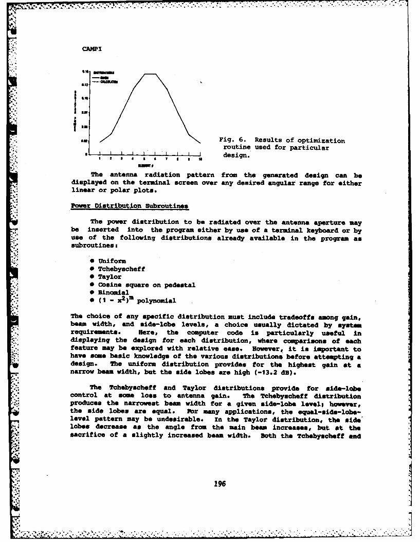
-,, - . . . . . . . . . . . . . . . . . . - -
LICAMPIN
°, 11
LIE
ILI
to m Fig. 6. Results of optimizationroutine used for particular
. I I I I a I design.
The antenna radiation pattern from the generated design can bedisplayed on the terminal screen over any desired angular range for eitherlinear or polar plots.
Power Distribution Subroutines
The power distribution to be radiated over the antenna aperture maybe inserted into the program either by use of a terminal keyboard or byuse of the following distributions already available in the program assubroutines:
- * Uniform0 Tchebyscheff* Taylor
.0 Cosine square on pedestal* Binomial* (1 - X2)m polynomial
The choice of any specific distribution must include tradooffs among gain,beam width, and side-lobe levels, a choice usually dictated by systemrequirements. Here, the computer code is particularly useful indisplaying the design for each distribution, where comparisons of eachfeature may be explored with relative ease. However, it is important tohave some basic knowledge of the various distributions before attempting adesign. The uniform distribution provides for the highest gain at anarrow beam width, but the side lobes are high (-13.2 dB).
The Tchebyscheff and Taylor distributions provide for side-lobecontrol at some loss to antenna gain. The Tchebyscheff distributionproduces the narrowest beam width for a given side-lobe levels however,the side lobes are equal. Pbr many applications, the oqual-side-lobe-level pattern may be undesirable. In the Taylor distribution, the side'lobes decrease as the angle from the main beam increases, but at thesacrifice of a slightly increased beam width. Both the Tchebyscheff and
196
CAMPI
Taylor distributions enable the designer to select a desired side-lobelevel and to compute the element excitation values in terms of a parameterrelated to the side-lobe level.
The distribution of cosine square on a pedestal is a truncateddistribution in which the ratio of the pedestal height to the distributionpeak determines the side-lobe level. The binomial distribution producesno side lobes, but at the expense of low gain and wide beam widths. Thepolynomial distribution provides for a class of distributions in whichfurther tradeoffs among gain, beam widths, and side lobes can be studiedsimply by varying the factor m in the polynomial.
The variety in aperture distributions offered by this program shouldprovide for most systems needs. New or unique distributions can be addedeasily to the existing program as subroutines to expand the scope of thisdesign code.
Antenna Designs
Several linear and planar arrays were designed by using themicrostrip computer model. Figure 7 shows a microstrip S-band array thatwas successfully designed to exhibit the same antenna characteristics(except for polarization) as those derived from the slotted waveguidearray. The microstrip array, however, is N-plane polarized along thearray direction, and the waveguide array is H-plane polarized. & numberof linear arrays were combined by use of a corporate-feed structure toform a planar array as shown in figure 8. Figure 9 shows a polar plot ofthe antenna radiation pattern for both the E-plane (series-feed direction)and the H-plane (corporate-feed direction) polarizations. The success atdesigning microstrip antennas at microwave frequencies prompted an arraydesign for use at around 100 GHz. Figure 10 shows the array mounted in atest fixture, and figure 11 shows the linear plot for both the theory andexperimental results.
Fig. 7. Microstrip antenna designed to have charac-teristics similar to those of waveguide array shownabove.
[ 4
197
L * . °. - . . . ...
cmwi
Pig. S. Microstrip planar array.
u. II) go.0
Fig. 9. Polar plots of antenna radiation patterns:(a) E-plane and (b) H-plane.
198
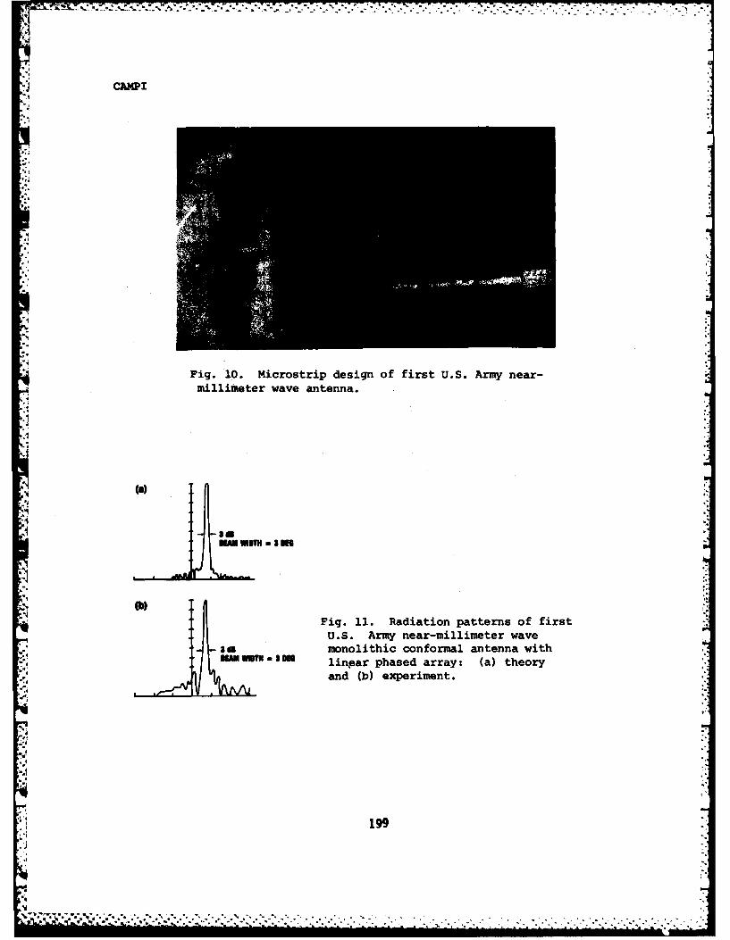
CAMPI
Fig. 10. Microstrip, design of first U.S. Army near-millimeter wave antenna.
"1 IMg3
Fig. 11. Radiation patterns of firstU.S. Army near-millimeter wave
:a3d monolithic conformal
antenna with
umW iuua liripar phased array: (a) theory
and (b) experiment.
Conclusions and Recommendations
By using a simple transmission line model of shunt conductance
elements along with present computer programming techniques, linear array
microstrip antennas can now be simulated, designed, and studied in a shorttime and at a low cost. Measurements of resonant frequency and beam angleof all the antennas fabricated show excellent correlation with the design
data Lubmitted to the computer. Cross polarization of the fields and
mutual coupling of the array elements appear to be minimal. Several
antennas etched by using the same negative have shown identical return-loss measurements and radiation patterns indicating excellentreproducibility.
Additional work is needed in obtaining a better analytical model and
data on the element values of conductance and insertion phase as afunction of patch width, characteristic impedance, and loading. Whenincorporated with an ABCD parameter and transmission matrix calculations,this approach should improve the antenna side-lobe levels and the overallmeasured design performance. Additional information must be gathered tobetter describe the radiation pattern and the directivity of a singlepatch element. Further, it would be desirable to design series arrayshaving elements of equal widths, but with different characteristicimpedance lines interspaced between them. This design would provide for asimpler means of phase shifting the array since the insertion phase ofeach element is the same. Additionally, information about thick and low-lose substrates is needed so that arrays may be better designed to 100GHz, where most of the comonly used dielectrics have thicknessesapproaching the dimensions of one wavelength.
References
(1) A. G. Derneryd I33 Trans. Antennas Propag. AP-24, Nov 1976,846-851o
(2) I. G. Bahl and P. Shartia, Microstip Antennas, Artech House,Inc., 1980.
(3) T. Metzler, Proc. Workshop on Printed Circuit AntennaTechnology, New Mexico State Univ., Las Cruces, Oct 1979, pp 20/1-16.
(4) P. P. Jedlicka and K. R. Carver, Proc. Workshop on PrintedCircuit Antenna Technology, New Mexico State Univ., Las Cruces, Oct 1979,pp 4/1-19.
S4-(5) P. P. Jedlicka and K. R. Carver, Er Trans. Antennas Propag.AP-29, Jan 1981, 147-149o
200
?,; -..-~~~~~~~~~~~~~.. .....--.m.-.--"..,..-.. _,.-...- «.,:.-..., ., .,....-.-.1
CASLAVSKY VIECHNICKI
5'
Resolution of Factors Responsible for Difficulty inGrowing Single Crystals of YAG
*Dr. Jaroslav L. Caslavsky and Dr. Dennis J. ViechnickiArmy Materials and Mechanics Research Center
Watertown, Massachusetts 02172
INTRODUCTION:In a ternary system like Al 0-Y 20 -Nd 0 it is naturally realistic
to expect that numerous factors wY cotri~u ~e each in its own way,to the complexity of growth problems of Nd:YAG single crystals whichis a compound in the ternary system. However, extensive experimentalstudy indicates that not many factors but rather a single factor hascaused a derogative influence on the growth of Nd:YAG single crystals.DEFINITION OF THE PROBLEM:
In 1980, Caslavsky and Viechnicki (1) reported that after meltingof YAG, the structure of the melt undergoes a change, i.e., in spiteof congruent melting of YAG there is no equilibrium between the solidand molten YAG. The non-equilibrium condition occurs on account ofcoordination change of 3/5 of the aluminum ions, which in the solidYAG structure are present in four-fold coordination, while in the meltthey increase their coordination to six. On cooling such a melt, inwhich all YAG nuclei were destroyed, the coordination change is irrevers-ible and the melt of YAG composition begins to solidify at 1855 0 C whereyttrium aluminate (perovskite) commences to solidif as a metastableproeutectic phase. The solidification ends at 170o C as a metastableeutectic mixture of 23.0 mol% Y2 02 and 77.0 mol% Al 0 On the otherhand, if a YAG nucleus, say a seed crystal, is presen in the melt andlatent heat of solidification is slowly withdrawn from the solid-liquidinterface through the seed crystal, the YAG structure will perpetuatefrom the seed crystal on account of the melt converting into a YAG singlecrystal. It also was reported if the rate of solidification increasesover a certain rate; precipitation of metastable proeutectic phase occurs
and the amount formed is directly proportional to the rate of solidifi-cation. Further, it was suggested that presence of neodymia in themelt, as a dopant, somehow de-stabilizes four-fold coordination of thealuminum ions, therefore, the amount of second phase in the presenceof neodymia increases with the rate of crystallization more rapidlythan in the undoped melt.
201
:K.:. ................................. - ...... ..... -..... .s.... .

CASLAYSKY, VIECHNIICKI
To understand this phenomena, futher experimental evidence toexplain the enhanced formation of scattering centers in doped YAG crys-tals was sought and is described in this paper.EXPERIMENTAL METHODS:
a) Growth of the Single Crystals by the Vertical Solidificationof the Melt (VSOM):
In this technique a cylindrical crucible of approximately 75 mmdiameter and 125 mm height is used as a container. The seed crystalis placed in the middle of the bottom of the crucible which then isfilled with the material to be melted. The crucible is positioned withits center on a water cooled heat sink, which in addition to servingas a support for the crucible, prevents the seed crystal from beingmelted and provides the means for controlled latent heat removal ofsolidification during the period of the crystal growth. Since the heatsink is now in the exact center of the cylindrical heating element,the crucible is heated evenly in the circumference, but there is anupward thermal gradient built into the element which is consequentlyreflected in the melt. Unlike most other crystal growth techniques thereare no moving parts .in the VSOM crystal growth technique. The drivingforce for crystallization in this technique is derived from the motionof the thermal field throughout the hot zone of the furnace. Eliminationof moving parts combined with the upward thermal gradient in the meltgives to the VSOM technique a unique stabilization condition, i.e.,
".'- there is practically no thermally induced flow inside the melt, andmechanically produced vibrations are absent.
"- b) The Optical Differential Thermal Analyses (ODTA):This technique was well described in (1) and since during the
course of this investigation it was used only as a supporting methodthe reader is referred to the pertinent publication.
c) Experimental technique to reveal the influence of NdAlO3 onthe Solidification of Nd:YAG Melt:
From the figure la and lb it is apparent that when the growth para-meters are well controlled, the difference in the amount of scatteringcenters in single crystals of YAG and Nd:YAG grown by VSOM method arein both cases minimized or absent. Therefore, to study the factorsresponsible for the formation of second phase particles from singlecrystals is difficult. Owing to this fact it was decided to study thedifferences of solidification of unseeded doped and undoped melts ofYAG composition.
Except for the absence of the seed crystal, the solidificationprocess was exactly the same like it is used by growing single crystalsby VSOM technique. The 75 x 125 mm molybdenium crucible was filledwith material prepared by a process developed for the preparation ofcharges for growing YAG crystals as described in (2). The cruciblewas placed in VSOM crystal growth furnace and heated at a rate of 50°C/h
[ 202
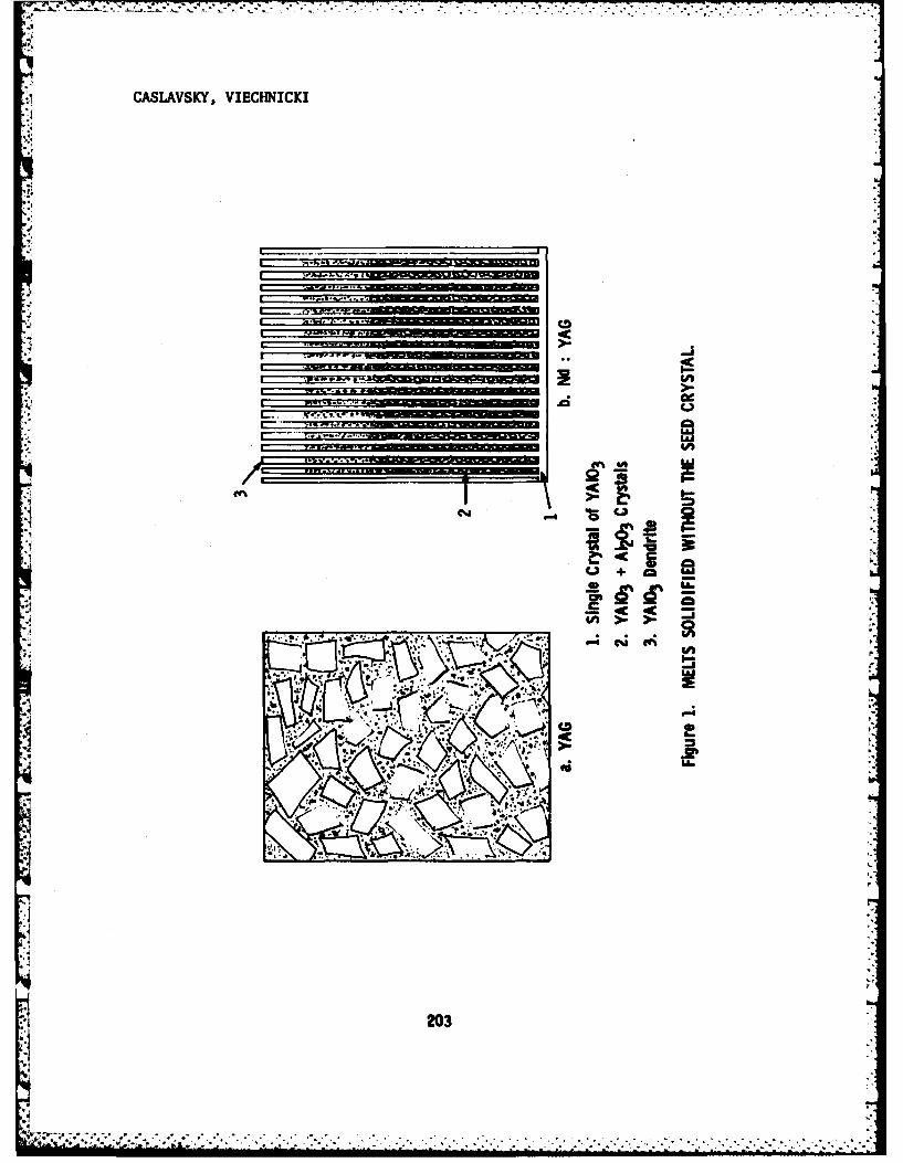
CASLAVSKYJ, VIECHNICKI
41A
~ a IE~Ecc
. -.. I -3_ _ _t t.,
_____________ ini~u~u uI >
0203
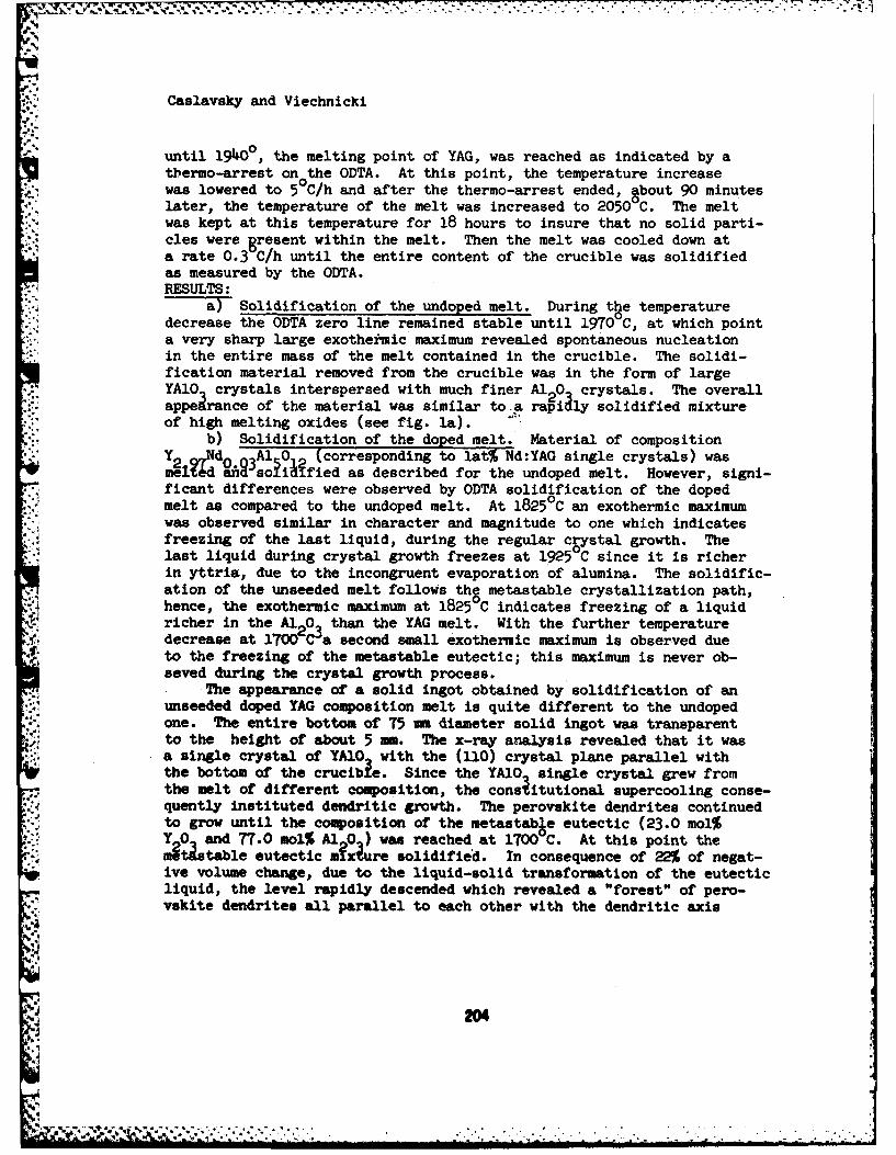
"4
Caslavsky and Viechnicki
until 1940O, the melting point of YAG, was reached as indicated by athermo-arrest on the ODTA. At this point, the temperature increasewas lowered to 5°C/h and after the thermo-arrest ended, about 90 minutes
later, the temperature of the melt was increased to 20500 C. The melt, . was kept at this temperature for 18 hours to insure that no solid parti-
cles were gresent within the melt. Then the melt was cooled down ata rate 0.3 C/h until the entire content of the crucible was solidifiedas measured by the ODTA.RESULTS:
a Solidification of the undoped melt. During the temperaturedecrease the ODTA zero line remained stable until 19700C, at which pointa very sharp large exothermic maximum revealed spontaneous nucleationin the entire mass of the melt contained in the crucible. The solidi-fication material removed from the crucible was in the form of largeYA1O crystals interspersed with much finer Al crystals. The overallapperance of the material was similar toga rapily solidified mixtureof high melting oxides (see fig. la).
V- b) Solidification of the doped melt. Material of compositionY2 Ndo_3Al1 (corresponding to lat% Nd:YAG single crystals) wasmel&d anso ified as described for the undoped melt. However, signi-ficant differences were observed by ODTA solidification of the dopedmelt as compared to the undoped melt. At 1825°C an exothermic maximumwas observed similar in character and magnitude to one which indicatesfreezing of the last liquid, during the regular crystal growth. Thelast liquid during crystal growth freezes at 19250C since it is richerin yttria, due to the incongruent evaporation of alumina. The solidific-ation of the unseeded melt follows the metastable crystallization path,hence, the exothermic maximum at 1825 C indicates freezing of a liquidricher in the AI203 than the YAG melt. With the further temperaturedecrease at 1700 C a second small exothermic maximum is observed dueto the freezing of the metastable eutectic; this maximum is never ob-seved during the crystal growth process.
'The appearance of a solid ingot obtained by solidification of anunseeded doped YAG composition melt is quite different to the undopedone. The entire bottom of 75 mm diameter solid ingot was transparentto the height of about 5 mm. The x-ray analysis revealed that it wasa single crystal of YA1O with the (110) crystal plane parallel withthe bottom of the crucible. Since the YA1O single crystal grew fromthe melt of different composition, the consitutional supercooling conse-quently instituted dendritic growth. The perovskite dendrites continuedto grow until the composition of the metastable eutectic (23.0 mol%Y 0 and 77.0 mol% Al 0 ) was reached at 170O0 C. At this point themetstable eutectic mx ure solidified. In consequence of 22% of negat-ive volume change, due to the liquid-solid transformation of the eutecticliquid, the level rapidly descended which revealed a "forest" of pero-vskite dendrites all parallel to each other with the dendritic axis
204
CASLAVSKY, VIECHNICKI
in the [001] direction. This indicated that all of the densities wereseededby the single crystal found on the bottom of the ingot. The meta-stable eutectic mixture was found in the spaces among the dendrites(see fig. lb).
These experiments were repeated three times with the same results;the reproducibility of the experiments and their interpretation ledto a mechanism of scattering centers formation in Nd:YAG single crystals.EXPLANATION OF FORMATION OF SCATTERING CENTERS:
In the solid state the YAG structure, from the oxides componentsAl 0 and Y20 , forms quite easily at temperatures as low as 7000 C.Tlje kinetis~of formation of the YAG structure is directly proportionalto the temperature, and at the temperatures between 1700 C and 18000Cthe stoichiometric mixture of the oxides reacts completely in two hoursto the YAG structure. By contrast, when the oxide mixture is meltedand then solidified no YAG is formed. This phenomenon is seen whetheror not Nd2 0 is present. Nevertheless, if the melt is seeded and solidi-fication performed under the controlled conditions, a single crystalof YAG is obtained. However, the experimentally determined growth ratesneeded to obtain scattering center free doped crystals, are at leastthree times lower than the growth rates for undoped crystals.
In reference (1) it was established that it was impossible to formYAG from an unseeded melt due to the fact that the aluminium ions arenot willing to lower their coordination without external influence andwill much rather form incongruently melting perovskite even from non--stoichiometric melt. The only mechanism which forces aluminum ionsto the four-fold coordination is the dangling bonds protruding fromthe free surface of the seed crystal. Such dangling bonds in the mostfavored case can extend from the solid structure of the YAG only 12A.Therefore, the coordination change can take place only in close prox-imity to the free surface of the seed crystal. If the solidificationrate exceeds the rate with which the coordination change can take place,the perovskite phase will crystallize simultaneouslywith the YAG. Fromall experimental work it is evident that the rate of change of the alumi-num ions is the factor controlling the rate of the YAG structure forma-tion. If this would be the only factor responsible for formation ofthe scattering centers in YAG, there should be no reason for Nd:YAGto grow scattering center free only at much lower rates than undopedYAG. From the experiments described in the previous paragraph, thefollowing conclusion for enhanced formation of scattering centers inNd:YAG is interpreted as follows:
YAlO-perovskite is the highest melting compound in the ternarysystem melting congruently without decomposition at 2110°C. It is high-ly probable in this ternary system that under sufficient supercoolingNdAlO will first form stable or supercritical nuclei, and this factaccouQts for the difference in the crystallization behavior of unseeded
A.°
] "205
'
-, V ~ . . *.. . .. . . . . .
Caslavsky and Viechnicki
doped and undoped melts of YAG composition.In the VSOM crystal growth arrangement the melt around the bottom
part of the crucible nearest the heat sink is estimated to be coolerby 1000 to 150°C than the melt farther away from the heat sink. Duringslow cooling of a melt of Nd:YAG composition there is enough time, inthe locally supercooled area, for NdAlO to nucleate and eventuallyform supercritical nuclei. With progreising cooling such nuclei willgrow. However, in this melt there is not enough neodymium ions to sus-tain the growth of NdAlO but since NdAlO is istostructural with YalO3a heteroepitaxial boundary will be formed and YA1O will continue togrow off as a single crystal until the constitutioAal supercooling willforce dendritic growth.
In the VSOM technique it is impossible experimentally to measurethe thermal Kradient near the solid-liquid interface, but from experi-ence gained working with this technique, it has been found that to con-trol growth, the thermal gradient near the interface has to be verysteep. In such steep gradient, however, nucleation of the NdAlO stillcan occur according to a reaction
L . .L .+ S ....... ....................... (1)where L is a liquid free of any solid particles while L is liquid1 2whose composition has changed due to the nucleation of S = NdAl..Therefore, if the rate of the growth of Nd:YAG exceeds the trans~ortrateof solid particles so that they cannot be carried away from the solid-liquid interface into the melt region where temperature is high enoughto reverse reaction (1) to:
L2 + S = L1 . . ........... (2)
then the NdAlO particles will deposit by gravity on the solid partof the solid-liquid interface and will be embedded in it and will formscattering centers in the resulting single crystal.CONCLUSIONS:
The enhanced formation of the scattering centers in Nd:YAG is attri-buted to the fact that the melting point of YAG is 170 C lower thanthe melting point of NdAlO . Further, since aluminium ions in theneodyium aluminate are preaent in six-fold coordination NdAlO can easilynucleate near the solid-liquide interface where lower tempera ure favors
reaction (1). Provided that the growth rate of Nd:YAG exceeds the kin-etics of reaction (2), the second phase particles will precipitate inthe growing Nd:YAG crystal and appear as scattering centers.
From the experimental evidence it can be concluded that in thecomposition section on and near the tie line connecting NdAlO and Y Al
in the Nd 0 -Y20 -Al O ternary system, NdAlO shows an inAerentproperty to nuleat firs . To eliminate the nugleation of NdAlO duringthe crystal growth of Nd:YAG the thermal gradient near the solid-liquidinterface has to be very steep while the melt temperature has to bekept above the temperature which prevents reaction (1). Simultaneously
2 206
1:2 . . .. . . . . . . . . . . . . . . . . . . . ... ..
- .!
Caslavsky and Viechnicki
the speed of the interface advancement has to be set below the thermally
induced flow of the melt from the solid-liquid interface. Therefore,
it is apparent that with the correct growth conditions scattering center
free Nd:YAG single crystals can be grown by VSOM.
REFERENCES:1. Caslavsky, J.L., Viechnicki, D.J., Journal of Material Science 15(1980) 1709.2. Viechnicki, D.J., Caslavsky, J.L., American Ceramic Society Bulletin58 (1979) 700.
7.2
207
Ul
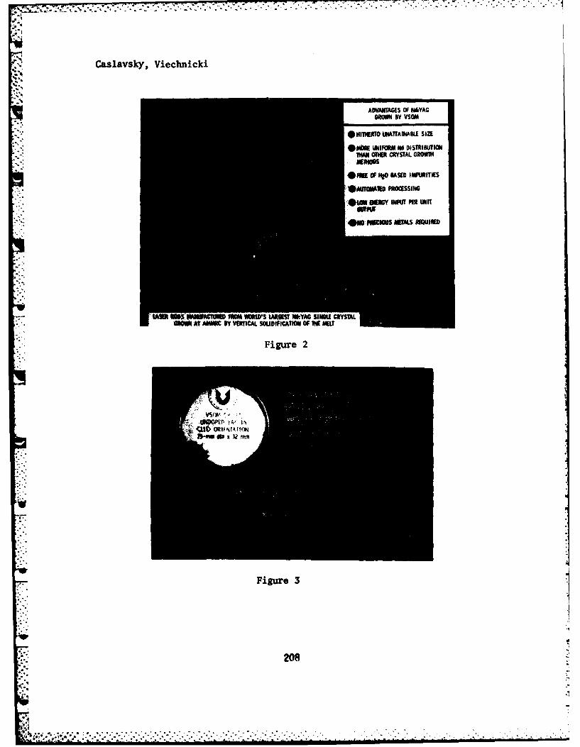
Caslavsky, Viecimicki
hO~~~~~~~~~~lGO AT *11 V ETCL OSFCAINO TEI
FigureNAtANAL 2IZ
OW NFR dDSRBTOrAANOM CYSTA GRO
208 FM2 AE IPRTE
..................... IE P.. .. ... .. .. ... .NG
4a OEM ow Put UNI
CHAPIN, CONLEY & JAMISON
GENERATION OF A SYSTEM WHICH EXIBITS ANISOPYCNIC IN THE CONVERSION OF ARMYVEHICLES TO SILICONE BRAKE FLUID (1)
*MR. CHARLES C. CHAPINMR. JAMES H. CONLEY
MR. ROBERT G. JAMISONUS ARMY MOBILITY EQUIPMENT RESEARCH AND DEVELOPMENT COMMAND
FORT BELVOIR, VA 22060
The US Army has been using three different automotive hydraulic brakefluids covered by Federal Specification VV-B-680, for use in all Tank-Auto-motive equipment (temperate -tropical areas), Military Specification MIL-H13910 for arctic use, and Military Specification MIL-P-46046 for preser-vative use (2). These polyglycol and castor oil type fluids are hygroscopicand absorb water while in use which adversely affects their performance by
* lowering the vapor lock temperature, increasing the low temperature vis-cosity, and by contributing to component corrosion which can lead to cupscoring, as well as system failure.
In 1967 the US Army began developing a single multipurpose siliconebased brake fluid which would overcome the absorption of water exibited bythe conventional fluids as well as provide all weather and preservativeproperties. This one fluids, which replaces the three existing fluids, can-reduce logistics and maintanence costs. Any vehicle (quipped with thisfluid will be ready for use itA any geographical area at a moments notice.Therefore, vehicles could be moved from the tropics to the arctic or couldbe put into storage without requiring any other current brake systemmaintanence procedures (3).
Brake Fluid, Silicone (BFS), Military Specification MIL-B-46176, whichwas developed by MERADCOM (4) in conjunction with industry was approved forArmy use in 1980. All tactical vehicles, administrative use vehicles, com-mercially procured vehicles, construction equipment and material handlingequipment which currently use polyglycol type fluids will be converted tosilicone brake fluid by July 1982.
The wipe and clean procedure for conversion, which was successfullytested at Yuma Proving Grounds, Arctic Field Test Center, Panama TropicTest Center (5) and was the recommended conversion method, was found to beunacceptable due to the labor intensiveness of the procedure, its impli-cations to manpower requirements and cost. An alternate method (6) forbrake fluid replacement, the flush and fill procedure (adapted for TB43-
209
CHAPIN, CONLEY, & JAMISON
0002-87) was approved for use based on these same considerations. Astraight flush and fill procedure was tested by MERADCOM (7) and found tobe inefficient for the following interdependent reasons:
a. The geometry of the wheel cylinders (bleeder valves at the top).b. The immiscibility of the two types of fluid.c. The lower density of the silicone relative to the polyglycol.
Figure I shows a cross-section of each of the wheel cylinder types anda caliper. The inlet lines and bleeder valves are indicated. The bleedervalves are always positioned at the uppermost point of the wheel cylinderto allow the lower density air to be bled from the system.
The results of testing of straight flush/fill procedure indicated thatfor the M-151 (jeep) vehicles, the procedure removed essentially all ofthe polyglycol. However, the other wheel cylinders (and calipers) do nothave inlet lines located at the bottom of the cylinder and the methodleaves residual polyglycol trapped in the system. Since inlet lines arein the middle of the cylinder, the fluid simply overlayers the polyglycolafter removing the accessible polyglycol by displacement.
An ILIR project was initiated at MERADCOM to address this problem ex-perimentally and to subsequently develop a cost-effective method whichwould achieve complete polyglycol removal.
Approach
Since the straight flush/fill method gave a liquid binary phase system(silicone polyglycol) a solution approach was used to reverse the phasestructure by the inclusion of an intermediate fluid of sufficiently lowdensity. To achieve a reversal of the phases, a fluid must be selectedfor which the ternary system will exibit an isopycnic tie line (8). Theisopycnic tie line (or twin density tie line as it is called in multi-component systems) is that tie line at which the densities of the twophases are equal (a zero density difference). Upon passing the isopycnicline the density difference for the two phase undergoes a sign change(plus to minus or visa versa) and the phases are reversed, the upper be-coming the lower and the lower becoming the upper.
The approach was, then to select a fluid which would generate an iso-pycnic in the silicone-polyglycol system with as high a phase boundaryas possible (so that two phases will form under the various conditionsfound in the different wheel cylinders and calipers). This intermediatefluid must also be a cosolvent for the silicones and the polyglycols,have a high boiling point, be non-corrosive, non-hygroscopic, non-toxic,non-flammable, be inexpensive, and must be compatible with the elastomersin brake systems.
210
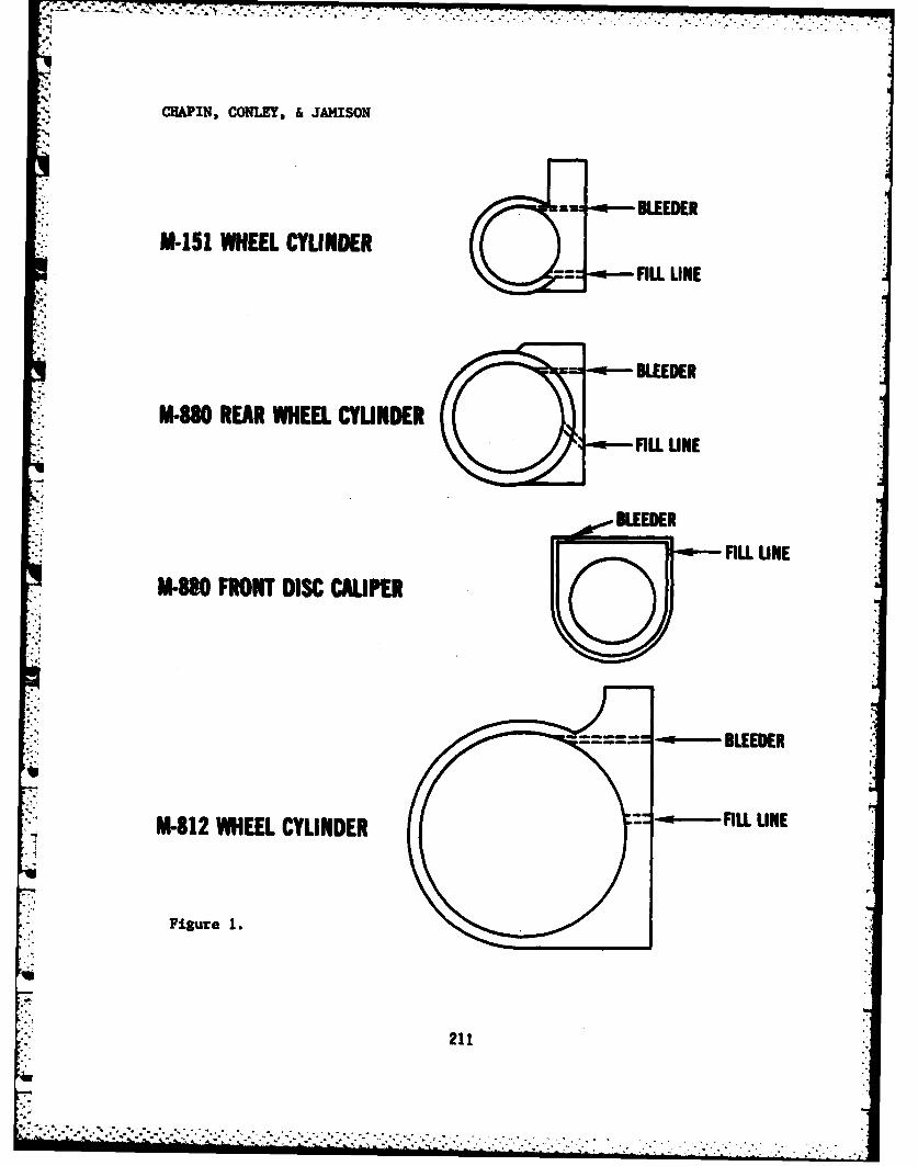
CHAPIN, CONLEY, & JAMISON
BLEEDER
AM-151 WHEEL CYLINDERd:: FLLULNE
M-880 REAR WHEEL CYUINDER
5EDER FIL LINE
M-88 FRONT DISC CALIPER
- ---- -- BLEEDER
M-812 WHEEL CYLINDER -w RLIN
Figure 1.
211
...............
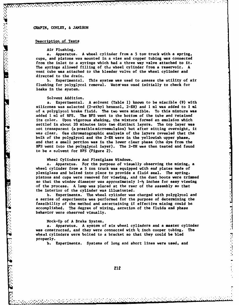
. 7 7 . .7 . -. * . .
HAPOIN, CONLEY, & JAMISON
Description of Tests
Air Flushing.a. Apparatus. A wheel cylinder from a 5 ton truck with a spring,
cups, and pistons was mounted in a vise and copper tubing was connectedfrom the inlet to a syringe which had a three way valve attached to it.The syringe allowed filling of tha wheel cylinder from a reservoir. Avent tube was attached to the bleeder valve of the wheel cylinder anddirected to the drain.
b. Experimental. This system was used to assess the utility of airflushing for polyglycol removal. Waterwas used initially to check forleaks in the system.
Solvent Addition.a. Experimental. A solvent (Table 1) known to be miscible (9) with
silicones was selected (2-ethyl hexanol, 2-EH) and 1 ml was added to 1 mlof a polyglycol brake fluid. The two were miscible. To this mixture wasadded I ml of BFS. The BFS went to the bottom of the tube and retainedits color. Upon vigorous shaking, the mixture formed an emulsion whichsettled in about 20 minutes into two distinct layers. The top layer wasnot transparent (a possiblemicroemulsion) but after sitting overnight, itwas clear. Gas chromatographic analysis of the layers revealed that thebulk of the polyglycol and the 2-ER were in the yellowish upper phase,and that a small portion was in the lower clear phase (the dye from theBFS went into the polyglycol layer). The 2-EH was then tested and foundto be a solvent for BFS (Figure 2).
Wheel Cylinders And Plexiglass Windows.a. Apparatus. For the purpose of visually observing the mixing, a
wheel cylinder from a 5 ton truck was equipped with end plates made ofplexiglass and bolted into place to provide a fluid seal. The spring,pistons and cups were removed for viewing, and the dust boots were trimmedso that the window diameter was approximately 1-h inches for easy viewingof the process. A lamp was placed at the rear of the assembly so thatthe interior of the cylinder was illuminated.
b. Experiments. The wheel cylinder was charged with polyglycol anda series of experiments was performed for the purpose of determining thefeasibility of the method and ascertaining if effective mixing could beaccomplished. The degree of mixing, aeration of the fluids and phasebehavior were observed visually.
Mock-Up of A Brake System.a. Apparatus. A system of six wheel cylinders and a master cylinder
was constructed, and they were connected with inch cooper tubing. Thewheel cylinders were bolted to a bracket so that they could be bledproperly.
b. Experiments. Systems of long and short lines were used, and
212
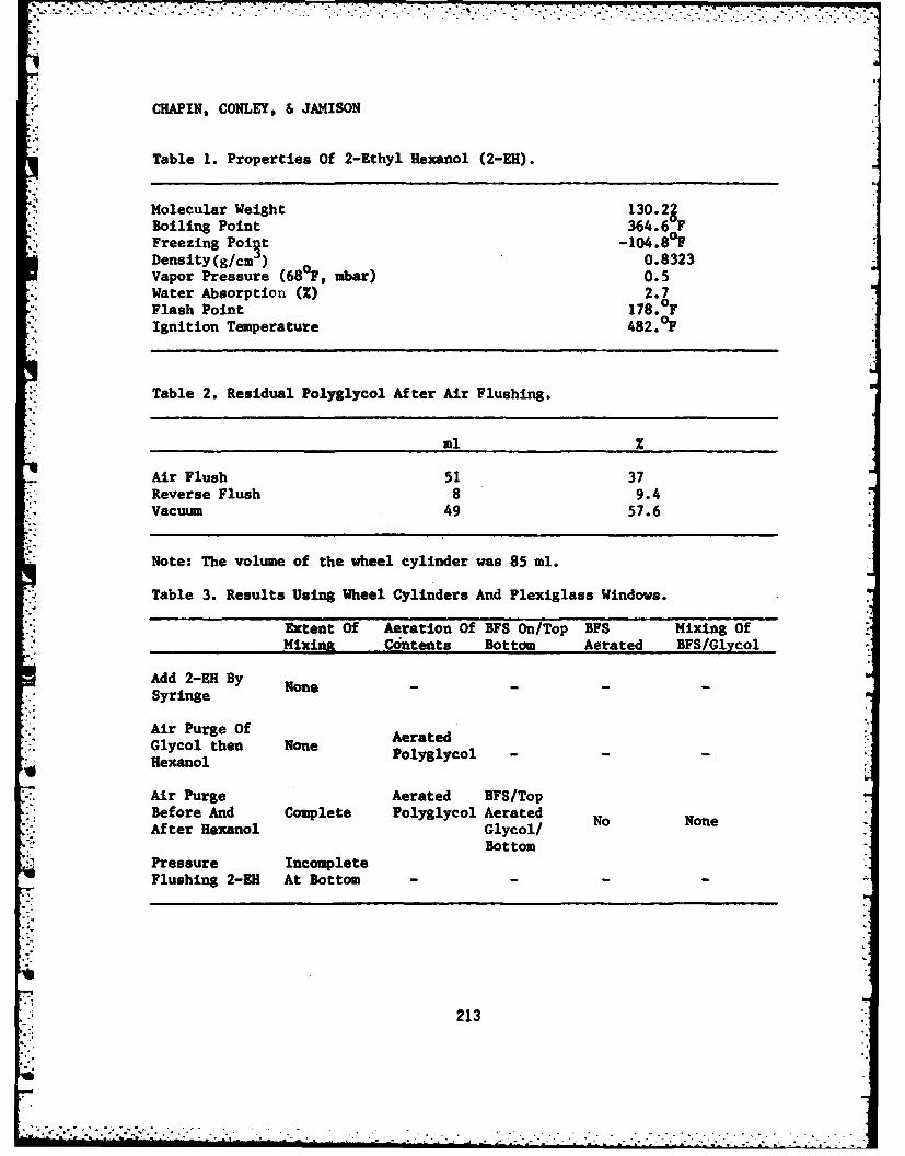
*. .
CHAPIN, CONLEY, & JAMISON
Table 1. Properties Of 2-Ethyl Hexanol (2-EH).
Molecular Weight 130.2, Boiling Point 364.6F
Freezing Poit -104.8 0 FDensity(g/cm) 0.8323Vapor Pressure (680F, mbar) 0.5Water Absorption (1) 2.7Flash Point 178.FIgnition Temperature 482. °1
*. Table 2. Residual Polyglycol After Air Flushing.
ml Z
Air Flush 51 37Reverse Flush 8 9.4Vacuum 49 57.6
Note: The volume of the wheel cylinder was 85 ml.
Table 3. Results Using Wheel Cylinders And Plexiglass Windows.
* Extent Of Aeration Of BFS On/Top BFS Mixing Of' Mixing Cntents Bottom Aerated BFS/Glycol
Add 2-EH By NoneSyringe
Air Purge OfGlycol then None Aerated
Hexanol Polyglycol --Hexanol
Air Purge Aerated BFS/TopBefore And Complete Polyglycol AeratedAfter Hexanol Glycol/
BottomPressure IncompleteFlushing 2-EH At Bottom
213
CHAPIN, CONLEY, & JAMISON
IC
1-4 ac-
P. 0 j
, 0
'., 2 1 4
", -y.

CHAPIN, CONLEY, & JAMISON
different flushing volumes of the density modifier were used to developa method for eventual use in the conversion of vehicles.
Caliper Experiments.a. Apparatus. A caliper from a commercial vehicle was attached to
the master cylinder with a three foot line, and spacers were clamped intothe caliper to fix the internal volume at 90 ml.
Used Wheel Cylinder.a. Apparatus. A used wheel cylinder from a 5 ton truck was con-
* nected to the master cylinder, and flushing experiments were conductedto determine the effect of the sludkeand the extent of sludge removal forthis process.
Administrative Vehicle Test.a. Apparatus. This vehicle was selected because it had wheel
cylinders and calipers, and because it had over 100,000 miles on it so itcould be expected to be a worst case test.
b. Test. A proposed procedure based on previous experiments wasused and the vehicle converted. This procedure involved purging thesystem with air, flushing the two rear wheel cylinders simultaneously andthen flushing with the 2-EH. The wheel cylinders were flushed with onevolume of the master cylinder (200 ml) and the calipers were flushedindividually with twice this amount of fluid. After the fluid flushes, theair (used for flushing) was allowed to purge the system for one minuteafter the fluid was purged. The vehicle was then pressure bled with BFSwhile allowing a specific volume of the BFS to pass through the system toinsure complete removal of the 2-EH. The wheel cylinders and caliperswere removed for analysis and subsequently replaced.
Demonstration Of The Method.a. Apparatus. This demonstration of the method for TACO involved
the conversion of a 2- ton vehicle and a jeep. A second 2- ton vehiclewas converted on a trial run basis prior to the demonstration. An M-880and a 5 ton truck were available for this demonstration but were not con-verted.
Phase Diagram For The BFS/Polyglycol/2-EH.a. Apparatus. This diagram was prepared by the titration method,
using the fully formulated brake fluids (10).
Infrared Examination Of Hydrogen Bonding Effects.a. The instrument used for the infrared examination of hydrogen
bonding effects in these fluids was a Perkin Elmer 580 using various cella
Results Of Tests
j 215
.11 - * ."*I.. ... o -, .,
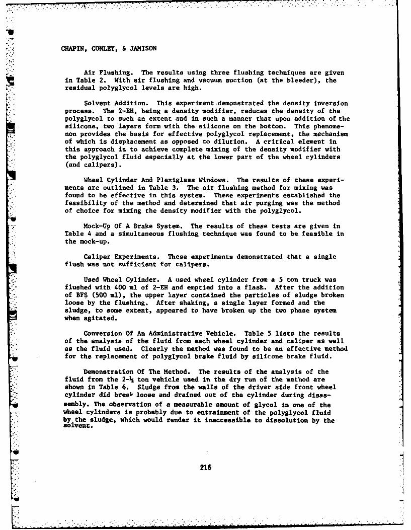
CHAPIN, CONLEY, & JAMISON
Air Flushing. The results using three flushing techniques are givenin Table 2. With air flushing and vacuum suction (at the bleeder), theresidual polyglycol levels are high.
Solvent Addition. This experiment.demonstrated the density inversionprocess. The 2-EH, being a density modifier, reduces the density of thepolyglycol to such an extent and in such a manner that upon addition of thesilicone, two layers form with the silicone on the bottom. This phenome-non provides the basis for effective polyglycol replacement, the mechanismof which is displacement as opposed to dilution. A critical element inthis approach is to achieve complete mixing of the density modifier withthe polyglycol fluid especially at the lower part of the wheel cylinders(and calipers).
Wheel Cylinder And Plexiglass Windows. The results of these experi-ments are outlined in Table 3. The air flushing method for mixing wasfound to be effective in this system. TheRe experiments established thefeasibility of the method and determined that air purging was the methodof choice for mixing the density modifier with the polyglycol.
Mock-Up Of A Brake System. The results of these tests are given inTable 4 and a simultaneous flushing technique was found to be feasible inthe mock-up.
Caliper Experiments. These experiments demonstrated that a singleflush was not sufficient for calipers.
Used Wheel Cylinder. A used wheel cylinder from a 5 ton truck was
flushed with 400 ml of 2-EH and emptied into a flask. After the addition
of BPS (500 ml), the upper layer contained the particles of sludge brokenloose by the flushing. After shaking, a single layer formed and thesludge, to some extent, appeared to have broken up the two phase systemwhen agitated.
Conversion Of An Administrative Vehicle. Table 5 lists the resultsof the analysis of the fluid from each wheel cylinder and caliper as wellas the fluid used. Clearly the method was found to be an effective methodfor the replacement of polyglycol brake fluid by silicone brake fluid.
Demonstration Of The Method. The results of the analysis of thefluid from the 2- ton vehicle used in the dry run of the method areshown in Table 6. Sludge from the walls of the driver side front wheelcylinder did break loose and drained out of the cylinder during disas-sembly. The observation of a measurable amount of glycol in one of thewheel cylinders is probably due to entrainment of the polyglycol fluidby the sludge, which would render it inaccessible to dissolution by thesolvent.
:.'. 216 "
............... .
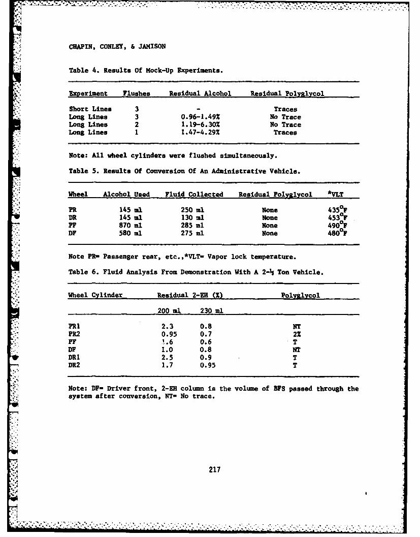
10
CHAPIN, CONLEY, & JAMISON
Table 4. Results Of Hock-Up Experiments...
Experiment Flushes Residual Alcohol Residual PolyglycolShort Lines 3 TracesLong Lines 3 0.96-1.49% No Trace
Long Lines 2 1.19-6.30% No TraceLong Lines I 1.47-4.29% Traces
Note: All wheel cylinders were flushed simultaneously.
Table 5. Results Of Conversion Of An Administrative Vehicle.
Wheel Alcohol Used Fluid Collected Residual Polyglycol *VLT
PR 145 ml 250 ml None 435OFDR 145 ml 130 ml None 4530FPF 870 ml 285 ml None 4900FDF 580 ml 275 ml None 480°F
Note PR- Passenger rear, etc. ,*VLT= Vapor lock temperature.
*1 Table 6. Fluid Analysis From Demonstration With A 2- Ton Vehicle.
Wheel Cylinder Residual 2-EH MZ) Polyglycol
200 ml 230 ml
PRI 2.3 0.8 NTPR2 0.95 0.7 2%PF 1.6 0.6 TDF 1.0 0.8 NTDRI 2.5 0.9 TDR2 1.7 0.95 T
Note: DF= Driver front, 2-EH column is the volume of BFS passed through thesystem after conversion, NT- No trace.
217
q .:: . ' ,."# ,? -s4 , - .. , . ": " .. " '-" ' .' ... ., -. -. " . ..-. .... ". .." -' -'.. . 4.. . -. - - - . - . . . ... .. . . . .
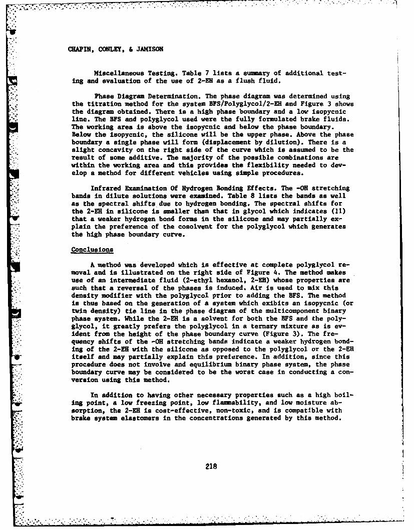
CHAPIN, CONLEY, & JAMISON
Miscellaneous Testing. Table 7 lists a sumuary of additional test-ing and evaluation of the use of 2-EH as a flush fluid.
Phase Diagram Determination. The phase diagram was determined usingthe titration method for the system BFS/Polyglycol/2-EH and Figure 3 showsthe diagram obtained. There is a high phase boundary and a low isopycnicline. The BFS and polyglycol used were the fully formulated brake fluids.The working area is above the isopycnic and below the phase boundary.Below the isopycnic, the silicone will be the upper phase. Above the phaseboundary a single phase will form (displacement by dilution). There is aslight concavity on the right side of the curve which is assumed to be theresult of some additive. The majority of the possible combinations arewithin the working area and this provides the flexibility needed to dev-elop a method for different vehicles using simple procedures.
Infrared Examination Of Hydrogen Bonding Effects. The -OH stretchingbands in dilute solutions were examined. Table 8 lists the bands as well
as the spectral shifts due to hydrogen bonding. The spectral shifts forthe 2-EH in silicone is smaller than that in glycol which indicates (11)that a weaker hydrogen bond forms in the silicone and may partially ex-plain the preference of the cosolvent for the polyglycol which generatesthe high phase boundary curve.
Conclusions
A method was developed which is effective at complete polyglycol re-moval and is illustrated on the right side of Figure 4. The method makesuse of an intermediate fluid (2-ethyl hexanol, 2-EH) whose properties aresuch that a reversal of the phases is induced. Air is used to mix thisdensity modifier with the polyglycol prior to adding the BFS. The methodis thus based on the generation of a system which exibits an isopycnic (ortwin density) tie line in the phase diagram of the multicomponent binaryphase system. While the 2-ER is a solvent for both the BFS and the poly-
*glycol, it greatly prefers the polyglycol in a ternary mixture as is ev-ident from the height of the phase boundary curve (Figure 3). The fre-quency shifts of the -OH stretching bands indicate a weaker hydrogen bond-ing of the 2-EH with the silicone as opposed to the polyglycol or the 2-EHitself and may partially explain this preference. In addition, since thisprocedure does not involve and equilibrium binary phase system, the phaseboundary curve may be considered to be the worst case in conducting a con-version using this method.
In addition to having other necessary properties such as a high boil-ing point, a low freezing point, low flammability, and low moisture ab-sorption, the 2-EH is cost-effective, non-toxic, and is compatible withbrake system elastomers in the concentrations generated by this method.
218
. * . * .
.. . . . .. . . . . . . . . .
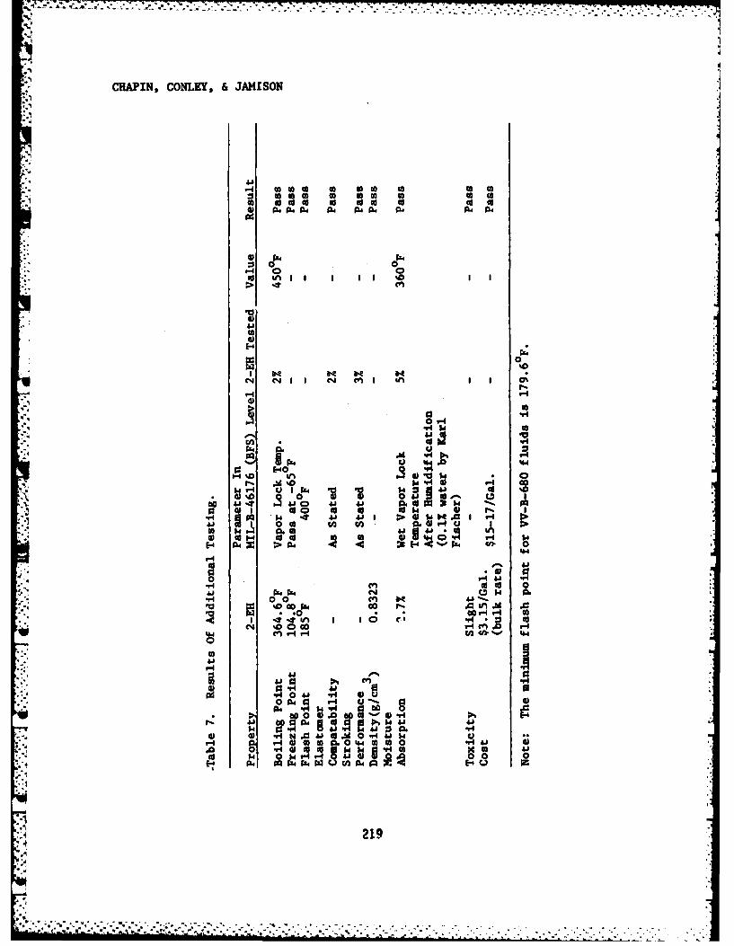
* CHAPIN, CONLEY, & JAMISON
a- Cle 0 41 0 ani 0 cc a01 ;wo 000 02. It 4.
*c Lm I m l I I I OI I
4.1
E-4
0 9-0
N- NI I N 9l I I I 0
. 1 4L 00v t
<.5 4j 1
* '4
41 J44~ C4 0
10 mI-4"4 7-4 (Ak*
4*09- r4 4*4
41.
'-41
0 Q O
0 ,14
.14 0 c000 0100 4 V.4 No0
N " AO0 E-4(I. u -I
4219
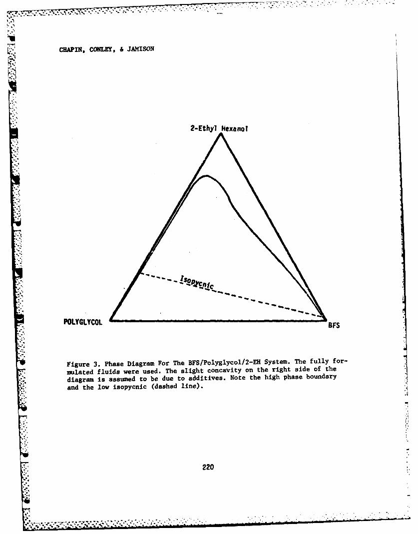
cHApIN, CONLEY, & JAMISON
.J-
2-Ethyl Nexanol
-4.lv-1
POLYGLYCOLBF
Figure 3. Phase Diagram For The BPS/Polyglycol/2-EH System. The fully f or-
mulated fluids were used. The slight concavity on the right side of the
diagram is assumed to be due to additives. Note the high phase boundary
and the low isopycnic (dashed line). -
220
42$
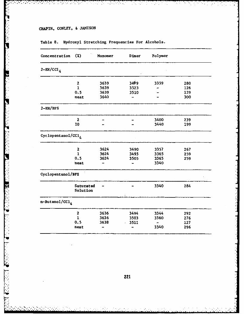
CHAPIN, CONLEY, & JAMISON
Table 8. Hydroxyl Stretching Frequencies For Alcohols.
Concentration ()Monomer Dimer Polymer
2-EH/Cd14
2 3639 3499 3359 2801 3639 3523 - 126
0.5 3639 3510 -129
neat 3640 - -300
2-EH/BFS
2 -- 3400 23910 -- 3440 199
Cyclopentanol/CC14
2 3624 3490 3357 2671 3624 3495 3365 259
0.5 3624 3505 3365 259neat - - 3340
Cyclopentanol/BFS
Saturated -- 3340 284
Solution
n-Butanol/CC1 4
U2 3636 3494 3344 292
1 3636 3503 3360 2760.5 3638 3511 - 127neat - - 3340 296
1w
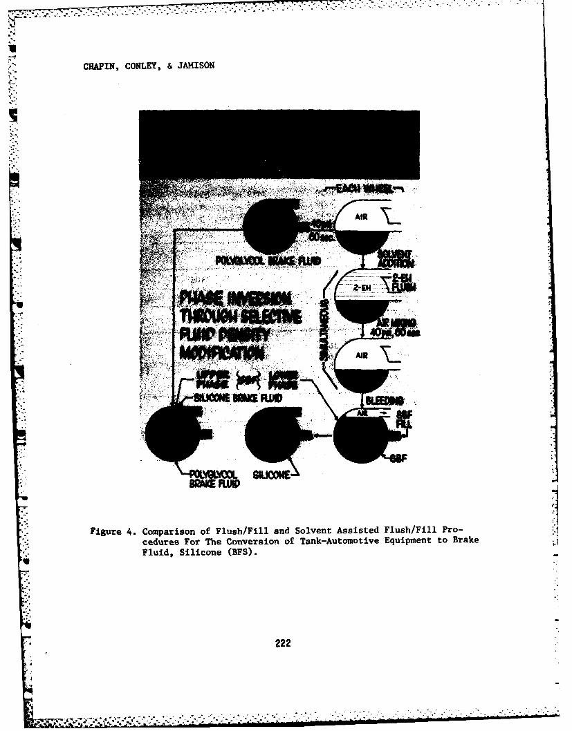
CHAPIN, CONLEY, & JAMISON
AI
AI
Figure 4. Comparison of Flush/Fill and Solvent Assisted Flush/Fill Pro-cedures For The Conversion of Tank-Automotive Equipment to Brake
Fluid, Silicone (BFS).
222
CHAPIN, CONLEY, & JAMISON
The US IC will be using the method (which is being patented) to converttheir shipboard vehicles on board the Near Term Prepositioned Fleet atDiego Garcia to BFS. An extension of the method covering mineral fluidbased systems is being considered by industry. The conversion to BFS is ex-pected to save the US Army $21M over the next 10 years. This method couldnot only recapture the all climate utility and high vapor lock temperatureof BFS but could substantially increase the cost-effectiveness of the con-version.
References
1. Taken in part from the Ph.D. thesis of C.C.C., The American University,Washington, D.C., May, 1982.
2. Federal Specification VV-B-680, Brake Fluid, Automotive, July 20, 1972;Military Specification MIL-H-13910, Hydraulic Fluid, Polar Type, Auto-motive, All Weather, February 3, 1967; Military Specification MIL-P-
* - 46046, Preservative Fluid, Automotive Brake System and Components,August 26, 1964.
3. Conley, J.H., and Jamison, R.G., Army Experience With Silicone BrakeFluid, S.A.E. Technical Paper Series #780660, 1978.
4. Military Specification MIL-B-46176, Brake Fluid, Silicone, Automotive,All Weather, Operational and Preservative, March 27, 1978.
5. Conley, J.H., and Jamison, R.G., Silicone Brake Fluid: One Year FieldTest, MERADCOM Report No. 2132, February 1975.
6. TB43-0002-87, DA Technical Bulletin, Brake Fluid, Silicone (BFS) Con-version Procedures for Tank-Automotive Equipment, May 1981.
7. MERADCOM Letter Report, Evaluation of Flush/Fill Procedures for Sil-
icone Brake Fluid Retrofit, DRDME-GL, October 6, 1980.
8. Francis, A.W., Ind. Eng. Chem., 45, 2789, 1953.
9. Smith, A.L., ed., Analysis of Silicones, Vol. 41, Cemical Analysis Ser-ies of Monographs, Wiley, New York, 1974.
-*' 10.. Francis, A.W., Liquid-Liquid Equilibrtiums, Vol 3, Interscience Lib-.' * rary of Chemical Engineering and Processing, Interscience Publishers,
New York, 1963.
11. Pimentel, G.C., and McClellan, A.L., The Hydrogen Bond, Freeman, SanK Francisco, 1960.
[ 223
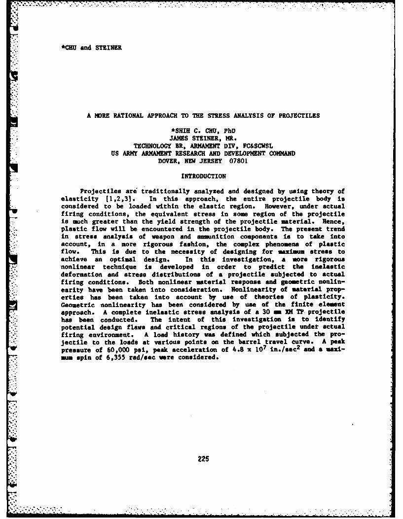
*CHU and STEINER
A MORE RATIONAL APPROACH TO THE STRESS ANALYSIS OF PROJECTILES
*SHIH C. CHU, PhDJAMES STEINER, MR.
TECHNOLOGY BR, ARMAMENT DIV, FC&SCWSLUS ARMY ARMAMENT RESEARCH AND DEVELOPMENT COMMAND
DOVER, NEW JERSEY 07801
INTRODUCTION
Projectiles are traditionally analyzed and designed by using theory ofelasticity [1,2,31. In this approach, the entire projectile body isconsidered to be loaded within the elastic region. However, under actualfiring conditions, the equivalent stress in some region of the projectileis much greater than the yield strength of the projectile material. Hence,plastic flow will be encountered in the projectile body. The present trendin stress analysis of weapon and ammunition components is to take intoaccount, in a more rigorous fashion, the complex phenomena of plasticflow. This is due to the necessity of designing for maximum stress toachieve an optimal design. In this investigation, a more rigorousnonlinear technique to developed in order to predict the inelasticdeformation and stress distributions of a projectile subjected to actualfiring conditions. Both nonlinear material response and geometric nonlin-earity have been taken into consideration. Nonlinearity of material prop-erties has been taken into account by use of theories of plasticity.Geometric nonlinearity has been considered by use of the finite elementapproach. A complete inelastic stress analysis of a 30 sm DI TP projectilehas been conducted. The intent of this investigation is to identifypotential design flaws and critical regions of the projectile under actualfiring environment. A load history was defined which subjected the pro-jectile to the loads at various points on the barrel travel curve. A peakpressure of 60,000 psi, peak acceleration of 4.8 x 107 in./sec2 and a maxi-mum spin of 6,355 rad/sec were considered.
225
,
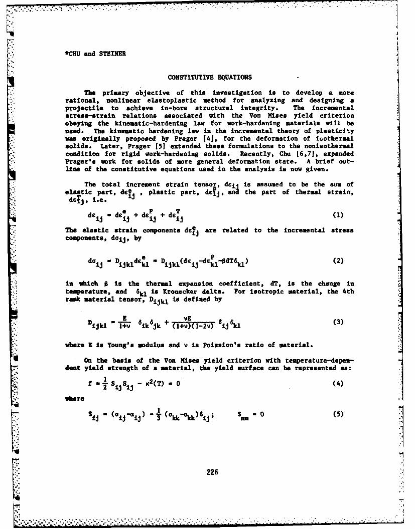
p ., , . -- ! _ -| ! g ] i - -1 ' -
*CHU and STEINER
CONSTITUTIVE EQUATIONS
The primary objective of this investigation is to develop a morerational, nonlinear elastoplastic method for analyzing and designing aprojectile to achieve in-bore structural integrity. The incrementalstress-strain relations associated with the Von mases yield criterionobeying the kinematic-hardening law for work-hardening materials will beused. The kinematic hardening law in the incremental theory of plasticitywas originally proposed by Prager [4], for the deformation of isothermalsolids. Later, Prager [5] extended these formulations to the nonisothermalcondition for rigid work-hardening solids. Recently, Chu [6,71, expandedPrager's work for solids of more general deformation state. A brief out-line of the constitutive equations used in the analysis is now given.
The total increment strain tensor, dei, is assumed to be the sum ofelastic part, dca , plastic part, dej, ani the part of thermal strain,det , i.e.
,0 de ed e + +deT (+)71
The elastic strain components dc4j are related to the incremental stresscomponents, doij, by
doij -Dijkldc 1 - Dijkl(dcij-d¢ -dTekl) (2)
* in which 0 Is the thermal expansion coefficient, dT, is the change intemperature, and 8kl is Kronecker delta. For isotropic material, the 4thrank material tensor, Dijkl is defined by
ijkl 1+v I k jk + (1+v)(1-2v) I6jkl (3)
where E is Young's modulus and v is Poission's ratio of material.
On the basis of the Von Mtses yield criterion with temperature-depen-dent yield strength of a material, the yield surface can be represented as:
f - - K2 (T) -0 (4)
where
$J (J- iS) -31 (Okk-kk)6j; Sam - (5)]
226
2-,'
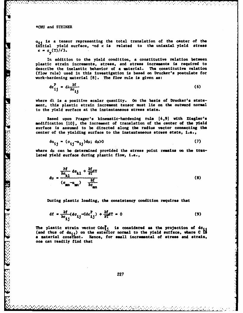
*CHU and STEINER
* 4 Is a tensor representing the total translation of the center of theinItial yield surface, -nd K is related to the unlaxial yield stressK- y(T)/3.
In addition to the yield condition, a constitutive relation between.:. plastic strain increments, stress, and stress incrments is required to
describe the inelastic behavior of a material. The constitutive relation(flow rule) used in this investigation is based on Drucker's postulate forwork-hardening material [8). The flow rule is given as:
de P d (6)
where dX is a positive scalar quantity. On the basis of Drucker's state-ment, this plastic strain increment tensor must lie on the outward normalto the yield surface at the instantaneous stress state.
Based upon Prager's kinematic-hardening rule [4,91 with Ziegler'smodification [10], the increment of translation of the center of the yieldsurface is assumed to be directed along the radius vector connecting thecenter of the yielding surface to the instantaneous stress state, i.e.,
daij - (o i-ij)du; dp>O (7)
where dp can be determined provided the stress point remains on the tran-lated yield surface during plastic flow, i.e.,
af30k' dal 3T
iidu k (8)
amn
During plastic loading, the consistency condition requires that
df - ft o-Cdc~ )+ JT - 0 (9)aaU (ij Ii
The plastic strain vector Cdejj is considered as the projection of do 4
(and thus of del ) on the exterior normal to the yield surface, where C IJa material cons nt. Hence, for small Incremental of stress and strain,one can readily find that
227
,.1
-- .c .,., ," .,' ," " , ", '-," ' '-.'. '. '..- '- '-.'-.' .- . - -.- ..', , '.:',.-,,-'.-" ...' " ." :,.'. ;'- . '. '.. . .' . ., • .,.. .

*CHUJ and STEINER
af + fJ
dX 01 (10)
Therefore, the flow rule becauses
af
de~ + z(- (11)Ij C(a3 Of qk k a
an a
If axisymmetric deformation is considered, with reference to thecylindrical coordinates (r, 0, z) the state is def ined. by the nonvanishing
stress components (do)T _ < do doe, doz, dTrz > and strain components*(delT _ < der de) dez, dyrz >- Then, the incremental stress-strain
relations are found In the following matrix form:
(do) (D[] (del - dT (B) (12)
In which,
1-V V V, 0 S2 S SS ST
v V -lv 0 8 2 SS S9T[II~ ~ -~-T1 z OrzV -V 0 95 5 2 St- (13)
z r z 0 z z rz
0 0 0 1-2v T S T S T S T 2
L rz r rz0 e z rz
1_ ( 11 f
A I T1v(-v (15)
228
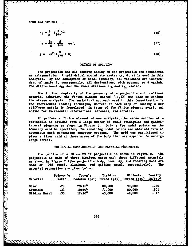
'2- *CU and STEINER1 (16)
" "i (A- .. )2 (16)
2 and, (17)g
.g 2i2.(K . + C) (18)
METHOD OF SOLUTION
The projectile and all loading acting on the projectile are consideredas axisyintric. A cylindrical coordinate system (r, 8, z) is used in thisanalysis. By the assumption of axial symmetry, all variables are indepen-dent of angle 8, consequently, all derivatives, with respect to 6 vanish.The displacement ug, and the shear stresses TrO and Tez vanish.
Due to the complexity of the geometry of a projectile and nonlinearmaterial behavior, the finite element method [11,121 was used to conductthe stress analysis. The analytical approach used in this investigation is
*the incremental loading technique, wherein at each step of loading a newstiffness matrix is formulated, in terms of the finite element model, andsolved for incremental deformations, stresses, and strains.
To perform a finite element stress analysis, -the cross section of aprojectile is divided into a large number of small triangular and quadri-lateral elements as shown in Figure 1. Only a few nodal points on theboundary need be specified, the remaining nodal points are obtained from an
Sautomatic mesh generating computer program. The grid was partitioned toplace a finer grid at those areas of the body that are expected to undergolarge stress.
PROJECTILE CONFIGURATION AND MATERIAL PROPERTIES
The outline of a 30 a XM TP projectile is shown in Figure 2. Theprojectile is made of three distinct parts with three different materialsas shown in Figure 2 (the projectile body, nose cap, and rotating band aremade of 1018 steel, aluminum, and gilding metal, respectively). Thematerial properties are given below:
Poisson's Young's Yielding Ultimate DensitTMaterial Ratio Modulus (psi) Stress (psi) Stress (psi) lb/in.
Steel .29 29x10 6 88,500 90,000 e280Aluminum .33 lOxl0 6 77,000 80,000 .101
J Gilding Metal .33 17x106 40,000 48,000 .317
229
4l
. . . . .. . . . . . . . . . . . . . . . . . . . .
*CHUJ and STEINER
The stress-strain relations of those materials are shown in Figure 3.
N 4
LO (D
(NFgrJ. rjcieCofgrtoC.-
W, 0
0 0 1"U,0(N (Nd I'0v .
AA GILIN META,-~WWWUU U~W
* S ~*~.01
0-230
*CHU and STEINER
LOADING CONDITIONS
The loads considered in this investigation simulating the environmentin the gun barrel during firing. The loading consisted of four types:(1) propellant gas pressure, (2) setback force due to acceleration, (3)rotational velocity due to the spin of projectile, and (4) forced displace-ment of the rotating band. The maximum value of these four types ofloadings are given by, Pmax - 60,000 psi, am. - 4.8x10 7 in./sec2 , %ax A6,335 rad/sec, and A. - -0.008 inches for gas pressure, acceleration,spin rate, and radial -displacement, respectively.The frictional shear forces betweenthe band and the barrel wereneglected in this investigation. , 00The loads were applied in incre- S &mental fashion with the relative ! 0smagnitudes at each load point _simulated the physical interde- 60pendence of the loads at differenttimes during the interior ballistic Wcycle. The detailed loading history 2
is given in Figure 4.
0 0 20 30 40 50 so 70
TIME STEP
Figure 4. Loading Hlstory
COMPUTATIONAL RESULTS
For each incremental loading, the stresses and strains of eachelement and the displacement of each nodal point were calculated. Theplastic flow has been initiated within element 186 of the gilding metal atthe end of the first step of loading. Based upon the Von Mises yieldcriteria, the equivalent stress for each element was calculated. At theend of the first step of loading, the maximum equivalent stres (a.) in
the projectile body is 69,900 psi which is lower than yielding strength of1018 steel (element 174), and in the gilding metal portion is 40,000 psi(element 186), which is equal to the yield strength of the gildingmaterial.
The computation results presented in this section are based upon thefollowing three major loading steps (shown in Figure 4):
L 231
r -': -.- -_., • ;, - -. " " - , .-. " '- • - . '" . " . -. .. -. -" '• . " - . ". .

*CHUJ and STEINER
1) At the end of the 12th step (4-1.0, p-0.5, a-0.5, and w2 -O.036)while the forced displacement reeaches the maximum in the rotating band.
2) At the end of the 33rd step, (A-1.0, p-1.0, a-1.0, and w~0.4while both propellant gas pressure and setback force reach the peak.
3) At the end of the 63rd step (A-1.0, p-0, a-0, and w .)while the spin rate reaches the maximum at the muzzle end of the tube.
The plastic range in the projectile under the above three loadingconditions is shown In Figure 5, 6, and 7, as indicated by the shadedarea.
@1 0
*0U C) V* .- 4
%404 0 .-
4 .01
2322
*CHU and STEINER
The maximum plastic strains encounteredIo in the gilding metal (element 186) is
00 0.027 In./in., and in the projectile is
04 0.025 In./in. (element 163) at the endSof the 12th loading step, while the max-
imum radial displacement took place in0 the rotating band. The maximum plastic.0 strains were increased to 0.0294 In./in., C o (element 186) in the gilding metal and0. 4-4 to 0.0254 in./in. (element 163) in theU. 0 a projectile body, while both gas pressure
Soand setback force reached the peak.:o:. cc When projectile reached the muzzle end
P4 the maximum plastic strains are 0.0294__ _ .in./in. and 0.0258 in./in, encountered
in the elements 186 and 163, respective-4 JT/,2 ly. During the entire loading process
$. the change of maximum plastic strain is '?0. '-small. The location of plastic zones
" 14 under different loading conditions is
important to the projectile design.
The equivalent stress along thelength of the inner surface elementsof the projectile is shown in Figure8. The maximum equivalent stressreaches 88,800 psi, which Is greaterthan the yielding strength (a .
88,500 psi) and smaller than the ..ultimate strength (ou - 90,000 psi) y ::'1...... -of the projectile material. If theinvestigation was based on elastic 7,analysis, the maximm equivalentstress could reach a value whichwould be much higher than the ulti- ~mmate strength of the projectilematerial., This is the reason thatour inelastic analysis technique bedeveloped, since a more rigorous .JA.- '-.-'': stress analysis can only be obtained .. SONC ALON ,.M1§ ,.ELE,. ME.NTS . ..
by using nonlinear theories of plas-ticity as developed in this See Next Page for Enlarged Scale- investiation.ivs.a n Figure 8. Equivalent Stress in the
Inner Elements of the Projectile.
233
ra-.
, .,, :,,. 3 ._. ., -. .-.- ,..-., .. .,..,-..-. ... - . ._ ..... ,-.. . .-
,. . . . .. . . , .
*CHUl and STEINER
0 0
. .
03 cv
* 0 z
ob so o0 t m m
.1-ww mm"
VAv~-
*CHU and STEINER
The equivalent stress distribu- 0tion in the projectile of high stres-sed region at peak pressure and set-back Is shown in Figure 9. It i W 0clearly indicated that the critical " ,region is located from the rotating " C Nband to the inside wall of projectile .- 44 V aI.4rdO 3
base. t
4i 0
The deformed grids under diffe-rent loading conditions are shown in C 4 0Figures 10, 11, and 12. The deforma- 4 . 0
:3.9 4 dtions shown in these Figures are the
deformations enlarged 10 times in ri0 00magnitude. '" - -. _
$- , 4 A
1-44. Qt 0 0 .a
"on"
4.4
0 0
-' U0
A .: .--
0 t
00
235

*CHU and STEINER
_-', := CONCLUSIONS
-- On the basis of Drucker's flow rule
0- C; ,of plasticity, the Von Mises flow. 1 criterion, and the strain-hardening
and compressibility properties of a.... material, a more rational rigorous
nonlinear elastoplastic analytic
method has been develped for anal-yzing and designing a projectilesubjected to actual complicated0 0
44 - f firing conditions. In constrast to0 -H the traditional designing and
• analyzing techniques (theories ofelasticity), the complex phenomenal
00 0 plastic flow in the projectile has;s- a been taken into account.
This is due to the necessity of designing for maximum stress to achieve anoptimal design for reducing component weight. Both nonlinear materialresponse and geometric nonlinearity have been taken into consideration.Nonlinearity of material properties has taken into account by use theoriesof platicity. Geometric nonlinearly has been considered by use the finiteelement technique. An incremental loading procedure has been used toconsider the actual firing environment of a gun. The complete loadinghistory which includes propellant gas pressure, setback force, and spinrate of a projectile was defined as function of time.
The critical region is located in the region between rotating bandand projectile base. In this region the equivalent stress in general isabove the yield strength of material, however, it is below ultimatestrength of the material. The plastic strain has taken place in thereigon, however, maximum equivalent plastic-strain at inner surface isbelow 0.03 in./in., which is relatively small.
Based upon our investigation the plastic zone in the projectile hasbeen identified and accurately located for each incremental of loadingwhich simulating the actual fire environment in a gun. The developed
-.technique will provide a more rigorous stress analysis tool for projectiledesign. The potential design flaws and critical regions of a projectilecan be identified before the projo-tile is being made and tested.
236
. . . . . . . . . ..-
*CHU and STEINER
REFERENCES
1. DePhillipo, T.E., and Booth, A.W., "Mathematical Model forDetermining Stresses in Projectile Bodies," Report R-1939, FrankfordArsenal, Oct 1969.
2. Mechanical Engineering Department, New York University,"Principal and Combined Sresses of the Shell, HE 155 m M197," PicatinnyArsenal Report U38115.
3. Elder, A.S., Burns, B.P., and Hurban, J.M., "Stress Analysis of175 m Projectile, HE 4437, BRL Memorandum Report 2113.
4. Prager, W., "The Theory of Plasticity: A Survey of RecentAchievement (Hames Clayton Lecture)," Proc. Inst. Mech. Eng. 69 (1955).
5. Prager, W., "Nonisothermal Plastic Deformation," Proc. Koni, Ned.Akad., Van Weton, Series B, 61, NO (3), 1958.
6. Chu, S.C., "Nonisothermal Elastoplastic Deformation of Work-Hardening Solids," Paper presented at Joint ASME/ASCE MechanicsConference, University of Colorado, 22-24 June 1981.
7. Chu, S.C., "An Incremental Appraoch to Nonisothermal Elastic-Flastic Deformation." Proc. 27th Conference of Army Mathematicians, 1981.
8. Drucker, D.C., "A More Fundamental Approach to Plastic Stress-Strain Relations," Proc. 1st U.S. National Congress Applied Mechanics, NewYork, 1952.
9. Prager, W., "A New Method of Analyzing Stresses and Strains inWork-Hardening Plastic Solids," Journal App. Mech. Vol. 23, 1956.
10. Ziegler, H., "A Modification of Prager's Hardening Rule,"Quarterly of App1. Math Vol. 17, 1959.
11. Zienkiewicz, O.C., "The Finite Element Method in EngineeringScience." McGraw-Hill, 1971.
12. Marcal, P.V. and King, I.P., "Elastic-Plastic Analysis of Two-Dimensional Stress Systems by the Finite Element Method," Inter. J. Koch.,Vol. 9, No. 3, 1967.
237
..........- * ~ - ~ . . .. .
CORN & PENA
MUNITION EXPENDITURE MODEL VERIFICATION:KIXK PHASE I (U)
*STEPHEN L. COHNRICARDO PENA
US ARMY ATMOSPHERIC SCIENCES LABORATORYWHITE SANDS MISSILE RANGE, NEW MEXICO 88002
The threat imposed by the Soviet bloc tank forces requires thatground level obscuration, for both offensive and defensive planning, mustreceive the most thorough research and developmental efforts. The possl-bility of reducing costs for munition expenditures further dictates pur-suit of more efficient mechanisms for obtaining obscuration objectives.
A large data base from previous experiments exists in the litera-ture, covering chemically generated military smokes. These data havebeen used to verify and/or evaluate several different approaches to atmo-spheric diffusion, including the Gaussian formulae. These previous testshave verified the predictability of relatively long average downwindconcentrations of some diffusing materials In the atmosphere. However, adeficiency exists in the case of military smokes for which the actualobscuration has not been reliably predicted or verified, especially overshort time Intervals. This deficiency has made it impossible to evaluateKWIK, a munition expenditure model, in all categories of performancewithout obtaining additionaJ data.
In order to verify the munition expenditure predictions of the KWIKmodel, an evaluation plan consisting of three phases was devised byAtmospheric Sciences Laboratory (ASL). This paper deals only with PhaseI, an effectiveness evaluation test for visible wavelengths.
1. DESCRIPTION OF MODEL
The [WIK (a mnemonic derived from crosswind Integrated concentra-tion) model consists of a blending of meteorological and site parameters,atmospheric optics, and turbulent diffusion theory. Each of these arebriefly discussed below.
239
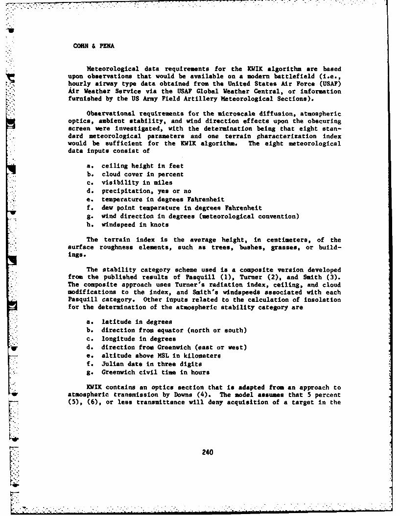
COHN & PENA
Meteorological data requirements for the KWIK algorithm are basedupon observations that would be available on a modern battlefield (i.e.,hourly airway type data obtained from the United States Air Force (US"F)
AIr Weather Service via the USAF Global Weather Central, or informationfurnished by the US Army Field Artillery Meteorological Sections).
Observational requirements for the microscale diffusion, atmosphericoptics, ambient stability, and wind direction effects upon the obscuringscreen were investigated, with the determination being that eight stan-dard meteorological parameters and one terrain characterization indexwould be sufficient for the KWIK algorithm. The eight meteorologicaldata inputs consist of
a. ceiling height in feetb. cloud cover in percent
c. visibility in milesd. precipitation, yes or noe. temperature in degrees Fahrenheitf. dew point temperature in degrees Fahrenheitg. wind direction in degrees (meteorological convention)h. windspeed in knots
The terrain index is the average height, in centimeters, of the* :surface roughness elements, such as trees, bushes, grasses, or build-
ings.
The stability category scheme used is a composite version developedfrom the published results of Pasquill (1), Turner (2), and Smith (3).The composite approach uses Turner's radiation index, ceiling, and cloudmodifications to the index, and Smith's windspeeds associated with eachPasquill category. Other inputs related to the calculation of insolationfor the determination of the atmospheric stability category are
a. latitude in degreesb. direction from equator (north or south)
c. longitude in degreesd. direction from Greenwich (east or west)e. altitude above MSL in kilometersf. Julian date in three digitsg. Greenwich civil time in hours
KWIK contains an optics section that is adapted from an approach toatmospheric transmission by Downs (4). The model assumes that 5 percent(5), (6), or less transmittance will deny acquisition of a target in the
240
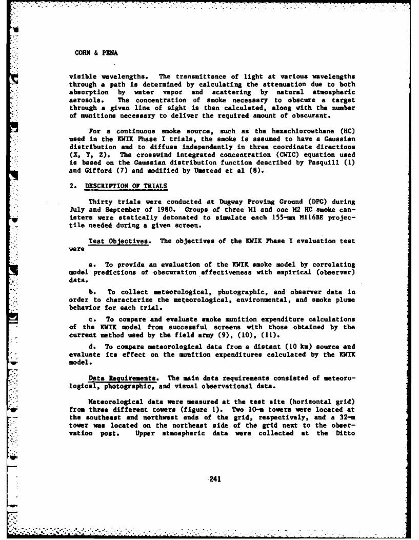
. . . .
COHN & PENA
visible wavelengths. The transmittance of light at various wavelengthsthrough a path is determined by calculating the attenuation due to bothabsorption by water vapor and scattering by natural atmosphericaerosols. The concentration of smoke necessary to obscure a targetthrough a given line of sight is then calculated, along with the numberof munitions necessary to deliver the required amount of obscurant.
For a continuous smoke source, such as the hexachloroethane (HC)used in the KWIK Phase I trials, the smoke is assumed to have a Gaussiandistribution and to diffuse independently in three coordinate directions(X, Y, Z). The crosswind integrated concentration (CWIC) equation usedis based on the Gaussian distribution function described by Pasquill (1)and Gifford (7) and modified by Umstead et al (8).
2. DESCRIPTION OF TRIALS
Thirty trials were conducted at Dugway Proving Ground (DPG) during
July and September of 1980. Groups of three MI and one M2 HC smoke can-isters were statically detonated to simulate each 155-mn M116BE projec-tile needed during a given screen.
Test Objectives. The objectives of the KWIK Phase I evaluation testwere
a. To provide an evaluation of the KWIK smoke model by correlatingmodel predictions of obscuration effectiveness with empirical (observer)data.
b. To collect meteorological, photographic, and observer data inorder to characterize the meteorological, environmental, and smoke plumebehavior for each trial.
c. To compare and evaluate smoke munition expenditure calculationsof the KICUK model from successful screens with those obtained by the
current method used by the field army (9), (10), (11).
d. To compare meteorological data from a distant (10 kin) source andevaluate its effect on the munition expenditures calculated by the KVIKmodel.
Data Requirements. The main data requirements consisted of meteoro-logical, photographic, and visual observational data.
Meteorological data were measured at the test site (horizontal grid)from three different towers (figure 1). Two 10-i towers were located atthe southeast and northwest ends of the grid, respectively, and a 32-Mtower was located on the northeast side of the grid next to the obser-vation post. Upper atmospheric data were collected at the Ditto
I ' '241
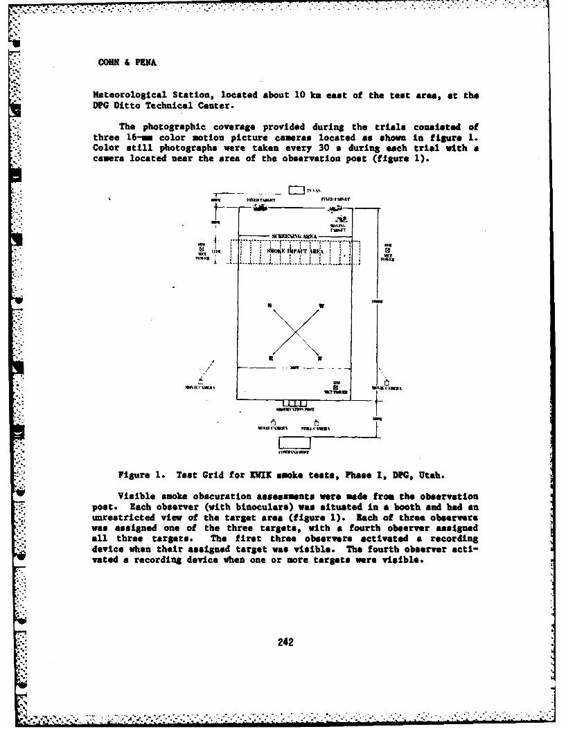
. . . . . . . . . . . . . . . . .. .. . . . . .
COHN &PENA
Meteorological Station, located about 10 km east of the test area, at theDPG Ditto Technical Center.
The photographic coverage provided during the trials consisted ofthree 16-rn color motion picture cameras located as shown In figure 1.Color still photographs were taken every 30 a during each trial with acamera located near the area of the observation post (figure 1).
W39FEINGE AREA
9 ! i - I , 1 s
1mW
n WN
lim"T imu
Figure 1. Test Grid for KUIK smoke tests, Phase 1, DPG, Utah.
Visible smoke obscuration assessments were made from the observationpost. Each observer (with binoculars) was situated In a booth and had anunrestricted view of the target area (figure I). Each of three observerswas assigned one of the three targets, with a fourth observer assignedall three targets. The first three observers activated a recordingdevice when their assigned target was visible. The fourth observer acti-vated a recording device when one or more targets were visible.
242
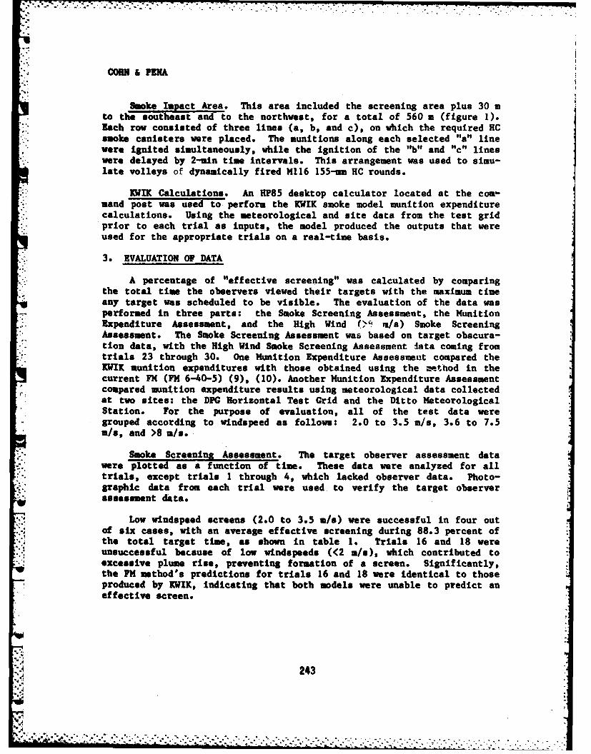
. COHN & PEA
Smoke Imact Area. This area included the screening area plus 30 mto the southeast and to the northwest, for a total of 560 a (figure 1).Each row consisted of three lines (a, b, and c), on which the required HCsmoke canisters were placed. The munitions along each selected "a" linewere ignited simultaneously, while the ignition of the "b" and "c" lineswere delayed by 2-min time intervals. This arrangement was used to simu-late volleys of dynamically fired M116 155-m HC rounds.
: IK Calculations. An HP85 desktop calculator located at the com-
mand post was used to perform the KWIK smoke model munition expenditurecalculations. Using the meteorological and site data from the test gridprior to each trial as inputs, the model produced the outputs that wereused for the appropriate trials on a real-time basis.
3. EVALUATION OF DATA
A percentage of "effective screening" was calculated by comparingthe total time the observers viewed their targets with the maximum timeany target was scheduled to be visible. The evaluation of the data wasperformed in three parts: the Smoke Screening Assessment, the MunitionExpenditure Assessment, and the High Wind (>9 /s) Smoke ScreeningAssessment. The Smoke Screening Assessment was based on target obscura-tion data, with the High Wind Smoke Screening Assessment lata coming from
* -"trials 23 through 30. One Munition Expenditure Assessment compared theKWIK munition expenditures with those obtained using the method in thecurrent FM ( M 6-40-5) (9), (10). Another Munition Expenditure Assessment
,.7 compared munition expenditure results using meteorological data collectedat two sites: the DPC Horizontal Test Grid and the Ditto MeteorologicalStation. For the purpose of evaluation, all of the test data weregrouped according to windspeed as follows: 2.0 to 3.5 m/s, 3.6 to 7.5u/s, and >8 m/s.
Smoke Screening Assessment. The target observer assessment datawere plotted as a function of time. These data were analyzed for alltrials, except trials 1 through 4, which lacked observer data. Photo-graphic data from each trial were used to verify the target observerassessment data.
Low windspeed screens (2.0 to 3.5 m/s) were successful in four outof six cases, with an average effective screening during 88.3 percent ofthe total target time, as shown in table 1. Trials 16 and 18 wereunsuccessful because of low windspeeds (<2 m/s), which contributed toexcessive plume rise, preventing formation of a screen. Significantly,the FM method's predictions for trials 16 and 18 were identical to thoseproduced by KWIK, indicating that both models were unable to predict aneffective screen.
243
...............
......................- . . . . . . . . , . .
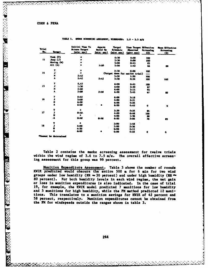
COHN & PENA
TANS 1. U SCUMNNG ASSESUW, SIsPZm: 2.0 - 3.5 S/
Initial Tim To Appr t Target Tim Target affective Eam affectiveTrial Screen Target guild Up Schedule O0eervd Screeni ng Screeming10. Target (ASS see) (min: oft) (mint eac) ("aam) (.) W
Task T) *4:30 0:00 10011 Jeep (J) 2:30 0:00 100
Nevif (N) 5 :00 0:45 a5All (A) * 1:00 5:00 1:42 44 88
T 2:30 0:00 10014 J * (Target dom for entire trial) -
N 2:42 5:30 1:50 100A 2:42 2:42 5:30 0:54 10 100
T 0.45 4:00 0:45 100IS J 1:30 6s0 3:30 67
N 2:00 6t00 2:15 93A 2:00 2:00 6:00 3:45 67 12
T 0:42 6:00 3:1616 J 5:00 4100 2:21
N 6:00 6:00 4:24A 6: 600 4:45 0 0
T 2:30 0:24 417 J 0:48. 4:00 0:48 100N 5:00 1:36 GA 0:48 0:48 6:00 2:04 78 83T 0 2:00 1:488 4:00 5:00 2:36N 4:30 6:00 2:12A 6:00 6:00 4:11 0
OCAiNt Ie deterUined
Table 2 contains the smoke screening assessment for twelve trialswithin the wind regime of 3.6 to 7.5 m/s. The overall effective screen-ing assessment for this group was 99 percent.
Munition Expnditure Assessment. Table 3 shows the number of rounds1KWIK predicted would obscure the entire 500 m for 6 min for two wind
groups under low humidity (RH -z30 percent) and under high humidity (RR-80 percent). For both humidity levels in each wind regime, the net gainor loss in munition expenditures is also indicated. In the case of trial19, for example, the 1CWIK model predicted 7 munitions for low humidityand 5 munitions for high humidity, while the FM method predicted 12 muni-tions. This translates to a munition savings for 1(1lK of 42 percent and
: 158 percent, respectively. Munition expenditures cannot be obtained fromthe PH for windspeeds outside the ranges shwn in table 3.
244
........ .... .....,:..".."..,-..............................
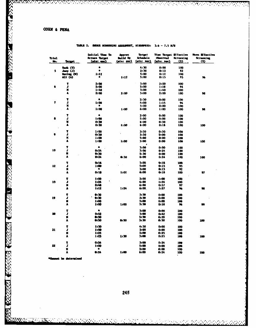
9,,
COHN & PUIA
TAMAS 2. SUt SCIESING *SSESPOt VIU EPUFD: 3.6 - 7.5 K/S
Initial Tim. To Approm T rst Tim Tarset Uftective Kom MfectlveTrial Screm Target Build Up Schedule Observed Screenmg Screening
b. Target (stag am) (*l: ee) (mt: aee) (Stu: sec) (Z) (Z)
ThA (T) 4:30 0:00 1005 Jeep (J) 2:30 0:12 92
Iving (1) 1:12 5:00 0:12 100All (A) 6 1:12 5:00 0:15 95 96
T 2:00 3:00 2:00 1004 J 2:00 5:00 1:18 94
- 1:40 3:00 1:40 100A 2:00 2:00 5:00 2:00 100 98
T a 2:30 0:00 1001:00 4:00 1:15 94
18 * 5:00 0:00 100A 1t: 1:00 6:00 1:00 1000 96
T 2:00 0:00 100-. J 1:00 5:00 0:00 100
-. 0:30 :00 0:30 100A 0:30 1:00 6:00 0:18 100 100
T 1300 3:30 0:30 100J 0:30 3:30 0:00 100
I 1o0 5:00 0:00 100A 1:00 1:0 5:00 0:00 100 100
T * 3:00 0:00 10010 J 0:24 3:00 0:24 100
M, 0:30 5:30 0:00 100A 0124 0:30 6:00 0:O4 100 100
T 1g StOQ o:11 1o12 1 1:00 5:00 0:15 95
* 0 3:00 0:15 92
A 0:3I 1:00 6;00 0:18 00 97
T 1:00 3:00 1:00 10013 3 1:24 6:00 1:24 100
N 0:40 6:00 0:57 97A 1:12 1:24 6:00 1:27 9 96
T 0:20 3:30 0:00 10019 J 0:30 3:30 0:00 100
N 1:00 5:00 0:00 100A I:0 1:00 5:30 0:18 9 %9
T *3:00 0:00 1oo20 3 0:42 3:00 0:42 100
N 0m:3 5:30 0:20 100A 0:50 0:30 5:30 0:50 100 100
4 1:30 4:30 0:00 10021 1 100 3:00 0:00 100
K 1125 5:00 0:25 100A 1:25 1:30 5:00 0:25 100 i00
T 0:24 3:00 0:24 10022 J 1:00 5:00 0:00 1001 * 3:00 0:00 100
, A 0124 1:00 6:00 0:24 100 100
7.: semot be datefale
245
. . . . - ...... -. " .I .. ... ... . ... ..... .. ... i i . ... i " "+•' I ... . :+ + ++ I+
"" ",-' '"... .,"'" "" ... ""+:,I"""" '9-.-. ''
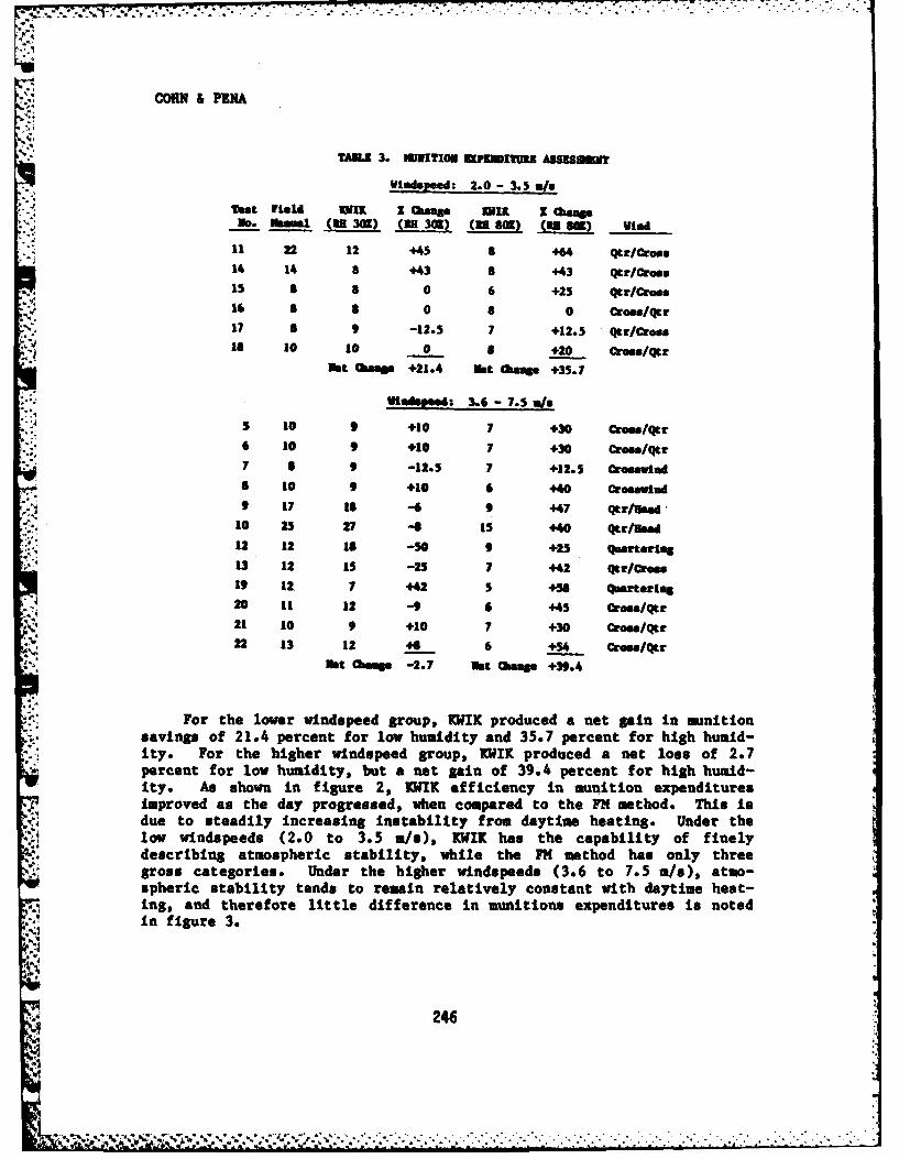
COiN & PENA
S TANA 3. IhIITIOU IXPlKi I ASSESSMIT
VindSpeed: 2.0 - 3.5 n/1
Test Field 11K= Z mawnge 3 Z (aege-. Naomi (U30() (M30() (338(3) (n $a) Vied
11 22 12 +45 8 +64 Qtr/Cro14 14 a +43 + +43 qtr/Croe.is a 8 0 6 +25 tr/Cous16 8 8 0 8 0 cro/Qcr17 9 9 -12.5 7 +12.5 tr/cro1 10 10 0 8 +20 Cros/Q1r
Mst a +21.4 Est OMWe +35.7
V- lpeedi 3.6 - 7.5 u/n
" 5 10 9 +10 7 +30 Croas/Qtr6 10 9 +10 7 +30 cros/qtr7 6 9 -12.5 7 +12.5 Cron"ie da 10 9 +10 6 +40 Crosuwlad9 17 18 -6 9 47 Qtr ad
10 25 27 -8 15 440 qtr/Usad; 12 12 18 -50 9 +25 quartering
13 12 15 -25 7 42 Qtr/Croee
19 12 7 442 5 +58 Qurtering20 11 12 -9 6 445 Cross/qtr
21 10 9 +10 7 +30 Crom/Qtr22 13 12 44 6 +54 Crom/tr
Net enge -2.7 Nt 0avas +39.4
For the lover windspeed group, KUIK produced a net gain in munitionsavings of 21.4 percent for low humidity and 35.7 percent for high humid-ity. For the higher windspeed group, KIK produced a net loss of 2.7percent for low humidity, but a net gain of 39.4 percent for high humid-ity. As shown in figure 2, KUIK efficiency in munition expendituresimproved as the day progressed, when compared to the FM method. This isdue to steadily increasing instability from daytime heating. Under thelow windspeeds (2.0 to 3.5 m/s), KUIK has the capability of finely
. describing atmospheric stability, while the I1M method has only threegross categories. Under the higher windspeeds (3.6 to 7.5 m/s), atmo-spheric stability tends to remain relatively constant with daytime heat-in$, and therefore little difference in munitions expenditures is notedin figure 3.
246
- 5 %*~.;3v%~* -2" -' *-* *.: . - .*W- V
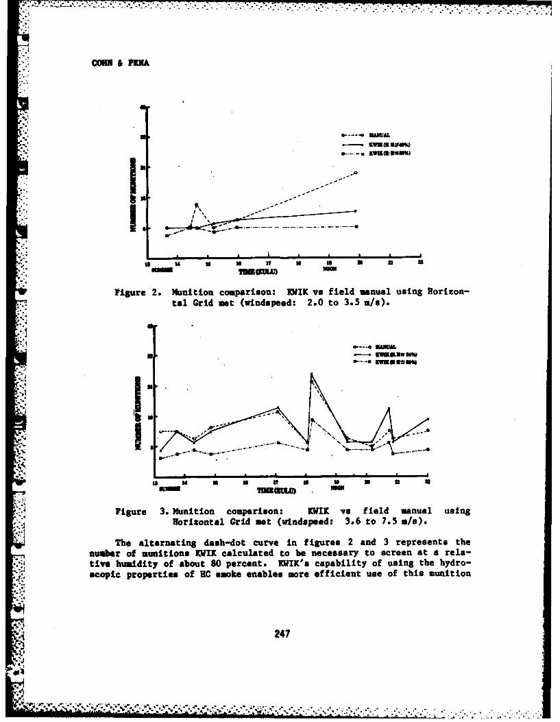
- coosn& PENA
'" o-----o MANUAL
I n
I ~ A. 16 -------- i*--------
3 1 Id 35 3 I V U7 10 tf 1 3
Figure 2. Munition comparison: 11IK vs field manual using Horizon-
tal Grid met (windspeed: 2.0 to 3.5 a/s).
,~I
-Figure 3. Munition comparison: KIK vs field manue l using
Horizontal Grid mt (vindspeed: 3.6 to 7.5 m/s).
The alternating dash-dot curve in figures 2 and 3 represents the
number of munitions KI1 calculated to be necessary to screen at a rela-
tive humidity of about 80 percent. KWIl's capability of using the hydro-
scopic properties of HC smoke enables more efficient use of this munition
247
V: . , -, . - . . ,. . - - . . . ... . . . . . -... . . . - . . . ..I i5.|l mIl lih 'h hhiih~ d '~'bibi
'"' " -,"" " , ,", ,,,,, -.. "":. - '''.'
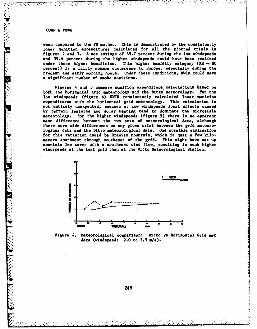
COHN & PENA
when compared to the FM method. This is demonstrated by the consistentlylower munition expenditures calculated for all the plotted trials Infigures 2 and 3. A net savings of 35.7 percent during the low windspeedsand 39.4 percent during the higher windspeeds could have been realizedunder these higher humidities. This higher humidity category (RH - 80percent) is a fairly common occurrence in Europe, especially during thepredawn and early morning hours. Under these conditions, KWIK could savea significant number of smoke munitions.
Figures 4 and 5 compare munition expenditure calculations based onboth the horizontal grid meteorology and the Ditto' meteorology. For thelow windspeeds (figure 4) KWIK consistently calculated lower munitionexpenditures with the horizontal grid meteorology. This calculation isnot entirely unexpected, because at low windspeeds local effects causedby terrain features and solar heating tend to dominate the aicroscalemeteorology. For the higher windspeeds (figure 5) there is no apparentmean difference between the two sets of meteorological data, althoughthere were wide differences on any given trial between the grid meteoro-logical data and the Ditto meteorological data. One possible explanationfor this variation could be Granite Mountain, which is just a few kilo-meters southwest through southeast of the grid. This might have set upmountain lee waves with a southeast wind flow, resulting in much higherwindspeeds at the test grid than at the Ditto Meteorological Station.
--- --- - ----- e-- --
2I: 1 IS il I? U I3 a aI *
Figure 4. Meteorological comparison: Ditto vs Horizontal Grid met
data (windspeed: 2.0 to 3.5 m/s).
248
. -.. . . . . . -. .
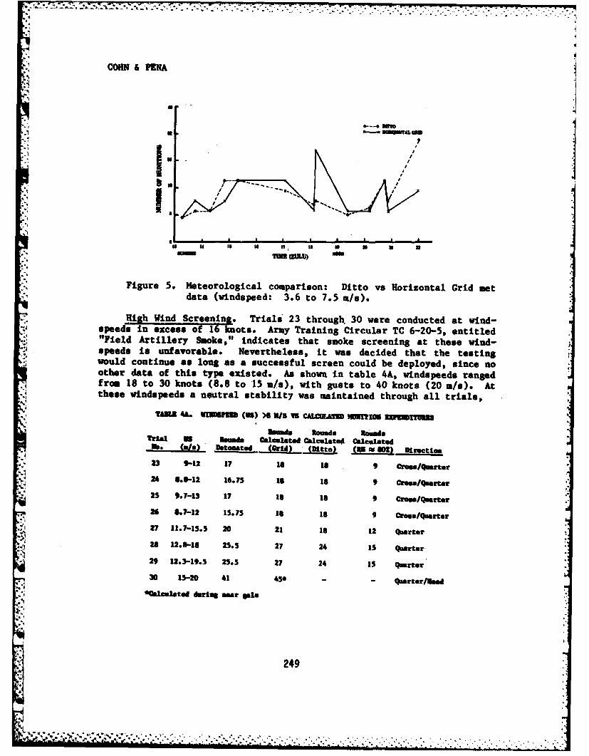
COHN L PENA
LGM
AA-4
Figure 5. Meteorological comparison: Ditto vs Horizontal Grid metdata (windspeed: 3.6 to 7.5 mas).
High Wind Screening. Trial.' 23 through. 30 were conducted at wind-speeds in excess of 16 knots. Army Training Circular TC 6-20-5, entitled"Field Artillery Smoke," indicates that smoke screening at these wind-speeds is unfavorable. Nevertheless, it was decided that the testingwould continue as long as a successful screen could be deployed, since noother data of this type existed. As shown in table 4A, windspeeds rangedfrom 18 to 30 knots (8.8 to 15 m/s), with gusts to 40 knots (20 m/s). Atthese windspeeds a neutral stabilit7 was maintained through all trials,
TAM 41. VSIWD (IS) >) U/S VS CMXhA= MIINION Xm1TU338
ends Rounds RoundsTrial n Rounds caleLated Calculateo CalelLatedno. W) Detomated L") (Dtto) (RE w 02) Direction
23 9-12 17 1 15 9 Cram/Quarter
24 8.3-12 16.75 1s 18 9 CroMP/Quarter25 9.7-13 17 Is 18 9 Cro"uaarter
26 5.7-12 15.75 Is is 9 Croes/Quartor
27 11.7-15.5 20 21 1 12 Quarter238 12.8-18 25.5 27 24 15 Quarter
29 12.3-19.5 25.5 27 24 15 Quarter30 15-20 41 45* - - qasrterSud
*ftleulated devise sear sale
249
V.4 ,';'.',.-, ;..- ,.. . - . . . .-.. , . ... . . . . . . . .
*44 . .. ... ' . . -" . . ' - -" " -"" " , "" " " ' , . "
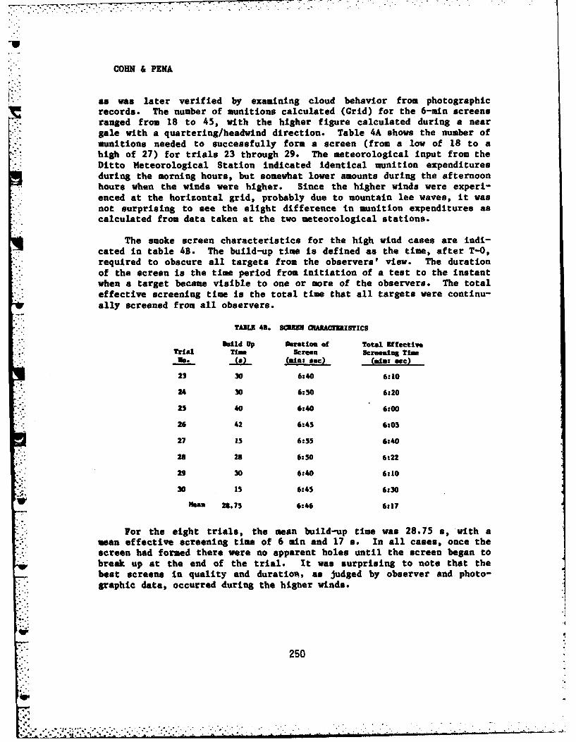
COHN & PENA
as was later verified by examining cloud behavior from photographicrecords. The number of munitions calculated (Grid) for the 6-min screensranged from 18 to 45, with the higher figure calculated during a neargale with a quartering/headwind direction. Table 4A shows the number ofmunitions needed to successfully form a screen (from a low of 18 to ahigh of 27) for trials 23 through 29. The meteorological input from theDitto Meteorological Station indicated identical munition expendituresduring the morning hours, but somewhat lower amounts during the afternoonhours when the winds were higher. Since the higher winds were experi-enced at the horizontal grid, probably due to mountain lee waves, it wasnot surprising to see the slight difference in munition expenditures ascalculated from data taken at the two meteorological stations.
The smoke screen characteristics for the high wind cases are indi-cated in table 4B. The build-up time is defined as the time, after T-O,required to obscure all targets from the observers' view. The durationof the screen is the time period from initiation of a test to the instantwhen a target became visible to one or more of the observers. The totaleffective screening time is the total time that all targets were continu-ally screened from all observers.
TABLE 43. SCUN CRARACTIEISTICS
Bald Up Duration of Total IffeetieTrial TIMs Sere.e Screening Tim
no.( (ads: sc) (Ulu: see)
23 30 6:40 6:10
24 30 6:50 6:20
25 40 6:40 6:00
26 42 6.45 6:03
27 15 6:55 6:40
28 28 6:50 6:22
29 30 6:40 6:10
30 15 6:45 6:30
Nsan 28.75 6:46 6:17
For the eight trials, the mean build-up time was 28.75 s, with amean effective screening time of 6 min and 17 s. In all cases, once thescreen had formed there were no apparent holes until the screen began tobreak up at the end of the trial. It was surprising to note that thebest screens in quality and duratioA, as judged by observer and photo-graphic data, occurred during the higher winds.
250
o-
S S'', .Ti ,' _ . S'' .. ........ . "..... . . . . . . . . . . . .-. . . . ..'- . ..-." ' ' '
'
COHN & PENA
The similarity of the munition expenditure calculations from boththe Ditto Meteorological Station and the horizontal grid met stationwould seem to indicate that under certain synoptic scale events, thetarget meteorology is similar to the meteorology several kilometersaway. These types of large scale weather systems are not unusual inEurope, especially during the winter months. Another common featureduring the winter storms is high relative humidity (RH -80 percent).Results using such a high relative humidity are indicated in table 4A.All other meteorological parameters are identical. A reduction in muni-tions of 47.39 percent over the cases with lower humidities illustratesthe wide variation possible under varying ambient moisture conditions.This variation is important, considering that the FM method does not havethe capability to screen under high winds nor to use the ambient moistureto reduce expenditures under high humidities.
4. CONCLUSIONS
Screening Effectiveness. In this initial phase of testing, K'WIK hasdemonstrated that it not only is more efficient in munition utilizationthan the FM method, but that it also has the capability to calculatemunition expenditures under meteorological conditions that the present FMmethod considers impractical. For the low windspeed or marginal screen-ing category (2.0 to 3.5 m/s), two trials were unsuccessful in forming ascreen because of low windspeeds and extreme variability of wind direc-tion. Since calculations for these same two trials using the FM methodproduced identical munition expenditures, both techniques failed to suc-cessfully screen under these meteorological conditions. The remainingfour trials in the low wind category produced a mean effective smokescreen during 88.3 percent of the screen duration time. The fewinstances during which a target was visible were almost always caused bysignificant changes in windepeed and wind direction during the course ofa trial.
There were twelve trials conducted under favorable screening condi-tions, with windspeeds ranging from 3.6 to 7.5 m/s. These trials pro-duced a 99-percent mean effective screen. All of these screens wouldhave denied acquisition of a target for the duration of the screen.
Munition Expenditure Comparisons. Phase I was conducted under dryconditions, with an average relative humidity of only 30.5 percent.These dry conditions are important, because HC is a hydroscopic smokewhose screen capabilities are greatly enhanced under the higher humidi-ties that are frequently found in Europe. For the marginal screening
V category, KWIK used 21.4 percent fewer munitions than the FM method.However, under high humidities (RH - 80 percent), KWIK could have saved35.7 percent of the rounds that the FM method required for the same mis-sions.
251
*~ ~ ~~ ~ ~~ ~~~ .......... .* ... - ,
. * . . . * . . . * .
COHN & PENA
In the favorable screening category KWIK used 2.7 percent more muni-tions than the FM method required. However, under high humidities (RH*80 percent), KWIK would have produced a 39.4 percent savings in muni-tions expenditures. The failure to incorporate the relative humidityeffects into the FM method clearly causes an excess expenditure of smokerounds under the higher humidity conditions.
Target Area Meteorology. Under marginal screening conditions, thewinds are variable in both space and time. Even under the relativelyuniform terrain of DPG, use of the target area *eteorology produced asavings in munition expenditures, as shown in figure 4. As windspeedsincrease, local wind circulations disperse and the general flow becomesmore uniform. During the transition period between low and high wind-speeds, tremendous variability can exist over a spatial distance of only10 km (figure 5). In the wintertime European scenario, major stormscovering hundreds of kilometers are quite common. Many of these stormsare associated with windspeeds high enough to preclude the necessity ofknowing target area meteorology to perform a mission. (This assumes thatthe terrain features do not dominate the target area meteorology.) Underweaker wind regimes, which occur in Europe during the summer season,local wind circulations would make the availability of target area meteo-rology desirable or even necessary for the completion of a mission.
High Wind Screening. One of the surprises of Phase I testing wasthe discovery that it is practical to screen a target during highwinds. Eight trials were conducted under high wind (8.0 to 15.0 m/s) or"unfavorable" screening conditions, with a 100-percent mean effectivescreen. All these screens obscuzed all targets for more than therequired 6 min, as seen in table 4B.
There are several possible reasons for the successful screening athigh windspeeds. One plausible explanation is that the vegetationflattens as the windspeed increases, lowering the effective roughnesslength. This lowering of the roughness length would change the disper-sion parameters, which are critical to the correct calculation of muni-tion expenditures. Examining table 4A, it is noted that the actual num-ber of munitions that successfully detonated was always less than the
* number calculated. Since all of the screens were successful, this over-prediction of needed munitions could be due to wind-modified roughnesslength. Another possibility is the homogeneity of the terrain at DPG.
- It is possible that for heterogeneous terrain or terrain with extensivevegetation, such as a forest, the increased turbulence at higher wind-speeds would preclude the use of smoke. A third possibility is a changein the efficiency of continuous burning smoke munitions during highwinds. An increase in the oxygen available to the munition could con-ceivably improve the efficiency of such munitions.
252
COHN & PENA
Regardless of the reason or combination of reasons for the high windsmoke screening, further investigation is clearly warranted. If futureexperiments confirm that smoke screening at high windspeeds is feasible,then a change in doctrine would be indicated. This could give friendlyforces an advantage in future confrontations using smoke.
6. REFERENCES
1. Pasquill, F., Atmospheric Diffusion, 2nd edition Halsted Press, divi-
sion of John Wiley & Sons, Inc., New York, 429 pp, 1974.
2. Turner, D. B., "A Diffusion Model for an Urban Area," J ApplMeteorol, 3:83, 1964.
3. Smith, F. B., "A Scheme for Estimating the Vertical Dispersion of aPlume from a Source Near Ground-Level," unpublished Meteorological Officenote, 1973.
*.4. Downs, A. R., A Review of Atmospheric Transmission Information in theOptical and Microwave Spectral Regions, Report 2710, US Army BallisticResearch Laboratory, Aberdeen Proving Ground, MD, 1976.
5. Gordon, Jacqueline I., Daytime Visibility, A Conceptual Review,AFGL-TR-79-0257, Visibility Laboratory, Scripps Institute of Oceanog-raphy, La Jolla, CA, 1979.
6. Schuppert, G. T., "Visibility Concepts and Measurement Techniques forAviation Purposes," DOT-TSC-FAA-71-25, Transportation Systems Center,Cambridge, HA, 1971.
7. Gifford, F. A., "An Outline of Theories of Diffusion in the LowerLayers of the Atmosphere," Meteorology and Atomic Energy, D. Slade,editor, US Atomic Energy Commission, Washington, DC, 1968.
8. Umstead, R. K., R. Pena, and F. V. Hansen, KWIK: An Algorithm forCalculating Munition Expenditures for Smoke Screening/Obscuration inTactical Situations, ASL-TR-0030, US Army Atmospheric SciencesLaboratory, White Sands Missile Range, NM, 1979.
9. JTCG/ME, "Summary Tables of Estimated Ammunition Expenditures toEstablish and Maintain Smoke Screens," unpublished manuscript.
10. Field Artillery Smoke, Training Circular 6-20-5, US Army FieldArtillery School, Fort Sill, OK, 1975.
11. Modern Battlefield Cannon Gunnery, Field Manual 6405, Headquarters,Department of the Army, Washington, DC.
K 253
...................- " - l "
COMMINGE
HARDENING OF ARMORED VEHICLESUSPENSION COMPONENTS
HUBERT COMMINGE, MR.US ARMY MOBILITY EQUIPMENT R&D COMMAND
FORT BELVOIR, VA 22060
INTRODUCTION
Mechanically-emplaced and air-delivered land mines have beenintroduced into the modern battlefield thus compounding the problem ofmaintaining armored-vehicle mobility. Land mines and mined areas will beencountered by U.S. Forces throughout the battlefield during offensive,defensive, and rear-area support operations. In tracked vehicles, thevulnerable components are those associated with the suspension system and,most particularly, the tracks and roadwheels. This is a critical problemarea; a small 3-pound explosive charge can cause a mobility failure onall tracked vehicles. The major damage resulting from such an explosionis the loss of a track section, resulting in an izmnobile vehicle. Sinceminefields are usually covered by artillery and anti-tank weapons, animmobilized vehicle can be destroyed quickly.
Historically, warfare scenarios and deployment techniques havelimited the use of land mines to certain well-defined situations toimpede or channel opposing forces. Advance knowledge of minefieldlocations could permit effective countermeasures using mine-clearingequipment such as mine-clearing rollers mounted on lead vehicles,projected explosive line charges, or, depending on mine density, bullingthrough with some sacrifice. The advent of offensive mining throughair- Pnd artillery-delivery capabilities has introduced a new tacticalsituation that requires mobile units to proceed across random-laid
*minefields or mine areas.
Vulnerability analysis has predicted severe losses of armored combatunits in all mine environments. This prompted investigations forproviding countermine hardened suspensions for armored vehicles. Thefollowing guidelines were developed for hardening tank track shoes androadwheels thus providing enhanced survivability:
. . . .. . .. . . . . ..
COMMINGE
a. Suspension components should be hardened to demonstrate enhancedblast survival from the explosion of a undirectional shallow-buried charge.
b. Hardened components should not exceed the weight of currentsuspensions.
c. The M60 tank tracks and roadwheels should be the baselinesuspension components.
d. The vehicle should be mobile after a single encounter and-: . should be able to "limp-off" the minefield and preclude a complete kill
(K-Kill).
SUSPENSION FAILURE ANALYSIS
Current tank track shoes and roadwheels are severely damaged whensubjected to an explosive charge, even a s11 (3-pound) track-cuttingexplosive charge. An analysis was conducted to determine the mode offailure in order to develop the protection mechanism.
In explosive charge-target geometries, where the explosive is indirect mechanical contact with the target, the predominant failuremechanism is shear caused by a large-velocity gradient. This can beillustrated qualitatively by Figure 1.
Target
Free Shear Failure- Surf ac e -4 / Plane
Figure 1. Arbitrary charge/target geometry.
In this arbitrary target, the explosive, simulating an air-scatterablemine, is in direct contact with the target. Detonation of this chargecauses a high-pressure shock wave to be propagated into the target materialadjacent to the charge. The interface between explosive and target movesupward at a high velocity. Material along the bottom edge of the target,not in direct contact with the explosive charge, receives no velocitywave and, therefore, remains initially at rest. This large velocity
I. o"
-.--. .. 2S6
%.
COMMI1GE
differential between material in contact with and material not in contactwith the charge, induces a strong shear stress in the target material.Since the compressive stress is essentially one-dimensional, a shearfailure is expected to propagate from the corners of the charge upward
.1 along the dashed lines. A similar mechanism also causes shear failure• , along the dashed lines emanating from the internal corner of the target'stop surface. The initial pressure-velocity wave propagates upward untilit reaches the free surface; at this time a rare-faction shock reflectsfrom the free surface and imparts a velocity which is approximately twicethat of the incident velocity. A velocity gradient exists between thematerial under the free surface and that where no free surface isencountered; therefore, a shear failure is expected.
Verification that a shear failure can occur around a discontinuityin a target structure is illustrated in Figure 2 below.
, 1
Figure 2. Dynamic X-ray of wheel deformation.
[ 257
V-'OS mA'O

-ft..CONNINCE
This doubly exposed radiograph shows a wheel section before and 450microseconds after initiation of an explosive charge. The wheel wasspecially constructed for this test and incorporated chosendiscontinuities. The wheel rim consisted of weldments of laminated bandsand alternating layers of steel and aluminum, with the outermost bandbeing aluminum. The explosive charge, as shown in the radiographexposure, was placed directly against the wheel to simulate anair-scatterable mine. A shear failure starting from the spoke-rim jointis clearly demonstrated in the 450-microsecond X-ray exposure.
Tests similar to that described above were coiducted with differenttank roadwheel and track-shoe configurations to locate critical failurepoints in component structures and to determine how these failures couldbe controlled or eliminated. Discontinuities within the mine-targetenviroment were the key to component failure. First, almost all observedfailures occurred around discontinuities resulting in large-velocitygradients between adjacent portions of material; second, discontinuitiesthat occurred in the structure without inducing a velocity gradient oftenhad the effect of inhibiting failure propagation. In addition, tests
- demonstrated that reduction of target surface area normal to the explosiveblast resulted in a proportional reduction in the overall load deliveredto the target structure.
From the roadwheel and track-shoe test results, the protectionrequirements for tank suspension system survival from landmines weredeveloped as follows:
a. Eliminate sharp geometric discontinuities.
b. Use laminatians to inhibit crack propagation.
c. Pre-plan fracture geometry to protect critical tank suspension
components.
d. Reduce normal area adjacent to the explosive charge.
e. Use energy-absorbing materials.
. f. Incorporate blast deflection in tank roadwheel and track design.
ROADUREEL AND TRACK DESIGN
The major disadvantages to the current tank roadwheel and track
shoe structure, when subjected to a track-cutting explosive charge,are the large flat surface areas presented to the explosive blast source;
258
i .': "i'"...'....'......i, . .. ..U ... [lumli / nn' "" "un l- --- -.. . .
COIINGE
in addition, the components contain sharp geometric discontinuities. Thelarge area absorbs the full brunt of the explosive blast and is notconducive to dissipating or deflecting the shock wave. Further, themetal components trasmit the large-velocity gradient to other suspensioncomponents such as roadarms and torsion bars and cause additional damage.
The new suspension configuration encompasses a single tank roadwheelIn lieu of the present dual-roadwheel system and a track shoe having asemi-circular groove for maintaining proper track alignment and interfacewith the roadwheel. This single roadwheel allows a large amount of theexplosive blast to flow by and dissipate quickly; hence decreasing/eliminating the damage to the roadwheel and other suspension components
2 * such as the roadarm, shock absorbers, and torsion bars.
The hardened roadwheel internal structure consists of sevenfiberglass radial support rings with an outer ring encapsulated in anelastomeric material as shown in Figure 3.
.4:
... . ....
t*F:BE LASS- ' ......... STRUCTURE "
, w • ELASTOMERIC
Figure 3. Hine-resistant tank roadwheel. '
259 ,
.4-4
COMMINGE
The support rings are fabricated of E-glass tape bonded with EPON 828epoxy and Z-modified polyamine; the cure procedure consists of hardeningat room temperature and 4 hours at 2750 F. The encapsulant is AdipreneAPR-882 polyurethane and MOCA-cured.
The mode of deformation for the roadwheel structure under load froman explosive blast occurs initially at the single point of tangency betweenthe outer rim and one of the inner rings. As the explosive blast load isapplied, both rim and inner ring deform so that the area of mutual contactincreases continuously. Since rim-ring contact area increasescontinuously during loading, structural discontinuity does not occur at asingle point and the large-velocity gradient is spread over a wider areaminimizing and/or eliminating structural damage depending upon explosivecharge size.
The hardened track shoe was developed to provide the requiredstructual integrity, proper floatation, and minimum area of primarystructure adjacent to the explosive blast. The shoe consists of twometallic links with accommodating pins and bushings, a metallic yoke, anda non-metallic track-shoe body as shown in Figure 4.
, a
Figure 4. Mine-resistant tank track shoe.
260D. ."...
; * a t %h'. . . . . . .-. . . . . . . . . . . . . . . . . . . . . . . . . .
COMKINCE
The links, yoke, and pins manufactured of 4340 steel and hardened toa Rockwell C43 provide necessary structural integrity for both mobilityand explosive blast and are configured to minimize the area of primarystructure. The primary purpose of the yoke, besides adding to thestructural integrity of the track shoe, is to eliminate the latitudinalseparation of the track links under explosive blast. Earlier testing ofhardened track shoes without yokes resulted in the breaking of largenumbers of non-metallic track-shoe bodies because of excessivelongitudinal and latitudinal motions of the track when subjected to anexplosive blast. The track-shoe body consisting of Adiprene L-315 (ShoreD-70) molded to the yoke, provides the necessary vehicle floatation andtraction and is sacrificed during the explosive blast; this loss allowsfor quicker dissipation and/or venting of the shock wave. The track-shoedesign is such that the links are inserted sideways into the opening ofthe yoke and rotated 90 degrees to lock in place; this design eliminatesthe currently used track-shoe end connectors and accessories. Further,the center guides are completely eliminated; track guidance is achieved bythe semi-circular groove of the track shoe body that allows better wheeltraversing for terrain contour.
ENERGY ABSORBING MATERIALS
Detonation of a landmine releases a large quantity of energy in avery short period of time, creating a large moment of inertia on the trackand roadwheel subsystem. Prior to destruction, the roadwheel Imparts amoment to the roadarm assembly which is transmitted to the torsion bar,causing catastrophic failure of these components. In addition, a largeantitank mine containing 15 pounds or more of explosive will remove thetorsion bar housing from the tank hull. Materials, other than metals,capable of absorbing some of the explosive energy were required todecrease the overall transmitted inertia and decrease suspension component
. destruction.
Different energy-absorbing materials were analyzed; the mostpromising material compositions were subjected to explosive blast tests.It was obvious that full-scale explosive testing of all promisingenergy-absorbing materials and design configurations would be prohibitive;therefore, a low-cost testing procedure was developed to eliminateundesirable composite materials. The testing was accomplished byfastening the energy-absorbing material to a rigid I-beam with one endpinned to a concrete foundation (as shown in Figure 5). The beam was freeto rotate about its pin joint, and rotation was measured by means of amechanical scribe. Beam mass and moment of inertia were determined priorto each test so that energy collected by the composite material sampleand transmitted to the beam could be calculated from measured beam
F261
V1CO)MINGE
rotation. A baseline material was required to compare the energydissipated or absorbed by each composite material sample; steel was chosenas the baseline material, with the assumption that it would not absorband transmit the energy directly to the beam.
Figure 5. Energy absorption test set-up.
The table gives a partial listing of composite materials tested f orthe tank track shoe. The vehicle must be capable of traveling after amine detonation; therefore, the composite material should dissipate 100percent of the energy to eliminate damage to other suspension componentsand yet remain intact to allow for vehicle floatation. For this reason,the composite materials having the highest percentage value of energy
* dissipated with the least damage were employed in full-scale testing ona combat tank.
262
-o
. . . . . . . . ... . .. .
,3*.
COMMINGE
Results of Energy Tests of Track Composite Materials
ENERGYMATERIAL DISSIPATED DESC ItTION OF() BLAST DAMAGE
Epoxy-Epon 828/Catalyst Y 60 Partially fragmentedUrethane-Uralite 3121S 18 Minimal
Z Epoxy-Epon.828/Catalyst Y, 53 Partially fragmentedSilica-Reinforced
Epoxy-Epon 828/Catalyst Y, 58 FragmentedS Steel-Reinforced
: Non Rigid Epoxy-Epon 61 Fragmented282/DDSA
Polyster-Glass-Reinforced 54 PulverizedEpoxy-25Z Keular- inch 64 Partially fragmented
High-Density Polyethylene 64 Eroded": Polycarbonate--Unfilled 59 MinimalE Polycarbonate--40% Glass Fibers 63 Fragmented
Polyurethane--40% Glass Fibers 59 Partially fragmented
Steel 0 Totally Destroyed
EXPLOSIVE TESTS
Both the present dual-roadwheel tank suspension and single-roadwheelhardened suspension systems were subjected to numerous full-scaleexplosive tests. Tests were conducted with operational and simulatedlandmines containing 5, 13, and 22 pounds of explosive. Most foreignlandmines contain cast TNT; therefore, all simulated explosive chargeswere fabricated with TNT.
The 5 pound explosive charge, simulating an air-scatterable mine,was placed in direct contact with the tank track as would occur in anoperational situation. The present dual-roadwheel suspension systemsustained the following major damage, causing a mobility kill:
a. Dual roadwheel completely demolished, whether steel or aluminum.
b. Two track shoes completely destroyed.
c. Broken torsion bar at the first station.
d. Broken adjusting link at roadarm connection.
263
................ ...... --. m-
. . . . .. . . . . .. . . , . . - .i " .. " "
COMMINGE
* The damage sustained by the hardened suspension from the sameexplosive charge was negligible, clearly demonstrating the energyabsorption of the chosen materials. As a matter of fact, the tankcontinued its mobility mission without degradation. The damage was:
a. Loss of two or three track shoe plastic bodies (designed to besacrificed during explosion).
b. Very slight cracking/peeling of roadwheel encapsulant.
The next phase of testing was conducted to determine damage fromoff-the-shelf antitank mines. The explosive charge contained 12.6 poundsof cast TNT and was encased to simulate typical Warsaw Pact landmines.The simulated mines were covered with 2 inches of soil. The dual-roadwheelsuspension consisted of steel roadwheels and T-142 track. The damagefrom the explosive blast is shown in Figure 6.
Figure 6. Damage to present suspension system from 12.6 pounds of TNT.
The damage, as shown above, was extensive and resulted in amobility kill as follows:
a. Complete destruction of three track shoes.
b. Complete removal of the first dual roadwheel from the spindle(the wheels were sufficien- '-amaged to prohibit reuse).
264
r .-.- .. .i
COHINGE
c. Broken torsion bar at the first station.
d. Broken adjusting link.
e. Loosening of first and second stations torsion-bar housingcaused by hull mounting-bolt shear.
f. Removal of roadarm from housing and rotating forward of vehicle.
The following damage to the hardened suspension (Figure 7) was muchless severe and did not result in a mobility kill:
a. Cracking of the roadwheel encapsulant.* b. Loss of three track-shoe plastic bodies (designed to be
sacrificed during explosion).
c. Loosening of adjusting link.
d. Loosening of first-station torsion-bar housing.
Loosening of the idler-wheel adjusting link eliminated the track tension,but since the track links remained undamaged, the vehicle was able to
• .proceed under its own power with mobility degradation.
ih
Figure 7. Damage to hardened suspension system from 12.6 pounds of TNT.
265
. .i
. ... .. . .. .
COM14INGE
The final phaae of testing was conducted using 22 pounds ofexplosive; this equates to the largest off-the-shelf antitank mines. T'-apresent dual-roadwheel suspension system was not tested because thedamages would have been greater than previously encountered with the
* smaller explosive charges. The hardened suspension suffered a largeamount of damage, but not sufficient to cause a mobility kill. The dgewas as follows:
a. Roadwheel encapsulant is seriously damaged and inner ringstructure is slightly cracked.
b. Loss of 6 to 8 track-shoe plastic bodies.
c. Loosening of adjusting link.
d. Breakage of 3 to 4 track-shoe steel yokes.
e. Loosening of both the roadarm and torsion-bar housing causedby shear of mounting bolts.
Mobility was greatly reduced, but the vehicle still proceeded under itsown power. The track metal links and pins were not damaged and couldengage the tank drive sprocket.
CONCLUSION
The goal of the hardening program was to demonstrate that damagesto tank suspension systems from the detonation of a landmine could beminimized and, thus, decrease mobility kills. Through redesign andjudicious material selection, a new suspension concept was developedand demonstrated successfully, thus eliminating armored vehicle mobilitykills and allowing the vehicle to continue its intended mission or to berepaired for the next battle.
266
•................ . . .. ..0
-. 4-
COST* AND ALBRITTON
RESPONSE OF MX HORIZONTAL SHELTER MODELSTO STATIC AND DYNAMIC LOADING (U)
VAN T. COST, MR.* AND CAYLE E. ALBRITTON, MR.U. S. Army Engineer Waterways Experiment Station
Vicksburg, Mississippi 39180
INTRODUCTION
A concept considered for basing the Missile X System was to emplacethe missile in a buried, horizontal shelter. In support of the MX Hori-zontal Shelter Component Test Program, the U. S. Army Engineer WaterwaysExperiment Station (WES) developed and performed a program of static anddynamic model tests so that response data on specific structural detailsand shelter components could be obtained. The objectives of the test pro-
*- gram were to evaluate the load capacity merits of various shelter soil-structure design concepts and to optimize certain parameters, while pro-viding a design team with timely data necessary for structure survivabil-ity verification and construction economy comparisons. Static load vs.damage data from such tests provide necessary input for dynamic analyses,
- while dynamic test data help verify those analyses and the applicabilityof static data in predicting dynamic response.
The test articles were all 1/7.25-scale models of a cylindrical con-crete shelter segment, which were assembled with thrust-restraining hard-ware and buried horizontally in a soil material simulating that found in atypical siting area. The first phase of the program consisted of static
*- . tests on 17 cylinder models having a number of design parameters including.**backfill stiffness, depth of burial, reinforcement type, liner thickness,
shear stud spacing, and wall thickness, as well as the modeling of suchconstruction details as breakout joint sections and inspection panels. Inthe course of these initial tests, designs of the shelter system were de-veloping and being modified in response to test data and other factors.Upon completion of the initial 17 tests comprising Phase I, a specificstructure design was adopted. A likely combination of cylinder wallthickness, backfill stiffness, and removable panel detail was chosen asthe baseline for a second phase of eight static tests, in which the re-sponses of this baseline design and certain -variations thereof were ex-amined. The baseline model structure was also tested dynamically to ver-ify the similarity of static and dynamic response modes. The response of
267
COST* AND ALBRITTON
each model was monitored with electronic instrumentation.
This paper discusses the Phase II static tests and the associated dy-namic verification tests, and summarizes their results. Conclusions con-cerning the relative merits of the selected wall thickness, burial depth,backfill stiffness, and opening detail for the baseline shelter design arepresented.
DESCRIPTION OF TEST ARTICLES
All structures discussed herein were cylindrical concrete shells withsheet steel liners and welded shear studs. The cylinders had inside diam-eters of 24 inches and lengths of 48 inches. Outside diameters varied asprescribed by the wall thicknesses of 1.8, 2.4, 3.0, and 3.6 inches. Re-inforcement, other than steel liners and shear studs, consisted only of agrid of wire in the outer face which modeled the prototype's temperaturereinforcement. The baseline cylinder had a 3.0-inch wall thickness.
Most of the cylinder models included a removable panel in the crownsection which was a model of the required inspection panel opening. Thispanel consisted of matching Z-shaped metal frames with imbedment dowelswelded along the edges. Other construction details of the panel matchedthose of the adjacent structure section.
STATIC TEST PROCEDURES
All shelter model sections and appurtenant hardware were constructedat WES using materials conforming to invisioned prototype specifications.Reuseable concrete forms were machined from rolled steel for close toler-ances and i smooth concrete finish. A single inner form designed for dis-assembly trom within a cast cylinder was iied for all models, since insidediameters remained constant. One outer foim and one aligning baseplatewere built for each wall thickness of cylinder model to be tested, so thateach model of a given wall thickness could be cast in the same formassembly.
Construction of a cylinder model was begun with the fabrication of* the inspection panel frame. The frame was assembled with a steel liner,
shear studs, dowels, reinforcement, and appropriate instrumentation gagesand gage mounts, and wan mounted on a machined mandrel for casting (Fig-ure 1). The mandrel was attached to a vibration table during casting toassure concrete consolidation. Transparent acrylic rolled to the propercurvature was fastened to the panel to serve as outer formwork. After24 hours, the completed panel was removed from the mandrel and fastened tothe inner cylinder form, along with the steel liner and welded studs, ooterreinforcement, and instrumentation gage mounts (Figure 2). Outer form-work was then assembled (Figure 3), and the cylinder cast in a vertical
268
't J1
-1
."2..1
COST* AND ALBRITTON
* to
4$
0)
.,444
utu
P4 ~0a
4t'
71~
2690
COST* AND ALBRITTON
orientation. Concrete consolidation was accomplished using pencil vibra-tors carefully threaded into stud spacings marked along top flanges of theformwork.
After removal of formwork, a model cylinder was cleaned, instrumented,and assembled with the thrust-restraining hardware (Figure 4). This hard-ware consisted of 3-inch thick steel end plates and an internal thrustcolumn designed to carry all of the axial loads exerted by soil pressurenormal to the end plates. Rings of 1/2-inch-thick rubber were sandwichedbetween the model structure and each end plate to prevent the intrusion ofsoil without transferring significant axial load. These hardware werenot considered test articles.
A specially designed loading chamber approximately 6 feet in diameterwas used for the static tests. The steel test chamber was lined with2 layers of greased polyethylene to reduce the effects of sidewall fric-tion. Virgin soil was placed and compacted, for each test, to the eleva-tion of the cylinder invert, where a leveled strip of sifted soil was pre-pared for bedding the structure. After careful positioning, the backfillprocess was continued by hand in the areas near the cylinder invert, toassure uniformity. Backfill density and moisture content were systemati-cally monitored during backfilling using both sand cone and nuclear mea-suring device techniques (Figure 5). Two regions of soil were delineatedin the test chamber: an in-situ zone having stiffness characteristics ofthe undisturbed soil in a prototype siting area, and a backfill zone oflesser density representing excavated and recompacted soil. Figure 6illustrates the geometry of an assembled cylinder model and soil in thetest chamber.
Water pressure from a rate-controlled pump served as the loadingmedium in the static tests. Water pressure was sealed from the backfillsurface by a rubber membrane in a floating seal ring. The Central FiringStation (CFS) of the Blast Load Generator facility at WES was used as thereaction structure for the loading head-test chamber assembly (Figure 7).
Active electronic instrumentation in the static tests included straingages on liners and outer reinforcement and structure interface pressuregages at several locations around the cylinder, vertical and horizontaldiameter change gages, free-field soil stress gages, and loading pressuregages. Measurements were recorded on analog tape and later digitized forplotting. Remote-controlled in-structure cameras were also used to docu-
:" ment response in some tests.
DYNAMIC TEST PROCEDURES
Models constructed for dynamic tests were of the baseline design andwere identical to those tested statically. The four model cylinders were
270
COST* AND ALBRITTON
Figure 4. Assembly of thrust column and instrumentationfrom end of model.
Figure 5. Backfill density control around cylinder.
271
7- -77 7- 7 -
COST* AND ALBRITTON
FEW 0SAM AN" ~ ~ j A
T~~ MUNUm?~
igre .HrzotlclidrtstcnetLhas IIa tests
W'W'C*11U M
Urut" mM
Figure7. Tes chambr andoadin head inidCI'~@A reatio struturE
SI"IAV
272 rfiw
1................................................................ept-

COS= k AND ALERITTON
instrumented and assembled in the laboratory before being shipped to thetest site at the Fort Polk Military Reservation in Louisiana. Severaltruckloads of the simulated siting area soil used in the static tests weretransported from WES to Fort Polk for construction of the test beds. TheFOAM High-Explosive Simulation Technique (FOAM HEST) was used to simulatenuclear weapon overpressures.
For each dynamic test, native soil was excavated in an area 16 feetsquare to a depth of 8 feet, and was replaced with the simulated sitingarea soil. As in the static tests, soil placement densities were con-trolled as specified for both in-situ and backfill zones (Figure 8). TheFOAM HEST explosive charge was assembled over the entire backfill surface(Figure 9), and a sand overburden of appropriate thickness was placed overthe charge (Figure 10). Electronic instrumentation measurements includedall those made in static tests, as well as structure accelerations andairblast pressures at the backfill surface. Figure 11 illustrates thetest bed layout for the dynamic tests.
BASELINE MODEL DESIGN AND INVESTIGATED VARIATIONS
Ongoing shelter design during the first phase of the WES tests pro-duced the baseline for Phase II. The 1/7.25-scale model of the baselinedesign had a wall thickness of 3.0 inches and included an inspection panelspanning 75 degrees of the crown section over a length of 12 inches asshown in Figure 6. The inspection panel frame used 20 gage steel, and theliner material was 18 gage. Shear studs and outer reinforcing wire were0.086 inch in diameter, spaced at 1.65 inches each direction. Soil den-sities used for baseline design tests were 128 and 121 pounds per cubicfoot (pcf), dry density, for the in-situ and backfill zones, respectively.Depth of burial was 8.25 inches, measured over the crown.
The baseline configurations of the inspection panel, liner, studs,and reinforcement represented final designs and were not varied in thePhase II tests. However, one model with no inspection panel was tested todocument the panel's effects on response of the baseline design. Wallthickness effects were investigated in tests of three models other thanthe baseline with thicknesses ranging from 1.8 to 3.6 inches. One test
V incorporated a backfill density equivalent to the in-situ density to exam-ine backfill effects. Although the 8.25-inch depth of burial was notchanged in the Phase II tests, this was an investigated parameter sinceall of the Phase I tests were performed at depths of 3 or 6 inches, andmany of those structures were otherwise similar. All dynamic test config-urations were of the baseline design, and varied only in the environmentoverpressure and duration.
It is recognized that parametric investigations of only a single test
are not sufficient to accurately quantify the effects of such variables.
273
-. . • . •... .. . . .
* - COST* AND ALBRITTON
Ix
its1U HI
-4-
000
2744
COST* AND ALBRITTON
However, the primary objectives of the Phase II tests were to quantifystatic response of the baseline shelter design only, while identifying thetrends of influence certain variations might have. Three of the eightPhase II static tests were of the baseline concept.
RESULTS AND DISCUSSION
As with most structural testing programs, it was necessary to specifya criteria defining a particular level of damage or, at least, some pres-sure level at which a test would be terminated. Due to the functional re-quirements of the shelter and the extreme deformation capabilities of theload-carrying soil-structure system, it was decided that static testsshould be terminated prior to catastrophic failure. Since the operationof prototype missile transport systems and other hardware depended on cer-tain interior shelter features and clear spaces, "failure" of a modelstructure was defined as that overpressure at which disturbances of thesteel liner due to severe crushing of adjacent concrete occurred, i.e. theoccurrence or initiation of buckling of the liner. Instrumentation mea-surements and, in some cases, midtest photography were used to identifythe point during a test at which these criteria were met.
Response of the Baseline Design
The condition for the failure criteria was consistently met in thestatic baseline tests when severe concrete crushing occurred in areas justbelow cylinder springlines and buckles formed in the liners. Instrumenta-tion and photography indicated that these buckles formed suddenly (Figure12). The vertical diameter decrease due to ovaling deformation at thetime of liner buckling ranged from 1.0 to 1.6 inches (4.2% to 6.7%) in thethree baseline tests. The corresponding static overpressures ranged fromabout 350 to 600 psi. Comparisons of the three tests show that plots ofvertical diameter change vs. surface overpressure are quite consistent,and almost linear, with slopes of about 350 to 400 psi per inch of diame-ter change (Figure 13). Figure 14 shows a plot of horizontal diameter
- elongation vs. surface overpressure. Since springline buckles formed inthe areas of the deflection gage mounts in this test, their formation ap-peared as a disturbance on the plot, with an altered slope thereafter.
Although the response "stiffnesses" of the three baseline tests areconsistent, the points at which buckles occur during loading differ some-what with respect to diameter change and more severely with respect tosurface overpressure. It is suspected that slight differences in concretecompressive strenoths and local variations of backfill densities may havecontributed to the range of response magnitudes in which defined failuremechanisms initiated. Measured densities in the backfill areas of thethree baseline tests ranged from 119.3 to 122.6 pci, and concrete compres-sive strengths at test date ranged from 6580 to 7090 psi.
275
I III uiuimlublm...............................-...."...... ... ....
COST* AND ALBRITTON
04S.'4
UdT40 a
I.'
4.j
06
to8ow
276
* COST* AND ALBRITTON
4*1
c 7* 0'
'0 4
"4 44 : g
0004
44 $-46
0)
000 00 006 OOL O 00 £ 0 3 t 002 001
.44
U.277
.. . . . . . . . -
COST* AND ALBRITTON
Tests which were carried past the defined failure point showed thatspringline buckles continued to enlarge with additional cylinder ovalingand concrete crushing, and buckles also appeared as the invert hinge de-veloped. Shown in Figure 15 is an end view of a tested baseline modelhaving failure criteria damage, for which a residual vertical diameterchange of 1.3 inches was recorded. Shown in Figure 16 is a baseline modeltested beyond failure criteria to the point of invert hinge buckling.This model had a residual vertical diameter change of 2.1 inches.
Effects of Investigated Variables
Most of the Phase I shelter models were tested at a shallow 3-inchburial depth, and were less consistent in the type and location of failuremechanisms. Failures often occurred at the invert with loading curvesshowing slightly less response stiffness than those of similar Phase IItests. Shallow burial depths seemed to place tests near a breakpoint inresponse mode, as similar tests were sometimes observed to differ in de-formed shape and failure type.
Variation of wall thickness in the Phase II tests did not affect response mode (Figure 17). Models having thicker walls sho,-4 a trend to-ward slightly stiffer response. Failure overpressures of the wall thick-ness effects tests were all within the range of those for baseline tests,although ovaling was less severe at the time of failure for models havingthicker walls.
No significant response mode or failure point departures were experi-enced when the inspection panel was deleted nor when stiffness of soilbackfill was increased to that of the in situ. However, the structurewith no inspection panel did respond slightly stiffer than baselinemodels.
The explosive environments for the four dynamic baseline tests simu-lated weapon yields of approximately 0.5 to 1.0 kilotons, and ranged inpeak simulation overpressure from about 1000 to 3000 psi. In the mostsevere of these environments, structural damage was just reaching failurecriteria condition, with liner buckles visible just below springlines(Figure 18). This model had a residual vertical diameter change of
*1 2.0 inches.
CONCLUSIONS
1. The baseline cylinders responded statically in an ovaling mode" which caused failure mechanisms to occur at the springlines in the form of
* liner buckles due to severe crushing of concrete, followed by buckling atthe invert.
278
*W
7. 7. 777.
COST* AND ALBRITTON
Figure 15. Baseline model at failure criteria.
Figure 16. Baseline model loaded past failureto invert buckling.
279
'-.:
* COST* AND ALBRITTON
9y6
444
V.4
u0
P-1
5ao
94
80
AD-A128 Sl PROCEEDINGS OF THE 1982 ARMY SCIENCE CONFERENCE HELD RT 4/6THE UNITED STATES..(U) DEPUTY CHIEF OF STAFF FORRESEARCH DEVELOPMENT AND ACQUISITIG. 18 JUN 82
UNCLASSIFIED F/fl 5/2 N
mhEEmhohhooiIEEmhhhhohhhhhIEhhmhhmhEImEmsmhhhhhhhh~hhEhhEIEEEE-EEo
I .flllfflffllfllfllf
WL I" W rnIMU2O
U..0
I
MICROCOPY RESOWUTION TEST CHART NATIONA I Of STNOR-3A
NATIONA. BUREAU Om STANOAROS-1963-A
MICROCOPY RRESOLUITI TEST CHART
NATI- ONNATIN BURAU OF STANBU A-1U-A OF S-T---N--1 -A
.5.S 111"5
II
t/
112 -L, J~
~~~~~~~~~MICROCOPY RESOLUTION TEST CHART MCOOYRSL1rIi HR
NATIONAL ~ ~ ~ ~ ~ NAIOA 14M Of' STANDAU..M-19NTINL U0-AO 4*pIg M
.161
W-; 16.Lmi
.25. p
1"25, ,. m/" m"..... .- -. "'
.-01.6,
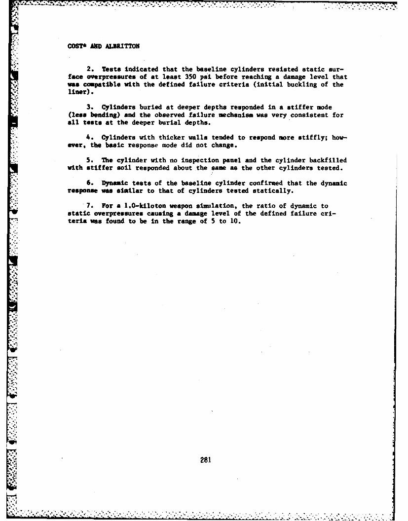
* .~ COST* AND ALBRITTON
2. Tests indicated that the baseline cylinders resisted static sur-face overpressures of at least 350 psi before reaching a damage level thatwas compatible with the defined failure criteria (initial buckling of theliner).
3. Cylinders buried at deeper depths responded in a stiffer mode(less bending) and the observed failure mechanism was very consistent forall tests at the deeper burial depths.
4. Cylinders with thicker walls tended to respond more stiffly; how-ever, the basic response mode did not change.
5. The cylinder with no inspection panel and the cylinder backfilledwith stiffer soil responded about the same as the other cylinders tested.
6. Dynamic tests of the baseline cylinder confirmed that the dynamicresponse was similar to that of cylinders tested statically.
7. For a 1.0-kiloton weapon simulation, the ratio of dynamic tostatic overpressures causing a damage level of the defined failure cri-teria was found to be in the range of 5 to 10.
28
*. . . . . . . ... .,. . . . . .
, . -'".. .
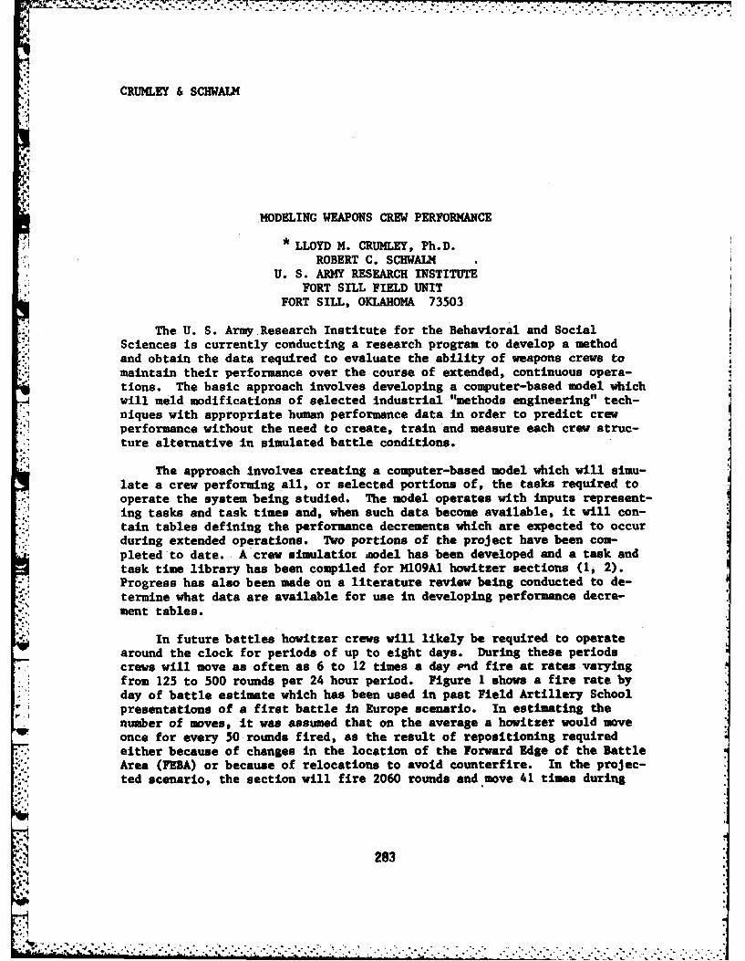
.. CRUMLEY & SCHWALM
MODELING WEAPONS CREW PERFORMANCE
* LLOYD M. CRUMLEY, Ph.D.
ROBERT C. SCHWALMU. S. ARMY RESEARCH INSTITUTE
FORT SILL FIELD UNITFORT SILL, OKLAHOMA 73503
The U. S. Army Research Institute for the Behavioral and SocialSciences is currently conducting a research program to develop a methodand obtain the data required to evaluate the ability of weapons crews tomaintain their performance over the course of extended, continuous opera-tions. The basic approach involves developing a computer-based model whichwill meld modifications of selected industrial "methods engineering" tech-niques with appropriate human performance data in order to predict crewperformance without the need to create, train and measure each crew struc-ture alternative in simulated battle conditions.
The approach involves creating a computer-based model which will simu-late a crew performing all, or selected portions of, the tasks required tooperate the system being studied. The model operates with inputs represent-
. ing tasks and task times and, when such data become available, it will con-tain tables defining the performance decrements which are expected to occurduring extended operations. Two portions of the project have been com-pleted to date. A crew simulatior model has been developed and a task andtask time library has been compiled for M109A1 howitzer sections (1, 2).
.7: Progress has also been made on a literature review being conducted to de-termine what data are available for use in developing performance decre-ment tables.
In future battles howitzer crews will likely be required to operatearound the clock for periods of up to eight days. During these periodscrews will move as often as 6 to 12 times a day nd fire at rates varyingfrom 125 to 500 rounds per 24 hour period. Figure 1 shows a fire rate byday of battle estimate which has been used in past Field Artillery Schoolpresentations of a first battle in Europe scenario. In estimating thenumber of moves, it was assumed that on the average a howitzer would moveonce for every 50 rounds fired, as the result of repositioning requiredeither because of changes in the location of the Forward Edge of the Battle
"*! Area (FEBA) or because of relocations to avoid counterfire. In the projec-ted scenario, the section will fire 2060 rounds and move 41 times during
283
I.
*1 '"' " '"" ' : :"'' i , '' -,:: ,r,;.",';:, ,:• ' '; " : - :'? -:' m ? ': ? '' :" ' " " :" ' - " ' ;:. '
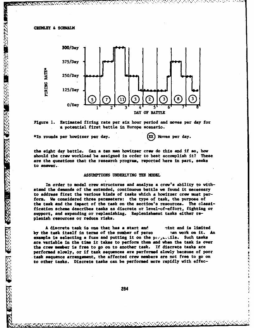
C1 E & SCHWAIM
300/Day,
375/Day
-pC
250/Day6
125/Day
7 810/Day 51 (D (
DAY OF BATTLE
Figure 1. Estimated firing rate per six hour period and moves per day fora potential first battle in Europe scenario.
*In rounds per howitzer per day. Moves per day.
the eight day battle. Can a ten man howitzer crew do this and if so, howshould the crew workload be assigned in order to best accomplish it? Theseare the questions that the research program, reported here In part, seeksto answer.
ASSUMPTIONS UNDERLYING THE MODEL
In order to model crew structures and analyze a crew's ability to with-stand the demands of the extended, continuous battle we found it necessary
to address first the various kinds of tasks which a howitzer crew must per-form. We considered three parameters: the type of task, the purpose ofthe task and the impact of the task on the section's resources. The classi-fication scheme describes tasks as discrete or level-of-effort, fighting orsupport, and expending or replenishing. Replenishment tasks either re-plenish resources or reduce risks.
A discrete task is one that has a start and sint and is limitedby the task itself in terms of the number of perso -an work on it. Anexample is selecting a fuze and putting it on the p-,.ile. Such tasksare variable in the time it takes to perform them and when the task is overthe crew member is free to go on to another task. If discrete tasks areperformed slowly, or if task sequences are performed slowly because of poortask sequence arrangement, the affected crew members are not free to go onto other tasks. Discrete tasks can be performed more rapidly with effec-
284I):,1 +' ++,.+ :+r+-+ +,+++ + ;% , ," i , ,'+ .+.. . ...+ ; . + . "+ . ,+ " + , + ".' .: :
CRUMLEY & SCHWALM
tive training and they lend themselves to rearrangement to improve thecrew effectiveness. Level-of-effort (LOE) is applied to all tasks whichare not considered as discrete. This category includes such activities asstanding guard, preparing defensive positions and sleeping.
The reason for the discrete vs level-of-effort task distinction is tosimplify the model. The tasks we have classified as discrete lend them-selves to analysis by the modeling approach we have adopted. Discrete taskscan be assigned in different orders and to different crew members; they canbe evaluated individually to determine the effects of various parameters,such as training or fatigue; and they are all involved in crew processes inwhich the quicker they are properly performed the better the crew performs.LOE tasks are a scheduling problem rather then a crew structure problem.LOE tasks tend to take longer to perform, do not lend themselves to a"quicker is better, so we should train to perform them faster" approach andusually have little or no room for being speeded up by a more effi-cientmethod.
In developing a rationale for our model we have also considered whichof two purposes a task serves. Fighting tasks include all those taskswhich must be performed when a howitzer section is emplaced, fired, ormarch-ordered (e.g., loading a projectile). Support tasks are all thetasks not classified as fighting tasks. Support tasks are performed inorder to maintain the ability of the section to continue to perform itsfighting tasks (e.g., amunition resupply).
Finally, tasks may be considered in terms of their impact on the sec-tion's resources. The fighting tasks all expend resources, e.g., firinguses amunition, moving uses fuel and men get tired. Support tasks, on theother hand, are intended to restore or conserve resources; hence, theyeither replenish resources expended as the section moves and fires, or theyreduce the risk that the section will be placed in a position where itsresources will be unnecessarily expended.
The task categories provide a basis for considering the tasks of ahowitzer crew in a series of steps rather than in a single stage. Thus, inmodeling a crew, and in actual operations, deciding if a crew can performadequately can be answered by determining first if they fight the howitzeradequately and then if they have time to perform the necessary supporttasks. Once this baseline has been established, performance during ex-tended, continuous operations can then be considered.
Three of the four cask sequences involved in fighting a howitzer--em-placement, firing, and march-order--are composed almost entirely of dis-
*. crete tasks. The fourth sequence, the in-transit phase, is composed mostly- of LOS tasks. It is feasible, therefore, to model the set-up, firing and
march-order sequences and evaluate how well different crew arrangements
285
#4lie
CRUMIJY & SCIWAL
meet time standards for performing these phases. This approach makes speedof performance a measure of a crew's ability to perform the task sequences
0involved in fighting the section. (Errors are taken into account by theirVI effects on speed. When errors are made, they must be corrected before pro-
ceeding, hence speed suffers.)
The number of persons not assigned to fighting duties determines theamount of time available for performing support functions. Judgments must
,0 be made concerning the priority of the various replenishment and risk re-duction tasks in order to assign the available personnel most efficiently.Now well a crew structure meets the support task requirements is then sea-sured by matching the support task man-hour requirements to the man-hoursthe crew structure provides to attend to them.
A crew structure is adequate when it meets the time standards forfighting task sequences and provides enough man-hours for the required sup-port tasks. Structures that do not fully meet these requirements becomeincreasingly inadequate as a function of both the lack of adequate supportma-hours and the additional time required to perform the fighting tasks.Selection between sub-optimal alternatives for actual operations is a pro-blem that requires the kinds of data that the Crew Performance Model canprovide.
The present standard crew operating procedure is defined in TechnicalManual 9-2350-217-10N (3). The procedure indicates that ten men emplace ahowitzer section, eight fire it, nine march-order it and either nine or tenmen are in-transit as the section moves between locations. This operatingprocedure provides little manpower for assignment to support duties. Forinstance, when the gun is firing, only two persons are available for sup-port duties. Thus, if a section were to remain n one location for an en-tire day, 48 an-hours (2 X 24) would be available for support duties.Since four hours sleep per man each day is a minimal support function, 40of these 48 hours would be required just to provide the crew with minimalrest.
Table I is a list of support tasks classified as replenishment or riskreducing. The task times were obtained mostly from doctrine requirementsand Fl ld Artillery School documents. Table I shows that support require-mmts easily exceed 129 man-hours per day. Thus, the support tasks which
1mut be performed if a howitzer section is operated around the clock andaccording to doctrine will almost certainly exceed the ability of the crewto perform them. For that reason Section Chiefs continually face a seriesof trade-offs: They must first decide how many people can be removed fromthe figbhting tasks; they must then evaluate the situation and set priori-ties on the replenishment and risk reduction duties required to support the
section and batter ; finally they must schedule the available support man-[ power to perform the most essential support tasks.
p
286
,.. ,.-,. .,,: . :._,. .. ............................. _ , . •. . _ . ..
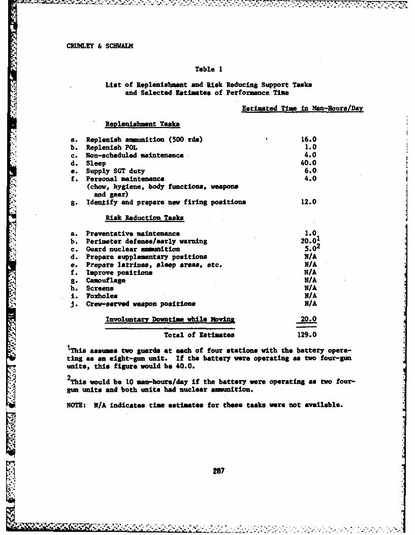
I.-I.- !k *J1
CRUNLEY & SCHWALM
Table 1
List of Replenishment and Risk Reducing Support Tasksand Selected Estimates of Performance Time
Estimated Time In Nan-Hours/Day
Replenishment Tasks
a. Replenish amuition (500 rds) 16.0b. Replenish POL 1.0c. Non-scheduled maintenance 4.0d. Sleep 40.0e. Supply SGT duty 6.0f. Personal maintenance 4.0
(chow, hygiene, body functions, weaponsand gear)
g. Identify and prepare new firing positions 12.0
Risk Reduction Tasks
a. Preventative maintenance 1.0b. Perimeter defense/early warning 20.01c. Guard nuclear ammunition 5.02
d. Prepare supplementary positions N/Ae. Prepare latrines, sleep areas, etc. N/Af. Improve positions N/Ag. Camouflage N/Ah. Screens N/Ai. Foxholes N/AJ. Crew-served weapon positions N/A
Involuntary Downtime while Ilovins 20.0
Total of Estimates 129.0
IThis assumes two guards at each of four stations with the battery opera-ting as an eight-gun unit. If the battery were operating as two four-gununits, this figure would be 40.0.2 This would be 10 man-hours/day if the battery were operating as two four-gun units and both units had nuclear ammunition.
NOTE: N/A indicates time estimates for these tasks were not available.
- ,.'. .......... .....
CRUNgMY & SCHWALM
STRUCTURE OF THE CREW PERFORMANCE MODEL
The ARI Crew Performance Model was developed to assist the SectionChief--or the system developer if the system is not yet fielded--in answer-ing such questions as how to structure a crew to deal effectively with bothfighting and support functions under a variety of conditions. The modelingapproach we use takes into account the tasks to be performed, the order ofperformance, the time it takes to perform each task, and the number of mendoing those tasks. The model consists of a task library, an input program,and the software to handle that information.
The task library contains the tasks and subtasks which must be perform-ed by the members of an M1O9A1 howitzer section. (A task library could bebuilt for any system, provided the discrete tasks making up that system canbe defined.) Each task is narrowly defined, has minimum, average, and maxi-mum completion times, and takes into account any requisite or concurrenttasks. Each library entry also has a task type code, a probability of per-formance value and an indication of how the time data were obtained. Theformat for task library entries is shown in Figure 2, Part A. Entries wereobtained from appropriate documentation, discussions with subject matterexperts and videotapes of two III Corps howitzer crews in operation. Forthe latter, each crew emplaced their section, fired three rounds and march-ordered; this cycle was performed four times. Thus, our times are generallybased on eight trials for emplacement and march-order tasks and 24 trialsfor firing tasks.
In order to use the model, the user-whether Section Chief or systemdeveloper--needs to specify the number of persons to which tasks will beassigned and then assign the tasks in the order each crew member will per-form them. An example of an input sequence is shown in Part B of Figure 2.The main program then simulates the number of iterations specified andprovides the output shown in Part C of Figure 2.
USING THE MODEL
The model has been used to determine the effects of various crew sizes/task assignments on the performance of howitzer sections. The base case isthe crew size/task structure as presented in the TH. For variations of
those structures, we deleted men and assigned their tasks to the remainingmen in such a way that those crewmen who were not very busy tended to as-sum most of the tasks, particularly those which were logically consistentwith their current positions. The results of several runs are shown inFigure 3. The figure shows completion times and percentages of crew mem-ber idle time for units of different sizes performing fighting task se-
quences. In the figure, completion time is expressed as a percentage of- the median time the model calculated for a full ten man crew performing thetask sequences according to the Technical Manual.
288
;.7- . . . . . . - - - -.
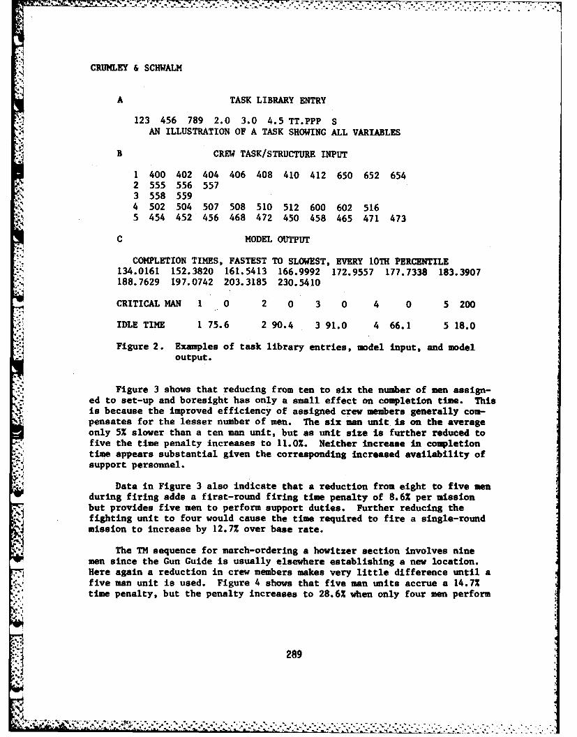
CRUMLEY &SCHWALM
A TASK LIBRARY ENTRY
123 456 789 2.0 3.0 4.5 TT.PPP SAN ILLUSTRATION OF A TASK SHOWING ALL VARIABLES
B CREW TASK/STRUCTURE INPUT
1 400 402 404 406 408 410 412 650 652 6542 555 556 5573 558 5594 502 504 507 508 510 512 600 602 5165 454 452 456 468 472 450 458 465 471 473
C MODEL OUTPUT
COMPLETION TIMES, FASTEST TO SLOWEST, EVERY 10TH PERCENTILE134.0161 152.3820 161.5413 166.9992 172.9557 177.7338 183.3907188.7629 197.0742 203.3185 230.5410
CRITICAL MAN 1 0 2 0 3 0 4 0 5 200
IDLE TIME 1 75.6 2 90.4 3 91.0 4 66.1 5 18.0
Figure 2. Examples of task library entries, model input, and modeloutput.
Figure 3 shows that reducing from ten to six the number of men assign-ed to set-up and boresight has only a small effect on completion time. Thisis because the improved efficiency of assigned crew members generally com-pensates for the lesser number of men. The six man unit is on the averageonly 5% slower than a ten man unit, but as unit size is further reduced tofive the time penalty increases to 11.0%. Neither increase in completiontime appears substantial given the corresponding increased availability ofsupport personnel.
Data in Figure 3 also indicate that a reduction from eight to five menduring firing adds a first-round firing time penalty of 8.6% per missionbut provides five men to perform support duties. Further reducing thefighting unit to four would cause the time required to fire a single-roundmission to increase by 12.7% over base rate.
The TM sequence for march-ordering a howitzer section involves ninemen since the Gun Guide is usually elsewhere establishing a new location.Here again a reduction in crew members makes very little difference until afive man unit is used. Figure 4 shows that five man units accrue a 14.7%time penalty, but the penalty increases to 28.6% when only four men perform
289
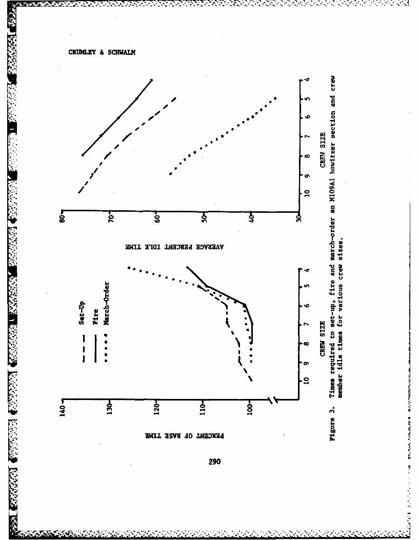
a.; CRIJMME SCHWALM
'Fa
-* %D U,-4e
- 0
0 AS40 4 441 0
10 -
tI *6 -A
/290
caEUwr SCWAWM
the march-order tesks. Thus, flourmom could be made availlable -for supportllutites without sipil icastly iuiaiLring perf ormac on D march-order tasks.
Prom thts analysis of crew structure of facts on set-up, firinS, andmarh-odertime, it appears tha4t Zitta tasks would not necessarily be
impaired vhea operating with a reded, Crew if the -crewm are more elf 1-clely assigned. ther, tasks. .3By dot"g this, not only Is Idle tim reducedbut persozsel are. treed to- performs necessary Support duties.
GOALS FOR WEAPONS CREW SRCUE
In considerIng the results of our simulation of howitzer crew opera-tions, we have forulated I i-e. goals m sa q mxaimed our data to deter-mine which crew structure befl at tit is The poals we 'think ust bemat by a adequate cre structure are:
1. * e able to Stpite, f ire, iarh-order and transferthde section Ina acceptable time or .t a aceptalie rate.
2. Permit enuhpeople to be assiguet to the support facetions thtatlack qf support does not reuethe section's fighting, ability to a Inade-quate, level.-
3.. gave a reasa$* capebility to reepaid4, in a degre4ed. wade, Vitasection personel are loet.
4. Ile effectively applied and pnacticed ina, peacetim milieu.5. Twinsts: to battle condtions ith # a~mtWel Mzda onthe craw.
VatA- ~ ~ to gf "eratl bth A-C "4a-imply that houitzercrws abb g*ificait Al led 60 -v a~b~flw~ baes for fi~gtimg
fioitei ecion r 4 Art sinwhich.6e. exdsting crewstructure antbecchenmre partia is to
divides tbe ten aa* crawia~it two via~a five~ ma mite (5/S).asttcrow tatalmuwpn 49 t *ts W~wit e fijaitgf amd
'A5/5spLfl t"tU is poodI* Tabl weeIttcoparedto the Cn#v as it 's4i~ il 4b , t eel baa.thecrwsut
wichA at* ideiaeal4*c titut o -e unit timiisSconO tadt"other :is supervised- by a hit 4Mtef.calmv aaainthese units ve4 0hteb! t i~tf ab~$ nvwf
tato u q tteL 1 sn nlsa ttme availablefor uprport tasteb ite a dvisia is ia log tab..
When a gun is apolae" aceordiag t eeg c .ativied ta the TM, thesatire tenM ilt c18 i 4 Slbth a ish Lwved. In t. 515 solua-
tion fie fria at u4ersad On0Mb(0 a) are Involved.Thmedia set-up timio q to* n $ 15 craw fea the standard
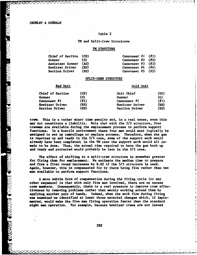
CRUMEY & SCHWALM
Table 2
TM and Split-Crew Structures
TM STRUCTURE
Chief of Section (CS) Cannoneer #1 (#1)Gunner (G) Cannoneer #2 (#2)Assistant Gunner (AG) Cannoneer #3 (#3)Howitzer Driver (HD) Cannoneer #4 (#4)Section Driver (SD) Cannoneer #5 (#5)
SPLIT-CREW STRUCTURE
Red Unit Gold Unit
Chief of Section (CS) Unit Chief (UC)Gunner (G) Gunner (G)Cannoneer #1 (#) Cannoneer #1 (#I)Howitzer Driver (HD) Howitzer Driver (HD)Section Driver (SD) Section Driver (SD)
crew. This is a rather minor time penalty and, in a real sense, even thismay not constitute a liability. Note that with the 5/5 structure, fourcrewman are available during the emplacement process to perform supportfunctions. In a hostile environment these four men would most logically beassigned to set up camouflage or emplace screens. Therefore, when the gunis reported up and ready in the 5/5 case, some of the support work wouldalready have been completed; in the TM case the support work would all re-
main to be done. Thus, the actual time required to have the gun both upand ready and protected would probably be less in the 5/5 case.
The effect of shifting to a split-crew structure is somewhat greaterfor firing than for emplacement. We estimate the median time to prepareand fire a first round increases by 8.6Z if the 5/5 structure is used.Again, however, this is compensated for by there being five rather than twomen available to perform support functions.
A more subtle form of compensation during the firing cycle (or anyother sequence) is that with only five men involved, there are no excesscrew members. Consequently, there is a real pressure to improve crew effec-tiveness by removing problems rather than merely working around them byapplying another pair of hands. Indeed, when the work flow during firingwas examined we identified at least three materiel changes which, if imple-mented, would make the five man firing operation faster than the standardeight man operation. For example, because howitzer crews are not issued
292
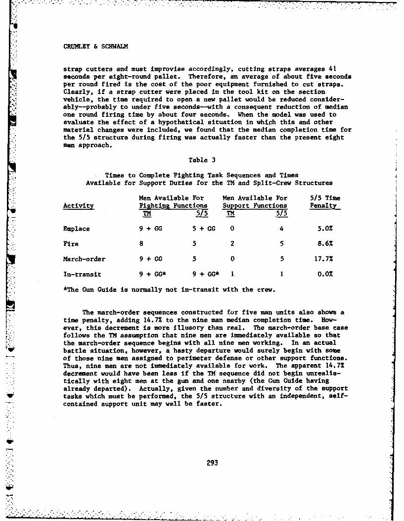
CRUMLEY & SCHWALM
strap cutters and must improvise accordingly, cutting straps averages 41seconds per eight-round pallet. Therefore, an average of about five secondsper round fired is the cost of the poor equipment furnished to cut straps.Clearly, if a strap cutter were placed in the tool kit on the sectionvehicle, the time required to open a new pallet would be reduced consider-ably--probably to under five seconds--with a consequent reduction of medianone round firing time by about four seconds. When the model was used toevaluate the effect of a hypothetical situation in which this and othermateriel changes were included, we found that the median completion time forthe 5/5 structure during firing was actually faster than the present eightman approach.
Table 3
Times to Complete Fighting Task Sequences and TimesAvailable for Support Duties for the TM and Split-Crew Structures
Men Available For Men Available For 5/5 TimeActivity Fighting Functions Support Functions Penalty
TM 5/5 TM 5/5
Emplace 9 + GG 5 + GG 0 4 5.0%
Fire 8 5 2 5 8.6%
March-order 9 + GG 5 0 5 17.7%
In-transit 9 + GG* 9 + GG* 1 1 0.O
*The Gun Guide is normally not in-transit with the crew.
The march-order sequences constructed for five man units also shows a
time penalty, adding 14.7% to the nine man median completion time. How-
ever, this decrement is more Illusory than real. The march-order base casefollows the TM assumption that nine men are immediately available so thatthe march-order sequence begins with all nine men working. In an actualbattle situation, however, a hasty departure would surely begin with someof those nine men assigned to perimeter defense or other support functions.Thus, nine men are not immediately available for work. The apparent 14.7%decrement would have been less if the TM sequence did not begin unrealis-tically with eight men at the gun and one nearby (the Gun Guide havingalready departed). Actually, given the number and diversity of the supporttasks which must be performed, the 515 structure with an independent, self-contained support unit may well be faster.
293
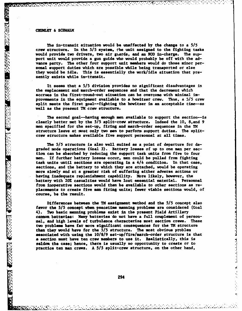
=5.
CRUNLEY &SCHWALM(
The In-transit situation would be unaffected by the change to a 5/5crew structure. In the 5/5 system, the unit assigned to the fighting taskswould provide two drivers, two air giards, and an NCO In-charge. The sup-port unit would provide a gun guide who would probably be off with the ad-vance party. The other four support unit members would do those minor per-sonal support duties which are possible while being transported or elsethey would be idle. This is essentially the work/idle situation that pre-sently exists hile in-transit.
It seems that a 5/5 division provides no significant disadvantages inthe emplacement and march-order sequences and that the decrement whichaccrues in the first-round-out situation can be overcome with minimal im-provements in the equipment available to a howitzer crew. Thus, a 5/5 crewsplit meets the first goal--fighting the howitzer in an acceptable time--aswell as the present TM crew structure.
The second goal-having enough men available to support the section--isclearly better met by the 5/5 split-crew structure. Indeed the 10, 8,and 9
men specified for the set-up, firing and march-order sequences in the TMstructure leave at most only two men to perform support duties. The split-crew structure makes available five support personnel at all times.
The 5/5 structure is also well suited as a point of departure for de-graded mode operations (Goal 3). Battery losses of up to one man per sec-tion can be absorbed by reducing the support task units from five to fourmen. If further battery losses occur, men could be pulled from fightingtask units until sections are operating in a 4/4 condition. In that case,sections, and the battery to which they are attached, would be operatingmore slowly and at a greater risk of suffering either adverse actions or-having inadequate replenishment capability. More likely, however, thebattery with 202 casualties would have lost essential materiel. Personnelfrom inoperative sections would then be available to other sections as re-placements to create five man firing units; fewer viable sections would, ofcourse, be the result.
Differences between the TN assignment method and the 5/5 concept alsofavor the 5/5 concept when peacetime manning problems are considered (Goal4). Two basic ianning problems exist in the present Field Artillerycannon batteries: Many batteries do not have a full complement of person-nel, and high levels of turbulence characterize most section crews. Thesetwo problems have far more significant consequences for the TM structurethan they would have for the 5/5 structure. The most obvious problemassociated with using the 10/8/9 set-up/fire/march-order structure is that& section must have ten crew members to use it. Realistically, this isseldom the case; hence, there is usually no opportunity to create or to'practice ten man crews. A 5/5 split-crew structure, on the other hand,
294'.. '
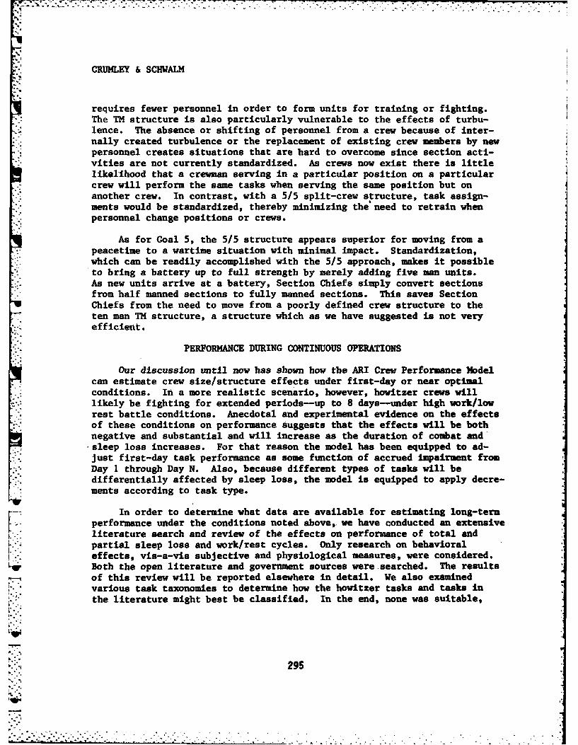
.4
CRUMLEY & SCHWALM
requires fewer personnel in order to form units for training or fighting.The TM structure is also particularly vulnerable to the effects of turbu-lence. The absence or shifting of personnel from a crew because of inter-
"* nally created turbulence or the replacement of existing crew members by newpersonnel creates situations that are hard to overcome since section acti-vities are not currently standardized. As crews now exist there is littlelikelihood that a crewman serving in a particular position on a particularcrew will perform the same tasks when serving the same position but onanother crew. In contrast, with a 5/5 split-crew structure, task assign-ments would be standardized, thereby minimizing the need to retrain whenpersonnel change positions or crews.
As for Goal 5, the 5/5 structure appears superior for moving from apeacetime to a wartime situation with minimal impact. Standardization,which can be readily accomplished with the 5/5 approach, makes it possibleto bring a battery up to full strength by merely adding five man units.As new units arrive at a battery, Section Chiefs simply convert sectionsfrom half manned sections to fully manned sections. This saves SectionChiefs from the need to move from a poorly defined crew structure to theten man TM structure, a structure which as we have suggested is not veryefficient.
PERFORMANCE DURING CONTINUOUS OPERATIONS
Our discussion until now has shown how the ARI Crew Performance Modelcan estimate crew size/structure effects under first-day or near optimalconditions. In a more realistic scenario, however, howitzer crews willlikely be fighting for extended periods-up to 8 days-under high work/lowrest battle conditions. Anecdotal and experimental evidence on the effectsof these conditions on performance suggests that the effects will be bothnegative and substantial and will increase as the duration of combat and* sleep loss increases. For that reason the model has been equipped to ad-just first-day task performance as some function of accrued impairment fromDay I through Day N. Also, because different types of tasks will bedifferentially affected by sleep loss, the model is equipped to apply decre-
S.: ments according to task type.
In order to determine what data are available for estimating long-termperformance under the conditions noted above, we have conducted an extensiveliterature search and review of the effects on performance of total andpartial sleep loss and work/rest cycles. Only research on behavioraleffects, vis-a-vis subjective and physiological measures, were considered.Both the open literature and government sources were searched. The resultsof this review will be reported elsewhere in detail. We also examinedvarious task taxonomies to determine how the howitzer tasks and tasks inthe literature might best be classified. In the end, none was suitable,
295#Inc
&i
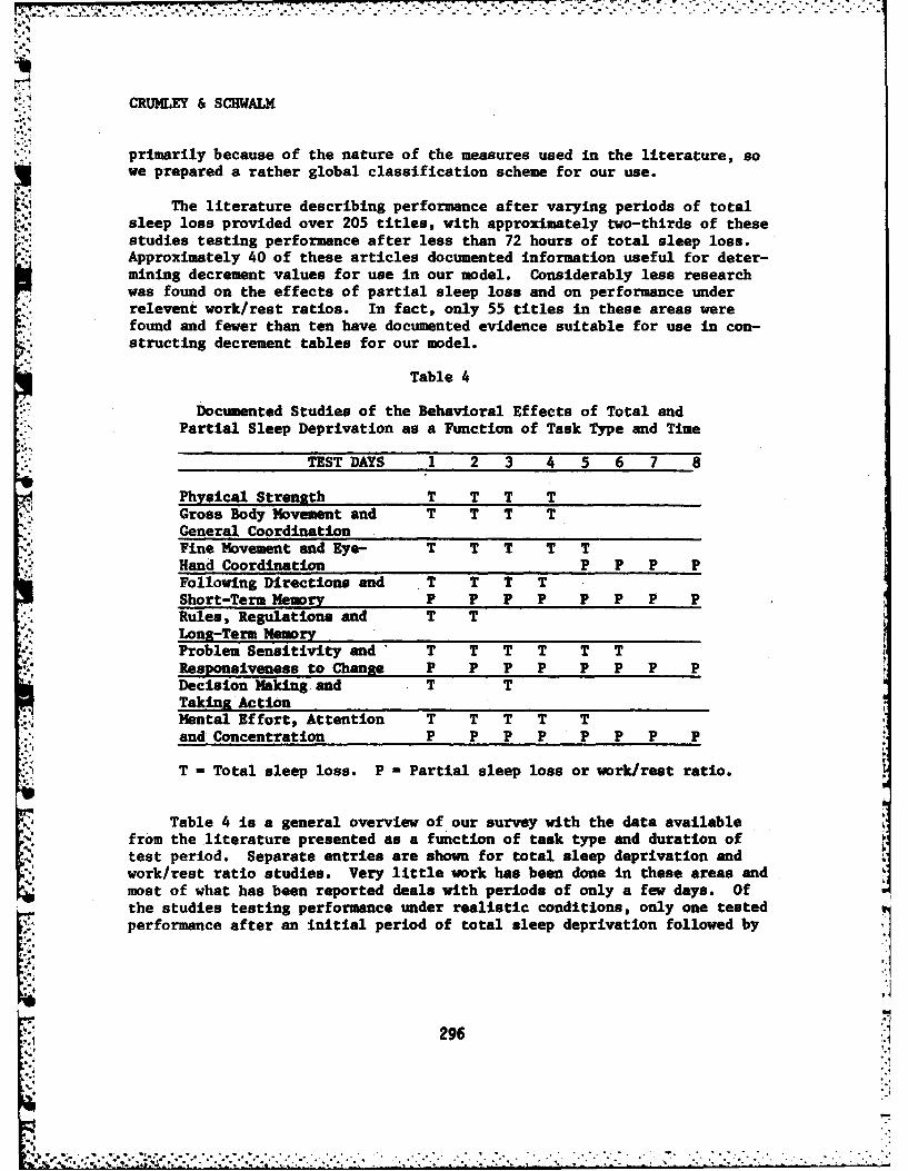
CRUMLEY & SCHWALM
primarily because of the nature of the measures used in the literature, sowe prepared a rather global classification scheme for our use.
The literature describing performance after varying periods of totalsleep loss provided over 205 titles, with approximately two-thirds of thesestudies testing performance after less than 72 hours of total sleep loss.Approximately 40 of these articles documented information useful for deter-mining decrement values for use in our model. Considerably less researchwas found on the effects of partial sleep loss and on performance underrelevent work/rest ratios. In fact, only 55 titles in these areas werefound and fewer than ten have documented evidence suitable for use in con-structing decrement tables for our model.
Table 4
Documented Studies of the Behavioral Effects of Total andPartial Sleep Deprivation as a Function of Task Type and Time
TEST DAYS 1 2 3 4 5 6 7 8
Physical Strength T T T TGross Body Movement and T T T TGeneral CoordinationFine Movement and Eye- T T T T THand Coordination P P P PFollowing Directions and T T T TShort-Term Memory P P P P P P P PRules, Regulations and T TLong-Term MemoryProblem Sensitivity and T T T T T TResponsiveness to Change P P P P P P P PDecision Making. and T TTaking Action
Al Mental Effort, Attention T T T T Tand Concentration P P P P P P P P
T = Total sleep loss. P - Partial sleep loss or work/rest ratio.
Table 4 is a general overview of our survey with the data availablefrom the literature presented as a function of task type and duration oftest period. Separate entries are shown for total sleep deprivation andwork/rest ratio studies. Very little work has been done in these areas andmost of what has been reported deals with periods of only a few days. Ofthe studies testing performance under realistic conditions, only one testedperformance after an initial period of total sleep deprivation followed by
296
. . . .7
CRUNLEY & SCHWAIM
periods when four hours of sleep per day--the maximum likely--were allowed.Some task types are notable for their lack of research documentation.Furthermore, within task types, a failure to standardize tasks and proce-dures contributes to considerable difficulty in interpreting results. In-deed, most of the studies represented in Table 4 suffer from one or moremethodological problems of varying degrees of severity. Quite common, forinstance, is failure to control for learning or circadian rhythm effects.
Thus, an extensive review of the literature on the effects of extendedperformance with reduced sleep illustrates the dearth of useful informationavailable. For this reason, only a portion of the decrement table for usewith the model can be completed based on data in the available literature,and even that portion, because of problems in the original research, is oflimited value.
CONCLUSION
The ARI Crew Performance Model can be used as an analytic tool for
evaluating the effects of crew structure on performance. Whether used withdeveloping systems or systems in the field, the model can be of value indetermining the effects of changes in crew size and the assignment of taskson the relative efficiency of varying crew structures. However, before themodel can be fully utilized, particularly when crew performance in a realis-tic battlefield scenario is being considered, a great deal of work remainsto be done to determine the effects on human performance of extended, con-tinuous performance under conditions of high work/low rest periods.
REFEPNCES
1. Schwalm, R. C., Crumley, L. H., Coke, J. S., & Sachs, S. A. A descrip-tion of the ARI Crew Performance Model (RR 1324). Fort Sill, OK:U. S. Army Research Institute for the Behavioral and Social Sciences,1981.
2. Coke, J. S., Crumley, L. H., & Schwalm, R. C. Emplacing, firing andmarch-orderina an MI09AI howitzer: Tanka anti I ion tm. (RR 1312).Fort Sill, OK: U. S. Army Research Institute for the Behavioraland Social Sciences, 1981.
3. Department of the Army. Technical manual operation and maintenancemanual (User) for howitzer, medium, self-propelled: 155mm. M109A1(2350-00-485-9622) (TM 9-2350-217-ION). Washington, DC: Head-quarters, Department of the Army, 1978.
297
, :-.;._' -.,.- .. -. ,, , .- ,,.. . ., - .. -. ..-. - - - _- - - .. . - . . - .- - , , -.. ,- .-.- . -, - , - , ,
--* UYUT O & ZE
T-. DEVZLOP T AND EVALUATION OF HDOGLOBINSOLUTION AS A BLOOD SUBSTITUTE (U)
tMI3AK DEVENUTO, Ph.D.ANGELO I. ZEGNA
LETTISNE ANIT INSTITUTE 0 RESEARCHDIVISION 01 BLOOD RESEARCH
PRESD1O 07 SAN FRANCISCO, CA 94129
The concept of using hmglobin (ib) solution as a resuscitation fluidin blood replacement therapy has been advocated for many years and has ledto extensive in vitro and in vivo investigations (1,2). These studies havebeen pursued for several reasons. One of the reasons is that blood, ascarse and valuable resource, has a limited storage life, which at presentdoes not exceed 35 days and requires specialized expertise and equipmentfor its collection, transportation, storage and pre-transfusion preparationsuch as typing and crose-matching. Furthermore, problems have occurredduring and after transfusion of blood. These problems include hemolytictransfusion reactions, allergic reactions, circulatory overload, embolism,citrate toxicity, coasulation disturbance and the transmission of disease(3-4). Therefore, a strong Incentive exists for finding a suitable resus-citatig solution ubch would alleviate or minimize such problems.
Aother reaso for the development of an effective blood substitute isthe ability to admaister the resuscitating solution to the patientsdirectly at the place where the injury causin logo of blood volume hasoccurred, without requiremant for transportation of patients to treatmentcenters or medical facilities. Thms, Imediate medical assistance byrestoration of blood volume and oxygen carrying capacity will greatlyincrease the chances for survival. Futherore, a stable resuscitatingsolution can be stockpiled and, therefore, can minimise the logistic pro-blem of supply,, storage and transportation which occur when large quanti-ties of fluid replacement are necessary in ma casualties.
Significant advantages can be gainl by the development of a resusci-tating solution capable of transporting oxygen, maintaining oncoticpressure, and being readily available when massive transfusions are re-quired. Stringent requirements mast be net for a resuscitating solutionIn order to be effective. As a blood substitute, this solution not onlymst be capable of restoring vital functions, but mast not elicit perma-nent adverse effects when administered to patients.
: I- '299
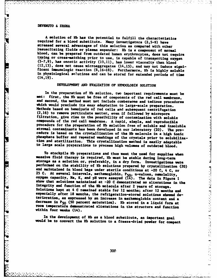
DEVEHUTO & ZEGNA
A solution of Hb has the potential to fulfill the characteristicsrequired for a blood substitute. Many investigators (2,5-9) havestressed several advantages of this solution as compared with otherresuscitating fluids or plasma expander: Rb is a component of normalblood, can be prepared from outdated human erythrocytes, does not requiretyping or cross-matching prior to use, is capable of transporting oxygen(5-7,9), has oncotic activity (10,11), has lover viscosity than blood(12,13), does not cause microaggregates (14,15), and may not induce signi-ficant ismunologic reaction (8,16-18). Furthermore, Hb is highly solublein physiological solutions and can be stored for extended periods of time(14,19).
DEVELOPMENT AND EVALUATION OF HEMOGLOBIN SOLUTION
In the preparation of Hb solution, two important requirements must bemot: first, the Rb must be free of components of the red cell membrane,and second, the method must not include cumbersome and tedious procedureswhich would preclude its easy adaptation to large-scale preparation.Methods based on hemolysis of red cells and subsequent centrifugation(2,16) to remove particulate matter, even if followed by microporefiltration, give rise to the possibility of contamination with soluble.compounds of the red cell membrane. A rapid, simple, and reproducibleprocedure for the preparation of Hb solution free of soluble and insolublestromal contaminants has been developed in our laboratory (20). The pro-cedure is based on the crystallization of the Hb molecule in a high ionicphosphate buffer and repeated washings of the crystals prior to solubiliza-tion and sterilization. This crystallization method is easily adaptableto large scale preparations to process high volumes of outdated blood.
To stockpile Hb preparations and thus meet the need for supplies whenmassive fluid therapy is required, Hb must be stable during long-termstorage as a solution or, preferably, in a dry form. Investigations wereperformed on the stability of Rb solutions prepared by crystallization (20)and maintained in blood bags under sterile conditions at -20 C, 4 C, or25 C. At several intervals, methemoglobin, Pg n-values, oemolality,oxygen capacity, Na, K, and pH were assayed (R;. The data In Figure 1show that solutions maintained at -20 C demonstrated no alterations In theintegrity and function of the 1Kb molecule after 2 years of storage.Solutions kept at 4 C remained stable for 12 months; after 12 months andespecially after 18 months, the refrigeration-stored solutions showed de-terioration, as expressed by an increase in methemoglobin content and adecrease in P5 (50 percent saturation). Rb stored in a liquid form atroom temperature demonstrated alterations in the structure and functionwithin four weeks (14).
In the development of Hb as a blood substitute, an important goalwould be to convert the Hb solution to a freeze-dried powder for compact
300
5 . - - . -* - - .. ...
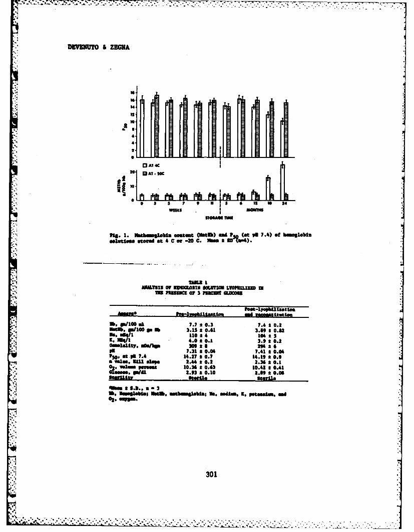
DIVENUTO & ZEGNA
.4 Ia1412
10
0 Nl1% fhA t I2 I 2 0 2
0A14C OI [Lh.I.iebamglobi cstent (tb) and P (at ON 7.4) of bomgloblu
slutiona stored at 4 C or -20 C. lbm 2 U'?uum4)
MALTIKS f UWWO31 UKITIULOULZD
IN PIM=C OF 3 PIIKUT 61006
*. P10 al 7.7 * 0.3 7.4 2 0.2NIM. w/100 go-b 3.13 & 0.41 3.89 * 0.62me, owl 110 24 104*15K, "I1 4.0 *0.1 3.9*20.2
a Ity. of/11 309 t6 294 26
98 a l . 7.31*a0.06 7:41*20.04
aVloansoe2.44 2 0.2 2.26 * 0.1402- wiM Pevoeme 10.36 * 0.63 10.412 *0.41
GLOOM.s P/dl 2.932*0.10 2.89*20.0063e9ulty Itetilh Ste
4 Me 80gSUia; *140, mstbumgSUa; See aSWIim 1, potassium. md
301
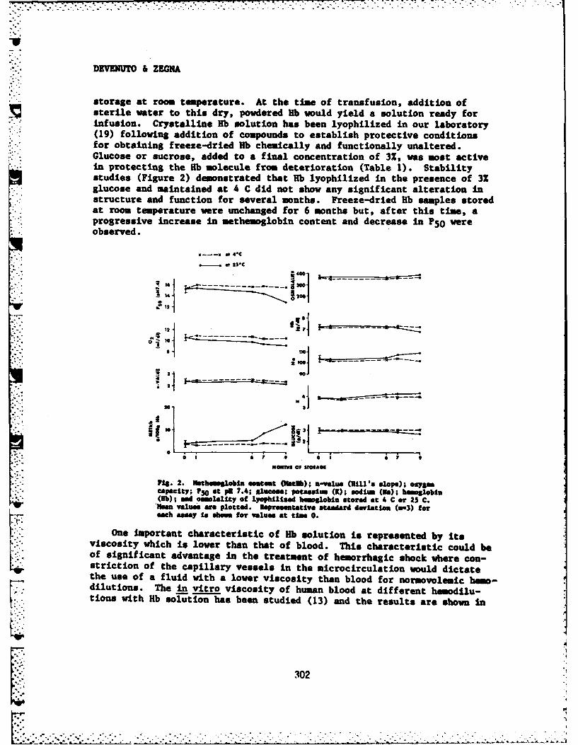
DEVINUTO & ZEGNA
storage at room temperature. At the time of transfusion, addition ofsterile water to this dry, powdered Rb would yield a solution ready forinfusion. Crystalline Rb solution has been lyophilized in our laboratory(19) following addition of compounds to establish protective conditions
- for obtaining freeze-dried Rb chemically and functionally unaltered.Glucose or sucrose, added to a final concentration of 3%, was most activein protecting the Rb molecule from deterioration (Table 1). Stabilitystudies (Figure 2) demonstrated that Rb lyophilized in the presence of 32glucose and maintained at 4 C did not show any significant alteration instructure and function for several months. Freeze-dried Hb samples storedat room temperature were unchanged for 6 months but, after this time, aprogressive increase n methemoglobin content and decrease in P5 0 wereobserved.
d 44C
so.
----------- "
SI~O S ? 0 I01" - MONVM5 0 S?01*OI
yiS. 2. Sethmbolbin content (Ntb); n-value (8111's slope); oxygzecapeity; PSO at pi 7.4; Aluaeose potasaim (K); sodium (Na); hesalobin(Nb); ead oomei0lity of 1ophllsed bhmoslobis stored at 4 C or 25 C.MVan values we plotted. Repre etative standard deviation (nu3) for
each assay Is .h.. for values at time 0.
One important characteristic of Hb solution is represented by itsviscosity which is lower than that of blood. This characteristic could beof significant advantage in the treatment of hemorrhagic shock where con-striction of the capillary vessels in the microcirculation would dictatethe use of a fluid with a lower viscosity than blood for normovolemic hemo-dilutions. The in vitro viscosity of human blood at different hemodilu-tions with Hb solution has been studied (13) and the results are shown in72
302
.. . . .
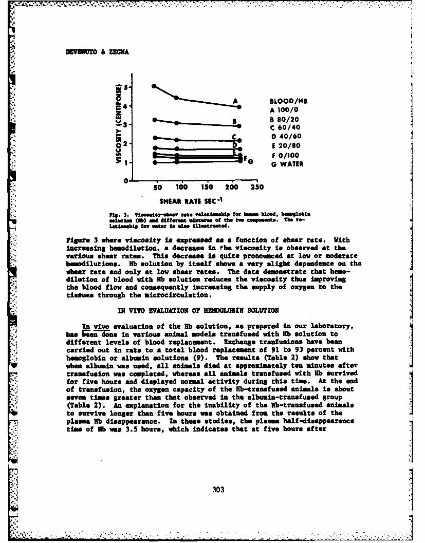
o - & ZEGMA
A BLOOD/HBZ4 A 100/0rM
- B 80/20" - C 60/40
- C- D 40/6002- D -E 20/0
S1F F 0/100G WATER
0*50 100 10 2o 250
SHEAR RATE SEC- 1
S18. 3. vWaeoolthbeer rate relatoma1lp for bhmen blood, bhmo8loblnsolution (9b) oid diffetart adwoure of the tw c.Woin-ta. The re-,aSt lolhp for water Ieloo llautrmted.
Figure 3 where viscosity is expressed as a function of shear rate. WithIncreasing hemodilution, a decrease in the viscosity is observed at the
* :various shear rates. This decrease is quite pronounced at low or moderatehooodilutions. fb solution by itself shows a very slight dependence on theshear rate and only at low shear rates The date demonstrate that hems-dilution of blood with fb solution reduces the viscosity thus Improvingthe blood flow and consequently increasing the supply of oxygen to thetissues through the microcirculation.
IN VIVO EVALUATION OF HEMOGLOBIN SOLUTION
In vivo evaluation of the fib solution, as prepared in our laboratory,has been done in various animal models transfused with fib solution todifferent levels of blood replacement. Exchange tranfusions have beencarried out in rats to a total blood replacement of 91 to 93 percent withhemoglobin or albumin solutions (9). The results (Table 2) show thatwhen albumin was used, all animals died at approximately ten minutes aftertransfusion was completed, whereas all animals transfused with fib survivedfor five hours and displayed normal activity during this time. At the endof transfusion, the oxygen capacity of the fib-transfused animals is aboutseven times greater than that observed in the albumin-transfused group
-,' (Table 2). An explanation for the Inability of the Hb-transfused animalsto survive longer than five hours was obtained from the results of theplasma ib disappearance. In these studies, the plasma half-disappearancetime of Hb was 3.5 hours, which indicates that at five hours after
; . 303
<7 C<.W- .:
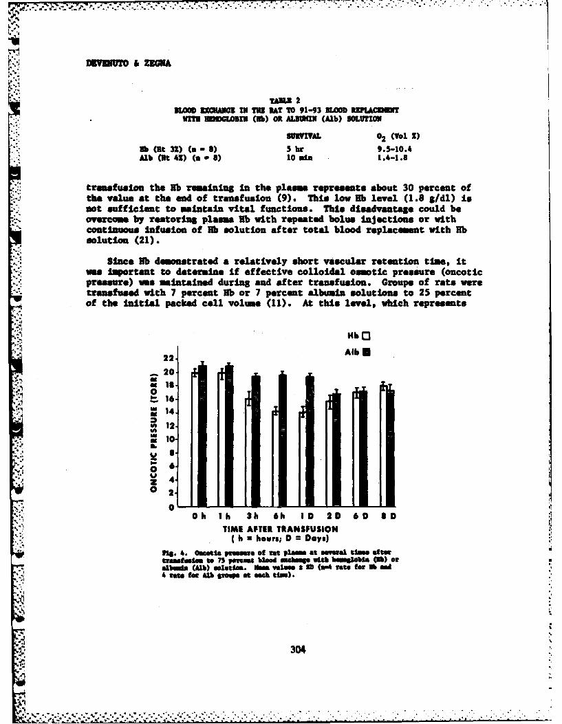
TANA! 2BLOOD UCHAUGZK I T RAT T0 91-93 BLOOD UBILACUUU
luTI! IIbDCLODXU (11b) OR ALBUMEI (Alb) SOLUTION
SURVIAL. 02 (Vol X)
Bb (Bt 32) (a * 8) 5 hr 9.5-10.4Alb (Ht 41) (a w 6) 10 a1.-.
transfusion the Rb remaining In the plasma represents about 30 percent ofthe value at the end of transfusion (9). This low Rb level (1.8 g/dl) Isnot sufficient to maintain vital functions.* This disadvantage could beovercome by restoring plaws Rb with repeated bolus Injections or withcontinuous Infusion Of Rb solution after total blood replacement with Rbsolution (21).
* Since Rb demonstrated a relatively short vascular retention time, itmes Important to determine if effective colloidal osmotic pressure (oncoticpressure) 10s Maintained during and after transfusion. Groups of rats weretransfused with 7 percent Rb or 7 percent albumin solutions to 25 percentof the Initial packed cell volume (11). At this level, which represents
UbO3
22. AlbE
~20.IZa is
0M 16-
12..10-
0 2.0
Oh Ii, 3h. 60% 1D 2D 6 D 4 DTIME AFTR TRWANSUION
(h *hours; D = Days)no. 4. ousetia Prei of rat Plais at mweral tsles after
tramfusltoa 75 pereeme bUsed ombes th bamaeis C9b) orelbsoia (Clb) esleim. YAM. ValIS a 3 (wmA rate for Nb sad4 rate for Alb goew at each ta.).
304
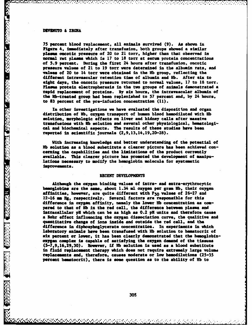
*77
DUYUWTO & ZEGNA
75 percent blood replacement, all animals survived (9). As shown inFigure 4, Imediately after transfusion, both groups shoved a similarplasma oucotic pressure of 20 to 21 tort, higher than that observed innormal rat plasma which is 17 to 18 torr at serum protein concentrationsof 5.9 percent. During the first 24 hours after transfusion, oncoticpressure values of 21 to 19 torr were determined in the albumin rats, andvalues of 20 to 14 torr were obtained In the lb group, reflecting thedifferent intravascular retention tine of albumin and Hb. After six toeight days, the oncotic pressure returned to normal values, 17 to 18 torr.Flama protein electropheresis in the two groups of animals demonstrated arapid replacement of proteins. By six hours, the intravascular albumin ofthe lb-treated group had been replenished to 57 percent and, by 24 hours,to 83 percent of the pre-infusion concentration (11).
In other investigations we have evaluated the disposition and organdistribution of Hb, oxygen transport of human blood hemodiluted with lbsolution, orphologic effects on liver and kidney cells after massivetransfusions with lb solution and several other physiological, hematologi-cal. and biochemical aspects. The results of these studies have beenreported in stientific journals (2,9,13,14,19,20-28).
N With Increasing knowledge and better understanding of the potential oflb solution as a blood substitute a clearer picture has been achieved con-cerning the capabilities and the limitations of the product currentlyavailable. This clearer picture has promoted the development of manipu-lations necessary to modify the hemoglobin molecule for systematicImprovements.
RECENT DEVELOPNKNT
Although the oxygen bindi g values of intra- and extra-erythrocytichemoglobins are the same, about 1.34 mul oxygen per graS Rb, their oxygenaffinities, however, are quite different with PSO values of 26-27 and12-16 a Hg, respectively. Several factors are responsible for thisdifference in oxygen affinity, namely the lower lb concentration as com-pared to that of lb in the red cell, the difference between plasma andintracellular pH which can be as high as 0.2 pH units and therefore causea Bohr effect influencing the oxygen dissociation curve, the qualitive andquantitative change of Ions inside and outside the red cell, and thedifference in diphosphoglycerate concentration. In experiments in whichlaboratory animals have been transfused with lb solution to hematocrit ofsix percent or lower, it has been clearly demonstrated that the hemoglobin-oxygen complex Is capable of satisfying the oxygen demand of the tissues(5-7,9,16,29,30). However, If lb solution is used as a blood substitutein fluid replacement therapy which does not require extremely large volumereplacements and, therefore, causes moderate or low hemodIutions (25-35percent hematocrit), there Is some question as to the ability of lb to
305
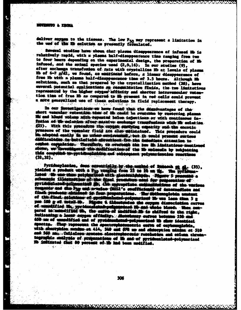
delivr eappe to the tiesue h on Up mpsy, rorset a ]llataetin1
5*01d vsfte hanew hmht pleaK dippesra.e of "ftnd a6 ioreltivlyrapiw, Uteh at pass" heltfdiesppraeo. tim rsmug t twofl
to tfew boai dpaduss -n the .upnbata-" di~so the ppaUs of NbSalvs, and fke aam*4 petee mwt (2,941*) * T our stude. (9,att mcmw emtnae.* .1 S rate f ettaluspe lb- at law!. of pleinab of 6-Q1 aft.& we hun, -~~tW hoem., a tUie Separus. .1
11b .2t 1h baa2 1e.sitions, musk asv that porepareS hr th cryetsll1taaelwu td (20)v have
usO seo of, free ]Rb a. capMeS to tb peamt I^ rd ceLl aomid, unmst,ato re g.evelad uee of theeb sobuetam ft fluid "Iplcese therapy.
IStnhMr. thfttto -mhe f ats a that .u Ohf pr *Seos
Lt St US ak ur(51)
ct
fl5Yfl41oomf ad IS1- 001SWpia Ww Sam, 5
sw~
-~~~~~~~~~ .r r r. ;- - #r P g 4'W 'Pv
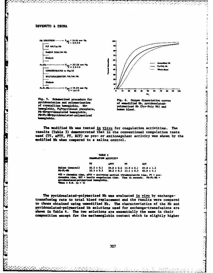
DKVENUTO &ZEGA
Mb SOLUTION - P50 = 14.16 Hm Wga = 2.4-2.6-- - - - - - - - - -
KIP 4M/M bW
NQH4 2OM/AM Hb
Ph.Hb P50 23.26 mmn He so/ -- UWd In.a 2.3-2.5 P 6,M
CONCENTSATED to 149/dI 4 160Sn
*LUTARALDIHTDE 7M/1M Mb
Dialysis
fth-ib-NhO1-2 mH
7U.* 5. Scebmntixod procedure for 719. G. Ozgm d1*OociLattot CurvesWIdoaalatlon ad polymerizatlon of uao dif led Rb, pyridozalated-
* .Of Crystallbne bmgolobln. Ilbm poymerised Rb (Pyr-?oly Kb) andbansalbln, flPmpyrldozal phosphate, bmann blood.Pi-MmMyrdozalated hesiolob~n,MR-U3MIpyr~dozalated-polywerlzedbamsgbla.
The modified lb was tested In vitro for coagulation activities. Theresults (Table 3) demonstrated that in the conventional coagulation teatsused (TT, alif, PT, KCT) no pro- or anticoagulant activity was shown by theJmodified fib when compared to a saline control.
TAMA 3GDA!ULA11 ACYTTM*
Tr AIPT IPT KCTSall"s (smml) 22.5 * 0.1 29.8 * 0.6 12.9 t 0.1 83.8 a 1.2
13na22.3 * 0.3 30.2 * 0.3 13.1 a 0.3 65.8 t 4.1ft! - Sh~tas AM. ali uactiVated partial thromboplastla tine, nT - pro-thnn~a tie, WT - haolin ompglation tie. Time in secend.. PK--Bb
Alea * S.D. (a - 3)
The pyridoxalated-polymerized lb was evaluated in vivo by exchange-transfusing rats to total blood replacement and the results were comparedto those obtained using unumodified lb. The characteristics of the Rb andpyridozalated-polymerized 1hb solutions used for exchange-transfusions areshown In Table 4. The two solutions are essentially the same in their
coposition except for the methemoglobin content which is slightly higher
f1 307
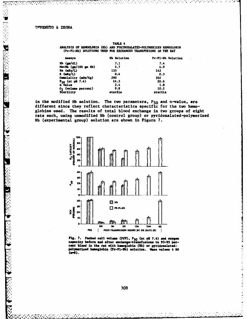
. t ...... .
1.FVENUTO & ZEGNA
TABLE 4ANALYSIS OF HEBLOBIN (Hb) AND PYRIDOXALATED-POLYHERIZED HENDGLOBIN
(Pr-PI-Ib) SOLUTIONS USED FOR EXCHANGED TRANSFUSIONS IN THE RAT
Assays Rb Solution Pr-Pl-Hb Solution
Nb (So/dl) 7.1 7.4Natib (gm/100 go Hb) 2.7 4.9Ne (*Zq/L) 135 142K (uq/L) 0.4 0.3Omoolality (moW/KS) 290 302P5 (at pH 7.4) 14.3 20.6n value 2.4 1.802 (volume percent) 9.8 10.2Sterility sterile sterile
in the modified Hb solution. The two parameters, P50 and n-value, aredifferent since they reflect characteristics specific for the two hemo-globins used. The results of total blood exchange in two groups of eightrats each, using unmodified lib (control group) or pyridoxalated-polymerizedHb (experimental group) solution are shown in Figure 7.
100-
40-
20"
:oSo o-
4
0
a. 20
40 b 40
0 3 0
220-
,. ..- i p . .
20-
ON 3M SN 12H 24H s
I POSt.YTANSFUSION HOURS ("I ON DAYS 10)
Fig. 7. Packed cell voltme (PCV), P5 (at ptl 7.4) sad oxygencaaity before enad after emcbange-tranefustiona to 93-95 per-cet blood In the rat with hemoglobln (Nb) or pyridoxalated-polymerised hioglobin (P-PI-b) solution. an values ± SD.'. "( IN O ) .
.'." 308"
' ... . . . . . . .. . . . . . . . . . . . . . . . . . . . . . . .
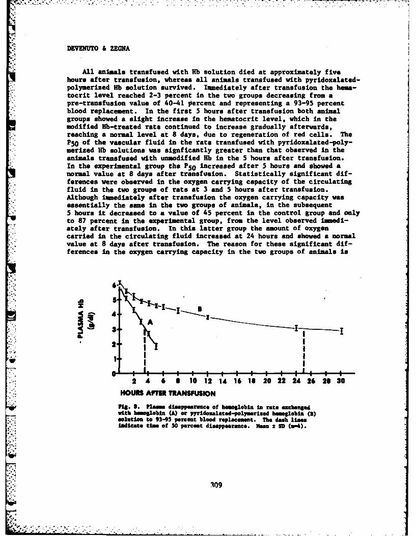
DEVENUTO & ZEGNA
All anisals transfused with Hb solution died at approximately fivehours after transfusion, whereas all animals transfused with pyridoxalated-polymerized Hb solution survived. Immediately after transfusion the hems-tocrit level reached 2-3 percent in the two groups decreasing from apre-transfusion value of 40-41 percent and representing a 93-95 percentblood replacement. In the first 5 hours after transfusion both animalgroups showed a slight increase in the hematocrit level, which in themodified Hb-treated rats continued to increase gradually afterwards,
* reaching a normal level at 8 days, due to regeneration of red cells. TheP50 of the vascular fluid in the rats transfused with pyridoxalated-poly-merized Kb solutions was signficantly greater than that observed in the
* . animals transfused with unmodified Hb in the 5 hours after transfusion.In the experimental group the P50 increased after 5 hours and showed anormal value at 8 days after transfusion. Statistically significant dif-ferences were observed in the oxygen carrying capacity of the circulatingfluid in the two groups of rats at 3 and 5 hours after transfusion.Although immediately after transfusion the oxygen carrying capacity wasessentially the same in the two groups of animals, in the subsequent5 hours it decreased to a value of 45 percent in the control group and onlyto 87 percent in the experimental group, from the level observed Immedi-ately after transfusion. In this latter group the amount of oxygencarried n the circulating fluid increased at 24 hours and showed a normalvalue at 8 days after transfusion. The reason for these significant dif-ferences in the oxygen carrying capacity in the two groups of animals is
a 5
z6
A
4-I
2 4 6 1 10 12 14 16 18 2 2 24 26 2 0
HOURS AfTIR TRANSFUSION
1g. S. Plum diappearace of heosslobin in rate ezchangedw!th bmsglobla (A) or pyrdoxalatd-polmmrized hemoglobin (3)oliuton to 93-95 percent blood replacement. The dash linee
Indicate tme of 50 percent disappearance. NMan 2 SD (m-).
. : - -, , - . - , , . - . • , . . - , .
DEVENUTO &ZEGNA
found in the rate of disappearance of plasma Hb which is shown In Figure 8for two groups of four rats each, control and experimental group. Thedata in Figure 8 demonstrate that the plasma disappearance of Hb wasfaster in the Hb-treated than in the modified b-transfused animals. Theplasma half-disappearance time, that is the time necessary for the plasmaHb concentration to reach one half the value observed at the end ofexchange-transfusion was 3.5 hours for the control groups and 25 hours forthe experimental group.
It appears, therefore, that the two limitations of higher oxygenaffinity and lower intravascular retention of Hb can be overcome by themodification of the Hb molecule. The administration of a solution ofpyridoxalated-polymerized Hb appears to be beneficial in total blood re-placement since it promotes survival of the animals. We have investigatedmorphological effects on various organs, and preliminary studies have de-monstrated that kidney and liver cell structures remain normal; however,other potential effects which may occur after massive transfusion with
-- pyridoxalated-polymerized Rb solution must be studied in order to evaluatethe significant potential value of this solution as a blood substitute.
CONCLUSIONS
The development and evaluation of an effective Rb solution as a bloodsubstitute are important not only for the care of casualties resultingfrom mass disasters, but also for eventual use in other special clinicalsituations. Substantial improvements have been made by several recentresearch efforts in the general purity and quality of experimental Rb so-lutions. Such improvments have enabled investigators to study thepotential applications of Hb solutions in far less ambiguous manner thanwas previously possible. These studies have produced a reasonably clearpicture of the limitations of the current product and an insight forapproaches In a systematic Improvement.
The Hb solution as presently formulated, although has the limitationof short vascular retention time, potentially could be useful in severalapplications such as transfusions in patients vw cannot receive Inmedi-ate medical assistance, but could receive blood after a few hours, ortransfusions In patients who cannot receive medical care for prolongedperiods of time, provided that the Rb and blood volume losses are restoredby periodic or continuous infusion of Rb solution. Furthermore, the pre-sent product could be useful in open heart surgery, in organ perfusion andin situations of uncontrolled bleeding.
It is hoped that research studies involved with modification of Rb,aimed at maintaining the tetrameric molecule in vivo, may provide a stableHb compound having longer intrascular life as well as lower oxygen
310
2. ..
o -~ ~
-,4
DIVNUTO & ZEMNA
affinity and that the remaiLing issues could be clarified so that thisblood substitute can be beneficial to man.
REFERENCES
1. Amberson VR: Blood substitutes. Biol Rev 12:48-86, 1937.2. DeVenuto F, Friedman HI, Neville JR, Peck CC: Appraisal of hemoglobin
solution as a blood substitute. Surg Gynecol Obstet 149:417-436,1979.
3. Gruber VF: Blood replacement. Springer-VERLAC, Berlin, 1969.4. Huestis DW, Bove JR, Busch S: Practical blood transfusion. 2nd ed.,
Little, Brown, Boston, 1976.5. Bonhard K: Acute oxygen supply by infusion of hemoglobin solutions.
Fed Proc 34:1466-1467, 1975.6. Kaplan HR, Murthy VS: Hemoglobin solution: a potential oxygen trans-
porting plasma volume expander. Fed Proc 34:1461-1465, 1975.7. Moss, GS, Der Woskin R, Rosen AL: Transport of oxygen and carbon
dioxide by hemoglobin-saline solution in the red cell-free primate.Surg Gynecol Obstet 142:357-362, 1976.
8. Peskin CW, O'Brien K, Rabiner SF: Stroma-free hemoglobin solution:The "ideal" blood substitute? Surgery 66:185-191, 1969.
9. DeVenuto F, Moores WY, Zegna AI, Zuck TF: Total and partial bloodexchange in the rat with hemoglobin prepared by crystallization.Transfusion 17:555-562, 1977.
10. Amberson Wr, Flexner J, Steggerada FR, Mulder AC, Tendler MJ,Pancratz DS, Laug EP: On use of Ringer-Locke solutions containinghemoglobin as a substitute for normal blood In mammals. J CellCoop Physiol 5:359-382, 1934.
11. DeVenuto F, Zegna Al: Plasma oncotic pressure during and after bloodexchange with crystalline hemoglobin solution. Surg Gynecol Obstet147:379-384, 1978.
12. Usami S, Chien S, Gregersen HI: Hemoglobin solution as a plasmaexpander: Effects on blood viscosity. Proc Soc Exp Biol Med136:1232-1235, 1971.
13. DeVenuto F, Busse KR, Zegna Al: Viscosity of human blood hemodilutedwith crystalline hemoglobin solution. Transfusion 21:752-756,1981.
14. DeVenuto F: Stability of crystalline hemoglobin solution duringextended storage. J Lab Clin Med 92:946-952, 1978.
15. Hamilton PB, Farr LE, Hiller A, Van Slyke DD: Preparation of hemo-globin solutions for intravenous infusion. J Exp Med 86:455-463,1947.
4 16. Rabiner SF, Helbert JR, Lopas H, Friedman LH: Evaluation of stroma-free hemoglobin solution for use as a plasma expander. J Exp Med126:1127-1142, 1967.
311
..... ............... ... ... ...................................
DBYIMflO & ZEQIA
17. Cockin A, Des Gupta TK, Der Voskin R, Moss GS: Zurnogenic proper-ties of stroma versus stroma-free hemoglobin solutions. Surg Forum23:19-21, 1972.
i8. Sasazuki T: Studies on haptoglobin. I. Immunochemical properties ofhaptoglobin and antihemoglobin antibody. Proc Jap Acad 46:820,1970.
19. DeVenuto F, Zegna Al, Busse KR: Lyophilization of crystalline hemo-slobin solution and exchange transfusions with lyophilized,reconstituted hemoglobin. Surg Gynecol Obstet 148:69-75, 1979.
20. DeVenuto F, Zuck TV, Zegna Al, Moores WT. Characteristics of stroma-free hemoglobin prepared by crystallization. J Lab Clin Med89:509-516, 1977.
21. DeVenuto F, Friedman HI, Mellick PN: Massive transfusions withcrystalline hemoglobin solutions and subsequent replacement ofhemoglobin and blood volume. Surg Gynecol Obstet 151:361-365,1980.
22. DeVenuto F, Busse KR, Zegna AI: Oxygen transport by human bloodhemodiluted with crystalline hemoglobin solution. Surg GynecolObstet 153:332-336, 1981.
23. Zuck TF, DeVenuto F, Meville JR, Friedman HI: Oncotic and oxygentransport effects of hemoglobin solutions. Prog Clin Biol Res19:111-147, 1978.
24. Friedman HI, DeVenuto F, Zuck TF, Mellick P, Lollini L: Histologicand ultrastructural effects of stroma-free hemoglobin solution Inrat liver, kidney, and brain. Surg Forum 28:3-5, 1977.
25. Friedman RI, DeVeauto F, Lollini L, Wellick P, Zuck TI: Y&Tphologicaleffects following massive exchange transfusions with a strom-freehemoglobin solutions. I. Liver. Lab Invest 39:167-177, 1978.
26. Friedman HI, DeVenuto F, Lollini L, Mellick F, Zuck TI: Morphological Ieffects following massive exchange transfusions with a stroma-free
hemoglobin solution. 11. Kidney. Lab Invest 40: 655-667, 1979.27. Moores V1, DeVenuto F, Heydorn VS, Weiskopf RB, Baysinger. M,
Hannon JP: Improved porcine myocardial performance during severeanemia using a strosa-free hemoglobin solution. Fed Proc 39:2331,1980.
28. Moores 11!, DeVenuto F, Reydorn 191, Weiskopf RB, Baysinger BS,Greenburg AF, Utley JR: Extending the limits of hemodilution oncardiopulmonary bypass using stroma-free hemoglobin solution.J Thorac Cardiovasc Surg'81:155-162, 1981.
29. Uses JE, Hauser CJ, Shippy C, State D, Shoemaker UC: Comparison ofcardiorespiratory effects of crystalline hemoglobin, whole blood,albumin and inger's lactate In the resuscitation of hemorrhagicshock In dogs. Surgery 83:639-647, 1978.
30. Mener K, Jeach F, Schaff J, Schoenberg N, Peileticker K, Bonhard K:Oxygen supply by strome-free hemoglobin. Prog Clin Biol Res19:175-190, 1978.
312
DRVUITO & ZIZM
31.* DeVenuto U', Zegna Al: Transfusions with pyridoxalated-polymerizedhemolobin solution. Transfusion 21:599, 1981.
32. DaVesuto 1: Hemoglobin solutions as oxygen-delivering resuscitationfluids. Crit Care Ned (in press).
33. laesech 35., Benesch R, Ranthal RD, Maeda N: Affinity labeling of the* polyphosphate binding site of hemoglobin. Biochemistry
!77,
1:738 17A- "
-. "4
• ' * e0uor enaA:Tssutn ihpy~oaae-oye~e
hemoslbiu 8outlon.Transfsion313 59 91
...... ..... F imslbnsltin soxgndlve~grsuctto

*. DEVENUTO & ZEGNA
FIELD PRODUCTION OF PURIFIED STERILE WATER FROMAVAILABLE WATER SOURCES BY USING A PORTABLE APPARATUS (U)
-*FRANK DEVENUTO, PH.D.ANGELO ZEGNA
LETTEHMAZ( ARMY INSTITUTE OF RESEARCHPRESIDIO OF SAN FRANCISCO, CA 94129
The development of portable equipment for the production of pure waterfrom fresh pond, sea water, or other sources is important for militaryrequirements in field situations. Also, it is necessary for many civilianactivities whenever pure water is not available. The criteria for purityare influenced by the intended use of the water. Lake water which could beconsidered pure for swimming may not be suitable for drinking, and munici-pal water found pure for drinking is not considered pure for pharmaceuticalpreparations or for clinical use. The American Chemical Society, theAmerican Society for Testing Materials, and the College of American Path-ologists have specified various parameters for the purity of water.However, each of these agencies has proposed different standards (1),which apply for different purposes, and therefore, do not represent a uni-form guide.
According to the criteria of the United States Pharmacopeia (USP) (2),sterile water for injection is a clear, colorless, odorless liquid; it issterile without addition of antimicrobial agent or other substances, ispyrogen-free, and has a total solids content of 2 to 4 ug percent. In theusual urban environment, sterile water for injection is readily available;howsver, in field situations or in areas remote from supply sources, theprocurement of purified water could present logistic difficulties. Theproblems associated with transportation, storage, and supply of largequantities of pure sterile water can be overcome by its production in situby using any. available source of water which is purified by a simple inex-pensive process. Purified, injectable water may be needed in militaryfield situations as a diluent for pharmaceutical formulations, for pre-paration of sterile saline solutions, for reconstitution of lyophized hemo-globin for fluid therapy (3-5), for solubilization of preservatives to beadded to human blood for prolongation of its shelf life (6), for prepara-tion of solutions for the rejuvenation of outdated red blood cells (7) orfor other purposes.
315
X 0v < ,,-,.. ,. - - . .. -.. . . .. - . . - . - . . . . . . . . . . .
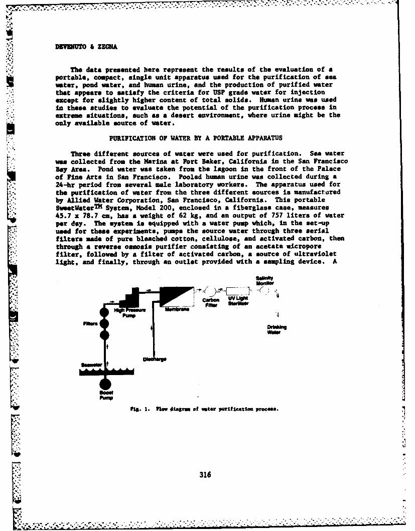
f.* . ... ... ... *.... *. .**- -
DEVEIT ZGNA
The data presented here represent the results of the evaluation of aportable, compact, single unit apparatus used for the purification of seawater, pond water, and human urine, and the production of purified waterthat appears to satisfy the criteria for USP grade water for injection
S.. except for slightly higher content of total solids. Human urine was used*: in these studies to evaluate the potential of the purification process in
extreme situations, such as a desert environment, where urine might be theonly available source of water.
PURIFICATION OF WATER BY A PORTABLE APPARATUS
Three different sources of water were used for purification. Sea waterwe collected from the Marina at Fort Baker, California in the San FranciscoBay Area. Pond water was taken from the lagoon n the front of the Palaceof Fine Arts in San Francisco. Pooled human urine was collected during a
' . 24-hr period frm several male laboratory workers. The apparatus used for
the purification of water from the three different sources is manufacturedby Allied Water Corporation, San Francisco, California. This portableSweetWater T System, Model 200, enclosed in a fiberglass case, measures45.7 x 78.7 cm, has a weight of 62 kg, and an output of 757 liters of waterper day. The system is equipped with a water pump which, in the set-upused for these experiments, pumps the source water through three serialfilters made of pure bleached cotton, cellulose, and activated carbon, thenthrough a reverse osmosis purifier consisting of an acetate microporefilter, followed by a filter of activated carbon, a source of ultravioletlight, and finally, through an outlet provided with a sampling device. A
8 4
pump-
3161
monow
316
.... .. ,...... .....-...--....-...... ....-.....-.-.. ,....., ;,,. -..! L ,7 %i . ° *%. , .- - ' * ., . -" - . * . . .- ..' . m~ w N .. - d -- .. - * * *.
' * ** *
ft ~ ~ ~ ~ ~ ~ ~ ~ o uA.i1.V . .A w..

SIKVYUTO & ZEGNA
flow diagram of the water purification process is shown in Figure 1. Inm ezperiments, a millipore Tvin-90 sterile 0.22 U filter was connected
to the outlet system prior to collection of purified water to removebcterial contamination.
The acetate micropore filter incorporated in the reverse osmosis puri-fier lasts for two years or longer if properly maintained.* It Is continu-ously rinsed by water pumped into the apparatus, thus preventing theaccumulation of particulate matter on the filter. The three serial filtersplaced before the reverse osmosis purifier and the activated carbon filterwhich follows remain effective for a period of t1a dependent on the In-purities present in the water source used. Purification of sea water in acontinuous operation requires replacement or regeneration after one weekfor the first-in-line filter and after two weeks for the other filters inorder to obtain purified water of consistent high quality. The apparatusis portable, and can be used anywhere water is needed as long as a water
* ~ supply of some source is available. It can be modified to use differentpower sources such as a combustion engine or even manpower.
RESULTS
The ion content of the water samples from sea water, fresh pond water.and human urine before and after purification are shown in Table I. The
TABLE ISION COUTT BEORE AND ATER WATER PURIFICATION
USP SEA P01M URINE
Before After Before After Before After
No (us/dl) t 0.0 1,023.05 18.39 19.54 1.15 188.52 2.30
9 (us/dl)t 0.0 39.10 0.78 2.35 0.39 174.00 1.17
Ca (us/dl) 0.2 22.80 0.31 2.65 0.05 8.30 0.30
ME (h/dl)t 0.59 14.70 0.28 .1.12 0.00 4.52 0.35
Cl (usldl) 0.0 1,730.11 13.26 9.08 0.00 5.67 1.06
P (us/dl)t 0.0 0.0 0.0 0.95 0.20 105.20 0.30
Velaea of 0.0 represent levels below the limits of detection, which in ug/dl are:1.1 for Me, 0.08 for K, 0.9 for Cl and 0.05 for Ca, MS. and P.
tpl " dat in Table z 10
7".
317
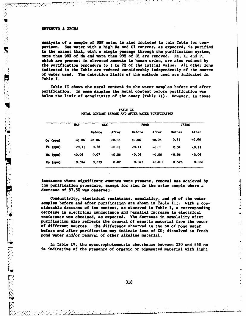
DEVENUTO & ZEGNA
analysis of a sample of USP water is also included in this Table for cam-parison. Sea water with a high Ns and Cl content, as expected, is purifiedto the extent that, with a single passage through the purification system,more than 982 of Na and more than 99% of Cl are removed. Na, K, and P,which are present in elevated amounts in human urine, are also reduced bythe purification procedure to 1 to 2% of the initial value. All other ionsindicated in the Table are reduced considerably independently of the sourceof water used. The detection limits of the methods used are indicated in
* Table I.
Table 11 shows the metal content in the water samples before and afterpurification. In some samples the metal content before purification wasbelow the limit of sensitivity of the assay (Table II). However, in those
TABLE IMTAL CONTENT BEFORE AND AFTER WATER PURIFICATIONX
US? SEA POND URINE
Before After Before After Before After
Cu (pp.) <0.06 <0.06 <0.06 <0.06 <0.06 0.71 '0.06
To (pp.) <0.11 0.38 (0.11 <0.11 <0.11 0.34 <0.II
Mh (pPM) 40.06 0.07 <0.06 '0.06 <0.06 <0.06 <0.06
Ze (PPM) 0.024 0.059 0.02 0.043 <0.011 0.526 0.066
instances where significant amounts were present, removal was achieved bythe purification procedure, except for zinc in the urine sample where adecrease of 87.5% was observed.
Conductivity, electrical resistance, osmolality, and pH of the watersamples before and after purification are shown in Table III. With a con-siderable decrease of ion content, as observed in Table I, a correspondingdecrease in electrical conductance and parallel increase in electrical
U resistance was obtained, as expected. The decrease in osmolality afterpurification also reflects the removal of osmotic material from the waterof different sources. The difference observed in the pH of pond waterbefore and after purification may indicate loss of C02 dissolved in freshpond water and/or removal of other alkaline material.
In Table IV, the spectrophotometric absorbance between 220 and 650 nm
is indicative of the presence of organic or pigmented material with light
L 318
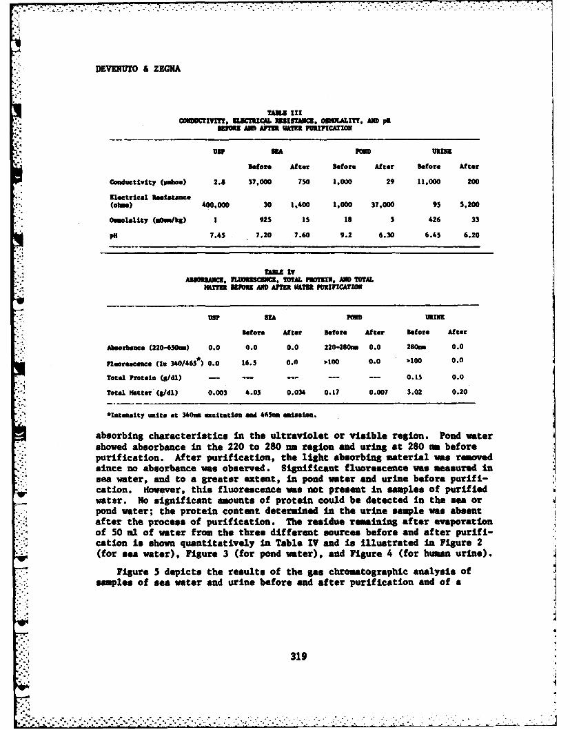
DEVENUTO &ZEGNA
TAML IIICUMIuPTIIT, BLUX CAL M3ISTMMC ONOULIT, MW PHE
ISa SEA I=U URINE
Before After Before After before After
Conductivity (wauos) 2.8 37,000 730 1.000 29 11,000 200
Electrical Resitance(ohmg) 400,000 30 1,400 1,000 37,000 93 5,200
Omiality (nu./ks) 1 925 Is 18 3 426 33
PHE 7.45 7.20 7.60 9.2 6.30 6.45 6.20
TAUX TVANSOMUNC, 1LUZCOIC, TOTAL PROTEIN, AND TOTAL
MATIER 331013 ANID AFTER WATER FURIV!CATZOU
US? SEA PMU URINE
Before After Before After Before After
Abeorbance (220-650m) 0.0 0.0 0.0 220-28Gmo 0.0 280nn 0.0
fluoceace (in 340,465 ) 0.0 16.3 0.0 2-100 0.0 )'100 0.0
Total Protein (/dIL) -- -- -- -- - 0.15 0.0
Total Mfatter (5/dl) 0.003 4.05 0.034 0.17 0.007 3.02 0.20
ftateneity units at 340=m excitation end 465iin inigeion.
absorbing characteristics In the ultraviolet or visible region. Pond watershoved absorbance in the 220 to 280 -a region and taring at 280 ta beforepurification. After purification, the light absorbing material was removedsince no absorbance was observed. Significant fluorescence was measured Insea water, and to a greater extent, in pond water and urine before purif 1-cation. However, this fluorescence was not present In samples of purifiedwatar. No significant amounts of protein could be detected in the sa orpond water; the protein content determined In the urine sample was absentafter the process of purification. The residue remining after evaporationof 50 ml of water from the three different sources before and after purifi-cation is shown quantitatively In Table IV and is illustrated in Figure 2(for sea water), Figure 3 (for pond water), and Figure 4 (for human urine).
* Figure 5 depicts the results of the gas chromatographic analysis ofsamples of sea water and urine before and after purification and of a
319
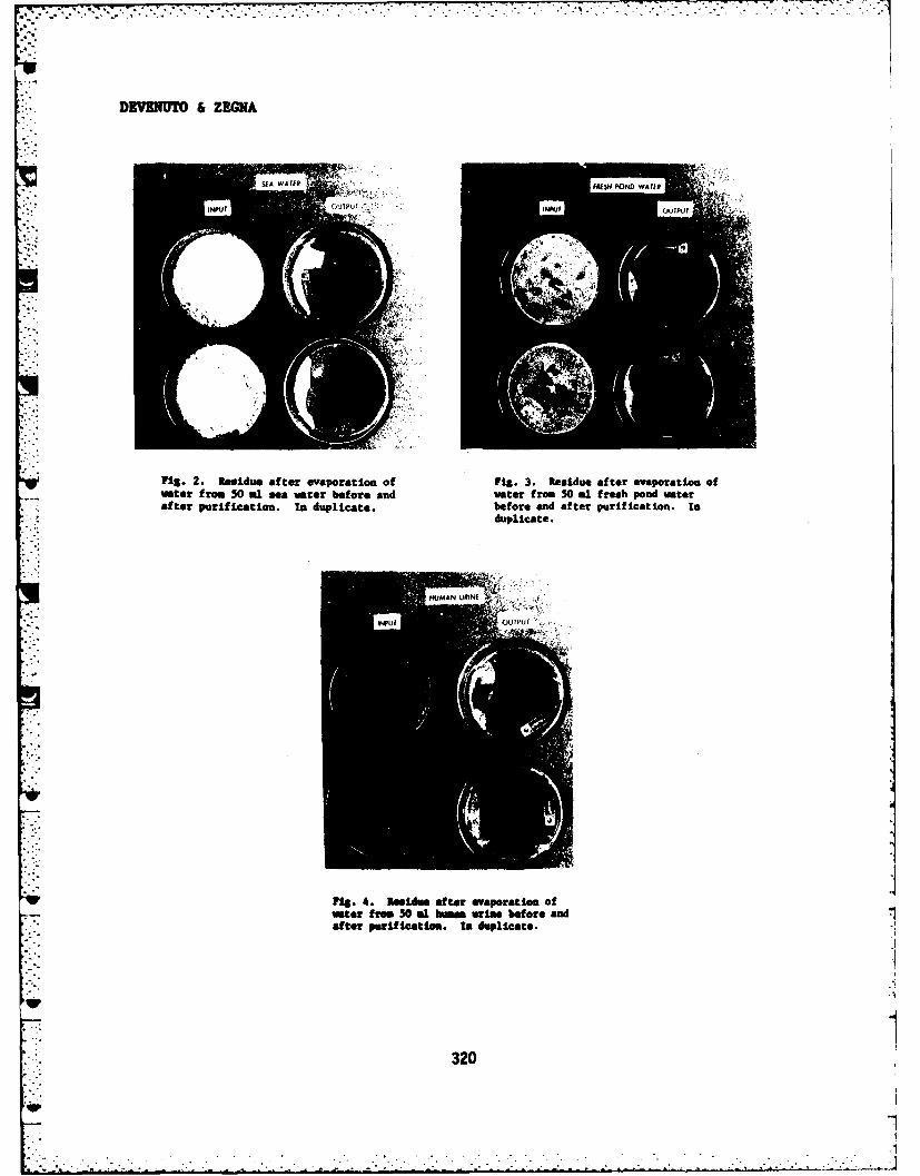
7lDEVh O & ZEGA
:
Fig. 2. Residue after evaporation of Fig. 3. Residue after evaporation of;ater from 50 al ea water before and water from SO al fresh pond water
* ater purification. in duplicate, before and after purification. Induplicate.
Fig. 4. residue after evaporation ofwater from SO al homes urine before and7after purificatiee. to duplicate.
320
eae rm5 lsawtrbfr n ae rmS lfehpn ae
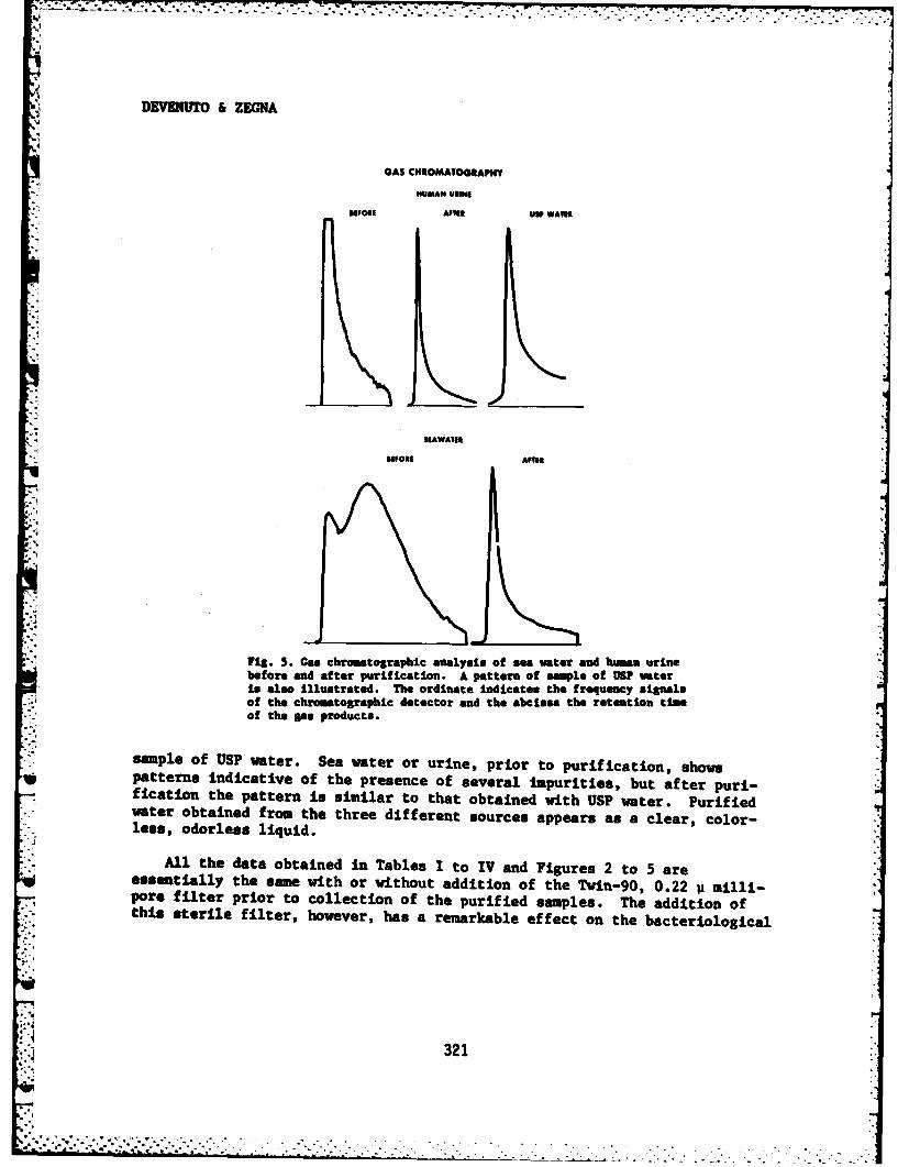
777 77 .7 7
DEVENUTO & ZEGNA
GAS CHROMATOGRAPHY
HUMAN yNMs
590ff1 AMRI UWP Whif
SEA WAIT
85011 AFN
Fig. 5.* Gas chroatographic analysis of sea water and human urinebefor, and after purification. A pattern of sample of US? wateris also Illustrated. The ordinate Indicates the frequency signalsof the chronatographic detector and the abcissa the retention tineof the gas products.
ample Of USP water. Sea water or urine, prior to Purification, showspatterns indicative of the presence of several impurities, but after puri-fication the pattern is similar to that obtained with US? water. Purified
* water obtained from the three different sources appears as a clear, color-loes, odorless liquid.
All the data obtained in Tables I to IV and Figures 2 to 5 areessentially the same with or without addition of the Twin-90, 0.22 ji milli-pore filter prior to collection of the purified samples. The addition ofthis sterile filter, however, has a remarkable effect on the bacteriological
321
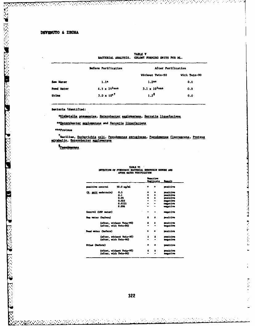
, . : .. . -. .o
. . . . .. .
.ACTERIAL ANALYSIS. COOY FOI G UNITS PER ML.
Before Purification After Purification
Without TvIn-90 With Tvin-90
Sea Water 1.1* 1.2** 0.0
POWd Water 4.5 x 10³** 3.1 x 10³**' 0.0
u Urine 3.0 x 1041 1.2# 0.0
Bacteria Identified:
Ae kbiebellm pneumonlae, Enterobacter aulomerane, Serratia liquefaciens
*'Eatero cter MuLnerana and Serratia liquefaciena
***Proteus
+Bacillus, Zecherichia col, Pseudomona aruginosa. Paeudomonas fluorescans, Proteus
m.rabi. Enterobacter M5 .!meran-". : PseudomonaaJ
TALE VIUTCTION OF F OGMIC RACIKMRL 3NOTOIIR M M
Ann YAMIIRIFICATION
ReactionDhaISCate Result
positive control 50.0 admni + + positive
(I. Ceoll eadotozin) 0.3 + + positive0.1 + + positive0.05 1 2 positive0.025 - namtive0.0125 - negative
"" " .006 negu~ative
Control (USP enter) cative
So water (before)t positive
(after. vitbut Twft-90) 1 * positive(after. with Ivin-90) negative
Pend water (before) + + positive
(after. without Win-90) 2 t positive(after, with Twin-o) - - negative
Urine (before) + + poiltive
(after. witheut Twin-90) * I positive(after, with Twin-") egative
322
_
DEVENUTO & ZEGNA
assays. The results of these tests are shown in Table V. Water obtainedfrom the three different sources is contaminated by different bacteria withvery heavy contamination observed in pond water and urine. Purificationwithout addition of the sterile filter shows little or no effect on theelimination of bacterial contamination from sea or pond water, althoughbacteria present in human urine are considerably reduced. However, theaddition of the sterile filter prior to collection of water assures absenceof bacterial contamination in the purified water.
Table VI shows the results of the detection of pyrogenic bacterialendotoxin in samples of water before and after purification. The limit ofsensitivity of the test is indicated by data of the positive control, re-presented by Escherichia coli endotoxin; this limit is reached at a con-centration of 0.05 ng/ml. Based on earlier assays, a pyrogenic response jwas obtained in rabbits at a concentration of 0.5 ng/ml. Prior to purifi-cation, water from the three different sources gave a positive reactionwhich is present also in purified water samples obtained without additionof a sterile filter. However, all the water samples collected after
filtration through the sterile filter show a negative reaction, indicatingremoval of pyrogenic bacterial endotoxin. A negative reaction was observedalso in the USP control water sample.
CONCLUSIONS
The data obtained in our studies demonstrate that the purificationsystem used satisfies all criteria for USP grade injectable water, exceptone: the limits of total solids. However, the purified water is non-
* pyrogenic, clear, colorless, odorless, and it is sterilized withoutaddition of antimicrobial agents or other substances. The ion, metal con-tent, and organic material present in human urine, pond water, and seawater are reduced considerably or completely removed by a single passagethrough the system. Although the total solids in the purified water exceedthe limit of 2 to 4 mgZ established for USP water, sodium and chlorine ions
," represent 96% and 64% of the total solids present in water purified from* sea water and urine, respectively. However, these ions are generally added
(900 mg sodium chloride per 100 ml) in order to make isotonic water forinjection. The results indicate also that organic substances, with spec-trophotometric absorption in the ultraviolet and visible regions, fluo-
U rescent compounds and protein material present in the water source areremoved by the purification process. It is important to emphasize thatthis purification system, as presently available, will not manufacturewater completely ste:ile and free of pyrogenic bacterial endotoxins, butrequires the addition of a small porosity, sterile, in-line filter to pro-duce water without bacterial contamination.
It appears that the reverse osmosis process is efficient in the pro-* duction of purified water and it has been utilized for the preparation of
323
pI
DEVENUTO & ZEGNA
drinking water in a desalinization project (8). The system evaluated inthese studies represents a multipurpose water purification process whichcould be useful in many non-military applications such as disaster siteswhere sources of water are contaminated, at construction sites, off-shoredrilling platforms, on commercial and pleasure boats, and other activitieswhere pure water is needed but not available.
REFERENCES
1. Dharan M: Standards and methods to obtain reagent grade water. LabManag 16:39-42, 1978.
2. The United States Pharmacopeia, USP Convention, Inc., Rockville, MD,19th revision, p. 540, 1975.
3. DeVenuto F, Moores WY, Zegna Al, Busse KR: Total and partial bloodexchange in the rat with hemoglobin prepared by crystallization.Transfusion 17:555-562, 1977.
4. DeVenuto F, Zegna Al, Busse KR: Lyophilization of crystalline hemo-globin solution and exchange transfusions with lyophilized-reconsti-tuted hemoglobin. Surg Gynecol Obstet 148:69-75, 1979.
5. DeVenuto F, Zuck TF, Zegna Al, Moores WY: Characteristics of stroma-free hemoglobin prepared by crystallization. J Lab Clin Med89:509-516, 1977.
6. Moore GL, Ledford ME, Brummell MR, Brooks DE: The potential use ofdihydroxyacetone for improved 2,3-DPG maintenance in red cell storage.Transfusion 20:24-31, 1980.
7. Valeri CR, Zaroulis CG% Rejuvenation and freezing of outdated storedhuman red cells. N Engl J Med 287:1307-1313, 1972.
, 8. Schmitt, RP: Military requirements for water supply. lirst Desalina-tion Congress of the American Continent 1:1-8 (V-2), 1976.
324
DUNN
A NEW ANALYSIS OF THE UNWINDING RIBBONAS A DELAYED ARMING DEVICE (U)
*WILLIAM P. DUNN, Ph.D.
US ARMY LARGE CALIBERWEAPON SYSTEMS LABORATORY
DOVER, NJ 07801
1. INTRODUCTION
The objective of this work was to formulate theoretical methods toenable engineers to design unwinding ribbons for use as delay armingmechanisms with reasonable accuracy and a minimum development effort.The unwinding ribbon considered here is a "wrapped" spring, which is aspiral spring made from flat metal stock closely wound. In the unstress-ed condition all the coils of the spring are touching. The results of theanalysis are given and compared with the experimental results obtained byT.B. Alfriend*.
This is a more complete study than that of Alfriend since no assump-tions are made concerning the moment of inertia of the coil and hub or
" the tension force in the ribbon bridge. Hence, two empirical constants in.. Alfriend's analysis were dropped in favor of exact expressions.
2. DESCRIPTION OF UNWINDER DEVICE
The basic components of the Unwinder device are shown schematicallyin Figure 1. The spring, A, iswrapped around and fastened at itsinner end to the shaft, B. The outer end of the spring is fastened tothe outer case, C, at the point D. The outer case, C, is fixed to androtates with the projectile. The axis of the spring and of the innershaft, B, are coincident with the longitudinal axis of the projectile
Uas shown in Figure 1. Upon firing, torsional acceleration causes the
spring to wind up tightly. After the torsional acceleration ceases, thecentrifugal forces acting on the spring will tend to unwind it. Duringthis unwinding process, the inner shaft, B, will rotate relative to thehousing, and this motion can be used to close a switch, to rotate a fir-ing pin in line with a detonator or to cause other arming processes.
*'Study of Wrapped Springs for Application to a Delayed Arming Device"-T.B. Aifriend -Summary Report ER-1404 Aircraft Armaments Inc.-1958.
325
.-s. a..,. .,-...... .......... ,.................... .. .. ........ •

L' ~ ~~~~~~~~~~ ~ ~~~~~ . .. ' ., , . ,. . ,.- -. .- ,, , - '. . -.. -. . - - - .- . . . . ' -. . -' ". -- - .-.- . -
DUNN
3. ALFRIEND'S ANALYSIS
To write the differential equation of motion of the spring unwindingdue to the action of centrifugal forces, Alfriend* assumed that the un-balanced torque on the nner shaft is a function of MI, where W is thenet angular velocity of the unbalanced spring mass and K is some experi-mentally determined constant. Pictorially, Alfriend represented the physi-cal problem as shown in Figure 2.
The internal force vectors L and are such that
.= the torque required to deflect the spring statically from itsinitial unstressed state with radius r , to the radius of theouter case, o, ;
£ = the tensile force in the spring due to centrifugal forces actingon the unbalanced length of the spring between points A and B,which are the points of contact between the stretched and coiledspring material at the inner and outer coils, respectively. Theinitial positions of these points are designated AS and 56
The appropriate Euler differential equation of motion for the inner shaftand attached spring is then
where * is the relative angular displacement of the shaft with respect tothe outer case. The moment of inertia, I, of the total revolving mass onthe inner shaft is a function of the radius, p , which decreases as thespring unwinds. Alfriend assumed
:,, IuZ ce (2)
where,
-= the initial moment of inertia of the spring plus the inner shaft
C - assumed constant rate of decrease in I as the spring unwinds.Alfriend then assumed
"(3)
* . *See reference in Introduction.
3261326',,': 2
.4 2', °','. .:. , :' ''' .'' ., '' . . - .' _ .,- - • / ' _.: , i ,. - , _ , ; : -, "; ." "-. -" "

DUNN
where as aforementioned, is experimentally determined and do is thetotal angular velocity of the unbalanced spring length. He furtherassumed that
0) X .u a (4)
where,
ru,-I (5)
and,
- constant angular velocity of the outer case
- spring thickness
e = initial outside radius of the spring on the inner shaft.
Substituting equations (2) - (5) into (1), the equation of motionbecomes
where,
(6-A)
and,
E - the elastic modulus (Young's) of the spring material
b - the width of the spring material
the radius of the inner shaft
the radius of the outer case
4. MODIFIED ALFRIEND THEORY
A more accurate characterization of the behavior of the spring can beobtained by eliminating the assumptions made by Alfriend. To accomplishthis, equations (2) and (3) are replaced by their analytically derivedforms. This eliminates the two constants M and 6 introduced through theassumptions; in place of equation (2),
327

DUNN
%f4&-r)XA j (7)
where3 lop , are the inner shaft and spring densities, respectively.
To revise equation (3), consider Newton's 2nd Law of Motion i.e,,the force is proportional to the change in momentum with time. and let
'Ir u mass of the spring material between
points "A" and "B" in Figure 3 (8)
-,W - (.' +wr) a the position vector to the center of mass ofmaterial between the points "A" and "B" inFigure 3 (9)
"the velocity vector of the mass center ofthe material between the points "A" and "B"in Figure 3 (10)
where
r a the position vector to the last point of contact between theinner coiled spring material and the uncoiled springmaterial =( o. X "0 )('wmJ'9 e (1)
-X V the position vector to the last point of contact between the,_outer coiled spring material and the uncoiled spring material
and
- the initial radius of the last point of contact between the innercoiled spring and the uncoiled spring.
t= the inner radius to the outer case
S- the angle delineating the material unwrapped from the inner core
at- the angle delineating the material wrapped onto the outer case
"angk-,between the position vector rjand the uncoiled material -
r the scalar value of i r. (*A.)* (13)
328
-, S . ~ \ * .---- ' -* -". . . . . .:

DUNN
DN athe scalar value of )~a~~C u~(14)
Thus, the force acting on the ribbon segment ( ) is,
FNje s~j4 w re (15)
where,
(16-A)
and in place of equation (6-A), we define
(16-B)
The transformation expressions relating the coordinate system fixed in
the inner shaft to the ground reference coordinate system are:66 4 4
W 2"-t~Z~s ji*' L
(17)
Substituting 64 1 (18)
Substituting equations (17) into equations (9), (10) and dEQ/Jt yields,upon simplification,
revfft0Cra rmi iJ (19)6n" €.r(fJ.. (im jr$ Vj- * (~,JJX)
J T (21)
.
329
h,,;,",,,. ,;,,,-: . ..-.- ,-, .- ,....- -.-. .-... .-. ,.... .. .. .-.... .- ,. . . .

DUNN
Def ining,
T .,3(22)
and noting from Figure (3) that
-,,P (23)
differentiation then provides the relations
0 4id u • (24)
Now, using equations (18) or (20) and (21); along with equations (22),(23) and (24), obtain from equation (15)
FW VPr&C Cj-A ' 121 8 1 a
*.-.: *t [r LJ -JII. S Crh.,X -q.
ta "
w
fE~±~4 A WD
vetr a resetiey From Figur 3, the teso in thesegen
FLI-r q AL- a s (26)
Substituting 15 and 4 from equation (25) into (26) and making use of the
trigonometric identities
cbfru *0p)= 8., ; %W'r wO (27)
330
"330
/;4 , ,
DUNN
yields, upon simplification,Fv 4,t, A '04 a .:: F- -q tP-,, K's" -- J w '7
£11 J ~ (28)
After substituting (See Figure 3),
S - ,(29)
into equation (28) and then using this result in equation (1), thefollowing expression is obtained.
- ( i~aci.4r. ofj(.(~7-i) (30)
where,::'::A 2 " m (31)
for the case
5. RELATIONSHIP BETWEEN WRAPPING ANGLE (09) AND UNWRAPPING ANGLE (8):
To obtain ag as a function of 0 , note from Figure 3 that the materialunwrapped from the inner shaft must equal the material wrapped on the outercase plus the material going into the increased length of the "bridge",Matbmat ically stated,
Substituting equations (13) and (14) into equation (32) and integratingyields,
(r-A4 (33)
Expanding and simplifying equation (33) results in
331

o.
DUNN
j a
6. DETERMINATION OF MAXIMUM WRAPPING AND UNWRAPPING ANGLES:
It can be seen from equation (13) and Figure 3 that the minimum valueof r, t', will yield the maximum value of ; i.e.
4,45.-U .- ,.) (35)
The maximum wrapping angle is found by noting that
Rearranging terms and squaring the radical leads to
Neglecting terms containing S , a first approximation for equation (36)produces
-o (37)
A final approximation can be made if Lare*)D/. . That is,
+ ", (38)
7. DETERMINATION OF r., THE INITIAL OUTSIDE RADIUS
If /.,0, 4 and IS are given, f is obtained by first noting that thecoil length, / can also be determined from -
Pit +I. r (Ps 0z+ ",'
332

DUNN
Rearranging terms and squaring the radical then yields
.ii P 'O(39)
To obtain a real solution to equation (39), it is required that
fS*' '. (40)
which is obtained by imposing the condition that the radical term in
__p: (41)
be real. Taking the positive sign in equation (41) to insure a real root,provides the relation
$4J tj* (42)
8. ALGEBRAIC SIMPLIFICATION OF THE EQUATION OF MOTION (Equation (30))
For the following conditions:
equation (33) provides the relationship
":"(43)
Substituting equation (43) into equation (22) results in
at (44)
Thus, using equation (44) and taking the time derivative of equation (22)
3331
"'" 333

DUNN
.y differentiating equations (13) and (14) the following time derivativerelations are obtained:
) .. f...(46)Hence, from equations (45) and (46),
r 1 ~.reuo(47)
and,
& 0. kid(48)
Substituting equations (46), (47) and (48) back into equation (30),simplifying and rearranging yields
".0+,40 A-Asi +Ai o (49)
where,
As*
* A.(~.)'t,/A,(50)A,-A-J - /w
AOR SAIie .,
These equations together with the initial valves,
ft..I2 G(too).o , eA9 (51) r
completely define the unwrapping angle as a function of time.
334]
";:1, ...', "..'.'-- ",':'-i-'-' ' -'.-'--..... . .. . . . .. . . . ."' "- ", . -. ,-.
DUNN
9. EXPERIMENTAL PARAMETERS
To evaluate equation (49) for its accuracy in predicting the armingtime of an unwinder fuze, a comparison is made between Alfriend's experi-mental test data and the analytic results. The parameters for Alfriend'sexperiments are given in Table 1.
10. RESULTS, CONCLUSIONS AND DISCUSSION
Analytic and experimental results are plotted in Figures 4 through 10.Surveying these results, it is found that springs 1, 3, 4, 6 and 7 providea good correspondence between theory and experiment, with the correlationbecoming increasingly better as the angular velocity of the outer caseincreases. The poorest theoretical-experimental correspondence occurs withsprings 2 and 5, although the trend of the relative turns versus time datawith increasing outer case spin is predicted.
It is interesting to note that the fall-off of experimental data pointsfrom analytically determined points in spring 5 (at a relatively high outercase spin) appears similar to that. for the lowest outer case spin rate forspring 1.
Without a thorough knowledge of experimental procedures, devices anddata, the reasons for differences between experimental and analytic resultscannot rationally be examined. How well the mathematical model will describethe results of an experiment depends on how well the experimental set-up istrue to the conditions of the mathematical model. Since the data used inthis report must be taken and used as reported, the reason(s) for the dis-crepencies between analytic and experimental results was not sought.
335
. .,. - .. -- -. *- .- .... -. - -o - -. . . .... . .. .. . .. . .. .)o .. , ° % °, " . . . , • . . o.C.,' . o' o. -' . ° - ° o . . • . o -. . ° . . . •
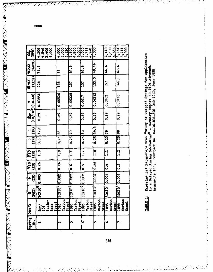
DUNN
NCOt 00 00%Go -4 o % r- 0%
- a-A
0%
-4 4 - -4 - P-4r4-4
$44r
C; 04
z 0
H e'" 0 al 0 NC4 C4 e C$
'-0 0 M
-n r- 10 'GoN N
' a N-4P! C
1O.4
100
C4 0 m 41 % w .0(IN 4 6P0 ~ ~~ N -i NuJ$
S4 4l - ~ 0cOscaP04,1 Io-Ic v2 a
N4 en An N %4 i P
0 0 0 0 336
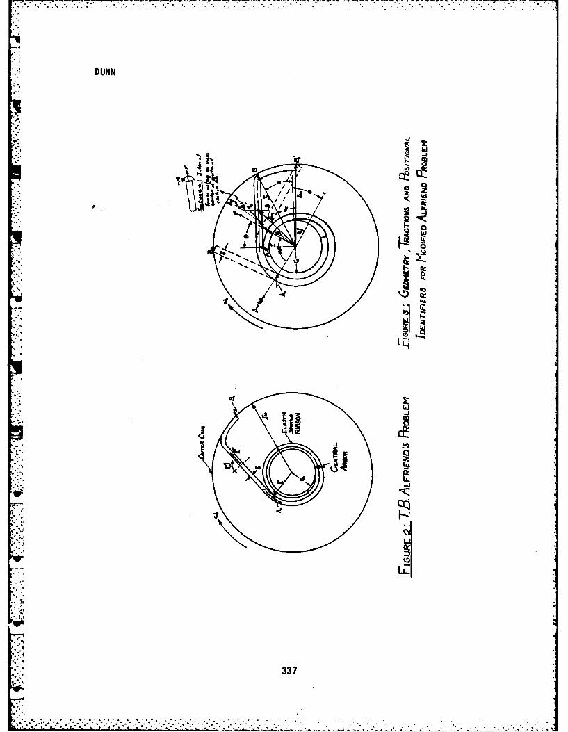
DUNN
'Ij
-I
T337
U"A
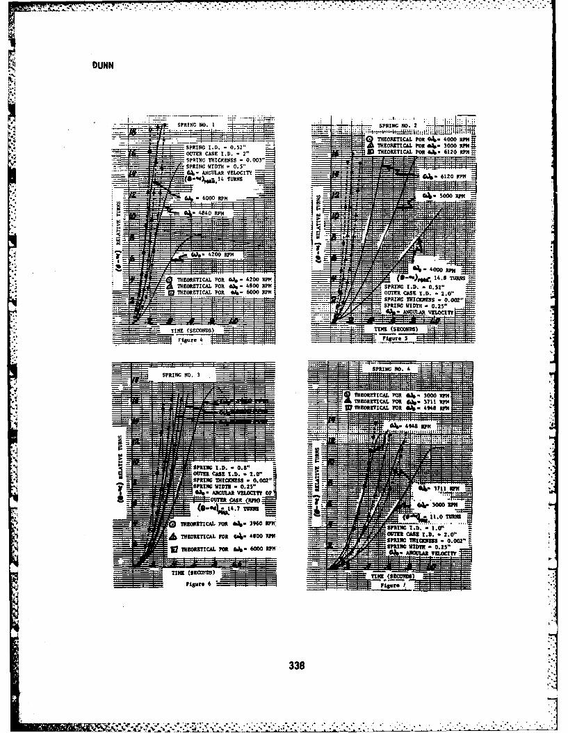
. . .-~~~~ .. . .- . . . - . . . . . .
DUNN
SPRING 1.0. -0.52" THEORETICAL FOR d4- 3000 RPM~OUTER CASE I.0. , 2" THEORETICAL FOR &J~6120 RPM
SPRINTHIC K_ FOR n. 4200 - -4 -UII
SPHEREICAG WIOR - 000R.5"E AS .. .
AIE(SCNGULA VELOCITTEYSECUDS
THEORETICAL FOR We - 400 RPM41. UN
THEORETICAL FO ah - 4800 RPM -SPRING mom - 0.2"
THORTIALFR 4-600RP OTE CS338.- .
~~SRN . . . . . . . . . . . . .
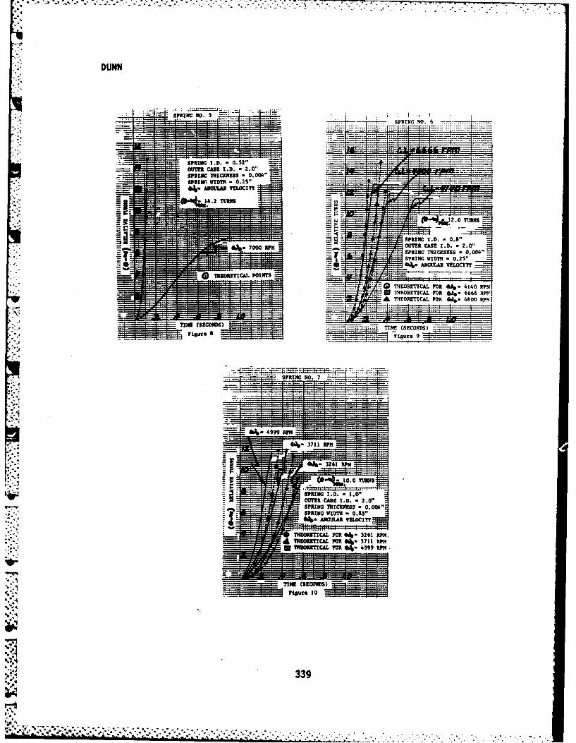
DUNN
- stRUE c No . 0 S2
6- ANUA v IU =
CASE ISECO-D2.0"
THOEIA FORur 464 410 1M
THERETCA FO *-666R
33OEIALFR9- 80RM
70 (SCND)TME(ECNS
DUTHIE, ASHLEY, UPATNIEKS & LIU
PHOTONIC SEEKER DEVELOPMENT (U)
*JOSEPH G. DUTHIE, DR., PAUL R. ASHLEY, DR.RESEARCH DIRECTORATE, US ARMY MISSILE LABORATORY
US ARMY MISSILE COMMANDREDSTONE ARSENAL, ALABAMA 35898
ANDJURIS UPATNIEKS, MR.** AND H. K. LIU, DR.***
INTRODUCTION
Ideally, a seeker system to be used for target identification and mis-sile guidance should be able to recognize the target over an extended setof ranges, orientations and aspects. In the most simple scenario a singlefeature such as a characteristic infrared emission or designation of thetarget by an aimed laser spot will suffice. However, for autonomous seekewhich have to seek out and destroy energy targets without the aid of laserdesignators or where the differentiation between friend or foe is moredifficult, far more information has to be processed than ay be possible byelectronic means.
Consider the problem of identifying and correctly locating a single.3 scale, orientation and aspect of an enemy vehicle in a snapshot taken with
a typical instamatic camera. For this example we will take the focallength of-the lens to be 2 cm, the lens aperture to be 1 cm, the wavelengthof the light to be 5 x 10- cm and the field of view 1 cm x 1 cm. Thenumbers are useful only for order of magnitude calculation and need not re-present an actul system. In the image plane the size of the rfsoluttonelements is 10" ca. Thus, the image may be thought of as a 10 x 10' arrayof resolvable elements. To recognize and locate the tank, the optimumestimator can be shown to be the cross correlation between a known bmge ofthe tank and the image to be searched. For an image consixting of 10qx 10 q '
resolvable points, this involves computing two separate 10 x 104 pointFourier Transforms, mnltiplying the two together then forming be 10 x 104point Fourier Transform of the resultant. A total of about 10 aultipli-catione is Involved. The task of doing this at T.V. frame rates requires
** Permanent Address: n x Michigan0.' gm• n r or,1*** Permanent Address: University of Alabama, Tuscaloosa, AL 35486
.1 341 .. .. . .
DUTHIE, ASHLEY, UPATNIEKS & LIUp 4
about 1012 multiplications per second and is well beyond the capability ofany digital computer. Of course one could relax the requirements consider-ably in terms of number of resolution elements or processing rate, but only
at the cost of reduced performance.
The photonic correlator, however, has such a capability today. It has
the added advantages of low power consumption, mechanical simplicity and it
can be made mall enough to fit comfortably into a submissile. There are,
however, several limitations which must be overcome before the use of
photonic correlators become a reality for missile systems. These include
the cost of the light modulator and the need for extending the memory of
the photonic correlator to include an extended set of target scales, sizes
and orientations. The problem of cost for the light modular appears to be
one of manufacturing techniques and it should be possible to produce low
cost devices cheaply enough in suitable quantities. The need to extend the
memory of the correlator has been the subject of much of our recent re-search on the use of photonic correlators.
The MICCM. Photonic Correlator - An Overview
The science of photonic optical information processing relies heavilyon the Fourier Transforming Properties of Lenses (1). This was applied byA. B. Vander Lugt of the University of Michigan's Radar Laboratory, who,in 1963, demonstrated a new technique for synthesizing matched filters forcoherent processors (2) (3).
Figure 1 represents the two stages of coherent image processing usingVander Lugt filtering techniques. In Figure 1A, a reference scene on atransparency of amplitude transmittance (x,y) is illuminated by a source ofcoherent light. The transparency is in the front focal plane of the FourierTransforming lens L1. In the back focal plane is located a photographicplate. Exposure of the plate to the transformed image (x,y) simultaneouslywith a reference beam produces what is called a matched spatial filter ofthe reference scene. Subsequent to development, the plate is re-insertedin the optical system as in Figure 1B. In this case the reference beam is
* ~ removed and a new input transparency S(x,y) is inserted. The property ofthe matched filter is that in the arrangement shown in Figure 1B, the de-tected output n the cross correlation of f(x,y) and g(xy), i.e., a brightspot will appear in the output plane if g(x,y) contains sufficient infor-matton about f(xy). Furthermore, the position of the spot is a functionof the position of the object located in S(x,y). Thus, the photonic corre-lator can effectively detect the presence of a test object in a given fieldof view.
As an example of the technique Figure 2 shows an image of a sedan usedto make a Vander Lugt filter for the photonic correlator. Figure 3 showsthe respose of the correlator to a series of scenes showing the same
342
,."q
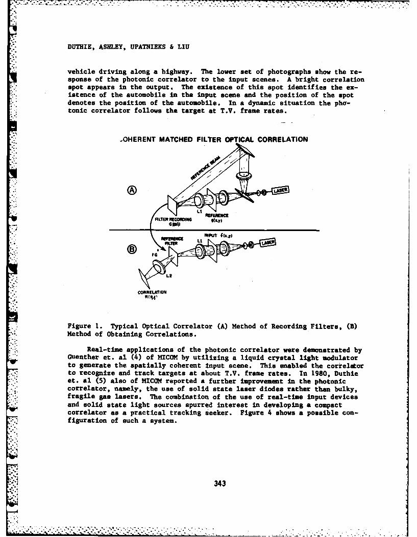
DUTHIE, ASHLEY, UPATNIEKS & LIU
vehicle driving along a highway. The lower aet of photographs show the re-sponse of the photonic correlator to the input scenes. A bright correlationspot appears in the output. The existence of this spot identifies the ex-istence of the automobile n the input scene and the position of the spotdenotes the position of the automobile. In a dynamic situation the pho-tonic correlator follows the target at T.V. frame rates.
"OHERENT MATCHED FILTER OPTICAL CORRELATION
- 'FILTER REORIG
"" CORRELATION
Figure 1. Typical Optical Correlator (A) Method of Recording Filters, (B)Method of Obtaining Correlations.
Real-time applications of the photonic correlator were demonstrated byGuenther et. al (4) of MICOM by utilizing a liquid crystal light modulatorto generate the spatially coherent input scene. This enabled the correlatorto recognize and track targets at about T.V. frame rates. In 1980, Duthieet. al (5) also of MICOM reported a further improvement in the photoniccorrelator, namely, the use of solid state laser diodes rather than bulky,fragile gas lasers. The combination of the use of real-time input devicesand solid state light sources spurred interest in developing a compactcorrelator as a practical tracking seeker. Figure 4 shows a possible con-figuration of such a system.
*343
-.- :,~ Z ::~ -.. .,.... . . - .
- DUTHIE, ASHLEY, UPATNIEKS & LIU
Figure 2. Example of Correlator Input (a) Input Object (b) Matched Filter
of some Object.
Increased Memory for the Photonic Correlator
Major improvements need to be made in the capacity of a photonic cor-relator to store and address a large number of reference images before thephotonc correlator can be regarded as a serious contender for missileguidance and tactical homing applications. Leib et. al (6) have designedan optical matched filter correlation system in which a large array ofholograms can be stored in a matched filter through the use of a multiplenumber of holographic lenses. Theoretical predictions of a capability tostore up to 2500 matched filters have yet to be realized in the laboratory.
4.A new method of addressing an array of matched filters has been de-veloped by Liu and Duthie (7) at MICOM. In the basic correlator system of
* Figure 1, a phase screen is placed n the input plane. This screen hashigh optical transparency but spatially modulates the phase of the lightwaves. The periodic modulation is chosen so as to generate an array ofIslands n the Fourier Transform plane of the correlator. Figure 5 showsa photomicrograph of the phase screen while Figure 6 shows the array ofislands found n the transform plane. Thus, the effect of the phase screen
.4 344
C.. .. . C . ...
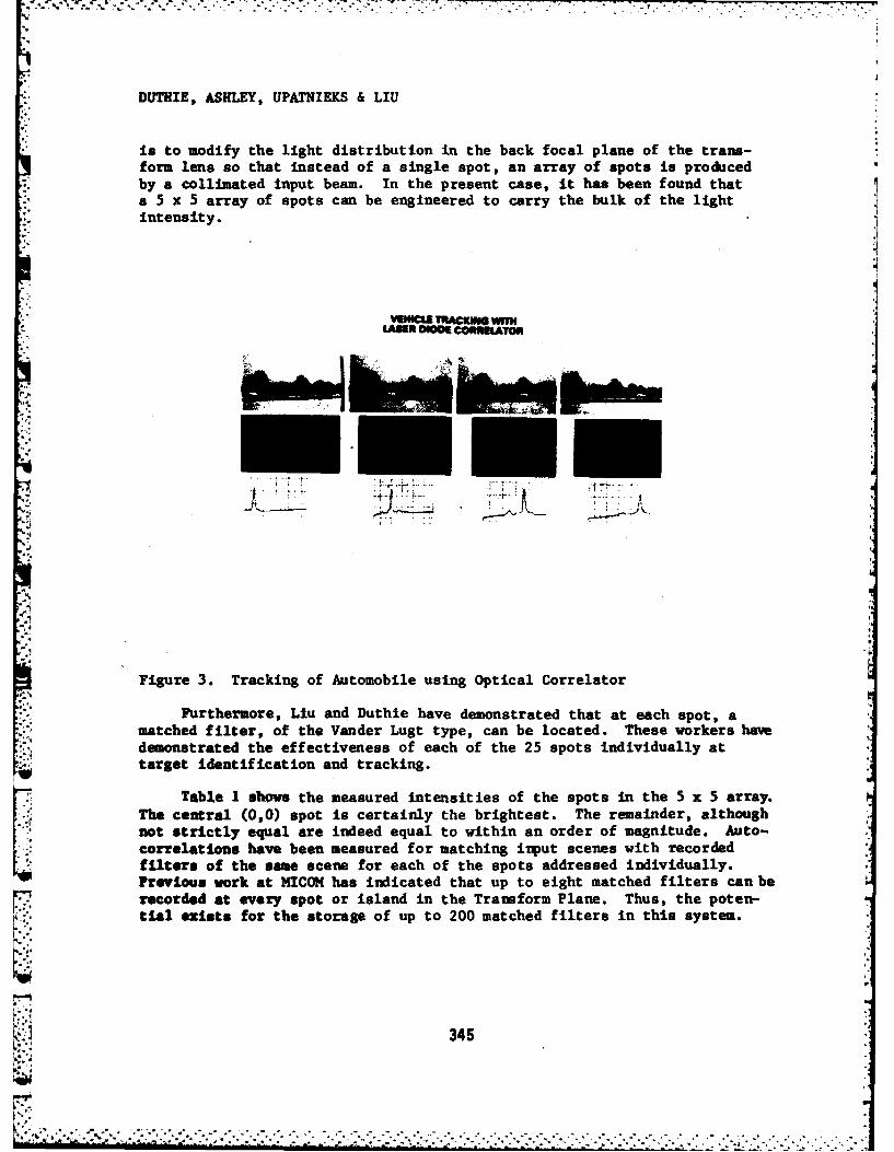
DUTHIE, ASHLEY, UPATNIEKS & LIU
is to modify the light distribution in the back focal plane of the trans-form lens so that instead of a single spot, an array of spots is producedby a collimated input beam. In the present case, it has been found thata 5 x 5 array of spots can be engineered to carry the bulk of the lightintensity. j
LAW1R DOMS confamM
mathe fitr fteVneuttpca elctd hs okr a-- U-
Figure 3. Tracking of Automobile using Optical Correlator *
Furthermore, Liui and Duthie have demonstrated that at each spot, amatched filter, of the Vander Lugt type, can be located. These workers have
demonstrated the effectiveness of each of the 25 spots individually attarget identification and tracking.
Table 1 shows the measured intensities of the spots in the 5 x 5 array.The central (0,0) spot is certainly the brightest. The remainder, althoughnot strictly equal are indeed equal to within an order of magnitude. Auto-correlations have been measured for matching input scenes with recordedfilters of the same scene for each of the spots addressed individually.Previous work at MICOM has indicated that up to eight matched filters can berecorded at every spot or island in the Transform Plane. Thus, the poten-tial exists for the storage of up to 200 matched filters in this system.
I..346K.7
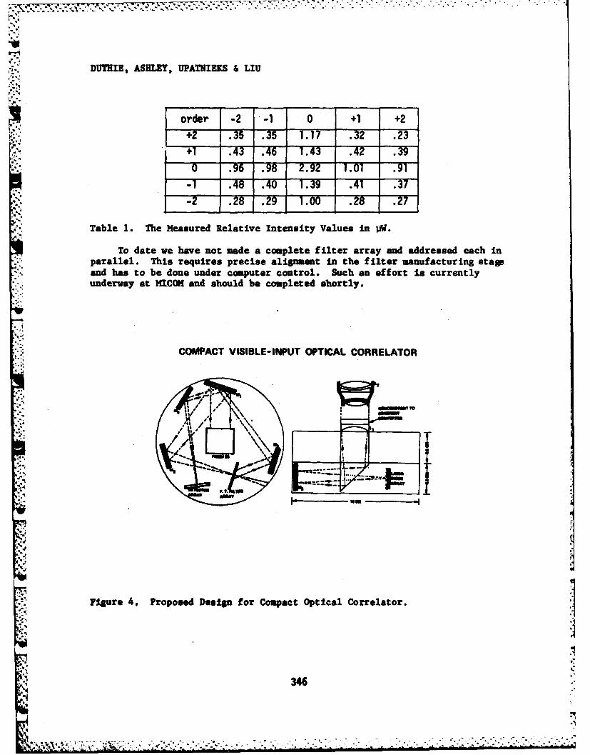
DUTHIE, ASHLEY, UPATNIEKS & LIU
order -2 -1 0 +1 +2.-1 .3 35 5 3 1.17 .32 .23
.. )+1 . 3 .46 1T.4 - -. 4T - -. 39
W0 .96 .98 2.92 1.01 .91
r 1 .48 .0 .39 .41- .37.,,-2 .28- .2v9 1.0O0 .28 .7
Table 1. The Measured Relative Intensity Values in W.
To date we have not made a complete filter array and addressed each inparallel. This requires precise alignment in the filter manufacturing stageand has to be done under computer control. Such an effort is currentlyunderway at MICOK and should be completed shortly.
*". COMPACT VISIBLE-INPUT OPTICAL CORRELATOR
4*0
346
N:- : , .,' '': " r , :: " . . . , . o ' , . . . . .. ' . o . -
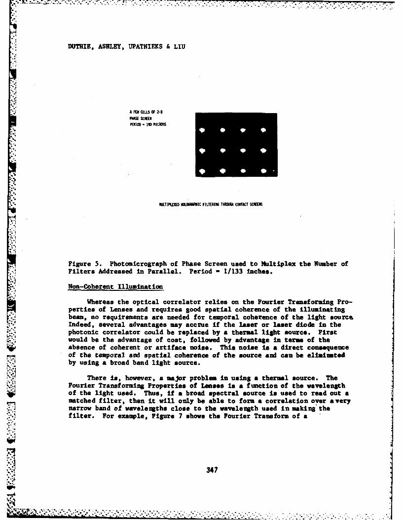
DUTHIE, ASHLEY, UPATNIEKS & LIU
A FEW CELLS OF 2-0
PHASE SCRENPERIOD - 190 MICRONS
FKTIPLEX1 HO06 IC FILTERING THROUGH CONTACT SCREENS
Figure 5. Photomicrograph of Phase Screen used to Multiplex the Number of
Filters Addressed in Parallel. Period - 1/133 inches.
Non-Coherent Illumination
Whereas the optical correlator relies on the Fourier Transforming Pro-perties of Lenses and requires good spatial coherence of the illuminating
. beam, no requirements are needed for temporal coherence of the light sourceIndeed, several advantages may accrue if the laser or laser diode In thephotonic correlator could be replaced by a thermal light source. Firstwould be the advantage of cost, followed by advantage in terms of theabsence of coherent or artiface noise. This noise is a direct consequenceof the temporal and spatial coherence of the source and can be eliminatedby using a broad band light source.
There is, however, a major problem in using a thermal source. TheFourier Transforming Properties of Lenses is a function of the wavelengthof the light used. Thus, If a broad spectral source is used to read out amatched filter, then it will only be able to form a correlation over averynarrow band of wavelergths close to the wavelength used in making thefilter. For example, Figure 7 shows the Fourier Transform of a
347
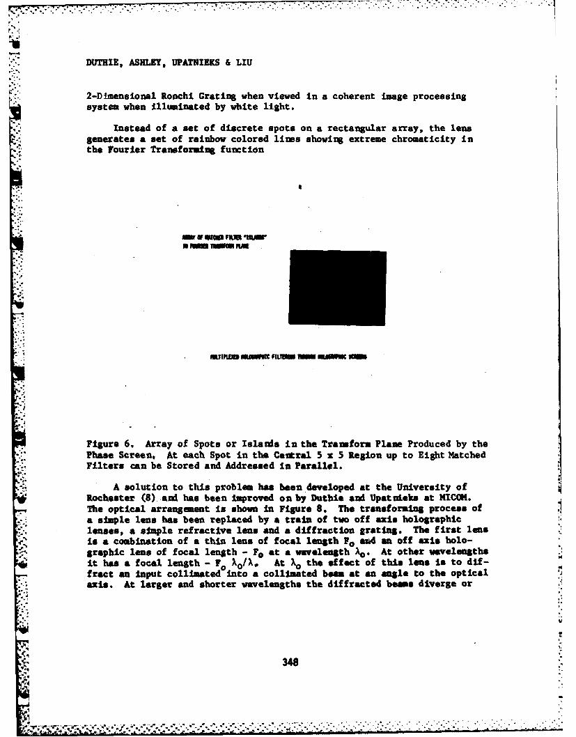
4. DUTHIE, ASHLEY, UPAflIIEKS &LIU
* .. ,2-Dimensional Ronchi Grating vhen viewed in a coherent image processingsystem when Illuminated by white light.
Instead of a set of discrete spots on a rectangular array, the lensgenerates a set of rainbow colored lines showing extreme chromaticity inthe Fourier Transforming function
MW wa WFLM ImwIINUU i RM
WIREU NOMUC FILl" W AA WONC
Figure 6. Array of Spots or Islatls in the Transform Plane Produced by thePhase Screen, At each Spot in the Ceitral 5 % 5 Region up to Eight MatchedFilters can be Stored and Addressed In Parallel.
* A solution to this problem has been developed at the University ofRochester (8) and has been Improved on by Duthie and Upatnieks at )flC(I.The optical arrangement is shown In Figure 8, The transforming process ofa simple lens has been replaced by a train of two off axis holographiclenses, a simple refractive lens and a diffraction grating. The first lensis a combination of a thin lens of focal length P0 and en off axis holo-graphic lens of focal length - F0 at a wavelength Ao. At other wavelengthsit has a focal length - F0 XO/X At X0 the effect of this lens is to dif-fract an Input collimated Into a collimated bean at an angle to the opticalaxis. At larger and shorter wavelengths the diffracted beams diverge or
348
DUTHIE, ASHLEY, UPATNIEKS & LIU
Figure 7. Conventional WhiteLight Fourier Transform of a2-Dimensional Ronchi Grating.Note the Extended Nature ofthe Individual Orders due toSevere Chromatic Effects.
rjEOfETRY AF OPTICAL SYSTEI TO 1EIERATE ACHRfV TIC Ft).IEQ TRAISMPIS
Figure 8. Optical Arrangement for Achromatic Fourier Transform System.
349
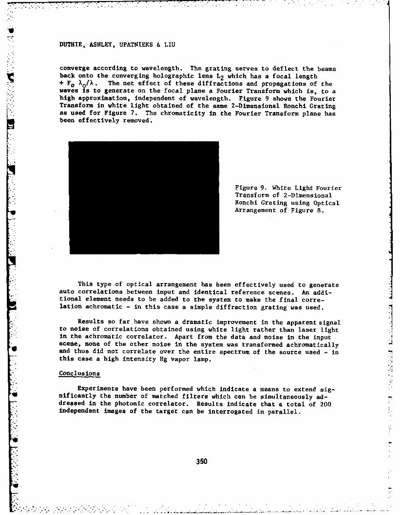
DUTHIE, ASHLEY, UPATNIEKS & LIU
converge according to wavelength. The grating serves to deflect the beamsback onto the converging holographic lens L2 which has a focal length+ Fo A. The net effect of these diffractions and propagations of thewaves Is to generate on the focal plane a Fourier Transform which is, to ahigh approximation, independent of wavelength. Figure 9 shows the FourierTransform in white light obtained of the same 2-Dimensional Ronchi Gratingas used for Figure 7. The chromaticity in the Fourier Transform plane hasbeen effectively removed.
Figure 9. White Light FourierTransform of 2-DimensionalRonchi Grating using OpticalArrangement of Figure 8.
This type of optical arrangement has been effectively used to generateauto correlations between input and identical reference scenes. An addi-tional element needs to be added to the system to make the final corre-lation achromatic - in this case a simple diffraction grating was used.
Results so far have shown a dramatic improvement in the apparent signalto noise of correlations obtained using white light rather than laser lightin the achromatic correlator. Apart from the data and noise in the inputscette, none of the other noise in the system was transformed achromatically
* and thus did not correlate over the entire spectrum of the source used - inthis case a high intensity Hg vapor lamp.
Conclusions
Experiments have been performed which indicate a means to extend sig-*i nificantly the number of matched filters which can be simultaneously ad-
dressed in the photonic correlator. Results indicate that a total of 200independent images of the target can be interrogated in parallel.
350
DUTHIE, ASHLEY, UPATNIEKS & LIU
This corresponds to an effective computation of over 1013 complex multi-plications per second. The suggested method is mechanically simple, op-tically easy to implement, requires little power and can be fabricated intoa compact unit.
Improvement in the signal to noise of a photonic correlator can beachieved by using an achromatic transform system and a thermal light source.At this time, however, the throughput of such a system is not sufficient tomake a practical device. Whereas, efforts should continue to develop tech-niques to correlate using thermal light sources, the principal thrust formaking a field operational system should, at this time, be concentrated onthe use of laser diode sources together with the use of phase screens toextend the memory of these systems.
REFERENCES
1. See for Example, J. W. Goodman, "Introduction to Fourier Optics",McGraw-Hill, (1968).
2. A. B. Vander Lugt, "Signal Detection by Complex Spatial Filtering",Radar Lab Report 4594-22-T, (1963).
3. A. B. Vander Lugt, "Signal Detection by Complex Spatial Filtering",IEEE Trans. Inform. Theory, IT-10:2, (1964).
4. B. D. Guenther, C. R. Christensen and J. Upatnieks, "Coherent OpticalProcessing: Another Approach", IEEE J. Quantum Electronics, WE-15, 1348,(1979).
5. J. G. Duthie, J. Upatnieks, C. R. Christensen, and R. D. McKenzie,"Real Time Optical Correlation with Solid State Sources", SPIE 231, 281,(1980).
6. K. G. Leib, R. A. Bondurant, M. R. Wohlers, "Optical Matched Filterrorrelator Memory Techniques and Storage Capacity", Opt. Engr. 9, 414,(1980).
7. H. K. Liu and J. G. Duthie, "Real Time Screen Aided Multiple ImageOptical Holographic Matched Filter Correlator", submitted for publication,Applied Optics, 1982
8. G. M. Morris, "Diffraction Theory from Achromatic Fourier Transfor-mation", Appl. Opt. 11, 1255 (1972).
351
..
ELDER, WALBERT, ZIMMERMAN
TITLE: STATIONARY AND TRAVELING LOADS IN A HOLLOW CYLINDER
ALEXANDER S. ELDER, MR.JAMES N. WALBERT, DR.
KATHLEEN L. ZIMMERMAN, MRS.US ARMY BALLISTIC RESEARCH LABORATORY
ABERDEEN PROVING GROUND, MD 21005
I. INTRODUCTION
Just after World War II Dr. R. Beuwkes [1] of Watertown Arsenalintroduced the senior author to the theory of elastic stresses in thick-walled cylinders and the technology of shell-pushing tests. The researchat Watertown Arsenal culminated in the publication of the Thick WalledCylinder Handbook [2], a monument to skill in analysis and computations ona desk calculator. Investigation of non-metallic rotating bands at BRL ledto renewed interest in this area. We found that we were unable to inter-polate in the tables cited above due to their limited accuracy; moreoverthe value of Poisson's ratio used in the computations was not appropriatefor modern gun steels. An independent investigation was initiated, usingresidue theory in place of Fourier series [3,4,5]. Since the eigenvalueswere complex, we required a subroutine for Bessel functions of integralorder and complex argument. The required subroutine was developed at BRL.A Gauss continued fraction was used to reduce round off errors inherent inseries calculations [6,7]. A code giving accurate stresses on the outsideof the gun tube was developed [8,9]. This code was used to calculatestrains in a highly instrumented gun tube. The appropriate value ofPoisson's ratio and Young's modulus was obtained from the Benet Laboratory.Agreement between theory and measurement was good at low velocities, butsystematic deviations were observed at high velocities. This result wasforecast in an early paper by G.S. Taylor [10], who used a dynam:i versionof the Winkler theory for thin-walled tubes, but his results wereapparently ignored by the Army. A program based on scalar and vector wavefunctions was initiated at BRL. The computations are difficult except fortorsion, which we discuss below. The theoretical work shows that theequilibrium stress distribution is obtained when the velocity of travel- r approaches zero in the limit, as one would expect on physical grounds.
353* " . .
%
ELDER, WALBERT, ZIMMERMAN
Recently we have resolved difficulties in calculating stresses near adiscontinuity of loading on the inner surface of the cylinder. A method ofcalculating elastic stresses in thin-walled cylinders was also derived, sowe are able to use the same mathematical formulation for wall ratiosranging from .01 to S. Both of these problems required asymptotic methodsand involved large values of the complex transform variable in the analysis.
II. NUMERICAL DIFFICULTIES
Formulation of boundary value problems for the infinite hollowcylinder has followed traditional lines and is not exceptionally difficult.Real problems arise in the numerical evaluation of Fourier integrals andthe generation of Bessel functions of the second kind due to the integerarithmetic of the digital computer and its limited exponent range. Memoryrequirements and execution time are relatively modest for the class ofproblems under consideration. We have considered four types of error inthe course of programming and numerical analysis.
Round off error is persistent and insidious. It is very severe in theevaluation of Fourier integrals by quadratures along the real axis and wasthe principle reason why the calculus of residues was used in preference.It occurred in acute form in calculating Bessel functions of the secondkind. This difficulty motivated our development of the subroutine citedabove. In this paper we discuss round off error occurring in the manipu-lation of asymptotic series. Round off error is also a principle concernin generating special functions by recursion formulas, where it arises inconnection with stability criteria.
A continued fraction obviously can be used only for values of thevariable and parameter for which division by zero will not occur. Wefinally are able to prove that division by zero would not occur in theportion of the subroutine using Gauss continued fractions. Theorems ofBucholz [11] and Hurwitz [12] were required in the proof [13]. Theanalysis is closely related to Hurwitz stability theory.
Serious truncation error has occurred only in evaluating residueseries for the inner radius at points very close to the discontinuity of
* loading. Only recently have we found a method for improving the conver-gence of the residue series. .4
III. STRESSES NEAR A DISCONTINUITY OF LOADING FOR AXIALLY SYMIMETIC STRESSES
For brevity we consider only axial stresses produced by a stepfunction of pressure or shear applied to the inner cylindrical surface.The analysis of tangential stresses is similar. We superimpose a constantstress and a discontinuity stress to obtain the step function. For
'354
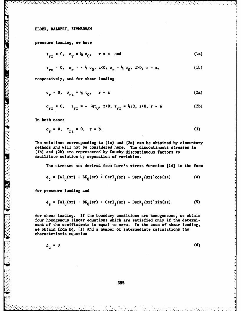
AELDER, WALBERT, ZINNER.W
pressure loading, we have
trz = O, ar = 1 ,0 r a and (la)
Trz = O, ar = - o O Z<O; or = O , z>O, r =a, (ib)
respectively, and for shear loading
r 0, a frz TOP r = a (2a)
" rz 0, Trz = k -r z<O; Trz = k'O, z>O, r = a (2b)
In both cases
a =0, =r 0, r =b. (3). r rz
The solutions corresponding to (la) and (2a) can be obtained by elementarymethods and will not be considered here. The discontinuous stresses in(lb) and (2b) are represented by Cauchy discontinuous factors tofacilitate solution by separation of variables.
The stresses are derived from Love's stress function [14] in the form
#c [A 0 (sr) + BKo(sr) + Csrll (sr) + DsrKl(sr)]cos(sz) (4)
for pressure loading and
#s [Alo(sr) + BKo(sr) + Csrll(sr) + DsrKl(sr)]sin(sz) (5)
for shear loading. If the boundary conditions are homogeneous, we obtainfour homogenous linear equations which are satisfied only if the determi-nant of the coefficients is equal to zero. In the case of shear loading,we obtain from Eq. (1) and a number of intermediate calculations thecharacteristic equation
A =0 (6)
355
-.-,.-...-......... . . ... . .•.
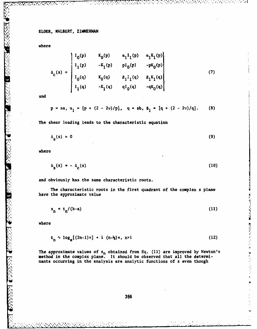
ELDER, WALBERT, ZIM4ERMAN
where
I Io(P) Ko(P) l1 1 (p) %Ixl(p)
-. I (P) - I (p) PIo(p) -pKo(P)
A (S) (7)c 1 0 (q) KO(q) 0111 (q) 1Kl(q)
I (q) "K (q) qo (q) -qK (q)
and
p = sa, l = (p + (2 - 2v)/p], q = sb, I [q 4 (2 - 2v)/q]. (8)
The shear loading leads to the characteristic equation
a (s) = (9)
where
A s(S) = - A C(S) (10)
and obviously has the same characteristic roots.
The characteristic roots in the first quadrant of the complex s plane
have the approximate value
s t/(b-a) (11)
where
tn U loge [(2n-l) ] + i (n- )w, n>l (12)
The approximate values of sn obtained from Eq. (11) are improved by Newton'smethod in the complex plane. It should be observed that all the determi-nants occurring in the analysis are analytic functions of s even though
36
.
F&~,. ~ - . . . . . . - *. . .
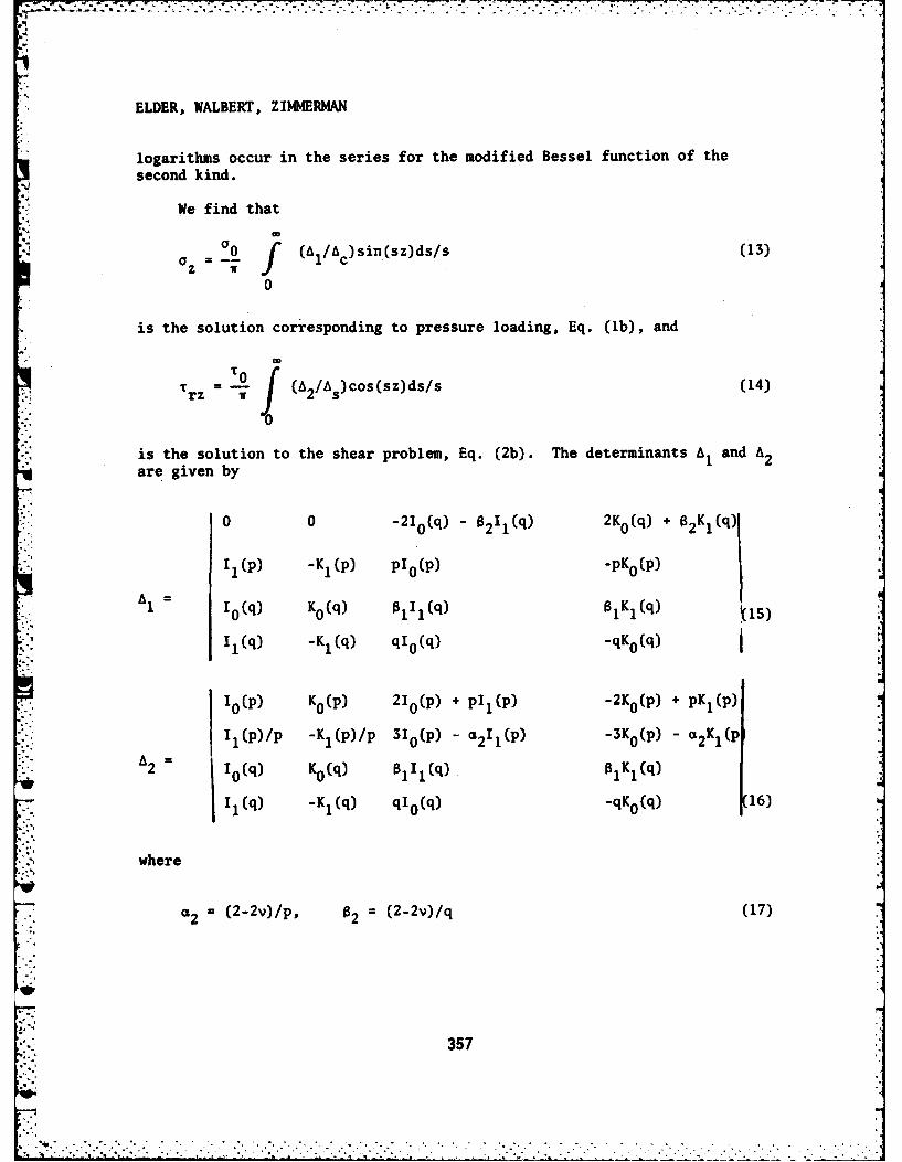
ELDER, WALBERT, ZIMMERMAN
logarithms occur in the series for the modified Bessel function of thesecond kind.
We find that
a a 0 (AI/Ac) sinC(sz)ds/s (13)az f
0
is the solution corresponding to pressure loading, Eq. (lb), and
Trz =o (A2/As)cos(sz)ds/s (14)
is the solution to the shear problem, Eq. (2b). The determinants A1 and A2are given by
0 0 -210 (q) - 8211 (q) 2Ko(q) + 82Kl(q)
I 1 (P) -K 1 (P) PI o(P) "PKo (P) i
A1I o(q) Ko(q) lIl(q) 1Kl(q) 5
11 (q) -K1 (q) qlo(q) -qK0 (q)
Io(P) Ko(p) 210 (p) + PIt(p) -2Ko(p) + pK1 (p)
II(p)/p -KI(p)/p 31o(P) - 2Ii(p) -3Ko(p) - c 2 Kl(p
2 10 (q) K0 (q) 0111 (q) 01 Kl (q)
I1 (q) -K1 (q) qlo(q) -qK (q) 16)
where
a= (2-2v)/p, 12 = (2-2v)/q (17)
357
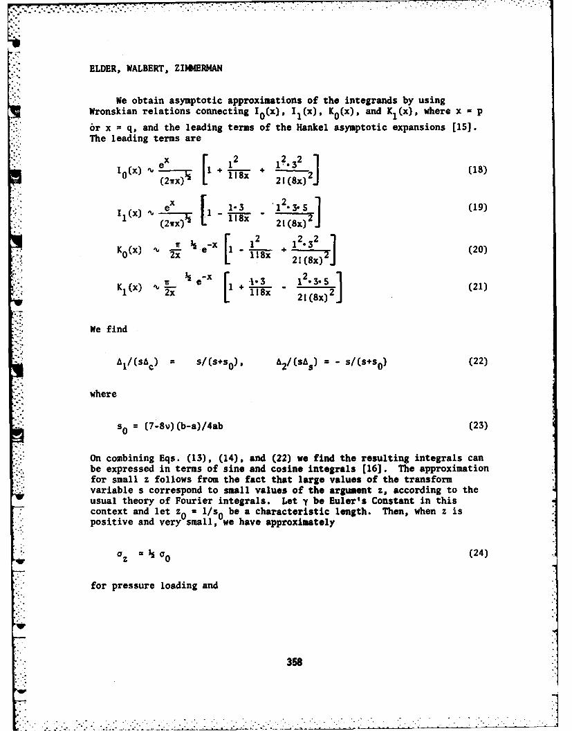
ELDER, WALBERT, ZIMI4ERMAN
We obtain asymptotic approximations of the integrands by usingWronskian relations connecting 1(x), 11(x), K0 (x), and Kl(x), where x = p
or x = q, and the leading terms of the Hankel asymptotic expansions [1S].The leading terms arex 2
( x 12 12.3 10 (2wx)I 118X 21(8x)Je 12. 3
I,() e1-3 1 i35 (19)
I1x) 18x 21(8x)2]
I (e x 12 12.3 2
K(x) e' - + j~x (21)
1K (x,
We find
A IA = s/(SSo) A2/(sA s) = ss+s O) (22)
where
s = (7-8v)(b-a)/4ab (23)
On combining Eqs. (13), (14), and (22) we find the resulting integrals canbe expressed in terms of sine and cosine integrals [16]. The approximationfor small z follows from the fact that large values of the transformvariable s correspond to small values of the argument z, according to theusual theory of Fourier integrals. Let y be Euler's Constant in thiscontext and let z = 1/sO be a characteristic length. Then, when z ispositive and very small, we have approximately
Oz 0 (24)
for pressure loading and
.8'
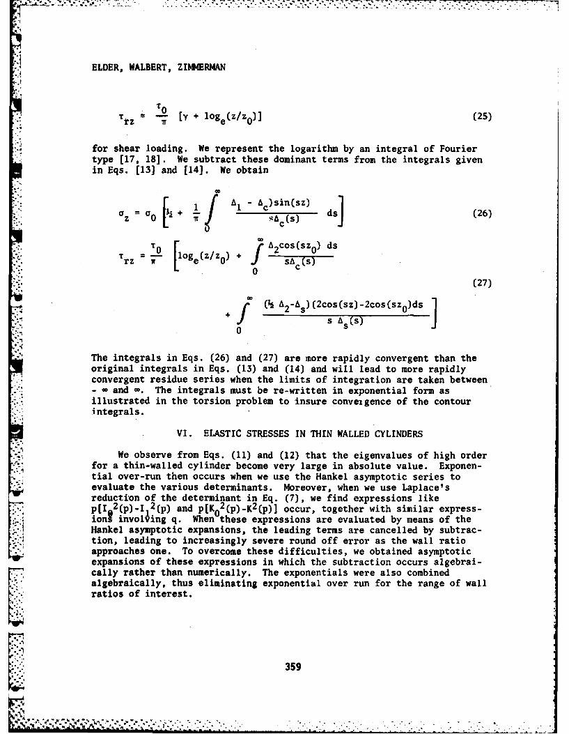
!7
ELDER, WALBERT, ZIMh4ERMAN
To [Y + loge(z/z0)] (25)
for shear loading. We represent the logarithm by an integral of Fouriertype [17, 18]. We subtract these dominant terms from the integrals givenin Eqs. [13] and [14]. We obtain
"- = 1 A1 - Ac)sin(sz) 1z= °S + A(s) ds (26)
T0 I fA 2COS(SZ0 ) dsTrz. = oge (z/z 0 ) +.s
0(27)
A2-AS)(2cos(sz)-2cos(szo)ds 1+ f s A (s)
0
The integrals in Eqs. (26) and (27) are more rapidly convergent than theoriginal integrals in Eqs. (13) and (14) and will lead to more rapidlyconvergent residue series when the limits of integration are taken between- and -. The integrals must be re-written in exponential form asillustrated in the torsion problem to insure conveigence of the contourintegrals.
VI. ELASTIC STRESSES IN THIN WALLED CYLINDERS
We observe from Eqs. (11) and (12) that the eigenvalues of high orderfor a thin-walled cylinder become very large in absolute value. Exponen-tial over-run then occurs when we use the Hankel asymptotic series toevaluate the various determinants. Moreover, when we use Laplace'sreduction of the determinant in Eq. (7), we find expressions likep[lB2 (p)-I 2 (p) and p[K0
2 (p)-K 2 (p)] occur, together with similar express-iong invol~ing q. When these expressions are evaluated by means of theHankel asymptotic expansions, the leading terms are cancelled by subtrac-tion, leading to increasingly severe round off error as the wall ratioapproaches one. To overcome these difficulties, we obtained asymptoticexpansions of these expressions in which the subtraction occurs algebrai-cally rather than numerically. The exponentials were also combinedalgebraically, thus eliminating exponential over run for the range of wallratios of interest.
~359
L .- ", ,, ,"""N, . -,- • -.r 2,

ELDER, WALBERT, ZIMMSERMAN
Let [19]
w AwI+ Bw 2 + Cw3 (28)
where
* irf[p1 02 (p)-p1 2 (p)J (29)
* w2 = [pI 0(p)K 0(p).p11 (p)Kl(p)] (30)
,= [pK0 2 (p)-pK 2 (M~,(31)
Then w satisfies the following differential equation.
p 3w' '+ 2p wi (4p 2+p)w' + w0 (32)
We find
w E an p ,n (33)2 0
where the odd numbered coefficients are zero, a0 1, a2 8 ~ and
an ( - Sn2 + 7 n- 3 )/( 4 nan2 (34)-- 2
for n>2 and even.
3 3 2 +(p3 p2 -) 82_p W1 ' + (6p + 2p )w1' +8p'8p-w'+(p 2p+l) w1 0 (35)
with a similar equation for w3 We find
360
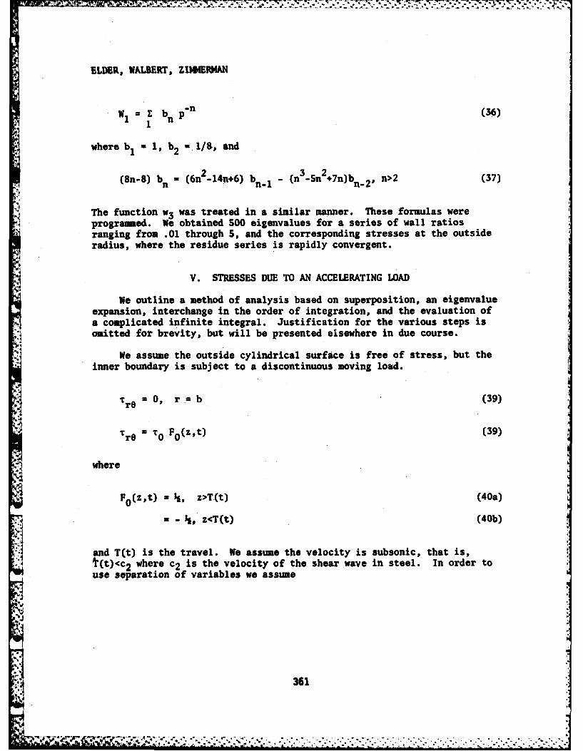
ELDER, WALBERT, ZImERmAN
Z b n P-n (36)
where b 1 , b2 - 1/8, and
(8n-8) bn - (6n2-14n+6) b n. - (n -Sn 2+7n)bn.2, n>2 (37)
The function w3 was treated in a similar manner. These formulas were: programmed. We obtained 500 eigenvalues for a series of wall ratios
ranging from .01 through 5, and the corresponding stresses at the outsideradius, where the residue series is rapidly convergent.
V. STRESSES DUE TO AN ACCELERATING LOAD
We outline a method of analysis based on superposition, an eigenvalueexpansion, interchange in the order of integration, and the evaluation ofa complicated infinite integral. Justification for the various steps isomitted for brevity, but will be presented elsewhere in due course.
We assume the outside cylindrical surface is free of stress, but theinner boundary is subject to a discontinuous moving load.
Tr = 0, r = b (39)
TrO M T0 F0(z't) (39)
where
Fo(z,t) I t, z>T(t) (40a)
- , z<T(t) (40b)
and T(t) is the travel. We assume the velocity is subsonic, that is,t(t)<c2 where c2 is the velocity of the shear wave in steel. In order touse separation of variables we assume
361
&.. . . . . . . . . . .. . . . . . . . . . . . . . . . . . . . . . . . . ...

* ELDER, WALBERT, ZIMM4ERMAN
, sin[sO(z,t)]dsFO (Z.t) 1 (41)
0
where
O(z,t) = z - T(t) (42)
We assume a solution of the form
Tr= F0(z,t) [110(r) - Z QnR(qn9 r)] +E nR(%,r)Fzt (43)1e 1 ~l
where
Rr [a2b4 4 2 4_4]R0(r)[ b- ]( (b -)](44)
and
R(%nr) =A(n) [I (%r)K 2(qnb) -K 2(%r)Y2(%b)] (45)
The eigenfunction expansion
RD (r) =E Qn R(%,r) (46)1
can be obtained either by the theory of residues or the theory oforthogonal functions. We have used both methods to determine the Fouriercoefficients Qn and the results agree. The qn are eigenvalues obtainedfrom the characteristic equation R(q,a) a 01 and are purely imaginary sincethe problem is formulated in terms of modified Bessel functions.
We assume
362
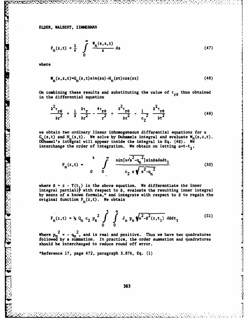
• , -. k -, : ,- - -- ' .- i j" rr - --. -- e*- -~ . - ,.- -• •. . -. - - -• - •
ELDER, WALBERT, ZIMMERMAN
I C Wn(s'z't)F n(Z't ) W f- s ds (47)
0
where
Wn(sz,t)--Gn (st)sin(sz)-Hn (st)cos(sz) (48)
On combining these results and substituting the value of Tre thus obtainedin the differential equation
a 2TrO 1 3Tr 4r 2r 1 a2Tre
2 + 3 r2 r - - ;2 (49)33r r c t
we obtain two ordinary linear inhomogeneous differential equations for aG (s,t) and H (s,t). We solve by Duhamels integral and evaluate Wn(S,Z,t).Dhamel's integral will appear inside the integral in Eq. (48). Weinterchange the order of integration. We obtain on letting a=t-t1 ,
t 2 2
F n(Z't) t sin [vs- n 2]sinosdsdt, (SO)
2 n~o- 0 c 2 s1 s2%
where 0 = z - T(t ) in the above equation. We differentiate the innerintegral partialli with respect to B, evaluate the resulting inner integralby means of a known formula,* and integrate with respect to B to regain theoriginal function F (z,t). We obtain
n
• ",t a
Fn(zt) = Qn c2 Pn2 J I 2Pddt I (51)
0 0
2 2Where p - qn , and is real and positive. Thus we have two quadraturesfollowed by a summation. In practice, the order summation and quadraturesshould be interchanged to reduce round off error.
*Reference 17, page 472, paragraph 3.876, Eq. (1)
363
.. ,
ELDER, WALBERT, ZIMMERMAN
We can readily obtain the response to a step function, then a squarewave by superposition and translation. An additional convolution willaccount for variable torque, which must be obtained from the dynamics ofthe shell.
VI. DISCUSSION AND CONCLUSIONS
We have suggested methods of improving the accuracy of calculationsbased on classical analysis without using multiple precision calculations,and which are thus suitable for a group in engineering or applied mechanics.We have obtained formulas for stationary loads, loads moving with constantvelocity, and, in the case of torsion, loads moving with arbitraryacceleration. The method presented here for solving the accelerationproblem has not been found in the literature and therefore requires carefuljustification. Additional analysis and considerable programming arerequired to obtain codes for calculating the stresses and strains. Onlythen will the results be useful in interpreting strains obtained withinstrumented gun tubes. The work is continuing with the time and resourcesavailable.
ACKNOWLEDGMENTS
The assistance of Dr. Rurik K. Loder, Ballistic Research Laboratory (BRL),in interpreting Eq. (52) is acknowledged.
J.N. WALBERTLabo:PRESENT ASSIGNMENT: Research Mathematician, Ballistic Research
". Laboratory.
PAST EXPERIENCE: Mathematician, Material Test Directorate, AberdeenProving Ground.
DEGREES HELD: BS University of Delaware, 1970; Master of Science,University of Delaware, 1972; PH.D, University of Delaware, 1975.
K.L. ZIMMERMANPRESENT ASSIGNMENT: Mathematician, Ballistic Research Laboratory.PAST EXPERIENCE: Teacher, Baltimore County, 1965-1966.
DEGREES HELD: BS, Towson State University, 1965.
364
" " , '' " '" ' " " " "' "" "" '' " " " "' ' . . . " . ." " ' " ' " , . . , _ . . ' : ' 2

• _- . V .l.. * '-
54 ELDER, WALBERT, ZIMM4ERMAN
REFERENCES
1. R. Beeuwkes, Jr., "Stresses in Thick-Walled Cylinders", WatertownArsenal Laboratory Report 730/419, Watertown Arsenal Laboratory,October 1946. Presented at the Sixth International Congress forApplied Mechanics, Paris, France, September 1946.
2. P.P. Radowski, J. I. Bluhm, 0. L. Bowie, Editors, Thick-Walled CylinderHandbook, WAL Report 893/172, December 1954. See bibliography foradditional references.
3. J. Dougall, An Analytical Theory of the Equilibrium of an IsotropicElastic Rod of Circular Cross Section, Transactions of the RoyalSociety of Edinburg, Vol. XLIX, Part IV, (No. 17), pages 895-978).(1913).
4. V. K. Prokopov, "Equilibrium of an Elastic Axisymmetrically LoadedThick-Walled Cylinder," Priladnaya mathematika i mehanika, Vol. XIII,1949 pages 135-144. Institute of Mechanics of the Academy of Sciences,USSR, FTIO Translation No. J-2589, Aberdeen Proving Ground, Maryland,Translation dated 22 August 1967.
5. A.S. Elder, K. L. Zimmerman, "Stress in a Hollow Cylinder produced bya Step Function of Pressure or Shear", Army Research Office Report75-1.
6. A.S. Elder, "Formulas for Calculating Bessel Functions of IntegralOrder and Complex Argument," BRL Report No. 1423, 1968.
7. K.L. Zimmerman, A.S. Elder, A. Depue, "User's Manual for the BRLSubroutine to Calculate Bessel Functions and Integral Order andComplex Argument", BRL Report No. TR-02068, May 1978.
8. A.S. Elder, "Stresses in a Hollow Elastic Cylinder produced by a Step., Function of Pressure or Shear," presented at the 16th Polish Solid
Mechanics Conference, Krynica, Poland, 26 August - 3 September 1974.
9. A.S. Elder and K.L. Zimmerman, Stresses in a Gun Tube produced byInternal Pressure and Shear, BRL Memorandum Report No. 2495, June,1975.
10. G.I. Taylor, Strains in a Gun Barrel Near the Driving Band of a MovingProjectile, Report AC-1851, Advisory Council on Scientific Researchand Technical Development, 19 March 1942.
365
.: .. . . . . . .; . , . . . .... - - .- ; . .

ELDER, WALBERT, ZIMMERMAN
11. H. Bucholtz, "The Confluent Hypergeometric Function", translated byH. Lichtblau and K. Wetzel, Springer-Verlag, New York Inc. 1969. SeeEq. (lOa) page 89 for required infinite integral.
12. E.T . Copson, "An Introduction to the Theory of Functions of a ComplexVariable", Oxford University Press, London, 1935. See Ex. 2, page 121,for discussion of zeros of a sequence and its limit function.
13. A.S. Elder, K.L. Zimmerman, J.N. Walbert, "Special Functions forCalculating Elastic Stresses in a Hollow Cylinder," Special BRL Reportto be published.
14. S. Timoshenko and J.N. Goodier, "Theory of Elasticity", second edition,McGraw-Hill Book Company, New York, 1951.
15. British Association for the Advancement of Science, MathematicalTables, Vol. VI, Part I, Bessel Functions of Order Zero and Unity.
16. M. Abramowitz and S.S. Stegun, Editors, Handbook of MathematicalFunctions, National Bureau of Standards, Applied Mathematics SeriesNo. 55, June, 1964.
17. I.S. Gradshteyn and I.M. Ryzhik, Tables of Integral, Series, andProducts, Fourth Edition, Academic Press, New York, 1980.
18. A.S. Elder, K.L. Zimmerman, E.M. Wineholt, "Ascending and AsymptoticSeries for Squares, Products, and Cross-Products of Modified BesselFunctions, Technical Report ARBRL-TR-02391, Ballistic ResearchLaboratory, February 1982.
366 -!
ESSENWANGER
TURBULENCE ANALYSIS BY USE OF THEFAST FOURIER TRANSFORM (U)
OSKAR M. ESSENWANGER, Ph.D.US ARMY MISSILE COMMAND
US ARMY MISSILE LABORATORY, RESEARCH DIRECTORATEREDSTONE ARSENAL, ALABAMA 35898
1. INTRODUCTION
Standard techniques in the analysis of turbulence include constructingthe spectrum of turbulence. In the last three decades most authors haveproduced the spectrum via the calculation of the autocorrelation function,Tukey (1) or Blackman and Tukey .(2). This method disclosed(among otherthings)a distinct economy in electronic data processing compared with thedetermination of the coefficients of the Fourier series. In fact, theFourier transform of the autocorrelation function is the power spectraldensity, or in short, the spectrum, e.g., Tennekes and Lumley (3), p. 214.
Later Cooley and Tukey (4) introduced the Fast Fourier Transform (FFT)by which spectral values are calculated from the amplitudes of the Fourierseries with even less computer time than is used by the autocorrelationmethod. Thus, "canned" programs of the FFT can be found readily on modernelectronic data processing systems while the "old-fashioned" technique viathe autocorrelation function is fading away. Some investigators maytacitly accept the postulation that the results from the FFT provide avalid spectrum in the analysis of turbulence. This postulation is examinedin the following study.
- . It.will be demonstrated that the FFT can be utilized for turbulenceanalysis but with certain reservations. The main problem is the calcula-
., tion of the slope of the spectrum for a longer data series and the scatterof the standardized squared amplitudes for the FFT. The latter may produceoutliers which could bias the slope of the spectral density.
It will also be shown that readings of the Gill anemometer (u-v-w).at one-second time intervals produced features in agreement with turbulencetheory.
W
367
".? I
ESS MANGER
Finally, the FFT implies that the turbulence fluctuations can besuperimposed upon the "stationary" profile for simulation studies of Armymissile systems.
2. TURBULENCE AND POWER SPECTRUM
The presence of turbulence requires that the energy E(x) in thepower spectral density of the one-dimensional velocity (e.g., the wind'su-component) decreases as a function of the (standardized) wave number k:
E(k) ac kcsA [1]
This decrease follows the Kolmogorov-Obukhov-Corrsin hypothesis onisotropic turbulence in the inertial subrange; see Tennekes and Lumley (3),p. 266, Priestly (5), p. 61, Hinze (6), p. 194, etc. The Kolmogorovconstant a and the dissipation C (here a constant) are of secondaryinterest. The reader is referred to the quoted literature for more details
. on a and e.
The relationship to the power spectral density L is:
k2L A2 (k) dk- E(k) [2]
Ici
where the wave number k - J/p and p is the basic period. Computation ofthe power spectral density via the autocorrelation function was introducedby Tukey (1), see also Blackman and Tukey (2) or Panofsky and Brier (7).Power spectrum and Fourier series are associated by:
L = iA 2/2cY2 3th 2
the squared standardized amplitude of the j th Fourier term; a2 is thevariance.
In double logarithmic coordinates:
in(L) = const - (5/3)in k - const - bin k [4]
This is a linear equation with slope b - -5/3. Thus, turbulence isdifferent from white noise, a random process, whose spectral characteristic
In L - const [S]
with fluctuations of Lj produced by random errors.
368
ESSENWANGER
18
12
14
12
0
0 5 10 15 20 25 30 35 40 46 s0 55 so
WAVE NUM50R K
Fig. 1. Power spectrum of the windehear component Au, 1-second recordings,60 Aecond4. 2 1'U level 2 at 9.1 mn, level 1 at 5.5 in, maximum lag
2.O ~ MORINCH LMU. SLOPI -IM3
at-
OAM
am:
WeOM L CUD"
corints Naiu lag 300 sconds. ue
369
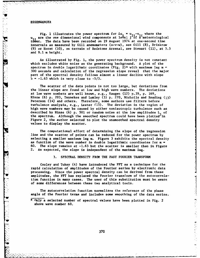
ESSENWANGER
Fig. 1 illustrates the power spectrum for Au = u21.-u i where thej of a meteorological
tier. The data have been recorded on 19 August 1974 at one-second timeintervals as measured by Gill anemometers (u-v-w), see Gill (8), Drinkrow(9) or Horst (10), on terrain of Redstone Arsenal, see Stewart (11), at 5.5and 9.1 m height.
As illustrated by Fig. 1, the power spectrum density is not constantwhich excludes white noise as the generating background. A plot of thespectrum in double logarithmic coordinates (Fig. 2)* with maximum lag m300 seconds and calculation of the regression slope reveal that the majorpart of the spectral density follows almost a linear decline with slopeb = -1.63 which is very close to -5/3.
The scatter of the data points is not too large, but deviations fromthe linear slope are found at low and high wave numbers. The deviationsat low wave numbers are well known, e.g., Haugen (12) p.39, p. 169,Hinze (6) p. 203, Tennekes and Lumley (3) p. 270, Nicholls and Reading (13)Peterson (14) and others. Therefore, some authors use filters before
"turbulence analysis, e.g., Lester (15). The deviation in the region ofhigh wave numbers may be caused by either nonisotropic turbulence such asdescribed by Hinze (6) p. 501 or random noise at the low amplitudes L ofthe spectrum. Although the smoothed spectrum could have been plotted inFigure 2, the author selected to plot the unsmoothed spectral densityvalues to display the scatter.
The computational effort of determining the slope of the regressionline and the scatter of points can be reduced for the power spectrum byselecting a smaller maximum lag m. Figure 3 exhibits the spectral densityas function of the wave number in double logarithmic coordinates for m =60. The slope remains at -1.63 but the scatter is smaller than in Figure2. As expected, the slope is independent of the maximum lag.
3. SPECTRAL DENSITY FROM THE FAST FOURIER TRANSFORM
Cooley and Tukey (4) have introduced the FFT as a technique for therapid calculation of amplitudes of the Fourier series by electronic dataprocessing. Since the power spectral density can be derived from theseamplitudes, the FFT has replaced the Fourier transform of the autocorrela-tion function in many cases. The user of this substitution must be awareof some differences between these two analytical tools.
The autocorrelation function normalizes the reference of the phase
angle of the Fourier terms and includes some smoothing of the data series.
• Only a selected number of spectral values have been plotted in Fig. 2above wave number 60.
3
-i 370
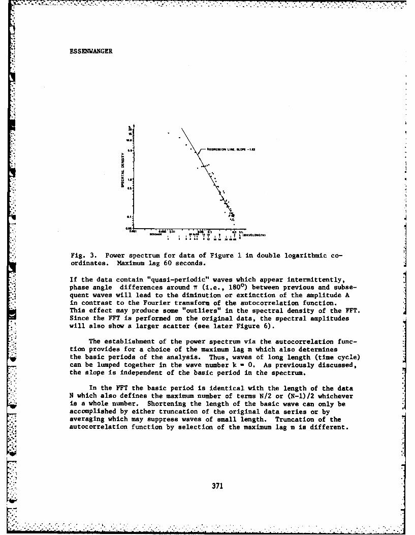
.1 ESSENWANGER
20
IA
$. REGRIEMION LINE. ILOPE -1.3
Molin 3f I fI I L W VLIGs
ordinates. Maximum lag 60 seconds.
.... If the data contain ",quasi-periodic" waves which appear intermittently,;-,. phase angle differences around w (i.e., 180 ) between previous and subse-
,.' quent waves will lead to the diminution or extinction of the amplitude A
,-."in contrast to the Fourier transform of the autocorrelation function.This effect may produce some "outliers" in the spectral density of the FFT.
• Since the FFT is performed n the original data, the spectral amplitudes
:, will also show a larger scatter (see later Figure 6).
,...
- :,The establishment of the power spectrum via the autocorrelation func-"-,;tion provides for a choice of the maximum lag m which also determines~the basic periods of the analysis. Thus, waves of long length (time cycle)
can be lumped together in the wave number k - 0. As previously discussed,
,.the slope is independent of the basic period in the spectrum.
.0o1
i" ' o r' 'In the FFT the basic period is identical with the length of the data
r:.' N which also defines the maximum number of terms N/2 or (N-1)/2 whicheveris a whole number. Shortening the length of the basic wave can only beaccomplshed by either truncation of the original data series or byaveraging which may suppress waves of small length. Truncation of the
autocorrelation function by selection of the maximum lag m is different.
I 371
can be ... lupe togethe in th wav numbe k . A.rviul.isusd,,,'-thesloe isindeendnt o th basic.. .period. .. .i. the.. set.._ , . ...- .
In the FF.T. the basic. period.._,-,. is ''- ; idnialwt th legt of the data. ,.....'.
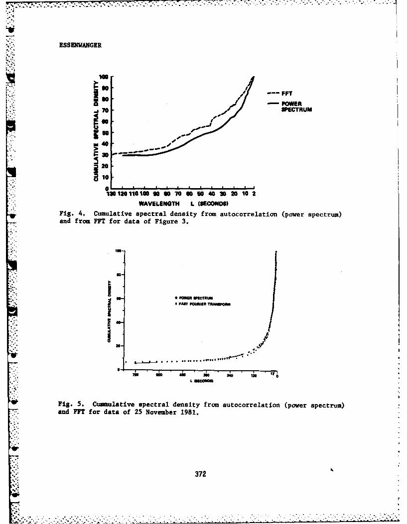
ESSENWANGER
POWER7 7 SPECTRUM
40
20S10
130 120 110 100 90 90 70 60 60 40 30 20 10 2WAVELENGTH L (SECONDS)
Fig. 4. Cumulative spectral density from autocorrelation (power spectrum)and from FFT for data of Figure 3.
A
Fig. 5. Cumnulative spectral density from autocorrelation (power spectrum)and FIT for data of 25 November 1981.
372

ESSENWANGER
Consequently, it is no surprise that the cummulative spectral densityobtained from the Fourier transform of the autocorrelation function and theFFT for the data of Fig. 2 or 3 exhibit some difference (Fig. 4). A
" disparity is not always found.
Fig. 5 exhibits the cumulative power spectral density of the Fouriertransform spectrum and of the FFT for data recorded on 25 November 1981 atthe AFGL Weather Test Facility at Otis AFB, Cape Cod, Massachusetts,measured with a Climatronic Wind Mark I System. As illustrated in thiscase, the result from the Fourier transform deviates only minimally fromthe one obtained by the FFT. Although the wave numbers (1-60) in bothgraphs (Fig. 4 and 5) are the same, the wave length (time cycle) is differ-ent because the data have been taken at 6-second intervals. In short,some spectra produced by the two tools may differ and others do not.
Fig. 6 provides the individual (squared and standardized) amplitudescalculated by the FFT for the same data as Fig. 2 and 3. The slope of theregression line b -1.63 which is identical with the result from the
I=
Ii: a"i * ~ 'di'n aw-e--t a
M -
Fig. 6. Spectral density from FFT in double logarithmic coordinates,19 August 1974 data.
373
r:
ESSENWANGER
power spectrum but b was not easily obtained. Spectral valuesof wave numbers with k over 400 and below 10 were truncatedwhich isequivalent to the application of a bandpass filter.
The weakness of the FFT is the disproportionate weight which high wavenumbers have in the ordinary process of calculation of a regression line byleast square methods and determination of its slope b. As outlined, thephase angle effect may produce some outliers which also could distort thevalue of the slope. Two methods are recommended to minimize the effect ofdisproportionate weight and outliers: truncation or median value regres-
sion.
Usually the truncation points (band pass filter) are not known apriori. Thus, they cannot be affixed for electronic data processingbefore computation of the regression line is made. An iterative trunca-tion process is recommended starting with omitting one or two waves atlow wave numbers (k = 1,2) and a multiple of waves with high numbers (e.g.,for N/2 - 512, omit k-494 through 512). Then the residual variance andthe slope are computed. The residual variance is:
.:)2 v- (Y-l I/N [6]
where Y is the analytical value of InL from the regression liae and Yiis XnL The slope b will stabilize after some iterative steps; v willdecrease.
The iterative process can be combined with a statistical evaluationof the slope b from iterative processes j by checking b against bor checking vRJ against v l. Test methods have been d~scribed byJ
+ 1
Anscombe (16) or Anscombe and Tukey (17).
The fitting of a regression line by ordinary least square methodsmay not eliminate the biasing effect of outriers,although after somestabilization of bj and VR ,excessive deviations JY.-y. I could be omittedand the slo e b recalculatdd. Although a threshold z could be determinedand values ]I -Yil>lz could be excluded,the procedure may be elaborate.A simple but robust method was suggested by Lawson (18) based on the -
median.
Lawson recommends the division of data into three sections, determin-ing the median of yj for the extreme sections, and then calculating theregression line from the two median values. This process is simple butmay produce an uncertain statistical error. Therefore, for the FFT, thisauthor suggests more than three sections depending on the data length N.An equal number of data in these individual sections is not required.
374
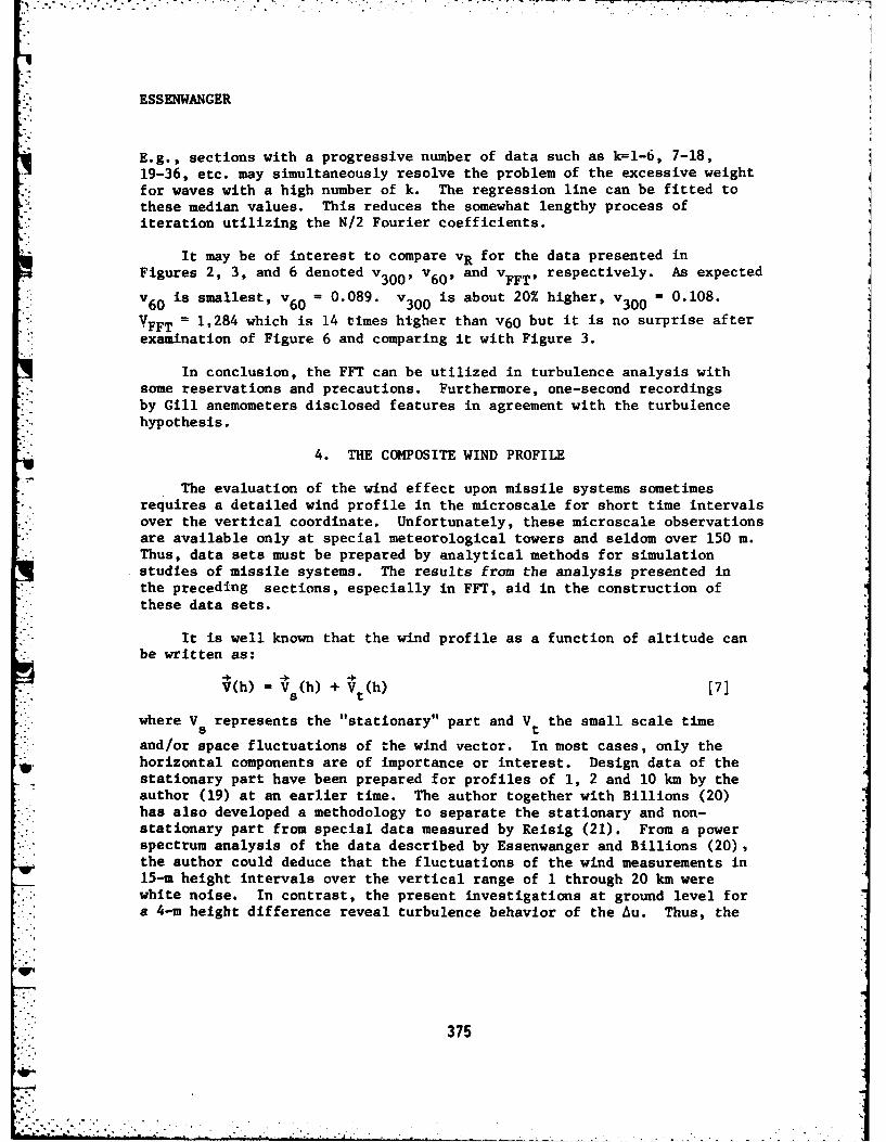
ESSENWANGER
E.g., sections with a progressive number of data such as k=l-6, 7-18,19-36, etc. may simultaneously resolve the problem of the excessive weightfor waves with a high number of k. The regression line can be fitted tothese median values. This reduces the somewhat lengthy process ofiteration utilizing the N/2 Fourier coefficients.
It may be of interest to compare vR for the data presented in
Figures 2, 3, and 6 denoted v3 0 0, v6 0, and vFFT, respectively. As expected
is smallest, v 0.089. v is about 20% higher, v300 = 0.108., : 60 ssmletv60 v30030
. VFFT 1,284 which is 14 times higher than v60 but it is no surprise afterexamination of Figure 6 and comparing it with Figure 3.
In conclusion, the FFT can be utilized in turbulence analysis withsome reservations and precautions. Furthermore, one-second recordingsby Gill anemometers disclosed features in agreement with the turbulencehypothesis.
4. THE COMPOSITE WIND PROFILE
The evaluation of the wind effect upon missile systems sometimesrequires a detailed wind profile in the microscale for short time intervalsover the vertical coordinate. Unfortunately, these microscale observationsare available only at special meteorological towers and seldom over 150 m.Thus, data sets must be prepared by analytical methods for simulationstudies of missile systems. The results from the analysis presented inthe preceding sections, especially in FFT, aid in the construction ofthese data sets.
It is well known that the wind profile as a function of altitude canbe written as:
V (h) = s(h) + Vt(h) [7]
where V represents the "stationary" part and V the small scale time5 t
and/or space fluctuations of the wind vector. In most cases, only theVhorizontal components are of importance or interest. Design data of the
stationary part have been prepared for profiles of 1, 2 and 10 km by theauthor (19) at an earlier time. The author together with Billions (20)has also developed a methodology to separate the stationary and non-stationary part from special data measured by Reisig (21). From a powerspectrum analysis of the data described by Essenwanger and Billions (20),the author could deduce that the fluctuations of the wind measurements in15-m height intervals over the vertical range of 1 through 20 km werewhite noise. In contrast, the present investigations at ground level fora 4-m height difference reveal turbulence behavior of the Au. Thus, the
375

ESSENWANGER
author postulates from the tentative results that differences of the wind
component in the lowest 1 or 2 km may follow turbulence structure ratherthan white noise, transforming to the latter above that range except inregions with known turbulence such as clear air turbulence. The study
continues for confirmation of this postulation. We may now compose theu component for the wind from:
u(h) u Us(h) + Au (h) [8]
where u (h) denotes the stationary part and:k2
Au(h) - Z A +) [9]
J=kl
Here -hj j2w h/H where h is the altitude (h = 1,..., H).
In [9] the amplitudes A follow the slope b = -5/3, i.e.,
2 tn(Ak) - B-(5/3) Lnk [10]
B is a constant to be explained below. The phase angles 0 are randomlydistributed, i.e., 0 has a rectangular distribution. Theiwaves k < kmay be considered as part of the stationary profile u (h). The upperboundary is k < N/2 or k2 < (N-l)/2.
An equivalent formula is valid for the horizontal (rectangular)v(h) component of the wind.
Formulae [9] and [10] were utilized to simulate the fluctuations ofAu as a function of height (Figure 7). These fluctuations can be super-imposed upon u (h). This set of data should prove to be better suitedfor the evaluation of the small scale wind effect than the presenttechnique of assuming a 95% wind profile and superimposing a 95% gust.
The investigations will continue with determination of numericalvalues for B. Theoretically an initial value can be found for k = 1.Then B - Xn(A2 ),but it should be noticed that Ai is not necessarily
*identical with the first Fourier term of the FFT as we learn fromFigures 2, 3, and 6.
5. TIME AVERAGES AND DIFFERENCES OF WINDSPEED (MICRO-SCALE)
. Common windspeed measurements (such as by ordinary cup anemometers)may be considered as time averages because of either a slow instrumentalresponse time or a built-in time integration. In fact, this averaging isintended for conventional measurements to report a "representative" wind-speed in synoptic observations. These measurements display a "meso-scale"
376
* -. . * - - - . .
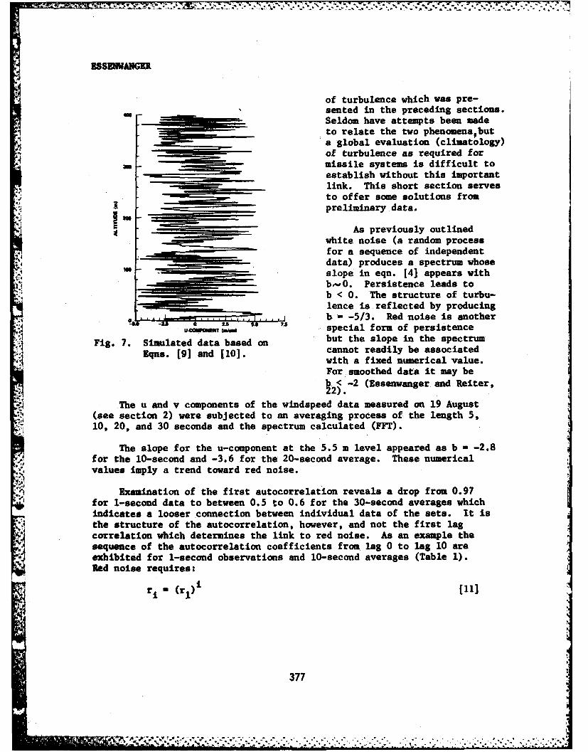
ZSSEWANGER
of turbulence which was pre-sented in the preceding sections.Seldom have attempts been madeto relate the two phenomenabut
4a global evaluation (climatology)of turbulence as required formissile systems is difficult toestablish without this importantlink. This short section servesto offer some solutions frompreliminary data.
As previously outlinedwhite noise (a random processfor a sequence of independentdata) produces a spectrum whoseslope in eqn. [4] appears withbO. Persistence leads tob < 0. The structure of turbu-lence is reflected by producingb - -5/3. Red noise is another
MPo .5 5.0 t special form of persistence
Fig. 7. Simulated data based on but the slope in the spectrum
Eqns. [9] and [10]. cannot readily be associatedwith a fixed numerical value.For smoothed data it may be
b < -2 (Essenwanger and Reiter,
22).
The u and v components of the windspeed data measured on 19 August(see section 2) were subjected to an averaging process of the length 5,10, 20, and 30 seconds and the spectrum calculated (FFT).
The slope for the u-component at the 5.5 m level appeared as b - -2.8for the 10-second and -3.6 for the 20-second average. These numericalvalues imply a trend toward red noise.
Examination of the first autocorrelation reveals a drop from 0.97for 1-second data to between 0.5 to 0.6 for the 30-second averages whichindicates a looser connection between individual data of the sets. It isthe structure of the autocorrelation, however, and not the first lagcorrelation which determines the link to red noise. As an example thesequence of the autocorrelation coefficients from lag 0 to lag 10 areexhibited for 1-second observations and 10-second averages (Table 1).Red noise requires:
- (r1)i [11
377
', I, ..
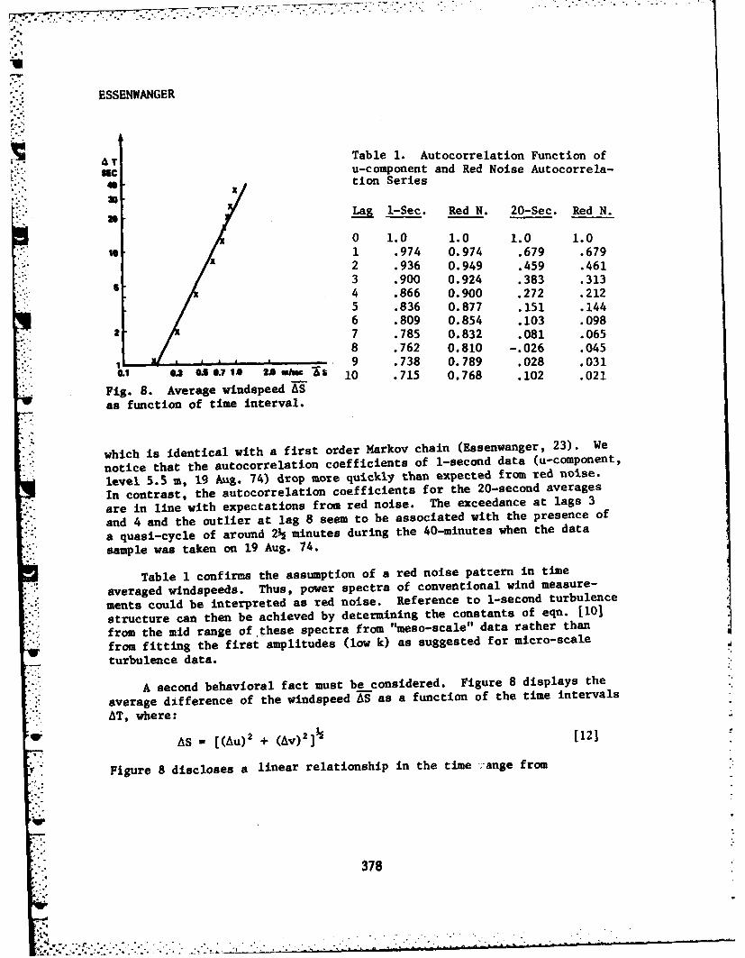
ESSENWANGER
AT Table 1. Autocorrelation Function of
u-component and Red Noise Autocorrela-a x tion Series
S1-Sec. Red N. 20-Sec. Red N.
0 1.0 1.0 1.0 1.0
"9 1 .974 0.974 .679 .6792 .936 0.949 .459 .461
3 .900 0.924 .383 .313
5 4 .866 0.900 .272 .2125 .836 0.877 .151 .1446 .809 0.854 .103 .098
7 .785 0.832 .081 .0658 .762 0.810 -.026 .045
01 . 0. 9 .738 0.789 .028 .031.e AS 10 .715 0.768 .102 .021
Fig. 8. Average windspeed AS
as function of time interval.
which is identical with a first order Markov chain (Essenwanger, 23). We
notice that the autocorrelation coefficients of 1-second data (u-component,
level 5.5 m, 19 Aug. 74) drop more quickly than expected from red noise.
In contrast, the autocorrelation coefficients for the 20-second averages
are in line with expectations from red noise. The exceedance at lags 3
and 4 and the outlier at lag 8 seem to be associated with the presence of
a quasi-cycle of around 2 minutes during the 40-minutes when the data
sample was taken on 19 Aug. 74.
Table 1 confirms the assumption of a red noise pattern in time
averaged windspeeds. Thus, power spectra of conventional wind measure-
ments could be interpreted as red noise. Reference to 1-second turbulence
structure can then be achieved by determining the constants of eqn. [101
from the mid range of these spectra from "meso-scale" data rather than
from fitting the first amplitudes (low k) as suggested for micro-scale
turbulence data.
A second behavioral fact must be considered. Figure 8 displays the
average difference of the windspeed AS as a function of the time intervals
AT, where:
AS = [(Au)2 + (AV)2[; 112]
V Figure 8 discloses a linear relationship in the time ;ange from
378
ESSENWANGER
1 to 40 seconds differences with a slope of 0.5. Since the first 30seconds were of primary interest here, the continuation of the data afterthe 40-second time interval is not shown, but it stabilizes at a constantvalue for longer time intervals. This result in micro-scale resemblesearlier work by Neumann (24) who has demonstrated with customary wind dataat the "meso-scale" for readings half an hour apart that the relativevariability tends to a constant value as the time interval increases.
If the time structure as disclosed by Fig. 8 is not automatically metduring the derivation of analytical data by eqn. [10],it may be necessaryto find a solution to include the time structure on a vertical scale. Thisinvestigation is continuing.
The results for the 19 Aug 74 data sample were not completely con-clusive, and further studies on data samples such as the 25 Nov 81 datawill continue. However, one tentative result can be deduced. The numeri-cal value of the slope in Figure 8 is 0.5. This is the same numericalvalue as derived for the windshear relationship for small intervals(Essenwanger and Reiter, 22,and Essenwanger, 25). Essenwanger and Reiter j(22) could interpret the slope of 0.5 as a mixture between smoothed dataand turbulence fluctuations. If this interpretation can be applied to thedata of Fig. 8, a separation of the "stationary and'non-stationary" partsuch as required in eqn. [7] is already the solution, and the time intervalrelation would implicitly appea. ]
S 6. CONCLUSION i
The author has shown that the Fast Fourier Transform is a usefultool in turbulence analysis and the lack of "canned" programs of theFourier transform of the autocorrelation function poses no serious problem.The user is cautioned, however, to be aware of the differences between thespectra produced by these two techniques.
A data sample procured with the Gill anemometer recorded at one-second time intervals reflect agreement with the turbulence hypothesis(Fig. 2,3).
The FFT has the advantage that turbulence data can be readilyexpressed as a Fourier series. The amplitude relationship is expressedby eqns. [4] and (10] while the phase angles are randomly distributed.Although a set of phase angles can be constructed from random generatorsin electronic data processing, a simple technique would be a substitutionfrom a set of empirical turbulence data.
The author has given an example of an analytically produced "non-stationary" set of data which could be superimposed on the "stationary"wind profile. These inferred data sets can be established where special
379
ESSENWANGER
tower measurements are not available such as for altitudes beyond tower
measurements and/or for geographic locations without tower measurements.These composed sets of wind data are better suited than present techniquesfor the assessment of the turbulence Impact upon effectiveness, instru-mental or missile sensitivity, and field use of systems such as DAFFR,
Assault Breaker, CSWS, etc. by combining the "stationary" and "non-
stationary" effect into one data set.
ACKNOWLEDGMENT
The author expresses his appreciation to Dr. Dorathy A. Stewart for
her critical comments and the editorial review of the manuscript. Mrs.
Alexa M. Mims deserves most of the credit for the preparation of the
computer programs. My thanks go to Mr. Larry J. Levitt for his assistance
in the preparation of the figures. The simulated data (Fig. 7) were pre-
pared by Dr. Shi Tsan Wu. Finally, Mrs. Louise H. Cooksey deserves the
credit for her patience and expeditious typing of the manuscript, and to
CPT James C. Weyman, Air Force Geoph. Lab., for the special data of Fig.5.
REFERENCES
1. Tukey, J. W., 1949. The Sampling Theory of Power Spectrum Estimates.; NAVEXOS-P-735, Woods Hole. Office of Naval Research, p. 47-67.
2. Blackman, R. B. and J. W. Tukey, 1958. The Measurement of PowerSpectra. Dover Publ. Inc., New York, pp 190.
3. Tennekes, H., and J. L. Lumley, 1973. A First Course in Turbulence.MIT Press, Cambridge, Mass. pp 300.
4. Cooley and J. W. Tukey, 1965. An Algorithm for the Machine Calcula-tion of Complex Fourier Series. Math. Comput. Vol. 19, p. 297-301.
5. Priestley, C. H. B.,1959. Turbulent Transfer in the Lower Atmosphere.University of Chicago Press, Chicago, pp 130.
6. Hinze, J. 0., 1959. Turbulence, An Introduction to its Mechanism andTheory, McGraw Hill. New York, pp 586.
7. Panofsky, H. A. and G. W.Brier, 1958. Some Applications of Statisticsto Meteorology. Pennsyl.vania State University, pp 224.
8. Gill, G.' C., 1975. Development and Use of the Gill UVW AnemometerBoundary-Layer Meteorol., Vol. 8, p. 475-495.
9. Drinkrow, R., 1972. A Solution to the Paired Gill Anemometer ResponseFunction. J. Appl. Meteorol., Vol. 11, p. 76-80.
380
ESSENWANGER
10. Horst, T. W., 1973. Corrections for Response Errors in a Three-Component Propeller Anemometer. J. Appl. Meteorol., Vol. 12, p.
716-725.
11. Stewart, D. A., 1975. Turbulence Measurements from the Army Gas
Dynamic Laser Range. US Army Missile Command Report RR-75-8, pp 25.
12. Haugen, D. A., 1973, editor. Workshop on Micrometeorology. Am.
Meteor. Soc., Boston, pp 392.
13. Nicholls, S. and C. J. Readings, 1981. Spectral Characteristics ofSurface Layer Turbulence Over the Sea. Qu. J. Roy. Meteorol. Soc.Vol. 107, p. 591-614.
14. Peterson, E. L., 1976. A Model for the Simulation of AtmosphericTurbulence. J. Appl. Meteorol. Vol. 15, p. 571-587.
15. Lester, P., 1972. An Fnergy Budget for Intermittent Turbulence inthe Free Atmosphere. J. Appl. Meteorol., Vol. 11, p. 90-98.
16. Anscombe, F. J., 1967. Topics in the Investigation of LinearRelations Fittee by the Method of Least Squares. J. Roy. Stat.
Soc., B, Vol. 29, p. 1-52.
17. Anscombe, F. J. and J. W. Tukey, 1963. The Examination and Analysisof Residuals. TechnometricsVol. 5, p. 141-160.
18. Lawson, J. S., 1982. Application of Robust Regression in Designed
Industrial Experiments. J. Qual. Techn., Vol. 14, p. 19-33.
19. Essenwanger, 0. M., 1973. Wind Profile Parameters in the Ground Layerand Troposph. at Mid Latitudes. US Army Missile Comm.RR-73-6, pp 27.
20. Essenwanger, 0. M. and N. S. Billions, 1965. The Stationary and Non-Stationary Wind Profile. Pure and Appl. Geoph. Vol. 60, p. 160-166.
21. Reisig, G. H. R., 1956. Instantaneous and Continuous Wind Measure-ments up to the Higher Stratosphere. J. Meteorol. Vol. 13,p 448-455.
22. Essenwanger, 0. M., and E. R. Reiter, 1969. Power Spectrum, StructureFunction, Vertical Wind Shear, and Turbulence in Troposph. and
Stratosph. Arch. Meteorol. Geoph. Bioklim, A, Vol. 18, p. 17-24.
*W 23. Essenwanger, 0. M., 1980. On Red Noise and Quasi-Periodicity in the
Time Series of Atmospheric Temperature. Statistical Climatology,p. 165-181. Editors: S. Ikeda, E. Suzuki, E. Uchida and M. M.Yoshino. Elsevier, Amsterdam, pp 388.
24. Neumann, J. 1967. Wind Variability for Time Intervals of MediumLength. J. Appl. Meteor., Vol. 6, p. 587-589.
25. Essenwanger, 0. M., 1963. On the Derivation of Frequ. Distrib. ofVector Shear Values for Small Shear Intervals. Geofis. Pura Appl.Vol 56, p. 216-224.
381
AD-R128 811 PROCEEDINGS OF THE 1982 ARMY SCIENCE CONFERENCE HELD AT 5/6THE UNITED STRTES..(U) DEPUTY CHIEF OF STAFF FORRESEARCH DEVELOPMENT AND RCQUISITIO.. 18 JUN 82
UNCLASSIFIED F/G 5/2 NL
EEIIIE.EIIIIllllEllEllllhEEBhEEBhhhhhhhEEhlhhlhlhhhhhImhhhhhhlhhhhEESlfljlllf IIllffEhhhlhhhhhEEEI
lz -W2 7 *
Lw -5 | 1.0 = Im &M
ILIlik L ' " 1 WL I
MICROCOPY NUSOUTIO TEST CHART
MICROCOPY RESOWTIO01 TEST CHART mr& u ol anowme2-mN-ANATIOA BUEA OF SrANOAIIOS-1913-A
MICROCOI RE~ou~nIoN TEICROCOPY RESOLUUTION TEST, CHART -
I"JL
E.....E /J .uI
I W
t .
.12 11.25
MICROCOPY OUTt TEST CRYRT.. ... ... " i .. .PU AU_ OF STAM -1 3-A ... --
"1 -0
to.a Wo" Ili m. woa
I
. .. /= 'i , -o .L2 116. .4
Figucia, Williams, Kirkwood, Koza
MECHANISM OF IMPROVED BALLISTIC FABRIC PERFORMOCE (U)
F. FICJCIA *C. WILLIAMSBe KIHKIO0DW. KOZA
U.S. ARM! NATICK RESEAR. AND DWMJOPMNT LABORATORIESNATICK, MASSACHUSh1IT
Protection of U.S. infantry personnel in ground warfare environmentsrequires constant technical vigilance on the part of Government scientiststo assure that the most advanced state-of-the art is being implemented forthe benefit of the soldier. This paper addresses that requirement asrelated to protection of personnel against fragmenting munitions.
Though the level of ballistic protection already achieved and cur-rently being fielded exceeds anything ever developed in the past, thepotential exists for even greater improvement in protection against frag-menting threats, and the need exists for protection against new threats.New developments in weapons technology utilizing surface coatings, novelshape factors and higher density materials continually challenge the levelof protection achievable with existing armor systems.
A more intensified scientific approach must be devoted to the ballis-tic problem to provide adequate protection against the rapidly changingthreat patterns in the field. The problem is a difficult one for a numberof reasons. Fibrous materials have proven their worth both ballisticallyand functionally, but relatively little scientific information has beendeveloped in this area as compared to other material disciplines. Pene-
*i. tration mechanics of such materials are physically unique and somewhatconfounding, and are not clearly defined. Finally, scientific contribu-tions from the private sector have been essentially non-existent due tothe marginal cmoaicial attraction of armor items.
It is expected that through this paper a firmer scientific basewill be established and that the future use of this technology will even-tually lead to a better understanding of the physical interaction betweenflexible fabric and penetrating projectile.
383
.,, ..r ,-',.- s..,...:,...- - ..,-. .... -...... ...... *.. ...... ... .. . .. . - -. ... .- .
, Figucia, Williams, Kirkwood, Koza
G NERtAL APPROACH
The approach taken in this study is to analyze the projectileimpact of a fabric in logical steps, and perform laboratory experimentsto quantify the various physical responses which are active. The eventinvolves a number of fiber characteristics and penetration mechanismsinteracting in microseconds of time.
The process begins with the initial contact of a projectile upon anorthogonally woven fabric. This sets up a potential exchange of projec-tile kinetic energy into yarn tensile stress-strain energy. As long asthe tensile mode of response remains in effect, the energy of the projec-tile is translated longitudinally along the yarns in continuous pulseswhich can be thought of as wavelets of stress-strain energy. These travelat velocities which vary with the crystalline character of the targetmaterial. The amount of yarn which becomes involved through this mech-anism increases from the time of initial contact until the projectilepenetrates the fabric and the strain is released.
- At the same time as the in-plane exchange of energy takes place,projectile energy is also dissipated through fabric transverse motion.The forward thrust of the projectile carries target fabric out of itsoriginal planes The displaced material takes the shape of a pyramid (1,2)whose base and height dimensions continually increase until penetrationoccurs*.
The problem is approached through an analysis of the energy dissipa-tion in these two modes (planar and transverse). Theoretical energyabsorption is derived after quantification of appropriate parameters. Thecomputation for planar energy encompasses penetration time, wave velocity,number of contacted yarns, and yarn energy absorption potentLal. Compu-tation of the transverse component of energy involves the shape and dimen-
sions of the fabric distortion, the average missile/fabric velocity, andthe mass of the fabric displaced.
These computed energy absorptions are then compared with that meas-ured in actual tests. The agreement obtained will establish the importanceof the studied parameters and their application to future efforts in thefield.
MATMALSThe main thrust of this analysis was toward the behavior of woven
fabrics as opposed to other constructional forms.Fabrics representative of two polymer types were studied; nylon 66
(polyamide) and Kevlar 29 (polyaramid). Fabrics were selected with con-structional features as nearly identical as possible. Characteristics ofthe two materials are tabulated below.
384
.. . . . . . . . . .
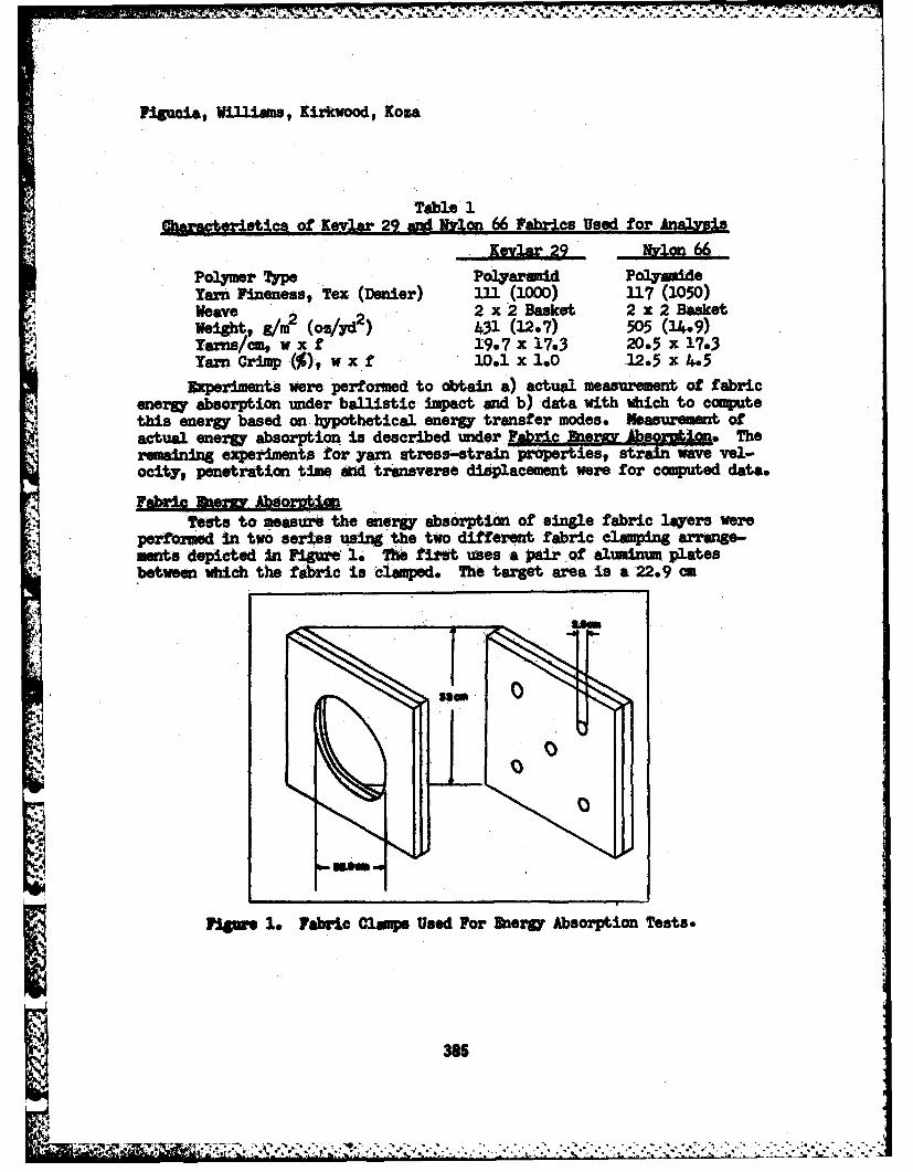
Piucia, Williams, Kirkwood, Kosa
Table 1Chaaterstics of KevIar 29 and Irlon 66 t'bdrics Used for Analysis
Kevlar 29 Nylon 66
Polymer Type Poyar d PolyideYarn Fineness, Tex (Denier) 111 (1000) 117 (1050)Weave 2 x 2 Basket 2 x 2 BasketWeSght, S/r 2 (oz/i ) 431 (12.7) 505 (14.9)Yarns/cm, w x f 19.7 x 17.3 20.5 x 17.3Yarn Crimp (),w x f 10.1 x 1.0 12.5 x 4.5
Experiments were performed to obtain a) actual measurement of fabricenergy absorption under ballistic impact and b) data with which to computethis energy based on hypothetical energy transfer modes. s t ofactual energy absorption is described under .abric herxv Absor M.o. Theremaining experiments for yarn stress-strain properties, strain wave vel-ocity, penetration time and transverse displacement were for computed data.
Tests to measure the energy absorption of single fabric layers wereperformed in two series using the two different fabric clamping arrange-.ents depictedIn Figural. The fifrstUses a pairof alumnum platesbetween which the fabric is clamped. The target area is a 22.9 cm
141
bqq
Mre le Fabric Claws Used For ne Absorption Test.
., . .. .. ... . .. ..- , , ., . , . . . .. ..,, , ....
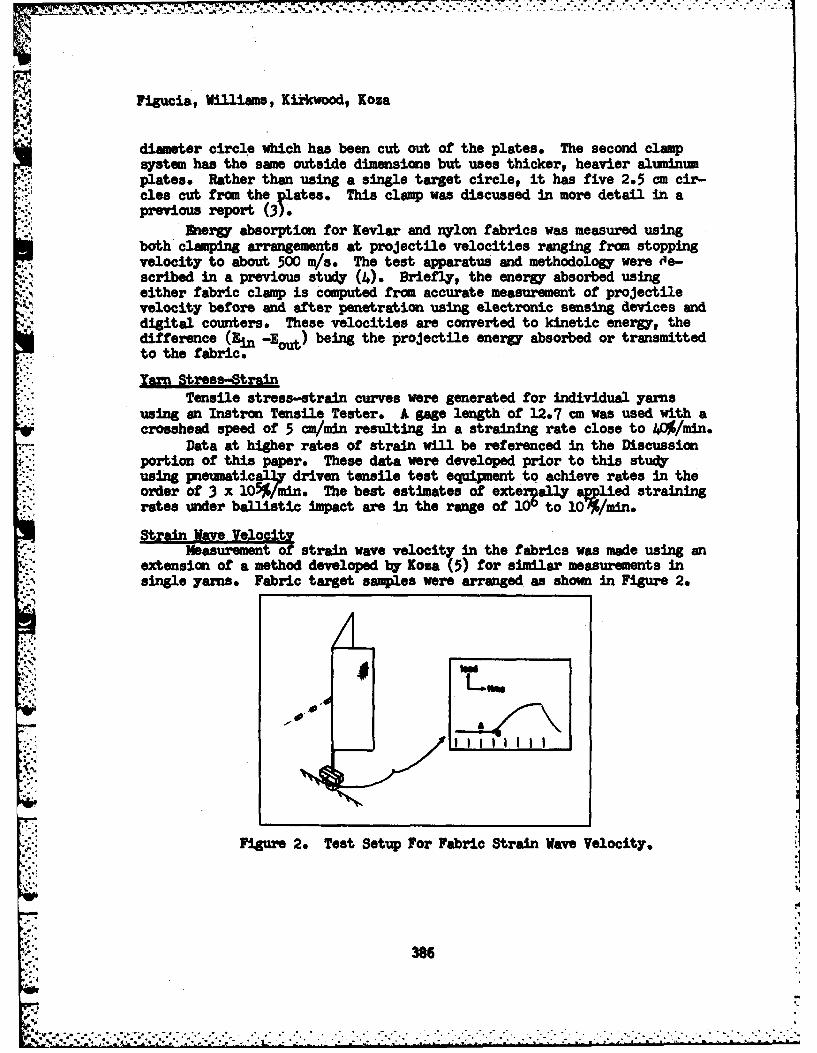
Figucia, Williams, Kfrkwood, boza
diameter circle which has been cut out of the plates. The second clampsystem has the same outside dimensions but uses thicker, heavier aluminumplates. Rather than using a single target circle, it has five 2.5 cm cir-clee cut from the slates. This clamp was discussed in more detail in aprevious report (3)
Energy absorption for Kevlar and nylon fabrics was measured usingboth clamping arrangements at projectile velocities ranging from stoppingvelocity to about 500 m/s. The test apparatus and methodology were de-scribed in a previous study (4). Briefly, the energy absorbed using
4.' either fabric clamp is computed from accurate measurement of projectilevelocity before and after penetration using electronic sensing devices and
digital counters. These velocities are converted to kinetic energy, thedifference (Bin -Eout) being the projectile energy absorbed or transmittedto the fabric.
Tarn Stress-StrainTensile stress-strain curves were generated for individual yarns
using an Instron Tensile Tester* A gage length of 12.7 cm was used with acrosshead speed of 5 c/min resulting in a straining rate close to 40%/mn.
Data at higher rates of strain will be referenced in the Discussionportion of this paper. These data were developed prior to this studyusing pneumatical7 driven tensile test equipment to achieve rates in theorder of 3 x 10⁵ /min. The best estimates of extergally a ad strainingrates under ballistic impact are in the range of 10 to 10O/min.
Strain Wave VelocityMeasurement of strain wave velocity in the fabrics was made using an
extension of a method developed by Kosa (5) for similar measurements insingle yams. Fabric target samples were arranged as shown in Figure 2.
,::,iFigure 2e Test Setup For Fabric Strain Wave Velocity.
- '; 386
LLN

Figucia, Williams, Kirkwood, Koza
The fabric was clamped at the top but only 10 yarns extending from thebottom edge were clamped below. These were the ends of the same yarns tobe contacted by the projectile at the center of the fabric. A piezoelec-tric crystal load cell was fastened to the bottom clamp as shown and itsoutput directed to an oscilloscope. Knowing the distance between the loadcell and the point of contact of the projectile with the fabric, it wasonly necessary to measure the time of travel of the wave over this dis-tance to obtain wave velocity. To accomplish this the test was performedwith the room in darkness and with a multiflash generator and camera setup to photograph the flight of the projectile. The first flash was syn-chronized with the sweep of the dual oscilloscope beams. The upper beamrecorded load cell response vertically vs time horizontally. The lowerbeam gave a spike signal for each flash. The example in Figure 2 showsthat the projectile contacted the fabric on the 3rd flash which on theload-time recording is a point of no apparent load (point A). The res-ponse of the load cell occurs at point B a measurable time later. Thedistance AB represents the travel time of the wave.
Wave velocities were measured in this way for both nylon and Kevlarfabrics in both warp and filling directions. Projectile velocities ofapproximately 305 n/s were used for these tests.
Penetration TimeThe time elapsed during penetration was measured over the same range
of projectile velocities as used for the fabric energy absorption tests.The fabric clamp with the 22.9 cm diameter hole in the center was modifiedto facilitate this experiment. A 0.6 cm slot was bored upward from thebottom edge of the clamp on the inside face of each plate. This relievedabout 10 yarns from the clamping pressure during testing. These were thesame yarns contacted by the projectile at the center of the target. Theywere extended downward to the clamp and load cell which were coupled to-gether below the target as shown in Figure 3. Penetration time (t) was
tieF 4_
Figure 3. Setup For Penetration Time Tests.
387
[r.
A _1
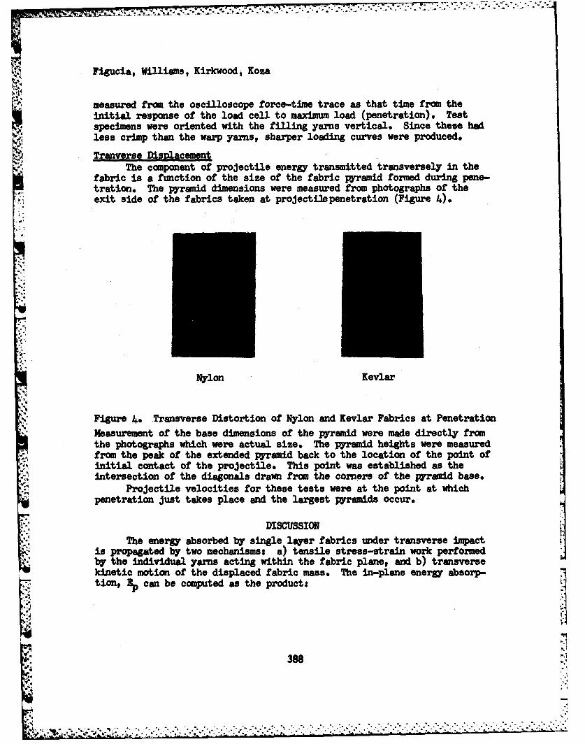
Figucia, Williams, Kirkwood, Koza
measured from the oscilloscope force-time trace as that time from theinitial response of the load cell to maximum load (penetration). Testspecimens were oriented with the filling yarns vertical. Since these hadless crimp than the warp yarns, sharper loading curves were produced.
Tranverse DisplacementThe component of projectile energy transmitted transversely in the
fabric is a function of the size of the fabric pyramid formed during pene-tration. The pyramid dimensions were measured from photographs of theexit side of the fabrics taken at projectilepenetration (Figure 4).
"4.
Nylon Kevlar
Figure 4. Transverse Distortion of Nylon and Kevlar Fabrics at Penetration
Measurement of the base dimensions of the pyramid were made directly fromthe photographs which were actual size. The pyramid heights were measuredfrom the peak of the extended pyramid back to the location of the point ofinitial contact of the projectile. This point was established as theintersection of the diagonals drawn from the corners of the pyramid base.
Projectile velocities for these tests were at the point at whichpenetration just takes place and the largest pyramids occur.
DISCUSSION
The energy absorbed by single layer fabrics under transverse impactis propagated by two mechanisms: a) tensile stress-strain work performedby the individual yarns acting within the fabric plane, and b) transversekinetic motion of the displaced fabric mass. The in-plane energy absorp-tion, % can be computed as the products
C38
4* 88 ".14
..
' V , - - : . .. -. ..., " "".'- " ""." -" . ." - -" -" " ':',: " '"'"- '.'."'. '-" ."' ,'. ""'-,".'" '",",' ,'" ' ' "' " ' '",-- " " 4-
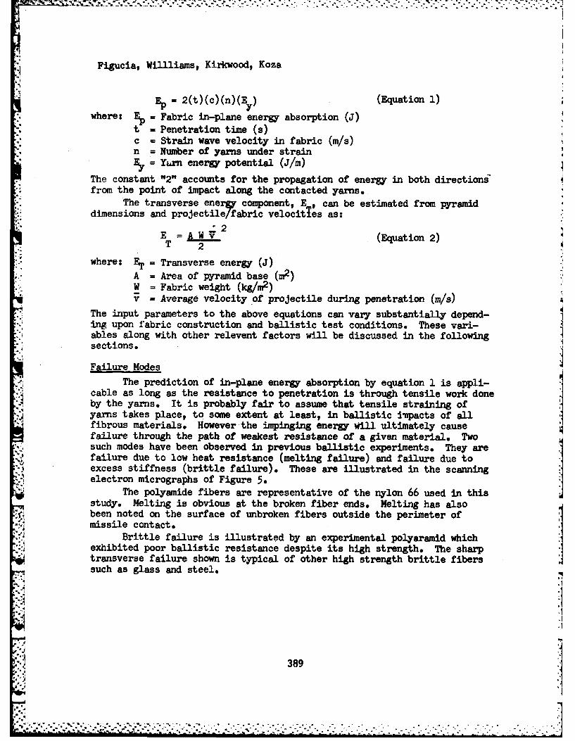
Figucia, Wililiams, Kirkwood, Koza
= 2(t)(c)(n)(E ) (Equation 1)y
where: E = Fabric in-plane energy absorption (J)
t - Penetration time (s)c = Strain wave velocity in fabric (m/s)n = Number of yarns under strain
= Yurn energy potential (J/m)
The constant "2" accounts for the propagation of energy in both directions'from the point of impact along the contacted yarns.
The transverse ener component, E , can be estimated from pyramiddimensions and projectile/fabric velocities as:
E (Equation 2)
T 2where: E = Transverse energy (J)"1
A = Area of pyramid base (m2 )W = Fabric weight (kg/n 2 )v = Average velocity of projectile during penetration (m/s)
The input parameters to the above equations can vary substantially depend-ing upon fabric construction and ballistic test conditions. These vari-ables along with other relevent factors will be discussed in the followingsections.
Failure Modes
The prediction of in-plane energy absorption by equation 1 is appli-cable as long as the resistance to penetration is through tensile work doneby the yams. It is probably fair to assume that tensile straining ofyarns takes place, to some extent at least, in ballistic impacts of allfibrous materials. However the impinging energy will ultimately causefailure through the path of weakest resistance of a given material. Twosuch modes have been observed in previous ballistic experiments. They arefailure due to low heat resistance (melting failure) and failure due toexcess stiffness (brittle failure). These are illustrated in the scanningelectron micrographs of Figure 5.
The polyamide fibers are representative of the nylon 66 used in thisstudy. Melting is obvious at the broken fiber ends. Melting has alsobeen noted on the surface of unbroken fibers outside the perimeter ofmissile contact.
Brittle failure is illustrated by an experimental polyaramid whichexhibited poor ballistic resistance despite its high strength. The sharptransverse failure shown is typical of other high strength brittle fiberssuch as glass and steel.
389
."
4" -. - ' ."-". -" " " " " " " " - " " . " - - ." "- ' - -. . .. .. . . ..- - ... .. '1
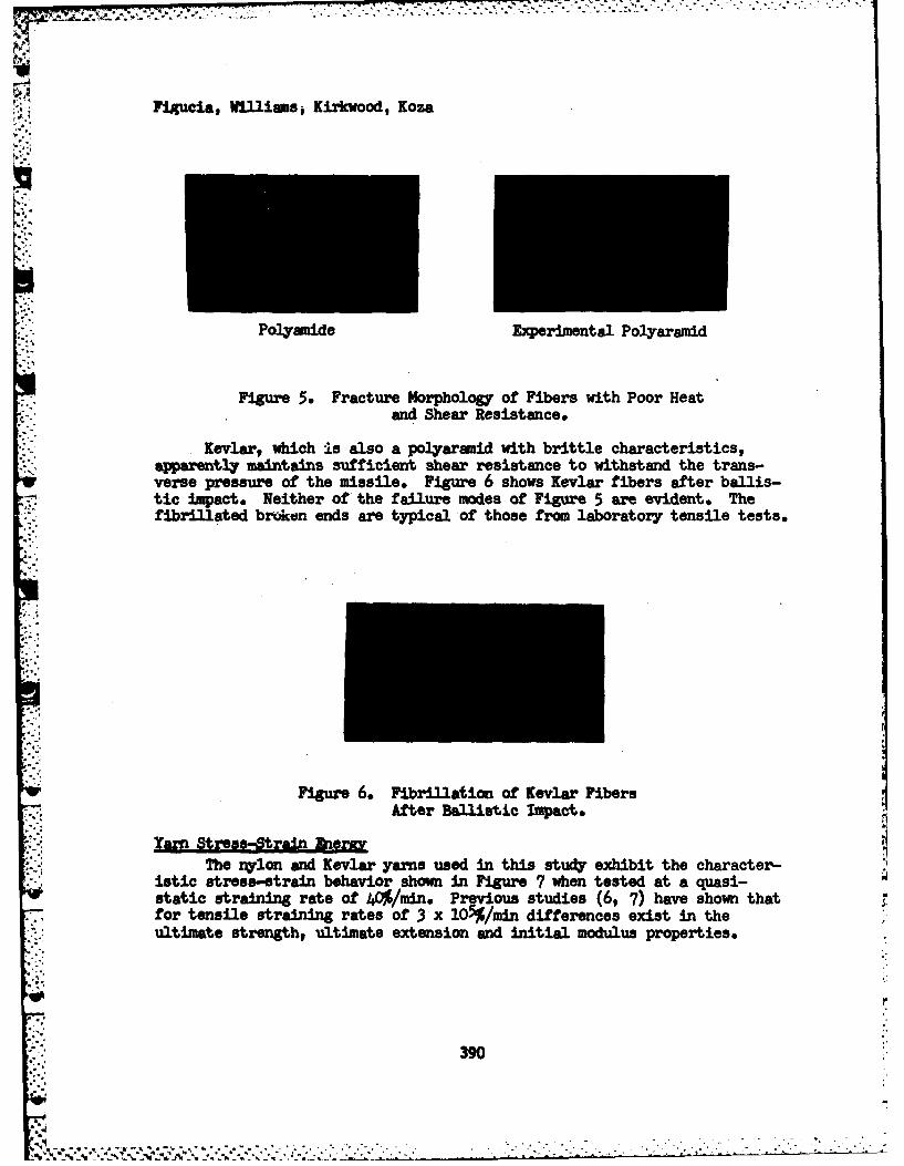
Figucia, Williamsi Kirkwood, Koza
Polyamide Experimental Polyaramid
Figure 5. Fracture orphology of Fibers with Poor Heatand Shear Resistance.
Kevlar, which is also a polyaramid with brittle characteristics,apparently maintains sufficient shear resistance to withstand the trans-verse pressure of the missile. Figure 6 shows Kevlar fibers after ballis-tic impact. Neither of the failure modes of Figure 5 are evident. Thefibrillated broken ends are typical of those from laboratory tensile tests.
Figure 6. Fibrillation of Kevlar FibersAfter Ballistic Impact*
Yarn Stress-Strain kwro-The nylon and Kevlar yarns used in this study exhibit the character-
istic stress-strain behavior shown in Figure 7 when tested at a quasi-static straining rate of 4O /min. Previous studies (6, 7) have shown thatfor tensile straining rates of 3 x lOS%/min differences exist in theultimate strength, ultimate extension and initial modulus properties.
390
---------------------------------. . . . .
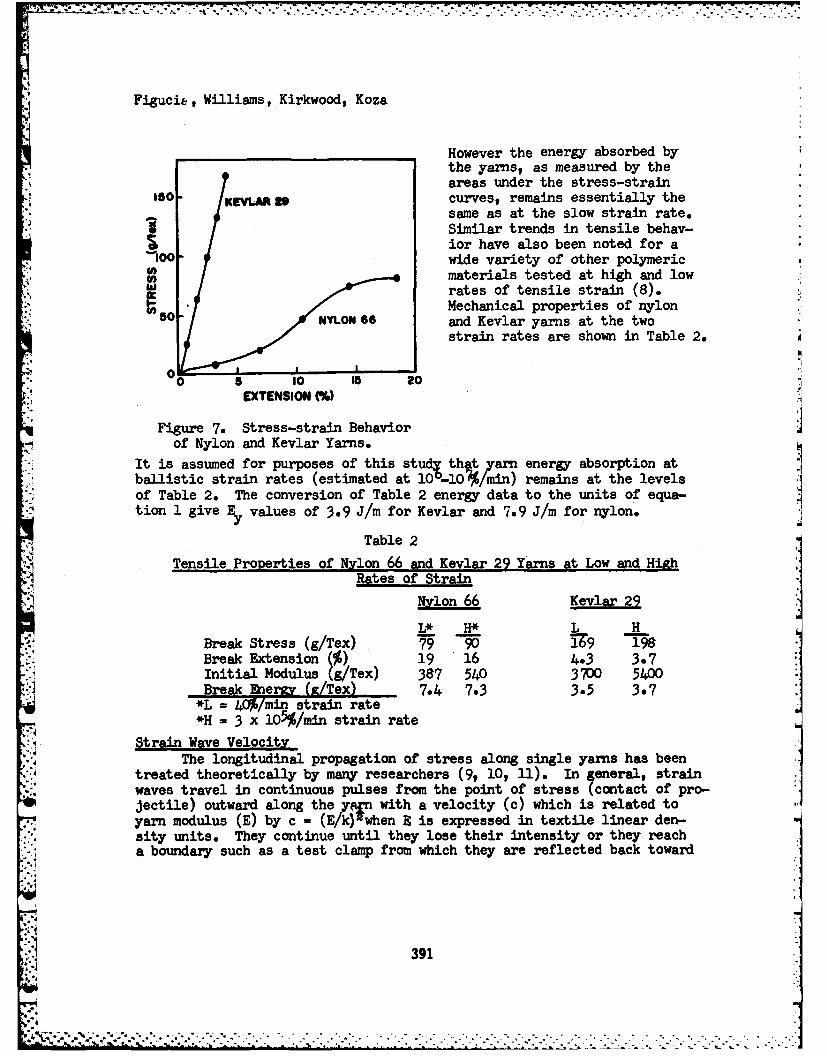
Figucia, Williams, Kirkwood, Koza
However the energy absorbed by* -the yarns, as measured by the
areas under the stress-strainISO KEVLAR 9 curves, remains essentially the
same as at the slow strain rate.SSimilar trends in tensile behav-
ior have also been noted for aS100 wide variety of other polymeric
) materials tested at high and lowrates of tensile strain (8).Mechanical properties of nylon
NYLON 66 and Kevlar yarns at the twostrain rates are shown in Table 2.
EXTENSION (%)
Figure 7. Stress-strain Behaviorof Nylon and Kevlar Yarns.
It is assumed for purposes of this study that yarn energy absorption atballistic strain rates (estimated at lO0-lO%'/min) remains at the levelsof Table 2. The conversion of Table 2 energy data to the units of equa-
ytion 1 give E values of 3.9 J/m for Kevlar and 7.9 J/m for nylon.
Table 2
Tensile Properties of Nylon 66 and Kevlar 29 Yarns at Low and HighRates of Strain
Nylon 66 Kevlar 29
L* H* L HBreak Stress (g/Tex) go9 198Break Extension (%) 19 16 4.3 3.7Initial Modulus (gTex) 387 540 3700 5400Break Enerwy (iE/Tex) 7.4 7.3 3.5 3.7*L 40/min strain rate*H = 3 x 10⁵%/min strain rate
Strain Wave VelocityThe longitudinal propagation of stress along single yarns has been
treated theoretically by many researchers (9, 10, ii). In general, strainwaves travel in continuous pulses from the point of stress (contact of pro-jectile) outward along the yem with a velocity (c) which is related toyarn modulus (E) by c = (E/k)mwhen E is expressed in textile linear den- Nsity units. They continue until they lose their intensity or they reacha boundary such as a test clamp from which they are reflected back toward
391
.% . , . , - o - .,. - , - . - . - , . . . . . . . . . .
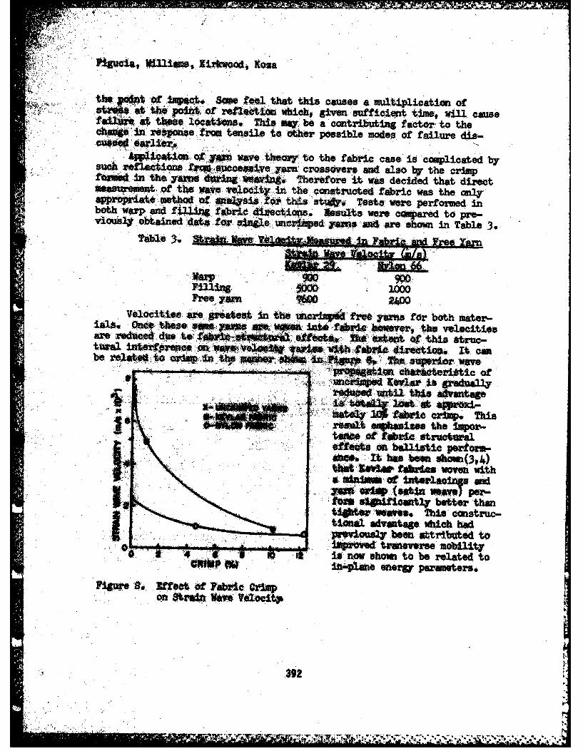
FMtaia *MUliM Rrwood, Kow.
th a~toi tmWOt. 3*O feel that this caUses a mi4tiplication Ofstre~ tt thi pcih't of reflection wich givensufficient time, wil causefailsM, at tese lo-cations.' This MWq be a contributing factor to the
cagin flsponqe trom tensile to other possible modes of failure dis-cus earlir
S w1*to W;r wave theory to the fabric case is'cauplicated byreflctin fc4 soce~yeyencrossovers wad also by the crimp
formd An the yams. during ,Wtvigo Therefore it was decided that directof the wave nelooty in the constructed fabric was the only,
approprite method of W&4B5Ji I pr this, .t*,i Tests were performed inboth wrp and figisig fabric directions. Results were 'capeared to pre-vious41j obtained data for aiil. wicrt-ped yensaend are shorn in Table 3.Table Wae3*A M%4dt
Free yan 2400Velocities are* greatest, In the mclpkfret yartis for both mater-
ialso One* these se- arp w:1- ,it fbi oeeitevlcare~ nucede tteow t*ave~e'w ate wi t hveth fbidre veloItiesbe r4atpd to or-np-in'hmneJ .tn-iup hspeirwv
Wlcbipd Kelari pra-l
Mt. tha beene ahiop.mide0 A, resut tnw O ies wohe nwith
t~tog" ofabri. Tinstruc-tia .0 adva t tck harorm
*~aMU O I s now shorn t bre atedr~ozzStrfliftV been fl Wlitt
.3 392
M ~ r -7$%'~t
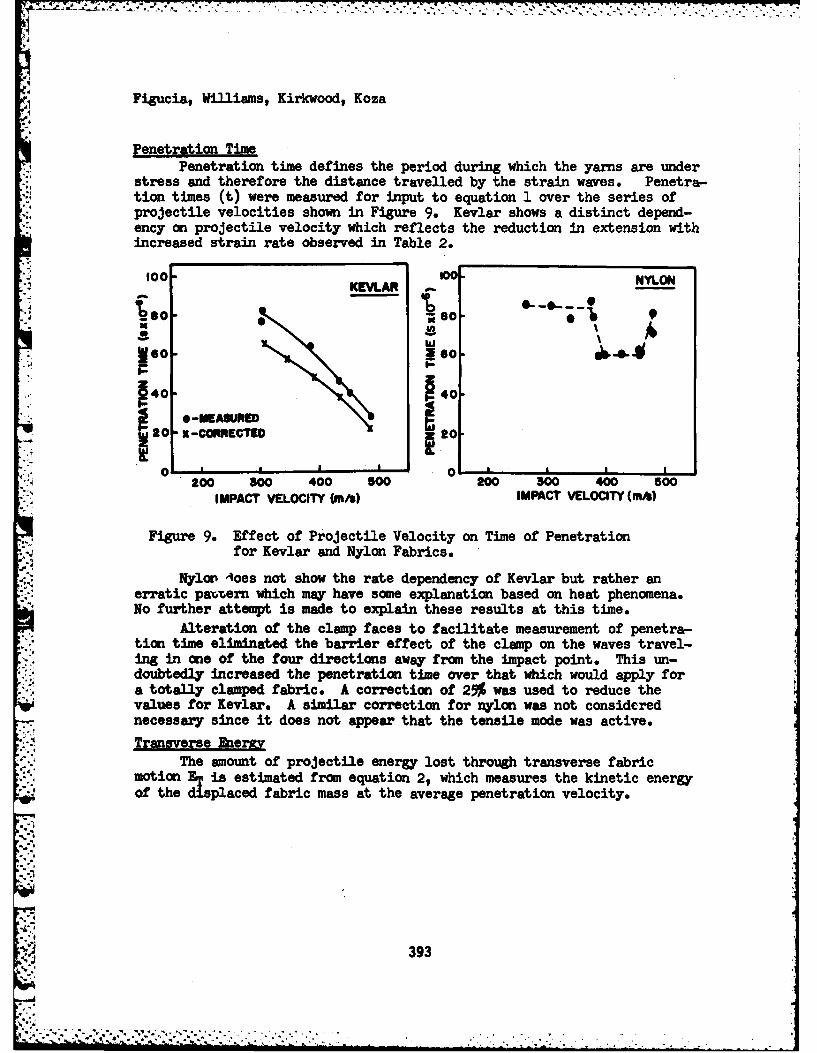
I1 Figucia, Williams, Kirkwood, Koza
Penetration TimePenetration time defines the period during which the yarns are under
stress and therefore the distance travelled by the strain waves. Penetra-tion times (t) were measured for input to equation 1 over the series ofprojectile velocities shown in Figure 9. Kevlar shows a distinct depend-ency on projectile velocity which reflects the reduction in extension withincreased strain rate observed in Table 2.
OO KEVLAR NYLON
. ~ ~ 8 -O -O
!,o ;so9*W
4- , 0°
00 0
2002 3t 400 500IMPACT VELOCITY (m/9) IMPACT VELOCITY (ms)
Figure 9. Effect of Projectile Velocity on Time of Penetrationfor Kevlar and Nylon Fabrics.
NyJor Aoes not show the rate dependency of Kevlar but rather anerratic payern which may have some explanation based on heat phenomena.No further attempt is made to explain these results at this time.
Alteration of the clamp faces to facilitate measurement of penetra-tion time eliminated the barrier effect of the clamp on the waves travel-ing in one of the four directions away from the impact point. This un-doubtedly increased the penetration time over that which would apply fora totally clamped fabric. A correction of 25% was used to reduce thevalues for Kevlar. A similar correction for nylon was not considerednecessary since it does not appear that the tensile mode was active.
Transverse EherpyThe amount of projectile energy lost through transverse fabric
motion ET is estimated from equation 2, which measures the kinetic energyof the displaced fabric mass at the average penetration velocity.
393

Figucia, Williams, Kirkwood, Koza
N." Measurements were made of the fabric pyramids formed during impact atvelocities near that at which penetration just occurs and the largestpyramids are formed. -values obtained under these conditions were usedto estimate those at hiher velocities through the use of data of Roylance(2). This resulted in a reduction of transverse energy absorption withincreasing impact velocity (Figure 10).
"I KEVLAR
4I
SOPPING
0 I I I
200 300 400 500IM ACT VELOCITY (m/)
Figure 10. Effect of Projectile Velocity on TransverseEnergy Absorption of Kevlar.
Theoretical vs. Experimental EnerEy AbsorptionSingle layer fabric samples were tested for energy absorption over
a range of projectile velocities using 2.5 and 22,9 cm diameter clamps.Figure 11 shows the effects of the clamp bomdaries on the results. Themaximum energ absorbed by the two materials at the velocity of initialpenetration (left most point) is reduced about 50% in going from thelarger to the smaller target. This difference becomes smaller howeveras projectile velocity increases due to the accompanying reduction inpenetration time and wave propagation distance. The reduction in energyabsorption (50%) is not proportional to the ratio of target diameters(11%). Considerable yarn strain was evident in all directions beyond the2.5 cm boundaries, indicating that the strain wave intensity was suffi-cient to force through the nearby boundaries resulting in more yarninvolvement and energy absorption levels greater than predicted.
*0.
394
. ,.-
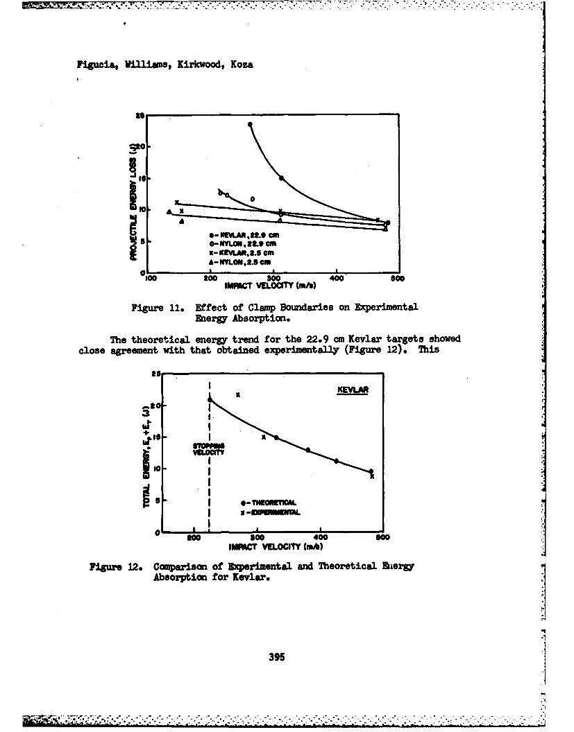
Figucia, Williams, Kirkwoodq Koza.
LX 0
*-N!VLA,223SCM
xKEVLAR, .5 cmA-NYL0U,3.S Cm
610 00 300 400 500IMPACT VELOCITY Wmio)
Figure 11, Effect of Clamp Boundaries on ExperimentalEniergy Absorption.
The theoretical energy trend for the 22.9 cm Keviar targets showedclose agreement with that obtained experimental~ly (Figure 12). This
as
+ is
VEIT TVEOIY m
10-i
*-HERT5A
-WWWAUNIIII
am. . . . . . . . . . . . . . .
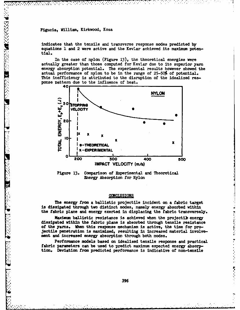
K Figucia, William, Kirkwood, Koza
indicates that the tensile and transverse response modes predicted byequations 1 and 2 were active and the Kevlar achieved its maximum poten-tial.
In the case of nylon (Figure 13), the theoretical energies wereactually greater than those computed for Kevlar due to its superior yarnenergy absorption potential. The experimental results however showed theactual performance of nylon to be in the range of 25-50% of potential.This inefficiency is attributed to the disruption of the idealized res-ponse pattern due to the influence of heat.
40
NYLON
W VELOCrIT •2 0-
hi S•
.j, I 0to- I
I X-EXPERIMENTALo I I I , I
200 300 400 500IMPACT VELOCITY (m/s)
Figure 13. Comparison of Experimental and TheoreticalEnergy Absorption for Nylon
CONCLSIONS
The energy from a ballistic projectile incident on a fabric targetis dissipated through two distinct modes, namely energy absorbed withinthe fabric plane and energy exerted in displacing the fabric transversely.
Maximum ballistic resistance is achieved when the projectib energydissipated within the fabric plane is absorbed through tensile resistanceof the yarns. When this response mechanism is active, the time for pro-jectile penetration is maximized, resulting in increased material involve-ment and increased energy absorption through both modes.
Performance models based on idealized tensile response and practicalfabric parameters can be used to predict maximum expected energy absorp-tion. Deviation from predicted performance is indicative of non-tensile
396

Figucia, Williams, Kirkwood, Koza
failure responses such as melting and shear which severely reduce ballis-tic efficiency. The scanning electron microscope is a valuable devicefor verification of such failure patterns.
Strain wave velocity is the most important parameter influencingballistic performance. Rapid propagation of stress away from the point ofimpact incorporates more material into the resistive process. It alsodistributes the energy such that the energy/mass ratio is kept belowlevels at which shear or heat failures may otherwise occur. Strain wavevelocity is significantly affected by fabric construction. Potential forimproved ballistic performance exists through loose fabric weave designand reduced yarn crimp.
(1) Hearle, U. of Manchester Inst. of Sci & Tech., 1st Periodic Report,
Contract No. DAJA37-69-C-0532.
(2) Roylance, D., and Wang, S., US Army R&D Labs, TR-4O/021 (1979).(3) Figucia, F., US Army Natick R&D Labs, TR--80/O08, (1979).(4) Figucia, F., Arny Science Conference Proceedings, Vol. II, po 29,
(5) Kosa, W., US Aruy Natick R&D Labs, IFL-249, publication pending,(1962).
(6) Figuciat F., Weiner, L., and Laible, R., Polymer Ekg & Science,Vol. II, No. 4, (1971).
(7) Unpublished data, US AruV Natick R&D Labs, Notebooks No. 5789, (1970)()and 6098, (1972).(8) Dogliotti, E.C.o and Yelland, W.E.C., High Speed Testing, Vol. IV,
Wiley & Sons, (1963).(9) von Karmen, T. and Duwez, P., J. Appl. Phys., Vol. 21, p.987, (1950).(10) Petterson, EoR., Stewart, G.M., Odel, F.A., and Maheux, R. Co,
Textile Res. J., Vol. 30, p. 431, (1960).
(1) Fenstermarker C.A. and Smith, JoE., Appl. Poly. Symp., Vol. I,p. 125, (19655.
7.'
J 397
"," "44 " *-T.t,.+ *-' * -' ' , . ."- : - .7- *4 +,. " - . -. " . ."""' ,+ . . " . '• o
".4 . . +• . . - .- "- - '". . """ ". ." ... I I . .. 4 - . . - 4 I. 4 + +- "4 .4 . .
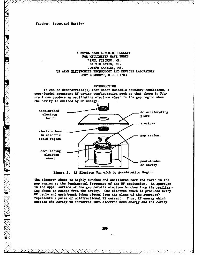
Fischer, Bates,and Hartley
A NOVEL BEAM BUNCHING CONCEPTFOR MILLIMETER WAVE TUBES
*PAUL FISCHER, MR.CALVIN BATES, MR.
JOSEPH HARTLEY, MR.US ARMY ELECTRONICS TECHNOLOGY AND DEVICES LABORATORY
FORT MONMOUTH, N.J. 07703
INTRODUCTIONIt can be demonstrated(l) that under suitable boundary conditions, a
post-loaded reentrant RF cavity configuration such as that shown in Fig-ure 1 can produce an oscillating electron sheet in its gap region whenthe cavity is excited by RF energy.
accelerated dc acceleratingelectron
bunch'-plate" '...bunch
aperture
electron bunchin electric gap regionfield region
oscillatingelectronsheet
post-loadedRF cavity
Figure 1. RF Electron Gun with dc Acceleration Region
The electron sheet is highly bunched and oscillates back and forth in thegap region at the fundamental frequency of the RF excitation. An aperturein the upper surface of the gap permits electron bunches from the oscil at-ing sheet to escape from the cavity. One electron bunch is produced everyRF cycle and each bunch (when viewed from the plane of the aperture)represents a pulse of unidirectional RF current. Thus, RF energy whichexcites the cavity is converted Into electron beam energy and the cavity
- --. ,-9,
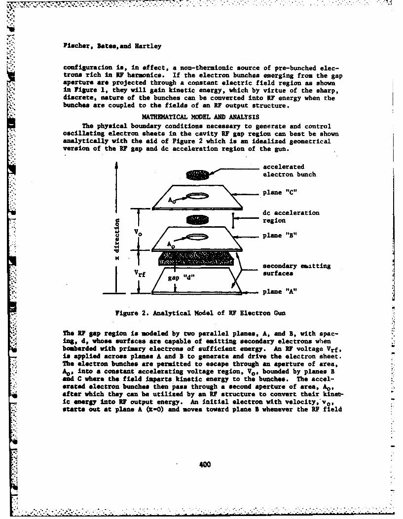
Fischer, Bates,and Hartley
configuracion is, in effect, a non-thermionic source of pre-bunched elec-trons rich in RF harmonics. If the electron bunches emerging from the gapaperture are projected through a constant electric field region as shownn Figure 1, they will gain kinetic energy, which by virtue of the sharp,
discrete, nature of the bunches can be converted into RF energy when thebunches are coupled to the fields of an RF output structure.
MATHEMATICAL MODEL AND ANALYSISThe physical boundary conditions necessary to generate and control
oscillating electron sheets in the cavity RI gap region can best be shownanalytically with the aid of Figure 2 which is an idealized geometricalversion of the RF gap and dc acceleration region of the gun.
acceleratedelectron bunch
plane "C"
r'- s~egionrett
dc acceleration
U VOplane ",B,
+ secondary enattingVrf surfaces
- L plane "A"
Figure 2. Analytical Model of RI Electron Gun
The RF gap region is modeled by two parallel planes, A, and B, with spac-ing, d, whose surfaces are capable of emitting secondary electrons whenbombarded with primary electrons of sufficient energy. An RF voltage Vrf,is applied across planes A and B to generate and drive the electron sheet.
.% The electron bunches are permitted to escape through an aperture of area,A0 , into a constant accelerating voltage region, Vo, bounded by planes Band C where the field imparts kinetic energy to the bunches. The accel-*rated electron bunches then pass through a second aperture of area, As,after which they can be utilized by an R structure to convert their kinet-ic energy into RF output energy. An initial electron with velocity,'vo,starts out at plane A (1-0) and moves toward plane B whenever the RP field
400
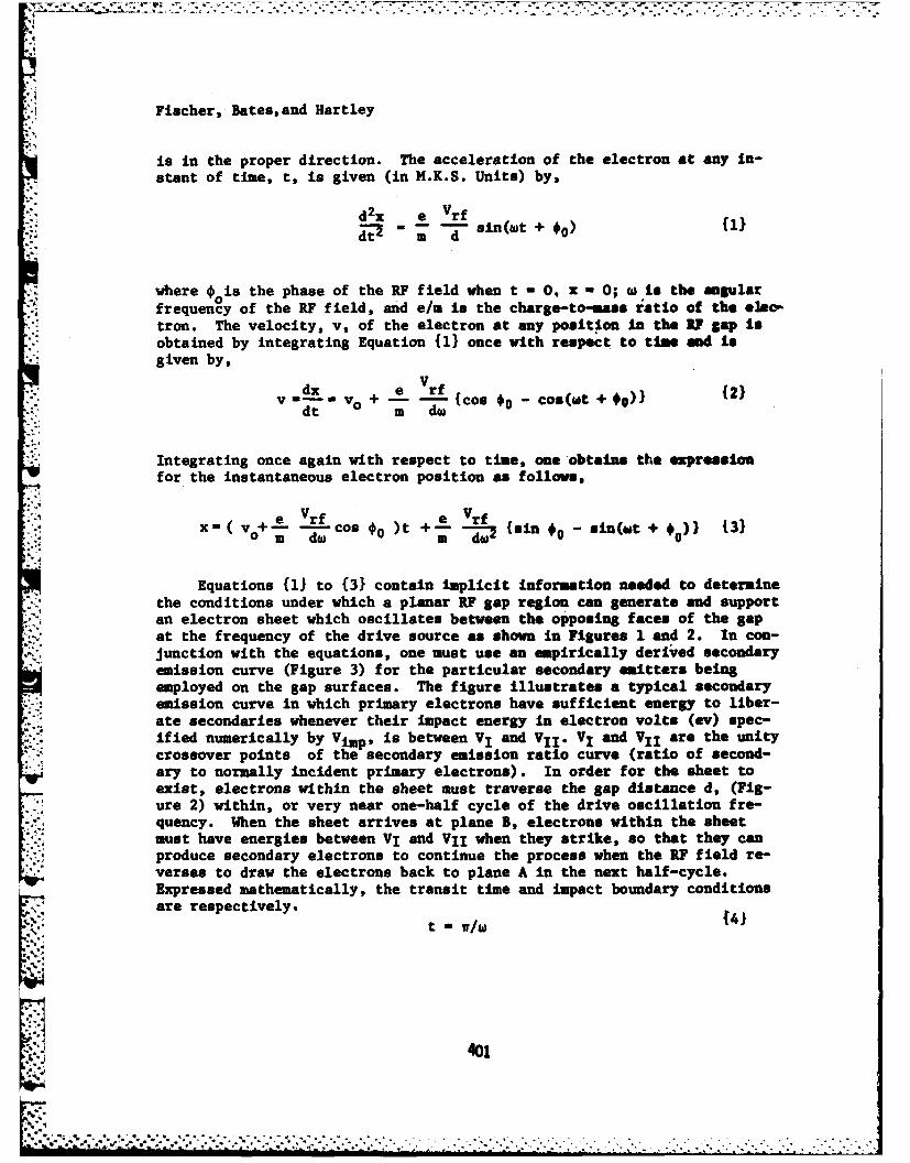
--.-.- ;.'- .c c C Ji C r . . ., _.. . . . - .* . . o . C a .- C' .. w °r - . - - - . . . . .- - "... L-.L- .o , . " " " o % , " °. ". . " • ° " • . -° .' - -o . -. ° . . . .. ° . -. , • " .
Fischer, Bates,and Hartley
is in the proper direction. The acceleration of the electron at any in-stant of time, t, is given (in M.K.S. Units) by,
d2x e Vrf0 m _ sin(awt +(i
where 0is the phase of the RF field when t - 0, x -0; w is the angularfrequency of the RF field, and e/m is the charge-to-mass ratio of the elec-tron. The velocity, v, of the electron at any position in the R7 gap is
4. obtained by integrating Equation {11 once with respect to time and is*given by,
dx e VrfV V + ( V con - cos(wt + 40))dt a dw 2
Integrating once again with respect to time, one obtains the ezpressionfor the instantaneous electron position as follows,
-x( v°L eVrf e Vrf
" m dw cos #0 )t + w- 7 (sin *0 - sin(ot + 0 13)
Equations {11 to (3) contain Implicit information needed to determinethe conditions under which a planar RF gap region can generate and supportan electron sheet which oscillates between the opposing faces of the gapat the frequency of the drive source as shown in Figures 1 and 2. In con-junction with the equations, one must use an empirically derived secondaryemission curve (Figure 3) for the particular secondary emitters beingemployed on the gap surfaces. The figure illustrates a typical secondaryemission curve in which primary electrons have sufficient energy to liber-ate secondaries whenever their impact energy in electron volts (ev) spec-ified numerically by Vimp, is between V, and VIZ. V, and VII are the unitycrossover points of the secondary emission ratio curve (ratio of second-ary to normally incident primary electrons). In order for the sheet toexist, electrons within the sheet must traverse the gap distance d, (Fig-ure 2) within, or very near one-half cycle of the drive oscillation fre-quency. When the sheet arrives at plane B, electrons within the sheetmust have energies between VI and VII when they strike, so that they canproduce secondary electrons to continue the process when the RF field re-verses to draw the electrons back to plane A in the next half-cycle.
Expressed mathematically, the transit time and impact boundary conditionsare respectively,
t - 7/L
U 401
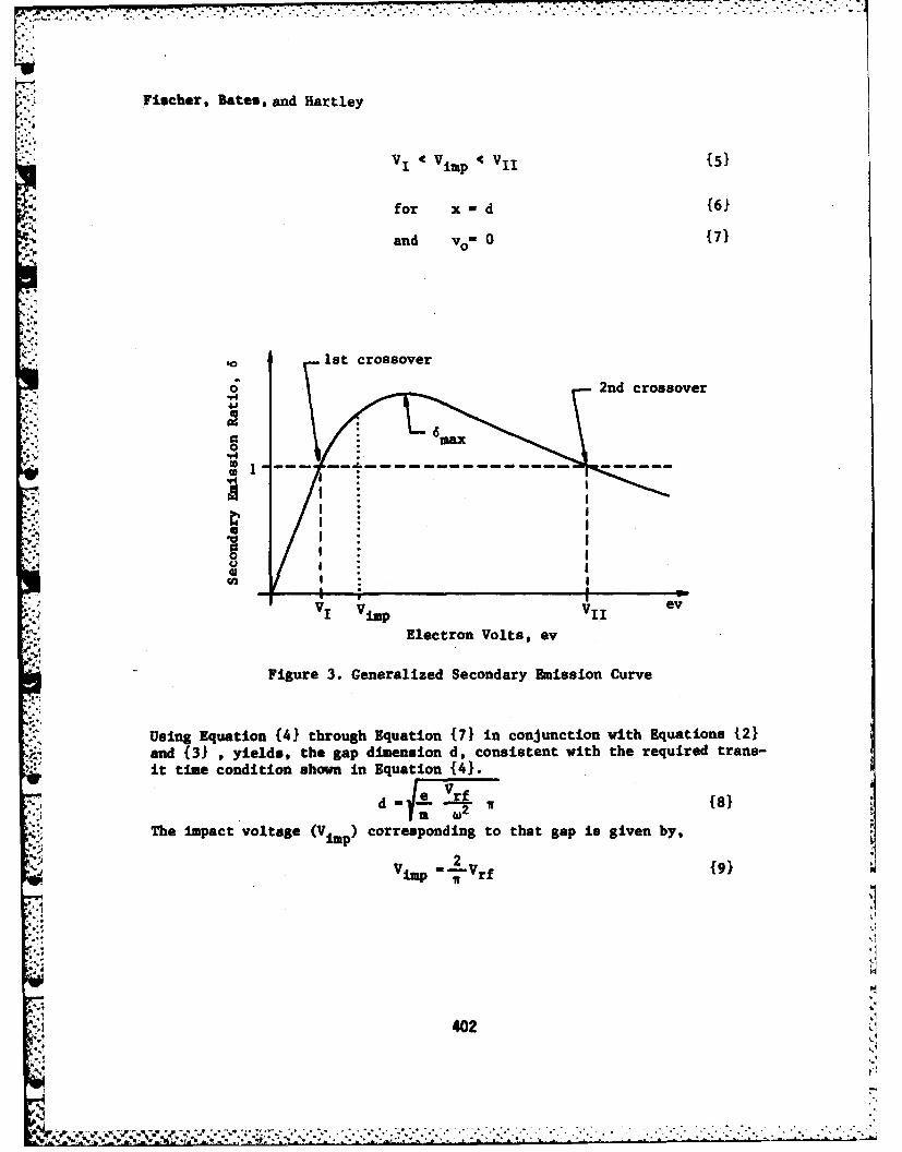
Fischer, Bates, and Hartley
for xmd (6J
and vo 0 (71
Is cosoe
1std crossover
0
0e- - im ----- -- - -
Electron Volts, ev
Figure 3. Generalized Secondary Emission Curve
Using Equation {41 through Equation (71 in conjunction with Equations t.21r and (31 , yields, the gap dimension d, consistent with the required trans-
it time condition shown in Equation (41.
d (81
The Impact voltage (Vi) coreponding to that gap is given by,
Vimp "h~rf (91
A 402
Fischer, Bates, and Hartley
Vjmp can be chosen independently from the experimental secondary emissioncurve (Figure 3); in practice it is preferable to pick Vimp at the peak,(6 max), of the curve so that the maximum number of secondary electrons areobtained at impact each half-cycle. Once Vimp is specified, Vrf is deter-mined by Equation (91. The required Vrf is a function of the cavity (Fig-ure 1) gap shunt impedance Rsh, and input drive power Pd, where,
Pd m Vrf2 {101Rsh
Vrf, therefore, can be obtained by suitable cavity design for Rsh or ad-Justment of the drive power, Pd or both. Since the shunt impedance anddrive power can be chosen independently of frequency (2), Vrf is independ-ent of frequency. Furthermore, the physical phenomenon of electron bunch-
. ing is not dependent on frequency, but is determined by the phase of the: ,electron leaving one surface, and the phase and energy with which it* 'strikes the opposite surface. The electron bunching process occurs as a
result of the phase and energy selection of electrons existing in the gapregion. Thus, a scaled experimental model (for example 5 Gigahertz (GHz))can be designed and built to verify the foregoing analysis for millimeterwave lengths. Once the shunt impedance and drive power are specified toproduce the required RF voltage (Vrf), the gap spacing (d) is determinedby Equation {8} for any desired drive frequency, W.
The cyclic electron build-up and bunching process described in theforegoing analysis is a special case of the secondary electron resonancephenomenon (also called multipactor) extensively described in the scien-tific literature (see, for example, Reference 3). Equations 81 and 9}which specify the gap dimension and the corresponding electron impactenergy (Vimp) were derived for an initial electron velocity and departuretime of zero. In actuality, electrons are emitted over a range of depar-ture times (departure angle) and arrive at the opposite gap face over arange of arrival times (conduction angle). The departure and arrival timesare normally clustered about t - 0 and t - /w, respectively, for practicalcases. In addition, the emitted electrons have initial velocities corre-sponding to energies of 0 to 30 ev (4) with the maximum number of electronsemitted at approximately 2-5 ev. Iterative calculations using Newton'smethod (5), for Equations {21 and {31, show that electrons having initialenergies of up to 5 ev, will have departure and arrival times which clus-ter about t - 0 and t - ir/w respectively. The increased initial veloci-ties will cause corresponding increases in departure and conduction angles.Experimental devices to be discussed in this report employ a gap spacingof 0.020 inches (0.508mm), with surfaces of either silver or copper (seeReference 4 for experimental secondary emission curves). For this gap,calculations yield values of approximately 30 degrees for the departureand conduction angles.
403
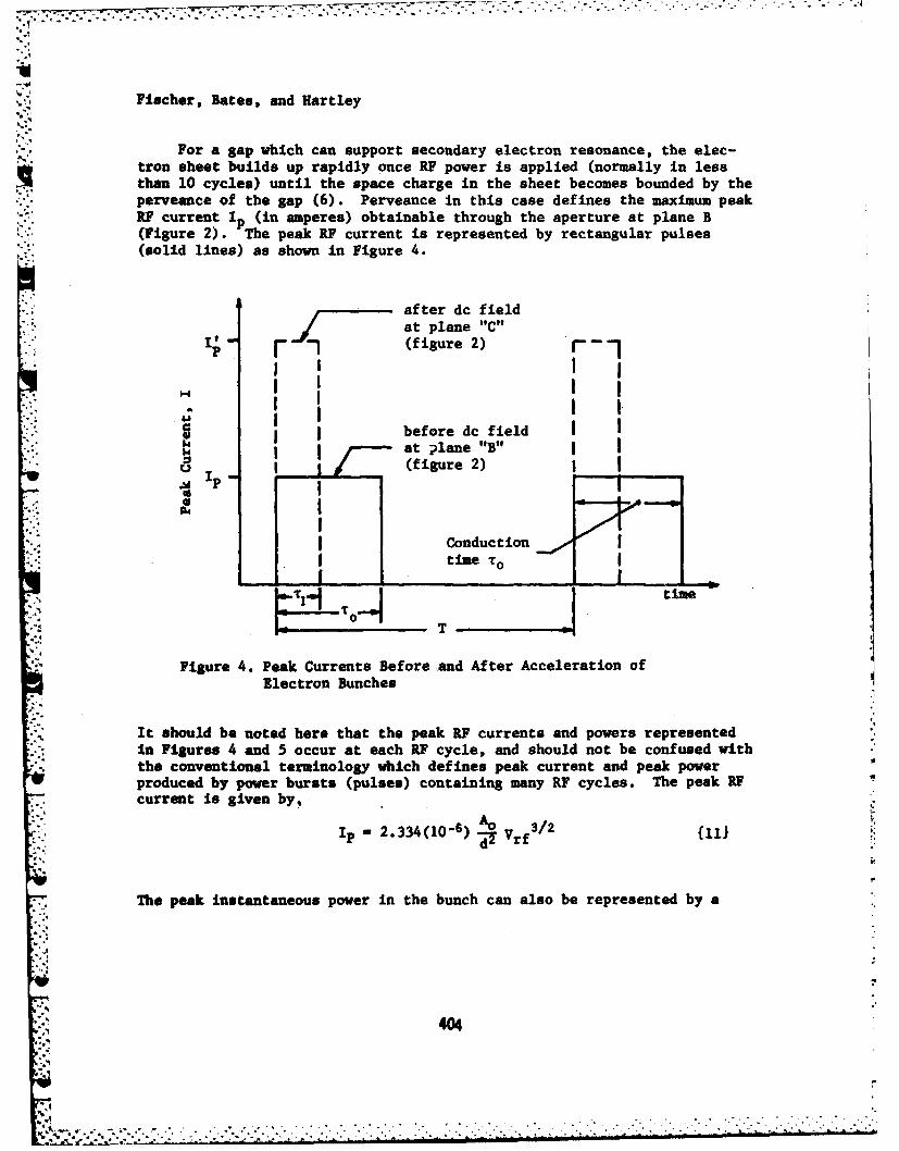
Fischer, Bates, and Hartley
For a gap which can support secondary electron resonance, the elec-tron sheet builds up rapidly once RF power is applied (normally in lessthan 10 cycles) until the space charge in the sheet becomes bounded by theperveance of the gap (6). Perveance in this case defines the maximum peakRF current Ip (in amperes) obtainable through the aperture at plane B(Figure 2). The peak RF current is represented by rectangular pulses(solid lines) as shown in Figure 4.
"J/ after dc fieldj 7at plane "C"• Ip t (f igure 2) r
I I I
before dc field Iat ?lane "B"
(figure 2)
. Conduction•I time To
time,'T 0_ T .• =
Figure 4. Peak Currents Before and After Acceleration ofElectron Bunches
It should be noted here that the peak RF currents and powers representedin Figures 4 and 5 occur at each RF cycle, and should not be confused withthe conventional terminology which defines peak current and peak powerproduced by power bursts (pulses) containing many RF cycles. The peak RFcurrent Is given by,
A..I - 2.334(10 6) 3/2'1)
The peak instantaneous power in the bunch can also be represented by a
404
........ ...... ..
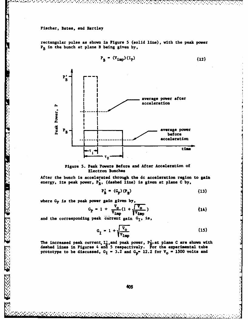
Fischer, Bates, and Hartley
rectangular pulse as shown in Figure 5 (solid line), with the peak powerPin the bunch at plane B being given by,
- (Vimp)(Ip (121
I I average power afteracceleration
I...... 10101o I
40 B T average powerI4 B , before............................ ... acceleration
time-
Figure 5. Peak Powers Before and After Acceleration ofElectron Bunches
After the bunch Is accelerated through-the dc acceleration region to gainenergy, its peak power, Pj, (dashed line) is given at plane C by,
-B (G,) (P B) (13)
where Gp is the peak power gain given by,
A VmVimp V
and the corresponding peak current gain G1 9 is,
G 1+I_+ (151
The increased peak current I' and peak power, PB, at plane C are shown withdashed lines in Figures 4 QnS5 respectively. For the experimental tubeprototype to be discussed, G, - 3.2 and Gp-m 12.2 for V0 1500 volts and
405
-V4 ~ .:.~x:-.*.----.--.---
~~~~..:'.- - :.." "..........-' "" "........ ...... *.. . .
'U
4. Fischer, Bates, and Hrtley
Via - 300 volts (for copper). Thus, a substantial increase in the kinet-ic energy of the bunches can be obtained with a moderate accelerating dcvoltage. The average power gain Gavp produced by the dc fields is,
V1Gavp Vimp +161
and for the prototype tube Gavp - 5.3. Figure 5 also indicates that theaverage power is increased after acceleration (dotted lines).
The peak currents shown in Figure 4 can be represented by a Fourierseries (7). For the purposes of this paper, we are interested only inthe fundamental component of the RF current at plane C and its amplitudeI, is given by, I I G sinr L
1 .P IT (171
where TI, is the pulse width of the current at plane C, and T is theperiod of the fundamental IF drive. The ratio of the pulse width T1 atplane C, to the pulse width,T0 , at plane B is,
{181+I Vim
and shows the effect of the dc accelerating field (Vo ) on the pulse widthsof instantaneous current and power. Neglecting RP circuit losses, one canshow that the maximum RF power gain Grf (with respect to the fundamentalcomponent) achieveable with the electron bunches is,
Grf + 119}
and the maximum efficiency, r ,.2s,
:;...I + 2ViME
0
Thus, the maximum limitations of RI power gain and efficiency (neglectingthe HP losses in the RP input and output structures) with the gun/bunchingconfiguration as shown in Figures I and 2, are functions of the impactvoltage (Vimp) and the dc accelerating voltage (Vo). From Equations (191and (201, it follows that in order to optimize gain and efficiency, onemust minimize Vimp and maximize Vo . Vimp in practice for presently use-able secondary emitting materials (copper, silver, gold, platimm, magne-sia-gold-cermets, etc.) is between 35 and 1000 ev. Power-supply/modulator,voltage breakdown, and electron de-bunching considerations affect the
'406
"42
,; :.". ... "."- .: " .:" ; , ;.-'-". .'" ".' .'-.' ".- .-: ."-."- ". .. ".... ." "-.. .". .'.. . .'-. .,...--.. .-.- ".".-.. .-.. . . .-.-.. . - i-- '-. .."
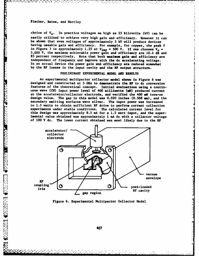
: : ic;, ,: ,, , ,ii. .. ,; .. . .................. ...... ....... . .. . . : -
Fischer, Bates, and Hartley
choice of Vo . In practice voltages as high as 25 kilovolts (kV) can be
easily utilized to achieve very high gain and efficiency. However it canbe shown that even voltages of approximately 5 kV will produce deviceshaving useable gain and efficiency. For example, for copper, the peak 6in Figure 3 is approximately 1.25 at Vip - 500 V. If one chooses Vo -5,000 V, the maximum achievable power gain and efficiency are 10.4 dB and83 percent respectively. Note that both maximum gain and efficiency areindependent of frequency and improve with the dc accelerating voltage.In an actual device the power gain and efficiency are reduced somewhatby the RI losses in the input cavity and the RI output structure.
PRELIMINARY EXPERIMENTAL MODEL AND RESULTSAn experimental multipactor collector model shown in Figure 6 was
designed and constructed at 5 GHz to demonstrate the RF to dc conversionfeatures of the theoretical concept. Initial evaluations using a contin-uous wave (CW) input power level of 400 milliwatte (WW) produced currentat the accelerator/collector electrode, and verified the 400 UW turn-ondesign value. The gap in this model was 0.020 inches (0.508 mm), and thesecondary emitting surfaces were silver. The input power was increasedto 1.5 watts to obtain sufficient RI drive to perform current collectionexperiments under stable conditions. The calculated current level forthis design was approximately 8.5 mA for a 1.5 watt input, and the exper-imental value obtained was approximately 1 mA dc with a collector voltageof 100 V dc. The lower current obtained was most likely due to the RF
accelerator/collectorelectrode
envelopeRI
coupli n post-loadediris Fcvt
gap region RI cavity
7Figure 6. Experimental Multipactor Collector Model
407
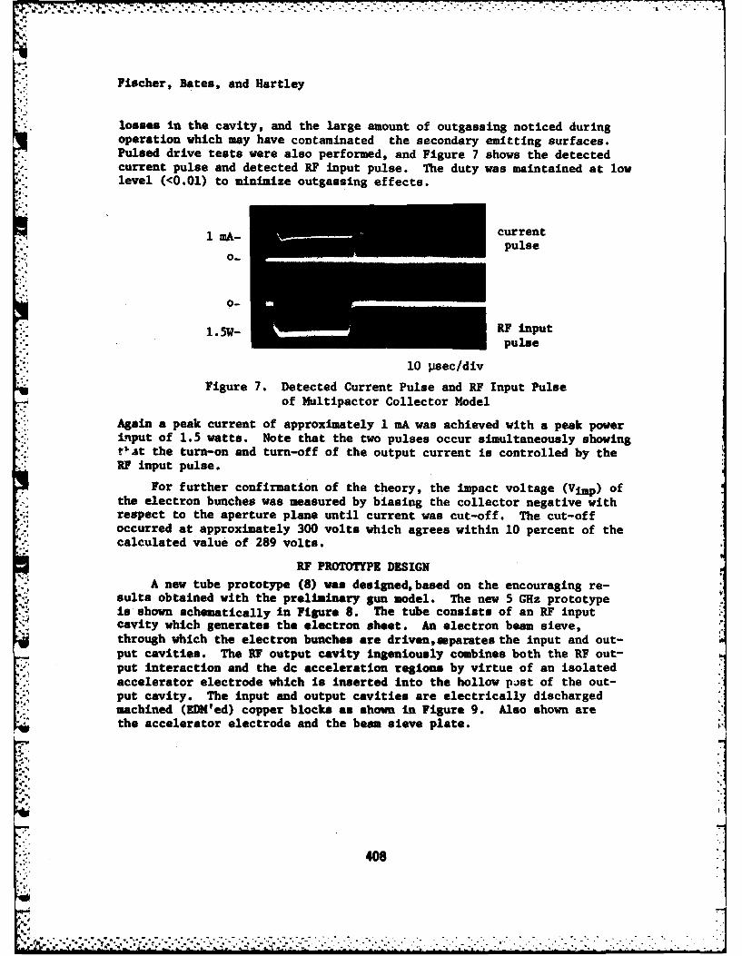
Fischer, Bates, and Hartley
losses in the cavity, and the large amount of outgassing noticed duringoperation which may have contaminated the secondary emitting surfaces.Pulsed drive tests were also performed, and Figure 7 shows the detectedcurrent pulse and detected RF input pulse. The duty was maintained at lowlevel (<0.01) to minimize outgassing effects.
1 mA- currentpulse
0-
1.5W- RI input
pulse
10 psec/div
Figure 7. Detected Current Pulse and RF Input Pulseof Multipactor Collector Model
Again a peak current of approximately 1 mA was achieved with a peak powerinput of 1.5 watts. Note that the two pulses occur simultaneously showingV' t the turn-on and turn-off of the output current is controlled by theRF input pulse.
For further confirmation of the theory, the impact voltage (Vimp) ofthe electron bunches was measured by biasing the collector negative withrespect to the aperture plane until current was cut-off. The cut-offoccurred at approximately 300 volts which agrees within 10 percent of thecalculated value of 289 volts.
RF PROTOTYPE DESIGN
A new tube prototype (8) was designed, based on the encouraging re-sults obtained with the preliminary Sun model. The new 5 GHz prototypeis shown schematically in Figure 8. The tube consists of an RF inputcavity which generates the electron sheet. An electron beam sieve,through which the electron bunches are driven,mparates the input and out-put cavities. The IF output cavity ingeniously combines both the RF out-put interaction and the dc acceleration regions by virtue of an isolatedaccelerator electrode which is inserted into the hollow pist of the out-put cavity. The input and output cavities are electrically dischargedmachined (EDH'ed) copper blocks as shown in Figure 9. Also shown are %the accelerator electrode and the beam sieve plate.
; . .40
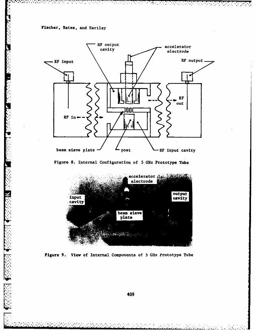
Fischer, Bates, and Hartley
RF output acceleratorcavity electrode
EF input otu
RF
ooutRP in.-
beam sieve plate post RF input cavity
Figure 8. Internal Configuration of 5 GHz Prototype Tube
- } outt;;. nut avty
-;... ,cavity
r:' : beam sieve ro plate
L Figure 9. View of Internal Components of 5 GHz Prototype Tube
409
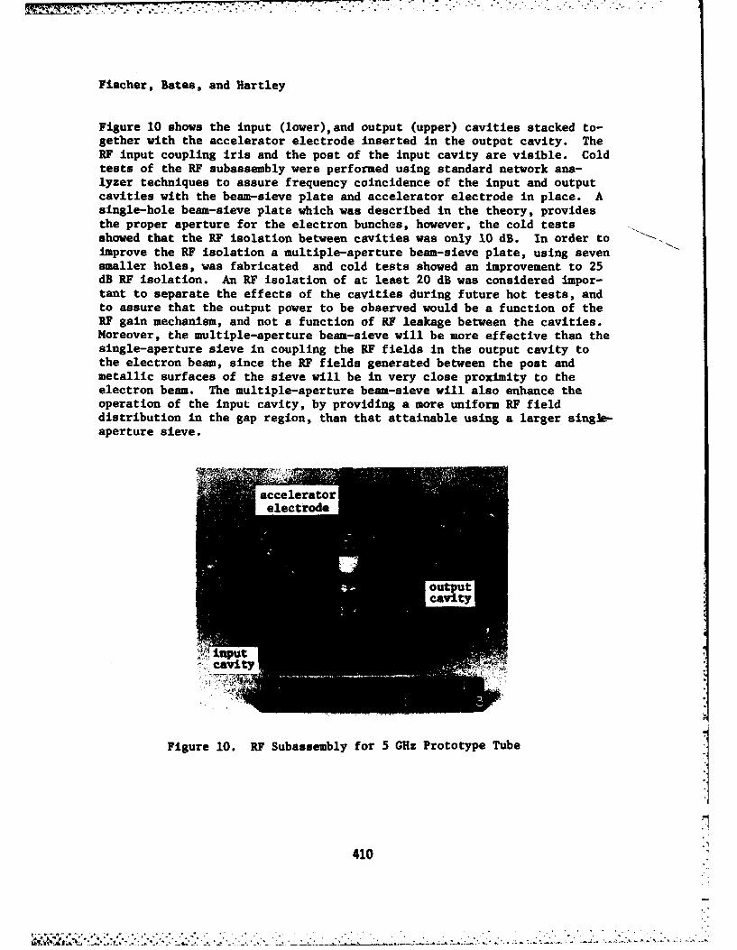
Fischer, Bates, and Hartley
Figure 10 shows the input (lower),and output (upper) cavities stacked to-gether with the accelerator electrode inserted in the output cavity. TheRF input coupling iris and the post of the input cavity are visible. Coldtests of the RF subassembly were performed using standard network ana-lyzer techniques to assure frequency coincidence of the input and outputcavities with the beam-sieve plate and accelerator electrode in place. Asingle-hole beam-sieve plate which was described in the theory, providesthe proper aperture for the electron bunches, however, the cold testsshowed that the RF isolation between cavities was only 10 dB. In order toimprove the RF isolation a multiple-aperture beam-sieve plate, using sevensmaller holes, was fabricated and cold tests showed an improvement to 25dB NP isolation. An RF isolation of at least 20 dB was considered impor-tant to separate the effects of the cavities during future hot tests, andto assure that the output power to be observed would be a function of theRF gain mechanism, and not a function of RF leakage between the cavities.Moreover, the multiple-aperture beam-sieve will be more effective than thesingle-aperture sieve in coupling the "F fields in the output cavity tothe electron beam, since the RF fields generated between the post andmetallic surfaces of the sieve will be in very close proximity to theelectron beam. The multiple-aperture beam-sieve will also enhance theoperation of the input cavity, by providing a more uniform RF fielddistribution in the gap region, than that attainable using a larger sing]e-aperture sieve.
I acceleratorelectrode
Iinput-icavity ?
Figure 10. RF Subassembly for 5 GHz Prototype Tube
410
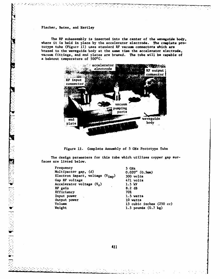
Fischer, Bates, and Hartley
The RF subassembly is inserted into the center of the waveguide body,where it is held in place by the accelerator electrode. The complete pro-totype tube (Figure 11) uses standard RF vacuum connectors which arebrazed to the waveguide body at the same time the accelerator electrode,vacuum fittings, and end plates are brazed. The tube will be capable ofa bakeout temperature of 5000C.
"acceleratorFie e. plectre RF outputb
fae r isted belo.': eltrd
Frequenyc5 Gae
RF input
vacuum
Outputpoweru 0 watt
port.................... n
i'-'end waveguide'.i . .Plate body
Figure 11. Complete Assembly of 5 GHz Prototype Tube
> The design parameters for this tube which utilizes copper gap sur-. faces aelisted below.
;:Frequency 5 GHz• ":,Multipactor gap, (d) 0.020" (0.5- ): Electron impact, voltage (Vimp ) 300 volts,."-'Gap RF voltage 471 volts:Accelerator voltage (Vo ) 1.5 kV
SRF gain 8.2 dB,':.'Efficiency 70%: iInput power 1. 5 watts:-.Output power 10 watts-''Volume 15 cubic inches (250 cc)" Weight 1.5 pounds (0.7 kg)
ili: ;411
7----4
Fischer, Bates, and Hartley
This feasibility prototype has been designed and fabricated to demon-strate the formation of the electron bunches, and the gain mechanismgenerated by interaction with the RF fields. Future multi-stage modelsdesigned around the concept will demonstrate enhanced capabilities forspecific Army system application.
CONCLUSIONS
A unique electron beam bunching concept has been presented, analyzed,and applied to the development of a novel tube approach. The analysisprovides a design base for a new class of millimeter wave tubes. Thesetubes will be compact, lightweight, reliable, and low cost due to thesimplicity of design and construction in comparison to conventionalthermionic tubes with magnets. Furthermore, the analysis shows that use-ful RF gain and efficiency can be achieved at moderate accelerator volt-ages, which makes possible the use of simplified, low cost, lightweight,power supplies and modulators.
Theoretical considerations have been confirmed by evaluation of anexperimental multipactor collector model. Furthermore, the results havedemonstrated that the electron bunching can be generated and controlledby low RF drive (less than 1 watt), and that the currents generated areuseful for new tube approaches. Although experiments were conducted at5 GHz, the results are applicable for devices operating at millimeter wavefrequencies.
A 5 GHz prototype tube design has been formulated, and componentparts for the tube have been machined and cold-tested. The tube is pres-ently being assembled for subsequent processing and evaluation. It isexpected that this simplified, two-cavity design will demonstrate usefulgain and efficiency, and provide the technology base for developing newtube ptototypes for Army millimeter wave system applications.
REFERENCES
(1) C. Bates et. al., "Multipactor Electron Gun for Millimeter WaveTubes,"IEDM Technical Digest, pp 339-343, Dec 1981.
* (2) T. Moreno, M Transs Daa, McGraw-Hill Book Co.,Inc., First Edition, pp 228-230, 1948
(3) A. J. Hatch, "Electron Bunching in the Multipacting Mechanism of. High-Frequency Discharge," Journal of Applied Physics, Vol. 32,
No. 6, pp 1086-1092, June 1961
(4) H. Bruining, Physics and Applications of Secondary Electron Emission,Pergamon Press, Ltd., First Edition, pp 27-31, 104-107, 1954
412
. -. . . .,-. .. .,.,.... ..... • .. . .. .. .. ..- .-

Fischer, Bates, and Hartley
(5) D. McCracken, FORTRAN With Engineering Applications, John Wiley &
Sons, Inc., pp 44-52, 1967
(6) W. J. Gallagher, "The Multipactor Effect," IEEE Transactions on
Nuclear Science, Vol. NS-26, No. 3, pp 4280-4282, June 1979
(7) S. Goldman, Frequency Analysis Modulation and Noise, McGraw-Hill,pp 25-27, 1948
(8) C. Bates, "Multipactor Beam Amplifier," Invention Disclosure, Docket
No. 2447, filed Hay 1981
413
'41
FRIEDMAN, CA1PANA & YERGEY
NEW VIEWPOINTS IN MASS FILTER DESIGN
*MELVIN H. FRIEDMAN, PhD**1. US ARMY MOBILITY EQUIPMENT R&D COMMAND, FORT BELVOIR, VA 22060
JOSEPH E. CAMPANA, PhD* US NAVAL RESEARCH LABORATORY, WASHINGTON, DC 20375
ALFRED L. YERGEY, PhDNATIONAL INSTITUTES OF HEALTH, BETHESDA, MD 20205
1. INTRODUCTIONThe quadrupole mass filter (QMF) is ubiquitous in military and
civilian mass spectrometry laboratories. This instrument is used bychemists to determine the mass distribution associated with a sample. Asillustrated in figure 1, a QKF has four pole pieces and each of these iscarefully shaped to follow the equation of a hyperbola i.e. with the co-ordinate system ehown the equations of the pole pieces are given by(X2 - y2) - ±r!. In a typical QMF, r. and t are .28 cm and 15 cmrespectively (1). Detailed analysis shows (2) that mass filtering actionis achieved by Imposing a voltage difference 0 - &DC - &AC cos wtbetween adjacent electrodes. The driving frequency v - (w/2n) istypically 2.5 MHz. The voltages * and * are refered to as the DCand AC components of the applied vKtage r*pectively. The result ofdetailed analyses (1,2) is that the mass resolution of a QMF is determined
*'. by the ratio */I* while the absolute magnitude of the voltages 0 DC and",Cdetermine KRe fiss of the ion which sucessfully traverses the lengthoTthe instrument. In the typical operation of the instrument (1) 0and *AC are allowed to vary while their ratio is held constant and t9enumber of ions which sucessfully traverse the filter are recorded.
The mass resolving power of a mass filter at mass m is defined bym/Am where Am is a measure of the smallest difference in mass at mass mthat can be detected by the instrument at a specified valley (e.g. 102peak height) between peaks of equal heights. The transmission of a massfilter tuned to mass m is defined as the ratio of the number of ions withmass m injected into the mass filter to the number which arrive at thedetector. It would be desirable for a QMF to have high resolving powerand high transmission. Unfortunately, these are conflicting requirementsand the improvement in one of these parameters results in a degradationof the other parameter.
.41- ". 415
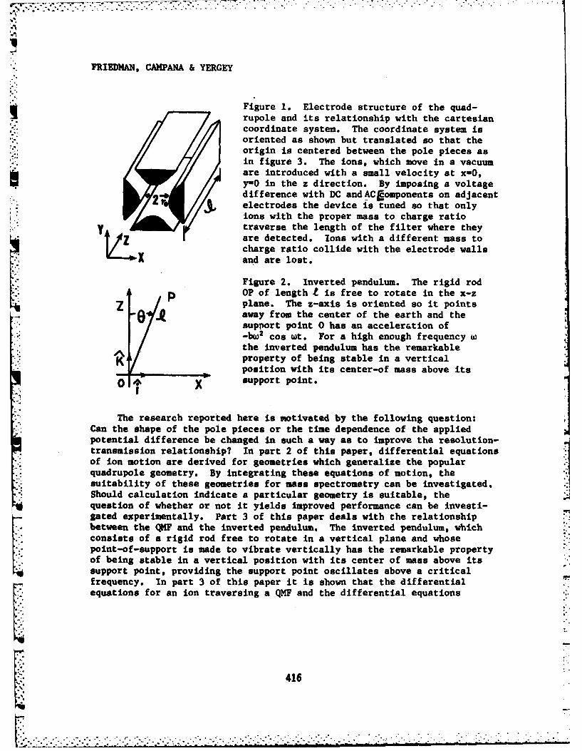
FRIEDMAN, CAMPANA & YERGEY
Figure 1. Electrode structure of the quad-rupole and its relationship with the cartesiancoordinate system. The coordinate system isoriented as shown but translated so that theorigin is centered between the pole pieces as
V in figure 3. The ions, which move in a vacuumare introduced with a small velocity at x-O,y=O in the z direction. By imposing a voltagedifference with DC andACcomponents on adjacent23. electrodes the device is tuned so that onlyions with the proper mass to charge ratio
Ytraverse the length of the filter where theyare detected. Ions with a different mass to
Icharge ratio collide with the electrode wallsand are lost.
Figure 2. Inverted pendulum. The rigid rod- OP of length t is free to rotate in the x-z
plane. The z-axis is oriented so it pointsaway from the center of the earth and thesupport point 0 has an acceleration of-bw2 cos wt. For a high enough frequency wthe inverted pendulum has the remarkable
S property of being stable in a vertical
'"___ position with its center-of mass above its
A . x support point.
The research reported here is motivated by the following question:Can the shape of the pole pieces or the time dependence of the appliedpotential difference be changed in such a way as to improve the resolution-transmission relationship? In part 2 of this paper, differential equationsof ion motion are derived for geometries which generalize the popularquadrupole geometry. By integrating these equations of motion, thesuitability of these geometries for mass spectrometry can be investigated.Should calculation indicate a particular geometry is suitable, thequestion of whether or not it yields improved performance can be investi-gated experimentally. Part 3 of this paper deals with the relationshipbetween the QMF and the inverted pendulum. The inverted pendulum, whichconsists of a rigid rod free to rotate in a vertical plane and whosepoint-of-support is made to vibrate vertically has the remarkable propertyof being stable in a vertical position with its center of mass above its v,1
support point, providing the support point oscillates above a criticalfrequency. In part 3 of this paper it is shown that the differentialequations for an ion traversing a QMF and the differential equations
[ 416
• . . . . .-- , .
FRIEDMAN, CAMPANA & YERGEY
describing the motion of an inverted pendulum can be cast into the sameform. In this way the inverted pendulum is shown to be a mechanical analogof the QMF. This aspect of the work is significant for three reasons:1) The motion of an ion as it traverses a QMF cannot be physically seen.By observing the motion of an inverted pendulum one may better appreciatethe subtleties involved in the way a quadrupole works and perhaps obtain abetter sense of what is happening in this device. This may be of value tothe person who tries to design a better mass filter. 2) The invertedpendulum has pedagogical value for explaining the operation of a Q4F tostudents and has already been used for this purpose by one of the authors(A.L.Y). 3) By showing that the inverted pendulum and QMF are relatedsubjects, it is possible that studies on one of them may shed light onthe other.
The inverted pendulum has been described by several authors (3-10).Corben and Stehle (3) have modeled the inverted pendulum as a rigid rodwhile Landau and Lifshitz (4) have modeled it as a point mass attached toa rigid massless rod. Kapitza (5) has discussed the case of the pendulumwhen the amplitude of the sinusoidal oscillation of the suspension pointis small in comparison to the length of the pendulum. He has also reported
- what appears to be the first operative pendulum with an oscillatingsupport point (normal and inverted). Kalmus (6) has discussed the theoryof the inverted pendulum with triangular excitation of the support point,and has reported an operative inverted compound pendulum. Mitchell (7)has applied a method of averaging to find the stability of an invertedpendulum for small amplitude high frequency oscillation, and Howe (8) hasdescribed a theory for the stability of an inverted pendulum driven byoscillations of a random nature. A square-wave model of the invertedpendulum has been recently described by Yorke (9). In a previouspublication (10), Friedman et al. have observed that the inverted pendulumis a mechanical analog of the QMF.
Partial derivations of the differential equations for ion motion in aQMF are given by Campana (1) and also by Dawson (2). A derivation (start-
* -.. ing from the Lorentz force law and the most general form of the Maxwellequations) for ion motion in multipole fields with a discussion ofvarious approximations has been given by Friedman et al. (11).
2. ION MOTION IN MULTIPOLE FIELDSa. Fundamental physics 2L ion motion. The force on an ion with
chargee moving with velocityv through space in which there is an electricfield E and a magnetic field B is given by the Lorentz force law
-1- 4. 4.F - e(E + v x B). (1)
The differential equation which describes the motion of an ion through afield is obtained from Newton's law of motion
417
' , ;'/' ;,''/:'.'':?-'-:.°: '..2.-i-;, ...--: .. -i,'. ". .." -: .,: i .. -:. • ..-. .:- -i.-
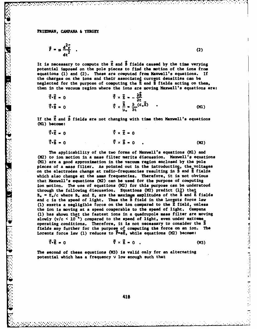
FRIE DA, CAMPANA & YURGEY
I%2-1°r
- . (2)dt 2
It is necessary to compute the E and B fields caused by the time varyingpotential imposed on the pole pieces to find the motion of the ions fromequations (1) and (2). These are computed from Maxwell's equations. Ifthe charges on the ions and their associatei currt densities can beneglected for the purpose of computing the E and T fields acting on them,then in the vacuum region where the ions are moving Maxwell's equations are:
4.
at 4 .
B a (e.E) *(1)
If the E and B fields are not changing with time then Maxwell's equations(Ml) become:
.xemO
0 x.B (M2)
The applicability of the two forms of Maxwell's equations (1l) and(M42) to ion motion in a mass filter merits discussion. Maxwell's equations(41) are a good approximation in the vacuum region enclosed by the polepieces of a mass filter. As pointed out in the introduction, the-voltageson the electrodes change at radio-frequencies resulting inB and E fieldswhich also change at the same frequencies. Therefore, it is not obviousthat Maxwell's equations (M2) can be used for the purpose of computingion motion. The use of equations (12) for this purpose can be understoodthrough the following discussion. Equations (42) predict (l) thajBe - E./c where B. and E. are the axisma amplitudes of the and E fieldsand c is the speed of light. Thus the B field in the Lortntz force law(1) exerts a negligible force on the ion compared to the E field, unlessthe ion is moving at a speed comparable to the speed of light. Campana(1) has shown that the fastest ions in a quadrupole mass filter are movingslowly (v/c < 10-4) compared to the speed of light, even under extremeoperating conditions. Therefore, it is not necessary to consider thefields any further for the purpos) of computing the force on an ion. TheLorentz force law (1) reduces to ate, while equations (M2) become:
Th0-o x o . (M3)
The second of these equations (13) is valid only for an alternatingpotential which has a frequency v low enough such that
418
A.?.... . ............,... .... ?'.-....-.-.. ..... ,_, ., - _. __-..... . * _ .
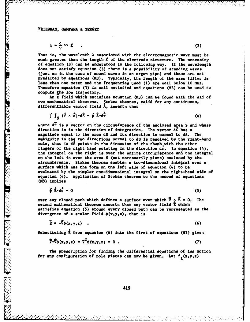
FRIEDM4AN, CAMPANA & YERGEY
=5 .>> . (3)V
That is, the wavelenth X associated with the electromagnetic wave must bemuch greater than the length L of the electrode structure. The necessityof equation (3) can be understood in the following way. If the wavelengthdoes not satisfy equation (3) there is a possibility of standing waves(just as in the case of sound waves in an organ pipe) and these are notpredicted by equations (N3). Typically, the length of the mass filter isless than one meter and the frequencies used (1) are well below 10 MHz.Therefore equation (3) is well satisfied and equations (M3) can be used tocompute Jhe ion trajectory.
An E field which satisfies equation (143) can be found with the aid oftwo mathematical theorems. §tokes theorem, valid for any continuous,differentiable vector field A, asserts that
f. fS x Aodr (4)
where dr is a vector on the circumference of the enclosed a ea S and whosedirection is in the direction of integration. The vector dS has amagnitude equal to the area dS and its direction is normal to dS. Theambiguity in thS two directions normal to dS is resolved by the right-handrule, that is dS points in the direction of the thumb with the otherfingers of the right hand pointing in the direction dr. In equation (4),the integral on the right is over the entire circumference and the integralon the left is over the area S (not necessarily plane) enclosed by thecircumference. Stokes theorem enables a two-dimensional integral over asurface which has the form on the left side of equation (4) to beevaluated by the simpler one-dimensional integral on the right-hand side ofequation (4). Application of Stokes theorem to the second of equations
-W: (143) implies
Eedr - 0 (5)
over any closed path which defines a surface over which x E 0. Thesecond mathematical theorem asserts that any vector field I whichsatisfies equation (5) around every closed path can be represented as thedivergence of a scalar field *(x,yz), that is
E , -1,(x,y,z) . (6)
Substituting E from equation (6) into the first of equations (43) gives
-04(xy~z) " V2*(xyz) - 0 . (7)
The prescription for finding the differential equations of ion motionfor any configuration of pole pieces can now be given. Let f1 (xytz)
L419
, : ,- +.. , .+..+ -- +....'+. . +. +. . . . . . . .+..-- - . +. .+ . . _., --... +. +... . .+. +
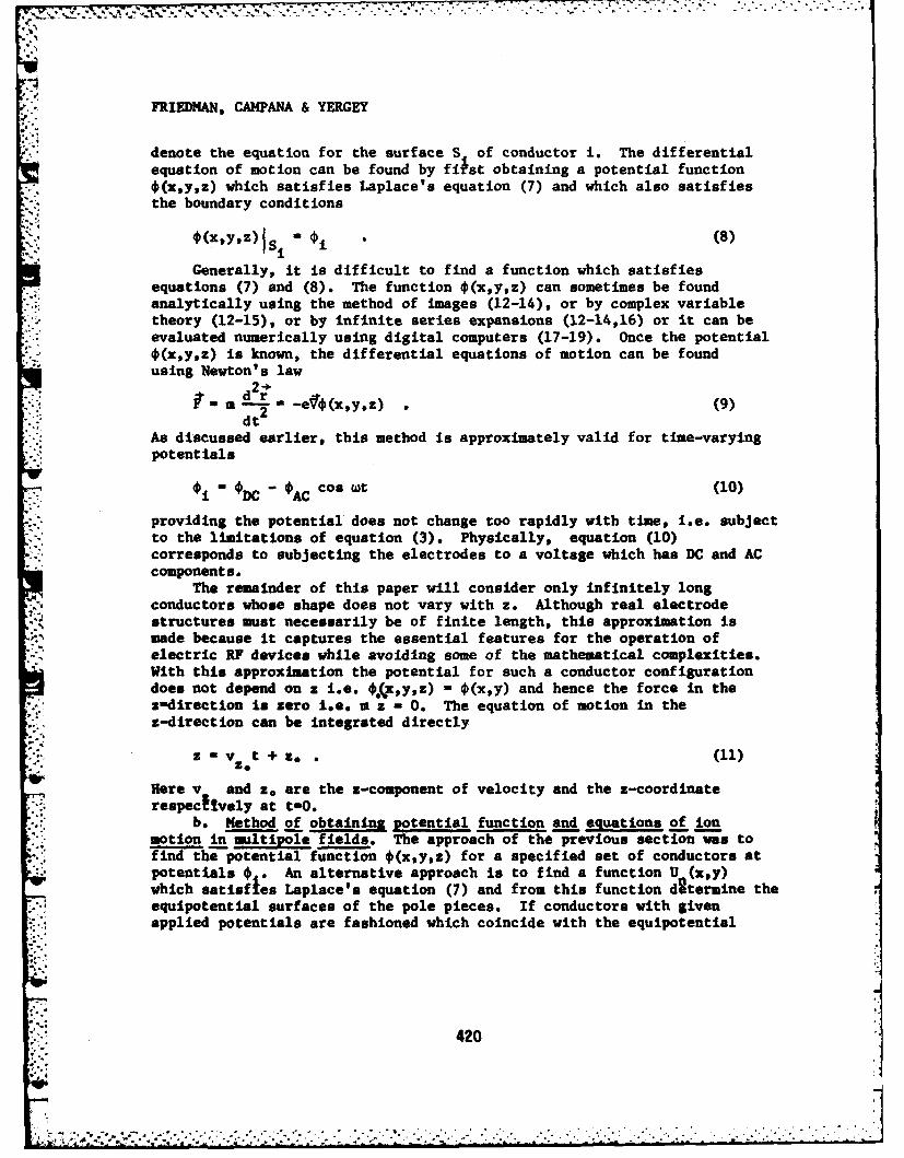
FRIEDMAN, CAMPANA & YERGEY
denote the equation for the surface Si of conductor i. The differentialequation of motion can be found by first obtaining a potential function*(x,y,z) which satisfies Laplace's equation (7) and which also satisfiesthe boundary conditions
Is
(
Generally, it is difficult to find a function which satisfiesequations (7) and (8). The function O(xy,z) can sometimes be foundanalytically using the method of images (12-14), or by complex variabletheory (12-15), or by infinite series expansions (12-14,16) or it can beevaluated numerically using digital computers (17-19). Once the potential*(x,y,z) is known, the differential equations of motion can be foundusing Newton's law
- - am -- -e40 (x,y,z) ( (9)dt 2
As discussed earlier, this method is approximately valid for time-varyingpotentials
I- O'DC -AC Cos wt (10)
providing the potential does not change too rapidly with time, i.e. subjectto the limitations of equation (3). Physically, equation (10)corresponds to subjecting the electrodes to a voltage which has DC and AC
components.The remainder of this paper will consider only infinitely long
conductors whose shape does not vary with z. Although real electrode
structures must necessarily be of finite length, this approximation ismade because it captures the essential features for the operation of
:' electric RF devices while avoiding some of the mathematical complexities.With this approximation the potential for such a conductor configurationdoes not depend on z i.e. *.(x,y,z) - *(x,y) and hence the force in thea-direction is zero i.e. it z - 0. The equation of motion in thes-direction can be integrated directly
z v t+z.. (11)
Here v and z. are the s-component of velocity and the z-coordinaterespec Ively at t-0.
b. Method of obtaining potential function and equations of ionmotion in sultiole Fields. The approach of the previous section was tofind the potential function *(x,y,z) for a specified set of conductors atpotentials * " An alternative approach is to find a function U (x,y)which satisfies Laplace's equation (7) and from this function determine theequipotential surfaces of the pole pieces. If conductors with givenapplied potentials are fashioned which coincide with the equipotential
420
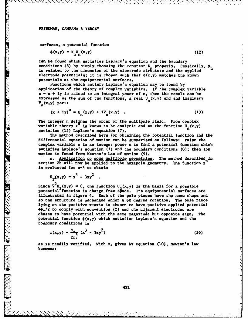
-. *-.*- ---. -t -7-7-7-
FRIEDMAN, CAMPANA & YERGEY
surfaces, a potential function
¢(x,y) - K U (x,y) (12)n n
can be found which satisfies Laplace's equation and the boundaryconditions (8) by simply choosing the constant K properly. Physically, Kis related to the dimension of the electrode structure and the appliedelectrode potentials; it is chosen such that O(x,y) matches the knownpotentials at the equipotential surfaces.
Functions which satisfy Laplace's equation may be found byapplication of the theory of complex variables. If the complex variablez - x + iy is raised to an integral power of n, then the result can beexpressed as the sum of two functions, a real Un (x,y) and and imaginaryV (x,y) part:n
(x + iy)n _ U (x,y) + xiV(x,y) (13)n n
The integer n defAnes the order of the multipole field. From complexvariable theory z is known to be analytic and so the function U n(x,y)satisfies (15) Laplace's equation (7).
The method described here for obtaining the potential function and thedifferential equation of motion can be summarised as follows: raise thecomplex variable z to an integer power n to find a potential function whichsatisfies Laplace's equation (7) and the boundary conditions (8); then ionmotion is found from Newton's Law of motion (9).
c. Application to some multipole geometries. The method described ninsection 2b will now be applied to the hexapole geometry. The function zis evaluated for n-3 to obtain
.- 3 2U x,y) -x - 3xy
Since V2U3 (x,y) - 0, the function U (x,y) is the basis for a possiblepotential function in charge free space. Its equipotential surfaces areillustrated in figure 4. Each of the pole pieces have the same shape andso the structure is unchanged under a 60 degree rotation. The pole piecelying on the positive x-axis is chosen to have positive applied potential+4./2 to comply with convention (2) and the adjacent electrodes arechosen to have potential with the same magnitude but opposite sign. Thepotential function O(x,y) which satisfies Laplace's equation and theboundary conditions is
*(xy) (X - 3xy2) (16)2r.
as is readily verified. With *o given by equation (10), Newton's lawbecomes:
421
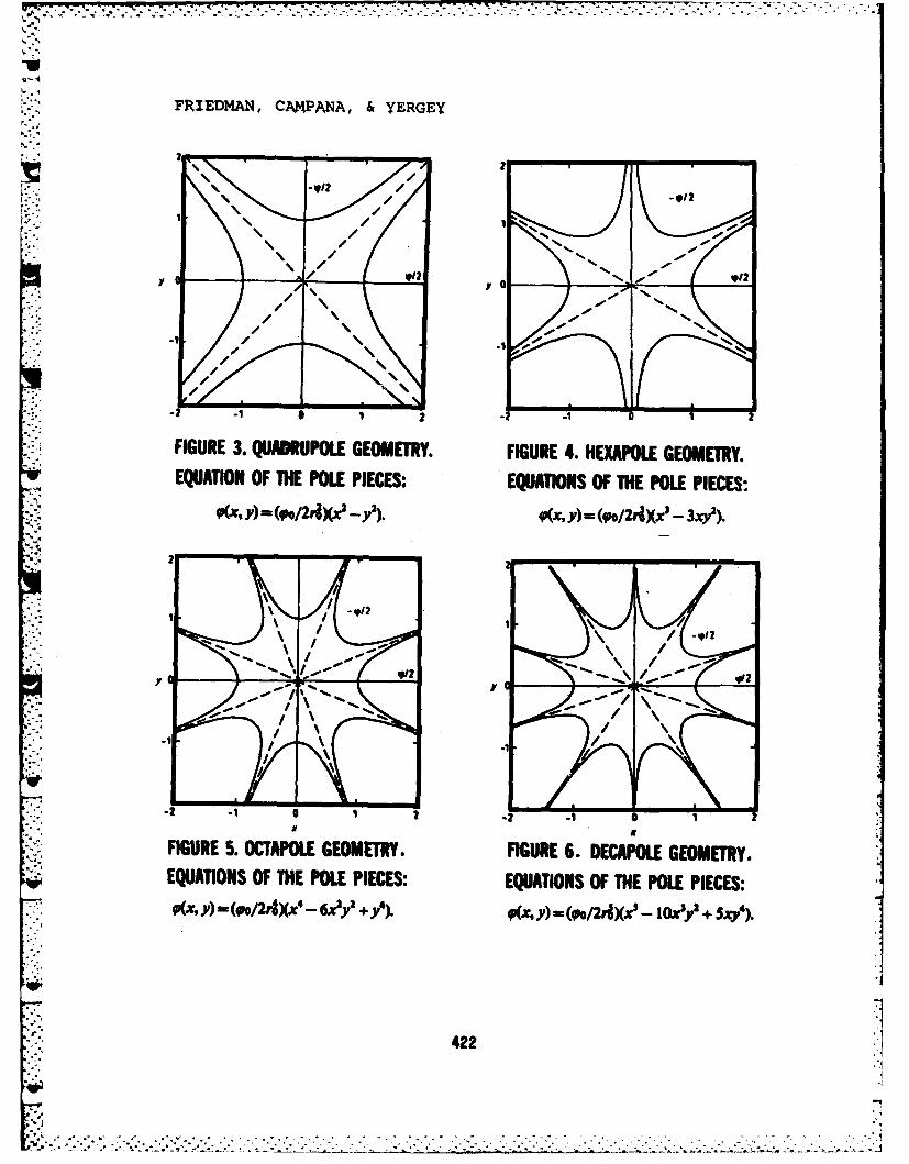
FRIEDMAN, CAMPANA, &YERGEY
t#1
'00,
FIGURE 3. QUADRUPOLE GEOMETRY. FIGURE 4. HEXAPOLE GEOMETRY.EQUATION OF THE POLE PIECES: EQUATIONS OF THE POLE PIECES:
q(x. y) = (v./2AiX'y). qi~x, y) =(.p/2AX'- 3m9).
52 2
FIGURE 5. OCTAPOLE GEOMETRY. FIGURE 6. DECAPOLE GEOMETRY.EQUATIONS OF THE POLE PIECES: EQUATIONS OF THE POLE PIECES:4Kx, y) (Vo/2r8Xx' - 6x2 y') V(x, y) =(vo/2riXx' - I Wy + Sxy4).
422
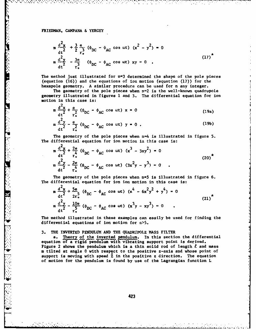
FRIEDMAN, CAMPANA & YERGEY
2m A + 3 (D C-Ccos Wt) (x 2 - 2 0
2 T23 DCACdt r0 ,
(17)_ 3e (CDC-Acos t) xy 0dt ro
The method just illustrated for n-3 determined the shape of the pole pieces(equation (16)) and the equations of ion motion (equation (17)) for thehexapole geometry. A similar procedure can be used for n any integer.
The geometry of the pole pieces when n=2 is the well-known quadrupolegeometry illustrated in figures 1 and 3. The differential equation for ionmotion in this case is:
d2xm --+!2 (DC -AC cos t) x (19a)
dt r.
m 2 - DC AC Cos (t) y = 0 (19b)
+ dt2 r,
The geometry of the pole pieces when n=4 is illustrated in figure 5.The differential equation for ion motion in this case is:
dx 2e 3 y2m--+- (DC - ACcos Wt) (x3 2
dt r0 (20)*
m 4Z e 2 3m 2 (0DC - AC cos wt) (3xy - y 0
dt r.
The geometry of the pole pieces when n=5 is illustrated in figure 6.
The differential equation for ion ion motion in this case is:d2x 5e 4 2
m- +-- (DC 2eC Cos Wt) (x - 6x2y 2 + y) 02 5 -DC ACc,
dt 2r
+__ (21)
y l5 (0D - ACcos Wt) (x y - xy3 0 .dt" d 2 ro DC A
The method illustrated in these examples can easily be used for finding the
differential equations of ion motion for n>5.
3. THE INVERTED PENDULUM AND THE QUADRUPOLE MASS FILTERa. Theory of the inverted pendulum. In this section the differential
equation of a rigid pendulum with vibrating support point is derived.Figure 2 shows the pendulum which is a thin solid rod of length t and massm tilted at angle e with respect to the positive z-axis and whose point ofsupport is moving with speed Z in the positive z direction. The equationof motion for the pendulum is found by use of the Lagrangian function L
423
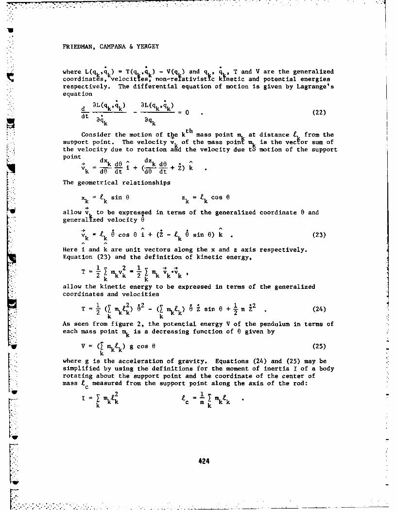
71 5. FRIEDMAN, CAMPANA & YERGEY
where L(q k,qk = T(q ,qi) - V(q ) and q1, q T and V are the generalizedcoordinates, velocitiesk non-reiativisttc ktnetic and potential energiesrespectively. The differential equation of motion is given by Lagrange'sequation
-:' d3L(qk'qk 9L(qk'qk
-0 . (22)dt q;k qk
thConsider the motion of the k mass point m1 at distance e from the
support point. The velocity vk of the mass point mk is the vec or sum ofthe velocity due to rotation and the velocity due to motion of the supportpoint dx dzk
-"k dO k dOvk dO TE i + (--+ Z) k
The geometrical relationships
: -. 'x k = s i n 0 z k = k C o s 0Xk k k kZ cs
allow v. to be expressed in terms of the generalized coordinate e andgeneralized velocity e
V k = t k 0 cos 0 i + (Z - k sin 0) k . (23)
Here i and k are unit vectors along the x and z axis respectively.Equation (23) and the definition of kinetic energy,
T 2 v nkvk = 2 X VkVkk k
allow the kinetic energy to be expressed in terms of the generalized
coordinates and velocities
T =*2 (24)T m ) 2- ( mkZk) 2 sine:m
k 2As seen from figure 2, the potential energy V of the pendulum in terms ofeach mass point mk is a decreasing function of e given by
V = (m iktk) g cos e (25)k
where g is the acceleration of gravity. Equations (24) and (25) may besimplified by using the definitions for the moment of inertia I of a bodyrotating about the support point and the coordinate of the center of
mass t measured from the support point along the axis of the rod:c
mktketc -M! I .I2k k
L 424K?.
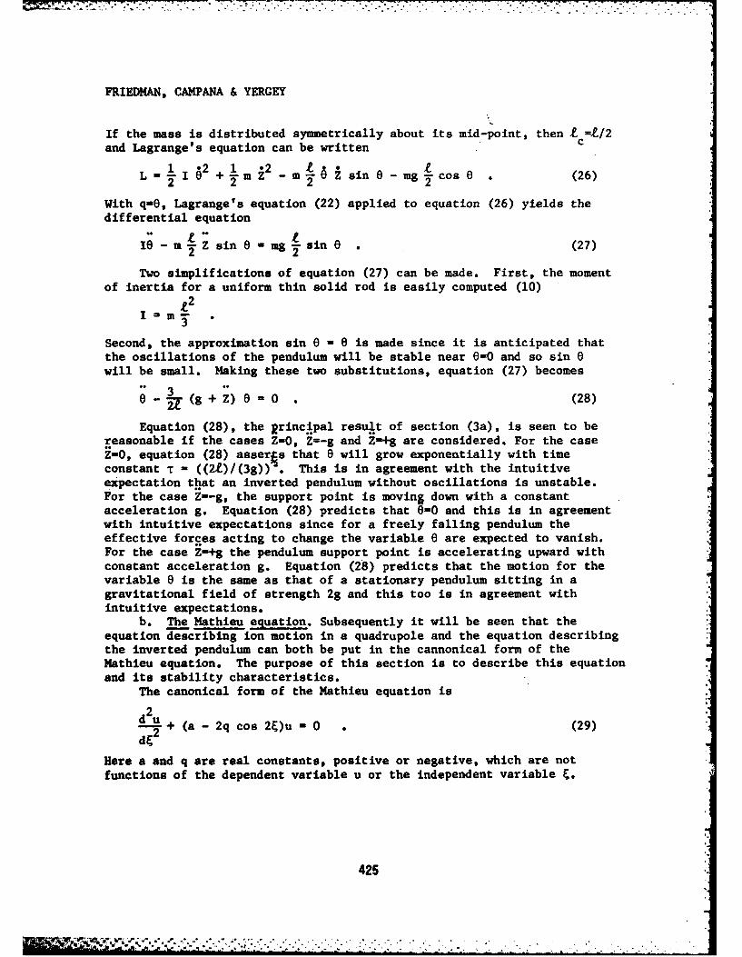
.7.7
FRIEDMAN, CAMPANA & YERGEY
If the mass is distributed symmetrically about its mid-point, then t =/2and Lagrange's equation can be written C
L - 11 62 +.1 m 2 _ m t 6 i sin 0 - mg cos (26)2 +m 2 2--
With q-0, Lagrange's equation (22) applied to equation (26) yields thedifferential equation
0- m -Zsin m - sin 0 (27)
Two simplifications of equation (27) can be made. First, the momentof inertia for a uniform thin solid rod is easily computed (10)
£2
Second, the approximation sin 0 - 0 is made since it is anticipated thatthe oscillations of the pendulum will be stable near 0-0 and so sin 0will be small. Making these two substitutions, equation (27) becomes
- (g+z)8-0 . (28)
Equation (28), the Rrincipal result of section (3a), is seen to bereasonable if the cases Z-0, Z=-g and Z-+g are considered. For the caseZ-0, equation (28) asserts that 8 will grow exponentially with timeconstant T - ((2t)/(3g)) . This is in agreement with the intuitiveexpectation that an inverted pendulum without oscillations is unstable.For the case Z--g, the support point is moving down with a constantacceleration g. Equation (28) predicts that 0-0 and this is in agreementwith intuitive expectations since for a freely falling pendulum theeffective forces acting to change the variable 0 are expected to vanish.For the case Z-+g the pendulum support point is accelerating upward withconstant acceleration g. Equation (28) predicts that the motion for thevariable 0 is the same as that of a stationary pendulum sitting in agravitational field of strength 2g and this too is in agreement withintuitive expectations.
b. The Mathieu equation. Subsequently it will be seen that theequation describing ion motion in a quadrupole and the equation describingthe inverted pendulum can both be put in the cannonical form of theMathieu equation. The purpose of this section is to describe this equationand its stability characteristics.
The canonical form of the Mathieu equation is
2d - + (a - 2q cos 2&)u -0 (29)d&
2
Here a and q are real constants, positive or negative, which are notfunctions of the dependent variable u or the independent variable F.
425
lP ' w '
' S. . . . . . ." """'" """ " '. . . . . . " . . . ... ." 4 I
-g
FRIEDMAN, CAMPANA & YERGEY7:7.
Figure 7. The a-q stability diagram.Equation (29) defines the parameters a andq which appear in the Mathieu equation.For a and q values which fall in theshaded area the value of u in equation 29
1 5 1 q 15 remains bounded as E increases independ-ent of the initial conditions. Othervalues of a and q result in unboundedsolutions.
Although the factor -2 multiplying q and the 2 in the argument of thecosine function might look strange, this is the standard for of this 23differential equation whose properties have been extensively studied. '
The solution of equation (29) will be a function of the form
u = u(E; a,q,uo,Uo) • (30)
Equation (30) expresses mathematically the observation that the functionV, u depends on the independent variable E, on the parameters a and q, on the
initial value of u denoted by u., and on the initial value of du/dEdenoted by it. The function (30).evaluated for a particular value of aand q is a function of E, u. and u.. The result of detailed mathematicalanalysis (22) is that, depending on the values of the parameters a and q,the function u becomes unbounded or remains bounded as E increases andthat these values of a and q are independent of the initial conditionsu. and Uo. Figure 7 shows a portion of a stability diagram in a-q space.The shaded area results in "stable" trajectories by which it is meant thatu remains within finite bounds as E increases independent of initialconditions.
c. Analogy between inverted pendulum and quadrupole mass filter. Inthis section it is shown that both the inverted pendulum and the QMF canbe expressed in the cannonical form of the Mathieu equation and theanalogs will be identified.
In equation (28) 2 is the acceleration of the support point. If thesupport point is driven sinusoidally with frequency w, then the origin oftime can be chosen so that Z b cos wt. In that case, equation (28)becomes
d2 6 3 2--- 2(g -bw cos wt) 0 (31)dt
Define four dimensionless parameters
(a) u 0 (b) a
tw2+ + ow t 3 b ( 3 2 ) + : ,
(c) E (d) q=.- (32)
42.
• ., ,+' ;.+2".,,.. . .. .. . . . . .. . . . . . . . .. . . . .
FRIEDMAN, CAMPANA & YERGEY
and use these to replace the variables 8 and t in equation (31) to get thecannonical form of the Mathieu equation (29).
Note that equations (19a) and (19b) are essentially the same asidefrom a change in sign and so without loss of generality only equation(19b) is considered in drawing the analogy with the inverted pendulum.Define four dimensionless parameters
4eDC(a) u - y (b) a 2e2
r," (33)2eoAC
(c) - (d) q A C~22
and use these to replace y and t in equation (19b) to get the cannonicalform of the Mathieu equation (29).
From equations (32) and (33) the analogous quantities can be ident-ified. Multiplying numerator and denominator of equation (32b) by m, themass of the pendulum, and comparing equations (32b) and (33b), aside fromsome unimportant numerical factors, the quantity mg of the pendulum isanalogous to (eoDC)/r. of the QMF; at of the pendulum is analogous to mr,of the QMF and w of the pendulum is analogous to w of the QMV.Multiplying numerator and denominator of equation (32d) by mW2 andcomparing equations (32d) and (33d); aside from some unimportantnumerical factors, the quantity bmwi of the pendulum is analogous to(eaC)/r. of the QMF; m of the pendulum is analogous to mro of the QMFand w of the pendulum is analogous to ,wi of the QMF. In these analogies,all the quantities associated with the pendulum have the same physicaldimensions as the corresponding quantities associated with the QMF. Also,the RF source of the QMF end the oscillating source for the support pointin the inverted pendulum perform analogous functions of producing astability mechanisim for each system. The destabilizing terms of eachsystem are g, the acceleration of gravity for the inverted pendulum,and , the applied DC voltage of the QMF. The quantities which counterthese Destabilizing terms are bW2, the acceleration amplitude for thesupport point of the inverted pendulum and *AC' the RF amplitude ofthe QMF.
4. CONCLUSIONS.Explicit differential equations in closed form have been found for
pole piece geometries which are generalizations of those used in theQMF, For arbitrarily shaped pole pieces, the solution of Laplace'sequation cannot be written in closed form and, thus in general the iondifferential equations of motion cannot be written in closed form. Thegeometries shown in figures 4, 5 and 6 are analytically useful indetermining if other geometries might yield mass filters with improvedresolution/transmission characteristics. Computer simulation of ionmotion in these geometries is a subject for future research.
I . .
-
427
_ -.
FRIEDMAN, CAMPANA & YERGEY
Although not reported in this paper, an inverted pendulum has beenbuilt (10) and it has been useful in emphasizing to students the non-intuitive nature of the mass filtering action that takes place in a QMF.In reference (10), it is shown conceptually that the inverted pendulumcan be used to experimentally measure the boundaries between the stableand unstable regions in the a-q stability diagram. As a result, theinverted pendulum aids in understanding these diagrams which are crucialto understanding the operation of a QMF.
The principal new results of our research are: 1) new derivations ofthe equations which describe ion motion in a QMF, 2) the equations of polepieces for hexapole, octupole and decapole geometries illustrated infigures 4, 5 and 6, 3) closed form differential equations of ion motion inthese geometries (equations (17), (20) and (21)) and 4) the realizationthat the inverted pendulum is a mechanical analog of the QMF.
Today the quadrupole mass analyser is the most widely used massanalyser for low resolution applications. Typically, mass filters areused in laboratory environments where simplicity, compactness, economy,absence of magnetic fields, and/or the capability of fast scan rates(especially for chromatographic combinations) are important (1). Thus,an improvement in resolution/transmission qualities of electric RF massfilters would enable this widely used mass spectrometer to take a largerrole in analytical laboratories and in basic research. Other designconsiderations besides resolution/transmission characteristics areimportant. If mass filters could be made which are smaller, more rugged,less susceptible to vibration with reduced power requirements, and moreeasily maintained, there might be greater application outside thelaboratory. Possible applications include: surveying for naturalresources, pin-pointing sources of industrial pollutants, and thedetection of hazardous materials such as chemical agents and explosives.Eventually our work may be applied to the solution of these problems.
REFERENCES
1. J. E. Campana, Elementary Theory of the Quadrupole Mass Filter,
Int. J. Mass Spectrom. Ion Pha33, 101 (1980).2. P. H. Dawson (Ed), Quadrupole Mass Spectrometry and its Applications, _.-4
Elsevier, Amsterdam (1976).* 3. H. C. Corben and P. Stehle, Classical Mechanics, John Wiley and Sons,
New York (1960).4. L. D. Landau and E. M. Lifshitz, Mechanics, Pergamon Press, London
(1960).5. P. L. Kapitza, in D. ter Haar (Ed), Collected Papers of P. L. Kapitza,
Pergamon Press, London (1965) pp 714, 726.6. H. P. Kalmus, The Inverted Pendulum, Am. J. ys. 3.18, 874 (1970).
428
* - .*. . . .. . . . .. -.. .. . . . .
. . . . . . . . . . . .. . . . . . . .
. . . ..r - r rr.-.-r-.-- - - . . . .
FRIEDMAN, CAMPANA & YERGEY
7. R. Mitchell, Stability of the Inverted Pendulum Subjected to AlmostPeriodic and Stochastic Base Motion - An Application to the Method ofAveraging, Int. J. Non-Linear Mech. 7, 101 (1974).
8. M. S. Howe, The Mean Square Stability of an Inverted Pendulum Subjectto Random Parametric Excitation, J. Sound Vib. 32, 407 (1974).
9. E. C. Yorke, Square-Wave Model for a Pendulum With OscillatingSuspension, AE. J. Phys. 46 , 285 (1978).
10. M. H. Friedman, J. E. Campana, L. Kelner, E. H. Seeliger and A. L.Yergey, The Inverted Pendulum: A Mechanical Analog of the QuadrupoleMass Filter, Am. J. Phys., in press.
11. M. H. Friedman, A. L. Yergey and J. E. Campana, Fundamentals of IonMotion in Electric Radio Frequency Fields, J. Phys. E: Sci. Instr. 15,53 (1982).
12. E. M. Pugh and E. W. Pugh, Principles of Electricity and Magnetislim,Addison-Wesley, Reading, MA (1960).
13. S. Ramo, J. R. Whinnery, T. van Duzer, Fields and Waves in Cowaun-ication Electronics, John Wiley and Sons, New York (1965).
14. J. D. Jackson, Classical Electrodynamics, John Wiley, New York (1962).15. R. V. Churchill, Complex Variables and Applications, McGraw-Hill,
New York (1941).16. R. V. Churchill, Fourier Series and Boundary Value Problems,
McGraw-Hill, (1963).17. K. J. Binns and P. J. Lawrenson, Analysis and Computation of Electric
and Magnetic Field Problems, Macmillan, New York (1963).18. M. G. Salvadori and M. L. Baron, Numerical Methods in Engineering,
Prentice Half, Englewood Cliffs, N.J. (1964).19. V. Vemuri and W. J. Karplus, Digital Computer Treatment of Partial
Differential Equations- Prentice Hall, Englewood Cliffs, N.J. (1981).20. W. Paul and H. Steinwendel, A New Mass Spectrometer Without a
Magnetic Field, Z. Naturforsch 8a, 448 (1953).21. W. Paul. H. P. Reinhard, U. von Zahn, The Electric Mass Filter as Mass
Spectrometer and Isotope Separator, Z. Phys. 152, 143 (1958).22. N. W. McLachlan, Theory and Application of Mathieu Functions, Oxford
University Press, London (1947).23. M. Abramowitz and L. A. Stegun (Ed), Handbook of Mathematical
Functions With Formulas, Graphs and Mathematical Tables, NationalBureau of Standards, Applied Mathematics Series 55 (1964).
LI 429
K.
GAUSS
A NEW TYPE OF ER WAVE ABSORBING COATING
ARTHUR GAUSS, Jr., Ph.D.BALLISTIC RESEARCH LABORATORY, ARRADCOMABERDEEN PROVING GROUND, HD 21005
Introduction
Research on radar anti-reflection coatings has been actively pursuedboth theoretically and experimentally since World War II. Interference,(1,2) dielectric (3), and magnetic-dielectric (4,5) absorptive coatingshave been tried.
Recently a new type of radar absorbing chaff (RAC) has been sug-gested (6). Calculations done at BIL indicate that by compacting the RACfilaments a new type of radar absorbing coating (called RACO) may be pos-sible. The filaments would be fixed in a solid binder having near unitydielectric constant. The primary mechanism for attenuation of the incidentradiation by a RAC cloud or RACO layer is by resistive dissipation in therelatively long, thin chaff filaments. The tiny RAC-RACO filaments havelength to diameter ratios on the order of one thousand with diameters ofabout 500A. Filament separations in a RACO are about one-half to one-thirdof a filament length thus requiring the inclusion of dipole and perhapshigher order interactions. Each filament can be modeled simply as a series
..resistive-capacitive circuit, single filament theory will be discussed inSection II.
RACOes are divided into two classes, regular and random. RegularRACO's are regular arrays of parallel RAC filaments. Random RACO's arerandom collections of randomly oriented filaments. The resistive-capacitive nature of each filament enables us to express the dielectricconstant of a RACO (regular or random) in terms of a simple relaxationmechanism which is mathematically equivalent to the Debye theory from solidstate physics (7). The Debye formalism is readily adaptable to include di-pole interactions. Regular RACO theory is analyzed in Section III, and re-flectance data are calculated for a regular RACO over a metal substrate.In addition to the Debye theory the Onsager dielectric constant theory (8)
431
.. % . , . .
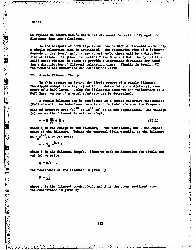
GAUSS
is applied to random RACO's which are discussed in Section IV; again re-flectance data are calculated.
In the analyses of both regular and random RACO's discussed above only.. , a single relaxation tie Is considered. The relaxation time of a filament
depends on its length and, in any actual RACO, there will be a distribu-tion of filament lengths. In Section V the Cole and Cole theory (9) fromsolid state physics is shown to provide a convenient formalism for handl-ing a distribution of filament relaxation tues. Finally in Section VIthe results are summarized and conclusions drawn.
II. Single Filament Theory
In this section we derive the dipole moment of a single filament.The dipole moment Is a key ingredient in determining the dielectric con-stant of a RACO laver. Using the dielectric constant the reflectance of aRACO layer on top of a metal substrate can be determined.
A single filament can be considered as a series resistive-capacitance(R-C) circuit. An inductance term is not included since at the frequen-
10 11cies of interest here (10 to 10 Ha) it Is not significant. The voltage(v) across the filament is written simply
dt (11.1)
where q is the charge on the filament, R the resistance, and C the capaci-tance of the filament. Taking the external field parallel to the filament
n.as I e1t.1 we can write0v = E 0 ea I.
where Z is the filament length. Since we wish to determine the dipole mom-ant (p) we write
q p/1
The resistance of the filament is gIvan by
R
whera o is the filament conductivity and A is the cross sectional area.The capacitance is given by
432
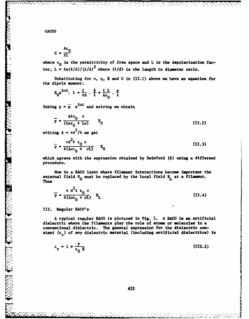
". GAUSS
C Ae0
IL
where e is the permittivity of free space and L is the depolarization fac-
tor, L - tn(X/d)/(t/d)2 where (t/d) is the length to diameter ratio.
Substituting for v, q, R and C in (II.1) above we have an equation forthe dipole moment:
i t +-0 aA 9 t
Taking p - p e and solving we obtain
Ale o- __ M Uwe + E (O).2)
00
writing A - rd 2/4 we get
2
ird,0-E (11.3)= 4(iwe + 0L) 0
which agrees with the expression obtained by Swinford (6) using a differentprocedure.
Now in a RACO layer where filament interactions become important theexternal field E0 must be replaced by the local field EL at a filament.Thus
4 (iwe + L (1.4)
1II. Regular RACO's
A typical regular RACO is pictured in Fig. 1. A RACO is an artificialdielectric where the filaments play the role of atoms or molecules in aconventional dielectric. The general expression for the dielectric con-stant (er) of any dielectric material (including artificial dielectrics) is
r
.....r + C.
,....,433
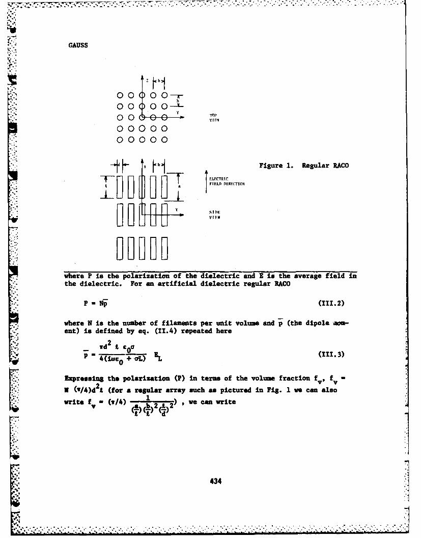
.. GAUSS
00 00 -r00 00-
0000000000
A'.. xb Figure 1. Regular RACO
E.LECTRICFIED . I. RFIION
Y D
where P is the polarization of the dielectric and E is the average field inthe dielectric. For an artificial dielectric regular RACO
P - Np (111.2)
where N is the number of filaments per unit volume and p (the dipole ma-ent) is defined by eq. (11.4) repeated here
.rd 2 + &L F (111.3)
.0 + OL)
Expressing the polarization (P) in term of the volume fraction fv, fvv
i (/4)d 2I (for a regular array such as pictured in Fig. 1 we can also
write fI 0/4) w a b l ve can write
434
GAUSS
e0 fvP+ L) E (111.4)
It can be shown that the average field E in the dielectric is related tothe local field EL by the following (10,11)
E P (111.5):":.. E- EL -A €---
where A is the dipole interaction factor and depends on the array geometryof the RACO. Substituting (111.5) into (111.1) and using (111.4) we ob-tain
Cr -I+ 1 1 (111.6)r 1
where T is the single fIlmment relaxation time given by the product RC (seeSection II) - C0/aL, and x = fv/L.
The above, (111.6), has the Debye form of the dielectric constant fromsolid state physics. The Debys form is (7)
C r -Cr = + r r, (111.7)
which matches (111.6) with the identifications
era,
xLr0 r-- -Ax
and
T T
For the purposes of reflectance calculations two versions of the di-electric constant expression will be used. One version is identical to
435
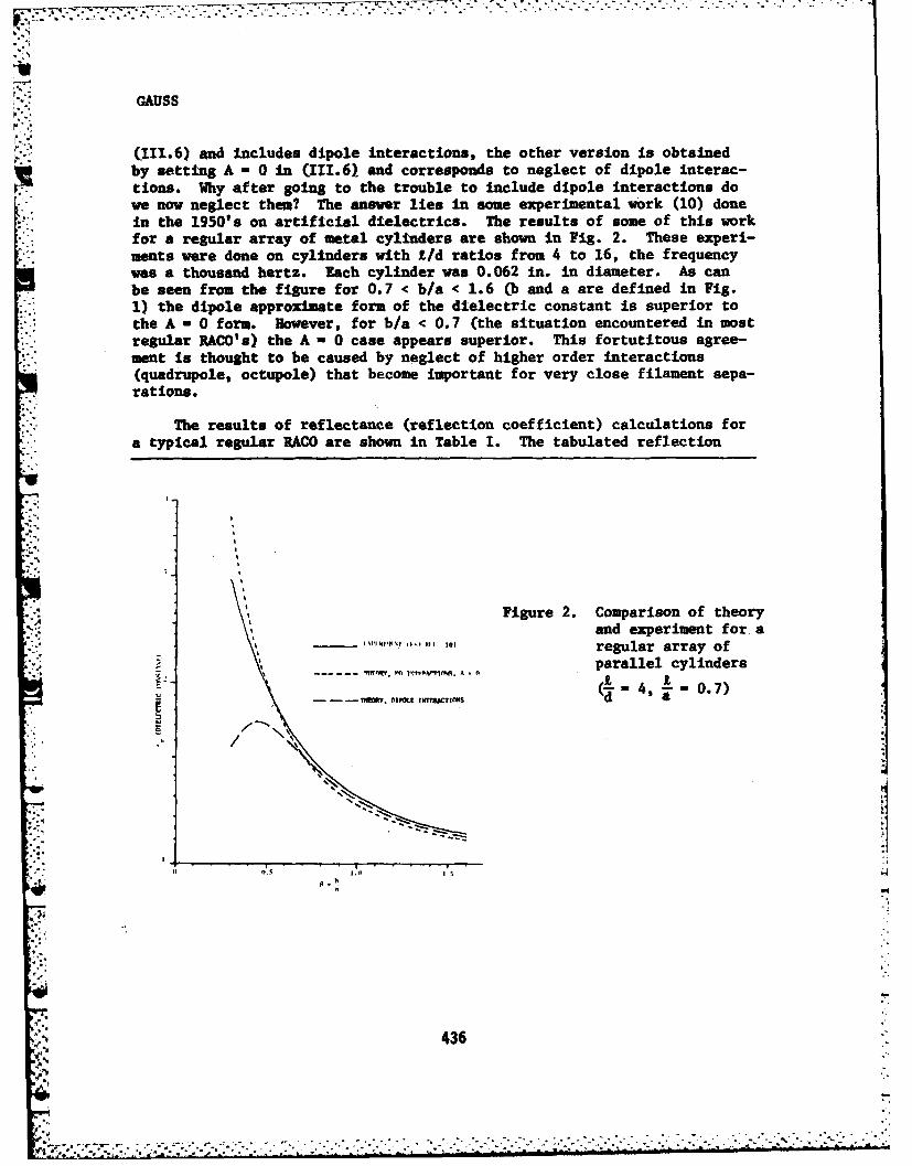
GAUSS
(111.6) and Includes dipole interactions, the other version is obtainedby setting A - 0 in (111.6) and corresponds to neglect of dipole interac-tions. Why after going to the trouble to include dipole interactions dowe now neglect them? The answer lies in some experimental work (10) donein the 1950's on artificial dielectrics. The results of some of this work
for a regular array of metal cylinders are shown in Fig. 2. These experi-ments were done on cylinders with 1/d ratios from 4 to 16, the frequencywas a thousand hertz. Each cylinder was 0.062 in. in diameter. As canbe seen from the figure for 0.7 < b/a < 1.6 (b and a are defined in Fig.1) the dipole approximate form of the dielectric constant is superior tothe A - 0 form. However, for b/a < 0.7 (the situation encountered in mostregular RACO's) the A - 0 case appears superior. This fortutitous agree-ment is thought to be caused by neglect of higher order interactions(quadrupole, octupole) that become important for very close filament sepa-rations.
The results of reflectance (reflection coefficient) calculations for
a typical regular RACO are shown in Table I. The tabulated reflection
Figure 2. Comparison of theoryand experiment for a
I"Iik1I NI F0 1 regular array of
" N).."'.... A A parallel cylinders
4 4, - 0.7)
IM I P INTJ TM
,:. ., . . .. . . .
klIN,
-oi!436
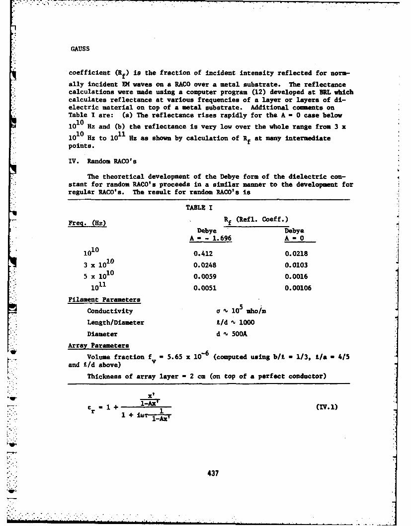
"--
GAUSS
coefficient (Rf) is the fraction of incident intensity reflected for norm-
ally incident Dl waves on a RACO over a metal substrate. The reflectancecalculations were made using a computer program (12) developed at BRL whichcalculates reflectance at various frequencies of a layer or layers of di-electric material on top of a metal substrate. Additional comments onTable I are: (a) The reflectance rises rapidly for the A - 0 case below
1010 Hz and (b) the reflectance is very low over the whole range from 3 x
110 Hz to 10 Hz as shown by calculation of Rf at many intermediatepoints.
IV. Random RACO's
The theoretical development of the Debye form of the dielectric con-stant for random RACO's proceeds in a similar manner to the development forregular RACO's. The result for random RACO's is
TABLE I
Freq. (Hz) Rf (Refl. Coeff.)
Debye DebyeA - - 1.696 A - 010I
1010 0.412 0.0218 I3 x 1010 0.0248 0.0103
5 x 10¹⁰ 0.0059 0.0016
1011 0. 0051 0.00106
Filament Parameters
Conductivity a 10 5 mho/m
Length/Diameter I/d " 1000
Diameter d " 500A
Array Parameters
Volume fraction f - 5.65 x 10⁻⁶ (computed using b/t - 1/3, I/a - 4/5and L/d above) v
Thickness of array layer - 2 cm (on top of a perfect conductor)
1- + ---- (V.1)r1
,'- -'437
-u
GAUSS
where x = f /3L (the factor of 3 arises from the random orientation of theV
dipoles), T - e0 /aL is the single filament relaxation time and A is the di-
pole interaction factor.
For the reflectance calculations we take two values of A in eq. (IV.l);namely A - 0 and A - 1/3. The first corresponds to the neglect of the di-pole interactions between filaments whereas the second can be shown to re-present a reasonable approximation for a random collection of aligned di-poles. It may be recalled that in most polar substances (and in randomRACO's) the dipoles are not aligned and A - 1/3 is known to be a poor ap-proximation (8). On the other hand some authors (13) believe A - 0 is thecorrect approximation for polar materials.
Another theoretical expression for the dielectric constant may be de-rived for subsequent use in reflectance calculations for random RACO's.This expression is similar to that used by Onsager (8) for random collec-tions of polar molecules. In this theory a typical RACO filament repre-sented by a point dipole is assumed to lie in a real spherical cavity inthe artificial dielectric. The local electric field in the cavity isgiven by (14)
3e
rEL 2 + F' (iv.2)r
The dipoles are randomly oriented so the average dipole moment parallel tothe field is p' - p/3. Hence using eq. (I.14) we obtain
Ale0 aP 3(w + oL) L (V.3)
Hence the polarization may be written as
P 'N (IV.4)
*: Substituting (IV.4), (IV.3) and (IV.2) into the basic equation
and 6 E - E + P where er 0r C0
and defining
oof
10 vK 3(iwc0 + al.
'.,
438
---------------..... . . ... .........
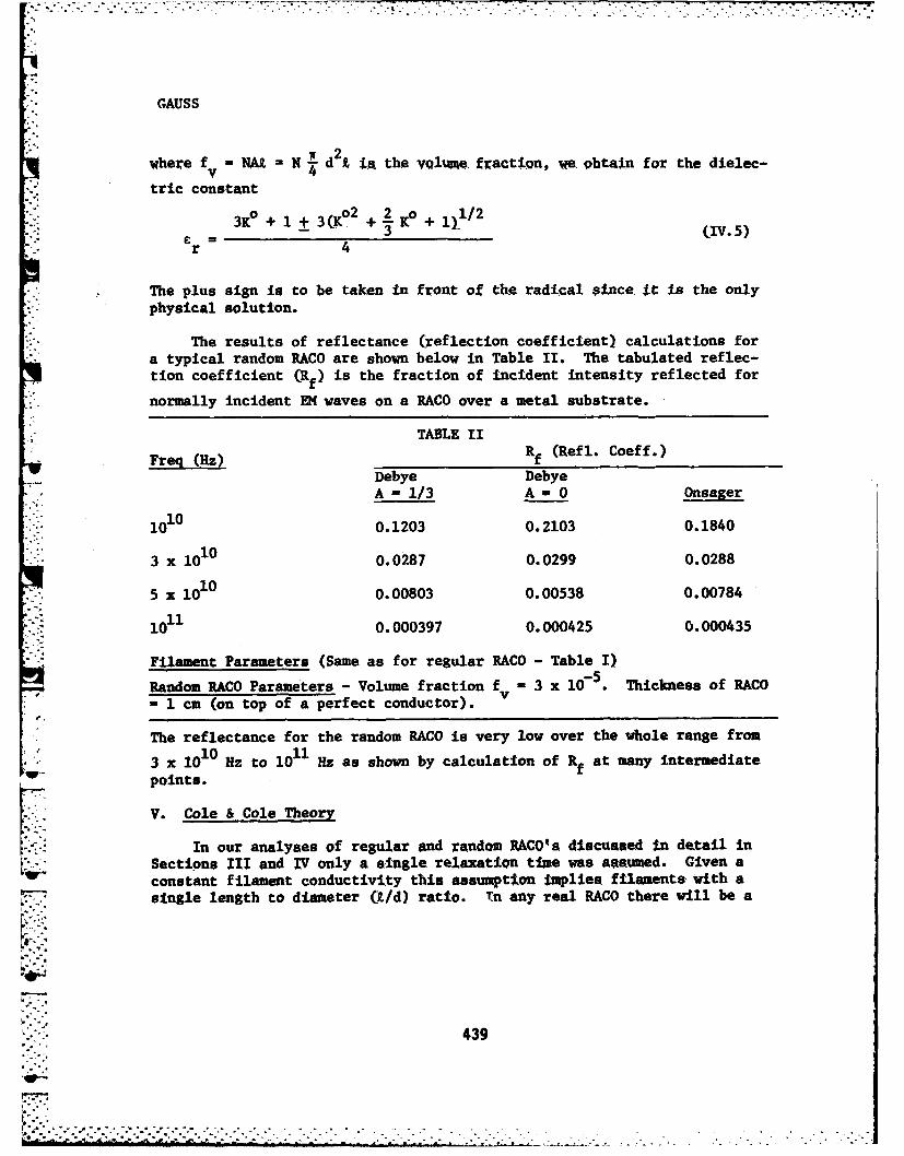
-. ° - . - - .- .- .-- .- -- • rr'- ."rrr ,- -t . . , - . . , • . = __ J
GAUSS
where fv NAd N d 2 IaL the vQlume. fraction, we obtain for the dielec-
tric constant
3o2 o + 11/23e + i + 3 K+1
3 (IV.5)r 4
The plus sign is to be taken in front of the radical since. it Is the onlyphysical solution.
The results of reflectance (reflection coefficient) calculations fora typical random RACO are shown below in Table II. The tabulated reflec-tion coefficient (Rf) is the fraction of incident intensity reflected for
*normally incident EM waves on a RACO over a metal substrate.
TABLE II
Freg (Hz) Rf (Refl. Coeff.)
Debye DebyeA - 1/3 A - 0 Onsager
1010 0.1203 0.2103 0.1840
3 x 1 0 0.0287 0.0299 0.0288
5 x 10¹⁰ 0.00803 0.00538 0.00784
1011 0.000397 0.000425 0.000435
Filament Parameters (Same as for regular RACO - Table I)
Random RACO Parameters - Volume fraction f - 3 x 10⁻⁵. Thickness of RACO- 1 cm (on top of a perfect conductor).
v
The reflectance for the random RACO is very low over the whole range from
3 x 10¹⁰ Hz to 10 1 Hz as shown by calculation of Rf at many intermediatepoints.
KV. Cole & Cole Theory
In our analyses of regular and random RACO0a discussed in detail inSections III and IV only a single relaxation time was assumed. Given aconstant filament conductivity this assumption implies filaments with asingle length to diameter (£/d) ratio. Tn any real RACO there will be a
439
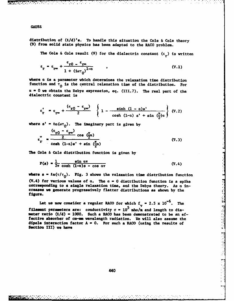
GAUSS
distribution of (L/d)'s. To handle this situation the Cole & Cole theory(9) from solid state physics has been adapted to the RACO problem.
The Cole & Cole result (9) for the dielectric constant (c r) is written
+ C r0- Cra (V.I)Cr r- 1 + (iw-r0)l- v1
where a is a parameter which determines the relaxation time distributionfunction and T0 is the central relaxation time of the distribution. For
a - 0 we obtain the Debye expression, eq. (111.7). The real part of thedielectric constant is
, C + (C ) rO r ) sinh ( - a)s'+r -r (V.2)cosh (1-) s' + sin ()a
where s' - Tn( T0 ). The imaginary part is given by
(C 0 - cr -)r 2' cos
C - 2 (V.3)cosh (l-a)s' + sin (a)
The Cole & Cole distribution function is given by
F(s) - sinai (V.4)2w cosh (l-a)s - cos awr
where s l Ln(T/T 0). Fig. 3 shows the relaxation time distribution function
(V.4) for various values of a. The a - 0 distribution function is a spikecorresponding to a single relaxation time, and the Debye theory. As a in-creases we generate progressively flatter distributions as shown by thefigure.
Let us now consider a regular RACO for which f - 2.5 x 10⁶. The
filament pariseters are: conductivity a - 10 mho/m and length to dia-meter ratio (/d) - 1000. Such a RACO has been demonstrated to be an ef-fective absorber of cm-urn wavelength radiation. We will also assume thedipole interaction factor A - 0. For such a RACO (using the results ofSection I1) we have
440
.,..-... -. *.- . . .. . . . . . . . . . .
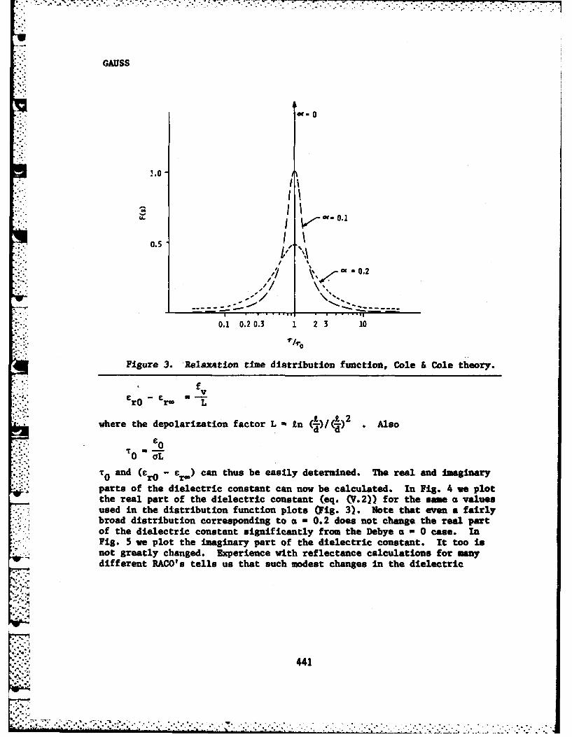
GAUSS
0
.o.0
0.5>!:-, ,\
,: , - 0.2
0.1 0.2 0.3 1 2 3 10o. ,O
Figure 3. Relaxation time distribution function, Cole & Cole theory.
f
rO r- Lwhere the depolarization factor L I Ln / . Also
T F0m~t--
-
,.:::., ' 0 UL'
, and (c - cr) can thus be easily determined. The real and Imaginary0 rO er
parts of the dielectric constant can now be calculated. In Fig. 4 we plotthe real part of the dielectric constant (eq. (V.2)) for the same a valuesused in the distribution function plots ()Fig. 3). Note that even a fairlybroad distribution corresponding to o - 0.2 does not change the real partof the dielectric constant significantly from the Debye a - 0 case. InFig. 5 we plot the imaginary part of the dielectric constant. It too isnot greatly changed. Experience with reflectance calculations for manydifferent RACO's tells us that such modest changes in the dielectric
S441
.- ,.;.',441
,I::
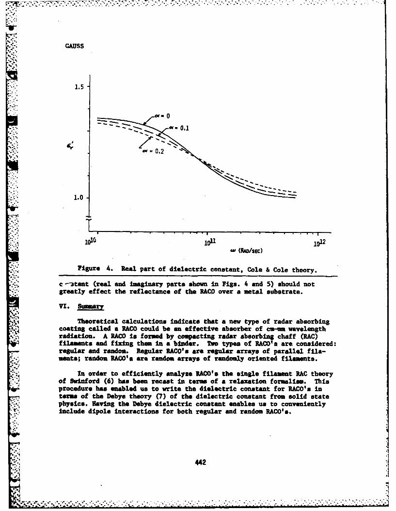
GAUSS
1.5
.9, 4-- o(=0.1
1.0
T.--
106 on 1012w(RAD/sEc)
Figure 4. Real part of dielectric constant, Cole & Cole theory.
c - tant (real and Imaginary parts shown in Figs. 4 and 5) should notgreatly effect the reflectance of the RACO over a metal substrate.
VI. Summary
Theoretical calculations Indicate that a new type of radar absorbingcoating called a RACO could be an effective absorber of cm-ia wavelengthradiation. A RAC is formed by compacting radar absorbing chaff (RAC)filaments and fixing them in a binder. Two types of RACO'a are considered:regular and random. Regular RACO'a are regular arrays of parallel file-
Smea; random RACO's are random arrays of randomly oriented filaments.
In order to efficiently analyze RACO' the single filament RAC theoryof SwInford (6) has been recast in terms of a relaxation formalism. Thisprocedure has enabled us to write the dielectric constant for RACO's interm of the Deby. theory (7) of the dielectric constant from solid statephysics. Having the Debye dielectric constant enables us to convenientlyinclude dipole interactions for both regular and random RACO's.
.•..-.442
~~~s:,~~A ... . . ..... . . . . . . ..
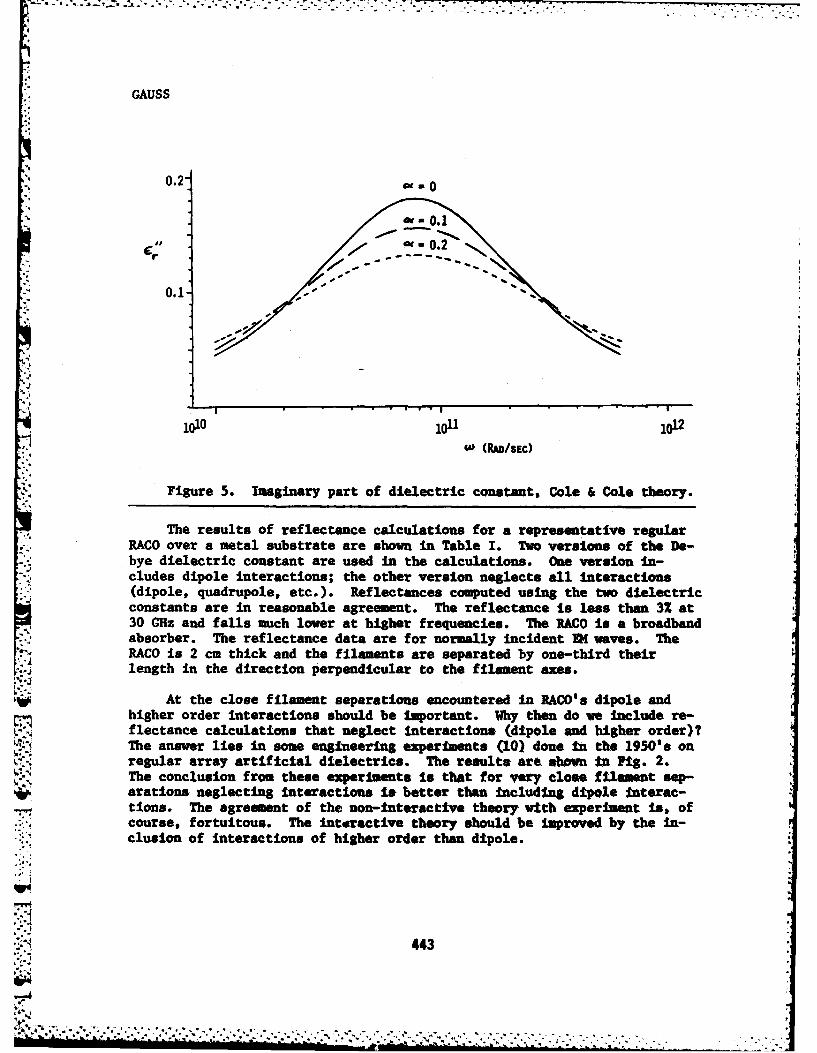
GAUSS
0.2- 0'u
'II
Cr
0.1
1010 1011 1012
l (RA /SEC)
"' Figure 5. Imaginary part of dielectric constant, Cole & Cole theory.
The results of reflectance calculations for a representative regularRACO over a metal substrate are shown in Table I. Two versions of the De-bye dielectric constant are used in the calculations. One version In-cludes dipole interactions; the other version neglects all interactions(dipole, quadrupole, etc.). Reflectances computed using the two dielectricconstants are in reasonable agreement. The reflectance is less than 32 at30 GHz and falls much lower at higher frequencies. The RACO is a broadbandabsorber. The reflectance data are for normally incident DI waves. TheRACO is 2 cm thick and the filaments are separated by one-third theirlength in the direction perpendicular to the filament axes.s.j
At the close filament separations encountered in RACO's dipole andhigher order interactions should be Important. Why then do we include re-
L flectance calculations that neglect nteractions (dipole and higher order)?' The answer lies in some engineering experluents (10C) done n the 1950's on
regular array artificial dielectrics. The result& are shown in Fig. 2.16%. The conclusion from these experiments is that for very close filament sep-
arations neglecting interactions Is better than including dipole interac-tions. The agreement of the non-interactive theory with experiment is, ofcourse, fortuitous. The interactive theory should be improved by the n-clusion of interactions of higher order than dipole.
443
."- .tf il
GAUSS
The results of reflectance calculations for a representative randomRACO over a metal substrate are shown in Table II. Three theoretical ex-pressions for the dielectric constant are used. Reflectances computed us-ing all three expressions are in reasonable agreement. The reflectance isless than 3% at 30 GHz and drops to much lower values at higher frequen-cies. The reflectance data are for normally incident EM waves. The RACOis 1 cm thick and the filament average separation is about one-third thefilament length.
Recent calculations indicate that even thinner RACO's are possible us-*ing a multi-layer coating. Thicknesses of one-half a centimeter or less
appear possible while still giving broadband absorption.
The calculations described above have been done assuming a single re-laxation time. In any real RACO there will be a distribution of filamentlengths and thus a corresponding distribution of relaxation times. To
handle this situation the Cole & Cole theory (9) of solid state physics hasbeen adapted to the RACO problem. This theory demonstrates that n chang-ing from a single relaxation time to a fairly broad distribution of relax-ation times we produce little change in EM wave absorption by RACO's.
While our calculations indicate that RACO's are effective absorbersof cm-un wavelength radar radiation we lack experimental confirmation foractual RACO material. Within the next few months laboratory work on RACO'sshould begin.
References
1. Severin, H., "Non-Reflecting Absorbers for Microwave Radiation," IRETrans. Vol. AP-4, July 1956, pp 385-396.
2. Ryder, J.D., Networks, Lines, and Fields, Prentice-Hall, Inc., Engle-wood Cliffs, NJ, (1960), pp 462-465.
3. Skolnik, M.L., Introduction to Radar Systems, McGraw-Hill Book Com-pany, Inc., New York, (1962), p 565.
4. Thomas, A.S., "Theory of Radar Absorber Material Design QV)," (A.S.Thomas, Inc.1, Techatcal Report AVAL-TR-7G-120, Sep 1970 (SECRET).
5. Mostrom, R.A., "Broadband Radar Absorbers (11," (AVCO Systems Div.,Wilmtngton, MA1, Contract No. DAAR-07-70-C-0194, Aug 1972 (CONFIDN-
. TIAL).
444
GAUSS
6. Svrinford, H.W., "Electromagnetic Behavior of Radar Absorbing Chaff(RAC)," (Naval Weapons Center, China Lake, CA), Technical Note 354-43,June 1975.
7. Von Hippel, A.R., Dielectric Materials and Applications, The MIT Press,Cambridge, MA, (1954).
8. Onsager, L., "Electric Moments of Molecules in Liquids," J. Am. Chem.Soc., (1936), pp 1486-1493.
9. Cole, K.S., Cole, R.H., "Dispersion and Absorption in Dielectrics,"J. Chem. Phys., (1941), pp 341-351.
10. Kharadly, M.M.Z., Jackson, W., "The Properties of Artificial Dielec-trics Comprising Arrays of Conducting Elements," Proc. IEE (London),Vol. 100, Part III, July 1953, pp 199-212.
" 11. Kittel, C., Introduction to Solid State Physics, John Wiley & Sons,Inc., Nev York (1963).
12. Multilayer Normal Incidence Reflectance Program, programm, 1 in Basicfor Tektronix 4051 by A. Gauss, Jr., (to be published).
13. Blakemore, J.S., Solid State Physics, W.B. Saunders Company, Philadel-phia, (1969), p 345.
14. Scott, W.T., The Physics of Electricity and Magnetism, John Wiley &Sons Inc., New York, (1959), pp 137-138.
j.
J 445
NIL,
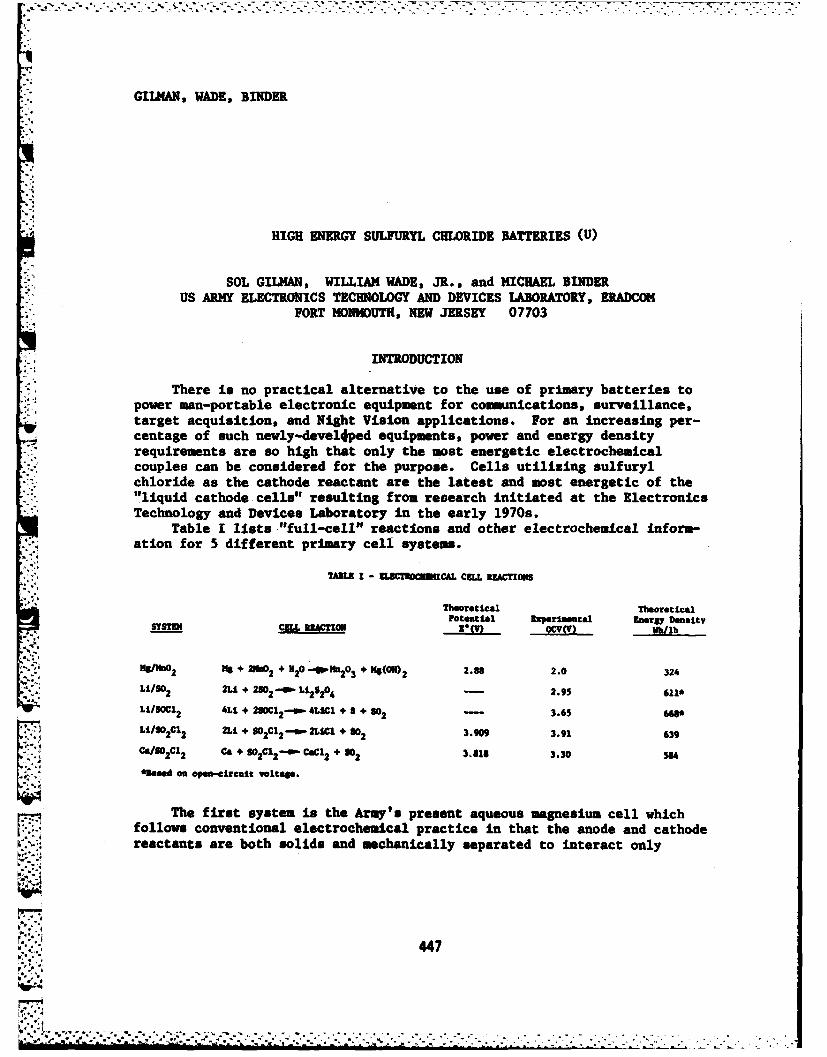
....-- - -• -; -L. c , •. -... --.- -.. . .-.. . . . . . . . . . . . . . . . . . . . . . . . . . . . . . . . . . . . . .' _ , _ . ,
GILMAN, WADE, BINDER
HIGH ENERGY SULmRYL CHLORIDE BATTERIES (U)
SOL GILMAN, WILLIAM WADE, JR., and MICHAEL BINDERUS ARMY ELECTRONICS TECHNOLOGY AND DEVICES LABORATORY, ERADCOM
FORT NONMOUTH, NEW JERSEY 07703
INTRODUCTION
There is no practical alternative to the use of primary batteries topower man-portable electronic equipment for communications, surveillance,target acquisition, and Night Vision applications. For an increasing per-centage of such newly-devel4ped equipments, power and energy densityrequirements are so high that only the most energetic electrochemicalcouples can be considered for the purpose. Cells utilizing sulfurylchloride as the cathode reactant are the latest and most energetic of the"liquid cathode cells" resulting from research initiated at the ElectronicsTechnology and Devices Laboratory in the early 1970s.
Table I lists "full-cell" reactions and other electrochemical inform-ation for 5 different primary cell systems.
TAMLI I - RLUCT9ROCUICAL CELL REACTIONS
Theoretical TheoreticalPotential Experimental Energy Density
SYS= CELL RACTM 1v) OCV) W/lb
-g 2 + 30 - 0 + 85(05)3 2.88 2.0 324
Li/SO 2 2Li + 2202-10 L12 8j04 2.95 611*
LI/SOW2 ALi + 2lOC1 2 -.- 4LUCI + a + 02 - 3.65
LI/S0 2C12 2Li + 502C1 2 --4P2l + 302 3.909 3.91 639.C/502C12 Ca + SO 2Cl-eo CaCl 2 + 31818 3.30 S"
*Baed an open-circuit voltage.
The first system is the Army's present aqueous magnesium cell whichfollows conventional electrochemical practice in that the anode and cathodereactants are both solids and mechanically separated to interact only
t I..:., 447
i - . - - - - -- .
GILMAN, WADE, BINDER
through an external electrical conductor. The other table entries arefor "liquid cathode" cells which successfully violate the rule of sepa-ration of reactants. Although the anode and the cathode reactants are indirect contact (as the latter are liquids), their direct chemical reactionis kinetically hindered by a thin and protective layer of salt on theanode.
The relatively low theoretical energy density of the aqueous mag-nesium cell translates into a practical energy density of approximately45 Wh/lb at moderate rates of discharge. In the nonaqueous systems it ispossible to utilize much more reactive anodes and cathodes than in theaqueous magnesium system; therefore, higher electrode potentials, experi-mental voltages, and energy densities are feasible. For instance, theLi/SO2 cell field-tested by our Laboratory actually provides an energydensity of 100 Wh/lb at moderate rates of discharge. The Li/SOC12 cell isour first "oxychloride" system; it is already undergoing 6.3 stage develop-ment for target acquisition applications. It can deliver approximately150 Wh/lb at moderate discharge rates. The Li/S02C12 cell system, whichwill be discussed more extensively in this paper, has a theoretical energydensity slightly lower than that of the Li/SOC12 cell. However, thehigherterminal voltage and larger practical cathode capacities, which we havebeen able to obtain, allow us to project densities greater than 200 Wh/lbfor a practical cell.
Several years ago, it was taken for granted that energy densitiesgreater than 100 Wh/lb could be obtained only with cells utilizing lithiumanodes. The last entry on Table I reveals that a Ca/S02C12 cell systemhas the potentiality for performance in the same range as that of thelithium cells. Encouraging preliminary results on that system will alsobe reported here.
EXPERIMENTAL PROCEDURES
Preparation of Cells: Preparation of the electrolyte, electrodes, andassembly of the cell is discussed elsewhere (1). All steps and proceduresinvolving the exposure of either the clean anodes or of the electrolytewere performed either in a glove box (argon atmosphere) or in a dry room.The preliminary "screening" of several different carbon black powders wasperformed on "uncompressed" electrodes made by a "standard" (1,2) tech-nique, while the optimized United carbon electrodes were made using acold-compression step in the fabrication process (1).
The cells were assembled using one 2 cm X 2.5 cm cathode sandwichedbetween two anodes of the same size with fiberglass filter papers provid-7ing mechanical saturation between the electrodes. A small lithium elec-.'-'trode was incorporated into the cell to serve as a reference electro e.All current densities are based on the total current divided by 5 cm.The cells were horizontally oriented on the bottom of an open teflon con-tainer with 5 cm3 of electrolyte. The teflon container was, in turn,placed in a gas-tight glass outer container with electric feed-throughs.
448
.............- .-:2
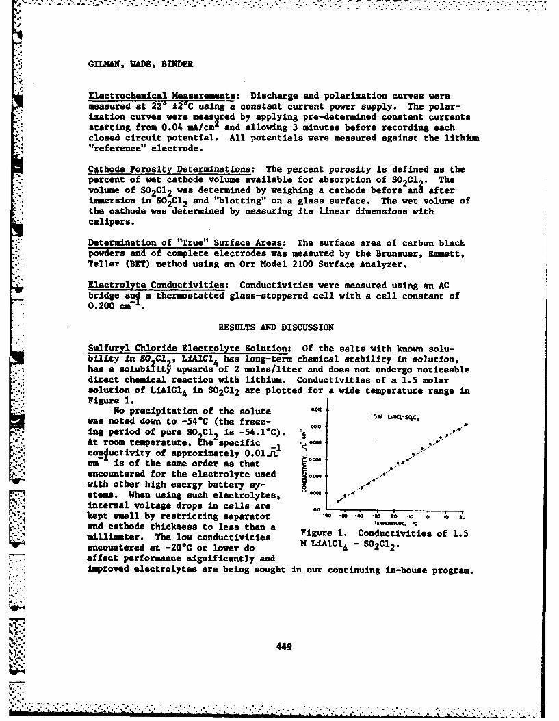
.4,i GILMAN, WADE, BINDER
Electrochemical Measurements: Discharge and polarization curves weremeasured at 22* ±2C using a constant current power supply. The polar-ization curves were measured by applying pre-determined constant currentsstarting from 0.04 mA/cm2 and allowing 3 minutes before recording each
.,1closed circuit potential. All potentials were measured against the lithi-"reference" electrode.
Cathode Porosity Determinations: The percent porosity is defined as thepercent of wet cathode volume available for absorption of S02C1,. Thevolume of S0 2 C12 was determined by weighing a cathode before an afterimmersion in S02C12 and "blotting" on a glass surface. The wet volume ofthe cathode was determined by measuring its linear dimensions withcalipers.
Determination of "True" Surface Areas: The surface area of carbon blackpowders and of complete electrodes was measured by the Brunauer, Emmett,Teller (BET) method using an Orr Model 2100 Surface Analyzer.
Electrolyte Conductivities: Conductivities were measured using an ACbridge an a thermostatted glass-stoppered cell with a cell constant of0.200 cm-f.
RESULTS AND DISCUSSION
Sulfuryl Chloride Electrolyte Solution: Of the salts with known solu-bility in SO2C12 , LIAICI4 has long-term chemical stability in solution,has a solubi yit upwards of 2 moles/liter and does not undergo noticeabledirect chemical reaction with lithium. Conductivities of a 1.5 molarsolution of LIAlCl4 in S02C12 are plotted for a wide temperature range inFigure 1.
No precipitation of the solute o0 , AC s +was noted down to -540C (the freez- 'S o o ',
ing period of pure SOCl2 is -54.10C). "..At room temperature, the specific oM
-1 -conductivity of approximately 0.01A.L .........
cm is of the same order as thatencountered for the electrolyte used .0"with other high energy battery sy-stems. When using such electrolytes,Internal voltage drops In cells arekept mall by restricting separator -W -0 -0 -0 0 ioand cathode thickness to less than a mmillimeter. The low conductivities Figure 1. Conductivities of 1.5
encountered at -20"C or lower do M LiAlCl4 - S02C12.affect performance significantly andImproved electrolytes are being sought in our continuing in-house program.
., 449
4 4 . . .- . o ° .-. . . . . . . . . ... . . . . .. °. . . . .-. ... . . ..o .. .. . . . .
? , : % % + '/ " +' + . +, . - + , , , , ' . -' .+ .' . . '. +' • .+ .. . . ., , . . . + . . '. -, + . . " . -" • . " .. . . . - ." .. , . ., . , .
GILIMAN WADE, BINDER
Lithim Anode in Sulfuryl Chloride Cells: A lithium electrode with afreshly prepared (by mechanical abrasion) surface shows little voltagepolarization for anodic current densities up to 40 mA/cm. On currentreversal, dissolved Lit is reduced to metallic lithium and deposited onthe surface of the lithium electrode in a highly dendritic form. Althoughprecise thermodynamic measurements have not been performed, one may con-elude that a fresh lithium electrode is close to reversible in a solutionof LIAlC14 in S02C12. The stability of the lithium electrode in SOC12 isdue to the formation of a self-limiting thin coating of LiC1, forms spon-taneously according to the reaction in Table I. On long-term storage, thatfilm apparently thickens and would introduce a "voltage delay" problem in abattery cell. This potential storage problem Is presently under investi-gation by a contractor (3).
Teflon-Bonded Cathode in the Li/S02C12 Cll: Electrodes for lithiumthionyl chloride cells are normally formulated with Shawinigan carbon blackand Teflon emulsion (normally 5-10% TFE n the dry electrode). Priorresults for sulfuryl chloride cells, using similar electrodes, producedrather discouraging results (4). In the present work, we experimented withseveral different types of carbon black powders and with the process ofelectrode fabrication. Table II lists the carbons studied along withproperties of the original powders and of completed electrodes fabricatedusing 16% TIE and a standard fabrication technique.
7T*51 n. Toi.i-oaded carbon ctbodes (16z Tfl)
Carbo Per gram Per cm2 of
load ofCaron electrode geo- I electrode--- vm of Cotas. eiei. Wail yd mtric area* porosity
Show"ISA-m comptoeed Decomgemtlon of ecetylooe 0.0194 661.26 67
* erco-60 steam-clvati. of charcoal 0.0046 301 14.4 64
Va telted MC-6310-4 Decomposltion of ol 0.0146 1000 14.6 a1
Columbia I 1670 Decoposltimo of oil 0.0104 100 12.5 75
a ueed on Omgh a vwith) area of electrode, one side.
an The resulting electrodes have "true" (SET) areas spanning more thanan order of magnitude and electrode porosities ranging from 64 to 872.Figure 2 presents polarization curves for such electrodes, with currentdensities based on the "superficial" area of the electrodes. From thefigure, it is clear that very significant differences exist between the
*W0450"
1-7 i
GILMAN, WADE, BINDER
electrodes, with "United" carbon black affording the best initial voltageover most of the current range. The results are replotted in Figure 3
:4 after basing the current density on the "true" (BET) rather than on the"superficial" surface areas. On that basis, it may be concluded thatalmost identical results are obtained for all of the carbons in the lower
-* range of current densities where mass transport effects may be expectednot to play a dominant role. This is consistent with the surface-chemicalmechanistic sequence to be discussed below.
0. .. .
&~ U nited XC-6310-4SV Shawinigan-502 Compressed sA United XC-63104 ' , 0 DARCO-C-60
"V Shavinigan-502 Compressed" .4. 1 Columbia HR 1670.>0 DARCO-G-6O
0 Columbia HR 1670 a
Current Density, NA/e2 (BASED ON GIoWZrUC AREA) Current Density, uA/cm2 (BASED ON a.E.T. AREA)
Figure 2. Polarization curves for TeE- Figure 3. Polarization curves forlon-bonded carbon cathodes in lithium- Teflon-bonded carbon cathodes insulfuryl chloride ' cells. Current den- lithium-sulfuryl chloride cells.sities based on "superficial" cathode Current densities based on "true"areas. (BET) surface areas.
Figure 4 shows that the capacity of the test cathodes depends directlyon the gross electrode porosity as measured by solvent absorption. Theporosities are determined, to some extent, by the inherent microscopic"structure" of the carbon powders. Shawinigan black, for example, is notedfor its highly developed acetylenic structure, carried over from the mole-cule from which it is originally derived.
From Figures 1-4 one can conclude that the "best" cathode would com-bine both high BET area and high porosity. Attempts were made to accom-plish these conditions, simultaneously, by formulating cathodes with mix-tures of Shawinigan black and the higher area carbons with unsatisfactoryresults. Success was achieved by varying the fabrication process in orderto increase the porosity of United carbon electrodes. Figure 5 presentsrepresentative discharge curves for different formulations. The use ofUnited Carbon and a "cold-compression" process (Trace 5, Figure 5) wasadopted as standard for the balance of this work. The electrode was
F further optimized with respect to teflon content (at 11% TFl). A typicalelectrode had a porosity of 87Z and a carbon loading of 0.024 gm/cm'.
;- 451
GILMAN, WADE, BINDER
~80.Y.%/
60
40 -
0 o 0ARCO-G-6020 l COLUIA I 1670
A UNITED XC-6310-4 (3) 53 SU ~ nW. ......ea .o .L . .---- ----Ji * V SH.WINIGAN.-50Z COMPRESSED ( L;; :: I: o: -o:
50 60 70 80 90 1
PERCENT POROSITY DlAOAGE TIRE,
" . Figure 4. Capacity-porosity rela- Figure 5. Discharge curves at currenttionship for Teflon-bonded carbon drains of 5 mA/cm2 for differently-cathodes (standard, "uncompressed"' formulated cathodes in lithium-sul-fabrication). furyl chloride cells.
Figures 6 and 7 compare performance of the cathodes of our Li/S02C12cell with that of the older Li/SOC12 system, which was previously the mostenergetic ambient temperature primary cell system known. Because anodepolarizations are small, the voltages are essentially those of a completepractical cell. Although the performance illustrated in Figure 6 and 7 isexcellent, there is still the possibility for significant improvements athigh currents and low temperatures and that is one thrust of our continu-ing battery research program.
• u.I " .. .. .., - a .,. , '
N
4 , (J, Q) C..... IX - /..I. S A/c.2
I , I (5) (c.,,K IVc,,.,-2 . • 1R Wk/c.2
7* 2 N S ~ CY~OC "M' M21 I 20 .-VC02 2 I
75.0 C' 2 6 4 0 15 1 0 N I IS 2'0 '2SuaCt Si,,.udc2 uo " .... ., DIX- Te,c (~,uIa.5 c
Figure 6. Comparison of cathodic Figure 7. Comparison of cathodic dis-polarization curves for lithium- charge curves for lithium-sulfurylsulfuryl chloride and lithium- chloride and lithium-thionyl chloridethionyl chloride cells, cells.
452
V *-.
GILMAN, WADE, BINDER
Electrode Discharge Products in the Li/SOCd Cell: The overall dischargereaction listed for the Li/SO2C12 cell in Table I vas deduced throughx-ray diffraction, gravimetric chloride determinations and volumetricdeterminations of SO2 gas release. First, it was determined that LiCi is,practically speaking, insoluble in the electrolyte solution employed here.Hence, discharged cathodes could be exhaustively washed with pure S02C12to eliminate entrained LiAlC14 , withoutaolubilizing LiC formed as aproduct in the cathode. Diffraction patterns for cathodes which werecarefully washed, dried and crushed revealed only cubic LiCl. Two cellsmade wih United carbon cathodes were discharged at a current density of5 mA/cm' to a cutoff voltage of 2 Volts. The cathodes were washed withS02C12, dried and quantitatively extracted with water. Aliquots of theaqueous solutions were potentiometrically titrated for C1 using a stan-dardized AgNO3 solltion. A small correction for occluded AlC14 was madeby determining A1+3 colorimetrically and subtracting four times that num-ber of equivalents. The corrected equivalents of Cf- were found equivalentto the coulombs of electricity passed, to within a 2Z tolerance. Thisestablishes that LiCl is the only ionic product of cell discharge and alsothat the LiC is quantitatively precipitated in the pores of the cathode.
To evaluate non-ionic discharge products, it was first determinedquantitatively that gaseous S02 is released during cell discharge. A cellwas then assembled with electrolyte which was pre-saturated with SO . Thecell was attached to a gas buret (using fluorocarbon oil as tc-hdisiace-ment liquid), and discharged at 5 mA/cm2 while monitoring the volume ofgas released. In duplicate experiments, it was established that one moleof gas was produced for every two equivalents of electricity passed.
The overall reaction listed in Table I is the simplest one consistentwith the analytical results reported above. The following individualelectrode reactions are consistent with the overall reaction:
anode: 2[Li -0 Li+ e]la)
cathode: 2Li+ + S02C12 + 2e-, 2LiC1 + SO2 (lb)overall: 2Li + S02Cl 2-2LiCl + SO2 (2)
E* - 3.909 V (30C)
As already discussed above, the capacity of the cathode is proportional to
its porosity. As is apparent from these findings, the porosity is required
in order to accommodate the LiCl precipitate while allowing continued goodtransport of the cathode reactant and of conducting ions.
The analytical results reported above contradict earlier reports (5)that Li2SO4 and molecular sulfur are major products of cell discharge. Itis felt that the earlier results may have resulted from a failure to avoidwater contamination early in the analytical procedure. The present resultsare particularly significant for their relevance to battery safety, inasmuch
453
. 9,'
V!
GILMAN, WADE, BINDER
as molten sulfur can react vigorously with lithium under conditions ofcell malfunction. This is potentially a very significant advantage of theLi/SO2C12 over the older Li/SOCd2 system (see Table I).
Cathode Hechanism in the Li/SO2Cl. Cll: Sulfuryl chloride is known (6)to dissociate into S02C12 accordinig to the following reaction:
s02C12 4PSO 2 + C12 (3)
Both gases are appreciably soluble in our electrolyte (1.09 and 0.62 molalfor 02 and Cl2 , respectively, at 240C as determined in this laboratory).Furthermore, as determined by W. Behl (7), of this laboratory, molecularC1 is more reactive than undissociated S02C 1 . Figure 8 shows that satur-ation of the electrolyte with either S02 or Cf2 produces a noticeable shiftin the cathode polarization curve. The particularly marked effect of SOimplies that the latter is acting by removing C12 as cathode reactant andshifting the equilibrium of reaction (3) to the left. A complete cathodemechanism, consistent with our observations, would involve the productionof C12 by reaction (3) followed by the cathodic reduction of C12 :
Cl2 + 2e- + 2Li+---u 2LiC1 (4)
Carbon is a known catalyst for reaction (3) and that would explain the im-portance of high electrode surface area to good electrode performance.
Quantitative information on reactionaEhjctmaui, (3), in the condensed phase, is de-
vCUcmv it .. sired for confirmation of the pro-£E&*C.ULWI SITMI ~posed cathode mechanism and as a
basis for future cathode improve-ments. Preliminary studies have
* *-96 .... . .. k been performed using ultraviolet13.8 "spectrophotometry. Figure 9 shows,.-., . ~3. -' l
:..: • that "aged" sulfuryl chloride ab-- - - - --- sorbs light with wavelengths less
0.1 1.0 1 than 460 mz, (the liquid appears yel-C,.,jm Drnn,. Oa ,Wm, a "laic M") low). The absorbance is diminished
Figure 8. Cathodic polarization by freshly-saturating with argon,curves of lithium-sulfuryl chloride and further diminished by saturatingcells containing gas-saturated elec- with SO2 (the latter does not absob-trolyte. light in this region of the spec-
trum). The absorbance is intensi-fied by adding C12. Comparison of the results suggests that the "aged" so-lution has undergone decomposition. Estimates of the rate of decompositioncan be made by recording the absorbance (e.g., at 400 Mu) vs time relation-ship for freshly degassed samples. Preliminary results reveal that, at300C, the homoseneous rate for the "neat" solvent is equivalent to lessthan 0.2 mh/=4 (exact rates depend on solvent purity) and, hence, wouldnot support good cathode performance at high current densities. In the
4
. .. . . . . . . . . . .
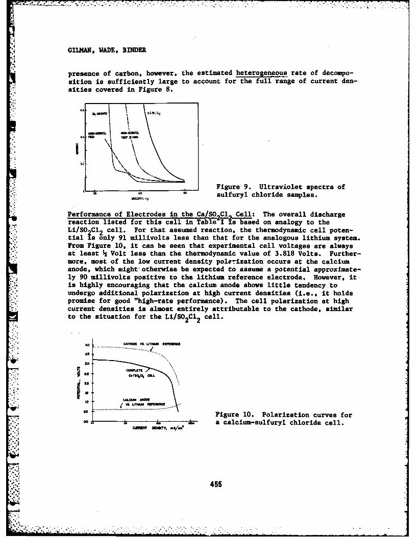
GILMAN, WADE, BINDER4
presence of carbon, however, the estimated heterogeneous rate of decompo-sition is sufficiently large to account for the full range of current den-sities covered in Figure 8.
-0.
\\ \&S IV, \ ,2
:--:_Figure 9. Ultraviolet spectra of
,. ,, sulfuryl chloride samples.
Performance of Electrodes in the Ca/SO Cl Cell: The overall dischargereaction listed for this cell in TableI is based on analogy to theLi/SO2C12 cell. For that assumed reaction, the thermodynamic cell poten-tial Is only 91 millivolts less than that for the analogous lithium system.From Figure 10, it can be seen that experimental cell voltages are alwaysat least 1 Volt less than the thermodynamic value of 3.818 Volts. Further-more, most of the low current density polerization occurs at the calciumanode, which might otherwise be expected to assume a potential approximate-ly 90 millivolts positive to the lithium reference electrode. However, itis highly encouraging that the calcium anode shows little tendency toundergo additional polarization at high current densities (i.e., it holdspromise for good "high-rate performance). The cell polarization at high
:,., current densities is almost entirely attributable to the cathode, similarto the situation for the Li/SO2 C1 2 cell.
aS ~ ~~ ...............
IsC&LwI WINOS
aFigure 10. Polarization curves fordo a calcium-sulfuryl chloride cell.
455
4....
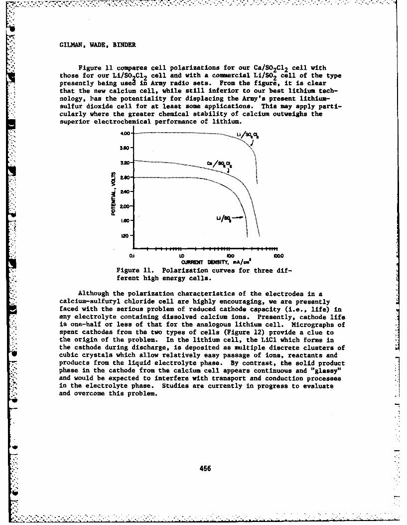
GILMAN, WADE, BINDER
Figure 11 compares cell polarizations for our Ca/S0 2C12 cell withthose for our Li/SO2C12 cell and with a commercial Li/SO2 cell of the typej 2presently being usea in Army radio sets. From the figure, it is clearthat the new calcium cell, while still inferior to our best lithium tech-nology, bas the potentiality for displacing the Army's present lithium-sulfur dioxide cell for at least some applications. This may apply parti-cularly where the greater chemical stability of calcium outweighs thesuperior electrochemical performance of lithium.
4.00 ........................................
3.60-
I o ........................ ....................... .
S. ................................
100
"= .00-
; :O IO MO-
CQMRNT MDESITY, mA/0m
Figure 11. Polarization curves for three dif-ferent high energy cells.
Although the polarization characteristics of the electrodes in acalcium-sulfuryl chloride cell are highly encouraging, we are presentlyfaced with the serious problem of reduced cathode capacity (i.e., life) inany electrolyte containing dissolved calcium ions. Presently, cathode lifeis one-half or less of that for the analogous lithium cell. Micrographs ofspent cathodes from the two types of cells (Figure 12) provide a clue tothe origin of the problem. In the lithium cell, the LiCl which forms inthe cathode during discharge, is deposited as multiple discrete clusters ofcubic crystals which allow relatively easy passage of ions, reactants andproducts from the liquid electrolyte phase. By contrast, the solid productphase in the cathode from the calcium cell appears continuous and "glassy"and would be expected to interfere with transport and conduction processesin the electrolyte phase. Studies are currently in progress to evaluateand overcome this problem.
456
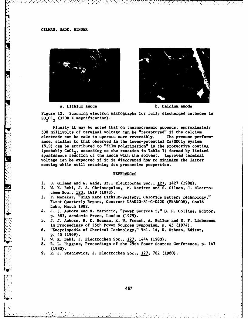
GILMAN, WADE, BINDER
a. Lithium anode b. Calcium anode
Figure 12. Scanning electron micrographs for fully discharged cathodes in02C 2 (3200 X magnification).
Finally it may be noted that on thermodynamic grounds, approximately500 millivolts of terminal voltage can be "recaptured" if the calciumelectrode can be made to operate more reversibly. The present perform-ance, similar to that observed in the lower-potential Ca/SOI 2 system(8,9) can be attributed to "film polarization" in the protective coating(probably CaCl2 , according to the reaction in Table I) formed by limitedspontaneous reaction of the anode with the solvent. Improved terminalvoltage can be expected if it is discovered how to minimize the lattercoating while still retaining its protective properties.
REFERENCES
1. S. Gilman and W. Wade, Jr., Electrochem Soc., 127, 1427 (1980).2. W. K. Behl, J. A. Christopulos, M. Ramirez and S. Gilman, J. Electro-
chem Soc., 120, 1619 (1973).3. F. Marakar, "High Rate Lithium-Sulfuryl Chloride Battery Technology,"
First Quarterly Report, Contract DAAK20-81-C-0420 (ERADCOM), GouldLabs, March 1982.
4. J. J. Auborn and N. Marincic, "Power Sources 5," D. H. Collins, Editor,p. 683, Academic Press, London (1975).
5. J. J. Auborn, R. D. Bezman, K. W. French, A. Heller and S. F. Liebermanin Proceedings of 26th Power Sources Symposium, p. 45 (1974).
6. "Encyclopedia of Chemical Technology," Vol. 14, K. Othmen, Editor,p. 45 (1969).
7. W. K. Behl, J. Electrochem Soc., 127, 1444 (1980).V 8. R. L. Higgins, Proceedings of the 29th Power Sources Conference, p. 147
(1980).9. R. J. Staniewicz, J. Electrochem Soc., 127, 782 (1980).
457
.7. :7 .
GLADEN & LINK
THER1AL CAMOUFLAGE OF FIXED INSTALLATIONS:PROJECT TIREX (U)
-' *CURTIS L. GIADEN, MR.LEWIS E. LINK, DR.
USAE WATERWAYS EXPERIMENT STATIONVICKSBURG, MS 39180
I. Introduction
1. Camouflage of fixed installations is a special problem because:
a. The facilities are static and their location and configura-tion are often well known.
b. Individual structures may be quite large and groups of struc-tures can cover an extensive ground area.
c. Few fixed installations have been constructed or sited prop-erly for the expedient addition of camouflage measures; simi-larly, new facilities seldom include camouflage in theirdesign criteria.
d. Very little attention has been focused on development ofmaterials and concepts for camouflage of fixed installationssince World War 1I.
Increased adversary air strength and advancements in target acquisitionand terminal homing system have placed a new premium on camouflage anddeception at fixed installations. The Corps of Engineers is addressingthis requirement in its fixed-installation camouflage research program.
2. The Corps research has considered a number of possible approachesfor camouflaging a fixed installation. Any given approach must considerboth camouflage technique and the scope of camouflage application. Tech-nique concerns alternative camouflage methods such as tone-down, shapedisruption, and decoys. Scope of application defines the degree to whichcamouflage is applied such as the number of structures or the proportionof the entire installation on which camouflage is used.
459
.-...
GLADEN & LINK
3. The most extensive application of camouflage would include anentire installation. This could involve a disguise of the presence of theinstallation (primarily to defeat surveillance systems) or to a lesserdegree an overall reduction in the conspicuousness of the installation todefeat target-acquisition systems. A less extensive approach would be toapply camouflage only to the critical elements of the installation andthose features in proximity to the critical elements that might be used toestimate their locations. Critical elements in this sense are thosenecessary for the survival of resources required to execute the opera-tional mission of the installation or to retaliate after an attack. Thelatter approach lends itself specifically to the defeat of target acquisi-tion and terminal homing devices used with manned fighter-bomber aircraft.
4. Manned fighter-bomber aircraft approaching at low altitudes andhigh 7ates of speed require a certain amount of time to locate specifictargets and lock-on with a weapon system. This can be translated to dis-tance; that is, the pilot, visually or with a target-acquisition aid, mustdetect and identify a specific target at a sufficient range from that tar-get to allow lock-on and accurate firing or weapon release. It is againstthis threat that camouflage of fixed installations can provide the mostcost effective counter and increase the survivability of an installation'scritical resources. The Corps' ongoing research emphasizes the develop-ment of thermal camouflage measures against this threat to complementexisting techniques used in the visual band.
5. Camouflaging structures to reduce their thermal contrast to thesurrounding terrain is particularly difficult because of the significantand at times rapid variations in both target and background thermal infra-red (IR) signatures. Targets can be warmer than the background during oneportion of the day and cooler a few hours later. A change in the weathercan reduce target-background contrast, eliminate it, or increase it withinhours or a fraction of an hour. Since many target-acquisition systemsutilize imaging sensors, the geometries (shape and texture) of the targetand background are also important considerations. Terrain areas surround-ing structures can vary considerably in their pattern and texture as per-ceived by thermal IR sensors. An area having variations in the percentageof grass cover and adjacent patches of trees may appear very uniform intone with subtle boundaries at one time and heterogeneous with significantdifferences in tone and texture both between and within the areas of grassand trees at another time. Effective camouflage of a structure withinsuch an area may require that the pattern and texture of the camouflagevary in phase with that of the background.
V 6. The growing threat posed by thermal IR imaging systems and heatseeking munitions and the almost complete dearth of information on thermalcamouflage of fixed installations are the impetus for the Corps' researchemphasis in this area. The interest in developing thermal camouflage
460
' GUlIN G LINK
technology I shared by many of our NATO allies and formed the basis forthe first major thermal camouflags field trial focused on fixed installa-tions. This paper provides an overview of the field trial called ThermalInfrared Experiment (TIM) and presents som preliminary results.
II. Overview of Project TIREX
A. Organization and Approach
7. In Februry 1979, members of NATO Working Group D of the SpecialGroup of Experts on Concealmnt, Camouflage, and Deception (NATO AC/243(CCD) WG(D)) agreed to cooperate in Project TREX. One objective of thetrial wse to evaluate the potential of a variety of materials and materialapplication concepts to reduce the vulnerability of critical elements atfixed installations to air attack by system using thermal ZR sensors.
8. Project TIRE participants included Denmark, the Netherlands, theUnited Kingdom, the United States, and West Germany. The U.S. Aruy Engi-near Waterways Experiment Station (WIS), Vicksburg, Mississippi, U.S.A.,had responsibility for overall coordination of project TIREX. Participa-tion in the program involved contributing samples of thermal camouflagematerial for testing, supplying measurement team for gathering fielddata, and supplying scientific personnel to analyze the data collected.The U.S. Air Force Base at Zweibruecken, West Germany, was selected as thesite for the field trial. Because of the size of the installation and thediversity of its structures, no effort was made to examine and treat thewhole installation or even significant parts of it. Instead, two generaltarget categories were decided upon and several targets in each categorywere examined. The two categorles considered were hot targets and coldtargets. Not targets were defined as buildings with internal heating andminimal insulation. Cold targets were unheated structures such as air-craft shelters and taxiways.
9. A two-pronged method of problem attack using a combination ofcomputer modeling and field experiments ws selected. The field experi-ment portion of the study was conducted in two phases. Phase 1 (Aug-Oct 79) involved the gathering of baseline temperature and thermal imagerydata at the field site. Phase 2 (Sep-Nov 80) involved a side-by-sidefield comparison test of various potential thermal camouflage materials.Computer modeling will be used to extend the field test results to otherclimatic conditions, to other camouflage materials, and to other camou-flage configurations. The final products will include initial guidancefor the design and application of thermal camouflage for critical elementsof fixed installations.
461
i i n ... .t , r ' it -' "i " "- ', '-" ' " *' --: _ . . . _ . : . , , .: . . .: i . __
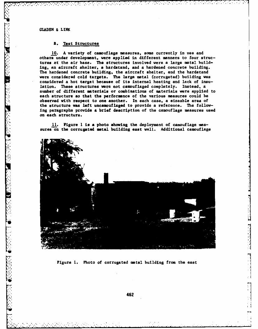
GIADEN & LINK
B. Test Structures
10. A variety of camouflage measures, some currently in use andothers under development, were applied in different manners to four struc-tures at the air base. The structures involved were a large metal build-ing, an aircraft shelter, a hardstand, and a hardened concrete building.The hardened concrete building, the aircraft shelter, and the hardstandwere considered cold targets. The large metal (corrugated) building wasconsidered a hot target because of its internal heating and lack of insu-lation. These structures were not camouflaged completely. Instead, anumber of different materials or combinations of materials were applied toeach structure so that the performance of the various measures could beobserved with respect to one another. In each case, a sizeable area ofthe structure was left uncamouflaged to provide a reference. The follow-ing paragraphs provide a brief description of the camouflage measures usedon each structure.
11. Figure 1 is a photo shoving the deployment of camouflage mea-sures on the corrugated metal building east wall. Additional camouflage
U
SFigure 1. Photo of corrugated metal building from the east
462
,.:
V
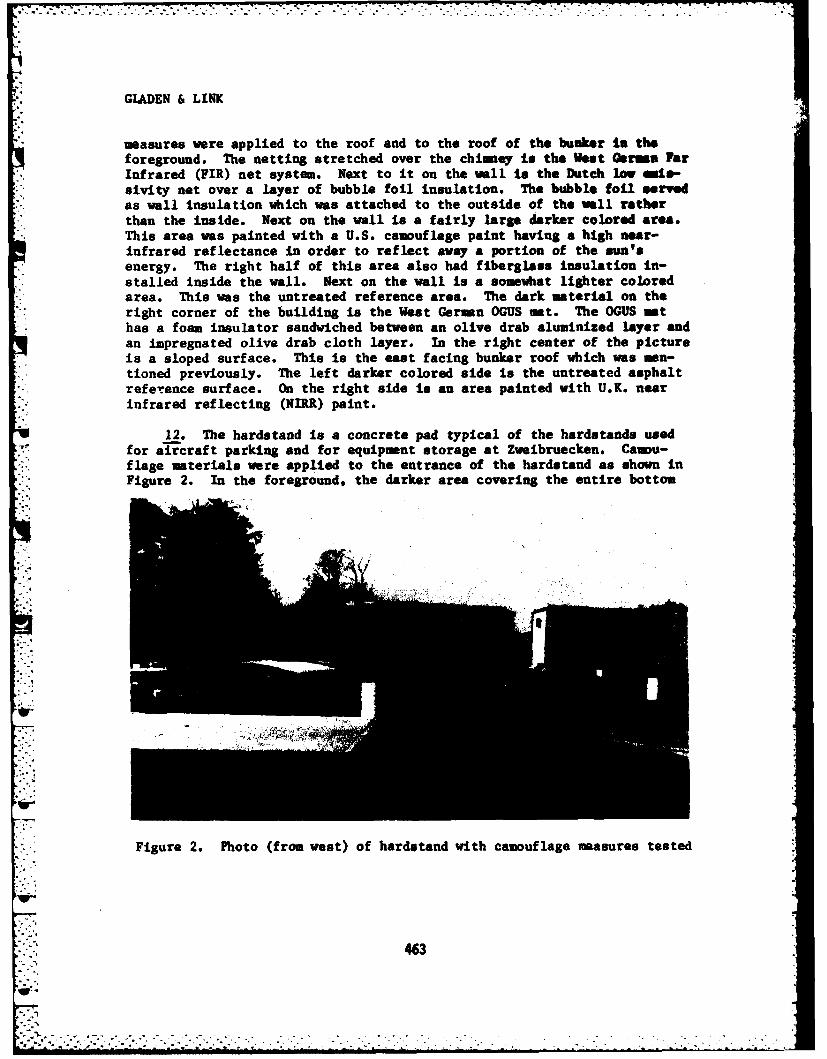
9." GLADEN & LINK
measures were applied to the roof and to the roof of the bunker in theforeground. The netting stretched over the chimney is the West Germsa FarInfrared (FIR) net system. Next to it on the well is the Dutch low smis-sivity net over a layer of bubble foil insulation. The bubble foil servedas wall insulation which was attached to the outside of the wall ratherthan the inside. Next on the wall is a fairly large darker colored area.This area was painted with a U.S. camouflage paint having a high near-infrared reflectance in order to reflect away a portion of the sun'senergy. The right half of this area also had fiberglass insulation in-stalled inside the wall. Next on the wall is a somewhat lighter coloredarea. This was the untreated reference area. The dark material on theright corner of the building is the West Germn OGUS mat. The OGUS mathas a foam insulator sandwiched between an olive drab aluminized layer andan impregnated olive drab cloth layer. In the right center of the pictureis a sloped surface. This is the east facing bunker roof which was men-tioned previously. The left darker colored side is the untreated asphaltreference surface. On the right side is an area painted with U.K. nearinfrared reflecting (NIRR) paint.
12. The hardatand is a concrete pad typical of the hardstands usedfor alrcraft parking and for equipment storage at Zweibruecken. Caou-flage materials were applied to the entrance of the hardstand as shown inFigure 2. In the foreground, the darker area covering the entire bottom
Figure 2. Photo (from west) of hardstand with camouflage measures tested
463
. . ..
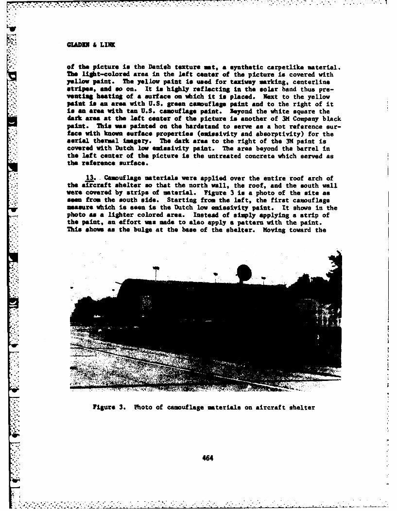
GLOWEN & LIK
of the picture is the Danish texture mat, a synthetic carpetlike material.Te light-colored area in the left center of the picture is covered withyellow paint. The yellow paint is used for taxiway marking, centerlinestripes, and so on. It is highly reflecting in the solar band thus pre-venting heating of a surface on which it Is placed. Next to the yellowpaint is an area with U.S. green camouflags paint and to the right of itIs an area with tan U.S. camouflage paint. Beyond the white square thedark area at the left center of the picture is another of 3K Company blackpaint. This was painted on the hardtand to serve as a hot reference sur-face with known surface properties (emissivity and absorptivity) for theaerial thermal Imagery. The dark area to the right of the 3M1 paint iscovered with Dutch low ewissivity paint. The area beyond the barrel inthe left center of the picture is the untreated concrete which served asthe reference surface.
13.. Camouflage materials were applied over the entire roof arch ofthe aircraft shelter so that the north wall, the roof, and the south wallwere covered by strips of material. Figure 3 is a photo of the site asseen from the south side. Starting from the left, the first camouflagemeasure which is seen is the Dutch Io emissivity paint. It shows in thephoto as a lighter colored area. Instead of simply applying a strip ofthe paint, an effort was made to also apply a pattern with the paint.This shows as the bulge at the base of the shelter. Moving toward the
. . .. .. .........
'."-. V,
Figure 3. Photo of camouflage materials on aircraft shelter
464
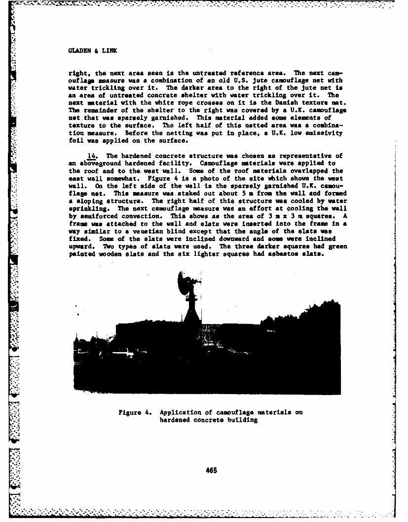
GLADEN & LINK
right, the next area seen is the untreated reference area. The next cam-ouflage measure was a combination of an old UoS. jute camouflage net withwater trickling over it. The darker area to the right of the jute net isan area of untreated concrete shelter with water trickling over it. Thenext material with the white rope crosses on it is the Danish texture mat.The remainder of the shelter to the right was covered by a U.K. camouflagenet that was sparsely garnished. This material added some elements oftexture to the surface. The left half of this netted area was a combina-tion measure. Before the netting was put in place, a U.K. low emissivityfoil was applied on the surface.
14. The hardened concrete structure was chosen as representative ofan aboveground hardened facility. Camouflage materials were applied tothe roof and to the west wall. Some of the roof materials overlapped theeast wall somewhat. Figure 4 is a photo of the site which shows the westwall. On the left side of the wall is the sparsely garnished U.K. camou-
flage net. This measure was staked out about 5 m from the wall and formeda sloping structure. The right half of this structure was cooled by watersprinkling. The next camouflage measure was an effort at cooling the wallby semiforced convection. This shows as the area of 3 m x 3 m squares. Aframe was attached to the wall and slats were inserted into the frame in away similar to a venetian blind except that the angle of the slats wasfixed. Some of the slats were inclined downward and some ware inclinedupward. Two types of slats ware used. The three darker squares had greenpainted wooden slats and the six lighter squares had asbestos slats.
Figure 4. Application of camouflage materials onhardened concrete building
465
. - ••
GLADEN & LINK
15. The light-colored area to the right of the slate was the un-treated wail reference area. Next to it is a combination measure. Thetop half of the wall was painted with Dutch low emissivity paint. Thenhalf of this area was covered by a Dutch camouflage net which was sus-pended vertically at a distance of about 1 m from the wall. The lowerhalf of the wall was covered by Danish texture mat which was attacheddirectly to the wall. Next to this measure is another combination mea-sure. Beneath the Dutch camouflage netting seen in the photo is a U.S.furnished mat made up of space blankets, a commercially available thermalblanket. The space blankets were hung with the shiny side facing out inorder to form a low emissivity surface. The last measure on the west wallwas also a combination measure. A U.S. thermal blanket was draped downnext to the wall and then a U.S. camouflage net was stretched out over itaway from the wall. This measure appears in the photo immediately to theright of the white wall column next to the trees.
C. Ground Measurements
16. The ground measurements were made to characterize site condi-tions, thermal characteristics of the camouflaged and uncamouflaged struc-tures, and background features over diurnal cycles and in differentweather conditions. Four types of ground data were obtained: weather,feature temperature, feature reflectance, and imagery.
.17. The weather data consisted of measurements of solar insolation,wind speed, wind direction, relative humidity, and air temperature. Mea-surements were recorded every 30 minutes with each value representing anaverage value for the previous 30 minutes. Measurements were recorded onmagnetic tape cassettes for subsequent analysis.
18. Contact surface temperature measurements were made for most cam-ouflage measures, uncamouflaged reference areas, and adjacent backgroundareas using thermistors attached to the material surfaces. The thermis-tors were attached to data logger and recorder systems similar to the oneused for the weather data. Temperature values were recorded every 30 min-utes for the duration of the experiment.
19. Radiometric temperature values were obtained manually by use ofan AG-Thermopoint TPT 80 Radiation Thermometer, a Wahl Heatspy RadiationThermometer, and a Barnes Engineering Instatherm hand-held measurementdevice. A digitron Model 1751 Contact Thermometer was used to supplementthese devices. Radiation temperatures were obtained over selected diurnalcycles spaced over the extent of the field data collection. Periodic mea-surements were made of the surface radiometric temperatures ot the indi-vidual camouflage materials, uncamouflaged reference areas, and backgroundfeatures adjacent to the structures camouflaged.
466
°, ... .
. . . . . . .. . . .
"7I
GIADEN & LINK
20. Optical reflectance measurements for the individual camouflagemterials (in situ), reference areas, and background features were madeperiodically by the various scientific teams. Additional material proper-ties were determined through laboratory analyses by IABG Corporation,West Germany. The optical reflectance measurements were made with anintegrating quantum radiometer/photometer providing hemispherical reflec-tance for solar (.4 to 1.2 pa), near infrared (0.67 to 0.85 um), andvisual (standard response of the human eye) bands.
*' 21. Thermal IR imagery was obtained from preestablished ground sta-tions by two West Germany teams (FfO and IABG) and teams from the Nether-lands, Denmark, and the United States. The thermal IR imagery was ac-quired with modified AbA Thermovision Systems (Denmark and West Germany),Inframetric (United States), and a privately designed system used by theNetherlands team.
22. The image information was recorded on magnetic tape for most ofthe systems with the exception of the IABG system, which used an analog todigital converter to generate digital records of the imagery. All mea-surements were made in the 8- to 14-Am spectral band with the exception ofthose made by the Netherlands, which were made in both the 3- to 5-jrm and8- to 14-um spectral bands. The various scientific teams acquired imageryover selected diurnal cycles to provide relatively uniform coverage overthe full period of the field data acquisition. Since all teams acquiredimages from the same positions and at approximately the same times duringthe diurnal cycle, the imagery collected form a compatible data set thatcan be used to examine the performance of the respective camouflage mea-sures over diurnal cycles and for a variety of weather conditions thatspan the 15 Sep to 10 Nov time period.
D. Aerial Data
23. Aerial overflights were made to acquire both visual and thermalIR imagery. The visual imagery consisted of conventional panchromaticaerial photography. Two types of thermal IR imagery were obtained:vertical line scan imagery and forward-looking infrared (FLIR) imagery.Vertical line scan Imagery was acquired by U.S. Air Force tacticalreconnaissance aircraft. FLIR imagery was acquired by the West German FfOteam using a Honeywell mini-FLIR system. The team acquired simulated FLIRimagery with the Inframetrics imaging system mounted in a helicopter. Alimited amount of FLIR imagery was acquired in 1979 prior to the applica-tion of camouflage materials by a U.K. aircraft. The FLIR imagery wasobtained at different times of day and along preselected flight paths.
467
.L-e..r~~~~~gt C-C.r *W-'. -''. '.- .' :. .
GIADEN & LINK
III. Data Analysis
A. Analysis Approach
24. The major objectives of the data analysis were to (1) evaluatethe pjerformance of the various camouflage materials for contrast reduc-tion, both visual and thermal IR; and (2) evaluate the potential of thevarious camouflage measures (materials applied in specific ways) to reducethe detectability of specific types of structures for a variety of timeand weather conditions. The analysis of contrast reduction potential isbeing accomplished primarily with the ground radiometric temperature,reflectance, and contact temperature data. The analysis of detectabilityreduction potential is being accomplished primarily with imagery data sup-plemanted by modeling and simulation techniques.
25. Analyses of the data collected during the 1979 and 1980 fieldtrials has been ongoing by scientific teams from each nation. The analy-sis of contrast and reduction potential is largely completed, while theanalysis of detectability reduction potential is ongoing. Because of thesheer volume of data collected by the various scientific teams, it ispractical only to present a few example or representative analyses in thispaper. The analyses presented are those accomplished by WES personnel onthe U.S. ground based radiometric temperatures, reflectance, and contacttemperature data for the aircraft shelter.
B. Analyses of Radiation Temperature Data
26. For each data point (set of instrument readings), an averagetemperature of the material being examined was computed by adding the tem-perature readings from the various instruments together and dividing bythe number of instruments used. Next, the absolute value of the tempera-ture difference between the camouflage or reference material and itsappropriate background material (grass or trees) was calculated. Two mea-sures of camouflage effectiveness were calculated based on these absolute
.. value calculations. The first of these measures was a daily sum of theabsolute values for each camouflage measure and each reference surface.This provides a measure of the total daily temperature differences betweenthe camouflage or reference material and its background. The second of
V these measures was the daily sum for each camouflage material divided bythe daily sum for its appropriate reference material. This quotient wassubtracted from one. This measure compares the camouflage and referencematerials. If the result of this calculation is one, then the camouflageis perfect. However, if the result of this calculation is less than zero,then the camouflage material is less effective than the untreated refer-
.w ence surface. TabLe I presents the results from the aircraft shelter for -three data collection days. The last columns in the table provide overall
* -., measures for all three days. Based on these data the wet concrete and wet
w
1.'1468
- .1
" "" ~........""................... . ' " , ',",_ -"=_.,- "...... - -
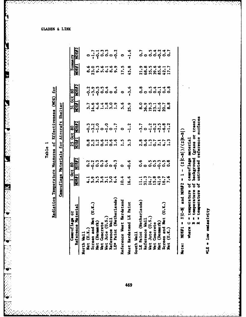
GLADEN & LINK
4. cn . -4 - c - k in Go %0 O~N c c
v $ G 0 %O'Q Ui- 40-4 a - -0 N % -4 $ $
P4 0[h ! 0!~f- -t 0! 0 V! -'t
001 0 C4 40 0 00 0 C4 0000000
to0%400 00 o$04A-%rI4 V-4( -I 4t4~4IA IAIA 04 O%(0440
di4
V ~ N 0 C; N 0. 0* 0 0 4
4.1 be Obi ": 11 . . . .U14 00 0CV en-4 04 4. CW040N 4 414 4
.0 w 41 v d
~ 0-4 V -0
LO 14 W4 0
1.469
't -. . . -• -.
GIADEN & LINK
jute (old U.S. camouflage net) were the most effective camouflage measuresdeployed on the north wall. On the south wall, the British camouflage netwas the most effective camouflage measure, followed closely by the Dutchlow emissivity paint. The result for the British net may be misleadingbecause it was shaded from direct sunlight during portions of the day.
C. Analyses of Reflectance Data
*27. A fairly simple performance analysis technique was also used forthe reflectance data. First, an appropriate natural background material(grass) was selected. Second, reasonable bounds were determined for thesolar, near IR, and visual reflectances of grass. These bounds weredetermined by selecting the minimum and the maximum grass reflectancesmeasured. The bounds established were as follows: solar reflectance,19 to 34 percent; near IR reflectance, 27 to 37 percent; visual reflec-tance, 5 to 9 percent. The third step in the analysis process was toexamine the reflectances of the materials to assign them into two catego-ries, those materials judged to have camouflage potential and those judgedto be camouflage deficient.
28. Materials with camouflage potential had to meet three require-ments. Their average reflectance had to be within the established reflec-tance bounds of the background, their average reflectance had to be higherthan that of the reference for the solar and/or near IR bands and lowerfor the visual band. These requirements lead to materials which have cam-ouflage potential in both the thermal and the visual portions of the spec-trum. Materials with high solar and near IR reflectances will usuallyabsorb less of the sun's energy. Thus, they will stay cooler and be goodfor thermal camouflage. Materials with low visual reflectance willre-flect less of the incident sunlight back to the observer and hence will begood for visual camouflage. Table 2 is the summary table for the aircraftshelter reflectance data. From the table one can see that only the Dutchlow-emissivity paint was judged to have overall camouflage potential.Generally, the other materials were Judged deficient because their solarand near 1R reflectances were too low.
D. Analyses of Contact Temperature Data
29. The analysis method used for the contact temperatures was nearlythe same as that used for the radiometric temperatures. However, therewere several differences. The temperature of the background material wasnot grass temperature, but rather air temperature measured at each site.Air temperature is a reasonable approximation of natural background tem-peratures (e.g. trees and grass). For the contact temperature devices,48 data points per day were collected and contact temperatures were col-
- * lected on 55 days. For each data point (temperature sample), an average. temperature of the material being examined was computed by adding the
470
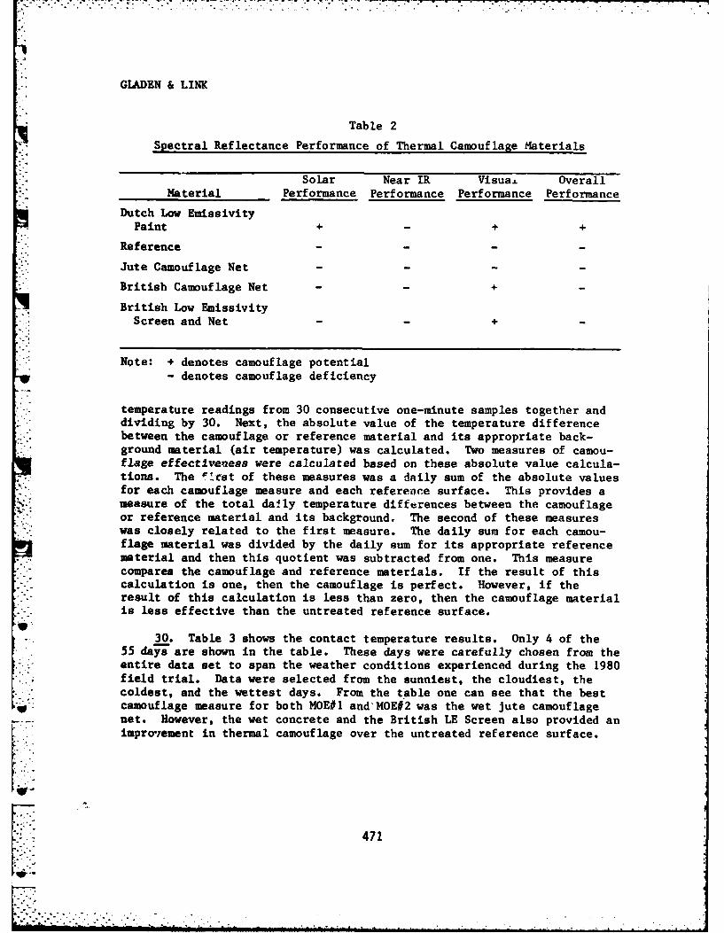
GLADEN & LINK
Table 2
Spectral Reflectance Performance of Thermal Camouflage M4aterials
Solar Near IR Visua. OverallMaterial Performance Performance Performance Performance
Dutch Low EmissivityPaint + - + +
Reference
Jute Camouflage Net ....
British Camouflage Net - - +
British Low EmissivityScreen and Net -
Note: + denotes camouflage potential- denotes camouflage deficiency
temperature readings from 30 consecutive one-minute samples together anddividing by 30. Next, the absolute value of the temperature differencebetween the camouflage or reference material and its appropriate back-ground material (air temperature) was calculated. Two measures of camou-flage effectiveness were calculated based on these absolute value calcula-tions. The 0., st of these measures was a daily sum of the absolute valuesfor each camouflage measure and each reference surface. This provides ameasure of the total daily temperature differences between the camouflageor reference material and its background. The second of these measureswas closely related to the first measure. The daily sum for each camou-flage material was divided by the daily sum for its appropriate referencematerial and then this quotient was subtracted from one. This measurecompares the camouflage and reference materials. If the result of thiscalculation is one, then the camouflage is perfect. However, if theresult of this calculation is less than zero, then the camouflage materialis less effective than the untreated reference surface.
30. Table 3 shows the contact temperature results. Only 4 of the55 days are shown in the table. These days were carefully chosen from the
. - entire data set to span the weather conditions experienced during the 1980'. field trial. Data were selected from the sunniest, the cloudiest, the
coldest, and the wettest days. From the table one can see that the best": camouflage measure for both MOE#1 and'MOE#2 was the wet Jute camouflage. net. However, the wet concrete and the British LE Screen also provided an
improvement in thermal camouflage over the untreated reference surface.
471
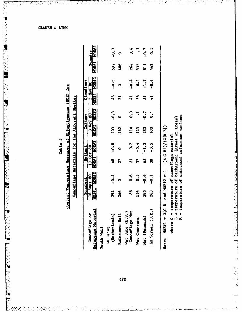
GIADEN &LINK
$ . k% - 0 %C -4 -4
"4 PR
-4
0 4' -J 1 $ $ . .
4.4 *Cc 04 0 0 4"'4 14.4
USn W ~ V 11.4
(A 0 , 6 !0!- C 4j o W
4 0 s M.414XC 0'. 0 -C4(t 7 O1
014 1 I I
g4 .R" "k 0 a " 0U3 $I 4 14
00 ~0 C,4,A0
4J ~ $ -A20 U0 0 0 (V0 N4 z 4f1 0
00 I 0)
4 04 .a.~~4j 0
"4472
''-- ': -' ''--'-''; - " -' " '. . ":. . ; _" . -.. " ". . " " . . ." : "
GLADEN & LINK
IV. Concluding Remarks
31. This paper has presented an overview of Project TIREX as well asa sampling of some of the results for one of the structures on which cam-ouflage materials were tested. The examples presented were limited toanalyses of contrast reduction potential in both the visual and thermal IRbands. The results are indicative of the results of the complete dataset. Few materials exist that offer an ability to completely reduce thecontrast of a structure to its natural surround. While many materialsoffer significant thermal or visual contrast reductions, none were idealfor simultaneously providing the desired reduction in both bands. Thisindicates a continuing need to develop better materials and applicationsconcepts.
32. While the results of ground-based data analyses may appear dis-couraging, when coupled with the initial imagery analyses the picture isnot so bleak. Structures that are not extremely hot targets, such as air-craft shelters and hardened concrete structures, are detectable primarilyby their individual shapes. The clever use of many of the existing mate-rials to accomplish shape disruption can be very effective in reducing thedetectability of those structures. The ground-based data provide a valu-able quantitative data base to aid in the design of material applicationconcepts. These concepts will allow use of these materials for modifyingthe appearance of structures to reduce their vulnerability to attack bythermal IR devices. Combinations of materials may provide significantreduction in the vulnerability of structures to both visual and thermal IRtarget acquisition aids. Insulating materials can have a significantimpact on the detectability of hot targets ruch as the heated corrugatedmetal building investigated.
33. Project TIREX will provide the first available systematic guid-ance for thermal camouflage design. While a considerable amount of devel-opmental work is still required, a very substantial foundation will heavailable to proceed rapidly to the full camouflage capability needed toaddress the modern threat.
473
. .- . . . .. . . .4
GOICOECHEA, KROUSE & ANTLE
AN APPROACH TO RISK AND UNCERTAINTYIN BENEFIT-COST ANALYSIS
OF WATER RESOURCES PROJECTS
AMBROSE GOICOECHEA, Ph.D.International Water Resources Institute
School of Engineering andApplied Sciences
George Washington UniversityWashington, DC
MICHAEL R. KROUSE-' Institute for Water Resources
U. S. Army Corps of EngineersFort Belvoir, Virginia
LLOYD G. ANTLE, Ph.D.Institute for Water ResourcesU. S. Army Corps of Engineers
Fort Belvoir, Virginia
1. INTRODUCTIONTraditionally, many benefit-cost studies in water resources planning
have been conducted under the assumption that the "most likely" or the "ex-pected" values of benefits and costs provide an appropriate economic basisfor the evaluation and comparison of alternative project plans. It is notalways acknowledged that estimates of those benefits and costs can varyover a range of values, and that study recommendations ought to reflect,somehow, the likelihood of estimates over their respective ranges. Evenwhen the effort is made to consider parameter ranges, it is not clear as tohow to proceed with the analysis-what analytical tools are to be used, andwhat tradeoffs to generate in order to assist in the decision-makingprocess.
President Carter reinforced the need to develop systematic proceduresfor the analysis of risk and uncertainty in his directions to the Water re-sources Council (WRC) on June 12, 1978- to produce guidelines under whichFederal Water Resources agencies conduct benefit-cost analysis. As a re-sult, the WRC outlined a project evaluation procedure (May 24, 1979) to
475WIl.

GOICOECHEA, KROUSE & ANTLE
assist planners deal with aspects of risk and uncertainty. In that proce-dure it was suggested that "a range of reasonably likely outcomes can bedescribed by using sensitivity analysis-the technique of varying assump-
• tions as to alternative economic, demographic, environmental and other fac-tors, and examining the effects of these varying assumptions on outcomes ofbenefits and costs." Furthermore, it was suggested to " ... characterizethe range of outcomes with a set of subjective probability estimates.Where it is appropriate to do this, methods for manipulating the subjectiveprobability estimates can then be used. However, if numerical estimates ofsubjective probability are given, it should be made clear in the projectreport that these are subjective and thus do not have the same objective
basis that characterizes. a long hydrologic record ... ". The outline went."on to suggest some general concepts to account for differences in risk and
uncertainty among project purposes and costs, time periods, and stages ofplanning.
Responses to the above guidelines deemed the effort unsatisfactory, asnoted in the "Federal Register of December 14, 1979 (pg. 72896). The prin-cipal thrust of the comments was that, "while it provided a clear statementof the problem and basic principles of risk and uncertainty in water re-sources planning, it failed to provide a usable procedure." The procedureas written was judged too general, permissive rather than directive, andlacking in instructive detail. Commenters noted "the omission of acceptedmathematical and probabilistic methodologies and the failure to identifyand list key factors to which benefit-cost evaluation is sensitive."
This heightened awareness of the role of risk and uncertainty in waterresources planning motivated the work reported in this paper. Specifical-ly, we have three objectives: (1)-to raise some issues and concerns aboutthe possible impacts of risk and uncertainty considerations on the prepare-tion and documentation of feasibility studies, the development of alterna-tive plans, the complexity of the decision-making process, and the time re-quired for that process to evolve, (2) to identify sources of risk anduncertainty in water resources planning, (3) to investigate the computa-tional requirements of a probabilistic approach to benefit-cost analysis,as well as its potential usefulness (or lack of it) in the evaluation ofalternative projects.
-0 2. SOURCES OF RISK AND UNCERTAINTYA distinction is made in defining the terms "risk" and "uncertainty,"
(Water Resources Council, Hay 24, 1979, pg. 30196). Situations of risk aredefined as those in which the random nature of potential outcomes can bedescribed in reasonably well-known probability distributions. In situa-tions of uncertainty, on the other hand, probability distributions are notknown and their estimation would be a predominantly subjective exercise.However, the distinction between risky and uncertain situations is not usu-ally a crisp one; rather, it is a matter of degree.
4
* - 476
2o , , , . .. .. , . ,-. -,. . . . . , . -. . . - . . - .
GOICOECHEA, KROUSE & ANTLE
Risk is usually associated with our understanding of physical phenom-ena for which the probability of occurrence of an outcome can be estimatedin a relatively objective manner (i.e., through the use of hydrologic rec-ords and similar data banks). When the assertion is made that an outcomewill take place with a probability of P, the term risk is used to denotethe probability (1-P) of other outcomes. Uncertainty, on the other hand ismore closely associated with physical phenomena, socio-economic interac-tions, environmental response, pollutant effects on health, and other situ-ations where our understanding is limited. These phoenomena and events arenot inherently random, but they are relatively poorly understood. The termuncertainty is used, then, to reflect the subjective nature of the proba-bilities when these are assessed.
Incorporation of risk and uncertainty considerations in the decision-making process, then, calls for the identification of sources of R & U, re-duction of R & U whenever possible, the generation of benefit-cost-risktradeoffs, and public involvement. Risk can be reduced in some instancesby collecting additional data and using the full length of available his-torical records (e.g., hydrologic records), increasing safety factors indesign (which increase costs, in turn), selecting system performance mea-sures with better-known characteristics, and by using more refined analy-tical techniques.
3. EXISTING AGENCY PROCEDURES FOR R & UWater resources agencies, in general, allow for elements of risk and
uncertainty in the decision-making process. This process often extends-: -over several decades involving several feasibility studies, numerous re-
quests for additional information, and the scrutiny of a chain of decisionmakers (agency review groups, political representation, and the generalpublic).
In the case of the U.S. Army Corps of Engineers (which is of particu-lar interest to the authors) the planning process starts with an assessmentof needs, and these are reassessed many times before the project is con-structed, and even many times after it becomes operational. Planners donot have much difficulty in documenting existing conditions and problems,but it becomes extremely difficult to characterize future conditions aswell as the benefits and costs associated with those conditions. Projec-tion of trends into the future become a complex and troublesome task. Theyare complex because they require an attempt to model and relate economic,social, demographic and political interactions over extended periods oftime. Also, these interactions are frequently simplified to keep the model(e.g., computer program, or set of analytical tools) manageable, thus fur-ther increasing the uncertainty inherent in the model projections.
.
I I - . . . . .l . .i ' i li i i.bi.m
GOICOECHEA, KROUSE & ANTLE
Agency review procedures are aimed at sorting out the conditions whichinfluence the design of alternative plans for a project and that have a ma-jor impact on benefit-cost (B/C) ratios. When a project report clears pre-liminary reviews at Corps field divisions and at Office of the Chief of En-gineers (OCE), the Board of Engineers for Rivers and Harbors (BERH) staffproceeds to review the project recommendations, project analysis, assess-ment of needs, and adherence to institutional policy. At this stage in thereview, special emphasis is placed on the analysis of safety aspects of de-sign criteria, and whether a project recommendation is supported by compe-tent B/C analysis. Projects that exhibit a B/C > 1.0 will tend to be fa-vored generally (there are other non-economic criteria to consider, aswell, as will be discussed later) over those projects with a B/C < 1.0.
If project justification is close (e.g., B/C is only slightly greaterthan 1.0), a determined examination of sources of risk and uncertainty maybe made to discern whether the recommendation is likely to survive long-runtrends toward higher discount rates, and whether demographic and economicprojections are consistent with trends forecast by the Office of BusinessEconomics Research Service (OBERS). In addition, recommendations by theChief of Engineers, the Secretary of the Army, and the Executive Office ofthe President may request that the project be subjected to restudy beforeadvanced engineering funds are approved.
As stated early in the paper, the need to develop systematic proce-
dures for the analysis of R & U has been perceived, however, and it may be
appropriate now to inquire about the nature of the additional informationto procure and document. Effective ways of displaying, "digesting" and in-tegrating that Information into the decision-making process become impor-tent also, particularly at the levels of (1) field division, (2) Board of
Engineers of Rivers and Harbors, and (3) public participation.
4. PROBILITY DISTRIBUTIONThe procedure presented in the next section requires that a probabil-
ity distribution be computed for each benefit and each cost component ofthe economic analysis. Such a distribution function would be defined overthe range of values of a particular cnmponent, and it would be character-ized by an average or mean value, and a variance. Once the various proba-bility distributions have been generated, the next step is to aggregatethem statistically into some measure of economic performance (e.g., netbenefits, B/C ratio, other).
For many problems there are available sufficiently long historicalrecords to estimate probability distribution or relative frequencies of oc-currence of the input parameters of interest. This Is true particularly ofinput parameters that relate to the risk portion of the analysis - numberof rainfall events in a given region within a year, intensity and duration
478
• , ,. . , .. .+ -. . o . -. , .- .-o - - - .- - , .. - . ... _ - . . . - . . . : • " i " a ,
GOICOECHEA, KROUSE & ANTLE
of rainfall events, amount of.runoff, etc. These distributions would be ofan objective nature, based on available records, and fairly reliable. How-ever, probability analysis with many economic or demographic variables suchas population projections, price elasticity, demand for recreation activi-ties, etc., often depends substantially on subjective estimates. Subjec-tive probability distributions are thus inferior to objective probabilitydistributions but invariably preferable to the option of omitting a measureof uncertainty altogether.
The suggested procedure begins with three estimates of possible valuesfor each input component (e.g., benefits and costs): an expected Value, anoptimistic vaZue,and a pessimistic value. The expected value is the valuethat is likely to occur, on the average, most often if the activity (e.g.,flood event, extent of recreation use, time required to complete a task,etc.) could be repeated a number of times under similar circumstances. Anoptimistic value is the maximum benefit (or minimum cost) that could berealized if "everything went right" - schedules are met, costs of buildingmaterials are accurately assessed, demand for recreational uses material-izes, etc. Finally, a pessimistic value is the minimum benefit (or maximumcost) that could be realized if "everything went wrong." Effectively,then, the optimistic and pessimistic values identify the range of possiblevalues for a given input component. Additionally, it is suggested in thisprocedure that the range representia "95 percent confidence interval,"i.e., 95 percent of the time the actual value would fall within the speci-fied range.
Once the three parameter estimates are prepared, it is possible to usethem to estimate the "mean! and the "variance." There remains, then, thematter of specifying the "shape? of the distribution to be able to talkabout the probability of that input parameter realizing a particular value
*] within its range.
-. Gamma Distribution
* A candidate is the gamma distribution of the form:
x/B
f(x) = • for 0 <x, (1)wt r(a)B
0 0, elsewhere
where a and 8 are the parameters that determine the general shape of this.- function. The first two moments of t4ts function are:
-: mean, E(X) = : a (2)
479
F-! . ... ...
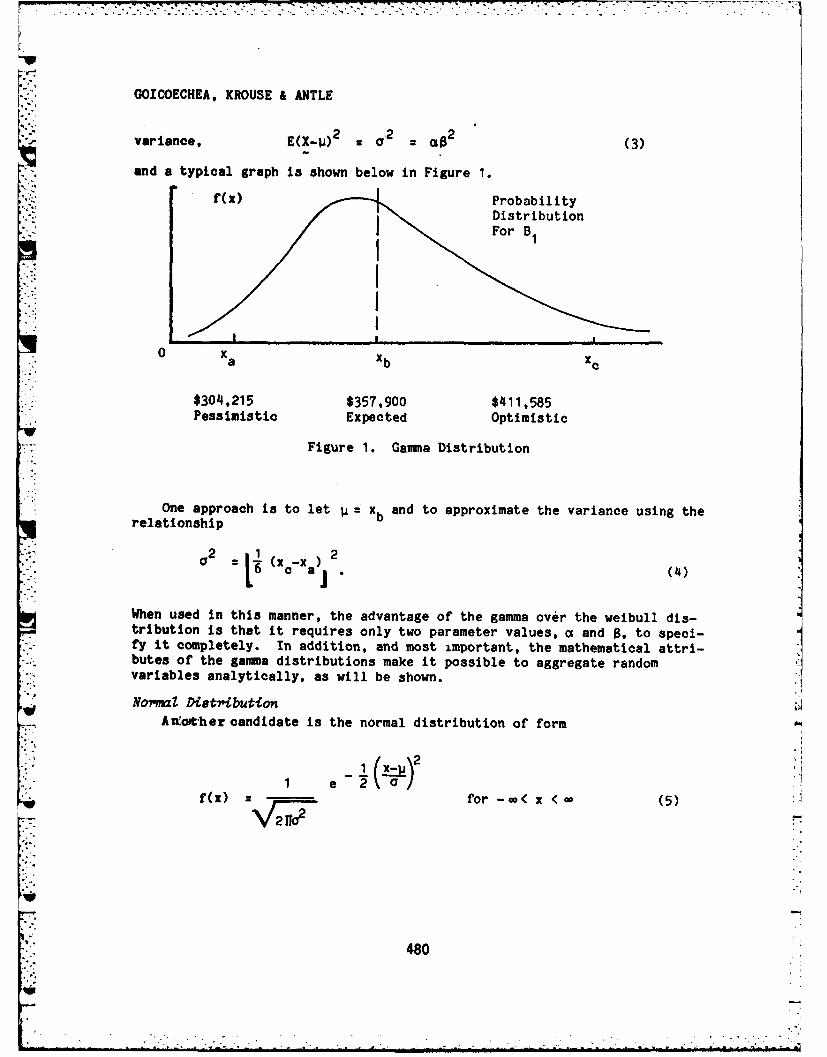
GOICOECHEA, KROUSE & ANTLE
variance, E(X-) 2 = 02 a2 (3)
and a typical graph is shown below in Figure 1.
f(x) ProbabilityDistribution"'" IFor B1
I1
S x a Xb xe
$304,215 $357,900 $411,585Pessimistic Expected Optimistic
Figure 1. Gamma Distribution
One approach is to let I = xb and to approximate the variance using the
relationship
2 .1 2(x-X • (4)
When used in this manner, the advantage of the gamma over the weibull dis-tribution is that it requires only two parameter values, a and 0, to speci-fy it completely. In addition, and most important, the mathematical attri-butes of the gamma distributions make it possible to aggregate randomvariables analytically, as will be shown.
NormaZ DietributionAno'her candidate is the normal distribution of form
12
f(x) = for -co< < a* (5)
480
OICOECHEA, KROUSE & ANTLE
where the parameters Pt and G2 are the expected value and variance,respectively.
In contrast to the other proposed random variables, the normal has arange of values from -. to +a which renders it less suitable forbenefit-oost analysis where input components generally have non-negativevalues, only. Obviously, the reason for our considering it as a candidatefor analysis is the convenience of mathematical manipulation that it af-fords. In particular, sums of normal random variables, are normally dis-tributed. For this distribution it is also suggested that
and b. (6)i and
-x2
6 a) (7)
There are other candidate distribution functions potentially useful inbenefit-oost analysis, and our intent was to identify but a few.
5. ANALYTICAL PROCEDUREWe now proceed to Investigate the analytic (as opposed to the Monte
Carlo, computer simulation approach) feasibility of generating a probabili-ty distribution of the B/C ratio itself. First, we will present the maintheoretical foundation of the procedure.
LEMMA 1. Let X , X . X be statistically independent normal randomvariables with- ar eters ( it' a ) for I z 1, 2, .... n. Then, the newrandom variable I = 1 u + ... 2 +Zn 1s normally distributed with parame-ters IA:- )1, +U2 +) .+and 8;*C Ma O +~. .. +
LEMMA 2. Let X, X0 ..., Zn be statistically independent gamma randomvariables with parsfeters (ot, Bi) for i : 1, 2, ..., n. Then the newrandom variable Y : X1 + ... + n has the moment generating function~of form
I -IMt a 1 0 - 0 1 t ) C1 ( l - 02 " 0 2 " ' " ( 1 - % n ]
for all real t such that 5it < 1, where i " max 101 2' ... n)
,.he above results for lemmas 1 and 2 can be verified easily using thedefinition and unique properties of the moment generating function.
481
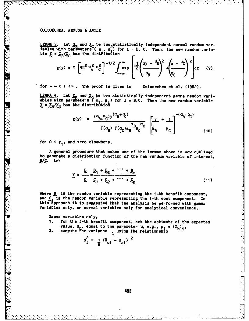
* * . ..
OOICOECHEA, KROUSE & ANTLE
LEMMA 3. Let X andXC be two2statistically independent normal random var-iables with parLeters ( u, o ) for i z B, C. Then, the new random varia-ble Y = IX has the distibuion
g(y) Y [4~O B 1 ex C 2 dz (9)
for - g < Y <m The proof is given in Goicoechea et al. (1982).
LEMMA 4. Let J and X. be two statistically independent gamma random vari-ables with paraketersl ( , Bt) for i : B,C. Then the new random variableY--XB/X has the distribtion
g(y) B+ C%%y' y + 1~ (0
r(%) rcO C O C(0
for 0 < yl, and zero elsewhere.
A general procedure that makes use of the lemmas above is now outlinedto generate a distribution function of the new random variable of interest,a,%. Let
B P, + Z.+ + B
C C + + C (11) _ j A2
where,& is the random variable representing the i-th benefit component,and C Is the random variable representing the i-th cost component. InthisIpproach it is suggested that the analysis be performed with gammavariables only, or normal variables only for analytical convenience.
Gamma variables only,1. for the i-th benefit component, set the estimate of the expected2. value, X , equal to the parameter U, e.g., U - (Xb)i,2. compute he variance using the relationshipII2""2
482.. . . .. .
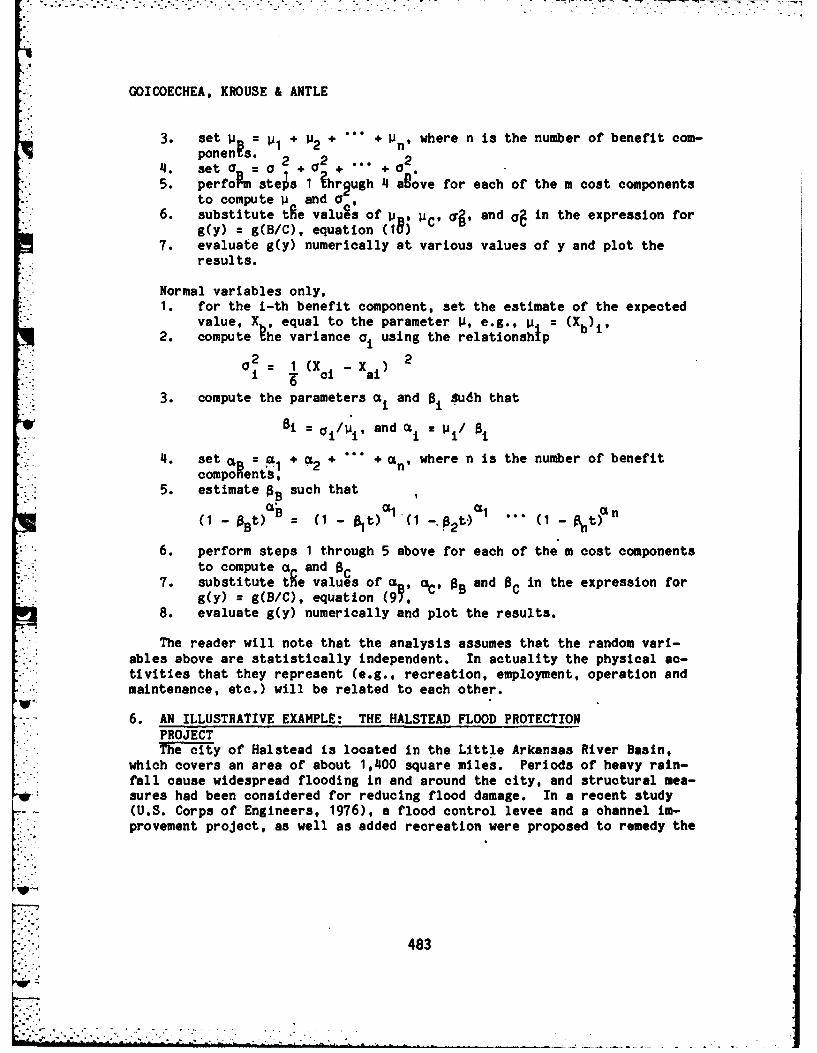
:-
GOICOECHEA, KROUSE & ANTLE
3. set uB = " 112 + + 1 n, where n is the number of benefit com-ponents. 2 2 ... 2
'4. set a = + 02 + + aB 0 1 , +0
5. perform steps 1 hrpugh 4 agove for each of the m cost componentsto compute p and a0 ,
6. substitute tfe values of p, pc, o. , and o in the expression forg(y) = g(B/C), equation (1C) I
7. evaluate g(y) numerically at various values of y and plot theresults.
Normal variables only,1. for the i-th benefit component, set the estimate of the expected
value, Xh, equal to the parameter V, e.g., p = (Xb)i,2. compute he variance a, using the relationship
2 21(X -X xi ci ai
3. compute the parameters at and Sudh that
Bi = :1,'V and a,= 1A1
'4. set +B a + 2 * + an' where n is the number of benefitcomponents,
5. estimate $B such that
-0Bt) I - '(1 -.. B2 t) "' ( - t
6. perform steps 1 through 5 above for each of the m cost componentsto compute a, and SC
7. substitute tfe values of a C, O and Bc in the expression forg(y) = g(B/C), equation (99,
8. evaluate g(y) numerically and plot the results.
The reader will note that the analysis assumes that the random vari-ables above are statistically independent. In actuality the physical ac-tivities that they represent (e.g., recreation, employment, operation andmaintenance, etc.) will be related to each other.
6. AN ILLUSTRATIVE EXAMPLE: THE HALSTEAD FLOOD PROTECTIONPROJECTThe city of Halstead is located in the Little Arkansas River Basin,
which covers an area of about 1,400 square miles. Periods of heavy rain-fall cause widespread flooding in and around the city, and structural mea-sures had been considered for reducing flood damage. In a recent study(U.S. Corps of Engineers, 1976), a flood control levee and a channel im-provement project, as well as added recreation were proposed to remedy the
483
V:.:-
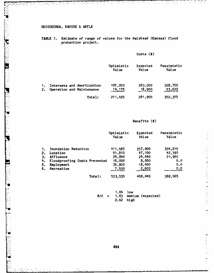
GOICOECHEA, KROUSE & ANTLE
TABLE 1. Estimate of range of values for the Halstead (Kansas) flood
protection project.
Costs ($)
Optimistic Expected PessimisticValue Value Value
1. Interests and Amortization 197,250 263,000 328,7502. Operation and Maintenance 14,175 18,900 23,625
Total: 211,425 281,900 352,375
Benefits ($)
Optimistic Expected PessimisticValue Value Value
1. Inundation Reduction 411,585 357,900 304,2152. Location 51,810 47,100 42,3903. Affluence 26,840 24,440 21,9604. Floodproofing Costs Prevented 16,000 8,000 0.05. Employment 39,800 18,400 0.06. Recreation 7,500 2,600 0.0
Total: 533,535 458,440 368,565
1.04 low
B/C 1.63 medium (expected)2.62 high
484
!,,....,. .... - ... -- - .--- .-- ... .. . . . . . . .. ---. -. b ,
AD-R128 811 PROCEEDINGS OF THE 1982 ARMY SCIENCE CONFERENCE HELD AT 6/6THE UNITED STATES..(U) DEPUTY CHIEF OF STAFF FORRESEARCH DEVELOPMENT AND RCOUISITIO.. iS JUN 82
UNCLASSIFIED F/G 5/2 NLmEMOEENOI
IMhEhEhEMEhhhE
II
11.1 ~~11aa-0 Isl -la
'11.25%4 Lm
MICROCOPY RESOLUTION TEST CHART "ATIom amm tF smoom.gSANATIOMA SIM OF STMOOARDS-1963-A
"1.
MICROCOPY RESOLUTION TEST CHART- -a- -"-.d'~-NATMONLM OFEA orStANOS.163-A - - ---- *
a W-
MiCROemoPY f mhOnNTS HR MICROCOPY RESOLUTI0)I -MST CH*F.,M15U. MM OF 5fMNOjfl5490134 NIO4AI SURIM "NOw*Iinw.a -a
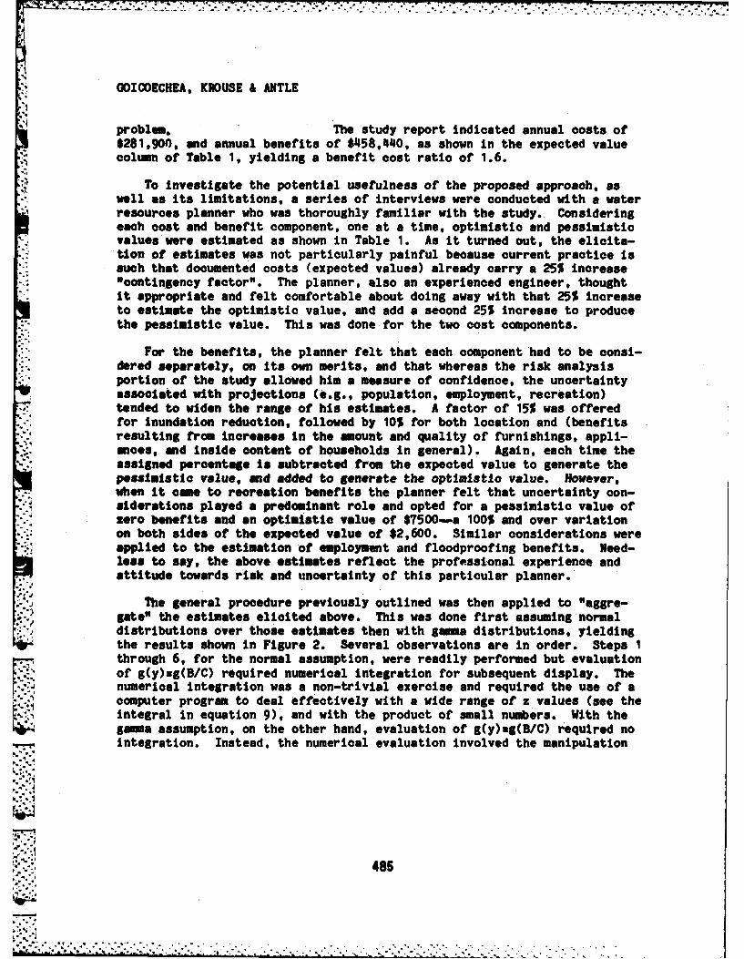
GOICORCHEA, KROUSE & ANTLE
problem. The study report indicated annual costs of$281,900, and annual benefits of $458,440, as shown in the expected valuecolumn of Table 1, yielding a benefit cost ratio of 1.6.
To investigate the potential usefulness of the proposed approach, aswell as its limitations, a series of interviews were conducted with a waterresources planner who was thoroughly familiar with the study. Consideringeach cost and benefit component, one at a time, optimistic and pessimisticvalues were estimated as shown in Table 1. As it turned out, the elicita-tion of estimates was not particularly painful because current practice issuch that documented costs (expected values) already carry a 25% increase*contingency factor". The planner, also an experienced engineer, thoughtit appropriate and felt comfortable about doing away with that 25% increaseto estimate the optimistic value, and add a second 25% increase to producethe pessimistic value. This was done for the two cost components.
For the benefits, the planner felt that each component had to be consi-dered separately, on Its own merits, and that whereas the risk analysisportion of the study allowed him a measure of confidence, the uncertaintyassociated with projections (e.g., population, employment, recreation)tended to widen the range of his estimates. A factor of 15% was offeredfor inundation reduction, followed by 10% for both location and (benefitsresulting from increases in the mount and quality of furnishings, appli-mass, and inside content of households in general). Again, each time theassigned percentage is subtracted from the expected value to generate thepessimistic value, and added to generate the optimistic value. However,when it came to recreation benefits the planner felt that uncertainty con-siderations played a predominant role and opted for a pessimistic value ofzero benefits and an optimistic value of $7500--a 100% and over variationon both sides of the expected value of $2,600. Similar considerations wereapplied to the estimation of employment and floodproofing benefits. Need-less to say, the above estimates reflect the professional experience andattitude towards risk and uncertainty of this particular planner.
The general procedure previously outlined was then applied to "aggre-gate" the estimates elicited above. This was done first assuming normaldistributions over those estimates then with gEme distributions, yieldingthe results shown in Figure 2. Several observations are in order. Steps 1through 6, for the normal assumption, were readily performed but evaluationof g(y):g(B/C) required numerical Integration for subsequent display. Thenumerical integration was a non-trivial exercise and required the use of acomputer program to deal effectively with a wide range of z values (see theIntegral in equation 9), and with the product of small numbers. With thegama assumption, on the other hand, evaluation of g(y)zg(B/C) required nointegration. Instead, the numerical evaluation involved the manipulation
:485
I' - . ..° m •o o
. . .- . •. . . .- . - ". . . . . . . . ...
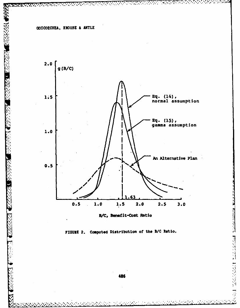
GOICOECHEA, KROUSE & ANTLE
2.0
g (B/C)
1;5 Eq. (14),j normal assumption
Eq. (1.5),gamma assumption
1.0
- An Alternative Plan
0.5
001,/16 _
.50.5 1.0 1 2 02.3.
B/C, Benefit-Cost Ratio
FIGURE 2. Computed Distribution of the B/C Ratio.
46
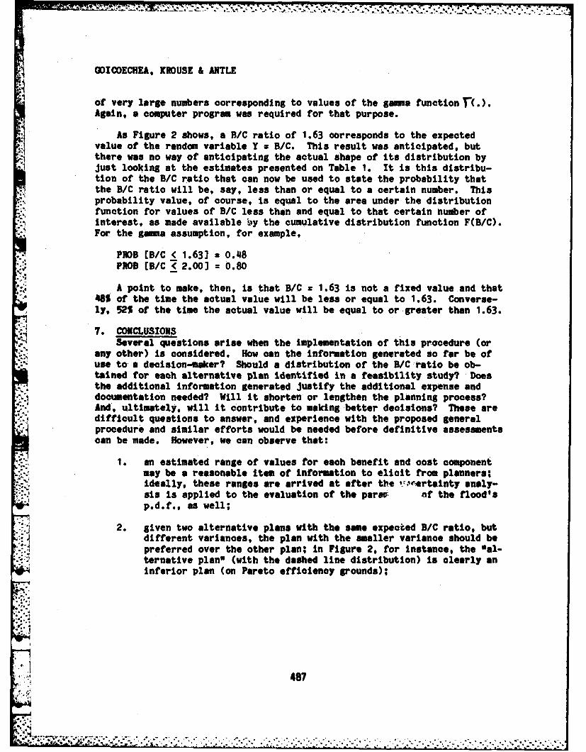
GOICOECHEA, KROUSE & ANTLE
of very large numbers corresponding to values of the gama function r(.).Again, a computer program was required for that purpose.
As Figure 2 shows, a B/C ratio of 1.63 corresponds to the expectedvalue of the random variable Y : B/C. This result was anticipated, butthere was no way of anticipating the actual shape of its distribution byjust looking at the estimates presented on Table 1. It is this distribu-tion of the B/C ratio that can now be used to state the probability thatthe B/C ratio will be, say, less than or equal to a certain number. Thisprobability value, of course, is equal to the area under the distributionfunction for values of B/C less than and equal to that certain number ofinterest, as made available by the cumulative distribution function F(B/C).For the gamma assumption, for example,
PROD (B/C < 1.63J = 0.48PROB (B/C Z 2.00J = 0.80
A point to make, then, Is that B/C x 1.63 is not a fixed value and that485 of the time the actual value will be less or equal to 1.63. Converse-ly, 52% of the time the actual value will be equal to or greater than 1.63.
"1 7. CONCLUSIONSSeveral questions arise when the implementation of this procedure (or
any other) is considered. How can the information generated so far be ofuse toa decision-maker? Should a distribution of the B/C ratio be ob-tained for each alternative plan identified in a feasibility study? Doesthe additional information generated justify the additional expense anddocumentation needed? Will it shorten or lengthen the planning process?And, ultimately, will it contribute to making better decisions? These aredifficult questions to answer, and experience with the proposed generalprocedure and similar efforts would be needed before definitive assessmentscan be made. However, we can observe that:
1. an estimated range of values for each benefit and cost componentmay be a reasonable item of information to elicit from planners;ideally, these ranges are arrived at after the t'prtainty analy-sis is applied to the evaluation of the parau of the flood'sp.d.f., as well;
2. given two alternative plans with the same expected B/C ratio, butdifferent variances, the plan with the smaller variance should bepreferred over the other plan; In Figure 2, for Instance, the "al-ternative plan" (with the dashed line distribution) is clearly an
A inferior plan (on Pareto efficiency grounds);
487
.ti e.-
-:777 a-. -a Z.
GOICOECHEA, KROUSE & ANTLE
3. given two alternative plans with different expected B/C ratio val-ues; but equal B/C ratio variances, the plan with the larger ex-pected B/C ratio value should be preferred over the other plan;
4. for a finite number of alternative plans, each one with a poten-tially different combination of B/C expected value and variance,it is not immediately apparent how to proceed with a ranking andselection of a preferred alternative. The analyst may have to re-sort to multiobjective analysis to explore the tradeoffs (seeGoicoechea et. al., 1982, for a description ofmultiobjective ranking techniques),
5. benefit-oost ratio, or net benefits is not the only criteria forproject evaluation and selection; in fact current procedures callfor the attainment of national economic development (NED), envi-ronmental quality (EQ), social well-being, and regional economicdevelopment objectives; the needs exist, it would appear, to con-sider benefit-cost analysis within a multiobjective framework; inthat framework, the B/C expected value and variance represent use-ful information in a list of criteria to use to evaluate and rankalternative plans.
6. the matter of arriving at estimates of the ranges appropriate forthe various components of benefit and cost, can be difficult attimes and can very from one planner (e.g., decision-maker) toanother; by necessity, these estimates are of a subjective natureand reflect whether a planner is risk-averse, risk-prone, or risk-neutral; however, once the estimates are arrived at, the analyti-cal procedure developed can be applied to aggregate the effects ofparameter variation and produce a probability distribution of theB/C ratio.
REFERENCES
- Goicoechee, A., D. R. Hansen, and L. Duckstein, Multi-ObjectiveDecision Analysis with Engineering and Business Applications, to bepublished by John Wiley and sons in 1982, 640 pp.
- U.S. Corps of Engineers, "Survey Report for Halstead Local FloodProtection Project," Feasibilitt Report, September 1976.
- U.S. Water Resources Council, Procedures for Evaluation of National
Economic Development (NED) Benefits and Costs in Water ResourcesPlanning (Level C), Federal Register, Vol. 54, no. 102, pg.30194-30258, Washington, DC, May 24, 1979.
.488
488
............................
GOICOECHEA & KROUSE
A COMPUTER-BASED INTERACTIVE MODELFOR INDUSTRIAL LAND USE FORECASTING
AMBROSE GOICOECHEA, Ph.D.International Water Resources Institute
School of Engineering andApplied Sciences
George Washington UniversityWashington, DC
MICHAEL R. KROUSEInstitute for Water ResourcesU. S. Army Corps of Engineers
Fort Belvoir, Virginia
1.* INTRODUCTIONAn industrial engineering activity that is growing in relevance and
receiving due attention in the literature is that of identifying land areassuitable for future industrial use. As cities expand and multiply, thevarious activities that reflect the social-economic makeup of a community(e.g., industrial, commercial, residential, agricultural, etc.) competewith each other for use of the same fixed resource-land. It then becomesnecessary and meaningful to consider the science and art (e.g., economicand behavioral aspects) of land use forecasting.
Land use forecasting has long been a planning activity of interest to-._4 the various Federal and State agencies, particularly those with mandates
for the development of land and water projects. Certainly this is the caseat the U.S. Army Corps of Engineers, where land use forecasting has longbeen applied to the evaluation of economic benefits resulting from engi-neering measures and associated land uses. Over the last 50 years a number
of research efforts have been funded by the Corps relating to the develop-ment of analytical land use methodologies and, in some cases, the design ofcomputer-based forecasting models.
The purpose of this paper, then, is to review briefly the progress1made in the analytical and behavioral development of land use forecasting
models, to point to the modeling functions of special relevance to
Np
489.1
'.- .:.:', . .. .." . .. . . j .. ' ...... ' . . - - .. .. . . . .. . . . . . . . . . . .- . .. .
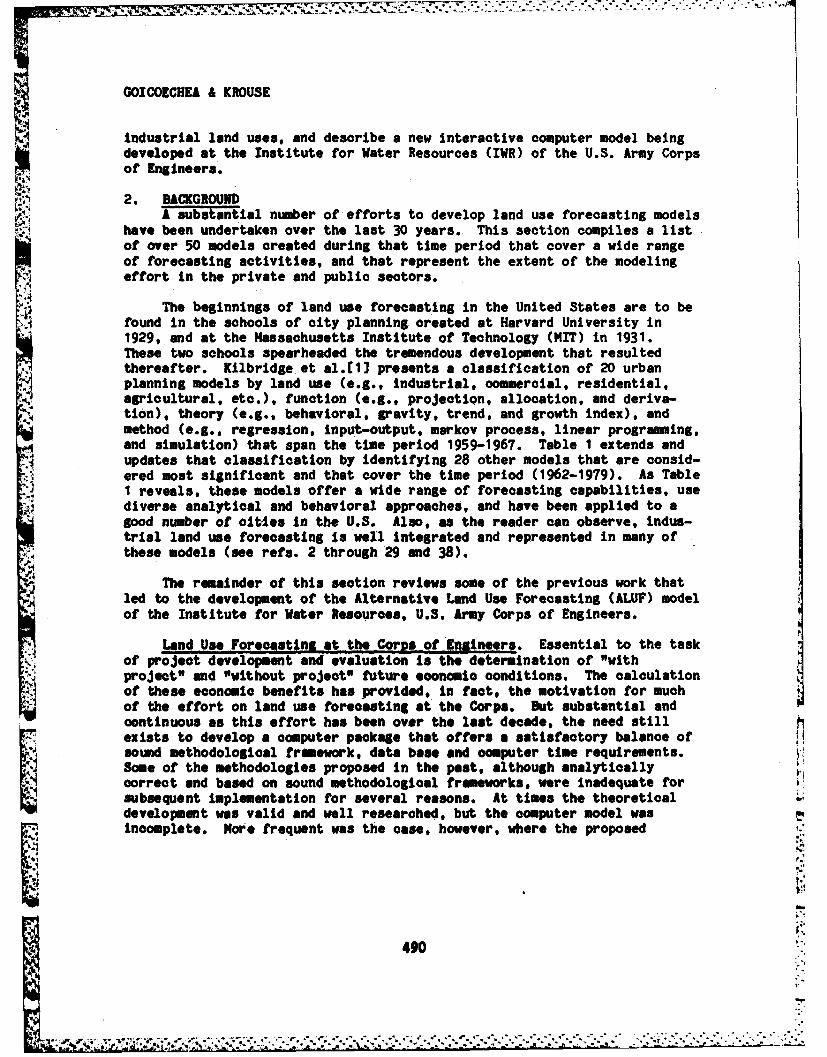
GOICOECHEA & KROUSE
industrial land uses, and describe a new interactive computer model beingdeveloped at the Institute for Water Resources (IWR) of the U.S. Army Corpsof Engineers.
A substantial number of efforts to develop land use forecasting modelshave been undertaken over the last 30 years. This section compiles a listof over 50 models created during that time period that cover a wide rangeof forecasting activities, and that represent the extent of the modelingI! effort in the private and public sectors.
The beginnings of land use forecasting In the United States are to befound in the schools of city planning created at Harvard University in1929, and at the Massachusetts Institute of Technology (MIT) in 1931.These two schools spearheaded the tremendous development that resultedthereafter. Kilbridge et sl.[1] presents a classification of 20 urbanplanning models by land use (e.g., industrial, commercial, residential,agricultural, etc.), function (e.g., projection, allocation, and deriva-tion), theory (e.g., behavioral, gravity, trend, and growth index), andmethod (e.g., regression, input-output, markov process, linear programming,and simulation) that span the time period 1959-1967. Table 1 extends andupdates that classification by identifying 28 other models that are consid-ered most significant and that cover the time period (1962-1979). As Table1 reveals, these models offer a wide range of forecasting capabilities, usediverse analytical and behavioral approaches, and have been applied to agood number of oities in the U.S. Also, as the reader can observe, indus-trial land use forecasting is well integrated and represented in many ofthese models (see refa. 2 through 29 and 38).
The remainder of this section reviews some of the previous work thatled to the development of the Alternative Land Use Forecasting (ALUF) modelof the Institute for Water Resources, U.S. Army Corps of Engineers.
Land Use Forecasting at the Corps of Engineers. Essential to the taskof project development and evaluation is the determination of "withproject" and "without project" future eoonomli conditions. The calculationof these economic benefits has provided, in fact, the motivation for much
* of the effort on land use forecasting at the Corps. But substantial andcontinuous as this effort has been over the last decade, the need stillexists to develop a computer package that offers a satisfactory balance ofsound methodological framework, data base and computer time requirements.Some of the methodologies proposed in the past, although analyticallycorrect and based on sound methodological frameworks, were Inadequate forsubsequent implementation for several reasons. At times the theoreticaldevelopment was valid and well researched, but the computer model wasIncomplete. MoOe frequent was the case, however, where the proposed
490
7 7:
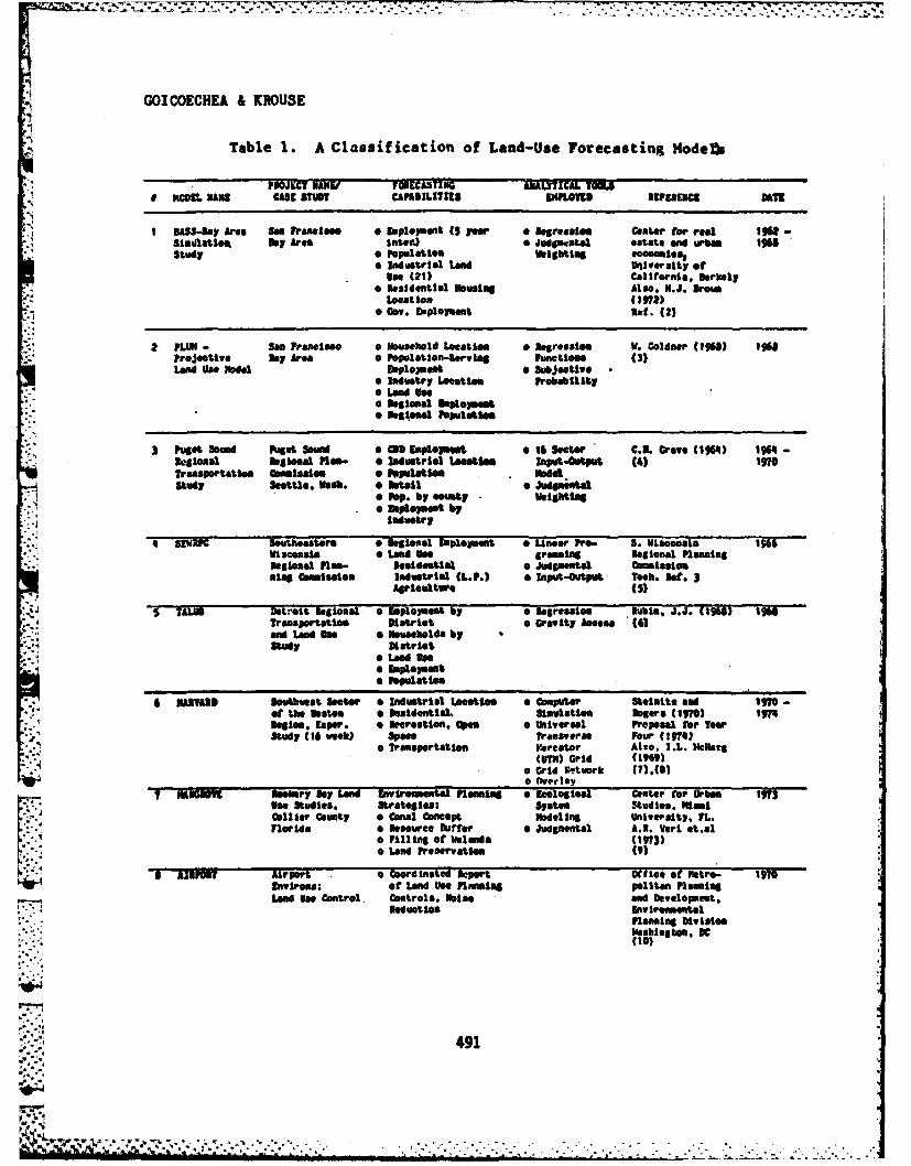
GGICOECHEA & KROUSE
Table 1. A Classification of Land-Use Forecasting Models
PIUOJCT ANU F-- ECASTING AALYTICAL TOM S
# mo0hEL MANE CASE SiUmI CAPABILIMTXS DPMTEn I muenImJcg DAY9
I uSUS-av Area Sa franeiaoo * Iplaepnt (5 Year * Uereealaa Center top real Ion -.Sialatlo y Da Area lnter) a Juddaintal eatate and Jwbam I05Study * population Vaightiq eoobmi5e
a lndutrial Land tjivewrsity ofuse (21) Caltornia, lerkely
* aesidential buslng Alao. N.J. romLocation (72)
0 * Gov. bploytent at. (2)
2 MAUN -Sam Promises a Household Locat.ion o loreslon V. Goldner ( 0
2. n rojective Bay Area 0 Population-Uervwin Functions (3)Land Use NWe4 Eploe m a SuJeetio •
* Industry Locatto ProbabflitySLad Use
*• Ne~seal Fopulaotes
3 puet Sound Fug"t nd a Coa Ioplemt 0 16 sector C.N. Grave (190) 11 -
Regional Dienoal Plan- 0 bdustrial Le tieoe Input-Outkpt (4) 1970Transportatioe Comisii a Populatie odStudy Seattle. Wak. o Motail 0 Judgumla
. Fop. by emty eishti- Eploe ot by
Industry
• SENIC 5uO beaaters • logional nlmo~uet o Linear Pro- 3. Wisconsin 1566Visconsin o Land hi grm ala Declonal PlmnningUeg aaSl Plan- Residential • Judgmentel camilsolosing Comisalam Industrial (L.P.) a Input-Output Teab. let. 3
Arieultuo (5)
S TAlS Detroit Regional 0 mplo ent by a Regressioa pubis, J.3. (108) 16Transportatlee Dstrict 0 Gravity A"es" (6)snd Lead UN a Nuaeholds byStudy DIstrict
* Load Uh
Fopu atioa
6 11"VMAS fsuthuwa Seter 0 Industriel Looseti • Computer Steimtte mmd IND -at the ts$m a Masidentihl, Sinulatem oSers (IwO) 19""51iam, gaper. a Wsrestion. Open a Universal Proposal Mor lewStudy (IS Week) Spaee fransvema Four (1974)
* Trnnsportation Fercator Also, I.L. PesaroMTIM) Grid (1909)
aGrid Networke M()SI~ qr•overlay
MUMU9E tookery Bey Lad 9nvIro.mental PIming 0 [aloolol Center for Urban 1973use Studies. strategies: System S0tudis. HimilCollier county a Canal Concept odelIng University. FL.Florida a Resource Surfer o Judgmental A.%. Vetrl t.al
0 Filling of lelond (1973)* Land Preservatioe (9
I AISPURT Airport 0 Coordinated Rkport Office ofMitro- 1970Environ: o Land Use lannnl polltan PIlMingLead Use Control ContrOl$. Poise and Develolpet,
Reduotliom Envirometalplanning Diviaion
491ntn O
'.o" 491
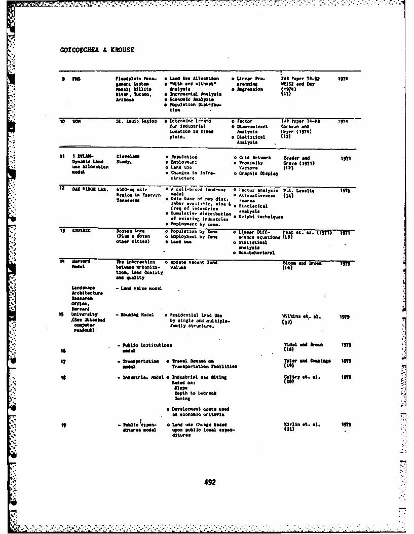
.....................................
GOICOECHEA & KROUSE
n9 1 Floodplain mana- o Land Use Allocation o Linear Pro- IWR Paper 74-82 1974gement System * "With and wlthout greming WEISZ and DayHdel; Rillito Analysis Regreasion (1974)lver. Tucsono. Increentsal Analysis (11)
Arizona o Economic Analyaaio Population DiaLribu.
tion
10 UtR St. Louis hegion o Za.termine Ltvvzd o Factor IWO Paiper 74-Ps 197sfur industrial 0 Dis.riminant Corbean andlocation In flood Analysis Fryer (1974)plain. • StatiatIcal (12)
Analysis
11 1 DLAN- Cleveland o Population 0 Grid Network Saader aOd |7Dynamic Lend Study. o eAplopavn? O Proximity Crave (1971)s allocation a land use Factora (13)
model o ChanSCs in Infra- 0 Graphic DisplayLructure
12 OAK VIDGE LAS. 6500-eq mile 0 A cell-. ,! land-use 0 Factor enalysie l.A. Leseiae 1976Region in .estern model 0 Attractiveness (1)Tennessee o Data bane of pop dist, scores
labor availible. size 4 o statistical[req of infi.asrie ao Cumulative distribution analyaleof existinc induscries o Delphi techniques
o Employment by zone.
13 ENPIRIC Boston Ares o Population by Zone o Linear Ditt- Peat St. si. (1971) 197.(Plus a dozen o Employment by Zone eoence equations (15)other cities) o Land use o Statiatical
analysisa Non-behavioral
14 Marvad The interaction o update vacant lnd Bloom and broue 197Hodel between urbaniza- values (16)
tios. Land ualityand quality
Landscape - Land value modelArchitetreResearchOfflo, oHarvard
15 University - ousing Model o esidential Land Use Wilkina et. &1. 1979- .Sea, Att ahd by single a nd multiple. (17) .'T,' computer- fa.mily structure..'- readout) -
:;,- publio institutions Vidal and brown 19"f
6 .model
1T - Transportation o Travel Demand on Tyler and Coaleuga 1N97moel Transportation Faoillties (19)
"I -IndutriA& Model a Industrial use siting (°1B0) e. *I. if"Based on:slopeDepth to bedrockZoning
o Development costa ugeas economic criteria -
19 - Public 'epn- o Land use Monge based Kirlin st. al. 1t"% turee model upon public local expen- (21) *.
dilutes
-C
492
C.~ 4I~L42~~ ~~.L4 -
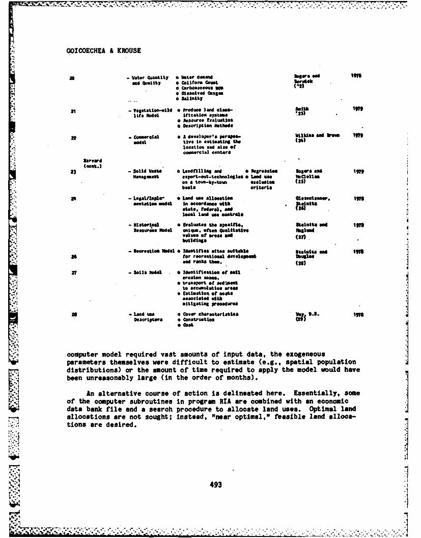
GOICOECHEA & KROUSE
so - water Quantity o water demand logers a"6 19fand Quality o Coliform Cout eriok
0 Carbonaceous aO (42)
o Dissolved Oxygen0 Salnlalt
21 .Vegitstion-ld o Froduce land class- Smith 1119life Yodel iflcatilo systems !,)
R esource Evaluation* Description Heathoda
22 - Commercial 0 A developer's perspoe- Wilkins and br 1omdel tv* in estimating the (2.)
locatior and size ofcoemerctal centers
Narvard(cant.)
23 - Solid waste o Landfilling and Regressing Rogers am 119Managment *sport-out-teehnologies • Land ws Hlellsm
on a town-by-ton eacluslon (25)besis criteria
"4 - Legal/lople, o Land use allocation Glezentamer. 1mnatioa model In accordance with . Reit:
state. federal. .and (26)local land use controls
- Historieal e Evaluates the spelfico Stelmtz and 11r8Resources rodel unique. often Qualitative 1aliad
values of areas and (f).buildings
- 26ecretiom Nodel o Identifin Sites SUital 8teaiita 11826 for recreational development bugus
and ranks them. (28)
27 - Soils del 0 identifieation of solerosion znnes.
o transport of sedimentto accumulation areas
o Etlaation of costsassociated withmit igating procedures
2 - Land we o Cover characteristics Is D.S.De rptors o Construction
o cost
parameters themselves were difficult to estimate (e.g., spatial population
distributions) or the amount of time required to apply the model would havebeen unreasonably large (in the order of months).
An alternative course of action is delineated here. Essentially, someof the computer subroutines in program RIA are combined with an economic
1data bank file and a search procedure to allocate land uses. Optimal landallocations are not sought; instead. "near optimal," feasible land alloca-tions are desired.
-%.. 493

001 COECHIA & IROSE
3. ALTEBJATIVE hAID USE FoREcASTINQ (ALUF) PGRANThe devel s~t of a grid cell data file requires that each variable
MaP be Individually encoded and geographically registered to a common baseand stored. along with data variables In the data bank, on a computer stor-Age device.
The IWR package consists of two computer programs which are used inconnection with a grid cell spatial data base as shown In Pigure 1. TheTaipegam terntie and U Forecasting (ALUF) does the actualallocna tion of futuretlnd uses to spesific grid calls. The Existing LandUse Analysis Program (ELUA) is provided to help identify significant land4 use location factors for the allocation process based on the relationshipbetween laad use locations and other, dat available in the grid cell databank.
The final progrm output is a new data variable written into the database file for each grid cell, Indioatin- projected future land use. Theprograms are written In FORTRAN IV for the GDC 6600/7600 series computers.
The . AWprogram incorporates th-eHEZ IA Attractiveness modelingprogram and R1. Distance Deteaiftion package. These were adapted for usein this process so that land use locator sores can be developed accordingto user specified criteria, as ell ,as location criteria derived from thestatistical findings.
The kinds of data variables mbnly used as a basis for allocating
future land use include:
A. Access (Distance)
I. Transpiortation2. Central Business Districts or Regional Centers3. hependent ko'tivttes
B. Proximity to Compatible Land UsesC. Physical Land Attributes (Developability)
1. Slope2. Drainage
3. Typ or Cover,LI. Sells
V. Infrustruotut~r1. Sewers and Water2. Gas and Powe3. Mess Tr antt
9 . Zon-ing,. oweraip
. Lmd Mrioe
4,4
N$
4 -4 A .,- "'.- !,.
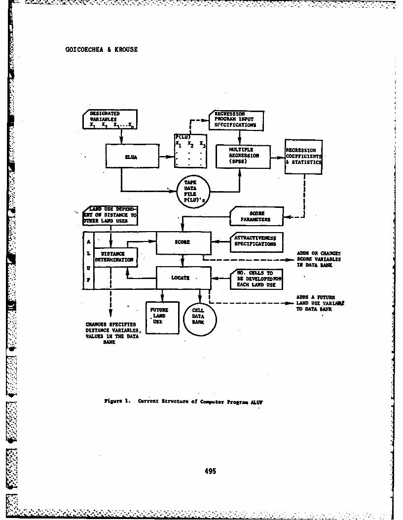
GOICOECHEA & KROUSE
DESEIRESSEONREGRESSCON
VARIABLES----------~ PROGRA INPIBUT
X1AE SPECPECFFIAION
VALUES. 13Th3DT
- DATA
-. FUZP..U).
O-M SE4E
DLuE 1 urn SrcueofC. o PormAU
DISTACE TO S495
PARAMETER
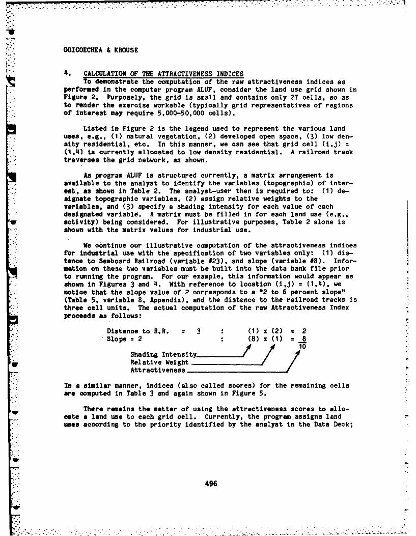
GOICOECHEA & KROUSE
4. CALCULATION OF THE ATTRACTIVENESS INDICESTo demonstrate the computation of the raw attractiveness indices as
performed in the computer program ALUF, consider the land use grid shown inFigure 2. Purposely, the grid is small and contains only 27 cells, so as
... to render the exercise workable (typically grid representatives of regionsof interest may require 5,000-50,000 cells).
Listed in Figure 2 is the legend used to represent the various landuses, e.g., (1) natural vegetation, (2) developed open space, (3) low den-sity residential, etc. In this manner, we can see that grid cell (ij)(1,4) is currently allocated to low density residential. A railroad tracktraverses the grid network, as shown.
As program ALUF is structured currently, a matrix arrangement isavailable to the analyst to identify the variables (topographic) of inter-eat, as shown in Table 2. The analyst-user then is required to: (1) de-signate topographic variables, (2) assign relative weights to thevariables, and (3) specify a shading intensity for each value of eachdesignated variable. A matrix must be filled in for each land use (e.g.,activity), being considered. For illustrative purposes, Table 2 alone isshown with the matrix values for industrial use.
We continue our illustrative computation of the attractiveness indicesfor industrial use with the specification of two variables only: (1) dis-tance to Seaboard Railroad (variable #23), and slope (variable #8). Infor-mation on these two variables must be built into the data bank file priorto running the program. For our example, this information would appear asshown in Figures 3 and 4. With reference to location (ij) (1,1), wenotice that the slope value of 2 corresponds to a "2 to 6 percent slope"(Table 5, variable 8, Appendix), and the distance to the railroad tracks isthree cell units. The actual computation of the raw Attractiveness Indexproceeds as follows:
Distance to R.R. 3 (1) x -2 2Slope z 2 (8) x ( ) 8
Shading Intensityv Relative Weight
Attractiveness
In a similar manner, indices (also called scores) for the remaining cellsare computed in Table 3 and again shown in Figure 5.
There remains the matter of using the attractiveness scores to allo-cate a land use to each grid cell. Currently, the program assigns landuses according to the priority identified by the analyst in the Data Deck;
496. . . . . .... ..-
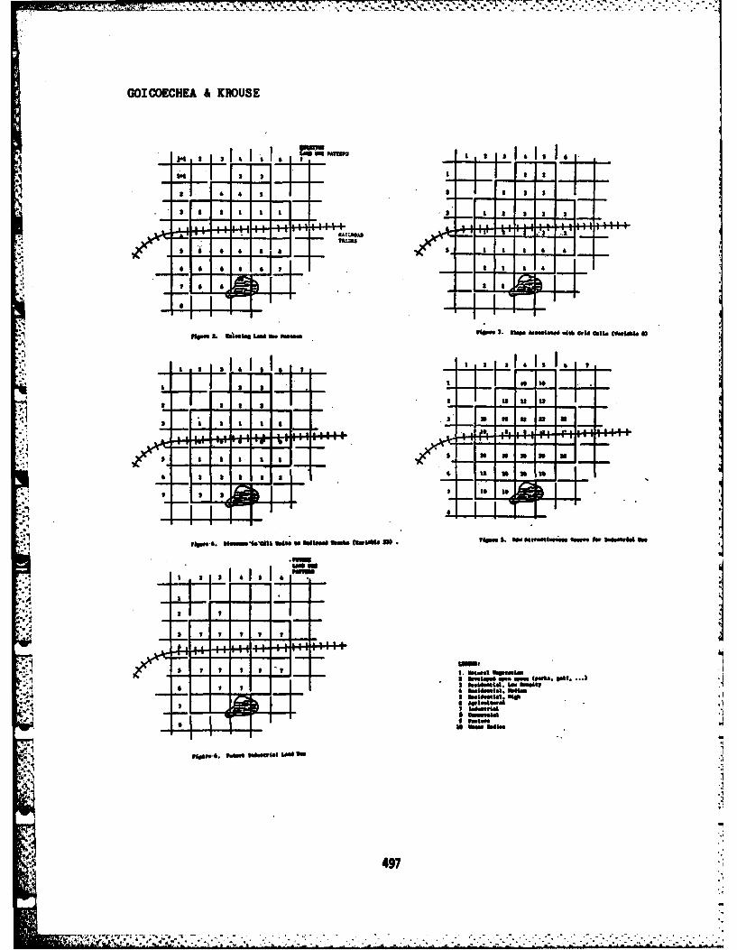
GOICOECHEA & KROUSE
a 3 &~I II I.I
is
n - 0 a n I
4- ++
a a 1 3 a 39 36 -0
of a
4-444-14-4117Hem ~ ~ ~ ~ ~ ~ p fI." "a*~beb t. bdbl ~ei
a a.II I a isle i
a aft"4 a o V I 0
a _ _ a a a asa49i
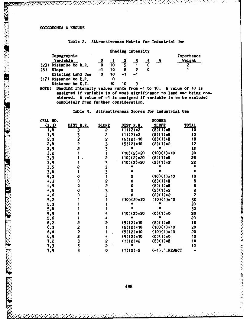
GOICOECHEA & KROUSE
Table 2. Attractiveness Matrix for Industrial Use
Shading IntensityTopographic ImportanceVariable 0 1 2 3 4 5 Weight
(23) Distance to R.R. -0 - 5 -1 0 2(8) Slope -1 10 8 2 0 1
Existing Land Use 0 10 -1 -1(17) Distance to E.R. 0
Distance to E.I. 10 10 9NOTE: Shading Intensity values range from -1 to 10. A value of 10 is
Ki assigned if variable is of most significance to land use being con-sidered. A value of -1 is assigned if variable is to be excludedcompletely from further Consideration.
Table 3. Attractiveness Scores for Industrial Use
CELL NO. SCORES(ij) DIST R.R. SLOPE DIST R.R. SLOPE TOTAL1,4 3 (1)(2)2 TF71w8 101,5 3 2 (1)(2)=2 (8)(1)28 102,3 2 2 (5)(2)=10 (8)(1)w8 182,41 2 3 (5)(2)=10 (2)(1)a2 122,5 2 3 123,2 1 1 (10)(2)=20 (10)(1)z1O 303.3 1 .2 (10)(2)z20 (8)(I)=8 283,4 1 3 (10)(2)=20 (2(1)=2 223,5 2 3"3,6 1 34,2 0 1 0 (10)(1)210 104.3 0 2 0 (8)(1)=8 84,4 0 2 0 (8)(1)=8 84,5 0 3 0 (2)(1)=2 24,6 0 3 0 (2)(1)=2 25.2 1 1 (10)(2)=20 (10)(1)=10 305,3 1 1 3 305,4 1 1 305,5 1 4 (110)(2)z20 (0)(1)=0 20
5,6 1 34 206,2 2 2 (5)(2)=10 (8)(1)V8 186,3 2 1 (5)(2)110 (10)(1)Z10 206,4 2 1 (5)(2)=10 (10)(1)210 206,5 2 4 (5)(2)=10 (0)(1)sO 107,2 3 2 (1)(2)z2 (8)(1)18 107.3 3 2 " 107,34 3 0 (1)(2)=2 (-1).".REJECT -
t.°4
': 498 '
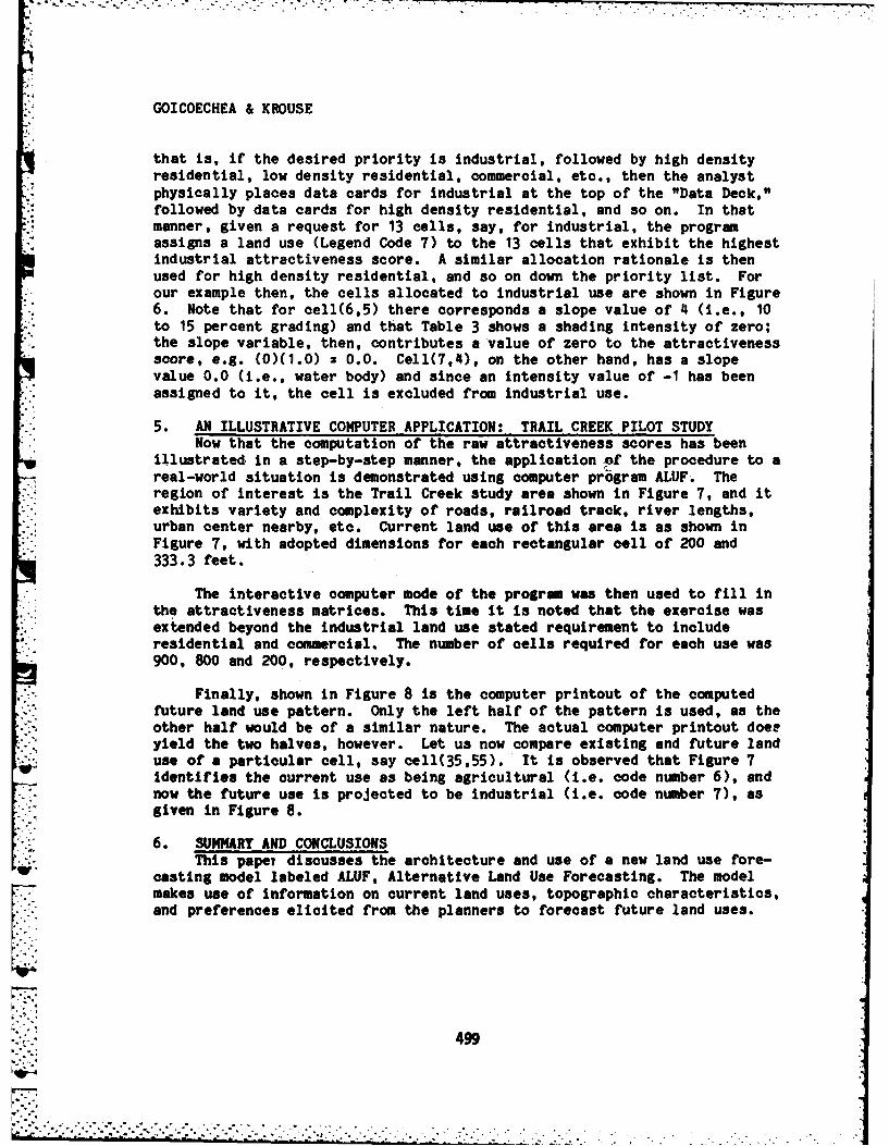
GOICOECHEA & KROUSE
that is, if the desired priority is industrial, followed by high densityresidential, low density residential, commercial, etc., then the analystphysically places data cards for industrial at the top of the "Data Deck,"followed by data cards for high density residential, and so on. In thatmanner, given a request for 13 cells, say, for industrial, the programassigns a land use (Legend Code 7) to the 13 cells that exhibit the highestindustrial attractiveness score. A similar allocation rationale is thenused for high density residential, and so on down the priority list. Forour example then, the cells allocated to industrial use are shown in Figure6. Note that for cell(6,5) there corresponds a slope value of 4 (i.e., 10to 15 percent grading) and that Table 3 shows a shading intensity of zero;the slope variable, then, contributes a value of zero to the attractivenessscore, e.g. (0)(1.0) = 0.0. Cell(7,4), on the other hand, has a slopevalue 0.0 (i.e., water body) and since an intensity value of -1 has beenassigned to it, the cell is excluded from industrial use.
5. AN ILLUSTRATIVE COMPUTER APPLICATION: TRAIL CREEK PILOT STUDYNow that the computation of the raw attractiveness scores has been
illustrated in a step-by-step manner, the application of the procedure to areal-world situation is demonstrated using computer program ALUF. Theregion of interest is the Trail Creek study area shown in Figure 7, and itexhibits variety and complexity of roads, railroad track, river lengths,urban center nearby, etc. Current land use of this area is as shown inFigure 7, with adopted dimensions for each rectangular cell of 200 and333.3 feet.
The interactive computer mode of the program was then used to fill inthe attractiveness matrices. This time it is noted that the exercise wasextended beyond the industrial land use stated requirement to includeresidential and commercial. The number of cells required for each use was900, 800 and 200, respectively.
Finally, shown in Figure 8 is the computer printout of the computedfuture land use pattern. Only the left half of the pattern is used, as theother half would be of a similar nature. The actual computer printout doeryield the two halves, however. Let us now compare existing and future landuse of a particular cell, say eell(35,55). It is observed that Figure 7Identifies the current use as being agricultural (i.e. code number 6), andnow the future use is projected to be industrial (i.e. code number 7), asgiven in Figure 8.
6. SUMMARY AND CONCLUSIONSThis paper discusses the architecture and use of a new land use fore-
casting model labeled ALUF, Alternative Land Use Forecasting. The modelmakes use of information on current land uses, topographic characteristics,and preferences elicited from the planners to forecast future land uses.
499
> . . . . .. -
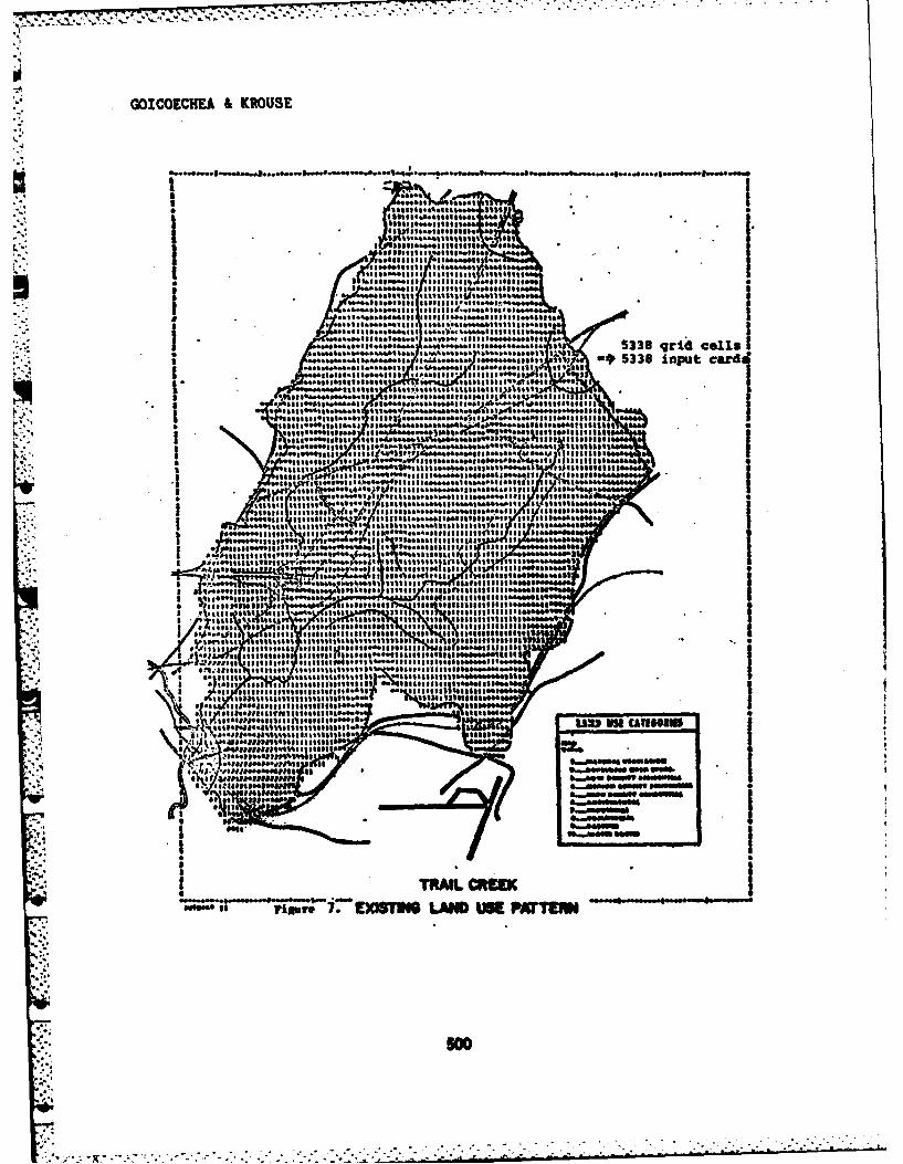
GOICIOECHEA It KROUSE
is l ook.,es.. .. .I
o# I Oto6 601a J....i.66--60tosI tue~u 6lbegige~
* ..,I~..... ...g 5338II..b...aggcellsiglI
................... e..94 mom.oaees
1 000101 1 ... 4 lot... 5& OS*fI ~ i
to wboam is ti u o
iesl t =1641 too~ ti.a$$O 0,0-0641!-61 its ,..::N ...ssiiia~ua
6%"611S~a114,"60-60 los*t I I I i...k"
1.iti %a $1..*~ 11iii~S&~liIi~p~ ... *ti*S99&a..!S,99''...4.mis .. , is 1 11 M=,
$*sti4t446 i illtl~ll "4 .I r ls
.6.i1e 1 ,mIfih 9't% ., Mo b" IIILI it 15 to ::Ia64
* ~ ~ ~ ~ ~ 16 eas l * , ,smsiIsiIm . It 11S.IsS*I 16S0 I
0, - I = 6 11,ttlttt 11 Mosmiitll.e~ae t~
*i4~.Ltt*#e~~lt 9ilttiii lestsea I@% ISISI -,.ff a -^- m stIill I
*,.l. .me .aI I'll " 1
to's .", MNMM -0. -
91. I'saa Z-4M 669161096
a o
I I11 i As
6: a @"now"
T IUhID -
*4ix;~~m j0 XW AWUE lM
So
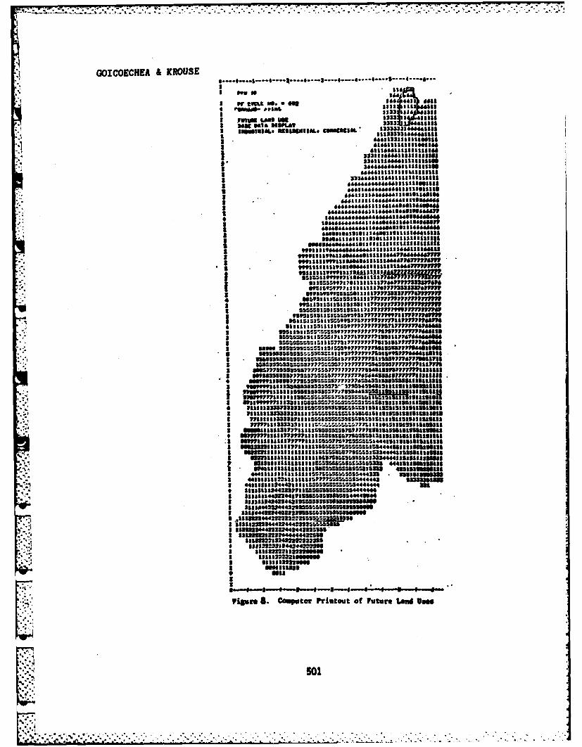
GOICOECHEA & KROUSE
36 6
51334 11 all,31
* uuassuasuu 222
I =wstg 3 3*0mlY22 "&$IS$
323*66616 12:o6466=a tS s 6S I o si 03 036056664**43 $~6316m11 sa48 6*SIIIS6UISII ao*6,1111116631
I ,,,Sl~~l9~6~SA4 66 688153S1S1'6
is 323iamaa 66111a6d'slss l111I ~ ~ ~ ~ ~ -! ,, 1 3 1 a,~~'*~aaIIasn
2~~~~~~ a"ii64,88 a 31l3211fl67fl12PI iii~gisssa ii 4637636161 1111141666W
3 3*, 31313.113 6 i19Sf71P7V 112PMPP.6** ~ ~ ~ ~ 1= 43ii3ii~959l77fh~1611766I Sli Iii i~~.iii4if667?64 7129619P12634
3 . 21i552i5511~lillliZ17 117 v a"~l771 S1,3"0
* US9I9IU~hSP17U51i5777717S777ii~1UPlSI.SI.
$U 1 1& 1243233553535 2711SUl5 11111 S M sasSNISS
3 1147733333231SMSUSS71I'~ 52i5S11I
17* I~f l 133331171 as i5i75i11 I IM 11148351 11112
3t 11l33333l331115i7Si124448112I555a313553
F 11331333132 13513 165V.511333 4441aSSSSsll
3 4333333444331 a 576=5~t 1444,43 fl33iM
3 1i122212 35.1i5t55522l
3 3344 2443511 ?btiaISlISWI 3344234432sm11lU~il.S
was1
3Cmpa Prntu of Future Land VowIiS2I
3 3 3I344I23543411

GOICOECHEA & KROUSE
In the process, It calculates the economic benefits to be derived from aproposed engineering measure or zoning policy. The model is currentlyoperational and it is available to Corps personnel and general city plan-ners involved In project development and evaluation. Also, it is hopedthat industrial engineering practitioners will find it useful in theirdialogue with city planners as new Industrial enterprises in growing commu-nities are discussed.
REFERENCES
Kilbridge, M., R. O'Block, and P. Teplitz, "A Conceptual Frameworkfor Urban Planning Models," Management Science, Vol. 15, No. 6, 1969.
Brown, H. C., J. R. Ginn, F. J. James, J. F. Kain, and M. R.Straszheim, Empirioal Models of Urban Land Use: Suggestions onResearch Objectives and Organization, Exploratory Report 6, NationalBureau of Economic Research, New York, 1972.
Goldner, W., Projective Land Use Model (PLUM), Bay AreaTransportation Study Commission, BATSC Technical Report 219, SanFrancisco, California, September 1968.
Hydrologic Engineering Center, Resource Information and AnalysisUsing Grid Cell Data Banks. Computer Program 4D1-X6-L7590; UserManual, U.S. Army Corps of Engineers, Davis, California, September
Hydrologic Engineering Center, An Investigation of Concepts andMethods for Broadened Scope Flood Plain Information Studies, PhaseI . Oconee Basin Pilot Study, U.S. Army Corps of Engineers, Davis,California, September 1975.
Jolissaint, C. H., Issues Related to Interfacing Water ResourcePlanning and Land Use Planning: Development and Application ofQuantitative Proodures, INTASA, Inc., Menlo Park, California, May1977.
Note - Space limitations preclude a .complete listing of references.Please write to authors requesting such listing.
.40
. . . . . . -' . . . .. - .. . ., . . -. .. -. ,
4 . . . . . . . . . . . . . . . . . . . . . . . . ....... . .... . . . . . . . . . ... 7.-,7 7. ..
GOLDMAN
MICROCLIMATE COOLING FOR COMBAT VEHICLE CREWMEN (U)
RALPH F. GOLDMAN, Ph.D. and STAFFU.S. ARMY RESEARCH INSTITUTE OF ENVIRONMENTAL MEDICINE
NATICK, MA 01760
1. INTRODUCTION
At air temperatures above 25°C ($20 F), human thermal comfort is bestachieved without clothing; however, it m be essential if the human is exposed tocontact with surfaces above 45 C (113 F), sunlight, blowing sand, drying wind,missiles and/or NBC agents. Increasing protection is associated with increasingthickness of barrier layers on the skin. Unfortunately, any barriers between the skinand the ambient environment reduce the ability to eliminate heat from the body.
a) BODY HEAT PRODUCTION
Heat production (M) at rest is about 1 Met (50 kcal of per square meter ofbody surface area per hour); an average man's heat production at rest is 90 kcal/hror 105 watts. Normal work can double heat production and hard work can triple it.The sustainable "voluntary hard work" level is w5 Met (425 kcal/hr or 500 watts),while 6 or 7 Met will exhaust the average man if sustained for a few hours.
b) BODY HEAT LOSS MECHANISMSAbout 12% of the resting heat production is eliminated from the lungs by
respiration. Another 12% is eliminated by evaporation of the body water diffusingthrough the skin; up to 0.6 kcal of heat is removed for each gram of water
-"i evaporated. Evaporation can, however, be blocked by ambient vapor pressuresgreater than the vapor pressure of water at skin temperature or by clothing which,even if permeable to water vapor, reduces the potential evaporative cooling byimposing insulation between the skin and the environment. The remaining 76% ofresting metabolic heat production is eliminated from the body by convection andradiation in a comfortable environment. Elimination of the increased heatproduction during work s facilitated by the convective air motion generated by body"pumping", but in a warm environment most of the increased heat production is lostby production of sweat and its subsequent evaporation; even in a cold environment,about 42% of working heat production may be lost by evaporation.
~I.
503
...... ................... .I
", ''a- -:~a k ,,= -_ _ , +: ., " . S. . --.. . .. S .- -...
GOLDMAN
c) STILL AIR INSULATION; THE "CLO" UNITEven without clothing, there is a barrier layer of still air next to the skin.
This still air film acts as insulation against heat exchange between the skin and theambient environment; without body or air motion this external air layer (1a) provides0.9 cl4 of insulation. One clo unit of clothing insulation is defined as allowing 5.55
kcal/m /hr of heat exchange by radiation and convection (H:RC) for each C oftemperature difference between the skin (at average skin tenperature Is) andambient air temperature (Ta). Since the average man has 1.8 m of surface area,his H:RC can be estimated as: H:RC = (10/clo) (Ts - Ta) EEq. 13; i.e. an 0.8 clo stillair layer limits the heat exchange by rafiation and convection for a nude man toabout 12.5 kcal/hr (10/0.8) for each C of difference between skin and airtemperature. Thus, producing 90 kcal/hr, a resting man will lose I I kcal/hr (12%) byrespiration, 11 kcal (12%) by evaporation of the water diffusing through his skin andwill have a requirement to evaporate sweat (Ereq) to eliminate the remaining68 kcal/hr if the Ta is less than 5.5C (i.e. 68/12.5 kcal/hr/0 C) below Is. Therequired sweat evaporative cooling (Ereq) can be estimated as: Ereq = M + (H:RC)L Eq. 23 where M is the heatproduced during rest or work and H:RC is estimated byEq. I. Since a comfortable Ts is about 330 C (91.4°F), an increasing percentage ofthe body surface area will be required to be sweating with a Ta above 27.5 0C (i.e.33 -53)
The external air layer is reduced by air motion, approaching a minimal valueof*vO.2 co at air speeds above 4.5 m/s (10 mph). With this minimum air insulation(0.clo), 68 kcal/hr can be eliminated by a nude an at an air temperature only1.4 C below skin temperature (i.e. 68/(10/0.2) = 1.36) without sweating.
d) CLOTHING INSULATIONStudies of clothing materials hve concluded that clothing insulation is a linearfunction of thickness; differences in fiber or weave, unless these affect thickness,have only minor effects on insulation. A typical value for clothing insulation is1.57 do per centimeter of thickness (4 clo per inch). Figure 1 displays the actualthickness of the intrinsic Insulation layers found around three body segments (torso,arm and leg) with ordinary clothing; the contributions of the trapped air layers tothe total thickness are far greater than the thickness contributed by the fabriclayers. Even with foam materials, used in some protective ensembles, the trappedair between layers s the dominant factor in insulation. Since insulation is afunction of thickness and this, In turn, Is a function of the number of layers, eachadded layer of clothing will exert a characteristic increase in total insulation. Thus,most two layer clothing ensembles exhibit quite similar insulation characteristicsregardless of differences In fiber, fabric type or layer thickness.
e) EVAPORATION THROUGH CLOTHINGEvaporative heat transfer through clothing also Is limited by its thickness.
The moisture permeability Index (im) s a dimensionless unit with a lower limit valueof 0 for an impermeable layer and an upper value of I if all the moisture that theenvironment can take up can pass through the fabric. Values of im approaching Iare only found with high wind and no clothing, since moisture vapor transfer is
504
GOLDMAN
limited by the characteristic value for diffusion of moisture through still air. An imvalue for typical clothing in still air isvO0.5. Water repellent treatments, very tightweaves and chemical protective impregnations reduce im significantly.
The evaporative heat transferred from the skin, through the clothing andexternal air layers, to the environment is not simply a function of the permeabilityindex (im) but a function of the permeabili' index-insulation ratio (im/clo). The
, maximum evaporative heat exchange with the environment can be estimated, as InEq. 1 for the H:RC of a man, as: HE max = 10 x im/clo x 2.2 (Ps - O Pa) CEq. 33where Ps is the vapor pressure of sweat (water) at skin temperature, 1s; 0a is the
,' fractional relative humidity and Pa is the saturated vapor pressure at airtemperature. Thus, the maximum evaporative transfer is a linear, inverse functionof insulation even if not further degraded by specific chemical agent protectivetreatments which reduce permeability or by water repellent treatments.
f) THE "PHYSIOLOGIC PROBLEM" OF PROTECTIVE CLOTHINGThe percent sweat wetted surface area (%SWA) is the ratio of the required
evaporative cooling (Ereq) estimated by Eq. 2, to the maximum evaporative cooling("Emax") estimated by Eq. 3; i.e. %SWA = Ereq/Emax CEq 43 While a littlesweating is not uncomfortable, as the body surface area wet with sweat approaches20%, discomfort begins to be noted. Discomfort is marked with between 20 and 40%of the body surface sweat wetted and performance decrements can appear; theyincrease as %SWA approaches 60%. Sweat begins to be wasted, dripping rather thanevaporating at 70%. Physiological strain becomes marked between 60 and 80%SWA; increases above that level limit tolerance even for fit, heat acclimatized men.Obviously, any conventional chemical protective clothing will pose severe tolerancelimits since their im/clo ratios are rarely above 0,?. The basic problem is that skintemperature (Is) must be maintained at least I C below deep body temperature(Tre) for the body to transfer enough heat from the body core to the skin.
NormaliXe under conditions of unlimited evaporation, ski.%temperature is about3.3 C + (0006' x M) be w Tre. Thus at rest, when Tre is 37 C, the correspondingIs is about 330C. The 4 C difference between Tre and Is allows each liter of bloodflowing from the deep body to the skin to transfer 4 kcal of heat to the skin. SinceTre increases and 's decreases with increasing M, it usually becomes easier toeliminate body heat with increasing work since the difference between Tre and 'sincreases by about IC per 100 watts of increase in M. Thus, at a sustainablevoluntary hard work level (M = 50 watts) each liter of blood flowing from core toskin can transfer 9 kcal to the skin, 223% more than at rest.
Unfortunately, any clothing interferes with heat loss from the skin and skintemperature rises, predictably, with increasing clothing. Core temperature (Tre)also rises when clothing is worn, as a function of the insulation induced rise in Ts andthe resulting limited ability to transfer heat from core to skin. There is an evengreater Interference with heat loss from the skin when sweat evaporation is required
(Ereq) but is limited either by high ambient vapor pressures (0a Pa), low wind or lowclothing permeability index (imlclo) (cf. Eq. 3). As Ereq approaches Emax, skintemperature Increases dramatically and deep bodX temperature begins to increaseexponentially. Deep body temperatures above 38.2"C are considered undesirable for
505
mi
GOLDMAN
an industrial work forcg; at a deep body temperature of 39.20C, associated with askin temperature of 36" or 370 C (i.e. Ts converging toward Tre) there is a 25% riskof heat exhaustion collapse in fit troops. At an elevated ts, and Tre of 39.50 thereis a 50% risk of heat exhaustion collapse and as Tre approaches 400, with elevatedskin temperatures, almost all individuals are highly susceptible. Tre levels above
42 C are associated with heat stroke, a life threatening emergency.
5 g) GENERAL CONCLUSIONS AS TO NATURE OF THE PROBLEMIn essence, mission performance will be seriously degraded by CW protective
clothing worn during heavy work in moderately cool environments, or at low worklevels In warm conditions. Little reduction in heat stress is likely with any twolayer protective ensemble, or any single layer vapor barrier system for protection
r: against CW agents, unless some form of auxiliary cooling is provided.Figure 2 is a 1963 chart of "Predicted Time to 30% Unit Heat Casualties"
when troops wear a CW protective ensemble in either open (MOPP III) or closed(MOPP IV) state. This is expressed as a function of the environmental Wet BulbGlobe Temperature (WBGT) index. If hard work is involved, tolerance time to 50%heat casualties is between I and 2 hours, whether in MOPP III or MOPP IV, andalmost without regard to ambient WBGT above 78"F. For moderate work, littleproblem would be anticipated with WBGT in the 70 F range for closed suit, or below80 F for opeg suit. For light work the WBGT would have to reach 90 F for MOPP IVand about 97"F for MOPP III to incur 50% unit heat casualties in 5 to 6 hours.
II. A FIELD STUDY DEMONSTRATION OF THE PROBLEM
a) DESIGN OF THE STUDYSeveral XM-I tanks were available at Yuma, AZ to study the heat stress/CW
protection problem under desert conditions. Two Marine tank crews volunteered assubjects; they were superbly fit, well-traned, heat-acclimatized and motivated. Asix day test was carried out; the first two days were for training, and resolvingproblems; the last four days comprised the data generating portion of the trial. Day3 involved wearing the fully closed CW clothing system over the CVC uniform(MOPP IV); the vehicle hatches were left open, but the engine and ventilators wereshut off. MOPP IV was also worn on the final three days of the study; the engineand ventilators were shut off and all hatches closed on these three days. L!
b) ENVIRONMENTAL CONDITIONSDuring the four days of actual test the temperature averaged 350 C (950 F)
with 26% relative hurpidity; winds were from 4 to 13 knots, cloud cover between 13and 30%. There was little build-up of tank interior temperature above ambienttemperature, even during Days 4, 3 and 6 when the hatches were closed andventilation shut off. On Days I to 3, when the hatches were open, there was only asmall Increase in interior humidity over exterior relative humidity, by about 10%;however, when the hatches were closed (Days 4, 3 and 6), the interior relativehumidity rose dramatically.
606
GOLDMAN
One uses WBGT index to describe the heat stress. On Day 3 the inside WBGTwas actually lower than that outside the vehicle because of the reduction of thesolar load component of WBGT. However, on Days 4 through 6 there was asubstantial, progressive increase in interior WBGT throughout the exposure insidethe vehicle, reflecting the build up in humidity as the men's sweat accumulated.
c) ACTIVITY (HEAT PRODUCTION) LEVELSPrior to the field study, it was predicted that if activity were limited to
moderate work ("200 kcal/hr) only heat exhaustion would be incurred with a fewhours in the closed hatch conditions. Accordingly, only one 3 to 5 minute firemission was performed every thirty minutes. The Driver was essentially at rest; hisestimated heat production was about 100 watts (i.e. under 90 kcal per hour). TheLoader was doing less work than either the Commander or the Gunner; the latter,who had the most sustained work during the 3 - 5 minute fire mission each half hour,
• .is estimated to have had a heat production of, at most, 225 watts ( 200 kcal/hr).
d) METHODSEach afternoon the volunteers were weighed nude. Thereafter, all fluid intake
was measured using pre-weighed canteens. Ts and Tre and heart rate sensors wereattached, the crew men were dressed in the uniform for the day and reweighed.
The tank was parked in the sun close to a building where all data collectionequipment was located. The vehicle had been wired for temperature measurements,and a network of cables connected from the vehicle to the measuring andmonitoring equipment. This allowed on-line data collection and processing of Tre,is, interior and exterior air temperatures (D), wet bulb temperatures (WB) and 2measures of heat stress, the standard WBGT (FSN #6665-00-159-2218) and a new"BOTSbaUI" WGT (FSN #6665-01-103-8547). The data were continuously recordedand graphed on-line. Heart rate was measured at appropriate intervals using astandard EKG. The crewmen entered the vehicle fully dressed; once inside it wouldhave been impossible for them to dress in the CW protective clothing.
e) PHYSIOLOGICAL RESULTSThe rectal temperature (Tre) mean weighted skin temperature (MWST), the air
(DB) and wet bulb (WB) temperatures and the WBGT and BOTSball temperatures arepresented for Days 3 to 6 in Figure 3. All men wore the MOPP IV configuration.
On Day 3, Tre stayed low, even though all ventilators were shut off, becausethe hatches were open. One can see ripples associated with the 5 minute firemissions, especially in the skin temperatures of the Gunner and Commander. Themen had no difficulty completing the scheduled exposure.
On Day 4, with hatches closed a very different pattern emerges; althoughthere is a relatively constant difference between the interior and exterior airtemperature (DB), the interior wet bulb (WB) rises dramatically. Since the non-ventilated wet bulb makes up 70% of the WBGT and BOTs indices, both of theseshow steeply rising heat stress. The effects of this stress are immediately notablein the steeply rising skin temperatures, and more slowly responding but neverthelessincreasing deep body temperatures. Within 30 minutes, we detected errors in the
• - •507
................ ....., ,o ,..i .,...... . .•... .
p J p * - *... - - -,-- - -,.,,...,.
GOLDMAN
Commander's directions for the fire mission and within the first hour he noted hewas "making dumb mistakes". Water intake was strongly encouraged; up to 3canteens an hour were ingested. Despite these attempts to maintain hydration and ahigh degree of motivation and leadership, after 80 minutes the Gunner slumped backin his seat, tore off his gas mask and indicated that he could not continue. TheCommander and Gunner had voiced complaints for some time, felt chilled, were alittle dizy, but had not reached the criteria for removal; H.R.> 180 b/m;Tre> 39.5 or Ts> Tre. They had continued despite increasing discomfort. Althoughnot at the criterTon for termination, this voluntary discontinuance by -the Gunnerwas not capricious; his final heart rate was 178 beats per min.
Essentially similar exposure conditions prevailed on Day 5, but the men wore avest supplied with cooled water; this removed heat at a rate of about 100 watts fromeach man. Although the interior environmental humidity build-up did occur, therewas little or no rise in Tre; Ts were extremely low. The men completed the fullexposure without difficulty, without error and without discomfort.
Day 6 was a r~peat of the Day 4 exposure. The ambient conditions weremilder (WBGT was 35 C on Day 4 versus 33.4 C on Day 6) so that it took longer, but,, again It was the Gunner who, at 124 minutes of exposure, was unable to continue.STls voluntary intolerance occurred as his skin temperature converged to his deep
~body temperature (cf Fig 3). As on Day 4, there were fire command errors, andsubjective discomfort and complaints beginning early and increasing throughout the. exposure, but the men did their very best to complete the full exposure.The heart rate 1 perhaps the best expression of the combined effects of work,
, . environment and clothing on the crewmen. On Day 3, with. open hatches andventilators off, heart rates were relatively steady but the average for the 4 mancrew was above 100 beats per mnm. In contrast, on Days 4 and 6 heart rate roselinearly, reaching a peak average of 150 beats per min after 80 minutes on Day 4and about 135 beats per min at 124 minutes on Day 6. When auxiliary cooling wasprovided, the average heart rate of the group was less than when the hatches wereopen throughout the exposure on Day 3.
On Day 3, with hatches open but with the men in full MOPP IV configuration,the sweat evaporation was not substantially different than on Day 1 when only theCVC uniform was worn, but it was achieved at a much greater expense in sweatproduction. With the hatches closed on Days 4, 5 and 6, the evaporation wasstringently limited; the ratio of the amount of sweat able to be evaporated per unitof production (E/P) clearly showed the relative inefficiency of sweat elimination ofbody heat for Days 4 and 6; these were in the 20 + 20% range, in contrast to the 30to 30% values with auxiliary cooling on Day 5 or wvth open hatches of Day 3, and the60 to 80% of Day I with just the CVC uniform. Sweat rate on Day 4 averaged 2 kg(4 1/2 lb) an hour; sweat rate for the Loader and Tank Commander exceeded 3 kg (61/2 lb) during the 80 minute exposure. The demands for water to replace thesesweat losses can be contrasted with the average 0.63 kg/hr (1.4 lbs/hr) of sweatproduced when auxiliary cooling was available. There is a reduction in drinkingwater requirement of between I and 1.5 liters an hour with auxiliary cooling.
508
• . ,, , .. . . .. . . . . . . , , . , .. , . . , - . . . - , . -. - . . -. , - , .. . . . . . - " ' - . -" " '' : ' . " " - ' : ''." '." ' -: ::
GOLDMAN
f) PERFORMANCE RESULTSWith the closed hatch conditions on Day 4, the men knew they were in
troublehalfway through. At the end some felt they could only continue for another10 or 15 minutes, except the Driver who was having little problem because of his lowwork rate. Estimated ability to perform was decremented by 25% for the Loader,and by more than 50 to 60% for the Gunner and Tank Commander. With auxiliarycooling on Day 5, the men had no problem completing, and felt they could continuefor 3 to 4 hrs; there was little or no decrement in ability to perform the missions.
g) SUMMARY AND CONCLUSIONS FROM THE FIELD TRIALSignificant heat stress was demonstrated, at a level to produce early
performance decrements and, eventually, subjective inability to continue; this wasfully supported by physiological data as being a valid endpoint for performancecapability. This occurred under relatively modest ambient environmental heatconditions, and was most identifiable when the hatches were closed and theventilators and blowers shut off. Auxiliary cooling using a water-cooled vest wasclearly demonstrated as capable of alleviating the heat stress.
In conclusion, we have identified a clear mismatch between the ability of acrewman dressed in CW protective clothing and the simple demand that he performan extremely light fire mission when ambient conditions (expressed as the WBGT)are in the 32 to 35 C (90 to 95 0 F) range. In this study, these occurred inside theXM-l only when the hatches were closed and the blowers shut off.
Ill. EVALUATION OF POSSIBLE SOLUTIONS
When one identifies such a mismatch between the man's capabilities and thedemands of his mission, there are generally only three classes of solution: 1) modifythe man; 2) modify the clothing or equipment; and/or 3) modify the mission.Everything possible to improve the tolerance of crewmen had been done in this test;the men were fully heat acclimated, had good training and practice wearingchemical protection, excellent physical fitness, superb motivation and leadership,and drank as much water as possible. This leaves only the latter two classes ofsolution to deal with the problem. First, it should be possible to re-design the tankventilation system to avoid the interior humidity (and potential temperature) build-up when the hatches are closed. The only other simple solution is to revise tacticsso as to minimize any closed hatch, ventilators off operation, limiting duration ofsuch conditions to not more then 30 minutes. As with a revision of the tankventilation system, this solution approach will not solve the heat stress problemglobally, but it will reduce the range of environments in which it will beexperienced. A suitable, and in some ways more functional, alternative is to provideK -some form of auxiliary cooling directly to the crewmen. A properly designed systemwill eliminate heat stress, conserve large amounts of drinking water and allowunimpaired performance across any climatic range, even in the Arctic if provision ismade for heating the heat transfer medium.
509
e..... - .o.. ......... . . . . . . ... . .... , , , , .., . _ . . -T . i _ i i i . i _ . -. . _ .. ....- .. i
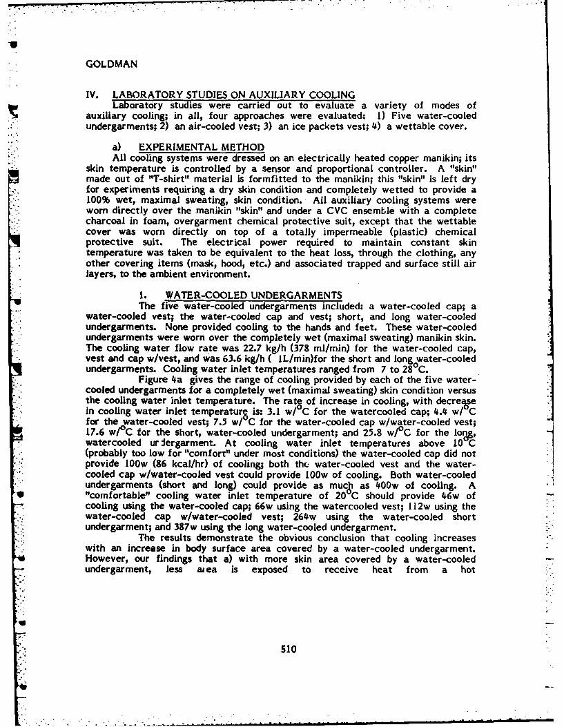
GOLDMAN
IV. LABORATORY STUDIES ON AUXILIARY COOLINGLaboratory studies were carried out to evaluate a variety of modes of
auxiliary cooling; in all, four approaches were evaluated: 1) Five water-cooledundergarments; 2) an air-cooled vest; 3) an ice packets vest; 4) a wettable cover.
a) EXPERIMENTAL METHODAll cooling systems were dressed on an electrically heated copper manikin; its
skin temperature is controlled by a sensor and proportional controller. A "skin"made out of "T-shirt" material is formfitted to the manikin; this "skin" is left dryfor experiments requiring a dry skin condition and completely wetted to provide a100% wet, maximal sweating, skin condition. All auxiliary cooling systems wereworn directly over the manikin "skin" and under a CVC ensemble with a completecharcoal in foam, overgarment chemical protective suit, except that the wettablecover was worn directly on top of a totally impermeable (plastic) chemicalprotective suit. The electrical power required to maintain constant skintemperature was taken to be equivalent to the heat loss, through the clothing, anyother covering items (mask, hood, etc.),and associated trapped and surface still airlayers, to the ambient environment.
1. WATER-COOLED UNDERGARMENTSThe five water-cooled undergarments included: a water-cooled cap; a
water-cooled vest; the water-cooled cap and vest; short, and long water-cooledundergarments. None provided cooling to the hands and feet. These water-cooledundergarments were worn over the completely wet (maximal sweating) manikin skin.The cooling water flow rate was 22.7 kg/h (378 ml/min) for the water-cooled cap,vest and cap w/vest, and was 63.6 kg/h ( IL/min)for the short and long water-cooledundergarments. Cooling water inlet temperatures ranged from 7 to 28 C.
Figure 4a gives the range of cooling provided by each of the five water-cooled undergarments for a completely wet (maximal sweating) skin condition versusthe cooling water inlet temperature. The rat 8 of increase in cooling, with decreasein cooling water inlet temperaturs is: 3.1 w/ C for the watercooled cap; 4.4 w/ Cfor the water-cooled vest; 7.5 w/ C for the water-cooled cap w/water-cooled vest;17.6 w/ 0 C for the short, water-cooled undergarment; and 25.8 w/°C for the long,
* watercooled ur iergarment. At cooling water inlet temperatures above 10 Ct(probably too low for "comfort" under most conditions) the water-cooled cap did notprovide 100w (86 kcal/hr) of cooling; both th* water-cooled vest and the water-cooled cap w/water-cooled vest could provide 100w of cooling. Both water-cooledundergarments (short and long) could provide as muc as 400w of cooling. A
"* "comfortable" cooling water inlet temperature of 20 C should provide 46w of.-cooling using the water-cooled cap; 66w using the watercooled vest; 112w using thewater-cooled cap w/water-cooled vest; 264w using the water-cooled shortundergarment; and 387w using the long water-cooled undergarment.
The results demonstrate the obvious conclusion that cooling increaseswith an increase in body surface area covered by a water-cooled undergarment.However, our findings that a) with more skin area covered by a water-cooled
* undergarment, less ai ea is exposed to receive heat from a hot
510
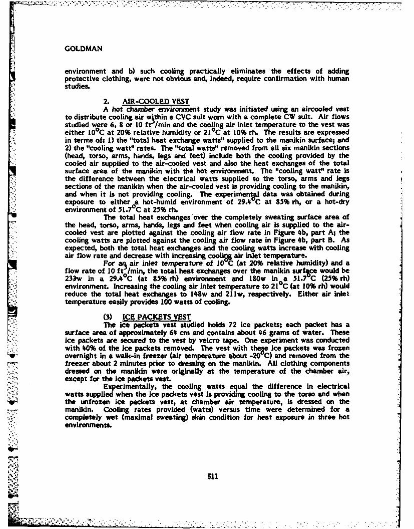
GOLDMAN
environment and b) such cooling practically eliminates the effects of addingprotective clothing, were not obvious and, indeed, require confirmation with humanstudies.
2. AIR-COOLED VESTA hot chamber environment study was initiated using an aircooled vest
to distribute cooling air within a CVC suit worn with a complete CW suit. Air flowsstudied were 6, 8 or 10 ft /min and the cooling air inlet temperature to the vest waseither 10°C at 20% relative humidity or 21 0C at 10% rh. The results are expressedin terms of: 1) the "total heat exchange watts" supplied to the manikin surface; and2) the "cooling watt" rates. The "total watts" removed from all six manikin sections(head, torso, arms, hands, legs and feet) include both the cooling provided by thecooled air supplied to the air-cooled vest and also the heat exchanges of the totalsurface area of the manikin with the hot environment. The "cooling watt" rate isthe difference between the electrical watts supplied to the torso, arms and legssections of the manikin when the air-cooled vest is providing cooling to the manikin,and when it is not providing cooling. The experimentai data was obtained duringexposure to either a hot-humid environment of 29.4 C at 85% rh, or a hot-dryenvironment of 51.7°C at 25% rh.
The total heat exchanges over the completely sweating surface area ofthe head, torso, arms, hands, legs and feet when cooling air is supplied to the air-cooled vest are plotted against the cooling air flow rate in Figure 4b, part A; thecooling watts are plotted against the cooling air flow rate in Figure 4b, part B. Asexpected, both the total heat exchanges and the cooling watts increase with coolingair flow rate and decrease with increasing cooli 8g air inlet temperature.
For a air inlet temperature of 10 C (at 20% relative humidity) and aflow rate of 10 ft min, the total heat exchanges over the manikin surfae would be233w in a 29.4 C (at 85% rh) environment and 180w inoa 51.7 C (25% rh)environment. Increasing the cooling air inlet temperature to 21 C (at 10% rh) wouJ4reduce the total heat exchanges to 148w and 211w, respectively. Either air inlettemperature easily provides 100 watts of cooling.
(3) ICE PACKETS VESTThe ice packets vest studied holds 72 ice packets; each packet has a
surface area of approximately 64 cm and contains about 46 grams of water. Theseice packets are secured to the vest by velcro tape. One experiment was conductedwith 40% of the ice packets removed. The vest with t her ice packets was frozenovernight in a walk-in freezer (air temperature about -20 C) and removed from thefreezer about 2 minutes prior to dressing on the manikin. All clothing components
- dressed on the manikin were originally at the temperature of the chamber air,except for the ice packets vest.
Experimentally, the cooling watts equal the difference In electricalwatts supplied when the ice packets vest is providing cooling to the torso and whenthe unfrozen ice packets vest, at chamber air temperature, is dressed on themanikin. Cooling rates provided (watts) versus time were determined for acompletely wet (maximal sweating) skin condition for heat exposure In three hotenvironments.
io.-1
'*% ":S
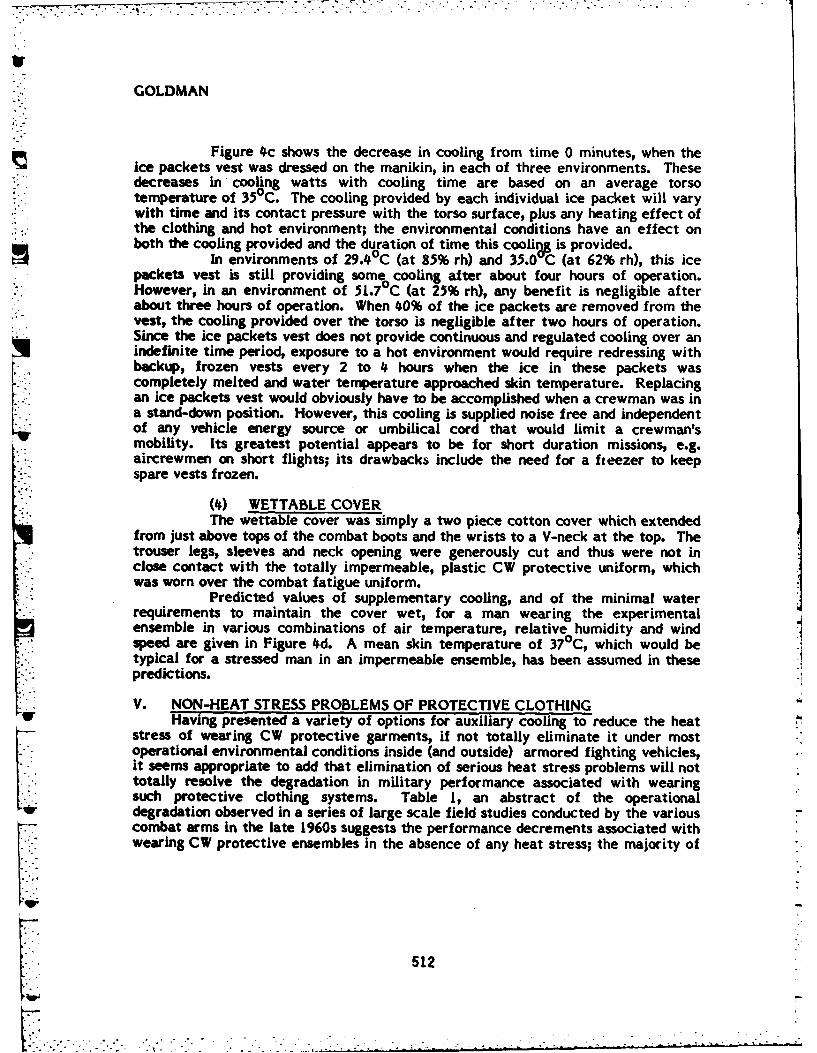
GOLDMAN
Figure 4c shows the decrease in cooling from time 0 minutes, when theice packets vest was dressed on the manikin, in each of three environments. Thesedecreases in cooling watts with cooling time are based on an average torsotemperature of 350 C. The cooling provided by each individual ice packet will varywith time and its contact pressure with the torso surface, plus any heating effect ofthe clothing and hot environment; the environmental conditions have an effect onboth the cooling provided and the duration of time this coolinA is provided.
In environments of 29.4°C (at 85% rh) and 35.0 C (at 62% rh), this icepackets vest is still providing some cooling after about four hours of operation.However, in an environment of 51.7 C (at 25% rh), any benefit is negligible afterabout three hours of operation. When 40% of the ice packets are removed from thevest, the cooling provided over the torso is negligible after two hours of operation.Since the ice packets vest does not provide continuous and regulated cooling over anindefinite time period, exposure to a hot environment would require redressing withbackup, frozen vests every 2 to 4 hours when the ice in these packets wascompletely melted and water temperature approached skin temperature. Replacingan ice packets vest would obviously have to be accomplished when a crewman was ina stand-down position. However, this cooling is supplied noise free and independentof any vehicle energy source or umbilical cord that would limit a crewman'smobility. Its greatest potential appears to be for short duration missions, e.g.aircrewmen on short flights; its drawbacks include the need for a freezer to keepspare vests frozen.
(4) WETTABLE COVERThe wettable cover was simply a two piece cotton cover which extended
from just above tops of the combat boots and the wrists to a V-neck at the top. Thetrouser legs, sleeves and neck opening were generously cut and thus were not inclose contact with the totally impermeable, plastic CW protective uniform, whichwas worn over the combat fatigue uniform.
Predicted values of supplementary cooling, and of the minimal waterrequirements to maintain the cover wet, for a man wearing the experimentalensemble in various combinations of air temperature, relative humidity and windspeed are given in Figure 4d. A mean skin temperature of 37°C, which would betypical for a stressed man in an impermeable ensemble, has been assumed in thesepredictions.
V. NON-HEAT STRESS PROBLEMS OF PROTECTIVE CLOTHINGHaving presented a variety of options for auxiliary cooling to reduce the heat
stress of wearing CW protective garments, if not totally eliminate it under mostoperational environmental conditions inside (and outside) armored fighting vehicles,it seems appropriate to add that elimination of serious heat stress problems will nottotally resolve the degradation in military performance associated with wearingsuch protective clothing systems. Table 1, an abstract of the operational
•*r degradation observed in a series of large scale field studies conducted by the variouscombat arms in the late 1960s suggests the performance decrements associated withwearing CW protective ensembles in the absence of any heat stress; the majority of
512
GOLDMAN
these resIt from mechanical barriers to sensory inputs to the wearer and to barriersfor communication between individuals. By redesigning the maneuver scenariosprepared initially by the various combat arms, heat stress was essentiallyeliminated, and it became feasible to assess other forms of performancedecrements. The table compares the performance of troops wearing 1) normalcombat clothing and equipment (MOP I), 2) CW protective ensembles "open", i.e.without hood, gloves and with all apertures open, but with gas mask (MOP I) or 3)fully encapsulated (MOP III) with mask, hood and gloves, and all uniform openingssealed, for four critical elements of combat: 1) fire power, 2) communications, 3)mobility and 4) support. There is a great deal of variability in the results of anysuch "large scale maneuver" field studies of operational performance, and some ofthe expected "overcompensation" can be noted; i.e. performance is actuallyimproved slightly by imposing impediments that the troops are aware of and canmake adjustment for. However, overall it is clear that elimination of heat stress,while it will allow mission performance to continue, will not totally eliminate theconstraints imposed by CW protective clothing systems.
REFERENCES
Goldman, R.F. Tolerance time for work in the heat when wearing CBR protectiveclothing. Mil. Med. 128:776-786, 1963.
Joy, R.J.T. and R.F. Goldman. A method of relating physiology and militaryperformance: A study of some effects of vapor barrier clothing in hot climate. Mil.Med. 133:458-470, 1968.
Martin, H de V. and R.F. Goldman. Comparison of physical, physiological methodsof evaluating the thermal stress associated with wearing protective clothing.Erzonomics 15:337-342, 1972.
Breckenridge, 3.R. and R.F. Goldman. Effect of clothing on bodily resistanceagainst meterological stimuli. Progress in Biometeorolotty. Vol. 1, Part I1, Section19, 194-208, Chap. 7, 1977.
Shapiro, Y., K.B. Pandolf, M.N. Sawka, M.M. Toner, F.R. Winsmann and R.F.Goldman. Auxiliary Cooling: Comparison of air-cooled versus water-cooled vest inhot-dry and hot-wet environments. Aviat. Space and Environ. Med. In press,Apr/May 1982.
The views, opinions, and/or findings contained in this report are those of theauthor(s) and should not be construed as an official department of the Armyposition, policy, or decision, unless so designated by other official documentation.
Human subjects paticipated in these studies after giving their free andinformed voluntary consent. Investigators adhered to AR 70-25 and USAMRDCRegulation 70-25 on Use of Volunteers in Research.
513
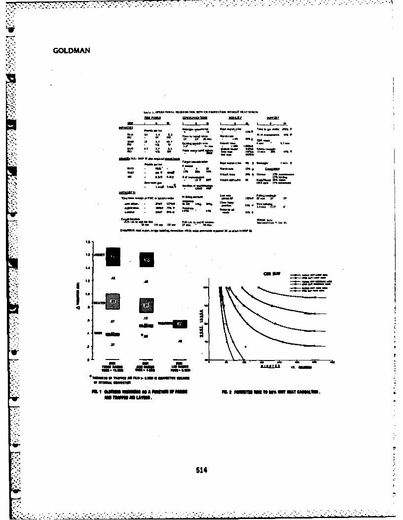
GOLDMAN
Q.b. .IIT9AI. ac"10,100 UYK COPfaewit~ UTKOUT ICA& 11M99
murng cM M~cal &ff1 y3
UU IA I -- .- I. 1. m. m0 4 I I
fin T .p I - 2v .99.1 .a60 as9949~&m Co-3~6. .
It It .0 A. '.2
W" ml on* 13% amU5 "h i 16 tQ
wn Vote )99II SW m VA :
W9.l 199 .11 C 991191 F.4 w. SIaea bui-35IS V tti. test.~499 In
NO.WP116016M-V6I0 WW MinISl 7354 314i. 0 5U1.40 K~ 9I
ts99 JAM a
IA99999~a.141 3959
-~A ...lmi
V. dm 3#@ai.e 7~S1
umm MAWii .. -Z-&u
w Mum
-2
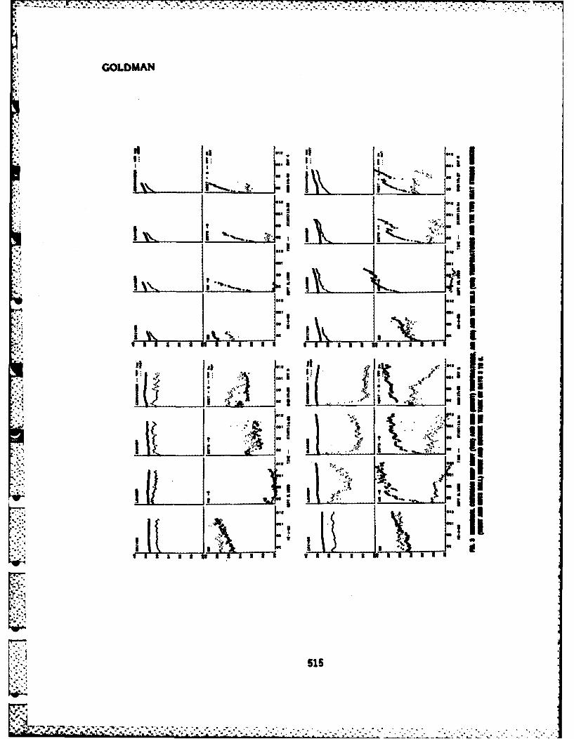
A
GOLDMAN
G.s
.4.b
OS'
mi %... in . ..
itI '. .-' , |
*
m ,., ,l. I,.
I p I I
' I ,a ,. *' ii '
P:~
•
N!~
I I
iI .ll Ii.i * ... II
II i II II I*'l i I
6 515
....................
.- .......
-%-~-~--.---..-.-.-... ~ . .... ...

kmm
5 I s I
-4
a* =VN :M N
GOODRICK-w
DEVELOPMENT OF METHODS FOR ASSESSMENTOF GLIDING PARACHUTE APPLICATIONS
TUGIA F.* GOODRICK.US AWM NATICK R&D) LABORATORIES
NATICK, MASSACHUSETTS 01760
In order to assess the possible utility of gliding parachutes, it wasnecessary to develop a set of methods for predicting behavior of glidingparachutes. Gliding parachutes presented some unique problems not coveredby the technology base existing in 1968. At that time a few brave Jumperswere experimenting with squares. The Army was encountering difficulty Inobtaining consistent performance from a small gliding system for cargo. Onsome days it worked; on others it did not. Engineers with parachute exper-ience viewed the problem mainly as inconsistent deployment. Engineers withaircraft experience thought the problem was poor navigation and lack ofpower. Neither field of engineering was wholly appropriate.
Based on the observations that canopy opening was not too differentfrom conventional parachutes in most critical respects and that canopiestended to glide with reasonable steadiness, we chose to concentrate firston the problem of guidance. As a first step, we worked out a graphical(manual) method of plotting trajectory points for a gliding canopy driftingwith the wind while homing on a target. A visiting student helped with themanual labor. Soon we transferred the technique to a programed calculatorthough graphs still had to be drawn by hand. The technique was crude, butit effectively demonstrated some key features of radial homing as appliedto low-speed gliding parachutes .(l) This was our first use of "computer"simulation. Later we moved to a fancier programable calculator with anX-Y plotter and studied more exotic guidance schmes.(2)(3)
However, as we investigated guidance schemes it became obvious that weneeded more knowledge of the flight dynamics of gliding parachutes. Pub-lished test data was inadequate. A test program appeared to be too expen-sive and time-consuming. Also, we were not sure what parameters should bemeasured in testing - nor how to measure them. Thus, we began the develop-
-" neat of analytical and computational techniques for study of all aspects ofgliding canopies. This development effort has included models for study oflongitudinal stability and for study of unrestricted flight in siz-degres-
517
................... 1dilidlI - ~m~ i '- h :.... nn" "rF - ... .
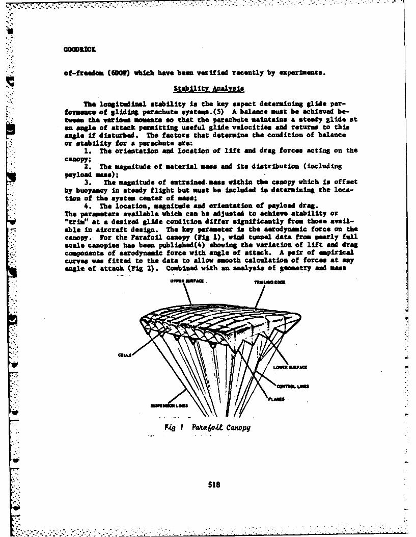
of-fredom (EDO!) which have been verifiled recently by experiments.
Stability Analysis
The longitudinal stability Is the key aspect determining Slide per-formance of gliding parachute systums. (5) A balance mot be achieved be-twee. the various moments so that the parachute maintainsa steady glide atan angle of attack permitting useful glide velocities and returns to thisangle If disturbed. The factors that determine the condition of balanceor stability for a parachute are:
1. The orientation and location of lift and drag forces acting on thecanopy;
2. The magnitude of material asse and Its distribution (includingpayload mass);
3. The magnitude of entrained. mass within the canopy which is offsetby buoyancy In steady flight but must be Included in determining the loca-tion of the systas center of mass;
4. The location, magnitude and orientation of payload drag.The parameters available which can be adjusted to achieve stability or"trim" at a desired glide condition differ significantly from those avail-able In aircraft design. The key paramter Is the aerodynamic force. on thecanopy. For the Farafoil canopy (FIX 1), wind tunnel data from nearly fullscale canopies has been published(4) showing the variation of lift and dregcomponents of aerodynamic force with angle of attack. A pair of ampiricaLcurves was fitted to the data to allow smooth calculation of forces at anyangle of attack (Fig 2). Combined with an analysis of somet%7 and mass
UPPER VAMZm~ n
F4 1 PakdJoiI Canopy
518
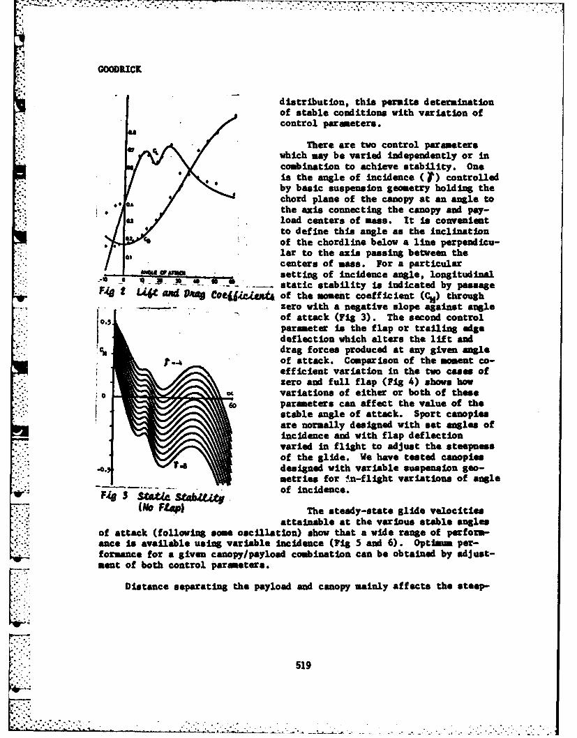
GOODRICK
distribution, this permits determinationof stable conditions with variation ofcontrol parameters.
There are two control parametersCwhich may be varied independently or in
combination to achieve stability. Oneis the angle of Incidence (l)controlledby basic suspension geometry holding thechord plane of the canopy at an angle to
- . the axis connecting the canopy and pay-63 load centers of mas. It is convenient
to define this angle as the inclinationof the chordline below a line perpendicu-
lar to the axis passing between thecenters of mass. For a particularsetting of incidence angle, longitudinal
" ;. - - static stability is indicated by passageUg I AA4t a W P&V C OU&Lejti of the moment coefficient (C) through
zero with a negative slope against angle
0.5 of attack (Fig 3). The second controlparameter is the flap or trailing edgedeflection which alters the lift anddrag forces produced at any given angle
't-.4 'of attack. Comparison of the moment co-efficient variation in the two cases ofzero and full flap (Fig 4) shows how
"0 variations of either or both of these-6- parameters can affect the value of the
stable angle of attack. Sport canopiesare normally designed with set angles ofincidence and with flap deflectionvaried n flight to adjust the steepnessof the Slide. We have tested canopiesdesigned with variable suspension Seo-metries for in-flight variations of angleof incidence.
0.--6N Fp The steady-state glide velocitiesattainable at the various stable angles
of attack (following some oscillation) show that a wide range of perform-ance is available using variable incidence (Fig 5 and 6). Optimum per-formance for a given canopy/payload combination can be obtained by adjust-ment of both control parameters.[I" -Distance separating the payload and canopy mainly affects the steep-
Li 519
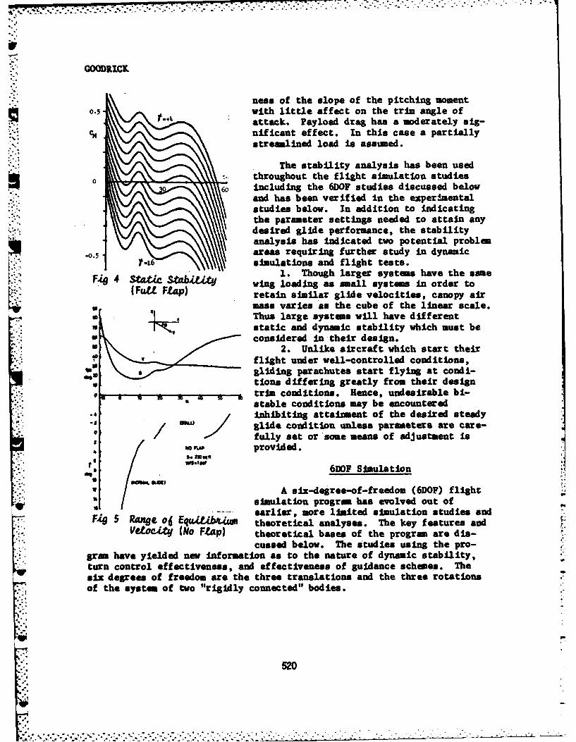
GOODRICX
ness of the slope of the pitching moment0.5 with little affect on the trim angle of
attack. Payload drag has a moderately sig-CH nificant effect. In this case a partially
streamlined load is assumed.
The stability analysis has been used
. throughout the flight simulation studies6 including the 6DOF studies discussed below
and has been verified in the experimentalstudies below. In addition to indicatingthe parameter settings needed to attain anydesired glide performance, the stabilityanalysis has indicated two potential problem
-0.5 areas requiring further study in dynamic--16 simulations and flight tests.
1. Though larger systems have the saneFAQ 4 SW StabAV4 wing loading as small systems in order to
(FaU FLap) retain similar glide velocities, canopy air
mass varies as the cube of the linear scale.Thus large systems will have different
* static and dynamic stability which must beconsidered in their design.
2. Unlike aircraft which start theirflight under well-controlled conditions,gliding parachutes start flying at condi-tions differing greatly from their design
"e trim conditions. Hence, undesirable bi-., stable conditions may be encountered
.-, inhibiting attainment of the desired steady. / glide condition unless paraseters are care-
fully set or some means of adjustment Is"D rip provided.
' lS. =94e I.
• -,... 6DOF Simulation
' A six-degree-of-freedom (6DOF) flightsimulation program has evolved out ofearlier, more limited simulation studies and
F- 5 Rnge oJ Equt ~b#.m theoretical analyses. The key features and
VttOci4 (No FLapi theoretical bases of the program are dis-cussed below. The studies using the pro-
gram have yielded new Information as to the nature of dynamic stability,turn control effectiveness, and effectiveness of guidance schemes. Thesix degrees of freedom are the three translations and the three rotations
of the system of two "rigidly connected" bodies.
520
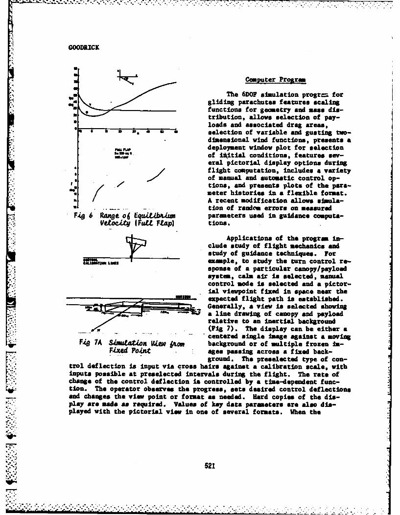
GOODRICK
Computer Program
gli1The 6DOF simulation progr- forgiding parachutes features scalingfunctions for geometry and mass dis-tribution, allows selection of pay-
___loads and associated drag areas,0 a a , *Z * a selection of variable and gusting two-
* dimensional wind functions, presents ann deployment window plot for selections.t of inktial conditions, features sew-
eral pictorial display options duringflight computation, includes a varietyof manual and automatic control op-tions, and presents plots of the para-meter histories in a flexible format.A recent modification allows simula-tion of random errors on measured
F9 6 Range o6 EquitWm parameters used in guidance computa-Vetocity M~u Ftap) tions.
Applications of the progre in-clude study of flight mechanics and
__________study of guidance techniques. Forl-- s example, to study the turn control re-
sponse of a particular canopy/payloadsystem, calm air is selected, manualcontrol node Is selected and a pictor-ial viewpoint fixed In space near theexpected flight path is established.Generally, a view is selected showing
'; a line drawing of canopy and payloadrelative to an inertial background(Fig 7). The display can be either a
. centered single image against a movingF49 7A Skwtation V.L1w itom background or of multiple frozen im-
Fixed Poi" ages passing across a fixed back-ground. The preselected type of con-
trol deflection is input via cross hairs against a calibration scale, withInputs possible at preselected intervals during the flight. The rate ofchange of the control deflection is controlled by a time-dependent func-tion. The operator observes the progress, sets desired control deflections
__ and changes the view point or format as needed. Hard copies of the dis-play are made as required. Values of key data parameters are also dis-played with the pictorial view in one of several formats. When the
521W %
.o . . . .
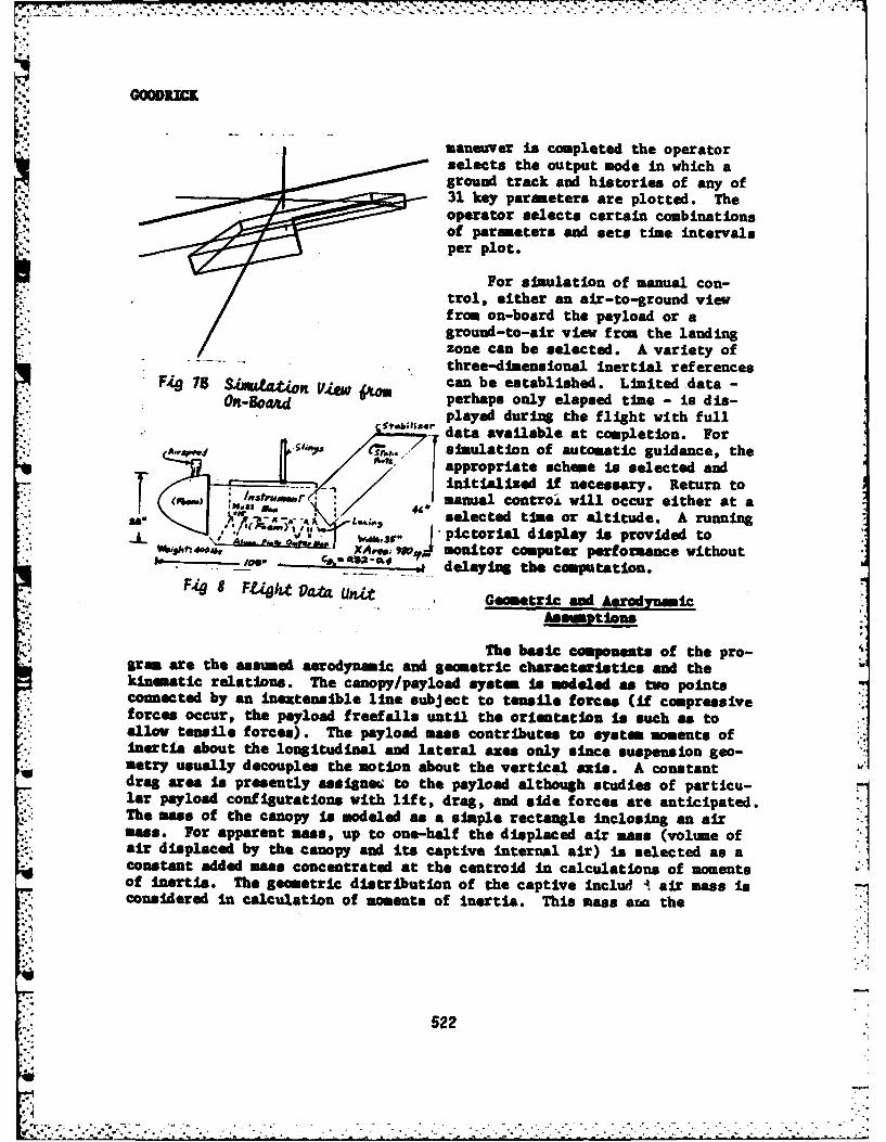
;-, GOODREKi
maneuver is completed the operatorselects the output mode in which aground track and histories of any of31 key parameters are plotted. Theoperator selects certain combinationsof parameters and sets time intervalsper plot.
For simulation of manual con-trol, either an air-to-ground viewfrom on-board the payload or aground-to-air view from the landingzone can be selected. A variety ofthree-dimensional inertial references
U9 75 o VimJJ can be established. Limited data -On-Boakd perhaps only elapsed time - is dis-
played during the flight with full' T" data available at completion. For
Asp, simulation of automatic guidance, theappropriate scheme is selected and
It, 49 manual control wil occur either at a
240 selected time or altitude. A running_ pictorial display Is provided to
W~ugD&l Pu0fti X W monitor computer performance withoutln_- .. : delaying the computation.
Fl9 S F&.. Data u,..t Gemetric and AerodynmicAsemtions:*
The basic components of the pro-arem are the assumed aerodynamic and geometric characteristics and thekinematic relations. The canopy/payload system is modeled as two pointsconnected by an nextensible line subject to tensile forces (if compressiveforces occur, the payload freefalls until the orientation is such as toallow tensile forces). The payload mass contributes to systm moments ofInertia about the longitudinal and lateral axes only since suspension geo-metry usually decouples the otion about the vertical axis. A constantdrag area is presently asaignem; to the payload although studies of particu-1ar payload configurations with lift, drag, and side forces are anticipated.The mass of the canopy is modeled as a simple rectangle inclosing an airms. For apparent mass, up to one-half the displaced air mass (volume ofair displaced by the canopy and its captive internal air) is selected as aconstant added ms concentrated at the centrod in calculations of momentsof Inertia. The geometric distribution of the captive includ i air mass Isconsidered in calculation of moments of inertia. This mass ara the
522
. .,. . . . . . .*
. . . . . . . . . . .
.4~~ - -.. -. - - - - - -
GOODRICK
apparent mass change with altitude according to ambient density.
- .:, Certain unique assumptions have been made in the treatment of aero-dynamic forces and moments. Empirical functions were developed for thebasic wing lift and drag coefficients of Parafoil canopies measured in thewind tunnel. A side force coefficient varying with the sine of the sideslip angle was also extracted from the wind tunnel data. Early attempts toincorporate these coefficients and other moment coefficients and stabilityderivatives measured in the wind tunnel under static conditions failed togive realistic results. Extremely low turn rates were noted under sometypical quasi-steady conditions even though the data supposedly reflectedthe conditions of control deflection. Realistic performance - as comparedwith motion pictures of jumpers and limited available test data - wasfinally achieved by treating the canopy as geometrically distributed seg-ments including spanwise curvature with local lift and drag computed foreach segment based on local velocity and angle of attack. Local lift co-efficients vary from the total wing lift coefficients in a manner approxi-mating an elliptical distribution. The empirical functions for total vinlift and drag coefficients include effects of trailing edge deflections.To study turn and pitch (or "braking") control with trailing edge deflec-tion, the deflection is applied via the empirical functions at selectedsegments. It is important to note that, due to the spanwise curvature, re-sultant aerodynamic forces on deflected segments may be significantly in-clined to the vertical-longitudinal plane.
A study using a separate computer program was made of the quasi-staticstability effects of typical velocity and angle of attack distributionsresulting from the segmentation of the wing. It was found that for typicalwing geometries associated with payloads from 200 to 2000 pounds, theeffects of velocity distribution were highly stabilizing.(6)
Expermental Verification of Simulation
To verify the simulation program a flight test was performed using aParafoil canopy of 200 sq ft (18.6 sq m) and a payload of 380 lbs (165 Kg)
. specially designed to measure those key parameters needed for verification.The emphasis of the test program was on dynamic flight conditions associatedwith turning maneuvers. The payload included remote radio control hard-
--. ware manually activated from the ground.
Flight Data Unit
* The flight data unit (FDU) serving as the payload consists of an inner-. box cushioned within an outer shell to which a specially shaped foam nose
cone and stabilizing tail fins are attached (Fig 8). The geometry of thefins and nose cone was determined during wind tunnel tests to achieve good
523
... .. . .. . .. ..,. . . . . . . ..... . . .
GOODRICK
static and dynamic stability. For accurate airspeed and gyro data the pay-load must track accurately with the canopy. The payload must also trackwell when carried by sling below a helicopter.
A J-Tec vortex-sensing airspeed indicator is mounted on the upper partof the nose cone. Wind tunnel tests were made for calibration at variousangles of attack. Twin static ports in the surface of the vertical finsprovide static pressure for the Rosemount 1241 altimeter with rate output.This mounting arrangement is not affected by moderate slideslip. The brandnames of these units are mentioned because they appear to be the only unitsavailable that are adequate for this application. This was determined inseveral independent surveys. The J-Tec airspeed indicator acousticallysenses the rate of vortex shedding from a special cross-piece in thechanel of the Indicator. It is highly accurate and responsive in the testrange of 10 to 18 a/s. Pressure transducers would be inaccurate in thisrange. The Rosemount altimeter is designed for test applications with goodaccuracy both in altitude and electronically-derived rate measurement.Airspeed and descent rate are the two main parameters of gliding flight.Also, the horizontal component of airspeed can be calculated from the vec-tor difference between total airspeed and descent rate only if each para-meter Is measured accurately.
The FDU alsQ contains three rate gyros on the yaw, pitch end rollaxes. An integrating circuit is attached to the yaw rate gyro to provideapproximate heading data. The gyro data is useful in indicating thenature of turn response which can vary widely depending upon the mechanicsof turn control.
Control deflection is measured from the servo potentiometers.Originally, current draw of the servo motors was measured as an indicationof control force. This has been found unreliable as an indication of forcebecause of electrical transients. Modifications are being made to measureforces from transducers linked to the lines.
A 14-channel PM tape recorder is used to record all signals. A play-back unit re-transforms the IM signal to voltage analog to drive a strip-chart recorder for final copy. The tape recorder Is satisfactory forrecording data during a flu4 it including extreme oscillations. However,it is not satisfactory for recording data under high-shock conditions suchas during deployment and landing. Apparently, the tape is jiggled as itpasses the head when the unit is jolted.
The FDU Is controlled by a model aircraft radio-control system. Theradio-controlled servos drive potentiometers which control the large motorsdrawing In control lines. Currently, two channels are used for turn andglide ratio control. Three motors and lines are used for the left turn,
r
524
• . .
GOODRICK
right turn and glide ratio. The Parafoil is rigged for deflection of thethird (or "C") flare on the second set in from each tip or turn. This pro-duces primarily a roll tilt of the wing with a slight incidence shift. Thetrailing edge Is separately deflected for glide control.
Weight of the payload was 355 pounds during initial testing. Latermodifications added 40 pounds. This weight is carried well by the 200-square-foot Parafoll with unreefed deployment at low speeds (10-30 knots).Landing speed is somewhat high with this loading.
Except for the airspeed indicator, all equipment is housed within theinner box of the FM (35 X 22 X 14 inches). The inner box Is tied to theouter shell at the bottom and surrounded by several Inches of polyurethanefoam. The outer shell is 108 inches overall, including nose and tail witha cross-section of 35 X 28 inches. Drag area (CDS) measured approximatelyn the wind tunnel is 2.15 - 2.69 square feet (0.2 - 0.25 sq i).
Setting System Parameters
Those aspects of the simulation model needing verification included:(1) the lift and drag functions, (2) the model resulting trim conditionpredicted by the longitudinal stability model, (3) the assumption that-linearized moment coefficient and deviations could be replaced by local
force computations at spanwise locations, and (4) the computational ;ech-niques employed. Thus, in matching flight data none of these factors werealtered. input parameters altered for the match, as listed below, werethose parameters not physically measurable. Apparent msas tometimescalled "'virtual" mass) Is a flow !4eld phenomenon - not a physical mass.System length depends on in-flight mass distribution and distorted suspen-sion and canopy geometry. While these parameters could be 'Uallparked",they could not be physically measured. Ideally, to examine flight dynamicsit Is desirable to start from a steady condition. For gliding parachutesthis is impossible. After over twenty flights, steady conditions havenever been observed. Repeatedly, a maneuver mst be entered before theefforts of a previous maneuver have dissipated even though flight appearssteady from the ground. Wind turbulence adds additional disruption. Thetwo flights matched below are the best Illustrations for verification ofthe simulation.
To obtain a reasonable match, the followifg system parameters were.varied in the simulation:
1. Apparent mass coefficient (one corresponds to half the volumetricdisplacement) was Initially assaead to be 1.0. Values of 0, 0.8, 1.0, 1.5,2.0, 3.0 were tried. Finl value Is 1.01
2. Payload drM area (C S) was Initially estimated at 0.4 sq '.
Values of 0.2, 0.25, 0.3, 0.33, 0.4 ware tried. Value selected is .2.
525
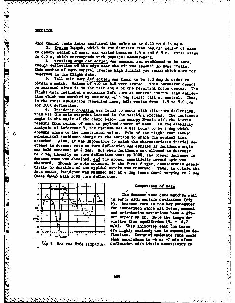
* .- - . ,.
GOODRICK
Wind tunnel tests later confirmed the value to be 0.20 to 0.25 sq m.3. System length, which is the distance from payload center of mass
to canopy center of mass, was varied between 5.5 m and 6.5 m. Final valueis 6.5 a, which corresponds with physical measurement.
4. Traling edge deflection was assumed and confirmed to be zero,though deflection of the edge near the tip was assumed in some trails.This method of turn control creates high initial yaw rates which vere notobserved n the flight data.
5. Roll-tilt turn deflection was found to be 5.0 deg in order toobtain a match. Values of 4.0 to 6 40 were tested. This parameter cannotbe measured since it Is the tilt angle of the resultant force vector. Theflight data indicated a moderate left turn at neutral control line deflec-tion which was matched by assuming -1.5 deg (left) tilt at neutral. Thus,in the final simulation presented here, tilt varies from -1.5 to 5.0 degfor 100% deflection.
6. Incidence couplinst was found to occur with tilt-turn deflection.This was the main surprise learned in the matching process . The incidenceangle Is the angle of the chord below the canopy X-axis with the Z-axispassing from center of mass to payload center of mass. In the stabilityanalysis of Reference 3, the optImm value was found to be 4 deg whichappears close to the constructed value. Film of the flight test showedsubstantial ncidence change of the section to which the control lineattached. Also, it was Impossible to match the characteristic initial de-crease in descent rate as turn deflection was applied if incidence anglewas held constant at 4 deg. But when incidence was allowed to decreaseto 2 deg linearly as turn deflection went to 100Z, the proper decrease in
. descent rate was obtained, and the proper sensitivity toward spin wasobserved. Though no spin occurred in the first flight, considerable sensi-tivity to duration of the applied stroke was observed. Thus, to obtain thedata match, Incidence was assumed set at 4 deg (nose down) varying to 2 deg(nose down) with 10OZ turn deflection.
-. Comparison of Data
- - - /The descent rate data matches well-In parts with certain deviation@ (Fig
4 -IN 9). Descent rate s the key parameterfor couarison since all force, moment
.. and orientation variations have a dir-- - .L..•act effect on it. Note the lare de-
:--- - viation from equilibritm (V. - -t.7 I'a/0/s). This indiates that he turms
"" g .u m are highly unsteady Ame to excessive do-flection. Turns, of morate rate umldshmw excursions to -6 or -7 w/o after7F4 9 Pueent Ra.te (Exp/Sim) deflection with little smeitivity to
m.
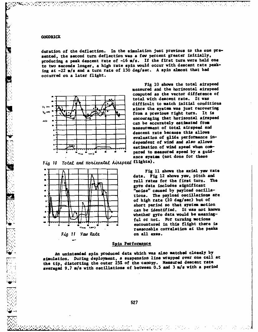
GOODRICK
duration of the deflection. In the simulation just previous to the one pre-sented, the second turn deflection was a few percent greater initially,
producing a peak descent rate of -16 v/s. If the first turn were held one
to two seconds longer, a high rate spin would occur with descent rate peak-
ing at -22 u/s and a turn rate of 150 deg/sec. A spin almost that bad
occurred on a later flight.
Fig 10 shows the total airspeedmeasured and the horizontal airspeed
- computed as the vector difference of
F t I total with descent rate. It was* - difficult to match initial conditions
- since the system was just recovering. from a previous right turn. It is
- - encouraging that horizontal airspeed- - - - can be accurately estimated from
measurement of total airspeed anddescent rate because this allows
evaluation of glide performance in--- - -- - - dependent of wind and also allows
estimation of wind speed when com-* . --. ) - -pared to measured speed by a guld-
ance system (not done for these
FU 10 ToWt ti and HoxizoW A /tpeed flights).
Fig 11 shows the axial yaw rate
data. Fig 12 shows yaw, pitch and-- roll rates for the first turn. The
* -- -gyro data includes signficant-" l -"noise" caused by payload oscilla-
-•- - : tions. The payload oscillations areS -- : • of high rate (10 deg/sec) but of
.-- - short period so that system notionScan be identified. It was not known
- - whether gyro data would be meaning-ful or not. For turning notionsencountered in this flight there isreasonable correlation at the peaks
F~g 11 Yaw Rate on all axes.K" Spin Performance
An unintended spin produced data which was also matched closely by
7_7 simulation. During deployment, a suspension line wrapped over one cell at
the tip, distorting the outer 25% of the canopy. Measured descent rate
averaged 9.7 m/s with oscillations of between 0.5 and 3 m/s with a period
. --"" ""-"527
r 7:o
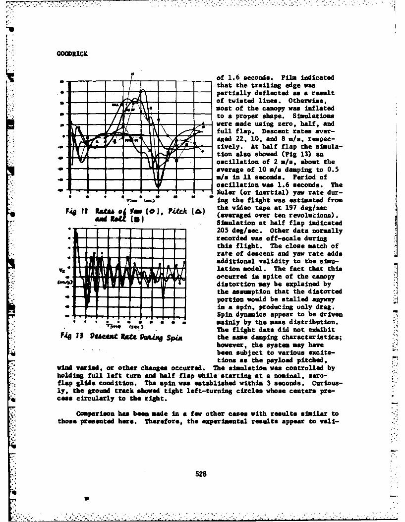
GOODRICK
_ of 1.6 seconds. Film indicatedthat the trailing edge was
* , - partially deflected as a result-- - - of twisted lines. Otherwise,
most of the canopy was inflatedto a proper shape. Simulations
- were made using zero, half, andfull flap. Descent rates aver-
* - aged 22, 10, and 8 ms, respec-tively. At half flap the simula-tion also shoved (Fig 13) an
S V oscillation of 2 m/s, about thea --- verage of 10 m/s damping to 0.5
-i-mi.s I 11 seconds. Period ofoscillation was 1.6 seconds. The
• . . Muler (or inertial) yaw rate dur-V- " e. " gIn the flight was estimated from
F46 I v.a t ) c( the video tape at 197 deg/secF & I( (averaged over ten revolutions).
Simulation at half flap indicated205 dog/sec. Other data normallyrecorded was off-scale during
this flight. The close match ofrate of descent and yaw rate addsadditional validity to the simu-
vi Vlation model. The fact that thisoccurred in spite of the canopydistortion may be explained bythe assumption that the distortedportion would be stalled anywayin a spin, producing only drag.
.6 .; . -** Spin dymnics appear to be drivenmainly by the mass distribution.The flight data did not exhibit
F 13 VU"A . t R&U t in Spix the same damping characteristics;however, the system may havebeen subject to various excita-tions as the payload pitched,
wind varied, or other changes occurred. The simulation was controlled byholdIn full left turn and half flap while starting at a nominal, zero-flap slide condition. The spin was established within 3 seconds. Curious-ly, the ground track showed tight left-turning circles whose centers pre-cess circularly to the right.
Comparison has been made in a few other cases with results similar tothose presented here. Therefore, the experimental results appear to vali-
528
. . . ... .+ , , -.. .- .. .. ... . . . ....... , ...- .-. . .. . . ... . ... .. . . ,- .+.. .•q -+ , • " + ... - -, + . , . . . .
+
' + .-

/7
GOODRCK
date the simulation program as applied to a 200-square foot Parafoil ofaspect ratio of 2.0 with a 350-pound payload. This conclusion is warranted
because:1. Due to the discrete character of control Inputs, response is
driven mainly by aerodynmic and internal properties assumed for the model.2. The combination of multi-axial responses predicted by the model
is in close agreement with experimental results.
bq4 As of this writing, about 10 good data flights have been made. Thesimulation model has matched salient features of most flights. There Issome difficulty when wind changes occur. The data shows a response to adisturbance rather than a control Input without indicating sufficient datafor simulation. This has made it difficult to match flare dynsmics sincethe few flare landings made were accompanied by some wind turbulence. The
- simulation has been used to identify some anomalies such as Incidenceshifts due to line stretch and trim change caused by a pilot chute.
Conclusion
The extent of agreement between simulation and flight data indicaLesthat the primary factors included in the longitudinal stability analysisand in the 6DO simulation are correct. Although the stability analysispredicts only steady-state behavior, it forms the basis required foranalysis of dynamic behavior in the body-fixed XZ plane. The agreementseen n descent rate (Fig 9) would not be possible with an nvalid sta-bility model. Of course, in turning flight during the response immediatelyfollowing the deflection, other factors such as the semed spanwise distri-, bution of lift and drag become predominant. The agreement in yaw rate(Fig 11) best illustrates correctness of this spect of the 6DOF model.The mechanics driving notion during a spin are quite difficult to under-stand; however, the agreement shown in the descent rate (PIS 13) Indicatesthat the mass ratios assumed are accurate and further justifies the assump-tion of spanwise distribution of lift and drag.
In further development activities on gliding parachute systems, the6DOF modeal will serve to guide exploratory work and will be updated formore accurate application to different canopies and to larger systems.
References
1 1. Goodrick, T., 'Widd Effects on Gliding Parachute Systems with Ion-proportional Automatic Homing Control", TR70-28-AD, USA Natik R&D Labors-tories, 1969.
2. Goodrick, T., "Estimation of Wind Effect on Gliding ParachuteCargo Systems Using Computer Simulation", Paper #70-1193, American Insti-tute for Aeronautics and Astronautics (AIM), 1970.
529
3. Goodrick, T., Pearson, A., Murphy, A., "Analysis of Various Auto-matic Homing Techniques for Gliding Airdrop Systems with ComparativePerformance In Adverse Winds", Paper #73-462, American Institute forAeronautics and Astronautics (AIMA), 1973.
4. Ware, George 14. and Hiassell, Jones L. Jr., "Vind Tunnel Investi-gation of Ram-Air-Inflated. All-Flexible Wings of Aspect Ratios 1.0 to 3.0",MASA 7M SX-1923, Langly Research Center, 1969.
5. Goodrick, T., "Theoretical Study of the Longitudinal Stability ofliigbmrPerformance Gliding Airdrop Systems", Paper 175-1394, American Insti-tute for Aeronautics and Astronautics (AIM), 1973.
6. Goodrick, T., "Simulation Studies of the Flight Dynamics of Glid-Ing Parachute Systems", Paper #79-0417, American Institute for Aeronauticsand Astronautics (AIM), 1979.
* 530
GREGORY & PEARSON
ANALYTICAL AND EXPERIMENTAL STUDIES OF THE RESPONSEOF A CYLINDER TO NUCLEAR THERMAL/BLAST LOADS (U)
*FEDERICK H. GREGORY, MR.
RICHARD J. PEARSON, MR.U.S. ARMY BALLISTIC RESEARCH LABORATORY
ABERDEEN PROVING GROUND, MARYLAND 21005
Two phenomena which are emitted from a nuclear weapon, whose targetvulnerability ranges often overlap, are thermal radiation and blast waves.In most situations of interest to the Army, targets are exposed to a highpercentage of the total available thermal pulse prior to blast wave arrival.This sequence of loads is detrimental to the survival of light weightstructures in which significant in-depth heating occurs prior to the blastwave envelopment. There has been evidence that this thermal preheatingcauses enhanced structural damage [1,2].
EXPERIMENT DESCRIPTION
In order to demonstrate these types of synergistic responses and toprovide some quantitative data, three experiments have been conducted onhollow cylinders of aluminum 6061-T6 in the BRL Thermal/Blast Simulator.One experiment was conducted with thermal-only exposure, one with blast-only loading, and one with combined thermal/blast loading. A diagram ofthe Simulator is shown in Figure 1. The target cylinder is clamped at eachend and placed with its axis in a vertical position as shown. The thermalsource is situated downstream from the target to minimize the effects ofthe shock passing through heated air and combustion products. In the con-bined thermal/blast test, the target is rotated through 180* so that theheated side of the target cylinder is exposed to the on-coming shock wave.
The thermal heating of the aluminum cylinder is accomplished by burn-ing of a mixture of aluminum powder and oxygen. Two thin plastic membranesserve to contain the oxygen gas before ignition. The aluminum powder issprayed through nozzles into the oxygen atmosphere and ignited starting
_. with the nozzles farthest from the target. The aluminum oxide particlesresulting from the burn irradiated the near side of the cylinder, raising
4 its temperature by approximately 200*C.
"7-. The shock loading on the cylinder is produced by pressurizing the.. driver section of the shock tube shown in Figure 1 and then explosively
- , 531
. .o'
GREGORY &PEARSON
Ii.
LAo b S
0,,LIi
0 AU
IIJ.
GREGORY & PEARSON
perforating the steel diaphragm at the interface of the driver sectionand the expansion section (Item A in Figure 1). Despite the fact that thethermal source was located downstream from the target, some degradation ofthe leading spike of the shock wave occurred due to the presence of heatedair in the vicinity of the cylinder.
The following measurements were made on the cylinder during the tests:pressure, axial and circumferential strain, temperature, and thermal flux.In addition, .two high speed cameras were used to monitor the sequence ofevents occurring in the simulator. Pre- and post-shot measurements of theradius of the cylinders were made at 384 points on each cylinder. Moredetailed descriptions of the instrumentation are contained in Reference 3.
The cylindrical targets were made from 1.016 um thick sheets ofaluminum 6061-T6, The sheets were formed into cylinders and seam weldedon the side farthest from the loading side. The inside diameter of thecylinders was 30.48 cm (12 inches) and the length between upper and lowerclamps was 80 cm. In order to make the ADINA finite element modeling ofthe experiments easier, the upper and lower ends of the cylinders wereclamped securely in heavy steel end discs. The end discs were connectedby shafts to bearings. The bearings were mounted in two heavy bearingmounts. To minimize the disturbance of the flow past the cylinder, themounts were made with the same outer diameter as the target cylinders.
"UMUICAL MODEL
The numerical modeling of these tests was done with the ADINA finiteelement program [41. The element type used was the 3-D brick element,which has a thermo-elastic formulation. Syetry was assumed about aplane passing through the cylinder axis oriented in the direction of air-heat flow. Another plane of symmetry was assumed passing orthogonal toboth the previous plane and passing through the Z-coordinate L/2, where Lis the active length of the cylinder. With these assumptions, only onequarter of the cylinder was required for the finite element model. Actu-ally, there was approximately a 10 per cent variation in heating along theaxis of the cylinder due to nearby reflecting surfaces. However, thisvariation was Ignored in the numerical simulation.
The quarter cylinder was modeled with 72 brick elements, 8 in theaxial direction, 9 in the circumferential direction, and 1 n the thick-ness direction. The elements had a midside node on each edge and the-nber of integration points in the element was 3 in each direction, fora total of 27 per element. The outside surface of the undeformed mesh isindicated In Figure 2 by the crosses and dotted lines. The crossesrepresent the nodal points on the outside surface and the dotted lines arethe undeformed mesh boundaries.
633
,~... . . . . . .. ,..... ....... : .... •: ...... .. .:.....:.: .. ::.:.:::-:-:-:::-: :-.....,-..,:,
. - -- o• . . -
GREGORY & PEARSON
Figure 2. Mode Shape for the 7th Elgenfrequency (3961 cycles/seconds)
The lower eigenfrequencie8 and mode shapes were evaluated for use ina mode superposition analysis of the elastic response of the cold cylinder.Knowing the periods of the lower eigenfrequencies is also useful indetermining the approximate time required for a peak deflection to occur.The periods determined ranged from 3.66 mas for the lowest mode to 1.47 msfor the eleventh mode. Shown in Figure 2 is mode number seven, which hasthe simpliest geometric shape (egg-shaped cross section).
The finite element calculations for the dynamic response of thecylinder were made using the explicit central difference time marchingscheme. The time step was obtained from the Courant stability condition,
At* At
where At is the distance between the two closest nodes, Ey is Young's
modulus, and p is the material density. For the higher order elementsused here, we found that this time increment was unstable and we used onehalf of the Courant At, which was stable. This time increment was 50 us.
The constitutive properties of the cold aluminum 6061-T6 material4ere measured in an Instron testing machine. Tensile test specimens werecut from the same sheet of material used for fabrication of the cylinders.Properties were measured in the rolling direction and perpendicular to the
534
'- a"
.
GREGORY & PEARSON
rolling direction. The average of these tensile properties was used in theADINA calculations. Properties measured in this way were the Young's modu-lus, bilinear corner yield stress, plastic modulus and Poisson's ratio.
Dynamic temperature dependent constitutive properties were measuredin the DNA Tri-Service Flash Test Facility. In these tests, samples of thematerial were heated in a fraction of a second and strained through theyield point several seconds later. These times were close to the tempera-ture-time sequence experienced in the thermal/blast simulation tests. Theyield points determined in these tests were consistent with other data[5]. However, the plastic tangent moduli appeared to be higher thanexpected. Due to this result and to difficulty in keeping strain gagesbonded at the high temperatures, we chose to await further confirmationprior to using the data. The following temperature dependent stress-straindata have been derived from Reference 5. No temperature dependeft data for
Temperature Density Yield Young's Modulus°C g/cm 3 MPa GPa
28 2.703 301.0 64.73100 2.689 275.4 62.20150 2.678 259.1 60.80200 2.667 240.5 59.29
the plastic tangent modulus and Poisson's ratio were available. The coldproperties measured in the Instron testing machine of 650 MPa and 0.3285,respectively, were used for all temperature ranges.
The ADINA calculations were performed using a bilinear von Miseskinematic hardening material model. This model required the specificationof the materials properties: Young's modulus, Poisson's ratio, initialyield stress, and plastic tangent modulus.
RESULTS
The three types of tests and analyses will be discussed in the sameorder as the experiments were performed. The input head-on pressure forthe blast-only test is shown in Figure 3. The maximum stagnation over-pressure was 60 kPa. Shown in Figure 4 is the short term reflected pres-
.- sure on the cylinder at zero degrees. The peak load is 104 kPa (15 psi).Figure 5 shows the pressure loading on the side of the cylinder (90*).Loading data were recorded at 150 intervals around the cylinder. Sincethe finite element calculations required loading at 200 intervals aroundthe circumference starting at 10, these data were interpolated in both
* .circumferential angle and time to supply the pressure loading for ADINA.
535
. . .
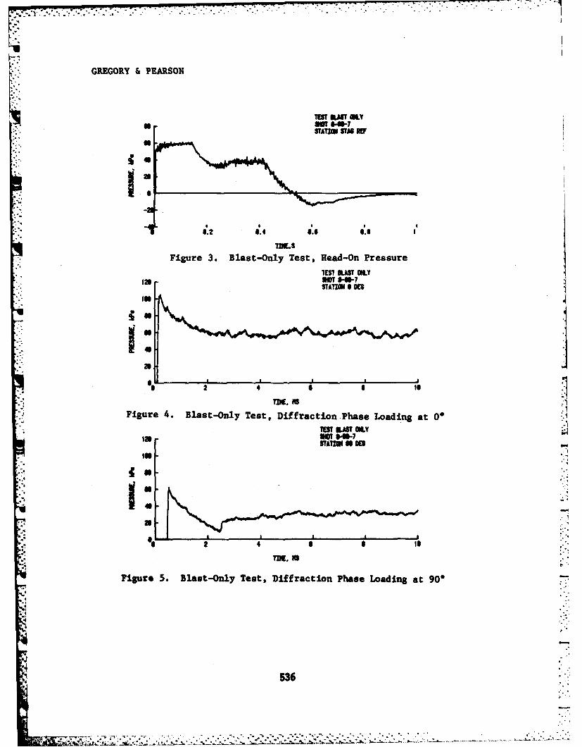
GREGORY &PEARSON
TEST NAIT OLYw * 8641-
STATZI STA IV
.28. 4 .6 a.$6
Figure 3. Blast-Only Test, Head-On Pressure
amR OL
STAIO I
Figure 4. Blast-Only Test, Diffraction Phase Loading at 00
as -4
2 4.
Figure 5. Blast-Only Test, Diffraction Phase Loading at 900
636
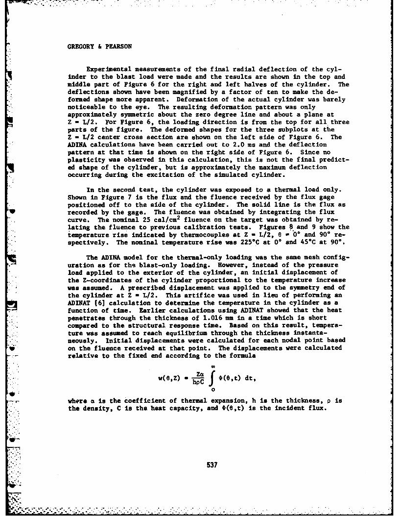
GREGORY & PEARSON
Experimental measurements of the final radial deflection of the cyl-inder to the blast load were made and the results are shown in the top andmiddle part of Figure 6 for the right and left halves of the cylinder. Thedeflections shown have been magnified by a factor of ten to make the de-formed shape more apparent. Deformation of the actual cylinder was barelynoticeable to the eye. The resulting deformation pattern was onlyapproximately symmetric about the zero degree line and about a plane atZ - L/2. For Figure 6, the loading direction is from the top for all threeparts of the figure. The deformed shapes for the three subplots at theZ - L/2 center cross section are shown on the left side of Figure 6. TheADINA calculations have been carried out to 2.0 ms and the deflectionpattern at that time is shown on the right side of Figure 6. Since noplasticity was observed in this calculation, this is not the final predict-ed shape of the cylinder, but is approximately the maximum deflectionoccurring during the excitation of the simulated cylinder.
In the second test, the cylinder was exposed to a thermal load only.Shown in Figure 7 is the flux and the fluence received by the flux gagepositioned off to the side of the cylinder. The solid line is the flux asrecorded by the gage. The fluence was obtained by integrating the flux
-* curve. The nominal 25 cal/cm2 fluence on the target was obtained by re-lating the fluence to previous calibration tests. Figures 8 and 9 show thetemperature rise indicated by thermocouples at Z - L/2, e W"00 and 900 re-spectively. The nominal temperature rise was 225"C at 00 and 45°C at 90.
The ADINA model for the thermal-only loading was the same mesh config-
uration as for the blast-only loading. However, instead of the pressureload applied to the exterior of the cylinder, an initial displacement ofthe Z-coordinates of the cylinder proportional to the temperature increasewas assumed. A prescribed displacement was applied to the symmetry end ofthe cylinder at Z - L/2. This artifice was used in lieu of performing anADINAT (61 calculation to determine the temperature in the cylinder as afunction of time. Earlier calculations using ADINAT showed that the heatpenetrates through the thickness of 1.016 mm in a time which is short
*. compared to the structural response time. Based on this result, tempera-ture was assumed to reach equilibrium through the thickness instanta-neously. Initial displacements were calculated for each nodal point basedon the fluence received at that point. The displacements were calculatedrelative to the fixed end according to the formula
w(e,Z) - hC 0(9,t) dt,
0
where a is the coefficient of thermal expansion, h is the thickness, p isthe density, C is the heat capacity, and 0(6,t) is the incident flux.
537
A A M *%
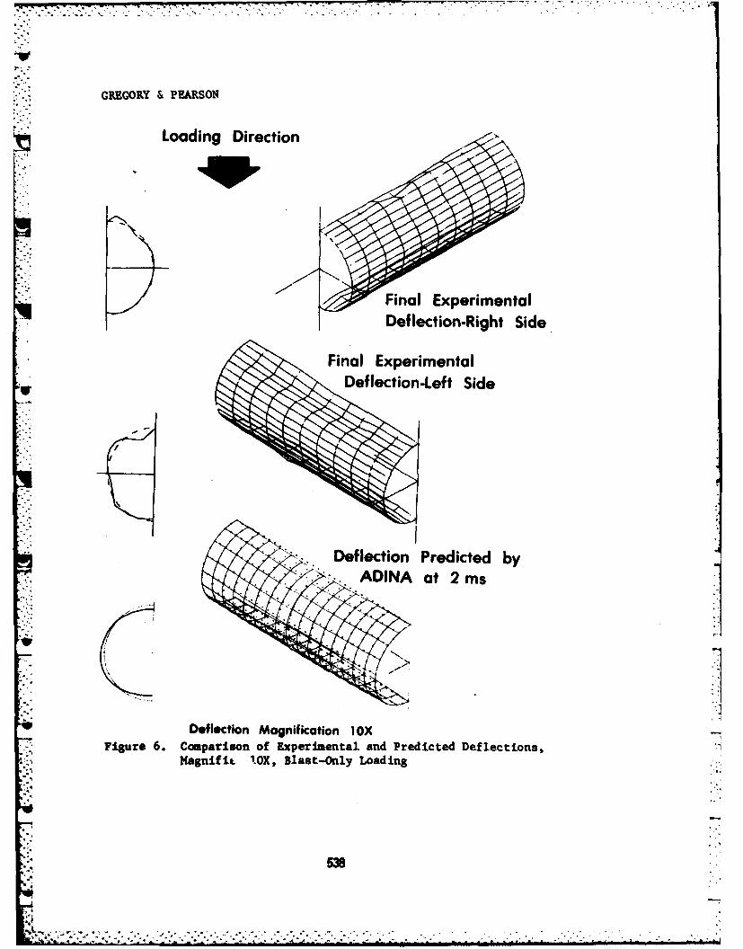
-v
GREGORY & PEARSON
Loading Direction
Final ExperimentalDeflection-Right Side
Final ExperimentalDeflection-Left Side
II
SDef lection Predicted byAD-N at 2 ms
Deflection Magnification IOXFigure 6. Comparison of Experimental and Predicted Deflections,
Magnific IOX, Blast-Only Loading
? , ..-8
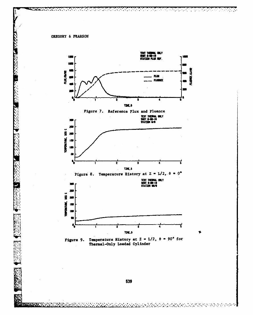
GREGORY & PEARSON
r IBTR 1MMttL OL&94IST in.ML
WAIF= " W.
- - - -,- - - - - -
a , ..., . , ....
Figure 7. Reference Flux and Fluence
": : TnST nar L SLY
STATION SS
So
I
.44
Figure 8. Temperature History at Z 0 L2,.TT AIl. OLY
3S0OT Se O-ISSTATION W
UK'
I
Figure 9. Temperature History at Z - L/2, 8 - 90 for
Thermal-Only Loaded Cylinder
ig 539
, . ;: ', :; : ,:.i ':,'.t'.,, .. '::._". ' :.'........ S, , ,_' .,'',...'""'','" . _ , . .
P
GREGORY & PEARSON
Measurements on the post-test thermally loaded cylinder showed aslight degree of buckling near the end of the cylinder on the near side.The deformation pattern is shown In the top two subplots of Figure 10 andis nearly symmetric in both the Z and 0 coordinates. The displacementsfrom the original geometric positions are magnifled by lOX in Figure 10.The deflection was small and was most apparent to the unaided eye near eachend where the largest changes in slope occurred. The deformation crosssections at the mid-point, Z - L/2, are shown on the left side of Figure 10.The displacement was outward at 8 - 0* and inward at 0 - 90*.
The ADINA simulation of the thermally loaded cylinder was carried outto 1.1 ms. Plasticity occurred early in the calculation and peak deflec-
K, tions were observed at approximately 0.725 is. The deformed shape at thistime as predicted by ADIMA is shown in the lower part of Figure 10. Theapparent cut shown in Figure 10 at Z - L/2 Is the prescribed constantZ-displacement which simulates the thermal expansion. The prescribed dis-placement ranged from 1.8 am at 0 - o to zero at 0 - 120'. The deforms-tion cross section at Z - L/2 showed a similar trend as did the experi-mental results. However, no buckling was predicted by ADINA near theZ - L/20 point, contrary to what was observed in the experiment. An incip-ient buckling deflection of approximately twice the cylinder thicknessappeared to be forming at Z - L/2, 0 a 100" in the ADINA results.
In the final test in the BIL Thermal/Blast Simulator, the cylinderwas exposed to the thermal radiation, rotated and exposed to the air shock.The reference flux and temperature histories at 0* and 90* are shown inFigures 11-13. The long term stagnation pressure record is shown inFigure 14. The pressure loadings on the cylinder at e - 00 and 90* areshown in Figure 15 and 16. Comparing Figures 15 and 16 with Figures 4 and5, one notices that the pressure load rises much more gradually in thepresence of the heated air surrounding the cylinder. From Figures 14 and3, one sees that the long term pressure produced by the shock tube is onlyslightly less for the thermal/blast test than was the case for the blast-only test. As shnwn in Figures 12 and 8, the peak temperature rise inthermal/blast test was 1700C and in the thermal-only test it was 225*C.
The final deformed shape of the cylinder after the combined thermal/blast test is shown in Figure 17. The deformation is symmetric with re-spect to the two symmetry planes. The deflection magnification in Figure17 Is only 5X, one half of the magnification used in Figures 6 and 10. At.Z - L/2, the peak radial deflection for the thermal/blast test is approxi-mately 4 tines as large as for the blast-only deflection and 10 times aslarge as the thermal-only deflection. ADINA calculations for the thermal/blast simulation have not been made and no comparisons are available.
S*~ ' - * t *'** . . . . * .*-'
GREGORY & PEARSON
Loading Direction '
Final ExperimentalDeflection-Right Side
Final Experimental
Deflection-Left Side
Deflection Predicted byADINA at 0.725 ms
Dofhcfon Magnifcation IOXFlure 10. Comparison of Experimental and Predicted Deflections,
Magnifiled lOX, Thermal-Only Loading
541
GREGORY & PEARSON
MUT UMLWVT=l FLUX FR.
- - - - - - - -
a,2 3 4
'Figure 11. Thermal/Blast Test, Reference Flux and Fluence
m am 41-I$TAT=I W14.5
m7
Figure 12. Thermal/Blast Test, Temperature History at Z -L/10, 0 - *
lET UNALMT
454
jGREGRY &PEARSON
RtAI= am. aw.
Figure 14. Thermal/Blast Test, Read-On Pressure
4..8
21 4 6 61i
Figure 15. Thermal/Blast Test, Diffraction Phase Loading at 0O
UTWI: U EVLK
Figure 16. Thermal/Blast Test, Diffraction Phase Loading at 900
643
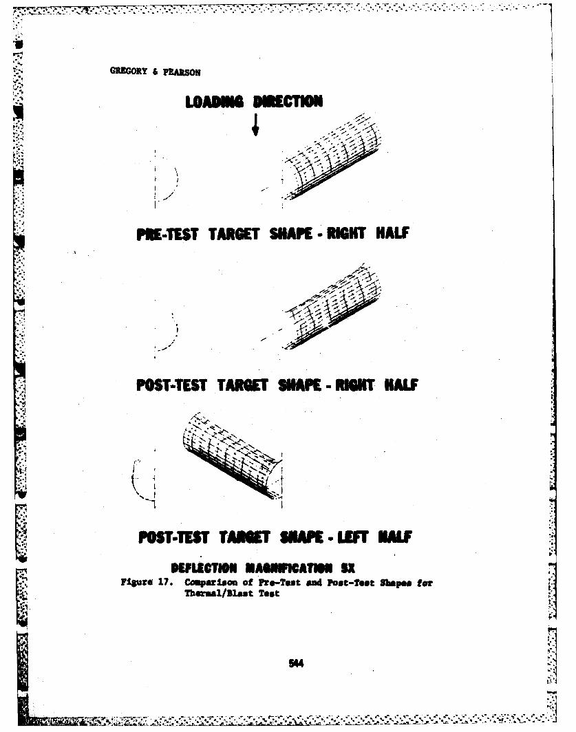
GREGORY & PEARSON
c.
LOAMBUTO
M..
NE-ThET TARGETestAE.RGTHL
544C
GREGORY & PEARSON
CONCLUSIONS
The series of tests showed that the effect of combined thermal andblast loadings at realistic time separations produces a nonlinear responsein thermally thin targets. Moreover, the shape of the deformed cylindersIs markedly different between the three tests. The heated cylinder tended
to displace outward on the near and far sides; whereas, the combined testresulted in a dished-in surface on the near side.
The results obtained thus far with ADINA are not as satisfying as wasoriginally expected. However, the permanent deflections produced in boththe thermal-only and blast-only tests were very small. Furthermore, thegeneral shape of the deformations predicted by ADINA was correct. It isevident that we need to develop a Kirchhoff shell element whose stabletime step is not limited by the rotatory inertia. This would improve theefficiency of the ADINA calculation significantly.
REFERENCES
1. P. J. Morris, "A Review of Research on Thermal Radiation Degradation ofStructural Resistance to Air Blast," (U), URS Research Company, DNA-2856F, December 1971 (SECRET).
2. D. N. Wilson, "The Distribution and History of Temperature in CircularCylinders Exposed to the Thermal Radiation Pulse of a Nuclear Deto-nation," NOLTR-71-61, June 1971.
3. R. J. Pearson, et al, "Synergism in Nuclear Thermal/Blast Loading,"Seventh International Symposium on Military Applications of BlastSimulation, Medicine Hat, Alberta, Canada, July 1981.
4. K. J. Bathe, "ADINA, A Finite Element Program for Automatic DynamicIncremental Analysis," MIT-82448-1, December 1978.
4.1 5. T. Stefansky, et al, "Temperature Induced Degradation of MechanicalProperties Following Instantaneous Heating," AFWL-TR-71-62, Sep 1977.
6. K. J. Bathe, "ADINAT, A Finite Element Program for the AutomaticDynamic Incremental Nonlinear Analysis of Temperatures," MIT-82448-5,Dec. 1978.
qw.s. .. aW rsuut= WrIca I,,-54a-uWjn, 5
.....................................