A D E D & C A D P P - Department of Computer Science

Automatic Discovery of

Efficient Divide-&-Conqer Algorithms for

Dynamic Programming Problems

Pramod Ganapathi

A Dissertation presented to the faculty of Stony Brook University

in partial fulfillment of the requirements for the degree ofDoctor of Philosophy in the field of Computer Science

specializing in Algorithms

Advisor: Rezaul Chowdhury

Dec 2016

Automatic Discovery of

Efficient Divide-&-Conqer Algorithms for

Dynamic Programming Problems

Pramod Ganapathi

Dissertation Committee:

Rezaul Chowdhury, Stony Brook University

Michael A. Bender, Stony Brook University

Yanhong A. Liu, Stony Brook University

Barbara Chapman, Stony Brook University

Kunal Agrawal, Washington University

Dedicated to mathematics, puzzles, algorithms, & philosophy.

Acknowledgments

Many lives are directly or indirectly responsible for this 3.5 year work and for my amazingPh.D. life. In this small section, I would like to express my sincere and heartful gratitudeto all of them.

First and foremost, I thank this enigmatic cosmos for everything. I thank my biologicalparents – (mother) Varada and (father) Ganapathi Hegde for their love, care, and affec-tion and for their sacrifice in bringing me up; and all my wonderful relatives, especially(older brother) Prashanth Hegde, (paternal uncle) Hegde Jadugar, (cousin) Sudha Hegde,and (cousin) Shobha Hegde, for always showering love upon me. Most importantly, I thankthe lady I loved, for introducing me to the world of beauty, love, dreams, imagination, andaddiction. I am infinitely indebted to that Goddess for the eternal happiness and uncondi-tional love she has given to me. I also thank my closest friend Darshan S. Palasamudramfor countless hours of brain-drilling philosophical discussions and ground-breaking analy-ses on hundreds of topics.

From the bottom of my heart, I would like to thank my research guru, my algorithmsteacher, my great advisor, and the superhero of my Ph.D. life – Rezaul Chowdhury, forintroducing me to the world of organized research and rigorous algorithmic thinking. Hestressed importance on novelty, technicality, mathematical rigorousness, presentation, andacademic integrity. He taught me that a world of problems is in fact a world of opportu-nities because with each problem there comes an opportunity to solve the problem. Myproblem-solving ability has increased tremendously under his tutelage.

Rezaul is the reason for my transformational thinking from “The given problem is im-possible to solve” to “There must be a very simple solution to the given problem and I willfind that solution in 3 days”. In the initial years of my Ph.D., I viewed problems as lionsand myself as a deer whose only goal was to run away from the lions and survive. In thefinal years of my Ph.D., I saw myself as a powerful lion and problems as deers and my onlyaim was to attack and nail the deers down one-by-one. In this way, Rezaul rewired mybelief system.

I am eternally grateful to Rezaul for having given me a diamond opportunity to designAutogen (an algorithm to discover other algorithms), which is the greatest computer algo-rithm I have ever (co-)designed, which now forms the core of my Ph.D. dissertation. Rezaulgave me a beautiful opportunity to lead and advise 8 master’s and 2 undergrad students fortheir research projects. He gave me a lot of freedom to choose the problems I like and takeas much time as necessary to solve them. I thank Rezaul in a non-terminating recursiveloop for everything he has taught me.

I thank my algorithms teacher Michael A. Bender for exponentially increasing my love

iv

towards algorithms in general and dynamic programming in specific, through his leg-endary classes on graduate algorithms. Michael taught me great presentation and cool-ness and boosted my confidence to a very high level. Michael’s simplicity and humblenessis unparalleled. Thanks to Himanshu Gupta, who taught me the theory of database sys-tems, in which I learned several beautiful I/O-efficient algorithms. I also thank Joseph S.B. Mitchell for teaching me computational geometry and always inspiring me through hisdynamic personality. Many thanks to Steven Skiena for advice. Thanks to Yanhong A. Liu,Barbara Chapman, and Kunal Agrawal for their encouragement. Thanks also due to I. V.Ramakrishnan for support.

I thank my mother-country India for teaching me the greatness of simplicity and thepower of teaching. I thank my father-country United States of America for teaching me thegreatness of positive thinking and the power of learning. I sincerely thank the great math-ematics teachers of my school and college: Shanthakumari, Vathsala, Shridhar, Prasad,A. V. Shiva Kumar, P. C. Nagaraj, K. S. Anil, and C. Chamaraju for making me desperateto learn mathematics and appreciate the beauty of this sexy queen. I thank my favoriteschool teacher Veena who encouraged my attitude of questioning everything. I also thankthe author Anany Levitin for introducing me to my girlfriend – algorithms, and makingme algoholic through his classic textbook on algorithms. Thanks also to my two greatundergrad computer science teachers: Udaya and Shilpa B. V., for having taught me pro-gramming, data structures, and algorithms with so much passion. I am also extremelygrateful to my mentors at IBM: Sanjay M. Kesavan, Lohitashwa Thyagaraj, and AmruthaPrabhu for training me to become a good leader.

I wholeheartedly thank all the greatest books I have studied on mathematics, puzzles,algorithms, and philosophy that have heavily influenced the way I think and solve prob-lems. In particular, I am eternally grateful to the greatest book I have ever studied – ThePower of Your Subconscious Mind by Joseph Murphy. The terrific book has injected in myblood and mind the unshakable thought that whatever I believe becomes reality. I am alsoextremely thankful to the great movies and TV series I have watched, which have signifi-cantly influenced my mental personality and thinking. I would like to thank all resourcesthat have taught me something or the other.

Thanks due to Jackson Menezes, Abhiram Natarajan, Pramodh Nataraj, Anil Bhandary,and Pradeep S. Bhat for all the brainstorming discussions on puzzles, algorithms, and phi-losophy. I founded an organization called Stony Brook Puzzle Society (SBPS) and taughtthe art of nailing mathematical, algorithmic, and logic puzzles to Ph.D., master’s, and un-dergrad students for 3 years. Thanks to my favorite SBPS students: Rong Zou, AndreyGorlin, Quan Xie, Sourabh Daptardar, and Tom Duplessis for teaching me different waysto attack puzzles and also for assuring me that there are still a few people in the worldwho genuinely love classic mathematical puzzles.

I thank my colleagues: Jesmin Jahan Tithi – for high-performing implementations andoptimizations of several 2-way divide-and-conquer algorithms and also for the brainstorm-ing discussion that led to the discovery of divide-and-conquer CYK algorithm; Vivek Prad-han – for two nice brainstorming sessions in which we discovered the first cache-efficientcache-oblivious Viterbi algorithm; Stephen Tschudi, the super-jet programmer – for fastand extraordinary implementations of r-way divide-and-conquer algorithms on GPUs andalso for implementing the deductive Autogen algorithm; Samuel McCauley – for several

v

nice discussions on the spherical range 1 query (R1Q) problem; Rathish Das – for the imple-mentations of GPU algorithms in external-memory; Dhruv Matani – for a discussion thatled to a linear-space (in bits) complexity proof of d-D orthogonal R1Q algorithm; YunpengXiao – for the implementation of the multi-instance Viterbi algorithm; Arun Rathakrish-nan – for discussions to develop a divide-and-conquer protein accordion folding algorithm;Mohammad Mahdi Javanmard, Premadurga Kolli, and Isha Khanna – for discussions andimplementations for space-parallelism tradeoff of divide-and-conquer algorithms; Anshuland Nitish Garg – for discussions on a few task schedulers which led to the design of a(space-inefficient) recursive wavefront algorithm scheduler; and Matthew Fleishman andCharles Bachmeier – for extending my Autogen implementation.

My work was funded by the National Science Foundation (NSF) grants: CCF-1162196,CCF-1439084, and CNS-1553510. I thank Cynthia SantaCruz-Scalzo (or Cindy), the mostlovely graduate student service secretary ever, for her invaluable help for all my documen-tation and paperwork. I thank the Institute of Advanced Computational Science (IACS)for giving me a wonderful workspace. I also thank Sarena Romano, the sweet IACS traveland event coordinator for being so nice whenever I needed help.

My lovely American family: Susan, Carlo, and their son John Colatosti deserve a spe-cial thanks for treating me as a member of their own family and for their continuous loveand affection. My mom Susan exposed me to the American culture, took me to severalwonderful places in Long Island, and taught me the ways of appreciating the beauty ofnature, experiencing life, and being grateful for the blessings in life. The long bike rides,breakfasts at Port Jefferson, church visits, frequent dinners, walks on the shore of WestMeadow beach, and camping at Smith Point beach, all these experiences with Susan nowseek existence only in my memories. I thank my another American family: Pamela andFrank Murphy for their love and affection. Pamela and I shared a lot of common interestssuch as good conversations, photography, nature, arts, and so on. I thank her for beingso nice and always caring. Thanks to my close roommates: Ayon Chakraborty, ChiragMandot, and Franklin George in celebrating life with chit-chats, tasty food, discussions,arguments, drink parties, pranks, dances, and beach trips. Thanks to Pavithra K. Srinathand Pallavi Ghosh for their support and encouragement; and several other friends for allmemorable fun moments. I am also extremely thankful to the West Meadow beach, mymost favorite location near Stony Brook, where I have spent an uncountable number ofromantic evenings watching the sunset and contemplating on the deeper meanings of life,love, and the world.

Finally, I wish to thank everything in this aesthetically beautiful and enigmatic cosmosthat is directly or indirectly responsible for this work and my mind-blowingly-awesome life.

Pramod Ganapathi

Stony Brook, USADecember 2016

vi

Abstract

This dissertation is an excursion into computer-discovered algorithms and computer-aidedalgorithm design. In our vision of the not-so-distant future of computing, machines willtake the responsibility of designing and implementing most, if not all, machine-specifichighly efficient nontrivial algorithms with provable correctness and performance guaran-tees. Indeed, as the complexity of computing hardware grows and their basic architectureskeep changing rapidly, manually redesigning and reimplementing key algorithms for highperformance on every new architecture is quickly becoming an impossible task. Automa-tion is needed.

We design algorithms that can design other algorithms. Our focus is on auto-generatingalgorithms for solving dynamic programming (DP) recurrences efficiently on state-of-the-art parallel computing hardware. While DP recurrences can be solved very easily usingnested or even tiled nested loops, for high performance on modern processors/coprocessorswith cache hierarchies, portability across machines, and automatic adaptivity to runtimefluctuations in the availability of shared resources (e.g., cache space) highly nontrivialrecursive divide-and-conquer algorithms are needed. But, these recursive divide-and-conquer algorithms are difficult to design and notoriously hard to implement for high per-formance. Furthermore, new DP recurrences are being encountered by scientists everyday for solving brand new problems in diverse application areas ranging from economics tocomputational biology. But, how does an economist or a biologist without any formal train-ing in computer science design an efficient algorithm for evaluating his/her DP recurrenceon a computer? Well, we can help!

We present Autogen – an algorithm that given any blackbox implementation of a DPrecurrence (e.g., inefficient naive serial loops) from a wide class of DP problems, can auto-matically discover a fast recursive divide-and-conquer algorithm for solving that problemon a shared-memory multicore machine. We mathematically formalize Autogen, prove itscorrectness, and provide theoretical performance guarantees for the auto-discovered algo-rithms. These auto-generated algorithms are shown to be efficient (e.g., highly parallelwith highly optimizable kernels, and cache-, energy-, and bandwidth-efficient), portable(i.e., cache- and processor-oblivious), and robust (i.e., cache- and processor-adaptive).

We present Autogen-Wave – a framework for computer-assisted discovery of fast divide-and-conquer wavefront versions of the algorithms already generated by Autogen. These re-cursive wavefront algorithms retain all advantages of the Autogen-discovered algorithmson which they are based, but have better and near-optimal parallelism due to the wave-front order of execution. We also show how to schedule these algorithms with provableperformance guarantees on multicore machines.

We present Viterbi – an efficient cache-oblivious parallel algorithm to solve the Viterbirecurrence, as a first step toward extending Autogen to handle DP recurrences with ir-

vii

regular data-dependent dependencies. Our algorithm beats the current fastest Viterbialgorithm in both theory and practice.

We present Autogen-Fractile – a framework for computer-aided design of high-performingand easily portable recursively tiled/blocked algorithms for a wide class of DP problemshaving fractal-type dependencies. These recursively tiled algorithms have excellent cachelocality and excellent parallel running time on multi-/many-core machines with deep mem-ory hierarchy.

We present Autogen-Tradeoff – a framework that can be used to design efficient andportable not-in-place algorithms to asymptotically increase the parallelism of some of theAutogen-discovered algorithms without affecting cache-efficiency.

This dissertation takes the first major step on which to build computing systems forautomatically designing efficient and portable nontrivial algorithms. We hope that morework follows in this science of algorithm discovery.

viii

Contents

Acknowledgments iv

Abstract vii

1 Introduction & Background 11.1 Motivation and vision . . . . . . . . . . . . . . . . . . . . . . . . . . . . . . . . . 11.2 Cache-efficient algorithms . . . . . . . . . . . . . . . . . . . . . . . . . . . . . . 2

1.2.1 I/O model . . . . . . . . . . . . . . . . . . . . . . . . . . . . . . . . . . . . 31.2.2 Cache-oblivious model . . . . . . . . . . . . . . . . . . . . . . . . . . . . 41.2.3 Parallel cache-oblivious model . . . . . . . . . . . . . . . . . . . . . . . . 4

1.3 Cache-oblivious algorithms . . . . . . . . . . . . . . . . . . . . . . . . . . . . . 51.4 Parallel algorithms . . . . . . . . . . . . . . . . . . . . . . . . . . . . . . . . . . 6

1.4.1 Dynamic multithreading model . . . . . . . . . . . . . . . . . . . . . . . 61.4.2 Parallel memory hierarchy model . . . . . . . . . . . . . . . . . . . . . . 71.4.3 Parallel algorithms . . . . . . . . . . . . . . . . . . . . . . . . . . . . . . 8

1.5 Scheduling algorithms . . . . . . . . . . . . . . . . . . . . . . . . . . . . . . . . 91.5.1 Greedy scheduler . . . . . . . . . . . . . . . . . . . . . . . . . . . . . . . 91.5.2 Parallel depth first scheduler . . . . . . . . . . . . . . . . . . . . . . . . 91.5.3 Work-stealing scheduler . . . . . . . . . . . . . . . . . . . . . . . . . . . 101.5.4 Space-bound scheduler . . . . . . . . . . . . . . . . . . . . . . . . . . . . 11

1.6 Algorithm design techniques . . . . . . . . . . . . . . . . . . . . . . . . . . . . . 111.6.1 Divide-and-conquer . . . . . . . . . . . . . . . . . . . . . . . . . . . . . . 121.6.2 Dynamic programming (DP) . . . . . . . . . . . . . . . . . . . . . . . . . 121.6.3 Divide-and-conquer dynamic programming . . . . . . . . . . . . . . . . 14

1.7 Dynamic programming implementations . . . . . . . . . . . . . . . . . . . . . 141.7.1 Iterative DP algorithms . . . . . . . . . . . . . . . . . . . . . . . . . . . 151.7.2 Blocked / tiled iterative DP algorithms . . . . . . . . . . . . . . . . . . . 151.7.3 Recursive divide-and-conquer DP algorithms . . . . . . . . . . . . . . . 16

1.8 Automatic algorithm discovery . . . . . . . . . . . . . . . . . . . . . . . . . . . 161.8.1 Program synthesis . . . . . . . . . . . . . . . . . . . . . . . . . . . . . . 171.8.2 Polyhedral compilers . . . . . . . . . . . . . . . . . . . . . . . . . . . . . 17

1.9 Dissertation outline . . . . . . . . . . . . . . . . . . . . . . . . . . . . . . . . . . 181.9.1 Dissertation statement . . . . . . . . . . . . . . . . . . . . . . . . . . . . 181.9.2 Dissertation contributions . . . . . . . . . . . . . . . . . . . . . . . . . . 181.9.3 Dissertation organization . . . . . . . . . . . . . . . . . . . . . . . . . . 20

ix

2 Automatic Discovery of Efficient Divide-&-Conquer DP Algorithms 222.1 Introduction . . . . . . . . . . . . . . . . . . . . . . . . . . . . . . . . . . . . . . 222.2 The Autogen algorithm . . . . . . . . . . . . . . . . . . . . . . . . . . . . . . . . 27

2.2.1 Cell-set generation . . . . . . . . . . . . . . . . . . . . . . . . . . . . . . 292.2.2 Algorithm-tree construction . . . . . . . . . . . . . . . . . . . . . . . . . 302.2.3 Algorithm-tree labeling . . . . . . . . . . . . . . . . . . . . . . . . . . . . 312.2.4 Algorithm-DAG construction . . . . . . . . . . . . . . . . . . . . . . . . 33

2.3 Correctness of Autogen . . . . . . . . . . . . . . . . . . . . . . . . . . . . . . . . 342.3.1 Threshold problem size . . . . . . . . . . . . . . . . . . . . . . . . . . . . 342.3.2 The Fractal-dp class . . . . . . . . . . . . . . . . . . . . . . . . . . . . . 352.3.3 Proof of correctness . . . . . . . . . . . . . . . . . . . . . . . . . . . . . . 37

2.4 Complexity analysis . . . . . . . . . . . . . . . . . . . . . . . . . . . . . . . . . . 392.4.1 Space/time complexity of Autogen . . . . . . . . . . . . . . . . . . . . . 402.4.2 Cache complexity of an R-DP . . . . . . . . . . . . . . . . . . . . . . . . 402.4.3 Upper-triangular system of recurrence relations . . . . . . . . . . . . . 41

2.5 Extensions of Autogen . . . . . . . . . . . . . . . . . . . . . . . . . . . . . . . . 432.5.1 One-way sweep property violation . . . . . . . . . . . . . . . . . . . . . 442.5.2 Space reduction . . . . . . . . . . . . . . . . . . . . . . . . . . . . . . . . 452.5.3 Non-orthogonal regions . . . . . . . . . . . . . . . . . . . . . . . . . . . . 46

2.6 The deductive Autogen algorithm . . . . . . . . . . . . . . . . . . . . . . . . . . 472.6.1 Generic iterative algorithm construction . . . . . . . . . . . . . . . . . . 482.6.2 Algorithm-tree construction . . . . . . . . . . . . . . . . . . . . . . . . . 502.6.3 Space/time complexity of deductive Autogen . . . . . . . . . . . . . . . 51

2.7 Experimental results . . . . . . . . . . . . . . . . . . . . . . . . . . . . . . . . . 522.7.1 Experimental setup . . . . . . . . . . . . . . . . . . . . . . . . . . . . . . 522.7.2 Single-process performance . . . . . . . . . . . . . . . . . . . . . . . . . 552.7.3 Multi-process performance . . . . . . . . . . . . . . . . . . . . . . . . . . 55

2.8 Conclusion and open problems . . . . . . . . . . . . . . . . . . . . . . . . . . . . 58

3 Semi-Automatic Discovery of Efficient Divide-&-Conquer Wavefront DP Al-gorithms 603.1 Introduction . . . . . . . . . . . . . . . . . . . . . . . . . . . . . . . . . . . . . . 603.2 The Autogen-Wave framework . . . . . . . . . . . . . . . . . . . . . . . . . . . . 66

3.2.1 Completion-time function construction . . . . . . . . . . . . . . . . . . . 693.2.2 Start-time and end-time functions construction . . . . . . . . . . . . . 713.2.3 Divide-and-conquer wavefront algorithm derivation . . . . . . . . . . . 73

3.3 Correctness . . . . . . . . . . . . . . . . . . . . . . . . . . . . . . . . . . . . . . . 743.4 Scheduling algorithms . . . . . . . . . . . . . . . . . . . . . . . . . . . . . . . . 75

3.4.1 Work-stealing scheduler . . . . . . . . . . . . . . . . . . . . . . . . . . . 773.4.2 Modified space-bounded scheduler . . . . . . . . . . . . . . . . . . . . . 79

3.5 Further improvement of parallelism . . . . . . . . . . . . . . . . . . . . . . . . 823.6 Experimental results . . . . . . . . . . . . . . . . . . . . . . . . . . . . . . . . . 83

3.6.1 Projected parallelism . . . . . . . . . . . . . . . . . . . . . . . . . . . . . 833.6.2 Running time and cache performance . . . . . . . . . . . . . . . . . . . 84


x

4 An Efficient Divide-&-Conquer Viterbi Algorithm 874.1 Introduction . . . . . . . . . . . . . . . . . . . . . . . . . . . . . . . . . . . . . . 874.2 Cache-inefficient Viterbi algorithm . . . . . . . . . . . . . . . . . . . . . . . . . 884.3 Cache-efficient multi-instance Viterbi algorithm . . . . . . . . . . . . . . . . . 924.4 Viterbi algorithm using rank convergence . . . . . . . . . . . . . . . . . . . . . 94

4.4.1 Original algorithm . . . . . . . . . . . . . . . . . . . . . . . . . . . . . . 944.4.2 Improved algorithm . . . . . . . . . . . . . . . . . . . . . . . . . . . . . . 95

4.5 Cache-efficient Viterbi algorithm . . . . . . . . . . . . . . . . . . . . . . . . . . 974.6 Lower bound . . . . . . . . . . . . . . . . . . . . . . . . . . . . . . . . . . . . . . 994.7 Experimental results . . . . . . . . . . . . . . . . . . . . . . . . . . . . . . . . . 100

4.7.1 Multi-instance Viterbi algorithm . . . . . . . . . . . . . . . . . . . . . . 1014.7.2 Single-instance Viterbi algorithm . . . . . . . . . . . . . . . . . . . . . . 101


5 Semi-Automatic Discovery of Efficient Divide-&-Conquer Tiled DP Algo-rithms 1045.1 Introduction . . . . . . . . . . . . . . . . . . . . . . . . . . . . . . . . . . . . . . 1055.2 r-way R-DP algorithms . . . . . . . . . . . . . . . . . . . . . . . . . . . . . . . . 109

5.2.1 Importance of r-way R-DPs . . . . . . . . . . . . . . . . . . . . . . . . . 1095.2.2 Types of r-way R-DPs . . . . . . . . . . . . . . . . . . . . . . . . . . . . 1105.2.3 GPU computing model . . . . . . . . . . . . . . . . . . . . . . . . . . . . 110

5.3 The Autogen-Fractile framework . . . . . . . . . . . . . . . . . . . . . . . . . . 1115.3.1 Approach 1: Generalization of 2-way R-DP . . . . . . . . . . . . . . . . 1115.3.2 Approach 2: Generalization of parallel iterative base cases . . . . . . . 116

5.4 Complexity analysis . . . . . . . . . . . . . . . . . . . . . . . . . . . . . . . . . . 1195.4.1 I/O complexity . . . . . . . . . . . . . . . . . . . . . . . . . . . . . . . . . 1195.4.2 Parallel running time . . . . . . . . . . . . . . . . . . . . . . . . . . . . . 121

5.5 Experimental results . . . . . . . . . . . . . . . . . . . . . . . . . . . . . . . . . 1235.5.1 Experimental setup . . . . . . . . . . . . . . . . . . . . . . . . . . . . . . 1235.5.2 Internal-memory GPU implementations . . . . . . . . . . . . . . . . . . 1235.5.3 External-memory GPU implementations . . . . . . . . . . . . . . . . . 125


6 Semi-Automatic Discovery of Divide-&-Conquer DP Algorithms with Space-Parallelism Tradeoff 1286.1 Introduction . . . . . . . . . . . . . . . . . . . . . . . . . . . . . . . . . . . . . . 1286.2 The Autogen-Tradeoff framework . . . . . . . . . . . . . . . . . . . . . . . . . 132

6.2.1 In-place algorithm construction . . . . . . . . . . . . . . . . . . . . . . . 1326.2.2 Span analysis . . . . . . . . . . . . . . . . . . . . . . . . . . . . . . . . . 1336.2.3 Not-in-place algorithm construction . . . . . . . . . . . . . . . . . . . . 1346.2.4 Hybrid algorithm construction . . . . . . . . . . . . . . . . . . . . . . . 135

6.3 Experimental results . . . . . . . . . . . . . . . . . . . . . . . . . . . . . . . . . 1376.4 Conclusion and open problems . . . . . . . . . . . . . . . . . . . . . . . . . . . . 137

xi

A Efficient Divide-&-Conquer DP Algorithms 139A.1 Longest common subsequence & edit distance . . . . . . . . . . . . . . . . . . 139A.2 Parenthesis problem . . . . . . . . . . . . . . . . . . . . . . . . . . . . . . . . . 143A.3 Floyd-Warshall’s all-pairs shortest path . . . . . . . . . . . . . . . . . . . . . . 152A.4 Gaussian elimination without pivoting . . . . . . . . . . . . . . . . . . . . . . . 157A.5 Sequence alignment with gap penalty . . . . . . . . . . . . . . . . . . . . . . . 161A.6 Protein accordion folding . . . . . . . . . . . . . . . . . . . . . . . . . . . . . . . 164A.7 Function approximation . . . . . . . . . . . . . . . . . . . . . . . . . . . . . . . 167A.8 Spoken word recognition . . . . . . . . . . . . . . . . . . . . . . . . . . . . . . . 171A.9 Bitonic traveling salesman . . . . . . . . . . . . . . . . . . . . . . . . . . . . . . 173A.10 Cocke-Younger-Kasami algorithm . . . . . . . . . . . . . . . . . . . . . . . . . . 175A.11 Binomial coefficient . . . . . . . . . . . . . . . . . . . . . . . . . . . . . . . . . . 176A.12 Egg dropping . . . . . . . . . . . . . . . . . . . . . . . . . . . . . . . . . . . . . . 179A.13 Sorting algorithms . . . . . . . . . . . . . . . . . . . . . . . . . . . . . . . . . . 181

A.13.1 Bubble sort . . . . . . . . . . . . . . . . . . . . . . . . . . . . . . . . . . . 186A.13.2 Selection sort . . . . . . . . . . . . . . . . . . . . . . . . . . . . . . . . . 189A.13.3 Insertion sort . . . . . . . . . . . . . . . . . . . . . . . . . . . . . . . . . 190A.13.4 Experimental results . . . . . . . . . . . . . . . . . . . . . . . . . . . . . 193

A.14 Conclusion and open problems . . . . . . . . . . . . . . . . . . . . . . . . . . . . 195

B Efficient Divide-&-Conquer Wavefront DP Algorithms 197B.1 Matrix multiplication . . . . . . . . . . . . . . . . . . . . . . . . . . . . . . . . . 197B.2 Longest common subsequence & edit distance . . . . . . . . . . . . . . . . . . 197B.3 Floyd-Warshall’s all-pairs shortest path . . . . . . . . . . . . . . . . . . . . . . 199B.4 Sequence alignment with gap penalty . . . . . . . . . . . . . . . . . . . . . . . 199

C Efficient Divide-&-Conquer DP Algorithms for Irregular Problems 203C.1 Sieve of Eratosthenes . . . . . . . . . . . . . . . . . . . . . . . . . . . . . . . . . 203C.2 Knapsack problem . . . . . . . . . . . . . . . . . . . . . . . . . . . . . . . . . . . 210

D Efficient Divide-&-Conquer Tiled DP Algorithms 220D.1 Matrix multiplication . . . . . . . . . . . . . . . . . . . . . . . . . . . . . . . . . 220D.2 Longest common subsequence . . . . . . . . . . . . . . . . . . . . . . . . . . . . 220D.3 Floyd-Warshall’s all-pairs shortest path . . . . . . . . . . . . . . . . . . . . . . 220D.4 Gaussian elimination without pivoting . . . . . . . . . . . . . . . . . . . . . . . 221D.5 Parenthesis problem . . . . . . . . . . . . . . . . . . . . . . . . . . . . . . . . . 221D.6 Sequence alignment with gap penalty . . . . . . . . . . . . . . . . . . . . . . . 222

E Efficient Divide-&-Conquer Hybrid DP Algorithms 224E.1 Matrix multiplication . . . . . . . . . . . . . . . . . . . . . . . . . . . . . . . . . 224E.2 Multi-instance Viterbi algorithm . . . . . . . . . . . . . . . . . . . . . . . . . . 225E.3 Floyd-Warshall’s all-pairs shortest path . . . . . . . . . . . . . . . . . . . . . . 226E.4 Protein accordion folding . . . . . . . . . . . . . . . . . . . . . . . . . . . . . . . 228

xii

Chapter 1

Introduction & Background

“All life is problem-solving”, says Karl Popper, a famous philosopher. Considering problem-solving itself as a problem, can we solve the problem of problem-solving? In the world ofcomputer science, problem-solving often means coming up with algorithms to solve com-puter science problems. Solving the problem of problem-solving means coming up withan algorithm that can automatically come up with various other algorithms for solving amultitude of problems. In this dissertation, we answer affirmatively that we can solve theproblem of problem-solving for a class of problems by designing algorithms / frameworksthat can automatically / semi-automatically discover other efficient and portable nontrivialalgorithms to solve a wide class of dynamic programming problems.

1.1 Motivation and visionProgramming is hard. Programming typically involves understanding the given problemdeeply, identifying / coming up with data structures to structure and organize the data,finding provably correct algorithms for solving the problem that access data from the datastructures efficiently, and coding the algorithms and data structures to take the problemspecification as input and output the desired solutions. Performance is usually the mostimportant measure of goodness of correct programs. In computer science, almost all pathslead not to Rome but to develop high-performing programs.

A majority of today’s algorithms are sequential. Each step of execution of a serial algo-rithm consists of an instruction. The speed of the sequential computers has improved expo-nentially for several years through increase in the number of transistors on an integratedcircuit. The improvement is now coming at very high costs. As a result, manufacturersare building parallel computers with multiple processing elements which are cost-effectiveand also improve the total computing speed. To solve problems on parallel computers effi-ciently, we need to design parallel algorithms and each step of execution in such algorithmsconsists of multiple instructions.

Real-life applications [Chen et al., 2014] [Kim et al., 2014] such as databases (of Google,Facebook, Microsoft, Twitter, Netflix, IBM, Amazon, etc), cryptography, computer graph-ics, computer vision, weather forecasting, crystallography, simulation of galaxy formationand planetary movements, gene analysis, material science, circuit design, defense, geology,molecular science, condensed matter, etc involve gigantic volume of computations whichwhen executed sequentially might take months to years. Parallelism is one of the key

1

factors in improving performance. Hence, designing parallel algorithms typically leads tohigh-performing programs.

Modern computers have a tree-like hierarchy of caches having different sizes and accesstimes. A typical algorithm has to access data and when the data does not fit in a partic-ular cache it moves back-and-forth between different levels of caches. Reducing the totalnumber of such data transfers improves the overall performance. Cache locality is yet an-other key factor to improve performance. Hence, designing cache-efficient algorithms (i.e.,algorithms with good cache locality) might lead to more efficient programs.

Most of today’s cache-efficient parallel algorithms are cache-aware and/or processor-aware. This means the algorithms need to know the machine parameters such as cachesize, block size, number of levels of caches, number of processors etc. There are severaltypes of machine architectures and it is not feasible to write cache-efficient parallel pro-grams for every single one of them. Resource-obliviousness (e.g: processor- and cache-obliviousness) is a key factor to achieve portability. Hence, designing resource-obliviousalgorithms leads to portable programs that execute with reasonable performance on vari-ous machine architectures with a little or no change in the code.

Designing algorithms that are efficient (i.e., parallel and cache-efficient) and portable(i.e., processor- and cache-oblivious) for a shared-memory multicore parallel machine iscomplicated. It requires expertise in different domains such as algorithms, data struc-tures, parallel computing, compilers, machine architecture, and so on. Manually designingfast and portable algorithms is not scalable because the number of problems to solve isvery large and solving each problem requires expertise in different domains. Automaticdiscovery of the desired algorithms is the solution. Hence, we need to design algorithms /frameworks so that the ordinary programmers and computational scientists can use thesesystems to automatically / semi-automatically discover fast and portable algorithms intheir respective fields.

In this dissertation, we design algorithms / frameworks to automatically / semi-automaticallydiscover fast, portable, and robust algorithms to solve a wide class of dynamic program-ming problems. In the subsequent sections of this chapter, we discuss the fundamentalsnecessary to understand the entire dissertation. At the end of this chapter, we brieflydescribe the scope of the dissertation and our contributions.

1.2 Cache-efficient algorithmsIn this section, we define several terms related to cache-efficient algorithms and discussthe models of computation used for designing cache-efficient algorithms.

We all know from physics that no physical signal (thoughts are not included) can travelfaster than light. Due to this reason, for a given memory access time or cache latency, thereis a physical limit on how large a cache (or memory) can be. Therefore a cache cannot befast, compact, and have a large memory size, simultaneously. This problem is called thememory wall problem [Sanders, 2003].

The simplest and the most common way to solve the memory wall problem is to usea hierarchy of caches having different access times or latencies. Modern computers oftenhave a tree-like hierarchy of private and shared caches. Caches at different levels havedifferent sizes and latencies. Reducing the number of memory transfers in various levelsof caches reduces the overall runtime of an algorithm.

2

An algorithm that performs asymptotically fewer number of memory transfers (w.r.tanother algorithm solving the same problem) is called a cache-efficient algorithm. An algo-rithm is called cache-optimal if no other algorithm (to solve the same problem) can incurasymptotically fewer number of memory transfers than the former. In order to make gooduse of cache, an algorithm must have the following two features:

O [Spatial cache locality.] Whenever a cache block is brought into the cache, it containsas much useful data as possible.

O [Temporal cache locality.] Whenever a cache block is brought into the cache, as muchuseful work as possible is performed on this data before removing the block from thecache.

Throughout literature, computer scientists have developed various mathematical mod-els to analyze the number of memory transfers between consecutive levels of cache. Here,we summarize a few important models.

1.2.1 I/O modelI/O model [Aggarwal et al., 1988] is also known as external-memory model, disk accessmachine (DAM) model, cache-aware model, and cache-conscious model. The model consistsof a single CPU and a 2-level memory hierarchy: internal-memory and external-memory.The internal-memory can be viewed as a cache and the external-memory can be viewedas memory. The aim of the model is to mathematically model a computer’s memory andcompute theoretically the number of memory transfers between the two caches.

The internal-memory is made up of M/B blocks each of size B bytes. The size of a blockis called the block size B and the size of the internal-memory is called the cache size M .The external-memory is of infinite size. We can consider RAM to be the internal-memoryand hard disk to be the external-memory. The transfer of data between internal-memoryand external-memory happens in units of blocks, each of size B.

If the data block required by an algorithm is present in the cache, then the event iscalled a cache hit. On the other hand, if the data block is not found in the cache, then theevent is called a cache miss (or page fault). If there is a cache miss, then the data block thatis referenced must be brought from the from the external-memory. The cache complexity(or I/O complexity) is measured in terms of the number of cache misses incurred. Thecache misses affects the number of block or I/O transfers. Our aim in algorithm designin this model is to develop algorithms that minimizes the number of cache misses therebydecreasing the running time of the algorithms.

The limitations of the algorithm designed in this model are:O [Non-adaptibility for all memory levels.] The algorithms in the I/O model are tailored

to optimize cache complexity for a single level of cache.O [Non-portability.] The algorithms in this model know the cache parameters. Hence,

the same algorithms cannot run on all machine architectures without change. Inmany applications, if it is not possible to know the cache parameters such as numberof cache levels, cache sizes, and block sizes, which makes the algorithms non-portable.

O [Cache non-adaptivity.] The algorithms assume that the available space in cache isfixed and not changing dynamically over time. In real life scenarios, the availablecache space will be changing dynamically because multiple processes will be runningsimultaneously and sharing cache.

3

1.2.2 Cache-oblivious modelThis model, also called the ideal-cache model [Frigo et al., 1999], is an extension of the I/Omodel, in which the algorithms do not depend on the cache parameters such as the numberof levels of cache, cache sizes, and block sizes. Though the algorithms are analyzed for twoadjacent levels of a memory hierarchy, they apply to any two adjacent levels of the memoryhierarchy. Though the analysis makes use of cache parameters, the algorithms do not.Hence, they are portable and cache-adaptive.

The assumptions of the model are:(1) [Optimal page replacement policy.] An optimal page replacement algorithm choosesdata block that will be accessed furthest in the future. But, such an algorithm is difficultto implement because it is difficult to know beforehand which page is going to be used andwhen, unless all memory patterns of the software being run is known beforehand. The leastrecently used (LRU) and first in first out (FIFO) algorithms increase the cache complexityby at most a constant factor [Sleator and Tarjan, 1985] and hence are commonly used inpractice.(2) [Automatic page replacement.] When a cache miss occurs, the requested data block isautomatically transferred from the external-memory to the internal-memory by the hard-ware and/or operating system.(3) [Full associativity.] When a data block is transfered from the external-memory tointernal-memory, it can be placed anywhere in internal-memory. There are three typesof cache associativity: (i) direct mapped, where a cache block can go to one spot in thecache. It is easy to find a cache block but it does not have flexibility; (ii) n-way set associa-tive, where the cache is made up of sets each of size n. Often, n is 2 or 4. The larger thevalue of n, fewer the number of sets, and fewer number of bits are needed to encode them.The larger the value of n, fewer the number of cache conflicts and lower the miss rates butthe hardware costs increase; and (iii) fully-associative, where a cache block can go to anyspot of the cache. Though there is flexibility, it is extremely difficult to implement such astrategy. In practice, a tradeoff is made to reduce the cache conflicts and miss rates andalso not increasing hardware costs. Full-associativity can be implemented in software.

1.2.3 Parallel cache-oblivious modelThe parallel cache-oblivious (PCO) model [Blelloch et al., 2011] is a modification to thecache-oblivious model. The PCO model is a modification of the cache-oblivious model. Themodel allows for arbitrary imbalances among tasks and works for a very general memoryhierarchy called parallel memory hierarchy (PMH) model.

A computation is modeled as a series of tasks, strands, and parallel blocks. A parallelblock consists of several tasks and a strand is a single thread of execution unit. The cachecomplexity measure defined in the paper accounts for all cache misses at a particular levelin the memory hierarchy. The cache complexity does not account for shared data blocksamong parallel threads. Hence, for a shared cache, the cache complexity in this model is ptimes that in the cache-oblivious model. Still, for several algorithms the cache complexitymeasure defined in the paper matches asymptotically with the serial cache complexity ofthe cache-oblivious model.

4

1.3 Cache-oblivious algorithmsIn 1988, Aggarwal and Vitter introduced the I/O model in a seminal paper [Aggarwal et al.,1988] titled “The Input/Output Complexity of Sorting and Related Problems”. The algo-rithms defined in the I/O model are called I/O-efficient algorithms or cache-aware algo-rithms. The performance of these algorithms are not measured by how many computa-tions they perform but instead by how many I/O misses (or page faults) they incur. Thesealgorithms must know the size of the available cache and the block size. The I/O-efficientalgorithms typically execute fast but are not portable.

The algorithms designed in the cache-oblivious model are called cache-oblivious algo-rithms. These algorithms in their implementations do not make use of cache-parameterssuch as cache size M , block size B, number of levels in the cache hierarchy, etc. Thesealgorithms do not have any information about the cache hierarchy of the machine it runson. Due to this reason, such algorithms are portable and can run on any shared-memoryparallel machine ranging from tiny smart phones to the compute nodes of gigantic super-computers.

All classic iterative algorithms in literature we have seen in text books are cache-oblivious as they do not make use of cache parameters. The fact that they are cache-oblivious (and hence portable) does not compel us to use them in all our applications. Wecare for two key factors in order of priority: performance and portability. If the algorithmsare too slow, then probably we do not care for portability. We will go for non-portable fastalgorithms than portable slow algorithms. Then why should we care for cache-obliviousalgorithms?

In 1999, Frigo et al. published a landmark paper called “Cache-Oblivious Algorithms”[Frigo et al., 1999] in which they showed that it is possible to develop efficient cache-oblivious algorithms that are simultaneously theoretically fast and portable. These al-gorithms exploit temporal locality and are cache-oblivious because they are often based onthe recursive divide-and-conquer algorithm design technique.

Cache-oblivious algorithms and/or data structures [Demaine, 2002, Kumar, 2003, Bro-dal, 2004] have been developed to solve a variety of problems. A few cache-oblivious algo-rithms and/or data structures are designed for rectangular matrix multiplication, rectan-gular matrix transpose, fast Fourier transform (FFT), funnelsort (cache-oblivious mergesort), and distribution sort [Frigo et al., 1999, Frigo et al., 2012], Jacobi multipass fil-ter [Prokop, 1999], B-trees [Bender et al., 2000, Bender et al., 2005a], searching, partial-persistence, and planar point location [Bender et al., 2002a], searching [Brodal et al., 2002],funnel heap (priority queue) [Brodal and Fagerberg, 2002], priority queue, list ranking,tree algorithms, directed breadth first search (BFS) and depth first search (DFS), undi-rected BFS, and minimal spanning forest [Arge et al., 2002a], computational geometryproblems [Brodal and Fagerberg, 2002], dynamic dictionary [Bender et al., 2002b], or-thogonal range searching [Agarwal et al., 2003], FFT [Frigo and Johnson, 2005], sten-cil computations [Frigo and Strumpen, 2005], mesh layout for visualization [Yoon et al.,2005], parallel B-trees [Bender et al., 2005b], R-trees [Arge et al., 2005], longest com-mon subsequence [Chowdhury and Ramachandran, 2006], string B trees [Bender et al.,2006a], parenthesis problem [Chowdhury and Ramachandran, 2008], databases [He andLuo, 2008], parallel matrix multiplication, parallel 1-D stencil computation, and otherproblems [Frigo and Strumpen, 2009], Floyd-Warshall’s all-pairs shortest path [Chowd-hury and Ramachandran, 2010], 3-D convex hull and 2-D segment intersection [Chan and

5

Chen, 2010], range minimum query [Hasan et al., 2010], multicore-oblivious algorithmsfor matrix transposition, prefix sum, FFT, sorting, Gaussian elimination paradigm, andlist ranking [Chowdhury et al., 2013].

Experimental evaluation of cache-oblivious algorithms can be found in [Rahman et al.,2001,Olsen and Skov, 2002,Ladner et al., 2002,Kumar, 2003,Yotov et al., 2007,Chowdhury,2007, Frigo and Strumpen, 2007, Brodal et al., 2008, Tithi et al., 2015, Tang et al., 2015,Chowdhury et al., 2016b,Chowdhury et al., 2016a].

Throughout this dissertation, we will be interested in algorithms that are simultane-ously fast and portable i.e., cache-efficient, cache-oblivious, and parallel.

1.4 Parallel algorithmsReal-life applications (see the papers in [Bischof et al., 2008]) such as databases (of Google,Facebook, Twitter, Netflix, etc), cryptography, computer graphics, computer vision, weatherforecasting, crystallography, simulation of galaxy formation and planetary movements,gene analysis, material science, circuit design, defense, geology, molecular science, con-densed matter, etc will have gigantic number of computations which when executed seriallymight take months to years. Developing fast parallel algorithms to such applications willbe of tremendous value, saves energy and time. Hence, designing parallel algorithms [Karpand Ramachandran, 1988] is of utmost significance.

A machine is called a parallel computer if it performs multiple operations at a time.Parallel machines are important to reduce the execution time to complete a task. Now-a-days most machines including smartphones, laptops, desktops, workstations, and super-computers run parallel computations. Smartphones, laptops, desktops, and compute nodesof supercomputers use the shared-memory multicore model as the machine model. Due tothe importance of shared-memory machine algorithms, the entire dissertation is based onthe shared-memory multicore model.

1.4.1 Dynamic multithreading modelIn the dynamic multithreading model [Graham, 1969,Brent, 1974,Eager et al., 1989,Cor-men et al., 2009], the programmer simply specifies the logical parallelism in a computationwithout worrying about load balancing the computations. A scheduler that is part of theconcurrency platform will do the necessary scheduling / load balancing different tasks onto different processors.

The major advantages of the model are:O [Simple keywords.] The model defines majorly three keywords: spawn for nested

parallelism (when functions can run in parallel), parallel for parallel loops, and syncfor synchronization of threads.

O [Simple performance metrics.] The model gives easy ways to quantify parallelismusing work and span.

O [Well-suited for divide-and-conquer.] The model is well-suited for divide-and-conqueralgorithms to extract parallelism at every level of the recursion.

O [Works well in practice.] The model works well in practice and hence is used in sev-eral dynamic multithreading systems such as Cilk [Blumofe et al., 1996b,Frigo et al.,1998], Cilk++ [Leiserson, 2010], Intel Cilk Plus [Plus, 2016], and OpenMP [Chapman

6

et al., 2008].

The most common theoretical model to model a multithreaded program execution isusing directed acyclic graphs (DAGs). In this DAG model, every node is a computation. Anode x precedes a node y, denoted by x y, if x must be executed before y can begin. If twonodes x and y are such that if neither x y nor y x , then they are executed in parallel,denoted by x ‖ y. Figure 1.2(a), which has been adapted from [Blumofe, 1995], gives anexample DAG representation for a multithreaded program execution. We characterize aDAG using work and span as described below, which is also called the work-span model.

Work. The work T1 of a multithreaded program is defined as the total number of instruc-tions executed on a machine. If we assume that an instruction takes a constant time toexecute, then the work is the serial running time of the program. In a DAG, the work isequal to the total number of nodes, assuming every node executes a single instruction. Forexample, in Figure 1.2(a), the work is 20 as there are 20 nodes in the DAG.

The parallel running time Tp, for p processors can be lower-bounded using work andit is called the work law. It is straightforward to see that the parallel running time on aparallel machine with p processors must be at least T1/p because at most p instructions canrun in parallel at a time i.e., Tp ≥ T1/p.

Span. The span T∞ of a multithreaded computation is defined as the maximum numberof instructions executed by any processor when there are an infinite number of processors.It is the longest path from the root (the only node with indegree 0) to a leaf (node withoutdegree 0) of the DAG. Span is also called critical path length or depth. For example, inFigure 1.2(a), the span is 10 as the longest path from root to leaf in the dag has 10 nodes.

The parallel running time Tp, for p processors can be lower-bounded using span and itis called the span law. It is straightforward to see that the running time on p processorscannot be smaller than the running time on an infinite number of processors i.e., Tp ≥ T∞.

Parallelism. Parallelism is defined as the ratio of work and span i.e., T1/T∞. It representsthe maximum speedup that can be achieved from an infinite number of processors. For ourDAG in Figure 1.2(a), the parallelism is T1/T∞ = 20/10 = 2. This means we cannot achievemore than 2 speedup whatever might be the number of processors.

The goodness of a parallel algorithm is measured from its work and span. A parallelalgorithm typically reduces the span, thereby increasing the parallelism. Several cache-oblivious algorithms mentioned in Section 1.3 can be parallelized. Sometimes the algo-rithms might have to be changed suitably to allow proper parallelization.

1.4.2 Parallel memory hierarchy modelIn this memory model, a parallel computer consists of several processors connected througha shared memory, where any processor can access any location in the shared memory.

A very generic memory model to represent an example of shared-memory multicoremodel is the parallel memory hierarchy (PMH) model as shown in Figure 1.1. The parallelmemory hierarchy (PMH) [Blelloch et al., 2011] model models the memory hierarchy ofmany real parallel systems. It consists of h+ 1 levels as shown in Figure. The leaves of thetree at level-0 are the p processors and the internal nodes at level-i (i ∈ [1, h]) are the ideal

7

caches. Each cache at a level l is represented by 〈Ml, Bl, fl〉, which means the cache size isMl, the cache has fl children (aka branch factor or fanout), and the cache line size betweenthe cache and any of its children is Bl.

Here are the assumptions from [Blelloch et al., 2011]: (i) Bi ≥ 1, Mi ≥ Bi for i ∈ [1, h];(ii) Mh =∞, M0 = p0 = 0, B0 = 1; (iii) Bi ≥ Bi−1 for i ∈ [1, h−1]; and (iv) Mi/Bi ≥ piMi−1/Bi−1for i ∈ [2, h] and M1/B1 ≥ p1.

Mh =∞, Bh, ph

Mh−1, Bh−1, ph−1 Mh−1, Bh−1, ph−1 · · · · · · Mh−1, Bh−1, ph−1

M1, B1, p1 M1, B1, p1 · · · · · · · · · · · · · · · · · · · · · M1, B1, p1

· · · · · · · · ·

Figure 1.1: The parallel memory hierarchy model.

A cache can be shared by all processors that are rooted at that cache. Algorithms dividea task (or problem) into subtasks and each subtask is executed as a thread on a processor.When multiple threads are run to process multiple subtasks the problem will be solvedefficiently and this process is termed multithreading. Also, algorithms developed in thisshared-memory model are generally faster because the shared variable that is modifiedby a processor is immediately accessible to the other processors and they need not send /receive messages (which is a rather slow process).

1.4.3 Parallel algorithms

Similar to sequential algorithm design techniques, we also have techniques for design-ing parallel algorithms. Some of them are: divide-and-conquer; randomization for sam-pling [Rajasekaran and Sen, 1993], symmetry breaking [Luby, 1986], and load balancing;parallel pointer techniques such as pointer jumping [Wyllie, 1979], Euler tour [Tarjan andVishkin, 1985], graph contraction [Miller and Reif, 1989, Miller and Reif, 1991]; ear de-composition [Maon et al., 1986, Miller and Ramachandran, 1992]; finding small graphseparators [Reif, 1993]; hashing [Karlin and Upfal, 1988, Vishkin, 1984]; and iterativetechniques [Bertsekas and Tsitsiklis, 1989].

Several parallel algorithms [Blelloch and Maggs, 2010] have been proposed, for ex-ample, prefix sums [Stone, 1975], list ranking [Reid-Miller, 1994, Anderson and Miller,1990, Anderson and Miller, 1991], and graph algorithms [Reif, 1993, Jaja, 1992, Gibbonsand Rytter, 1989].

8

1.5 Scheduling algorithmsThe total running time of a multithreaded program on a parallel machine depends notonly on minimizing work and span but also how well the computations are scheduled ondifferent processors, which is done by an algorithm called scheduler.

A scheduler maps parallel tasks of a multithreaded program to different processors in aparallel machine. It load balances the work among different processing elements automat-ically without the intervention of the programmer. Several schedulers have been proposed,analyzed, and implemented in literature. Optimal algorithms scheduled using bad sched-ulers does not lead to high-performance and similarly slow algorithms scheduled using thebest schedulers also do not lead to great performance. For the best performance, we needparallel algorithms with good cache efficiency and good parallelism and also scheduling al-gorithms (or schedulers) that exploit these characteristics. Please refer [Kwok and Ahmad,1999] for a survey on schedulers.

It is important to note that a job scheduler is different from a task scheduler. A jobscheduler schedulers different processes to a processor (or more processors). A job sched-uler is part of an operating system. An operating system takes the responsibility of schedul-ing jobs. On the other hand, a task scheduler schedules different tasks or threads of workunits to different processors or processing elements. Task / thread scheduling is part ofparallel algorithms. A programming language runtime system takes the responsibility ofscheduling tasks / threads.

1.5.1 Greedy schedulerA greedy scheduler tries to perform as much work as possible at every step. Let p denotethe number of processors in a parallel machine. At any execution step, if there are fewerthan p tasks then all tasks are executed and the step is called an incomplete step. On theother hand, if there are greater than or equal to p tasks at any step, then any p of the tasksare executed and the step is called a complete step.

From [Graham, 1969, Brent, 1974], we get Tp ≤ T1/p + T∞. In [Eager et al., 1989] itwas shown that any greedy scheduler will satisfy this bound. Also, the methodology ofusing work and span to analyze parallel algorithms was proposed. It is easy to show thatTp ≤ 2T ∗p , where T ∗p is the parallel running time of optimal scheduling. Finding an optimalschedule is an NP-complete problem [Garey and Johnson, 2002]. The greedy scheduling foran example DAG when p = 1 and p = 2 are shown in Figures 1.2(b, c), respectively. Greedyschedulers perform very well in practice.

1.5.2 Parallel depth first schedulerA parallel depth first (PDF) scheduler [Blelloch et al., 1995, Blelloch et al., 1999, Blellochand Gibbons, 2004] is a priority scheduler that schedules most recent ready nodes. Thepriority to tasks is given to those tasks the sequential program would have executed ear-lier. The schedule is equivalent to the depth first search and hence the scheduler keepsscheduling the nodes depth-wise until there are no ready nodes. As the schedule happensin depth first order it is true that the cache performance of this scheduling approach isbetter than that of a randomized greedy schedule. However, the scheduling is centralized(and not distributed) and this puts burden on a single thread and affects performance.

9

v1

v2

v3

v4

v5

v6

v7

v8

v9

v10

v11

v12

v13

v14

v15

v16

v17

v18

v19

v20

1

2

3

4

5

6

7

8

9

10

11

12

13

14

15

16

17

18

19

20

1

2

3

4

5

4

6

7

6

7

8

9

10

3

5

8

10

9

11

12

(a) DAG (b) Serial (p = 1) (c) Greedy (p = 2)

1

2

3

4

5

4

5

6

6

7

8

9

10

3

7

8

9

10

11

12

1

2

3

4

5

6

7

8

7

8

9

10

11

3

4

5

6

9

10

12

1

2

3

4

5

4

6

7

5

6

8

9

10

3

4

5

6

7

8

11

(d) PDF (p = 2) (e) Work-stealing (p = 2) (f) Work-stealing (p = 3)

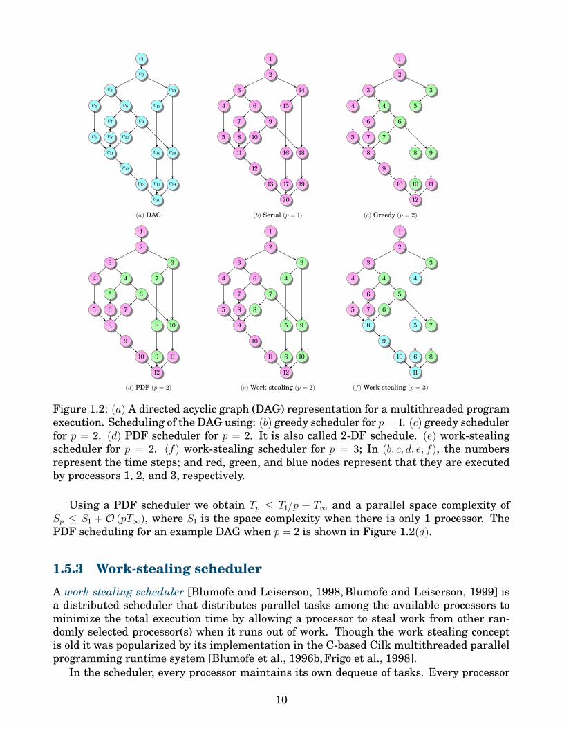
Figure 1.2: (a) A directed acyclic graph (DAG) representation for a multithreaded programexecution. Scheduling of the DAG using: (b) greedy scheduler for p = 1. (c) greedy schedulerfor p = 2. (d) PDF scheduler for p = 2. It is also called 2-DF schedule. (e) work-stealingscheduler for p = 2. (f) work-stealing scheduler for p = 3; In (b, c, d, e, f), the numbersrepresent the time steps; and red, green, and blue nodes represent that they are executedby processors 1, 2, and 3, respectively.

Using a PDF scheduler we obtain Tp ≤ T1/p + T∞ and a parallel space complexity ofSp ≤ S1 + O (pT∞), where S1 is the space complexity when there is only 1 processor. ThePDF scheduling for an example DAG when p = 2 is shown in Figure 1.2(d).

1.5.3 Work-stealing schedulerA work stealing scheduler [Blumofe and Leiserson, 1998, Blumofe and Leiserson, 1999] isa distributed scheduler that distributes parallel tasks among the available processors tominimize the total execution time by allowing a processor to steal work from other ran-domly selected processor(s) when it runs out of work. Though the work stealing conceptis old it was popularized by its implementation in the C-based Cilk multithreaded parallelprogramming runtime system [Blumofe et al., 1996b,Frigo et al., 1998].

In the scheduler, every processor maintains its own dequeue of tasks. Every processor

10

pops ready threads for execution and pushes spawned threads from its dequeue. Whenevera processors runs out of tasks, it steals from the top of the dequeue of a processor selectedat random.

For any parallel algorithm that is run under the randomized work-stealing scheduleron a parallel machine with private caches, the expected parallel running time [Arora et al.,2001] and the parallel cache complexity [Acar et al., 2000] is given by Tp = T1/p + O (T∞)and Qp = O (Q1 + p(M/B)T1), respectively. Also, the parallel space complexity is boundedas Sp ≤ pS1, where S1 is the serial space complexity. The work-stealing scheduling for anexample DAG when p = 2 and p = 3 are shown in Figures 1.2(e, f) respectively. Workstealing schedulers perform very well in practice and hence are used in Cilk [Blumofeet al., 1996b,Frigo et al., 1998], Cilk++ [Leiserson, 2010], Intel Cilk Plus [Plus, 2016], andOpenMP [Chapman et al., 2008]. They are also used in Java, Microsoft Visual Studio,GCC, and several other runtime systems.

1.5.4 Space-bound scheduler

A space-bounded scheduler [Chowdhury et al., 2013, Blelloch et al., 2011, Simhadri et al.,2014] was designed to overcome the limitation of the work-stealing scheduler and achieveoptimal parallel cache efficiency. The scheduler works for recursive divide-and-conquerparallel computation where a constant number of subtasks are generated by any task. Inthis scheduling method, the programmer sends a space bound (the upper bound on theamount of space that will be consumed by a task) of a task as a hint to the scheduler.When a task is anchored to a cache at some level, then the task will only be executed bythe processors under the subtree rooted at that cache.

For an algorithm that is run under the space-bounded scheduler, Tp = Θ (T1/p) andQp = O (Q1). The scheduler cannot be used to schedule the computation DAG of Figure 1.2(a) because the scheduler works only for trees of constant branch factor.

1.6 Algorithm design techniquesAlgorithm design techniques are like problem-solving strategies that give generic methodsand processes to crack algorithmic problems. There is an old proverb: “Give a man a fishand you feed him for a day; teach a man to fish and you feed him for a lifetime.” Adaptingthe proverb to algorithm design, we can state: “Give a man an algorithm and you solvehis current algorithmic problem; teach a man several algorithm design techniques and yousolve most of his algorithmic problems.”

There are several algorithm design strategies [Levitin, 2011] that can be used to de-sign new algorithms for new problems such as brute force, divide-and-conquer, decrease-and-conquer, transform-and-conquer, greedy technique, dynamic programming, iterativeimprovement, backtracking, and branch-and-bound.

The algorithms presented in this dissertation use a combination of the two algorithmdesign techniques: divide-and-conquer and dynamic programming. In subsequent sections,we will briefly describe the important aspects of the two algorithm design techniques.

11

1.6.1 Divide-and-conquerDivide-and-conquer is a powerful algorithm design strategy used to solve a problem bybreaking it down into smaller and simpler subproblems. The general plan of a divide-and-algorithm is as follows:

1. [Divide.] The given problem is divided into smaller subproblems (typically the sub-problems are independent and are of the same size).

2. [Conquer.] The subproblems are solved (typically using recursion)3. [Combine.] If necessary, the solutions to the subproblems are combined to form the

solution to the original problem.Recursive divide-and-conquer algorithms have the following advantages:

O [Complexity analysis.] They can be represented succinctly and can be analyzed forcomplexities using recurrence relations [Bentley, 1980].

O [Efficiency.] They are usually efficient [Levitin, 2011] in the sense that they reducethe total number of computations. E.g.: Comparison-based sorting algorithms thatuse divide-and-conquer require O (n log n) comparisons.

O [Easy parallelization.] They can be parallelized easily [Mou and Hudak, 1988, Blel-loch and Maggs, 2010] as the subproblems are typically independent, which can berun in parallel.

O [Cache-efficiency and cache-obliviousness.] They often are (or can be made) cache-efficient and cache-oblivious [Frigo et al., 1999, Chatterjee et al., 2002, Frens andWise, 1997].

O [Processor-obliviousness.] They often are (or can be made) processor-oblivious [Frigoet al., 1999,Chowdhury and Ramachandran, 2008].

O [Energy efficiency.] They can be energy efficient as they reduce the total number ofcomputations or the number of cache misses [Tithi et al., 2015].

For example, some of the fastest sorting algorithms such as merge sort and quicksortare based on divide-and-conquer.

1.6.2 Dynamic programming (DP)Dynamic programming (DP) is an algorithm design technique used to solve a problemby breaking it down into smaller and simpler subproblems. The method is used to solveproblems that have the properties of overlapping subproblems and optimal substructure.DP is especially used to solve optimization problems. Surprisingly, many combinatorialproblems that typically require an exponential time for the standard algorithms to solve,can be solved in polynomial time and space using DP. This is the reason some algorithmistscompare DP to a magical wand that turns stones into gold.

DP is used in a variety of fields such as operations research, parsing of ambiguouslanguages [Giegerich et al., 2004], sports and games [Romer, 2002, Duckworth and Lewis,1998,Smith, 2007], economics [Rust, 1996], finance [Robichek et al., 1971], and agriculture[Kennedy, 1981]. In computational biology, several significant problems such as protein-homology search, gene-structure prediction, motif search, analysis of repetitive genomicelements, RNA secondary-structure prediction, and interpretation of mass spectrometrydata [Bafna and Edwards, 2003,Durbin et al., 1998,Gusfield, 1997,Waterman et al., 1995]make use of dynamic programming.

In general, dynamic programming can be described as filling a table efficiently. The

12

table to be filled is called DP table and it consists of cells in a grid format. Initially, only afew cells are filled. Every cell can be computed using the values of already computed cellsusing a recurrence relation. Typically, all the cells of the DP table has to be filled using therecurrence relation. Often, we will be interested in the final values of one or more cells ofthe DP table, we call goal cells.

Dynamic programming can be implemented in two ways:O [Top-down.] In this approach (also called memoization), the cells that the goal cell(s)

depend upon are computed and stored. This process happens recursively (from root toleaves in the recursion tree) and only those cells that are required are stored / cached.The approach might lead to more space usage due to recursion.

O [Bottom-up.] In this approach, all cells will be computed exactly once in a bottom-up fashion (from leaves to root in the recursion tree) finally reaching the goal cell(s).This approach is the most widely used approach to implement dynamic programmingalgorithms.

Dynamic programming algorithms have the following advantages:O [Efficiency.] Several problems that require exponential time naively can be solved

using DP in polynomial time.O [Suited for discrete optimization problems.] DP is well-suited to solve discrete opti-

mization (minimization or maximization) problems as it explores all possible waysand selects the one that optimizes a given condition.

Methods to solve discrete optimization problems are called mathematical programming(or mathematical optimization) methods [Lew and Mauch, 2006]. It includes methods suchas linear programming, quadratic programming, iterative methods, dynamic programmingetc. There are efficient algorithms such as simplex method to solve linear programmingproblems. However, there is no universal efficient algorithm to solve all dynamic program-ming problems largely due of its generality.

Differences between plain recursion and dynamic programmingConsider the Fibonacci example. We know that the Fibonacci number F (i) is defined re-cursively as

F (i) =

i if i = 0 or 1,F (i− 1) + F (i− 2) if i > 1.

(1.1)

The recursion tree for this computation is given in Figure 1.3. The complexity of thisalgorithm (or the number of nodes in the recursion tree) is of the order Θ (φn), where φ isthe golden ratio. Using dynamic programming, we can write the recurrence as

F [i] =

i if i = 0 or 1,F [i− 1] + F [i− 2] if i > 1.

(1.2)

The recursion-DAG is shown in Figure 1.3. The complexity improves drastically to Θ (n).A summary table of the differences between simple recursion and dynamic programmingtechniques is given in Table 1.1.

In dynamic programming, finding the subproblems is the toughest part. In fact, de-pending on the identified subproblems, a problem can be solved in different ways using thesame dynamic programming technique.

13

F(5)

F(4)

F(3)

F(2)

F(1) F(0)

F(1)

F(2)

F(1) F(0)

F(3)

F(2)

F(1) F(0)

F(1)

F(5)

F(4)

F(3)

F(2)

F(1)F(0)

Figure 1.3: Computation of the Fibonacci number F(5) with base cases represented byrectangles. Left: Recursion tree when simple recursion is used. Right: Computation DAGwhen dynamic programming is used.

Feature Recursion Dynamic programmingExecution Top-down Bottom-upStoring / caching No YesUnrolling Recursion tree Computation DAGComplexity Exponential (typically) PolynomialSubproblems Overlapping / independent OverlappingRecurrence Uses parentheses (to denote functions) Uses square brackets (to denote table)

Table 1.1: Differences between recursion and dynamic programming.

1.6.3 Divide-and-conquer dynamic programmingWe can combine divide-and-conquer and dynamic programming techniques. The divide-and-conquer algorithms to solve dynamic programming problems are superior to existingalgorithms both in theory and in practice. Such algorithms have all the advantages ofdivide-and-conquer (with the exception of reducing the total number of computations). Of-ten, the algorithms are:

O [Efficient.] – cache-efficient, parallel, and energy efficient.O [Portable.] – cache-oblivious and processor-oblivious.O [Robust.] – cache-adaptive.Due to all the reasons mentioned above, divide-and-conquer technique is by far the

most powerful way to implement dynamic programming algorithms. Almost all of ouralgorithms presented in this dissertation are based on divide-and-conquer except the algo-rithms that discover them.

1.7 Dynamic programming implementationsDynamic programs are described through recurrence relations that specify how the cells ofa DP table must be filled using already computed values for other cells. Dynamic programsare traditional implemented iteratively i.e., using series of loops. Standard iterative algo-rithms do not have temporal locality, do not achieve very high parallelism (typically, forproblems having complicated non-local dependencies), and have poor bandwidth efficiency.

14

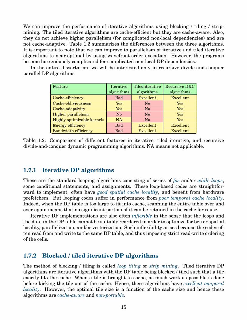
We can improve the performance of iterative algorithms using blocking / tiling / strip-mining. The tiled iterative algorithms are cache-efficient but they are cache-aware. Also,they do not achieve higher parallelism (for complicated non-local dependencies) and arenot cache-adaptive. Table 1.2 summarizes the differences between the three algorithms.It is important to note that we can improve to parallelism of iterative and tiled iterativealgorithms to near-optimal by using wavefront-order execution. However, the programsbecome horrendously complicated for complicated non-local DP dependencies.

In the entire dissertation, we will be interested only in recursive divide-and-conquerparallel DP algorithms.

Feature Iterative Tiled iterative Recursive D&Calgorithms algorithms algorithms

Cache-efficiency Bad Excellent ExcellentCache-obliviousness Yes No YesCache-adaptivity Yes No YesHigher parallelism No No YesHighly optimizable kernels NA No YesEnergy efficiency Bad Excellent ExcellentBandwidth efficiency Bad Excellent Excellent

Table 1.2: Comparison of different features in iterative, tiled iterative, and recursivedivide-and-conquer dynamic programming algorithms. NA means not applicable.

1.7.1 Iterative DP algorithmsThese are the standard looping algorithms consisting of series of for and/or while loops,some conditional statements, and assignments. These loop-based codes are straightfor-ward to implement, often have good spatial cache locality, and benefit from hardwareprefetchers. But looping codes suffer in performance from poor temporal cache locality.Indeed, when the DP table is too large to fit into cache, scanning the entire table over andover again means that no significant portion of it can be retained in the cache for reuse.

Iterative DP implementations are also often inflexible in the sense that the loops andthe data in the DP table cannot be suitably reordered in order to optimize for better spatiallocality, parallelization, and/or vectorization. Such inflexibility arises because the codes of-ten read from and write to the same DP table, and thus imposing strict read-write orderingof the cells.

1.7.2 Blocked / tiled iterative DP algorithmsThe method of blocking / tiling is called loop tiling or strip mining. Tiled iterative DPalgorithms are iterative algorithms with the DP table being blocked / tiled such that a tileexactly fits the cache. When a tile is brought to cache, as much work as possible is donebefore kicking the tile out of the cache. Hence, these algorithms have excellent temporallocality. However, the optimal tile size is a function of the cache size and hence thesealgorithms are cache-aware and non-portable.

15

1.7.3 Recursive divide-and-conquer DP algorithmsOur two most important priorities are: performance and portability. Iterative algorithmssuffer in performance and tiled iterative algorithms are non-portable. These limitationsare handled by the recursive divide-and-conquer algorithms as they lead to both high per-formance and portability.

A necessary condition for an algorithm for a problem to have temporal locality is thatthe work (total number of computations) done by the algorithm must be asymptoticallylarger than the total space usage.

Hence, if we have a cache-oblivious recursive divide-and-conquer DP algorithm for aproblem, it does not necessarily mean that it is cache-efficient (through temporal locality).The minimum criteria the algorithm has to satisfy is that the average number of computa-tions per unit of space must be ω (1) (asymptotically more than constant).

Recursive divide-and-conquer algorithms consist of one or more recursive functions.Because of their recursive nature such algorithms are known to have excellent (and oftenoptimal) temporal locality. Efficient implementations of these algorithms use iterative ker-nels when the problem size becomes reasonably small. But unlike standard loop-based DPcodes, the loops inside these iterative kernels can often be easily reordered, thus allowingfor better spatial locality, vectorization, parallelization, and other optimizations.

The sizes of the iterative kernels are determined based on vectorization efficiency andoverhead of recursion, and not on cache sizes, and thus the algorithms remain cache-oblivious and portable. Unlike tiled looping codes these algorithms are also cache-adaptive[Bender et al., 2014] — they passively self-adapt to fluctuations in available cache spacewhen caches are shared with other concurrently running programs.

1.8 Automatic algorithm discoveryAutomation is a revolutionary idea. Automation is the process of using automatic devicesand computing machines to replace the routine human effort and labor. For example,online shopping systems such as amazon.com, mass manufacturing of products, ATM ma-chines, ticket machines, food machines, automated testing, robotics, GPS navigation, vehi-cles, traffic lights, video surveillance, automated replies, self-driving cars, and thousandsof other stuff. Automation has several advantages:

O [Saves time.] Automation replaces manual effort with machine effort. Hence, it savesa lot of time, energy, and money of humans. Reducing the time improves productivity.

O [Increases accuracy.] Machines perform the work they are designed or programmedto do. As they do not take decisions (like we do), they follow a human’s command asit is and they do not deviate from what is supposed to be done. Hence, this machineprocess maintains the accuracy and does not give an opportunity for humans to makemistakes :).

O [Deeper understanding of the process.] Automating a human effort leads to a deeperunderstanding of the process itself and this understanding might be very useful.

In computer science, automation is majorly used to replace the human labor in the soft-ware development process. Automation is also used to some extent in problem solving.There are automated frameworks for domain specific languages (DSL), e.g.: Pochoir [Tanget al., 2011], automatically generate high performing implementations for certain problems

16

from known efficient algorithms. However, there is little work for automation of nontrivialdesign of algorithms [Kant, 1985] given just the problem specifications. This dissertationis the first major step in the science of discovery of nontrivial efficient cache-oblivious al-gorithms.

Designing algorithms is hard. Discovering a fast and portable algorithm requires exper-tise from different fields such as algorithmics, data structures, parallel algorithms, com-puter architecture, compiler design, operating system, and so on. A domain expert (human)who has a deeper understanding of the problem and who has a good experience in solvingsimilar problems can design an efficient algorithm given sufficient time, energy, and re-sources. However, this method does not scale very well when the number of problems tobe solved gets bigger and bigger. Also, the designed algorithms must be proved correct,analyzed for their complexities, and implemented. Hence, an intelligent way to addressthis issue is to build machines to solve problems automatically or in computer science ter-minology – design an algorithm that discovers other algorithms.

Having a system that can automatically generate highly efficient parallel implemen-tations from easy-to-write and concise specifications of the problem is extremely useful.Computational scientists who specialize in subjects other than computer science such asbiology, chemistry, physics, material science, and so on without a formal training in com-puter science find it difficult to develop highly efficient algorithms for the state-of-the-artsupercomputers. A system that automates the complicated task of efficient algorithm dis-covery saves hundreds of thinking hours and brings the power of supercomputing closer toprogrammers without deep computer science (CS) background.

1.8.1 Program synthesisProgram synthesis [Steier and Anderson, 2012] is a field in computer science that is re-lated to automatic programming or automatic algorithm design. The idea for programsynthesis originated in the 1960s with the aim to automate programming using artificialintelligence. In recent decades, formal mathematical methods are used to specify, derive(using deductive methods), and verify (using formal verification methods such as theoremprovers) algorithms.

There is a large literature using formal methods to synthesize programs [Klonatos et al.,2013, Armando et al., 1999]. However, all these methods use different types of logicalcalculus and they require a lot of user interaction such as specifying the functions or otherparameters that the algorithm to be designed must use. This is the reason most of thesemethods are not fully automatic.

1.8.2 Polyhedral compilersThere are several systems to automatically parallelize programs [Bondhugula et al., 2008,Banerjee et al., 1993, Bae et al., 2013, Feautrier, 1996, Hendren and Nicolau, 1990, Cam-panoni et al., 2012]. Some systems are described for loops and other systems are describedfor trees and DAGs. The literature of parallelizers is vast. A majority of these parallelizersuse loop transformations in the polyhedral model [Feautrier and Lengauer, 2011]. Some ofthese systems can also optimize the programs for cache locality and hence they generatecache-efficient parallel algorithms.

17

A few drawbacks of the polyhedral compilers or parallelizers are:O [Cache-awareness.] The generated algorithms depend on the cache parameters and

hence are cache-aware and not cache-oblivious.O [Loop programs on arrays.] The application of the model is limited to loops that work

on arrays.In the polyhedron model, the point-sets form a polyhedra in Zd. The point-sets are

represented as solutions to a system of affine inequalities Ax ≤ b, where A is a constantmatrix, x is a variable vector, and b is a constant vector. The solutions can be found usingloop transformations and integer linear programming.

1.9 Dissertation outlineIn this section, we give the statement of the dissertation; contributions of the dissertationto theoretical and practical computer science; and finally the organization of topics in thedissertation.

1.9.1 Dissertation statementThe main motivation for the work in the dissertation is to bring automated algorithm de-sign to the masses. Developing algorithms(s) (resp. framework(s)) that can be used toautomatically (resp. semi-automatically) discover algorithms can be very useful to compu-tational scientists and programmers with less expertise in computer science. This disser-tation gives evidence to support the statement:

It is possible to develop algorithm(s) / framework(s) to automatically / semi-automatically discover algorithms that are simultaneously nontrivial, fast,portable, and robust, which can be used to solve to a wide class of dynamic pro-gramming problems.

1.9.2 Dissertation contributionsThe major contributions of the dissertation are as follows:

O [Autogen.] We design an algorithm called Autogen that for a wide class of dynamicprogramming problems automatically discovers nontrivial efficient (cache-efficient,parallel, and energy-efficient), portable (processor- and cache-oblivious), and robust(processor- and cache-adaptive) recursive divide-and-conquer algorithms given itera-tive descriptions of the DP recurrences. We prove the correctness of Autogen, analyzethe cache-complexities of Autogen-discovered algorithms, and implement Autogen.

O [Autogen-Wave.] We design a framework called Autogen-Wave that for a wide classof dynamic programming problems semi-automatically discovers non-trivial recur-sive divide-and-conquer wavefront algorithms from standard divide-and-conquer al-gorithms and DP recurrences. Autogen-Wave is the sequel of Autogen as it takes theAutogen-discovered algorithms as input and discovers algorithms that have near-optimal parallelism (retaining all the other advantages of the input algorithms).

18

Autogen algorithm

D&C DP algorithms

D&C DP wavefrontalgorithms

Autogen-Wave

(Chapter 2)

(Appendix A)

(Chapter 3)

(Appendix B)

D&C DP hybridalgorithms(Appendix E)

automaticallydiscover

improve parallelismwithout extra space

recursionnot allowed

semi-automaticallydiscover

problems withirregular dependencies

framework

Autogen-Tradeoff

(Chapter 6)


framework

improve parallelismwith extra space

Viterbi algorithm(Chapter 4)

D&C DP tiledalgorithms

Autogen-Fractile

(Chapter 5)

(Appendix D)


framework

Other algorithms(Appendix C)

Figure 1.4: Dissertation map.

O [Viterbi.] Autogen cannot be directly used to develop efficient algorithms for data-dependent / data-sensitive dynamic programs. The Viterbi recurrence is an extremelyimportant example of a data-dependent dynamic program for which there is no ef-ficient resource-oblivious algorithm. We design the first provably correct efficientresource-oblivious parallel Viterbi algorithm.

O [Autogen-Fractile.] We design a framework called Autogen-Fractile that can be usedto semi-automatically discover efficient cache-aware tiled algorithms based on recur-sive divide-and-conquer, for a wide class of dynamic programming problems. We provestrong theoretical bounds on cache locality and parallelism. We design the fastestGPU algorithms for several dynamic programs using the framework.

O [Autogen-Tradeoff.] We design a framework called Autogen-Tradeoff that can beused to design algorithms to asymptotically increase the parallelism of some of theAutogen-discovered algorithms without affecting cache-efficiency, but using extra space.

The relation between all the chapters in the dissertation and how they relate to thetheme of the dissertation is shown in Figure 1.4. A list of my papers appear in Table1.3. The work in the dissertation is a joint contribution. The experiments (included inthe dissertation for completeness) are the work of Jesmin Jahan Tithi, Stephen Tschudi,Rathish Das, Mohammad Mahdi Javanmard, Yunpeng Xiao, and Isha Khanna.

19

No. Paper Conf / journal In thesis?Major contribution1 Autogen: Automatic Discovery of Cache-Oblivious Parallel Recursive Algorithms

for Solving Dynamic ProgramsPPoPP 2016 Chap. 2

with Rezaul Chowdhury, Jesmin Jahan Tithi, Charles Bachmeier, Bradley Kusz-maul, Charles E. Leiserson, Armando Solar-Lezama, & Yuan Tang

(Invited to TOPC)

2 Autogen: Automatic Discovery of Cache-Oblivious Parallel Recursive Algorithmsfor Solving Dynamic Programs

Under prep. Chap. 2

with Rezaul Chowdhury, Jesmin Jahan Tithi, Charles Bachmeier, Bradley Kusz-maul, Charles E. Leiserson, Armando Solar-Lezama, & Yuan Tang

3 Provably Efficient Scheduling of Cache-Oblivious Wavefront Algorithms Under prep. Chap. 3with Rezaul Chowdhury, Jesmin Jahan Tithi, & Yuan Tang

4 An Efficient Cache-Oblivious Parallel Viterbi Algorithm Euro-Par 2016 Chap. 4with Rezaul Chowdhury, Vivek Pradhan, Jesmin Jahan Tithi, & Yunpeng Xiao

5 A Framework for Designing External-Memory RAM-Oblivious GPU Algorithms forDynamic Programs

Under review Chap. 5

with Rezaul Chowdhury, Rathish Das, Mohammad Mahdi Javanmard, & StephenTschudi

6 Space-Parallelism Tradeoff for Cache-Oblivious Parallel Algorithms Under prep. Chap. 6with Rezaul Chowdhury, Mohammad Mahdi Javanmard, Isha Khanna, Pre-madurga Kolli, & Stephen Tschudi

7 Divide-and-Conquer Variants of Bubble, Selection, & Insertion Sorts Under prep. Chap. Awith Rezaul Chowdhury

8 A Framework to Discover Combinatorial Algorithms Under prep. 7

with Rama Badrinath & Abhiram Natarajan9 Premtuatoins & PAttERns Under prep. 7

with Rezaul Chowdhury10 The Range 1 Query (R1Q) Problem COCOON 2014 7

with Michael A. Bender, Rezaul Chowdhury, Samuel McCauley, & Yuan Tang (Invited to TCS)11 The Range 1 Query (R1Q) Problem TCS 2016 7

with Michael A. Bender, Rezaul Chowdhury, Samuel McCauley, & Yuan TangMinor contribution12 Cache-Oblivious Wavefront: Improving Parallelism of Recursive Dynamic Pro-

gramming Algorithms Without Losing Cache-EfficiencyPPoPP 2015 7

with Yuan Tang, Ronghui You, Haibin Kan, Jesmin Jahan Tithi, & Rezaul Chowd-hury

13 The I/O Complexity of Computing Prime Tables LATIN 2016 Chap. Awith Michael A. Bender, Rezaul Chowdhury, Alex Conway, Martin Farach-Colton,Rob Johnson, Samuel McCauley, Bertrand Simon, & Shikha Singh

(part)

14 High-Performance Energy-Efficient Recursive Dynamic Programming withMatrix-Multiplication-like Flexible Kernels

IPDPS 2015 Chap. A

with Jesmin Jahan Tithi, Aakrati Talati, Sonal Aggarwal, & Rezaul Chowdhury (part)

Table 1.3: My papers. In mathematics and theoretical computer science, we often followthe convention of listing authors in alphabetical order of last names.

1.9.3 Dissertation organizationThe organization of the topics in the dissertation is as follows. We present our Autogenalgorithm, its proof of correctness, and cache complexity of Autogen-discovered algorithmsin Chapter 2. We present recursive divide-and-conquer algorithms to several dynamicprogramming problems in Appendix A. In Chapter 3, we present our Autogen-Wave frame-work that can be used to discover divide-and-conquer wavefront algorithms. We presentthe Autogen-Wave-discovered divide-and-conquer wavefront algorithms in Appendix B. InChapter 4, we present a provably cache-efficient cache-oblivious parallel Viterbi algorithm.Efficient algorithms are presented for DP problems with irregular data dependencies inAppendix C. In Chapter 5, we present the Autogen-Fractile framework that can be used

20

to discover highly efficient recursive divide-and-conquer-based tiled algorithms. In Ap-pendix D, we present several divide-and-conquer tiled algorithms. Finally, we present ourAutogen-Tradeoff framework in Chapter 6 and present hybrid algorithms in Appendix E.

21

Chapter 2

Automatic Discovery of EfficientDivide-&-Conquer DP Algorithms

We present Autogen — an algorithm that for a wide class of dynamic programming (DP)problems automatically discovers highly efficient cache-oblivious parallel recursive divide-and-conquer algorithms from inefficient iterative descriptions of DP recurrences. Autogenanalyzes the set of DP table locations accessed by the iterative algorithm when run on aDP table of small size, and automatically identifies a recursive access pattern and a cor-responding provably correct recursive algorithm for solving the DP recurrence. We useAutogen to autodiscover efficient algorithms for several well-known problems. Our ex-perimental results show that several autodiscovered algorithms significantly outperformparallel looping and tiled loop-based algorithms. Also these algorithms are less sensitiveto fluctuations of memory and bandwidth compared with their looping counterparts, andtheir running times and energy profiles remain relatively more stable. To the best of ourknowledge, Autogen is the first algorithm that can automatically discover new nontrivialdivide-and-conquer algorithms.

2.1 IntroductionAutogen is an algorithm for automatic discovery of efficient recursive divide-and-conquerdynamic programming (DP) algorithms for multicore machines from naive iterative de-scriptions of the dynamic programs. DP [Bellman, 1957, Sniedovich, 2010, Cormen et al.,2009] is a widely used algorithm design technique that finds optimal solutions to a problemby combining optimal solutions to its overlapping subproblems, and explores an otherwiseexponential sized search space in polynomial time by saving solutions to subproblems in atable and never recomputing them. DP is extensively used in computational biology [Bafnaand Edwards, 2003,Durbin et al., 1998,Gusfield, 1997,Waterman et al., 1995], and in manyother application areas including operations research, compilers [Lew and Mauch, 2006],sports [Romer, 2002, Duckworth and Lewis, 1998], games [Smith, 2007], economics [Rust,1996], finance [Robichek et al., 1971] and agriculture [Kennedy, 1981].

Dynamic programs are described through recurrence relations that specify how the cellsof a DP table must be filled using already computed values for other cells. Such recurrencesare commonly implemented using simple algorithms that fill out DP tables iteratively.These loop-based codes are straightforward to implement, often have good spatial cache

22

locality1, and benefit from hardware prefetchers. But looping codes suffer in performancefrom poor temporal cache locality2. Iterative DP implementations are also often inflexiblein the sense that the loops and the data in the DP table cannot be suitably reorderedin order to optimize for better spatial locality, parallelization, and/or vectorization. Suchinflexibility arises because the codes often read from and write to the same DP table, andthus imposing strict read-write ordering of the cells.

Recursive divide-and-conquer DP algorithms (see Table 2.1) can often overcome manylimitations of their iterative counterparts. Because of their recursive nature such algo-rithms are known to have excellent (and often optimal) temporal locality. Efficient im-plementations of these algorithms use iterative kernels when the problem size becomesreasonably small. But unlike in standard loop-based DP codes, the loops inside theseiterative kernels can often be easily reordered, thus allowing for better spatial locality,vectorization, parallelization, and other optimizations. The sizes of the iterative kernelsare determined based on vectorization efficiency and overhead of recursion, and not oncache sizes, and thus the algorithms remain cache-oblivious3 [Frigo et al., 1999] and moreportable than cache-aware tiled iterative codes. Unlike tiled looping codes these algorithmsare also cache-adaptive [Bender et al., 2014] — they passively self-adapt to fluctuations inavailable cache space when caches are shared with other concurrently running programs.

For example, consider the dynamic program for solving the parenthesis problem [Galiland Park, 1994] in which we are given a sequence of characters S = s1 · · · sn and we arerequired to compute the minimum cost of parenthesizing S. Let C[i, j] denote the minimumcost of parenthesizing si · · · sj. Then the DP table C[0 : n, 0 : n] is filled up using thefollowing recurrence:

C[i, j] =

∞ if 0 ≤ i = j ≤ n,vj if 0 ≤ i = j − 1 < n,mini≤k≤j

(C[i, k] + C[k, j]) + w(i, k, j) if 0 ≤ i < j − 1 < n;(2.1)

where the vj ’s and function w(·, ·, ·) are given.Figure 3.1 shows a serial looping code LOOP-PARENTHESIS implementing Recurrence

3.1. Though the code is really easy to understand and write, it suffers from poor cacheperformance. Observe that the innermost loop scans one row and one column of the sameDP table C. Assuming that C is of size n × n and C is too large to fit into the cache, eachiteration of the innermost loop may incur one or more cache misses leading to a total ofΘ (n3) cache misses in the ideal-cache model [Frigo et al., 1999]. Such extreme inefficiencyin cache usage makes the code bandwidth-bound. Also this code does not have any paral-lelism as none of the three loops can be parallelized. The loops cannot also be reorderedwithout making the code incorrect4 which makes the code difficult to optimize.

Figure 3.1 shows the type of parallel looping code PAR-LOOP-PARENTHESIS one wouldwrite to solve Recurrence 3.1. We can analyze its parallel performance under the work-span model [Cormen et al., 2009] (chapter 27) which defines the parallelism of a code

1Spatial locality — whenever a cache block is brought into the cache, it contains as much useful data aspossible.

2Temporal locality — whenever a cache block is brought into the cache, as much useful work as possibleis performed on this data before removing the block from the cache.

3Cache-oblivious algorithms — algorithms that do not use the knowledge of cache parameters in thealgorithm description.

4compare this with iterative matrix multiplication in which all 6 permutations of the three nested loopsproduce correct results

23

PAR-LOOP-PARENTHESIS(C, n)

1. for t← 2 to n− 1 do2. parallel for i← 1 to n− t do3. j ← t+ i4. for k ← i+ 1 to j do5. C[i, j]← min

(C[i, j], C[i, k]+C[k, j] + w(i, k, j)

)

Parallelizer

LOOP-PARENTHESIS(C, n)

1. for i← n− 1 to 0 do2. for j ← i+ 2 to n do3. for k ← i to j do4. C[i, j]← min

(C[i, j], C[i, k]+C[k, j] + w(i, k, j)

)

Autogen

Apar(〈X,X,X〉)

1. if X is a small matrix then Aloop-par(〈X,X,X〉)2. else3. par: Apar(〈X11, X11, X11〉), Apar(〈X22, X22, X22〉)4. Bpar(〈X12, X11, X22〉)

Bpar(〈X,U, V 〉)

1. if X is a small matrix then Bloop-par(〈X,U, V 〉)2. else3. Bpar(〈X21, U22, V11〉)4. par: Cpar(〈X11, U12, X21〉), Cpar(〈X22, X21, V12〉)5. par: Bpar(〈X11, U11, V11〉), Bpar(〈X22, U22, V22〉)6. Cpar(〈X12, U12, X22〉)7. Cpar(〈X12, X11, V12〉)8. Bpar(〈X12, U11, V22〉)

Cpar(〈X,U, V 〉)

1. if X is a small matrix then Cloop-par(〈X,U, V 〉)2. else3. par: Cpar(〈X11, U11, V11〉), Cpar(〈X12, U11, V12〉),

Cpar(〈X21, U21, V11〉), Cpar(〈X22, U21, V12〉)4. par: Cpar(〈X11, U12, V21〉), Cpar(〈X12, U12, V22〉),

Cpar(〈X21, U22, V21〉), Cpar(〈X22, U22, V22〉)

Figure 2.1: Left upper half: A parallel looping code that evaluates Recurrence 3.1. Leftlower half: Autogen takes the serial parenthesis algorithm as input and automaticallydiscovers a recursive divide-and-conquer cache-oblivious parallel algorithm. Initial call tothe divide-and-conquer algorithm is Apar(〈C,C,C〉), where C is an n × n DP table and n isa power of 2. The iterative base-case kernel of a function Fpar is Floop-par. Right: Pictorialrepresentation of the recursive divide-and-conquer algorithm discovered by Autogen. Datain the dark red blocks are updated using data from light blue blocks.

as T1/T∞, where Tp (p ∈ [1,∞)) is the running time of the code on p processing cores(without scheduling overhead). Clearly, the parallelism of PAR-LOOP-PARENTHESIS isΘ (n3) /Θ (n2) = Θ (n). If the size M of the cache is known the code can be tiled to improveits cache performance to Θ

(n3/

(B√M))

, where B is the cache line size. However, such

24

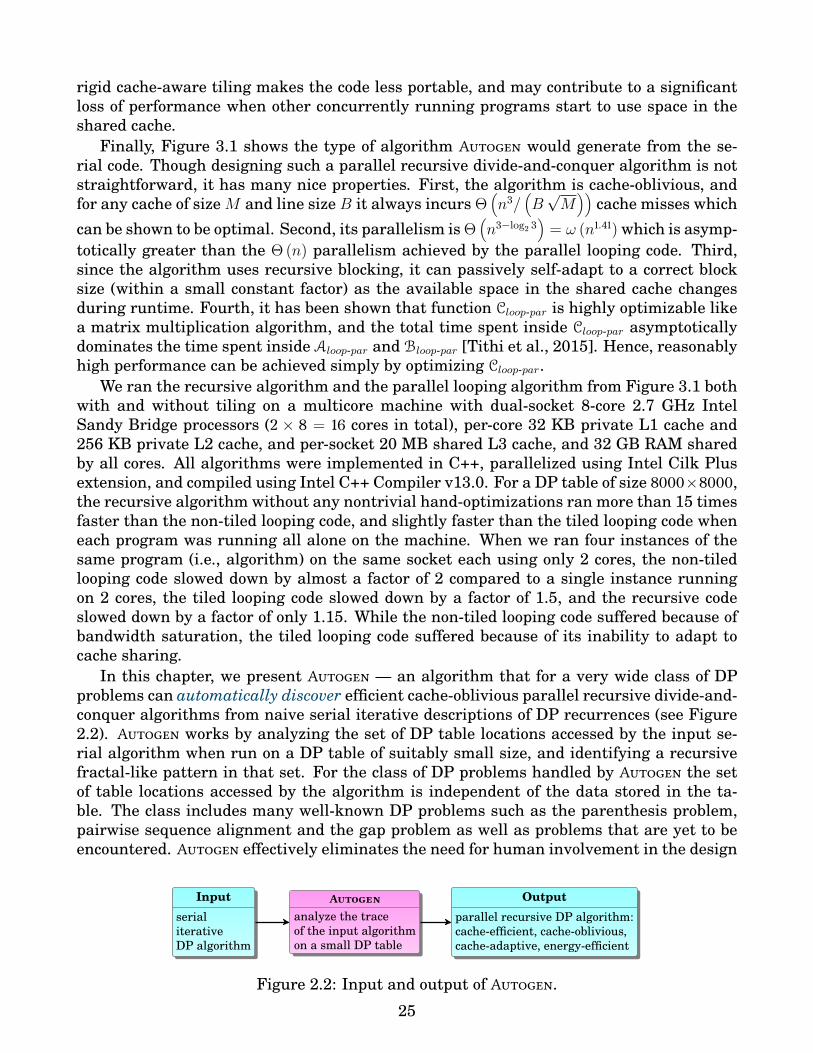
rigid cache-aware tiling makes the code less portable, and may contribute to a significantloss of performance when other concurrently running programs start to use space in theshared cache.

Finally, Figure 3.1 shows the type of algorithm Autogen would generate from the se-rial code. Though designing such a parallel recursive divide-and-conquer algorithm is notstraightforward, it has many nice properties. First, the algorithm is cache-oblivious, andfor any cache of size M and line size B it always incurs Θ

(n3/

(B√M))

cache misses whichcan be shown to be optimal. Second, its parallelism is Θ

(n3−log2 3

)= ω (n1.41) which is asymp-

totically greater than the Θ (n) parallelism achieved by the parallel looping code. Third,since the algorithm uses recursive blocking, it can passively self-adapt to a correct blocksize (within a small constant factor) as the available space in the shared cache changesduring runtime. Fourth, it has been shown that function Cloop-par is highly optimizable likea matrix multiplication algorithm, and the total time spent inside Cloop-par asymptoticallydominates the time spent inside Aloop-par and Bloop-par [Tithi et al., 2015]. Hence, reasonablyhigh performance can be achieved simply by optimizing Cloop-par.

We ran the recursive algorithm and the parallel looping algorithm from Figure 3.1 bothwith and without tiling on a multicore machine with dual-socket 8-core 2.7 GHz IntelSandy Bridge processors (2 × 8 = 16 cores in total), per-core 32 KB private L1 cache and256 KB private L2 cache, and per-socket 20 MB shared L3 cache, and 32 GB RAM sharedby all cores. All algorithms were implemented in C++, parallelized using Intel Cilk Plusextension, and compiled using Intel C++ Compiler v13.0. For a DP table of size 8000×8000,the recursive algorithm without any nontrivial hand-optimizations ran more than 15 timesfaster than the non-tiled looping code, and slightly faster than the tiled looping code wheneach program was running all alone on the machine. When we ran four instances of thesame program (i.e., algorithm) on the same socket each using only 2 cores, the non-tiledlooping code slowed down by almost a factor of 2 compared to a single instance runningon 2 cores, the tiled looping code slowed down by a factor of 1.5, and the recursive codeslowed down by a factor of only 1.15. While the non-tiled looping code suffered because ofbandwidth saturation, the tiled looping code suffered because of its inability to adapt tocache sharing.

In this chapter, we present Autogen — an algorithm that for a very wide class of DPproblems can automatically discover efficient cache-oblivious parallel recursive divide-and-conquer algorithms from naive serial iterative descriptions of DP recurrences (see Figure2.2). Autogen works by analyzing the set of DP table locations accessed by the input se-rial algorithm when run on a DP table of suitably small size, and identifying a recursivefractal-like pattern in that set. For the class of DP problems handled by Autogen the setof table locations accessed by the algorithm is independent of the data stored in the ta-ble. The class includes many well-known DP problems such as the parenthesis problem,pairwise sequence alignment and the gap problem as well as problems that are yet to beencountered. Autogen effectively eliminates the need for human involvement in the design

Autogen

analyze the traceof the input algorithmon a small DP table

InputserialiterativeDP algorithm

Outputparallel recursive DP algorithm:cache-efficient, cache-oblivious,cache-adaptive, energy-efficient

Figure 2.2: Input and output of Autogen.

25

I-DP R-DP

Work Serial cache Span Serial cache SpanProblem (T1) comp. (Q1) (T∞) comp. (Q1) (T∞)Parenthesis problem Θ (n3) Θ (n3) Θ (n2) Θ

(n3/(B

√M)

)Θ(nlog 3

)Floyd-Warshall’s APSP 3-D Θ (n3) Θ (n3/B) Θ (n log n) Θ (n3/B) O

(n log2 n

)Floyd-Warshall’s APSP 2-D Θ (n3) Θ (n3/B) Θ (n log n) Θ

(n3/(B

√M)

)Θ(n log2 n

)LCS / Edit distance Θ (n2) Θ (n2/B) Θ (n) Θ (n2/(BM)) Θ

(nlog 3

)Multi-instance Viterbi Θ (n3t) Θ (n3t/B) Θ (nt) Θ

(n3t/(B

√M)

)Θ (nt)

Gap problem Θ (n3) Θ (n3) Θ (n2) Θ(n3/(B

√M)

)Θ(nlog 3

)Protein accordion folding Θ (n3) Θ (n3/B) Θ (n2) Θ

(n3/(B

√M)

)Θ (n log n)

Spoken-word recognition Θ (n2) Θ (n2/B) Θ (n) Θ (n2/(BM)) Θ(nlog 3

)Function approximation Θ (n3) Θ (n3/B) Θ (n2) Θ

(n3/(B

√M)

)Θ(nlog 3

)Binomial coefficient O (n2) O (n2/B) Θ (n) Θ (n2/(BM)) Θ

(nlog 3

)Bitonic traveling salesman Θ (n2) Θ (n2/B) Θ (n) Θ (n2/(BM)) Θ (n log n)Matrix multiplication Θ (n3) Θ (n3/B) Θ (n) Θ

(n3/(B

√M)

)Θ (n)

Bubble sort Θ (n2) Θ (n2/B) Θ (n2) Θ (n2/(BM)) Θ (n)Selection sort Θ (n2) Θ (n2/B) Θ (n2) Θ (n2/(BM)) Θ (n)Insertion sort O (n2) O (n2/B) O (n2) O

(nlog 3/(BM log 3−1)

)O (n)

Table 2.1: Work (T1), serial cache complexity (Q1), and span (T∞) of I-DP and R-DP algo-rithms for several DP problems. Here, n = problem size, M = cache size, B = block size,and p = #cores. By Tp we denote running time on p processing cores. We assume that theDP table is too large to fit into the cache, and M = Ω

(Bd)

when Θ(nd)

is the size of the DPtable. On p cores, the running time is Tp = O (T1/p+ T∞) and the parallel cache complexityis Qp = O (Q1 + p(M/B)T∞) with high probability when run under the randomized work-stealing scheduler on a parallel machine with private caches. The problems in the lowersection are non-DP problems. For insertion sort, T1 for R-DP is O

(nlog 3

).

of efficient cache-oblivious parallel algorithms for all present and future problems in thatclass.

Our contributions. Our major contributions are as follows:(1) [Algorithmic.] We present Autogen — an algorithm that for a wide class of DP

problems automatically discovers highly efficient cache-oblivious parallel recursivedivide-and-conquer algorithms from iterative descriptions of DP recurrences. Auto-gen works by analyzing the DP table accesses (assumed to be independent of the datain the table) of an iterative algorithm on a table of small size, finding the dependen-cies among different orthants of the DP table recursively, and constructing a tree anddirected acyclic graphs that represent a set of recursive functions corresponding toa parallel recursive divide-and-conquer algorithm. We prove the correctness of thealgorithms generated by Autogen.

(2) [Experimental.] We have implemented a prototype of Autogen which we have usedto autogenerate efficient cache-oblivious parallel recursive divide-and-conquer algo-rithms (pseudocodes) from naive serial iterative descriptions of several DP recur-rences. We present experimental results showing that several autogenerated algo-rithms without any nontrivial hand-tuning significantly outperform parallel looping

26

codes in practice, and have more stable running times and energy profiles in a multi-programming environment compared to looping and tiling algorithms.

Related work. Systems for auto-generating fast iterative DP implementations (not algo-rithms) exist. The Bellman’s GAP compiler [Giegerich and Sauthoff, 2011] converts declar-ative programs into optimized C++ code. A semi-automatic synthesizer [Pu et al., 2011]exists which uses contraint-solving to solve linear-time DP problems such as maximal sub-string matching, assembly-line optimization and the extended Euclid algorithm.

There are systems to automatically parallelize DP loops. EasyPDP [Tang et al., 2012]requires the user to select a directed acyclic graph (DAG) pattern for a DP problem fromits DAG patterns library. New DAG patterns can be added to the library. EasyHPS [Duet al., 2013] uses the master-slave paradigm in which the master scheduler distributescomputable sub-tasks among its slaves, which in turn distribute subsubtasks among slavethreads. A pattern-based system exists [Liu and Schmidt, 2004] that uses generic program-ming techniques such as class templates to solve problems in bioinformatics. Parallelizingplugins [Reitzig, 2012] use diagonal frontier and row splitting to parallelize DP loops.

To the best of our knowledge, there has been no previous attempt to automate theprocess of discovering efficient cache-oblivious and cache-adaptive parallel recursive al-gorithms by analyzing the memory access patterns of naive serial iterative algorithms.The work that is most related to Autogen, but completely different in many aspects isPochoir [Tang et al., 2011]. Pochoir translates simple specifications of a stencil5 into high-performing parallel code implementing an efficient cache-oblivious parallel algorithm. WhilePochoir tailors the implementation of the same cache-oblivious algorithm (known as thetrapezoidal decomposition algorithm) to different stencil computations, Autogen discoversa (possibly) brand new efficient parallel cache-oblivious algorithm for every new DP prob-lem it encounters.

Compiler technology for automatically converting iterative versions of matrix programsto serial recursive versions is described in [Ahmed and Pingali, 2000]. The approach re-lies on heavy machineries such as dependence analysis (based on integer programming)and polyhedral techniques. Autogen, on the other hand, is a much simpler stand-alonealgorithm that analyzes the data access pattern of a given naive (e.g., looping) serial DPcode when run on a small example, and inductively generates a provably correct parallelrecursive algorithm for solving the same DP.

2.2 The Autogen algorithmIn this section, we present an algorithm called Autogen that automatically converts aniterative algorithm to an efficient cache-oblivious parallel recursive divide-and-conquer al-gorithm for a wide variety of DP problems.

Definition 1 (I-DP / R-DP / Autogen). Let P be a given DP problem specified througha DP recurrence. An iterative (or loop-based) algorithm for P is called I-DP. A cache-oblivious parallel recursive divide-and-conquer algorithm (if it exists) for P is called R-DP.The algorithm that automatically generates an R-DP given any implementation for P iscalled Autogen.

5a stencil is a dynamic program in which the value of a spatial cell at any time step depends on itsneighboring cells in a constant number of previous time steps

27

The input to Autogen can be any implementation (I-DP, tiled I-DP, R-DP, or someother implementation) of the given DP recurrence. As the simplest implementation of aDP recurrence is an iterative algorithm or I-DP, in this chapter we assume I-DPs as in-puts to Autogen.

AutogenI-DP R-DP

Algorithm. The four main steps of Autogen are:(1) [Cell-set generation.] A cell-set is generated from a sample run of the given I-DP on

a problem of small size. See Section 2.2.1.(2) [Algorithm-tree construction.] An algorithm-tree is constructed from the cell-set in

which each node represents a subset of the cell-set and follows certain rules. SeeSection 2.2.2.

(3) [Algorithm-tree labeling.] The nodes of the tree are labeled with function names andthese labels represent a set of recursive divide-and-conquer functions in an R-DP

under Assumption 1. See Section 2.2.3.(4) [Algorithm-DAG Construction.] For every unique function, we construct a directed

acyclic graph (DAG) that shows both the order in which the functions are to be exe-cuted and the parallelism involved. See Section 2.2.4.

We make the following assumption for an R-DP.

Assumption 1 (Number of functions). The number of distinct recursive functions in anR-DP is upper bounded by a constant.

Example. Autogen works for arbitrary d-D (d ≥ 1) DP problems under the assumption thateach dimension of the DP table is of the same length and is a power of 2. For simplicityof exposition, we explain Autogen by applying it on an I-DP for the parenthesis problem,which updates a 2-D DP table.

In the parenthesis problem [Galil and Park, 1994], we are given a sequence of charac-ters S = s1 · · · sn and we would like to compute the minimum cost of parenthesizing S. Thisproblem represents a class of problems such as optimal matrix chain multiplication, stringparsing for context-free grammar (e.g., CYK algorithm), RNA secondary structure pre-diction, optimal natural join of database tables (e.g., Selinger algorithm), construction ofoptimal binary search trees, optimal polygon triangulation, maximum perimeter inscribedpolygon, and offline job scheduling minimizing total flow time of jobs. Let C[i, j] denote theminimum cost of parenthesizing si · · · sj. Then, the DP table C[0 : n, 0 : n] is filled up usingthe following recurrence.

C[i, j] =


(C[i, k] + C[k, j]) + w(i, k, j) if 0 ≤ i < j − 1 < n;(2.2)

where vj ’s are given, and function w() can be computed without additional memory ac-cesses.

Based on the recurrence relation above, we write the serial I-DP for the parenthesisproblem as illustrated in Figure 2.3. In the rest of the section, we show how to convert thisserial I-DP into an R-DP using Autogen.

28


1. for i← n− 1 to 0 do2. for j ← i+ 2 to n do3. for k ← i to j do4. C[i, j]← min (C[i, j], C[i, k] + C[k, j] + w(i, k, j))

PAR-LOOP-PARENTHESIS(C, n)

1. for t← 2 to n− 1 do2. parallel for i← 1 to n− t do3. j ← t+ i4. for k ← i+ 1 to j5. C[i, j]← min (C[i, j], C[i, k] + C[k, j] + w(i, k, j))

Figure 2.3: Serial and parallel I-DP for the parenthesis problem (Recurrence 3.1). Initial-ization is not shown.

2.2.1 Cell-set generationIn this step, a cell-set is generated for a given DP problem. We define a few terms that willbe used to define a cell-set.

A cell is a grid point in a DP table identified by its d-D coordinates, e.g., (5, 7) representsa cell in a 2-D DP table. A cell is fully updated when the value of the cell is final and doesnot change in the future, otherwise it is partially updated. A cell x is fully dependent on acell y when x is partially or fully updated with the fully updated value of y. A cell x is saidto be partially dependent on a cell y when x is to be updated from the combined values ofy and some other cells. We say that two cells x and y in a DP table are adjacent iff theydiffer only in one coordinate value and that difference is exactly 1. A path from cell x tocell y in a DP table is a sequence of cells starting from x and ending at y such that everytwo consecutive cells in the sequence are adjacent.

Definition 2 (Region). For simplicity, a region is defined for 2-D. Let a 2-D DP table berepresented as C[0 : n − 1][0 : n − 1]. Then, a region at a level i ∈ [0, log n] is defined as an2i × n

2i square block in C with its top-left corner at (j · 2i, k · 2i), where j, k ∈ [0, 2i − 1].

A d-D DP table C is called a level-0 region. The orthants of identical dimensions of thelevel-0 region are called level-1 regions. Generalizing, the orthants of level-i regions arecalled level-(i+ 1) regions. In d-D, a region at a level i can be divided into 2d regions at leveli+ 1, where i ∈ [0, log n).

Definition 3 (Depends, dependencies). A cell x depends on another cell y, represented byx y, if cell x is updated using information from cell y, e.g., (5, 13) (4, 12). A region Xdepends on another region Y , represented by X Y , if ∃ cells x ∈ X, y ∈ Y such that x y.

The set of all dependency relations x y of a cell x is called the dependencies of x.Similarly, the set of all dependency relations X Y of a region X is called the dependenciesof X.

Definition 4 (Update relation, cell-/region-tuple). We assume that each iteration of theinnermost loop of the given I-DP performs the following update:

C[x]← f(C1[y1], C2[y2], . . . , Cs[ys]) or (2.3)C[x]← C[x]⊕ f(C1[y1], C2[y2], . . . , Cs[ys]), (2.4)

29

where s ≥ 1; x is a cell of table C; yi is a cell of table Ci; ⊕ is an associative operator (suchas min, max, +, ×); and f is an arbitrary function.

We call the tuple 〈C[x], C1[y1], . . . , Cs[ys]〉 a cell-tuple. Let C[X], C1[Y1], . . . , Cs[Ys] be regionssuch that x ∈ X, and yi ∈ Yi. Then we call the tuple 〈C[X], C1[Y1], . . . , Cs[Ys]〉 a region-tuple. In simple words, a cell-tuple (resp. region-tuple) gives information of which cell(resp. region) is being written by reading from which cells (resp. regions). The size of acell-/region-tuple is 1 + s.

Definition 5 (Cell-set). For any given I-DP, the set of all cell-tuples for all cells in its DPtable is called a cell-set.

Given an I-DP, we modify it such that instead of computing its DP table, it generatesthe cell-set for a problem of suitably small size. For a problem of suitably small size andinstead of computing the DP table we simply generate the cell-set. For example, for theparenthesis problem, we choose n = 64 and generate the cell-set 〈C(i, j), C(i, k), C(k, j)〉,where C is the DP table, 0 ≤ i < j − 1 < n, and i ≤ k ≤ j. A method of choosing a goodsmall problem size is explained in Section 2.3.1.

2.2.2 Algorithm-tree constructionIn this step, we create an algorithm-tree using the cell-set generated in Section 2.2.1.

Definition 6 (Algorithm-tree). Given an I-DP, a tree representing a hierarchy of recursivedivide-and-conquer functions which is used to find a potentialR-DP is called an algorithm-tree.

An algorithm-tree is a collection of nodes placed at different levels. The way we con-struct level-i nodes in an algorithm-tree is by analyzing the dependencies between level-iregions using the cell-set. Every node in the algorithm-tree represents a subset of the cell-set satisfying certain region-tuple dependencies. Suppose the algorithm writes into DPtable C, and reads from tables C1, . . . , Cs (they can be same as C). The algorithm-tree isconstructed as follows.

At level 0, as per Definition 2, the only regions possible are the entire tables C,C1, . . . , Cs.We analyze the cell-tuples of the cell-set to identify the region-tuples at this level. As allthe write cells belong to C and all the read cells belong to C1, . . . , Cs, the only possibleregion-tuple is 〈C,C1, . . . , Cs〉. We create a node for this region-tuple and it forms the rootnode of the algorithm-tree. It represents the entire cell-set. For example, for parenthesisproblem, as all the write and read cells belong to the same DP table C, the root node willbe 〈C,C,C〉.

The level-1 nodes are found by distributing the cell-tuples belonging to the root nodeamong region-tuples of level 1. The level-1 regions are obtained by dividing the DP table Cinto four quadrants: C11 (top-left), C12 (top-right), C21 (bottom-left), and C22 (bottom-right).Similarly, each Ci for i ∈ [1, s] is divided into four quadrants: Ci

11, Ci12, C

i21, and Ci

22. The cell-tuples of the cell-set are analyzed to find all possible nonempty region-tuples at level 1.For example, if a cell-tuple 〈c, c1, . . . , cs〉 is found to have c ∈ Ck and ci ∈ Ci

kifor i ∈ [1, s] and

k, ki ∈ 11, 12, 21, 22, then we say that 〈c, c1, . . . , cs〉 belongs to region-tuple 〈Ck, C1k1, . . . , Cs

ks〉.

Different problems will have different nonempty region-tuples depending on their cell de-pendencies. For the parenthesis problem, there are four nonempty level-1 region-tuplesand they are 〈C11, C11, C11〉, 〈C22, C22, C22〉, 〈C12, C11, C12〉, and 〈C12, C12, C22〉.

30

〈C,C,C〉

〈C11,C11,C11〉〈C12,C11,C12〉〈C12,C12,C22〉〈C22,C22,C22〉

(a) Before applying Rule 1.

〈C,C,C〉

〈C11,C11,C11〉〈C12,C11,C12〉,〈C12,C12,C22〉〈C22,C22,C22〉

(b) After applying Rule 1.Figure 2.4: First two levels of the algorithm-tree for parenthesis problem before and afterapplying Rule 1.

Sometimes two or more region-tuples are combined into a node. The region-tuples thatwrite to and read from the same region depend on each other for the complete update ofthe write region. Hence, two or more region-tuples are combined into a node if they readfrom and write to the same region. The following rule guarantees that such region-tuplesare processed together to to satisfy the read-write constraints as described in Property 2and avoid incorrect results.

Rule 1 (Combine region-tuples into node). Two region-tuples at the same level ofan algorithm-tree denoted by 〈W,R1, . . . , Rs〉 and 〈W, R′1, . . . , R′s〉 are combined into asingle node provided ∃i, j ∈ [1, s] such that Ri = W = R′j.

For example, for the parenthesis problem, at level 1, the two region-tuples 〈C12, C11, C12〉and 〈C12, C12, C22〉 are combined into a single node 〈C12, C11, C12〉, 〈C12, C12, C22〉 (see Fig-ure 2.4(b)). The other two nodes are 〈C11, C11, C11〉 and 〈C22, C22, C22〉. The three nodesrepresent three mutually disjoint subsets of the cell-set and have different region-tuple de-pendencies. Once we find all level 1 nodes, we recursively follow the same strategy to findthe nodes of levels ≥ 2 partitioning the subsets of the cell-set further depending on theirregion-tuple dependencies.

In summary, we follow the following four step process to find the child nodes of a nodeF present at level k:

(1) Find the regions at level k + 1 that belong to the regions of F.(2) Analyze the cell-tuples present in F and use the regions found from the previous step

to find the region-tuples at level k + 1.(3) Combine region-tuples into nodes following Rule 1.(4) Split the cell-tuples of F into different nodes as per their region-tuple dependencies.

2.2.3 Algorithm-tree labelingIn this step, the nodes of the algorithm-tree are labeled with function names. Two nodesare given the same function name when the following two are the same:

(1) Output fingerprint, to denote the same kind of child nodes (subregion-tuples).(2) Input fingerprint, to denote the same kind of node (region-tuples).

The definitions and the rule follow.

Definition 7 (Output fingerprint). The output fingerprint of a node is the set of all outputfingerprints of its region-tuples. The output fingerprint of a region-tuple is defined as theset of all its subregion-tuples present in the child nodes. A subregion-tuple of a region-tuple 〈W,R1, . . . , Rs〉 is defined as a tuple 〈w, r1, . . . , rs〉 where w, ri ∈ 11, 12, 21, 22 such that〈Ww, Rr1 , . . . , Rrs〉 is a region-tuple, where ∀i ∈ [1, s].

31

Definition 8 (Input fingerprint). The input fingerprint of a node is the set of all inputfingerprints of its region-tuples. The input fingerprint of a region-tuple 〈X1, . . . , X1+s〉 is atuple 〈p1, . . . , p1+s〉, where ∀i ∈ [1, 1 + s], pi is the smallest index j ∈ [1, i] such that Xj = Xi.

In practice, for most algorithms we have seen, it is enough if we simply consider theoutput fingerprints alone for giving the same function name. Having input fingerprintincreases the number of functions but it makes the rule stronger.

Rule 2 (Same function name). Two nodes in an algorithm tree are given the samefunction name provided the two nodes have the same output and input fingerprints.

For example, in the parenthesis problem, nodes 〈C12, C11, C12〉, 〈C12, C12, C22〉 and〈C1221, C1122, C1221〉, 〈C1221, C1221, C2211〉 satisfy Rule 2, and so get the same function name.

We assume that an algorithm-tree satisfies the one-way function generation propertyas defined below. We will make use of the property in later sections.

Property 1 (One-way function generation). In an algorithm-tree, if a node labeledF is an ancestor of a node labeled G, then there exists no node labeled G that is anancestor of a node labeled F. We call this property the one-way function generationproperty.

The height of an algorithm-tree is determined by the threshold level as defined below.

Definition 9 (Threshold level). In an algorithm-tree, at least one new function is invokedat every level starting from level 0 till a certain level l, beyond which no new functionsare invoked. We call l the threshold level and it is upper bounded by a constant as perAssumption 1.

We stop the process of labeling at a level l where no new functions are invoked. Thismeans, all functions present in levels [1, l] call themselves.

The two steps: algorithm-tree construction and algorithm-tree labeling can be combinedinto a single step, in which case, it is sufficient if we build the algorithm-tree and label ittill level l. In this paper, we have separated them into two different steps for pedagogicalreasons.

Figure 2.5(a) illustrates a small part of the algorithm-tree for the parenthesis problemwith three functions A,B, and C. We see that A calls A and B, B calls B and C and C

A

A AB

B B B B C C C C

C C C C C C C C

A

A A

B

B B

C C

B B

CC

B

C

C C C C

C C C C

(a) (b)Figure 2.5: (a) A small part of the algorithm-tree for the parenthesis problem. Due to spaceconstaints, only three nodes are expanded. (b) DAGs for the three functions A,B, and C in theparenthesis problem showing the order of execution of functions.

32

calls C only. The root node is given the function name A. The function A at level 1 callsA,A,B. At level 2, a new function B is generated. After expansion, B at level 2 callsB,B,B,B,C,C,C,C. A new function C is generated at level 3. On expanding, the functionC calls itself C,C,C,C,C,C,C,C. As no new functions are generated at level 4, we stop. Thethree recursive recursive functions have different functionalities due to the relationshipbetween the read and write regions.

In the parenthesis problem, the smallest level at which no new functions are called isl = 4. The three functions generated in the levels [1, 3] are represented in the form

F 7→ F1,F2, . . . ,FmF [l = k],

where the function (or node) F, which is called for the first time at level k, in turn callsthe functions F1,F2, . . . ,FmF

.

A 7→ A,A,B [l = 1]B 7→ B,B,B,B,C,C,C,C [l = 2]C 7→ C,C,C,C,C,C,C,C [l = 3]

2.2.4 Algorithm-DAG constructionIn this step, we construct a directed acyclic graph (DAG) for every function. An algorithm-tree does not give information on (a) the sequence in which a function calls other functions,and (b) the parallelism involved in executing the functions. The DAGs address these twoissues using the rules that follow.

We define a few terms before listing the rules.

Definition 10 (W(), R()). Given a function F, we define W(F) and R(F) as the write regionand the set of read regions of the region-tuples in F, respectively. For a region-tuple T =〈W,R1, . . . , Rs〉, we define W(T ) = W and R(T ) = R1, . . . , Rs.

Definition 11 (Flexibility). A region-tuple T is called flexible provided W(T ) < R(T ), i.e.,the region-tuple does not write to a region it reads from. A function is called flexible if all ofits region-tuples are flexible.

Definition 12 (Function ordering). If a function F calls two functions F1 and F2, then theordering between F1 and F2 can be any of the following three: (a) F1 → F2 i.e., F1 is calledbefore F2, (b) F1 ↔ F2 i.e., either F1 → F2 or F2 → F1, and (c) F1||F2 i.e., F1 can be run inparallel with F2.

If a function F calls two functions F1 and F2, then the order in which F1 and F2 areexecuted is determined by the following rules.

Rule 3 (Different write regions). If W(F1) ,W(F2) and W(F1) ∈ R(F2), then F1 → F2.

Rule 4 (Same write region). If W(F1) = W(F2), F1 is flexible but F2 is not, thenF1 → F2.

33

Rule 5 (Same write region). If W(F1) = W(F2) and both F1 and F2 are flexible, thenF1 ↔ F2.

Rule 6 (Different write regions). If F1 and F2 satisfy none of the rules 3, 4 and 5,then F1||F2.

Based on the rules above, we construct a DAG for every function. Let a node in a DAGbe called a dnode. We modify the constructed DAGs by deleting unwanted edges fromthem as per the following rules. The set of all modified DAGs for all functions representsan R-DP for the given I-DP.

Rule 7 (DAG). In the algorithm-tree, if a function F calls two functions F1 and F2,then in the DAG of F, we create dnodes d1 and d2 corresponding to F1 and F2 (if theyare not already present), respectively. If F1 → F2, then we add a directed edge fromd1 to d2. On the other hand, if F1 ↔ F2, then we add a directed edge either from d1 tod2 or from d2 to d1, but not both.

Rule 8 (Algorithm-DAG). Let d1, d2 and d3 be three dnodes in a DAG. If there aredirected edges from d1 to d2 and from d2 to d3, then mark the directed edge from d1to d3. Mark all such edges in the DAG until no more edges can be marked. Finally,delete all marked edges from the DAG.

The redundant functions can be removed using extra space using the following rule.After the reduction, the functions can be made to satisfy Property 1.

Rule 9 (Function reduction). Let the size of the DP table be nd. Any function F inthe autogeneratedR-DP can be removed using an additional space of O

(nd−1

), if the

cells in W(F) depends on O(nd−1

)cells of R(F).

Thus, starting from a simple I-DP, we can automatically generate an R-DP using Au-togen. As an example, for the parenthesis problem, an R-DP is given in Figure 2.6 andillustrated in Figure 2.5 and 2.7. The algorithm includes three functions A, B and C, eachof which is represented by a DAG. Function B contains two region-tuples 〈X,U,X〉 and〈X,X, V 〉, but because of space constraints we write them as 〈X,U, V 〉.

2.3 Correctness of AutogenIn this section, we first describe a method of choosing a good small problem size for thesample run, then define a class of DP problems called Fractal-dp on which Autogen works,and finally provide a proof of correctness for Autogen.

2.3.1 Threshold problem sizeGiven a DP problem, there exists a minimum value of n (assumed to be a power of 2) forwhich one can build an algorithm-tree with the number of levels more than the thresholdlevel for that problem. Suppose the R-DP algorithm of the problem includes at least m

34

Apar(〈X,X,X〉)

1. if X is a small matrix then Aloop-par(〈X,X,X〉)2. else3. parallel: Apar(〈X11, X11, X11〉), Apar(〈X22, X22, X22〉)4. Bpar(〈X12, X11, X22〉)

Bpar(〈X,U, V 〉)

1. if X is a small matrix then Bloop-par(〈X,U, V 〉)2. else3. Bpar(〈X21, U22, V11〉)4. parallel: Cpar(〈X11, U12, V21〉), Cpar(〈X22, X21, V12〉)5. parallel: Bpar(〈X11, U11, V11〉), Bpar(〈X22, X22, V22〉)6. Cpar(〈X12, U12, X22〉)7. Cpar(〈X12, X11, V12〉)8. Bpar(〈X12, U11, V22〉)

Cpar(〈X,U, V 〉)

1. if X is a small matrix then Cloop-par(〈X,U, V 〉)2. else3. parallel: Cpar(〈X11, U11, V11〉), Cpar(〈X12, U11, V12〉), Cpar(〈X21, U21, V11〉), Cpar(〈X22, U21, V12〉)4. parallel: Cpar(〈X11, U12, V21〉), Cpar(〈X12, U12, V22〉), Cpar(〈X21, U22, V21〉), Cpar(〈X22, U22, V22〉)

Figure 2.6: An R-DP algorithm for the parenthesis problem. Initial call to the algorithmis Apar(〈C,C,C〉), where C is the DP table.

distinct functions. From Definition 9, the threshold level is upper bounded bym. Therefore,we should set the sample problem size to n = 2m+k, where k is a problem-specific naturalnumber.

Empirically, we have found that the number of functions required to represent anR-DP

algorithm for most problems is at most 4. Considering m = 4 and k = 2, we get n = 64.If we are unable to generate all the functions, we increase the value of k and build thealgorithm-tree again. We continue this process until we generate functions that call nonew functions. Such a threshold value of n is called the threshold problem size for thegiven DP problem.

2.3.2 The Fractal-dp classIn this section, we define a class of iterative DP algorithms called Fractal-dp. If an I-DP

belongs to the Fractal-dp class, then Autogen can be applied on the I-DP to get a correctR-DP.

We define two properties on an I-DP: (a) One-way sweep property, which means thatcells of the given DP table are finalized like a wavefront and the wavefront travels throughthe entire table only once and that too, in a single direction; and (b) Fractal property, whichmeans that cell dependencies in the given DP table display self-similar patterns.

Property 2 (One-way sweep). An I-DP for a DP table C is said to satisfy the one-way sweep property if the following holds: ∀ cells x, y ∈ C, if x depends on y, then yis fully updated before x reads from y.

This rule is called one-way sweep because the wavefront of computations (order of cellsgetting fully updated) never comes back to a cell again once it is both written as well as

35

Figure 2.7: An R-DP i.e., cache-oblivious parallel recursive divide-and-conquer algorithm for theparenthesis problem with functions A, B and C. Entries in the dark red blocks are updated usingdata from light blue blocks. The initial call to the algorithm is Apar(〈C, C, C〉), where C is theDP table. The function Bpar contains two region tuples denoted by Bpar(〈X, U, X〉, 〈X, X, V 〉), butbecause of space constraints we write it as Bpar(〈X, U, V 〉).

read from (in the same order). Autogen cannot be used on a loop-based DP implementationif it does not satisfy Property 2.

Define G = angle in radians made by line xy | ∀x, y ∈ C and x depends on y. The setG can be rewritten as G = 〈θ1, θ2, . . . , θk〉 such that θ1 < θ2 < · · · < θk. We define δ as

δ = 2π −max(

maxi∈[1,k−1]

(θi+1 − θi), 2π − θk + θ1

)If δ ≥ π, then the I-DP violates the one-way sweep property.

Property 3 (Fractal property). An I-DP satisfies the fractal property if the followingholds. Let Sn and S2n be the cell-sets of the I-DP for DP tables [0..n−1]d and [0..2n−1]d,respectively, where n ≥ 2k (see Section 2.3.1). Generate the cell-set S ′n from S2n byreplacing every coordinate value j with bj/2c and then retaining only the distincttuples. Then, Sn = S ′n.

Definition 13 (Fractal-dp class). An I-DP is said to be in the Fractal-dp class if the follow-ing conditions hold: (a) the I-DP satisfies the one-way sweep property (Property 2), (b) itsatisfies the fractal property (Property 3), and (c) the number of input parameters given toits update function (i.e., s in Definition 4) is upper bounded by a constant.

36

Fractal-dp is a wide class of dynamic programs. In Cormen et al.’s book [Cormen et al.,2009], 12 out of 16 (i.e., 75%) DP problems belong to Fractal-dp class. In Lew and Mauch’sbook [Lew and Mauch, 2006], approx. 29 out of 47 (i.e., 61%) DP problems belong toFractal-dp class.

The problems that do not belong to Fractal-dp class are Viterbi algorithm (if the emis-sion matrix is included), knapsack problem, sieve of Eratosthenes, some graph DP prob-lems, some tree DP problems, some DAG DP problems and other problems where the up-date equation do not follow fractal patterns. E.g: in Viterbi algorithm a cell P [i, j] dependson B[i, Y [j]], where Y [j] can take different values depending on the problem instance, in0/1 knapsack problem, a cell K[i, j] depends on K[i− 1, j−W [i]], in sieve of Eratosthenes, acell P [i] depends on P [j], where j is a factor of i.

There might be some non-Fractal-dp problems for which Autogen works. We are notaware of that more general class for which Autogen works. Right now, the proof of cor-rectness works for Fractal-dp problems. It does not say whether Autogen fails for all non-Fractal-dp problems.

We prove in the next section that If an I-DP belongs to the Fractal-dp class, then Auto-gen can be applied on the I-DP to get a functionally equivalent R-DP as defined below.

Definition 14 (Functional equivalence). An R-DP R is said to be functionally equivalentto an I-DP I provided for every input legal to I, both R and I produce matching output.

2.3.3 Proof of correctnessIn this section, we present a proof of correctness for Autogen.

Theorem 1 (Correctness of Autogen). Given an I-DP from the Fractal-dp classas input, Autogen generates an R-DP that is functionally equivalent to the givenI-DP.

Proof. Let the I-DP and R-DP algorithms for a problem P be denoted by I and R, re-spectively. We use mathematical induction to prove the correctness of Autogen in d-D,assuming d to be a constant. First, we prove the correctness for the threshold problem sizei.e., n = 2q for some q ∈ N (see Section 2.3.1) and then show that if the algorithm is correctfor n = 2r, for any r ≥ q then it is also correct for n = 2r+1. The most complicated part ofthe proof is the one where we show that the generated R-DP never violates the one-waysweep property (Property 2) which requires a case-by-case analysis of the order of updatesof a pair of cell-tuples.

Basis. To prove that Autogen is correct for n = 2q, we have to show the following three:(a) Number of nodes in the algorithm-tree is O (1)(b) Both I and R apply the same set of cell updates(c) R never violates the one-way sweep property (Property 2).

(a) The size of the algorithm-tree is O (1).A node is a set of one or more region-tuples (see Rule 1). As per Rule 2, two nodes withthe same input and output fingerprints are given the same function names. The maximumnumber of possible functions is upper bounded by the product of the maximum number of

37

possible nodes at a level(≤ 2d((2d − 1)s + 1)

)and the maximum number of children a node

can have(≤ 22d((2d−1)s+1)

). This is because,

Max #region-tuples at a level ≤ 2d(s+1)

Max #nodes at a level ≤ 2d((2d − 1)s + 1)Max #nodes with same i/p fingerprint ≤ 2d((2d − 1)s + 1)Max #children of a node ≤ 22d((2d−1)s+1)

Max #functions ≤ 2d((2d − 1)s + 1)22d((2d−1)s+1)

The height of the tree is O (1) from Definition 9 and Assumption 1. The maximum branch-ing factor (or the maximum number of children per node) of the tree is also upper boundedby a constant. Hence, the size of the algorithm-tree is O (1).(b) Both I and R perform the same set of cell updates.There is no cell-tuple of I that is not considered by R. In Section 2.2.2, we split the entirecell-set into subsets of cell-tuples, subsubsets of cell-tuples and so on to represent the dif-ferent region-tuples. As per the rules of construction of the algorithm-tree, all cell-tuplesof I are considered by R.

There is no cell-tuple of R that is not considered by I. Let there be a cell-tuple T inR that is not present in I. As the cell-tuples in R are obtained by splitting the cell-setinto subsets of cell-tuples, subsubsets of cell-tuples and so on, the original cell-set shouldinclude T . This means that I should have generated the cell-tuple T , which contradictsour initial assumption. Hence, by contradiction, all the cell tuples of R are considered byI.

(c) R never violates the one-way sweep property (Property 2).We prove that for any two cell-tuples T1 and T2, the order of execution of T1 and T2 in R isexactly the same as that in I if changing the order may lead to violation of the one-waysweep property.

The relationship between the tuples T1 and T2 can be defined exhaustively as shown inTable 2.2 with the four conditions:

O W(T1) ∈ (or <) R(T1).O W(T2) ∈ (or <) R(T2).O W(T1) ∈ (or <) R(T2).O W(T1) = (or ,) W(T2).A few cases do not hold as the cell-tuples cannot simultaneously satisfy paradoxical

conditions, e.g., cases 3, 5, 11 and 13 in Tab. 2.2. The relation between T1 and T2 can be oneof the following five:

O T1 = T2.O T1 → T2 i.e., T1 is executed before T2.O T2 → T1 i.e., T2 is executed before T1.O T1||T2 i.e., T1 and T2 can be executed in parallel.O T1 ↔ T2 i.e., either T1 → T2 or T2 → T1.Columns I and R represent the ordering of the two cell-tuples in I and R algorithms,

respectively. Column I is filled based on the one-way sweep property (Property 2) andcolumn R is filled based on the four rules 3, 4, 5, and 6. It is easy to see that for everycase in which changing the order of execution of T1 and T2 may lead to the violation of the

38

one-way sweep property, both R and I apply the updates in exactly the same order. Hence,R satisfies the one-way sweep property.

Cas

e

W(T

1)∈

R(T

1)

W(T

2)∈

R(T

2)

W(T

1)∈

R(T

2)

W(T

1)=

W(T

2)

I Rul

e

R

1 3 3 3 3 T1 = T2 − T1 = T2

2 3 3 3 7 T1 → T2 3 T1 → T2

3 3 3 7 3 − − −4 3 3 7 7 T1 ‖ T2 6 T1 ‖ T2

5 3 7 3 3 − − −6 3 7 3 7 T1 → T2 3 T1 → T2

7 3 7 7 3 T2 → T1 4 T2 → T1

8 3 7 7 7 T1 ‖ T2 6 T1 ‖ T2

9 7 3 3 3 T1 → T2 4 T1 → T2

10 7 3 3 7 T1 → T2 3 T1 → T2

11 7 3 7 3 − − −12 7 3 7 7 T1 ‖ T2 6 T1 ‖ T2

13 7 7 3 3 − − −14 7 7 3 7 T1 → T2 3 T1 → T2

15 7 7 7 3 T1 ↔ T2 5 T1 ↔ T2

16 7 7 7 7 T1 ‖ T2 6 T1 ‖ T2

Table 2.2: T1 and T2 are two cell-tuples. Columns 2-5 represent the four conditions forthe two cell-tuples. Columns I and R show the ordering of the cell-tuples for I and Ralgorithms, respectively. The order of cell updates of R is consistent with I.

Induction. We show that if Autogen is correct for a problem size of n = 2r for somer ≥ q ∈ N, it is also correct for n = 2r+1.

From the previous arguments we obtained a correct algorithm R for r = q. AlgorithmR is a set of dags for different functions. Let Cn and C2n represent two DP tables of size ndand (2n)d, respectively, such that n ≥ 2q. According to Property 3, the dependencies amongthe regions Cn

11, Cn12, C

n21, C

n22 must be exactly same as the dependencies among the regions

C2n11 , C

2n12 , C

2n21 , C

2n22 . If they were different, then that would violate Property 3. Hence, the

region-tuples for the two DP tables are the same. Arguing similarly, the region-tuplesremain the same for the DP tables all the way down to the threshold level. In other words,the algorithm-trees for the two problem instances are exactly the same. Having the samealgorithm-trees with the same dependencies implies that the dags for DP tables Cn andC2n are the same. Therefore, if Autogen is correct for n = 2r for some r ≥ q ∈ N, it is alsocorrect for n = 2r+1.

2.4 Complexity analysisIn this section, we first analyze the space and time complexities of Autogen itself, and thenanalyze the general cache complexity of a class of R-DP algorithms generated by Autogen.

39

2.4.1 Space/time complexity of AutogenWe analyze the space and time complexities of Autogen using the three parameters d, s,and l, where d is the number of dimensions, 1+s is the cell-tuple size, and l is the thresholdlevel.

Let the size of the DP table be nd. Assume that the maximum number of cells a cell de-pends on is upper bounded by ∆. The number of cell-tuples in d-D is O

(nd∆

). Hence, the

total space complexity of Autogen is O(nd∆ds

). To construct an algorithm-tree, the cell-

tuples have to be scanned O (l) times. The algorithm-dag construction consumes asymptot-ically less time as the number of functions is O (1) under Assumption 1. So, the total timecomplexity of Autogen is O

(nd∆dsl

).

2.4.2 Cache complexity of an R-DP

In this section, we analyze the cache complexity of an R-DP under the ideal-cache model[Frigo et al., 1999]. We assume that the size of the DP table (or space complexity) is Θ

(nd),

and M = Ω(Bd), where M = cache size and B = block size. We also assume that the R-

DP (i) satisfies Property 1, and (ii) includes at least one dominating closed or semi-closedfunction as defined below. Most well-known R-DP algorithms (including all listed in Table2.2) satisfy those two properties.

Definition 15 (Closed/semi-closed function). A recursive function is closed provided it doesnot call any other recursive function but itself, and it is semi-closed provided it only callsitself and other closed functions.

Definition 16 (Domination). A closed (resp. semi-closed) function G is dominating providedno other closed (resp. semi-closed) function of the given R-DP makes more self-recursivecalls than made by G and every non-closed (resp. non-semi-closed) function makes strictlyfewer such calls.

Suppose the R-DP algorithm consists of a set F of m recursive functions F1,F2, . . . ,Fm.For 1 ≤ i, j ≤ m, let aij be the number of times Fi calls Fj. Then for a suitable constantγi > 0, the cache complexity QFi

of Fi on an input of size nd can be computed recursively asfollows.

QFi(n) =

O(nd

B+ nd−1

)if nd ≤ γiM,∑m

j=1 aijQFj

(n2

)+O (1) otherwise.

If Fk is a closed function, then QFk(n) = akkQFk

(n/2) + O (1) for nd > γkM . Solvingthe recurrence, we get the overall (for all values of nd) cache complexity as QFk

(n) =O(nlk/(BM (lk/d)−1) + nd/B + 1

), where lk = log2 akk.

If Fk is a dominating semi-closed function, thenQFk(n) = akkQFk

(n/2)+o(nlk/(BM (lk/d)−1)

)for nd > γkM . For all sizes of the DP table this recurrence also solves toO(nlk/(BM (lk/d)−1) + nd/B + 1

).

If Fk is a dominating closed (resp. semi-closed) function then (i) akk ≥ aii for ev-ery closed (resp. semi-closed) function Fi, and (ii) akk > ajj for every non-closed (resp.non-semi-closed) function Fj. The algorithm-tree must contain at least one path P =〈Fr1 ,Fr2 , . . . ,Fr|P |〉 from its root (= Fr1) to a node corresponding to Fk (= Fr|P |). Since |P | is a

40

small number independent of n, and by definition ariri< ar|P |r|P | holds for every i ∈ [1, |P |−1],

one can show that the cache complexity of every function on P must be O (QFk(n)). This

result is obtained by moving upwards in the tree starting from Fr|P |−1, writing down thecache complexity recurrence for each function on this path, substituting the cache com-plexity results determined for functions that we have already encountered, and solving theresulting simplified recurrence. Hence, the cache complexity QFr1

(n) of theR-DP algorithmis O (QFk

(n)).

Theorem 2 (Cache complexity of the R-DP algorithms). If an R-DP includesa dominating closed or semi-closed function Fk that calls itself recursively akk times,then the serial cache complexity of the R-DP for a DP table of size nd is

Q1(n, d,B,M) = O(

T1(n)BM (lk/d)−1 + S(n, d)

B+ 1

)

under the ideal-cache model, where lk = log2 akk, T1(n) = total work = O(nlk), M =

cache size, B = block size, M = Ω(Bd), and S(n, d) = space complexity = O

(nd).

It is important to note the serial cache complexity and the total work anR-DP algorithmare related. The work is found by counting the total number of leaf nodes in the algorithm-tree. We using Master theorem repeatedly to find T1(n) of the R-DP algorithm.

Theorem 3 (Cache complexity of the R-DP algorithms). Let Fk be a dominat-ing closed function that calls itself akk number of times and let P = 〈Fr1 ,Fr2 , . . . ,F|P |〉be a path in the algorithm-tree from its root (= Fr1) to a node corresponding toFk(= F|P |). Let q out of these |P | functions call themselves akk times and q is maxi-mized over all possible paths in the algorithm-tree. Then the serial cache complexityof the R-DP for a DP table of size nd is

Q1(n, d,B,M) = O(

T1(n)BM (lk/d)−1 + S(n, d)

B+ 1

)

under the ideal-cache model, where lk = log2 akk, T1(n) = total work = O(nlk logq−1 n

),

M = cache size, B = block size, M = Ω(Bd), and S(n, d) = space complexity = O

(nd).

2.4.3 Upper-triangular system of recurrence relationsLet F1,F2, . . . ,Fm be the m functions of the autogenerated R-DP. Then, the work and cachecomplexity of the functions are computed as follows:

Wi(n) =

1 if n = 1∑mj=i aijWj (n/2) + Θ (1) otherwise;

(2.5)

Qi(n) =

O(nd/B + nd−1

)if nd ≤ γiM,∑m

j=i aijQj (n/2) + Θ (1) otherwise;(2.6)

41

where Wi(n) is the total work of Fi(n), Qi(n) (i ∈ [1,m]) is the serial cache complexity ofFi(n), Θ

(nd)

is the space complexity of the algorithm for d ≥ 1, and aij is the number oftimes the function Fi(n) calls Fj(n).

We can represent this system of recurrence relations as an upper-triangular matrixwith non-zero diagonal elements as follows:

W1(n)W2(n)...

Wm(n)

=

a11 a12 · · · a1m0 a22 · · · a2m...

.... . .

...0 0 · · · amm

W1(n/2)W2(n/2)

...Wm(n/2)

+

Θ (1)Θ (1)...

Θ (1)

where

H =

a11 a12 · · · a1m0 a22 · · · a2m...

.... . .

...0 0 · · · amm

is called the algorithm-matrix. It represents an autogenerated R-DP that satisfies As-sumption 1. For example, the algorithm-matrix for Floyd-Warshall’s APSP divide-and-conquer DP algorithm is

H =

2 2 2 20 4 0 40 0 4 40 0 0 8

Representation using finite automatonFigure 2.8 gives simple finite automata to represent the number of function calls to variousfunctions in theR-DPs for Floyd-Warshall’s APSP and parenthesis problem. In this graph-based representation, if there is a directed edge from node Fi to node Fj and its edge weightis aij, it means that function Fi calls Fj, aij number of times. As we assume the one-wayfunction generation property to hold, these graphs will always be DAGs as they do not havecycles (loops not included).

The finite automaton representation can also be used for representing the spans andI/O complexities of different recursive functions. This representation is a very powerfultool to intuitively get an idea to derive complicated theorems and lemmas related to thecomplexities (work, span, and I/O) of the R-DPs.

To optimize an R-DP program, it is sufficient to optimize only those functions that areinvoked the greatest number of times asymptotically, when the input parameter reaches abase case size. It is arguably simpler to find the exact number of calls to the functions thanfinding a tight asymptotic bound on the number of calls. First, we present techniques tofind the exact number of calls to the functions F1(1) to Fm(1) and then the strategies to findthe number of function calls aymptotically.

Number of function callsHere, we present two different methods to compute the number of calls to a function Fi atsome level in the algorithm-tree. Throughout the section, we assume n and b are powers oftwo and b is a constant.

Let R[i, j] represent the number of Fj(b) calls made from Fi(n). We are mainly interestedin the values of R[1, 1], R[1, 2], . . . , R[1,m]. The matrix R of size m×m can be computed using

42

A

B C

D

2

4 4

8

2

2

2

4 4

A

B

2

4

1

C

4

8

Figure 2.8: Finite automaton for representing the function calls for the R-DP of: Left:Floyd-Warshall’s APSP, and Right: parenthesis problem.

the formulaR = H log(n/b) (2.7)

The time complexity to compute R is Θ (m3 log log n) using the most common matrixmultiplication algorithm and a standard technique called repeated squaring.

An another method to compute the number of function calls is as follows. Now, let T [i, j]represent the number of calls to function Fi at a level j. We would like to compute thevalues of T [1, log(n/b)], T [2, log(n/b)], . . . , T [m, log(n/b)]. The matrix T of size m×(1+log(n/b))is computed using the recurrence

T [i, j] =

1 if i = 1 and j = 00 if i > 1 and j = 0i−1∑k=1

0∑l=j−1

T [k, l] ·H[k, i] ·H[i, i]j−l−1 otherwise;(2.8)

The time complexity to compute R in the naive way is Θ (m3 log n).

Complexity of the number of function callsLet P = 〈Fr1 ,Fr2 , . . . ,F|P |〉 be a path in the algorithm-tree from its root (= Fr1) to a nodecorresponding to Fri

(= F|P |). Let maxloop = max (H[r1, r1], H[r2, r2] . . . , H[ri, ri]). Let q outof these |P | functions call themselves maxloop times and q is maximized over all possiblepaths ending at Fri

. Using Master theorem repeatedly we can show that the complexity ofthe number of function calls denoted by Si to a function Fi can be computed to be

Si = Θ(nlogmaxloop logq−1 n

)(2.9)

2.5 Extensions of AutogenIn this section, we discuss how to extend Autogen to

O [One-way sweep property violation.] Find R-DP algorithms for an important class ofDP problems, given I-DP algorithms that do not satisfy the one-way sweep property.

43

O [Space reduction.] Sometimes reduce the space usage of the generated R-DP algo-rithms thereby improving the cache complexity.

O [Non-orthogonal regions.] Handle problems where dividing the DP table into non-orthogonal regions leads to the minimum number of recursive functions.

2.5.1 One-way sweep property violationWe describe a strategy to find an R-DP indirectly for an I-DP that violates the one-waysweep property (Property 2). The strategy works for dynamic programs for computingpaths over a closed semiring in a directed graph [Aho et al., 1974]. Floyd-Warshall’s algo-rithm for finding all-pairs shortest path (APSP) [Floyd, 1962, Warshall, 1962] belongs tothis class, and will be used as an example. Our approach follows the following three steps.

We describe a strategy to find an R-DP indirectly for an I-DP that violates the one-way sweep property (Prop. 2). Floyd-Warshall’s all-pairs shortest path (APSP) algorithmshall be used as an example. In fact, for all problems that come under a closed semiringsysem (S,⊕,, 0, 1), where S is a set of elements, ⊕ and are binary operations of S, and 0and 1 are elements of S satisfying certain conditions, it can be proved (see [Cormen et al.,2009]) that the strategy works provided each of the three operations T⊕, T, and T∗ takesO (1) time. If an I-DP algorithm violates the one-way sweep property, we use the followingstrategy to find its R-DP:

While our Autogen algorithm does not work on update functions that use values frompartially updated cells, it turns out that handling such update functions in not difficulteither. Our approach involves removing explicit dependences on partially updated cellsfrom the code by allowing it to retain all intermediate values of each cell. This effectivelylifts the DP to a higher dimensional space. Now our Autogen algorithm can be appliedon this modified DP to obtain an R-DP algorithm. We then project this R-DP algorithmback to the original lower dimensional space, and prove that the projected algorithm cor-rectly implements the original I-DP with dependences on partially updated cells. An I-DP

algorithm that violates the one-way sweep property (Property 2).(i) [Project I-DP to higher dimension.] Violation of the one-way sweep property means

that some cells of the DP table are computed from cells that are not yet fully updated.By allocating space to retain each intermediate value of every cell, the problem istransformed into a new problem where the cells depend on fully updated cells only.The technique effectively projects the DP on to a higher dimensional space leading toa correct I-DP that satisfies the one-way sweep property.

(ii) [Autogenerate R-DP from I-DP.] Autogen is applied on the higher dimensional I-DP

that satisfies Property 2 to generate an R-DP in the same higher dimensional space.(iii) [ProjectR-DP back to original dimension.] The autogeneratedR-DP is projected back

to the original dimensional space. One can show that the projected R-DP correctlyimplements the original I-DP [Cormen et al., 2009,Chowdhury and Ramachandran,2010].

Example. Figure 2.9 shows the widely used quadratic-space I-DP (LOOP-FLOYD-WARSHALL-APSP) for Floyd-Warshall’s APSP. This algorithm violates the one-way sweep property,and hence does not belong to the Fractal-dp class. Therefore, Autogen cannot be appliedon this I-DP directly to get an R-DP. However, the strategy described in Section 2.5.1produces an R-DP as follows.

44

(i) [Project I-DP to higher dimension.] The 2-D version of the I-DP in Figure 2.9(b) isprojected on to 3-D space to get its 3-D version in Figure 2.9(a) that updates the 3-Dmatrix D[1..n, 1..n, k], where k ∈ [1, n]. One can show that both the implementationsproduce the same final output, e.g., see Exercise 25.2-4 in Cormen et al. [Cormenet al., 2009].

(ii) [Autogenerate R-DP from I-DP.] Autogen is applied on the 3-D I-DP that satisfiesProperty 2, to get a 3-D cache-inefficient R-DP as shown in Figure 2.9(a) that has acache complexity of O (n3/B).

(iii) [Project R-DP back to original dimension.] Finally, the 3-D R-DP is projected onto 2-D by projecting each D[i, j, k], i, j, k ∈ [1, n] onto D[i, j, 0], and performing allreads/writes on D[1..n, 1..n, 0]. The resulting R-DP is shown in Figure 2.9(b). It canbe proved that the 2-D R-DP is a correct implementation of the 2-D I-DP [Chowd-hury and Ramachandran, 2010]. The 2-D R-DP has O

(n log2 n

)span and incurs

O(n3/(B

√M)

)cache misses (assuming M = Ω (B2)).

2.5.2 Space reduction

Autogen can be extended to analyze and optimize the functions of an autogenerated R-DP

for a possible reduction in space usage. We explain through an example.

Example. The LCS problem [Hirschberg, 1975, Chowdhury and Ramachandran, 2006]asks one to find the longest of all common subsequences [Cormen et al., 2009] between twostrings. LCS is a typical example of a class of DP problems known as local dependencyDP [Chowdhury and Ramachandran, 2008]. , which in turn is a subset of a more generalclass known as stencils [Frigo and Strumpen, 2005,Frigo and Strumpen, 2007,Tang et al.,2011]. In LCS, a cell depends on its three adjacent cells. Here, we are interested in findingthe length of the LCS and not the LCS itself. Starting from the standard Θ (n2) spaceI-DP, we generate an R-DP for the problem that contains four recursive functions. Theautogenerated R-DP still uses Θ (n2) space and incurs O (n2/B) cache misses. The R-DP

algorithm is cache-inefficient as it has no temporal locality. Indeed, without any asymptoticdifference between the running time and the space usage (both are O (n2) for the LCSR-DP) no cell in the DP table is reused more than O (1) times. Autogen can reason asfollows in order to reduce the space usage of this R-DP and thereby improving its cacheperformance.

The autogeneratedR-DP has two functions of the form F(n) 7→ F(n/2),F(n/2),G(n/2),where G is of the form G(n) 7→ G(n/2). Given their dependencies, it is easy that in G,the top-left cell of bottom-right quadrant depends on the bottom-right cell of the top-leftquadrant. Also, in F, the leftmost (resp. topmost) boundary cells of one quadrant dependson the rightmost (resp. bottommost) quadrant of adjacent quadrant. When there is onlya dependency on the boundary cells, we can copy the values of the boundary cells, whichoccupies O (n) space, between different function calls and we no longer require quadraticspace. At each level of the recursion tree O (n) space is used, and the total space for theparallelR-DP algorithm isO (n log n). This newR-DP algorithm will have a single functionand its cache complexity improves to O (n2/(BM)). Space usage can be reduced furtherto O (n) by simply reusing space between parent and child functions. Cache complexityremains O (n2/(BM)).

45

LOOP-FLOYD-WARSHALL-APSP-3D(D,n)1. for k ← 1 to n2. for i← 1 to n3. for j ← 1 to n

4. D[i, j, k]←− min (D[i, j, k − 1], D[i, k, k − 1] + D[k, j, k − 1])

A3DF W (〈X,Y,X,X〉)

1. if X is a small matrix then A3Dloop-F W

(〈X, Y, X, X〉)else

2. A3DF W

(〈X111, Y112, X111, X111〉)3. par: B3D

F W(〈X121, Y122, X111, X121〉), C3D

F W(〈X211, Y212, X211, X111〉)

4. D3DF W

(〈X221, Y222, X211, X121〉)5. A3D

F W(〈X222, X221, X222, X222〉)

6. par: B3DF W

(〈X212, X211, X222, X212〉), C3DF W

(〈X122, X121, X122, X222〉)7. D3D

F W(〈X112, X111, X122, X212〉)

B3DF W (〈X,Y, U,X〉)

1. if X is a small matrix then B3Dloop-F W

(〈X, Y, U, X〉)else

2. par: B3DF W

(〈X111, Y112, U111, X111〉), B3DF W

(〈X121, Y122, U111, X121〉)3. par: D3D

F W(〈X211, Y212, U211, X111〉), D3D

F W(〈X221, Y222, U211, X121〉)

4. par: B3DF W

(〈X212, X211, U222, X212〉), B3DF W

(〈X222, X221, U222, X222〉)5. par: D3D

F W(〈X112, X111, U122, X212〉), D3D

F W(〈X122, X121, U122, X222〉)

C3DF W (〈X,Y,X, V 〉)

1. if X is a small matrix then C3Dloop-F W

(〈X, Y, X, V 〉)else

2. par: C3DF W

(〈X111, Y112, X111, V111〉), C3DF W

(〈X211, Y212, X211, V111〉)3. par: D3D

F W(〈X121, Y122, X111, V121〉), D3D

F W(〈X221, Y222, X211, V121〉)

4. par: C3DF W

(〈X122, X121, X122, V222〉), C3DF W

(〈X222, X221, X222, V222〉)5. par: D3D

F W(〈X112, X111, X122, V212〉), D3D

F W(〈X212, X211, X222, V122〉)

D3DF W (〈X,Y, U, V 〉)

1. if X is a small matrix then D3Dloop-F W

(〈X, Y, U, V 〉)else

2. par: D3DF W

(〈X111, Y112, U111, V111〉), D3DF W

(〈X121, Y122, U111, V121〉),D3D

F W(〈X211, Y212, U211, V111〉), D3D

F W(〈X221, Y222, U211, V121〉)

3. par: D3DF W

(〈X112, X111, U122, V212〉), D3DF W

(〈X122, X121, U122, V222〉),D3D

F W(〈X212, X211, U222, V212〉), D3D

F W(〈X222, X221, U222, V222〉)

(a)

LOOP-FLOYD-WARSHALL-APSP(D,n)1. for k ← 1 to n2. for i← 1 to n3. for j ← 1 to n4. D[i, j]← min (D[i, j], D[i, k] + D[k, j])

AF W (〈X,X,X〉)

1. if X is a small matrix then Aloop-F W

(〈X, X, X〉)else

2. AF W (〈X11, X11, X11〉)3. par: BF W (〈X12, X11X12〉), CF W (〈X21, X21, X11〉)4. DF W (〈X22, X21, X12〉)5. AF W (〈X22, X22, X22〉)6. par: BF W (〈X21, X22, X21〉), CF W (〈X12, X12, X22〉)7. DF W (〈X11, X12, X21〉)

BF W (〈X,U,X〉)

1. if X is a small matrix then Bloop-F W

(〈X, U, X〉)else

2. par: BF W (〈X11, U11, X11〉), BF W (〈X12, U11, X12〉)3. par: DF W (〈X21, U21, X11〉), DF W (〈X22, U21, X12〉)4. par: BF W (〈X21, U22, X21〉), BF W (〈X22, U22, X22〉)5. par: DF W (〈X11, U12, X21〉), DF W (〈X12, U12, X22〉)

CF W (〈X,X, V 〉)

1. if X is a small matrix then Cloop-F W

(〈X, X, V 〉)else

2. par: CF W (〈X11, X11, V11〉), CF W (〈X21, X21, V11〉)3. par: DF W (〈X12, X11, V12〉), DF W (〈X22, X21, V12〉)4. par: CF W (〈X12, X12, V22〉), CF W (〈X22, X22, V22〉)5. par: DF W (〈X11, X12, V21〉), DF W (〈X21, X22, V12〉)

DF W (〈X,U, V 〉)

1. if X is a small matrix then Dloop-F W

(〈X, U, V 〉)else

2. par: DF W (〈X11, U11, V11〉), DF W (〈X12, U11, V12〉),DF W (〈X21, U21, V11〉), DF W (〈X22, U21, V12〉)

3. par: DF W (〈X11, U12, V21〉), DF W (〈X12, U12, V22〉),DF W (〈X21, U22, V21〉), DF W (〈X22, U22, V22〉)

(b)Figure 2.9: (a) An autogenerated R-DP algorithm from the cubic space Floyd-Warshall’sAPSP algorithm. In the initial call to A3D

FW (〈X, Y,X,X〉), X points to D[1..n, 1..n, 1..n] and Ypoints to an n3 matrix whose topmost plane is initialized with D[1..n, 1..n, 0]. (b) An R-DP

algorithm obtained by projecting the 3D matrix D[1..n, 1..n, 0..n] accessed by the algorithmin column (a) to its 2D base D[1..n, 1..n, 0].

2.5.3 Non-orthogonal regions

In this section, we generalize the definition of a region to include non-rectangular areasas well. As per Definition 2, the entire DP table was divided orthogonally into four equalquadrants and the quadrants were recursively subdivided into four equal subquadrantsuntil each of the subquadrants contained only a single cell. Each quadrant was called aregion at a particular level. This definition of a region can create many more functions thannecessary. Though the number of functions are upper bounded by a constant as shown inSection 2.3.3, the number of functions can be reduced by generalizing the definition of aregion.

We define a term called compute-shape that will be used subsequently.

46

Definition 17 (Compute-cells, compute-shape). The set of all cells that will be computedin a DP table for a given DP problem by its DP algorithm is called compute-cells. Thegeometric shape and area the compute-cells represents is called compute-shape.

Given a DP problem that does not violate Rule 2, the fixed polygonal compute-shapeS with q vertices p1, p2, . . . , pq is found. The shape S is scaled down by a factor of two toS ′ having vertices p′1, p′2, . . . , p′q such that ∀i, p′i corresponds to pi. The shape S ′ can moveas opposed to S, which is fixed on the DP table. The shape S ′ is moved inside the fixedshape S without rotating such that S ′ is completely contained in S and for some i, pi = p′iand that common area is denoted by S ′i. If all the cells inside S ′i, for some i, depend oncells inside S ′i alone, then the area S ′i is called a region, more specifically a self-dependentregion. The disjoint areas when all self-dependent regions are removed from S are alsocalled regions. If we obtain parallelograms for regions, then they can be divided into fourequal parallelograms using lines parallel to the sides of the parallelogram and each ofthose smaller parallelograms will be regions at the next level.

(a) (b)Figure 2.10: Non-orthogonal regions for the first three levels depicted for: (a) CYK algo-rithm, and (b) Spoken word recognition.

As an example, in the Cocke-Younger-Kasami (CYK) algorithm, the division of thecompute-shape into regions at three levels, using the generalized definition of region, isshown in Figure 2.10.

2.6 The deductive Autogen algorithmIn mathematical logic, we come across two types of arguments: deductive and inductive. Adeductive argument is an argument in which if all premises are true, then the conclusionis true. On the other hand, an inductive argument is an argument in which if all premisesare true, then it is likely that the conclusion is true, but it is not logically necessary thatthe conclusion be true. Good references to logic are [Hurley, 2014] and [Gensler, 2010].

Any kind of formal mathematical proof automatically is a deductive argument or de-ductive reasoning. Examples include direct proof, proof by mathematical induction, proofby contraposition, proof by construction, proof by exhaustion, probabilistic proof, combina-torial proof, non-constructive proof, and so on. On the other side, an inductive argument islike a guess, in fact an intelligent guess. It may or may not be true depending on circum-stances. It is important to note the mathematical induction is not an inductive argumentbut a deductive argument because it is a formal mathematical proof.

PremisesDerive

conclusionDeductiveargument

Rules oflogic

PremisesInfer

conclusionInductiveargument

Rules of

probability

47

Deductive reasoning is very powerful. Starting with the premises, and using axioms oflogic and mathematics, we can build a new theory or derive new conclusion(s) in a step-by-step fashion. Most of the mathematical logic field deals with deductive logic. Only in caseif we cannot derive deductively, we can go for inductive arguments.

In Section 2.2, we developed the Autogen algorithm using an inductive approach. InSection 2.3, we proved Autogen correct using mathematical induction (deductive approach).Though, overall, the entire argument of Autogen is deductive, it is not purely deductive.This is because, in the first stage (inductive) we constructed Autogen from data dependencypatterns and in the second stage (deductive) we proved that Autogen indeed is correct.

The major limitations of the impure deductive Autogen are:O [Space/time complexity.] When the number of recursive functions in an R-DP is

very high, say 100, the problem parameter needed for the impure deductive Autogenwill be q > 2100. Hence, both the space and time complexities of the Autogen can beunimaginably high and hence impractical.

O [Problem size.] Initially we select a small problem with parameter, say, q = 64. If allthe functions are not expressed in the algorithm-tree then we need to increase theproblem size and this process continues.

In this section, we present a purely deductive method to construct the Autogen algo-rithm. It addresses the limitations of the impure deductive Autogen. Each step in thismethod logically follows from its previous step. We call this method deductive Autogenalgorithm and the algorithm we discussed in Section 2.2 as inductive Autogen (though itis not completely inductive). The deductive Autogen differs from inductive Autogen in thefirst two steps only.

AlgorithmThe four main steps of deductive Autogen are:

(1) [Generic iterative algorithm construction.] A very general iterative algorithm is con-structed from the given iterative algorithm. See Section 2.6.1.

(2) [Algorithm-tree construction.] An algorithm-tree is constructed from the generic iter-ative algorithm. See Section 2.6.2.

(3) [Algorithm-tree labeling.] Same as Section 2.2.3.(4) [Algorithm-DAG construction.] Same as Section 2.2.4.

2.6.1 Generic iterative algorithm constructionIn this step, we construct a generic iterative algorithm from the given iterative algorithm.

The intuition behind the generic kernel is that it can replace all the iterative kernels ofall recursive functions in a standard 2-way R-DP. We explain in more details the meaningand use of the generic kernel.

Let the total work of the iterative algorithm be Θ(nh). Then the iterative algorithm

can be written in a generic structure as shown in Figure 2.11. The structure consistsof h loops with loop parameters `1 to `h, each running from either 1 to n or from n to1. In the innermost loop, we have a series of conditional and assignment statements.Each conditional statement can be a collection of simple inequalities involving the loopvariables, e.g.: condition1 can be (n/2 + `2 ≥ `1 or `3 < n/8 − `2). If conditioni is true, thenW [w], where w is the cell to be written of the submatrix W , is updated using the generic

48

update relation (see Definition 18) GENERIC-UPDATEi. We call such an algorithm a genericiterative algorithm.

GENERIC-ITERATIVE-ALGORITHM(W,R1, .., Rs, n)

1. for [`1 ← 1 to n] or [`1 ← n to 1] do2. for [`2 ← 1 to n] or [`2 ← n to 1] do

...3. for [`h ← 1 to n] or [`h ← n to 1] do4. for every tuple (W,R1, . . . , Rs) do5. if condition1 then6. GENERIC-UPDATE1(W [w])7. elif condition2 then8. GENERIC-UPDATE2(W [w])

...9. elif conditionlast then

10. GENERIC-UPDATElast(W [w])

GENERIC-LOOP-PARENTHESIS(X,U, V, n)

1. for i← n− 1 to 0 do2. for j ← 0 to n− 1 do3. for k ← 0 to n− 1 do4. for every tuple (X,U, V ) do5. XI ← xr + i; XJ ← xc + j6. UI ← ur + i; V J ← vc + j7. K ← uc + k8. if XJ ≥ XI + 1 and K ≥ XI and XJ > K − 1 then9. C[XI,XJ ] ← minC[XI,XJ ], C[UI,K] + C[K,V J ] +

w(XI,XJ,K)

Figure 2.11: Left: The generic iterative algorithm structure consisting of a set of loopsand a series of conditional statements. Right: The generic iterative algorithm for theparenthesis problem.

We extend the definition of update relation from Definition 4 as follows.

Definition 18 (Generic update relation). A generic update function is an update that hasany of the two forms:

W [wd1 + `d1 , . . . , wdh+ `dh

]← f(R1[r1d1 + Aff(`1, . . . , `h)], . . . , Rs[rsd1 + Aff(`1, . . . , `h)])W [wd1 + `d1 , . . . , wdh

+ `dh]← W [wd1 + `d1 , . . . , wdh

+ `dh]

⊕ f(R1[r1d1 + Aff(`1, . . . , `h)], . . . , Rs[rsd1 + Aff(`1, . . . , `h)])

where, W,R1, . . . , Rs are different matrices / submatrices, W means the write matrix and Rmeans the read matrix; d1, . . . , dh are the dimensions where di ∈ [1, h]; w, r1, . . . , rs are thewrite and read regions; (wd1 , . . . , wdh

) is the coordinate of the starting cell of submatrix W ,Aff(`1, . . . , `h) is the affine function involving the loop parameters `1, . . . , `h; ⊕ is an associa-tive operator; and f is any function.

From the structure of the generic iterative algorithm, as shown in Figure 2.11, it isclear that when all the loops execute, the program control touches all points on the nh

hypercube grid, W . At each point of the grid, we check whether the point satisfies any ofthe conditions condition1, . . . , conditionlast. Each point is updated based on the condition itsatisfies.

Consider the parenthesis problem as an example. Its generic kernel is shown in Figure2.11. There is one write region X and two read regions U and V . There are three loops withindices i, j, and k that vary between 0 and n − 1 or between n − 1 and 0. There are threeconditions and when they are satisfied, an assignment statement is run. The assignmentstatement depends on xr, xc, ur, uc, vc and i, j, k, where (zr, zc) represents the first row andfirst column of submatrix Z.

The Θ(nh)

work required for a DP problem can be mapped to a Θ(nh)

hypercube grid.Then, the conditions that the indices satisfy are like the half-spaces in the hypercube grid.

49

The grid points that satisfy all the conditions form a polyhedron in the h-dimensional inte-ger space. For all the points in the polyhedron, the assignment statement will be executed

For the parenthesis problem, we have a 3-D n3 table i.e., i, j, k ∈ [0, n − 1] with threehalf-spaces:

O xc + j ≥ xr + iO uc + k ≥ xr + iO xc + j > uc + k − 1

where, (zr, zc) is the starting coordinate of region Z, and all coordinates are functions of n.We can also consider that we have an infinite integer grid Zd and we have nine half-

spaces: i ≥ 0, i ≤ n− 1, j ≥ 0, j ≤ n− 1, k ≥ 0, k ≤ n− 1, xc + j ≥ xr + i, uc + k ≥ xr + i, andxc + j > uc + k − 1.

2.6.2 Algorithm-tree construction

If there are h dimensions, we divide the nh DP table into 2h orthants, each of size (n/2)h.Each region-tuple writes to one orthant and reads from s othants. Hence, there can be atotal of 2h(1+s) region-tuples. Assuming we can check whether each region-tuple dependencyholds inO (1) time, we can check all the region-tuple dependencies inO

(2h(1+s)

)time, which

is upper bounded by a constant.Consider the parenthesis problem. Let X denote the DP table. Let A(〈X,X,X〉) be the

first main function. Divide the DP table X into four quadrants: X11, X12, X21, and X22. Inthis problem, we use 2-D for analysis instead of 3-D. We could also have used 3-D withslight changes. The total number of possible quadrant dependencies are 4 × 4 × 4 = 64,as shown in Figure 2.3. Among these 64 possible quadrant dependencies, only 4 of themexist.

The region-tuple dependencies can be recursively broken down into subregion-tupledependencies. Also, when we want to analyze the functions called by another function,we combine region-tuples using Rule 1. Continuing in this way, we can create the entirealgorithm-tree.

We will now focus on computing the existence of a region dependency. Consider thequadrant dependency 〈X11, X12, X22〉. Let’s say the DP table dimension length is n. Eachquadrant dimension length will be n/2. Let’s set (X,U, V ) = (X11, X12, X22). For this de-pendency, (xr, xc) = (0, 0), (ur, uc) = (0, n/2), and (vr, vc) = (n/2, n/2). Now, the regiondependency (X11, X12, X22) can be written as code as shown in Figure 2.12. If there is atleast one cell dependency that satisfies the three conditions in line 7, then we can say thatthe region dependency 〈X11, X12, X22〉 exists. If the three conditions are not satisfied at allor in other words if line 8 is never executed, then the region dependency 〈X11, X12, X22〉 doesnot exist. It can be verified that the line 8 will never be executed and hence we have a crossmark for the region dependency in Table 2.3.

Please note that to check the existence of a given region dependency for the parenthesisproblem, we need to check whether all the three conditions are satisfied for some values ofi, j, k. The algorithm as shown in Figure 2.12 can be written in an integer programmingformat as follows. Does there exist (i, j, k) such that:

1. i, j, k ∈ [0, n/2− 1]; and2. j ≥ i+ 1; n/2 + k ≥ i; and j > n/2 + k − 1

50

Dependency Exists? Dependency Exists? Dependency Exists? Dependency Exists?〈X11, X11, X11〉 3 〈X12, X11, X11〉 7 〈X21, X11, X11〉 7 〈X22, X11, X11〉 7

〈X11, X11, X12〉 7 〈X12, X11, X12〉 3 〈X21, X11, X12〉 7 〈X22, X11, X12〉 7

〈X11, X11, X21〉 7 〈X12, X11, X21〉 7 〈X21, X11, X21〉 7 〈X22, X11, X21〉 7

〈X11, X12, X22〉 7 〈X12, X12, X22〉 3 〈X21, X12, X22〉 7 〈X22, X12, X22〉 7

〈X11, X12, X11〉 7 〈X12, X12, X11〉 7 〈X21, X12, X11〉 7 〈X22, X12, X11〉 7

〈X11, X12, X12〉 7 〈X12, X12, X12〉 7 〈X21, X12, X12〉 7 〈X22, X12, X12〉 7

〈X11, X12, X21〉 7 〈X12, X12, X21〉 7 〈X21, X12, X21〉 7 〈X22, X12, X21〉 7

〈X11, X12, X22〉 7 〈X12, X12, X22〉 7 〈X21, X12, X22〉 7 〈X22, X12, X22〉 7

〈X11, X21, X11〉 7 〈X12, X21, X11〉 7 〈X21, X21, X11〉 7 〈X22, X21, X11〉 7

〈X11, X21, X12〉 7 〈X12, X21, X12〉 7 〈X21, X21, X12〉 7 〈X22, X21, X12〉 7

〈X11, X21, X21〉 7 〈X12, X21, X21〉 7 〈X21, X21, X21〉 7 〈X22, X21, X21〉 7

〈X11, X21, X22〉 7 〈X12, X21, X22〉 7 〈X21, X21, X22〉 7 〈X22, X21, X22〉 7

〈X11, X22, X11〉 7 〈X12, X22, X11〉 7 〈X21, X22, X11〉 7 〈X22, X22, X11〉 7

〈X11, X22, X12〉 7 〈X12, X22, X12〉 7 〈X21, X22, X12〉 7 〈X22, X22, X12〉 7

〈X11, X22, X21〉 7 〈X12, X22, X21〉 7 〈X21, X22, X21〉 7 〈X22, X22, X21〉 7

〈X11, X22, X22〉 7 〈X12, X22, X22〉 7 〈X21, X22, X22〉 7 〈X22, X22, X22〉 3

Table 2.3: Dependencies of quadrants in the parenthesis problem.

REGION-DEPENDENCY (X11, X12, X22, n)

1. for i← n/2− 1 to 0 do2. for j ← 0 to n/2− 1 do3. for k ← 0 to n/2− 1 do4. XI ← i; XJ ← j5. UI ← i; V J ← n/2 + j6. K ← n/2 + k7. if XJ ≥ XI + 1 and K ≥ XI and XJ > K − 1 then8. C[XI,XJ ]← minC[XI,XJ ], C[UI,K] + C[K,V J ] + w(XI,XJ,K)

Figure 2.12: The looping code for the region-dependency 〈X11, X12, X22〉.

There are methods solve the problem in time independent of n, i.e., O (1) time. In this way,we can verify whether a region dependency exists or not in O (1) time.

2.6.3 Space/time complexity of deductive Autogen

We analyze the space and time complexities of the deductive Autogen using the three pa-rameters h, s, and t, where h is the number of dimensions, 1 + s is the cell-tuple size, and tis the threshold level. Let the total number of functions in the output R-DP be m.

The number of subregion dependencies for a given region dependencies at any level is2h(1+s). If we consider a total of t threshold levels, then the number of region dependen-cies will be Θ

(m2h(1+s)

). The time taken to check one region dependency is g(h) for some

function g. Hence, the total time taken to construct the algorithm tree is Θ(m2h(1+s)g(h)

),

which is a constant. The time taken to construct DAGs is lesser compared to the timetaken to create the algorithm tree. Therefore, the total time taken for a deductive Autogenalgorithm to generate an R-DP is Θ

(m2h(1+s)g(h)

). If we run this algorithm serially, then

the space usage is Θ (m21+s).

51

2.7 Experimental resultsThis section presents empirical results showing the performance benefits and robustnessof Autogen-discovered algorithms.

Autogen prototype. Given an I-DP implementation for a small problem size of n = 64 asinput, our prototype implementation outputs an R-DP pseudocode. Note that developingsuch an R-DP is a one-time process. Our prototype constructs correct R-DPs for severalproblems listed in Table 2.1.

We ran Autogen on Intel Core i5-2410M 2.3 GHz machine with 6GB RAM. Severalprocesses were running along with Autogen. For the parenthesis problem, the time takenby Autogen to generate R-DP (not including printing) pseudocodes is as follows. For inputDP table of size 32× 32, time taken (average of 5 runs) to generate R-DP was 0.04 seconds.For input DP table of size 64 × 64, time taken (average of 5 runs) to generate R-DP was0.292 seconds. The present Autogen program is not optimized at all. With optimizations,Autogen can be made to run even faster.

(a) L1 Cache Misses (b) L3 Cache Misses

1E+05

1E+06

1E+07

1E+08

1E+09

1E+10

1E+11

1E+12

1E+13

1000 5000 9000 13000 17000

Tota

l L1

ca

ch

e m

isse

s (l

og

sc

ale

)

DP table dimension (n), p = 16

R-DP I-DP Tiled-I DP

1E+05

1E+06

1E+07

1E+08

1E+09

1E+10

1E+11

1E+12

1000 5000 9000 13000 17000

Tota

l L3

ca

ch

e m

isse

s (l

og

sc

ale

)



Figure 2.14: The plots show the L1 and L3 cache misses incurred by the three algorithmsfor solving the parenthesis problem. L2 cache misses are shown in Figure 6.5(b).

2.7.1 Experimental setupThe tiled I-DP and the R-DP algorithms were implemented by Jesmin Jahan Tithi. Theimplementations All our experiments were performed on a multicore machine with dual-socket 8-core 2.7 GHz6 Intel Sandy Bridge processors (2× 8 = 16 cores in total) and 32 GBRAM. Each core was connected to a 32 KB private L1 cache and a 256 KB private L2 cache.All cores in a processor shared a 20 MB L3 cache. All algorithms were implemented in C++.We used Intel Cilk Plus extension to parallelize and Intelő C++ Compiler v13.0 to compileall implementations with optimzation parameters -O3 -ipo -parallel -AVX -xhost. PAPI5.3 [PAP, ] was used to count cache misses, and the MSR (Model-Specific Register) module

6All energy, adaptivity and robustness experiments were performed on a Sandy Bridge machine with aprocessor speed 2.00GHz.

52

Parenthesis Gap FW-APSP(a

)Run

tim

e

0.5

1

2

4

8

16

32

64

1000 5000 9000 13000 17000

Gig

a U

pd

ate

s/Se

c (

log

sc

ale

)


R-DP I-DP Tiled I-DP

0.25

0.5

1

2

4

8

16

1000 5000 9000 13000 17000

Gig

a U

pd

ate

s/Se

c (

log

sc

ale

)



4

8

16

32

64

1000 5000 9000 13000 17000

Gig

a U

pd

ate

s/Se

c (

log

sc

ale

)



(b)L

2M

isse

s

1E+05

1E+06

1E+07

1E+08

1E+09

1E+10

1E+11

1E+12

1E+13

1000 5000 9000 13000 17000

Tota

l L2

ca

ch

e m

isse

s (l

og

sc

ale

)



1E+05

1E+06

1E+07

1E+08

1E+09

1E+10

1E+11

1E+12

1E+13

1000 5000 9000 13000 17000To

tal L

2 c

ac

he

mis

ses

(lo

g s

ca

le)



1E+05

1E+06

1E+07

1E+08

1E+09

1E+10

1E+11

1E+12

1000 5000 9000 13000 17000

Tota

l L2 c

ac

he

mis

ses

(lo

g s

ca

le)



(c)S

tron

gSc

al.

1

2

4

8

16

32

64

128

256

512

1 2 4 8 16

Number of cores (p), n = 8192


18x

/

(l

og

sc

ale

)

1

2

4

8

16

32

64

128

256

1 2 4 8 16



17x

/

(l

og

sc

ale

)

1

2

4

8

16

32

1 2 4 8 16



6x

/

(l

og

sc

ale

)

(d)E

nerg

yP

rof.

0

2

4

6

8

10

12

14

16

1000 5000 9000 13000

Ene

rgy

co

nsu

mp

tio

n r

atio


DRAM (I-DP/R-DP)

PKG (I-DP/R-DP)

DRAM (Tiled I-DP/R-DP)

PKG (Tiled I-DP/R-DP)

0

2

4

6

8

10

12

14

16

1000 5000 9000 13000

Ene

rgy

co

nsu

mp

tion

ra

tio


DRAM (I-DP/R-DP)

PKG (I-DP/R-DP)



0

10

20

30

40

50

60

1000 5000 9000 13000

Ene

rgy

co

nsu

mp

ton

ra

tio


DRAM (I-DP/R-DP)

PKG (I-DP/R-DP)



Figure 2.13: Performance comparison of I-DP, R-DP and tiled I-DP: (a) runtime perfor-mance: giga updates per second achieved by all algorithms, (b) L2 cache misses for eachprogram, (c) strong scalability with #cores, p when n is fixed at 8192 (in this plot T l1 denotesthe running time of I-DP when p = 1), and (d) energy profile: ratios of total joule energyconsumed by Package (PKG) and DRAM. Here, tiled I-DP is an optimized version of theparallel tiled code generated by Pluto [Bondhugula et al., 2008].

and likwid [Treibig et al., 2010] were used for energy measurements. We used likwid forthe adaptivity (Figure 2.15) experiments. All likwid measurements were end-to-end (i.e.,captures everything from the start to the end of the program).

Given an iterative description of a DP in the Fractal-dp class, our Autogen prototypegenerates pseudocode of the corresponding R-DP algorithm in the format shown in Figure3.1. We implemented such autodiscovered R-DP algorithms for the parenthesis problem,gap problem, and Floyd-Warshall’s APSP (2-D). In order to avoid overhead of recursion andincrease vectorization efficiency the R-DP implementation switched to an iterative kernelwhen the problem size became sufficiently small (e.g., when problem size reached 64× 64).All ourR-DP implementations were the straightforward implementation of the pseudocode

53

with only trivial hand-optimizations, since we wanted to imitate what a potential futureAutogen compiler with the capability of implementing the algorithm would generate. Withnontrivial hand-optimizationsR-DP algorithms can achieve even more speedup (see [Tithiet al., 2015]).

Trivial optimizations include:O [copy-optimization.] – copying transpose of a column-major input matrix inside a

basecase to a local array, so that it can be accessed in unit stride during actual com-putation.

O [registers.] using registers for variables that are accessed many times inside the loops.O [write optimization in the basecase.] – if each iteration of an innermost loop updates

the same location of the DP table we perform all those updates in a local variableinstead of modifying the DP table cell over and over again, and update that cell onlyonce using the updated local variable after the loop terminates.

O [using #pragma directives.] to auto-vectorize / auto-parallelize code.Nontrivial optimizations that we did not apply include:

O [using Z-morton row-major layout.] (see [Tithi et al., 2015]) to store the matrices.O [using pointer arithmetic.] and converting all multiplicative indexing to additive in-

dexing.O [using explicit vectorization.].The major optimizations applied on I-DP codes include the following: parallelization,

use of pragmas (e.g., #pragma ivdep and #pragma parallel), use of 64 byte-aligned matri-ces, write optimizations, pointer arithmetic, and additive indexing.

We used Pluto [Bondhugula et al., 2008] – a state-of-the-art polyhedral compiler – togenerate parallel tiled iterative codes for the parenthesis problem, gap problem, and Floyd-Warshall’s APSP (2-D). Optimized versions of these codes are henceforth called tiled I-DP.After analyzing the autogenerated codes, we found that the parenthesis implementationhad temporal locality as it was tiled across all three dimensions, but FW-APSP and gapcodes did not as the dependence-based standard tiling conditions employed by Pluto al-lowed tiling of only two of the three dimensions for those problems. While both paren-thesis and FW-APSP codes had spatial locality, the gap implementation did not as it wasaccessing data in both row- and column-major orders. Overall, for any given cache level thetheoretical cache-complexity of the tiled parenthesis code matched that of parenthesis R-DP assuming that the tile size was optimized for that cache level. But tiled FW-APSP andtiled gap had nonoptimal cache complexities. Indeed, the cache complexity of tiled FW-APSP turned out to be Θ (n3/B) matching the cache complexity of its I-DP counterpart.Similarly, the Θ (n3) cache complexity of tiled gap matched that of I-DP gap.

The major optimizations we applied on the parallel tiled codes generated by Pluto in-clude (i) use of #pragma ivdep, #pragma parallel, and #pragma min loop count(B) direc-tives; (ii) write optimizations (as was used for basecases of R-DP); (iii) use of empiricallydetermined best tile sizes, and (iv) rigorous optimizations using pointer arithmetic, addi-tive indexing, etc. The type of trivial copy optimization we used in R-DP did not improvespatial locality of the autogenerated tiled I-DP for the gap problem as the code did nothave any temporal locality. The code generated for FW-APSP had only one parallel loop,whereas two loops could be parallelized trivially. In all our experiments we used two paral-lel loops for FW-APSP. The direction of the outermost loop of the autogenerated tiled codefor the parenthesis problem had to be reversed in order to avoid violation of dependencyconstraints.

54

All algorithms we have tested are in-place, that is, they use only a constant number ofextra memory/register locations in addition to the given DP table. The copy optimizationrequires the use of a small local submatrix per thread but its size is also independent of theinput DP table size. None of our optimizations reduces space usage. The write optimizationavoids directly writing to the same DP table location in the memory over and over againby collecting all those updates in a local register and then writing the final value of theregister to the DP cell.

In the following part of the section, we first show performance of R-DP, I-DP andtiled I-DP implementations for all three problems when each of the programs runs on adedicated machine. We show thatR-DP outperforms I-DP in terms of runtime, scalability,cache-misses, and energy consumption. Next, we show the how the performance of R-DP,I-DP and tiled I-DP implementations change in a multiprogramming environment whenmultiple processes share cache space and bandwidth.

2.7.2 Single-process performanceFigure 6.5 shows detailed performance results of I-DP, tiled I-DP and R-DP implementa-tions. For each of the three problems, our R-DP implementations outperformed its I-DP

counterpart, and for n = 8192, the speedup factors w.r.t. parallel I-DP on 16 cores werearound 18, 17 and 6 for parenthesis, gap and Floyd-Warshall’s APSP, respectively. For pa-thenthesis and gap problems I-DP consumed 5.5 times more package energy and 7.4 timesmore DRAM energy than R-DP when n = 8192. For Floyd-Warshall’s APSP those twofactors were 7.4 and 18, respectively.

For the parenthesis problem tiled I-DP (i.e., our optimized version of Pluto-generatedparallel tiled code) andR-DP had almost identical performance for n > 6000. For n ≤ 6000,R-DP was slower than tiled I-DP, but for larger n, R-DP was marginally (1 - 2%) fasteron average. Observe that though tiled I-DP and R-DP had almost similar L2 cache per-formance, Figure 2.14 shows that R-DP incurred noticably fewer L1 and L2 cache missesthan those incurred by tiled I-DP which helped R-DP to eventually fully overcome theoverhead of recursion and other implementation overheads. This happened because thetile size of tiled I-DP was optimized for the L2 cache, but R-DP being cache-oblivious wasable to adapt to all levels of the cache hierarchy simultaneously [Frigo et al., 1999].

As explained in Section 2.7.1 for the gap problem tiled I-DP had suboptimal cachecomplexity matching that of I-DP. As a result, tiled I-DP’s performance curves were closerto those of I-DP than R-DP, and R-DP outperformed it by a wide margin. Similarly forFloyd-Warshall’s APSP. However, in case of gap problem tiled I-DP incurred significantlyfewer L3 misses than I-DP (not shown in the plots), and as a result, consumed less DRAMenergy. The opposite was true for Floyd-Warshall’s APSP.

2.7.3 Multi-process performanceR-DP algorithms are more robust than both I-DP and tiled I-DP. Our empirical resultsshow that in a multiprogramming environment R-DP algorithms are less likely to signifi-cantly slowdown when the available shared cache/memory space reduces (unlike tiled codewith temporal locality), and less likely to suffer when the available bandwidth reduces(unlike standard I-DP code and tiled I-DP without temporal locality). Figures 2.15 and

55

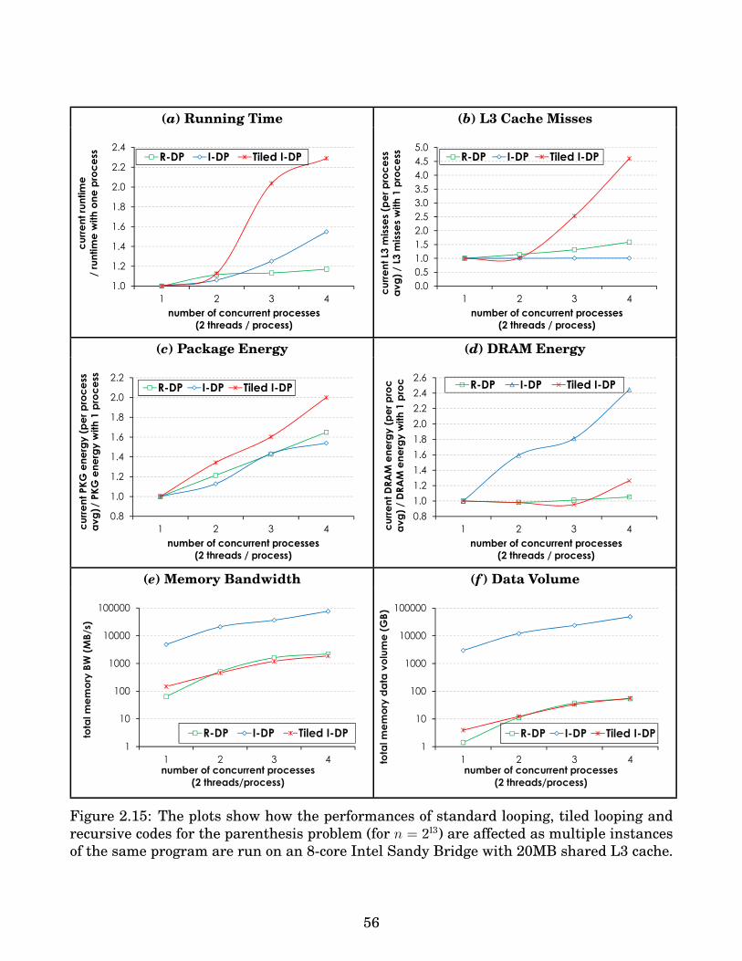
(a) Running Time (b) L3 Cache Misses

1.0

1.2

1.4

1.6

1.8

2.0

2.2

2.4

1 2 3 4

cu

rre

nt

run

tim

e

/ ru

ntim

e w

ith

on

e p

roc

ess

number of concurrent processes

(2 threads / process)


0.0

0.5

1.0

1.5

2.0

2.5

3.0

3.5

4.0

4.5

5.0

1 2 3 4

cu

rre

nt

L3 m

isse

s (p

er

pro

ce

ss

av

g)

/ L3

mis

ses

with

1 p

roc

ess




(c) Package Energy (d) DRAM Energy

0.8

1.0

1.2

1.4

1.6

1.8

2.0

2.2

1 2 3 4cu

rre

nt

PK

G e

ne

rgy

(p

er

pro

ce

ss

av

g)/

PK

G e

ne

rgy

with

1 p

roc

ess




0.8

1.0

1.2

1.4

1.6

1.8

2.0

2.2

2.4

2.6

1 2 3 4cu

rre

nt

DR

AM

en

erg

y (

pe

r p

roc

av

g)

/ D

RA

M e

ne

rgy

with

1 p

roc




(e) Memory Bandwidth (f ) Data Volume

1

10

100

1000

10000

100000

1 2 3 4

tota

l m

em

ory

BW

(M

B/s

)


(2 threads/process)

R-DP I-DP Tiled I-DP1

10

100

1000

10000

100000

1 2 3 4tota

l m

em

ory

da

ta v

olu

me

(G

B)


(2 threads/process)


Figure 2.15: The plots show how the performances of standard looping, tiled looping andrecursive codes for the parenthesis problem (for n = 213) are affected as multiple instancesof the same program are run on an 8-core Intel Sandy Bridge with 20MB shared L3 cache.

56

(a) L3 Cache Misses (b) Running Time

0

50

100

150

200

250

10 20 30 40 50 60 70 80 90 100cu

rre

nt

L3 m

isse

s /

L3 m

isse

s w

ith

en

tire

L3

ca

ch

e a

va

ila

ble

percentage (%) of L3 cache space available

R-DP Tiled I-DP

1

2

3

4

5

6

7

8

10 20 30 40 50 60 70 80 90 100

cu

rre

nt

run

tim

e /

ru

ntim

e w

ith

en

tire

L3

ca

ch

e a

va

ila

ble

percentage (%) of L3 cache space available

R-DP Tiled I-DP

Figure 2.16: The plots show how changes in the available shared L3 cache space affect (a)the number of L3 cache misses, and (b) the serial running time of the tiled looping codeand the recursive code solving the parenthesis problem for n = 213. The code under testwas run on a single core of an 8-core Intel Sandy Bridge processor with 20MB shared L3cache. A multi-threaded Cache Pirate [Eklov et al., 2011] was run on the remaining cores.

2.16 show the results. For lack of space we have included only results for the parenthesisproblem. We have seen similar trends for our other benchmark problems (e.g., FW-APSP).

We have performed experimental analyses of how the performance of a program (R-DP, I-DP, and tiled I-DP) changes if multiple copies of the same program are run on thesame multicore processor (Figure 2.15). We ran up to 4 instances of the same program onan 8-core Sandy Bridge processor with 2 threads (i.e., cores) per process. The block sizeof the tiled code was optimized for best performance with 2 threads. With 4 concurrentprocesses I-DP slowed down by 82% and tiled I-DP by 46%, but R-DP lost only 17% of itsperformance (see Figure 2.15). The slowdown of the tiled code resulted from its inability toadapt to the loss in the shared cache space which increased its L3 misses by a factor of 4(see Figure 2.15). On the other hand, L3 misses incurred by R-DP increased by less thana factor of 2.5. Since I-DP does not have any temporal locality, loss of cache space did notsignificantly change the number of L3 misses it incurred. But I-DP already incurred 90times more L3 misses thanR-DP, and with 4 such concurrent processes the pressure on theDRAM bandwidth increased considerably (see Figure 2.15) causing significant slowdownof the program.

We also report changes in energy consumption of the processes as the number of concur-rent processes increases (Figure 2.15). Energy values were measured using likwid-perfctr

(included in likwid) which reads them from the MSR registers. The energy measurementswere end-to-end (start to end of the program). Three types of energy were measured:package energy which is the energy consumed by the entire processor die, PP0 energy

which is the energy consumed by all cores and private caches, and finally DRAM energy

which is the energy consumed by the directly-attached DRAM. We omitted the PP0 energysince the curves almost always look similar to that of package energy. A single instanceof tiled I-DP consumed 5% less energy than an R-DP instance while I-DP consumed 9times more energy. Average package and PP0 energy consumed by tiled I-DP increased at

57

a faster rate than that by R-DP as the number of processes increased. This happened be-cause both its running time and L3 performance degraded faster than R-DP both of whichcontribute to energy performance. However, since for I-DP L3 misses did not change muchwith the increase in the number of processes, its package and PP0 energy consumptionincreased at a slower rate compared to R-DP’s when number of processes is less than 3.However, as the number of processes increases, energy consumption increases for I-DP ata faster rate, and perhaps because of the DRAM bandwidth contention its DRAM energyincreased significantly.

We have measured the effect on running times and L3 cache misses of serial R-DP andserial tiled I-DP7 when the available shared L3 cache space is reduced (shown in Figure2.16). In this case, the serial tiled-I-DP algorithm was running around 50% faster than theserialR-DP code. The Cache Pirate tool [Eklov et al., 2011] was used to steal cache space8.When the available cache space was reduced to 50%, the number of L3 misses incurred bythe tiled code increased by a factor of 22, but for R-DP the increase was only 17%. Asa result, the tiled I-DP slowed down by over 50% while for R-DP the slowdown was lessthan 3%. Thus R-DP automatically adapts to cache sharing [Bender et al., 2014], but thetiled I-DP does not. This result can be found in the second column of Figure 2.15.

2.8 Conclusion and open problemsWe presented the Autogen algorithm to autogenerate highly efficient recursive algorithmsfor a wide variety of DP problems from their iterative algorithms. We believe that Autogenis the first step towards building a system to automate the process of developing efficientalgorithms for DP problems.

Here are a few open problems:O [Autogen for distributed systems.] Design Autogen to autogenerate R-DP algorithms

for distributed systems.O [Autogen for planar graphs.] The real-life graphs such as routing networks in Inter-

net, transport networks of geographical information systems, and telephone networksare almost planar graphs and it seems possible that we can develop algorithms to ex-ploit temporal locality by working on a localized set of nodes. Design Autogen toautogenerate algorithms for planar graphs.

O [Autogen for r-wayR-DPs.] Design Autogen to autogenerate r-wayR-DPs. Note that,here, r is not a fixed constant but a parameter that can be set at the runtime.

O [Autogen for irregular DPs.] Design Autogen to handle irregular dependencies. E.g.:Viterbi algorithm, knapsack problem, and sieve of Eratosthenes.

O [Autogen for tiled I-DPs.] Design Autogen to autogenerate tiled-iterative DP algo-rithms.

O [Autogen for wavefront I-DPs.] Design Autogen to autogenerate iterative wavefrontDP algorithms.

O [Autogen for partitioned global address space (PGAS) model.] Design Autogen toautogenerate algorithms for the PGAS model.

O [Autogen for graphics processing units (GPUs).] Design Autogen to autogenerate al-gorithms that can be run on GPUs.

7with tile size optimized for best serial performance8Cache Pirate allows only a single program to run, and does not reduce bandwidth.

58

O [Autogen for MapReduce.] Design Autogen to autogenerate algorithms that can useMapReduce.

O [Autogen of Autogen.] Autogen automatically discovers algorithms for a class of prob-lems. Hence, it can be thought of as a level-2 algorithm. What we want is to designa level-2 Autogen or a level-3 algorithm. Is it possible to design an Autogen that canautogenerate Autogens for specific classes of problems and/or hardware?

59

Chapter 3

Semi-Automatic Discovery of EfficientDivide-&-Conquer Wavefront DPAlgorithms

Iterative wavefront algorithms for evaluating dynamic programming recurrences exploitvery high parallelism but show poor cache performance. Tiled-iterative wavefront algo-rithms achieve optimal cache complexity and high parallelism but are cache-aware andhence are not portable and not cache-adaptive. On the other hand, standard cache-obliviousrecursive divide-and-conquer algorithms have optimal serial cache complexity but oftenhave low parallelism due to artificial dependencies among subtasks.

Very recently we introduced cache-oblivious recursive divide-and-conquer wavefront(COW) algorithms that do not have any artificial dependencies, but they are too compli-cated to develop, analyze, implement, and generalize. Though COW algorithms are basedon fork-join primitives, they extensively use atomic operations for ensuring correctness,and as a result, performance guarantees (i.e., parallel running time and parallel cache com-plexity) provided by state-of-the-art schedulers (e.g., the randomized work-stealing sched-uler) for programs with fork-join primitives do not apply. Also extensive use of atomic locksmay result in high overhead in implementation.

In this chapter, we show how to systematically transform standard cache-oblivious re-cursive divide-and-conquer algorithms into recursive divide-and-conquer wavefront algo-rithms to achieve optimal parallel cache complexity and high parallelism under state-of-the-art schedulers for fork-join programs. Unlike COW algorithms these new algorithms donot use atomic operations. Instead they use timing functions to compute at what time eachdivide-and-conquer function must be launched in order to achieve high parallelism withoutlosing cache performance. The resulting implementations are arguably much simpler thanthose of known COW algorithms. We present theoretical analyses and experimental per-formance and scalability results showing superiority of these new algorithms over existingalgorithms.

3.1 IntroductionFor good performance on a modern multicore machine with a cache hierarchy, algorithmsmust have good parallelism and should be able to use the caches efficiently at the same

60

time. Iterative wavefront algorithms for solving DP problems have optimal parallelismbut often suffer due to bad cache performance. On the other hand, though standard cache-oblivious [Frigo et al., 1999] recursive divide-and-conquer DP algorithms have optimalserial cache complexity, they often have low parallelism. The tiled-iterative wavefrontalgorithms achieve optimality in cache complexity and achieve high parallelism but arecache-aware, and hence are not portable and do not adapt well when available cache spacefluctuates during execution in a multiprogramming environment. Very recently, the cache-oblivious wavefront (COW) algorithms [Tang et al., 2015] have been proposed that have op-timal parallelism and optimal serial cache complexity. However, though those algorithmsare based on fork-join primitives, they extensively use atomic operations for correctness.But current theory of scheduling nested parallel programs with fork-join primitives do notallow such atomic operations. As a result, no bounds on parallel running time and parallelcache complexity could be proved for those algorithms. Those algorithms are also very dif-ficult to implement since they require hacking into a parallel runtime system. Extensiveuse of atomic locks causes too much overhead for very large and higher dimensional DPs.

In this chapter, we present a provably efficient method for scheduling cache-obliviousrecursive divide-and-conquer wavefront algorithms on a multicore machine which opti-mizes parallel cache complexity and achieves high parallelism. Our algorithms are basedon fork-join primitives, but do not use atomic operations. As a result, we are able to analyzetheir parallel running times and parallel cache complexities easily under state-of-the-artschedulers for fork-join based parallel programs. Our algorithms are also much simpler toimplement compared to COW algorithms.

Iterative algorithms. Traditionally, DP algorithms are implemented iteratively using aseries of (nested) loops and they can be parallelized easily. They are called I-DPs. Thesealgorithms often have good spatial locality, no temporal locality, and standard implemen-tations may not have optimal parallelism as well. For example, an iterative algorithm forthe parenthesis problem (explained in Section 2.2) has T∞(n) = Θ (n2) and Q1(n) = Θ (n3).

Iterative algorithms are also implemented as tiled loops, in which case the entire DPtable is blocked or tiled and the tiles are executed iteratively. They are called T I-DPs.For example, for a tiled iterative algorithm for the parenthesis problem with r × r tilesize, where r ∈ [2, n], we have T∞(n) = Θ ((n/r)2) · Θ (r2) = Θ (n2), and Q1(n, r) = (n/r)3 ·O (r2/B + r) = O (n3/(rB) + n3/r2).

Fastest iterative DP implementations have the following wavefront-like property. Saya cell x in a DP table is written by reading from the cell 〈y1, y2, . . . , ys〉. When the cellsy1, y2, . . . , ys are completely updated, then the cell x can immediately get updated, eitherpartially or fully. This property leads to the computation of a DP table in a wavefrontmanner. We call wavefront iterative algorithmsWI-DPs. For example, for the parenthesisproblem, an iterative wavefront algorithm has the shortest span of T∞(n) = Θ (n log n), buthas the worst possible cache complexity of Q1(n) = O (n3). The Θ (log n) factor in the spancomes from the parallel for construct.

Recursive divide-and-conquer algorithms. Cache-oblivious recursive divide-and-conquerparallel DP algorithms can overcome many of the limitations of their iterative counter-parts. While iterative algorithms often have poor or no temporal locality, recursive algo-rithms have excellent and often optimal temporal locality. One problem with recursivedivide-and-conquer algorithms is that they trade off parallelism for cache optimality, and

61

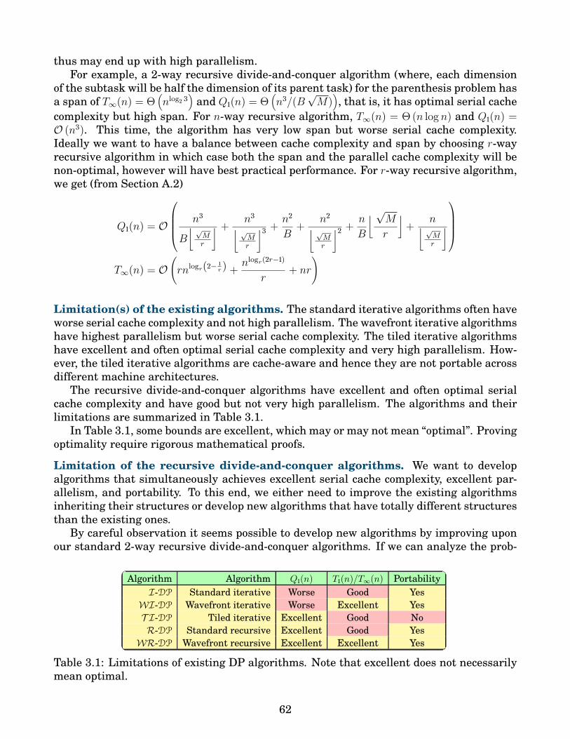
thus may end up with high parallelism.For example, a 2-way recursive divide-and-conquer algorithm (where, each dimension

of the subtask will be half the dimension of its parent task) for the parenthesis problem hasa span of T∞(n) = Θ

(nlog2 3

)and Q1(n) = Θ

(n3/(B

√M)

), that is, it has optimal serial cache

complexity but high span. For n-way recursive algorithm, T∞(n) = Θ (n log n) and Q1(n) =O (n3). This time, the algorithm has very low span but worse serial cache complexity.Ideally we want to have a balance between cache complexity and span by choosing r-wayrecursive algorithm in which case both the span and the parallel cache complexity will benon-optimal, however will have best practical performance. For r-way recursive algorithm,we get (from Section A.2)

Q1(n) = O

n3

B⌊ √

Mr

⌋ + n3⌊ √Mr

⌋3 + n2

B+ n2⌊ √

Mr

⌋2 + n

B

⌊ √M

r

⌋+ n⌊ √

Mr

⌋

T∞(n) = O(rnlogr(2− 1

r ) + nlogr(2r−1)

r+ nr

)

Limitation(s) of the existing algorithms. The standard iterative algorithms often haveworse serial cache complexity and not high parallelism. The wavefront iterative algorithmshave highest parallelism but worse serial cache complexity. The tiled iterative algorithmshave excellent and often optimal serial cache complexity and very high parallelism. How-ever, the tiled iterative algorithms are cache-aware and hence they are not portable acrossdifferent machine architectures.

The recursive divide-and-conquer algorithms have excellent and often optimal serialcache complexity and have good but not very high parallelism. The algorithms and theirlimitations are summarized in Table 3.1.

In Table 3.1, some bounds are excellent, which may or may not mean “optimal”. Provingoptimality require rigorous mathematical proofs.

Limitation of the recursive divide-and-conquer algorithms. We want to developalgorithms that simultaneously achieves excellent serial cache complexity, excellent par-allelism, and portability. To this end, we either need to improve the existing algorithmsinheriting their structures or develop new algorithms that have totally different structuresthan the existing ones.

By careful observation it seems possible to develop new algorithms by improving uponour standard 2-way recursive divide-and-conquer algorithms. If we can analyze the prob-

Algorithm Algorithm Q1(n) T1(n)/T∞(n) PortabilityI-DP Standard iterative Worse Good Yes

WI-DP Wavefront iterative Worse Excellent YesT I-DP Tiled iterative Excellent Good NoR-DP Standard recursive Excellent Good Yes

WR-DP Wavefront recursive Excellent Excellent Yes

Table 3.1: Limitations of existing DP algorithms. Note that excellent does not necessarilymean optimal.

62

lem behind not very high parallelism for recursive divide-and-conquer algorithms and solvethat problem, it seems that we can develop new algorithms.

The low parallelism in 2-way recursive divide-and-conquer algorithms results from ar-tificial dependencies among subproblems that are not implied by the underlying DP recur-rence [Tang et al., 2015].

A 2-way recursive divide-and-conquer algorithm for the LCS problem splits the DP ta-ble X into four equal quadrants: X11 (top-left), X12 (top-right), X21 (bottom-left), and X22(bottom-right). It then recursively computes the quadrants in the following order: X11 first,then X12 and X21 in parallel, and finally X22. As per the recursive structure, the top-leftquadrant of X12 and X21 i.e., X12,11 and X21,11, respectively, can only start executing whenthe execution of the bottom-right quadrant of X11 i.e., X11,11 completes. This dependency be-tween subproblems or subtasks is not defined by the underlying DP recurrence but definedby the recursive structure of the algorithm. Such dependencies in a recursive algorithmare called artificial dependencies. There are artificial dependencies at several differentgranularities. Most often, these artificial dependencies asymptotically increase the spanthereby reducing parallelism. By removing such artificial dependencies but retaining therecursive structure we can design algorithms to achieve high parallelism.

Recursive divide-and-conquer wavefront algorithms. The 2-way recursive algo-rithms have optimal serial cache complexity and not very high parallelism. On the otherhand, the wavefront iterative algorithms have high parallelism and worse cache complex-ity. Is it possible to inherit the best features from both the worlds? Yes.

By removing artificial dependencies from the recursive algorithms, it is possible todevelop algorithms that simultaneously achieve excellent cache-locality, excellent paral-lelism, and cache-obliviousness. Such algorithms are called recursive wavefront or divide-and-conquer wavefront or cache-oblivious wavefront algorithms.

Recursive wavefront algorithms were introduced in [Tang et al., 2015]. Such algorithmskeep several processors busy-waiting and hence wastes CPU resources. Also, those algo-rithms are too complicated to develop, analyze, implement, and generalize. Atomic in-structions were used extensively to identify and launch ready tasks, and implementationsrequired hacking into Cilk’s runtime system. No bounds on parallel cache complexities ofthose algorithms are known.

The Autogen-Wave framework and scheduling algorithms. In this chapter, we presenta framework called Autogen-Wave to discover recursive wavefront algorithms based on tim-ing functions. These algorithms have a structure similar to the standard recursive divide-and-conquer algorithms, but each recursive function call is annotated with start-time andend-time hints that are passed to the scheduler. Timestamps represent the relative time atwhich a task starts or ends execution. Closed-form formulas or functions to get the exacttimestamps at which different recursive functions write to different regions of the DP tableare found. Such closed-form formulas or functions to compute the timestamps are pluggedinto the recursive algorithm for all the function invocations to derive a recursive wavefrontalgorithm.

The performance of a parallel algorithm does not depend on the algorithm alone, it alsodepends on the scheduler that schedules different threads to work on different processors.The recursive wavefront algorithms make use of timestamps and existing schedulers do notunderstand timestamps. Hence, we present a space-efficient scheduling method to attain

63

A(X,X,X)

1. if X is a cell then Acell(X,X,X)2. else3. parallel: A(X11, X11, X11), A(X22, X22, X22)4. B(X12, X11, X22)

B(X,U, V )

1. if X is a cell then Bcell(X,U, V )2. else3. B(X21, U22, V11)4. parallel: C(X11, U12, V21), C(X22, X21, V12)5. parallel: B(X11, U11, V11), B(X22, X22, V22)6. C(X12, U12, X22)7. C(X12, X11, V12)8. B(X12, U11, V22)

C(X,U, V )

1. if X is a cell then Ccell(X,U, V )2. else3. parallel: C(X11, U11, V11), C(X12, U11, V12),

C(X21, U21, V11), C(X22, U21, V12)4. parallel: C(X11, U12, V21), C(X12, U12, V22),

C(X21, U22, V21), C(X22, U22, V22)

Programmer computesthe timing functions

SA (X,X,X)

1. return C(xr, xc)

SB (X,U, V )

1. return C(xr + n− 1, xc)

SC (X,U, V )

1. m← (xr + n− 1 + xc)/2; u← uc + n− 12. if uc > m then return max C(ur + n− 1, uc),C(uc, xc)+13. elif u < m then return max C(ur + n− 1, u),C(u, xc)+ 14. else return

(max C(ur + n− 1,m),C(m,xc)+ 1).[uc > (xr + xc)/2]

EA (X,X,X)

1. return C(xr, xc +n−1)

EB (X,U, V )

1. return C(xr, xc +n−1)

EC (X,U, V )

1. lval← max C(ur, uc),C(uc, xc + n− 1)2. rval← max C(ur, uc + n− 1),C(uc + n− 1, xc + n− 1)3. return (max lval, rval+ 1).[uc > (xr + xc)/2]

C(i, j)

1. if (j− i) ≤ 1 then return (j− i) else return 2× (j− i)− 1

Transformation by thescheduler / programmer

RECURSIVE-WAVEFRONT-PARENTHESIS()

1. w ← 02. while w <∞ do w ← A(G,G,G,w)

A(X,X,X,w)

1. vi ←∞ for all i ∈ [1, 3]2. if X is an n′ × n′ matrix then3. if w = SA (X,X,X) then Achunk(X,X,X)4. else5. F1..3 ← A,A,B6. arg1..3 ← (X11, X11, X11), (X22, X22, X22),

(X12, X11, X22)7. parallel for i← 1 to 3 do8. if w < SFi

(argi) then vi ← SFi(argi)

9. elif w ≤ EFi(argi) then vi ← Fi(argi, w)

10. sync11. return min vi for all i ∈ [1, 3]

B(X,U, V,w)

1. vi ←∞ for all i ∈ [1, 8]2. if X is an n′ × n′ matrix then3. if w = SB (X,U, V ) then Bchunk(X,U, V )4. else5. F1..8 ← B,C,C,B,B,C,C,B6. arg1..8 ← (X21, U22, V11), (X11, U12, V21),

(X22, X21, V12), (X11, U11, V11),(X22, X22, V22), (X12, U12, X22),(X12, X11, V12), (X12, U11, V22)

7. parallel for i← 1 to 8 do8. if w < SFi




C(X,U, V,w)

1. vi ←∞ for all i ∈ [1, 8]2. if X is an n′ × n′ matrix then3. if w = SC (X,U, V ) then Cchunk(X,U, V )4. else5. F1..8 ← C,C,C,C,C,C,C,C6. arg1..8 ← (X11, U11, V11), (X12, U11, V12),

(X21, U21, V11), (X22, U21, V12),(X11, U12, V21), (X12, U12, V22),(X21, U22, V21), (X22, U22, V22)





Figure 3.1: Left: The programmer derives the timing functions from a given standard 2-way recursive divide-and-conquer DP algorithm for the parenthesis problem. A region Zhas its top-left corner at (zr, zc) and is of size n× n. Right: A recursive divide-and-conquerwavefront algorithm is generated for the parenthesis problem. The programmer derivesthe algorithm if work-stealing scheduler (see Section 3.4.1) is used and the scheduler de-rives the algorithm if W-SB scheduler (see Section 3.4.2) is used. The algorithm makes useof the timing functions derived by the programmer.

excellent parallel cache complexity and very high parallelism. Our approach makes use ofa combination of ideas from space-bounded scheduler and scheduling based on timestamps.

64

We also analyze the complexities under a randomized work-stealing scheduler.Our task schedulers make sure that the algorithms are executed in a wavefront fash-

ion using the timing functions. Indeed, the transformation the scheduler is expected todo based on the timing functions is straightforward, and a programmer may choose todo that herself and use a scheduler that do not accept hints. The transformed code isstill purely based on fork-join parallelism, and the performance bounds (e.g., parallel run-ning time and parallel cache complexity) guaranteed by any scheduler supporting fork-joinparallelism apply. The recursive wavefront algorithm for the parenthesis problem hasT∞(n) = Θ (n log n) and Q1(n) = O

(n3/(B

√M)

). The bounds on Tp and Qp can be obtained

from the scheduler guarantees.The theoretical performance of several algorithms for the parenthesis problem are sum-

marized in Table 3.2. In the table, I-DP represents standard iterative, T I-DP representstiled iterative, WI-DP represents iterative wavefront, R-DP represents recursive divide-and-conquer, andWR-DP recursive divide-and-conquer wavefront algorithms.

Related work. The tiled iterative algorithms [Wolf, 1992,Darte et al., 1997,Panda et al.,1999, Sarkar and Megiddo, 2000, Goumas et al., 2001, Renganarayanan et al., 2012] havebeen studied extensively as tiling is the traditional way of implementing dynamic pro-gramming and other matrix algorithms. There are several frameworks to automaticallyproduce tiled codes such as PLuTo [Bondhugula et al., 2008], Polly [Grosser et al., 2012],and PoCC [Pouchet et al., 2010]. However, these softwares are not designed to generatecorrect parallel tiled code for non-trivial DP recurrences. The major concerns with tiledprograms are that they are cache-aware and sometimes processor-aware that sacrificesportability across machines. Another disadvantage of being cache-aware is that the al-gorithms are not cache-adaptive [Bender et al., 2014], i.e., the algorithms do not adaptto changes in available cache/memory space during execution and hence may run slowerwhen multiple programs run concurrently in a shared-memory environment [Chowdhuryet al., 2016b]. For example in applications such as cloud technologies and virtual networksin data centers, available memory changes continuously.

Several existing systems such as Bellman’s GAP compiler [Giegerich and Sauthoff,2011], semi-automatic synthesizer [Pu et al., 2011], EasyPDP [Tang et al., 2012], EasyHPS[Du et al., 2013], pattern-based system [Liu and Schmidt, 2004], and parallelizing plug-ins [Reitzig, 2012] can be used to generate iterative and tiled loop programs. Parallel taskgraph execution systems such as Nabbit [Agrawal et al., 2010] and BDDT [Tzenakis et al.,2013] execute the DP tasks during runtime using unrolling. Due to this they might losecache efficiency.

The classic 2-way recursive divide-and-conquer algorithms having optimal serial cachecomplexity and good (but, not always optimal) parallelism have been developed, analyzed,and implemented in [Chowdhury and Ramachandran, 2008, Chowdhury and Ramachan-dran, 2010], [Tithi et al., 2015]. Hybrid r-way algorithms are considered in [Chowdhuryand Ramachandran, 2008] but they are either cache- or processor-aware and complicatedto program. Pochoir [Tang et al., 2011] is used to generate cache-oblivious implementationsto stencils. However, the recursive algorithms often have low parallelism due to artificialdependencies among subtasks. Recently Aga et al. [Aga et al., 2015] proposed a speculationapproach to alleviate the concurrency constraints imposed by the artificial dependencies instandard parallel recursive divide-and-conquer programs and reported a speedup up to1.6× on 30 cores over their baseline.

65

Algorithm Sch. Q1(n) T∞(n) Qopt1 (n) Qopt

p (n) High par.I-DP WS O (n3) Θ (n2) 7 7 7

r-size T I-DP WS O (n3/(rB) + n3/r2) Θ (n2) 7 7 7√M -size T I-DP WS O

(n3/(B

√M) + n3/M

)Θ (n2) 3 7 7

WI-DP WS O (n3) Θ (n log n) 7 7 3

2-way R-DP WS O(n3/(B

√M)

)Θ(nlog2 3

)3 7 7

r-way R-DP WS O

n3/(Bb√M/rc

)+ n3/

(b√M/rc3

) O(rnlogr(2− 1

r ) + nr

+ (1/r)nlogr(2r−1)

)7 7 7

WR-DP WS O(n3/(B

√M)

)Θ (n log n) 3 − 3

*WR-DP WS O(n3/(B

√M)

)Θ (n log n) 3 3 3

*WR-DP W-SB* O(n3/(B

√M)

)Θ (n log n) 3 3 3

Table 3.2: Different DP algorithms to solve the parenthesis problem using various sched-ulers. In the r-way R-DP, r is a constant. The second column represents the schedulers:WS means work stealing, W-SB means modified space bounded. * represents the algo-rithms presented in this chapter. The last column means excellent parallelism. In thelast three columns, we use 3 to denote optimality or near-optimality and “−” to denotenon-applicability.

The recursive wavefront algorithms were introduced in [Tang et al., 2015] but they aretoo complicated to develop, analyze, implement, and generalize. They make extensive useof atomic instructions, and standard analysis model of fork-join parallelism does not apply.In this paper we try to address these issues.

Our contributions. Our major contributions are as follows:(1) [Framework.] We present a framework called Autogen-Wave to discover recursive

divide-and-conquer wavefront algorithms based on timing functions. The recursivewavefront algorithms are superior to all existing algorithms for DP problems.

(2) [Divide-and-conquer wavefront algorithms.] We present several recursive divide-and-conquer wavefront algorithms derived using the Autogen-Wave framework.

(3) [Schedulers.] We also present two scheduling methods to schedule a a recursive wave-front algorithm: (i) the algorithm passes timing functions and space usage info tomodified version of a hint-accepting space-bounded scheduler, (ii) the programmerappropriately transforms the algorithm to use the timing functions, and uses a stan-dard randomized work-stealing scheduler to run the program.

Organization of the chapter. In Section 3.2, we present our Autogen-Wave frameworkthat can be used to discover recursive wavefront algorithms based on timing functions. Twoschedulers to schedule recursive wavefront algorithms and their analysis are presented inSection 3.4.

3.2 The Autogen-Wave frameworkIn this section, we present a framework called Autogen-Wave that can be used to derive arecursive divide-and-conquer wavefront algorithm from a standard recursive divide-and-conquer DP algorithm. The method involves augmenting all recursive function calls withtiming functions to launch them as early as possible without violating any dependency

66

R-DP WR-DP

Work Serial cache Span Best serial cache Best spanProblem (T1) comp. (Q1) (T∞) comp. (Q1) (T∞)Parenthesis problem Θ (n3) Θ

(n3/(B

√M)

)Θ(nlog 3

)Θ(n3/(B

√M)

)Θ (n log n)

Floyd-Warshall’s APSP 3-D Θ (n3) Θ (n3/B) Θ(n log2 n

)Θ (n3/B) Θ (n log n)

Floyd-Warshall’s APSP 2-D Θ (n3) Θ(n3/(B

√M)

)Θ(n log2 n

)Θ(n3/(B

√M)

)Θ (n log n)

LCS / Edit distance Θ (n2) Θ (n2/(BM)) Θ(nlog 3

)Θ (n2/(BM)) Θ (n log n)

Gap problem Θ (n3) Θ(n3/(B

√M)

)Θ(nlog 3

)Θ(n3/(B

√M)

)Θ (n log n)

3-point stencil Θ (n2) Θ (n2/(BM)) Θ(nlog 3


Protein accordion folding Θ (n3) Θ(n3/(B

√M)

)Θ (n log n) Θ

(n3/(B

√M)

)Θ (n log n)

Spoken-word recognition Θ (n2) Θ (n2/(BM)) Θ(nlog 3


Function approximation Θ (n3) Θ(n3/(B

√M)

)Θ(nlog 3

)Θ(n3/(B

√M)

)Θ (n log n)

Binomial coefficient Θ (n2) Θ (n2/(BM)) Θ(nlog 3


Bitonic traveling salesman Θ (n2) Θ (n2/(BM)) Θ (n log n) Θ (n2/(BM)) Θ (n log n)

Table 3.3: Work (T1), serial cache complexity (Q1), and span (T∞) of R-DP and WR-DP

algorithms for several DP problems. Here, n = problem size, M = cache size, B =block size, and p = #cores. We assume that the DP table is too large to fit into thecache, and M = Ω

(Bd)

when Θ(nd)

is the size of the DP table. On p cores, the run-ning time is Tp = O (T1/p+ T∞). The R-DP algorithms have a parallel cache complexityis Qp = O (Q1 + p(M/B)T∞) with high probability when run under the randomized work-stealing scheduler on a parallel machine with private caches. The WR-DP algorithmshave a parallel cache complexity of Qp = O (Q1) when run with the modified space-boundedscheduler.

constraints implied by the DP recurrence. The timing functions are derived analytically,and do not employ locks or atomic instructions.

Our transformation allows the updates to the DP table proceed in an order close toiterative wavefront, but from within the structure of a recursive divide-and-conquer algo-rithm. The goal is to reach the higher parallelism of an iterative wavefront algorithm whileretaining the better cache performance (i.e., efficiency and adaptivity) and portability (i.e.,cache- and processor-obliviousness) of a recursive algorithm.

We had defined I-DP and R-DP in Section 2.2. Here, we define a more terms that wewill use throughout the chapter.

Definition 19 (T I-DP/WI-DP). Let P be a given DP problem. Then, a T I-DP is a par-allel tiled iterative algorithm for solving P and WI-DP is a parallel wavefront iterativealgorithm for P.

Typically a T I-DP is autogenerated from a polyhedral compiler (parallelizer and local-ity optimizer) such as Pluto. These T I-DPs will not have the highest parallelism. On theother hand,WI-DPs have the highest parallelism.

Definition 20 (WR-DP/Autogen-Wave). Let P be a given DP problem. A WR-DP is arecursive wavefront algorithm for P. Autogen-Wave is our framework that can be used toderive aWR-DP from a given R-DP and its corresponding DP recurrence.

Autogen-WaveR-DP WR-DP

67

Let us first define the wavefront order of applying updates to a DP table. Each updatewrites to one DP table cell by reading values from other cells. An update becomes readywhen all cells it reads from are fully updated. We assume that only ready updates canbe applied and each such update can only be applied once. A wavefront order of updatesproceeds in discrete timesteps. In each step all ready updates to distinct cells are applied inparallel. However, if a cell has multiple ready updates only one of them is applied, and therest are retained for future. A wavefront order does not have any artificial dependencies.

The Autogen-Wave framework. The Autogen-Wave framework consists of three majorsteps:

(1) [Completion-time function construction.] A closed-form formula or function (that canbe evaluated in constant time) is derived based on the original DP recurrence thatgives the timestep at which each DP cell is fully updated in wavefront order. SeeSection 3.2.1.

(2) [Start- and end-time functions construction.] Cell completion times are used to deriveclosed-form formulas that give the timesteps in wavefront order at which each recur-sive function call should start and end execution. See Section 3.2.2.

(3) [Divide-and-conquer wavefront algorithm derivation.] Each recursive function call inthe standard recursive algorithm is augmented with its start- and end-time functionsso that the algorithm can be used to apply only the updates in any given timestep inwavefront order. We then use a variant of iterative deepening on top of this recursivealgorithm to execute all timesteps efficiently. See Section 3.2.3.

We describe our transformation for arbitrary d-dimensional (d ≥ 1) DP in which eachdimension of the DP table is of the same length and is a power of 2.

Example. We explain our approach by applying it on an R-DP algorithm for the paren-thesis problem [Cherng and Ladner, 2005], which is defined as follows. Let G[i, j] denotethe minimum cost of parenthesizing si · · · sj. Then the 2D DP table G[0 : n, 0 : n] is filled upusing the following recurrence:

G[i, j] =


G[i, k] + G[k, j] + w(i, k, j) if 0 ≤ i < j − 1 < n;(3.1)

where the vj ’s and function w(·, ·, ·) are given. The recurrence is evaluated by the recursivealgorithm [Tithi et al., 2015] given at the top of Figure 3.1. In the rest of the section, weshow how a recursive wavefront algorithm (shown in Figure 3.1) can be derived from thegiven algorithm.

Fundamentals. We need to understand the fundamental concepts of timestamps, timesteps and races before understanding the Autogen-Wave framework.

Definition 21 (Timestamp). A timestamp, denoted by Ft(x, y1, . . . , ys), is an update by aproblem-specific function F writing to the cell x reading information from the cells y1, . . . , ysat time t.

Sometimes we also specify time in the form of t.t′, where the term t′ is used to avoidrace conditions. If there are multiple updates that read information from different sets ofcells and write to the same cell at the same time there will be race. Each such update willbe performed at the same t value, but different t′ values. We do not require t′ for standard

68

iterative and recursive algorithms. For fast iterative algorithm it becomes easier to findpatterns if we use t′.

For the parenthesis problem, the timestamps (without t′ term) for I-DP,R-DP,WI-DP,andWR-DP algorithms are given in Table 3.4. The right column of the table gives the lastupdated timestep for each cell of the DP table for different algorithms.

Consider the standard 2-way recursive algorithm for the parenthesis problem given inthe top-left corner of Figure 3.1. It has three functions that update the DP table. Initially,function A(G,G,G) is called, where G is the entire DP table. Then the computation pro-gresses by recursively breaking the table into quadrants, and calling functions A, B andC on these smaller regions of G. At the base case (i.e., a 1 × 1 region of G), each functionupdates a cell. When x is a cell, function A(x, x, x) updates x by reading x itself whichcorresponds to the case i = k = j in the recurrence. Similarly, function B(x, u, v) updatescell x by reading x itself and two other cells u and v which correspond to cases i = k , jand i , k = j. Finally, function C(x, u, v) updates the cell x by reading the two cells u and vwhich corresponds to i , k , j.

The middle part of Table 3.4 shows how the standard 2-way recursive algorithm with1× 1 base case updates G[1 : n, 1 : n] when n = 8. We use Ft in a cell to denote that functionF updates the cell at timestep t, where F ∈ A,B,C. Using an unbounded number ofprocessors the standard recursive algorithm updates the entire table in 31 timesteps. Incontrast, the bottom part of Table 3.4 shows that an iterative wavefront algorithm willupdate G in only 18 timesteps.

The top part of the Table 3.4 shows how I-DP updates an 8×8 DP table in 28 timesteps.And the R-DP takes 31 timesteps to update the DP table. However, the span of I-DP isΘ (n2) and that of R-DP is Θ

(nlog 3

). For much larger DP tables it becomes clear that I-DP

takes many more timesteps than R-DP to update the entire DP table.It is important to note the we have used three functions A,B,C for the updates of the it-

erative algorithms. Each function has a specific functionality as described in the precedingparagraphs.

With a 1 × 1 base case the WR-DP algorithms will perform the updates in exactly thesame order as theWI-DP algorithm, and terminate in 18 steps. The timestamps are shownin the bottom part of Table 3.4.

Our goal is to derive a recursive divide-and-conquer wavefront algorithm that hastimestamps identical to a fast iterative algorithm.

3.2.1 Completion-time function constructionIn this section, we define completion-time, and show how to compute it in O (1) time forany cell.

Definition 22 (Completion-time). The completion-time for a particular cell x, denoted byC(x), is the timestep in wavefront order at which x is fully updated. More formally,

C(x) = max t | for all Ft(x, . . .); (3.2)

where Ft(x, . . .) means that cell x is updated by function F at timestep t.

Completion-time of a cell computed from the given DP recurrence is as follows.

69

A0 B1 C2B3 C4C5B6 C7C8C9B10 C11C12C13C14B15 C16C17C18C19C20B21 C22C23C24C25C26C27B28− A0 B1 C2B3 C4C5B6 C7C8C9B10 C11C12C13C14B15 C16C17C18C19C20B21− − A0 B1 C2B3 C4C5B6 C7C8C9B10 C11C12C13C14B15− − − A0 B1 C2B3 C4C5B6 C7C8C9B10− − − − A0 B1 C2B3 C4C5B6− − − − − A0 B1 C2B3− − − − − − A0 B1− − − − − − − A0

0 1 3 6 10 15 21 28− 0 1 3 6 10 15 21− − 0 1 3 6 10 15− − − 0 1 3 6 10− − − − 0 1 3 6− − − − − 0 1 3− − − − − − 0 1− − − − − − − 0

I-DP


0 1 4 7 18 21 28 31− 0 2 4 16 18 26 28− − 0 1 10 13 18 21− − − 0 8 10 16 18− − − − 0 1 4 7− − − − − 0 2 4− − − − − − 0 1− − − − − − − 0

R-DP


0 1 3 6 9 12 15 18− 0 1 3 6 9 12 15− − 0 1 3 6 9 12− − − 0 1 3 6 9− − − − 0 1 3 6− − − − − 0 1 3− − − − − − 0 1− − − − − − − 0

WI-DP &WR-DP

Table 3.4: Left: Timesteps at which each DP table cell is updated (Ft means function F updatesat timestep t). Right: Timesteps at which each cell becomes fully updated (on the right) for theparenthesis problem on a DP table of size 8 × 8. Top: standard I-DP which has a span of Θ

(n2).

Middle: standard 2-way R-DP algorithm which has a span of Θ(nlog 3

). Bottom: WI-DP andWR-

DP algorithms which has a span of Θ (n log n) overall (including traversing the recursion tree) butjust Θ (n) to update the DP table. All recursive algorithms use a 1 × 1 base case. We assume thatthe number of processors is unbounded.

A0.0 B1.0 C2.0B3.0 C4.0C4.1B5.0 C4.0C6.0C6.1B7.0 C6.0C6.1C8.0C8.1B9.0 C6.0C8.0C8.1C10.0C10.1B11.0 C8.0C8.1C10.0C10.1C12.0C12.1B13.0− A0.0 B1.0 C2.0B3.0 C4.0C4.1B5.0 C4.0C6.0C6.1B7.0 C6.0C6.1C8.0C8.1B9.0 C6.0C8.0C8.1C10.0C10.1B11.0− − A0.0 B1.0 C2.0B3.0 C4.0C4.1B5.0 C4.0C6.0C6.1B7.0 C6.0C6.1C8.0C8.1B9.0− − − A0.0 B1.0 C2.0B3.0 C4.0C4.1B5.0 C4.0C6.0C6.1B7.0− − − − A0.0 B1.0 C2.0B3.0 C4.0C4.1B5.0− − − − − A0.0 B1.0 C2.0B3.0− − − − − − A0.0 B1.0− − − − − − − A0.0

Table 3.5: The timestamps for the parenthesis problem for a DP table size 8 × 8 using a WR-DP

algorithm.

C(x) =

initial values initial conditions,smax(x) + flag(x) + su(x) otherwise;

(3.3)

where smax(x) is the maximum completion time of the cells on which x directlydepends, i.e., smax(x) = maxF(x,...,y,...) C(y) and y , x; flag(x) = 0 if the cell-tuple(with maximum completion-time as smax(x)) is inflexible and flag(x) = 1 if the cell-tuple is flexible; and the term su(x) is 1 if there is a self-update function that readsfrom itself; and 0, otherwise.

In simple words, the last timestep at which a cell is updated/written is called thecompletion-time of that cell. The term smax(x) is the maximum completion-time of all

70

possible read cells of the cell x. The letter s in smax means start-time. It means that thecell x gets completed only after all of its read cells are started and finish their execution.This is also the reason to include the term 1. The term su(x) is required to avoid collisionsor race conditions. The idea for self-update function was given by Jesmin Jahan Tithi.

We need to find closed-form formulas to find the completion-time of the WR-DP algo-rithm. The timestamps of theWR-DP algorithm for all cells of an 8× 8 DP table is shownin Table 3.5. The completion-time for any cell (i, j) in the DP table can be found as follows.

C(i, j) =

0 if i = j,

C(i, j − 1) + 0 + 1 if i = j − 1,C(i, j − 1) + 1 + 1 if i <= j − 2;

(3.4)

because smax(i, j) = C(i, j − 1) = C(i + 1, j); if i ≤ j − 1, then su(i, j) = 1 as the self-updatefunction B updates the cell (i, j) reading from itself. When i = j − 1, there is no cell-tuplethat does not read from (i, j) and when i ≤ j− 1, there is at least one flexible tuple. Solvingthe recurrence, we get the following:

C(i, j) =

j − i if (j − i) = 0,2(j − i)− 1 if (j − i) ≥ 1.

(3.5)

3.2.2 Start-time and end-time functions construction

In this section, we define start-time and end-time for a recursive function call, and showhow to derive them from completion-times.

In an R-DP, every function invokes one or more recursive functions. Each function callwill only be executed when all its read regions are completely updated. On the other hand,in a WR-DP, a function will be executed when as soon as a single cell of the write regionis ready to execute. The relative timestep at which a function starts execution is calledstart-time and the relative timestep when the function completes execution is termed end-time. Closed-form formulas / mathematical functions are constructed to find the start- andend-times.

Definition 23 (Start-time and end-time). The start-time (resp. end-time) of a recursivefunction call in aWR-DP algorithm is the earliest (resp. latest) timestep in wavefront orderat which one of the updates to be applied by that function call (either directly or through arecursive function call) becomes ready.

Let F(X, Y1, . . . , Ys) be a function call that writes to a region X by reading from re-gions Y1, . . . , Ys of the DP table. Its start- and end-times, denoted by SF (X, Y1, . . . , Ys) andEF (X, Y1, . . . , Ys), respectively, are computed as follows.

71

SF (X, Y1, . . . , Ys)︸︷︷︸X∈Y1,...,Ys

=

(C(X)).0 if X is a cell,min SF′ (X ′, Y ′1 , . . . , Y ′s ) otherwise;

(3.6)

SF (X, Y1, . . . , Ys)︸︷︷︸X<Y1,...,Ys

=

(min1≤i≤sC(Yi)+ 1).ra(X, Y1, . . . , Ys) if X is a cell,min SF′ (X ′, Y ′1 , . . . , Y ′s ) otherwise;

(3.7)

EF (X, Y1, . . . , Ys)︸︷︷︸X∈Y1,...,Ys

=

(C(X)).0 if X is a cell,max EF′ (X ′, Y ′1 , . . . , Y ′s ) otherwise;

(3.8)

EF (X, Y1, . . . , Ys)︸︷︷︸X<Y1,...,Ys

=

(max1≤i≤sC(Yi)+ 1).ra(X, Y1, . . . , Ys) if X is a cell,max EF′ (X ′, Y ′1 , . . . , Y ′s ) otherwise;

(3.9)

where, in the non-cellular case minimization/maximization is taken over all functionsF′(X ′, Y ′1 , . . . , Y ′s ) recursively called by F(X, Y1, . . . , Ys). Also, ra(X, Y1, . . . , Ys) is the problem-specific race avoidance condition used when two functions write to the same region. Thoughwe use real-valued timesteps for simplicity, the total number of distinct timesteps remainexactly the same as that in theWI-DP algorithm.

For the parenthesis problem, the start-times for the three functions A,B, and C arecomputed as below. Let (xr, xc), (ur, uc), and (vr, vc) denote the positions of the top-left cellsof regions X, U and V , respectively. Then,

SA (X,X,X) =

C(X).0 if X is a cell,SA (X11, X11, X11) otherwise;

(3.10)

SB (X,U, V ) =

C(X).0 if X is a cell,SB (X21, U22, V11) otherwise;

(3.11)

SC (X,U, V ) =

(max C(U),C(V )+ 1).[uc > xr+xc

2 ] if X is a cell,min SC (X21, U21, V11) ,SC (X21, U22, V21) otherwise;

(3.12)

where [ ] is the Iverson bracket [Iverson, 1962] which denotes 1 if the condition in thebracket is true and 0 otherwise. The idea for using the Iverson function to handle raceavoidance was given by Jesmin Jahan Tithi.

The start time for A follows directly from Definition 23 and instead of SA (X11, X11, X11)we could have instead chosen SA (X22, X22, X22) because the completion-times of some of thecells in X11 and X22 are the minimum.

Function B actually reads from and writes to X. This is because it writes to X readingthe pairs from U,X and from X, V , denoted by 〈X,U,X〉 and 〈X,X, V 〉, respectively. Hence,the start-time recurrence for B matches with that of the first recurrence in Definition 23.

Function C follows the second recurrence from the definition. Among all the functionsinvoked by C, the function call having the least start-time can be either C(〈X21, U21, V11〉) orC(〈X21, U22, V21〉). As the function C writes to the same region twice, there is a race and toavoid it we use the condition [uc > (xr + xc)/2] derived manually.

Similarly, the end-times are as follows.

72

EA (X,X,X) =

C(X).0 if X is a cell,EB (X12, X11, X22) otherwise;

EB (X,U, V ) =

C(X).0 if X is a cell,EB (X12, U11, V22) otherwise;

EC (X,U, V ) =

(max C(U),C(V )+ 1).[uc > xr+xc

2 ] if X is a cell,max EC (X12, U11, V12) , EC (X12, U12, V22) otherwise.

Solving the recurrences for the start-times and end-times above, we obtain the timingfunctions shown in Figure 3.1.

3.2.3 Divide-and-conquer wavefront algorithm derivationIn this section, we describe how to use timing functions to derive aWR-DP algorithm froma given standard R-DP algorithm. We use the parenthesis problem as an example.

Each recursive function makes O (1) function calls and each function call F(X, Y1, . . . , Ys)writes to a region and reads from one or more regions Y1, . . . , Ys. The function call F hasto wait until all its read regions are completely updated and no other function call is up-dating F’s write-region X. This means, the function call F(X, Y1, . . . , Ys) has to wait for itsexecution until the start-time SF (X, Y1, . . . , Ys). Also, the function completes its executionat EF (X, Y1, . . . , Ys). Therefore, a WR-DP algorithm can be easily derived from an R-DP

algorithm by simply specifying the start-times and end-times for each function invocation.Such start- and end-time information is a hint to the task scheduler to execute the tasksat the specified times.

A standard R-DP for the parenthesis problem is shown in the top-left corner of Figure3.1. We modify it as follows, and the modified algorithm is shown on the right hand side ofthe same figure.

First, we modify each function F to include a switching point n′ ≥ 1, and switch to theoriginal non-wavefront recursive algorithm by calling Fchunk when the size of each inputsubmatrix drops to n′ × n′ or below.

We augment each function to accept a timestep parameter w. We remove all serial-ization among recursive function calls by making sure that all functions that are calledare launched in parallel. We do not launch a function unless w lies between its start-timeand end-time which means that a function is not invoked if we know that it does not havean update to apply at timestep w in wavefront order. Observe that the function Fchunk atswitching does not accept a timestep parameter, but if we reach it we know that it has anupdate to apply at timestep w. However, once we enter that function we do not stop untilwe apply all updates that function can apply at all timesteps ≥ w.

Each function is also modified to return the smallest timestep above w for which it mayhave at least one update that is yet to be applied. It finds that timestep by checking thestart-time of each function that was not launched because the start-time was larger thanw, and the timestep returned by each recursive function that was launched, and taking thesmallest of all of them.

Finally, we add a loop (see RECURSIVE-WAVEFRONT-PARENTHESIS in Figure 3.1) toexecute all timesteps of the wavefront using the modified functions. We start with timestepw = 0, and invoke the main function A(G,G,G,w) which applies all updates at timestep

73

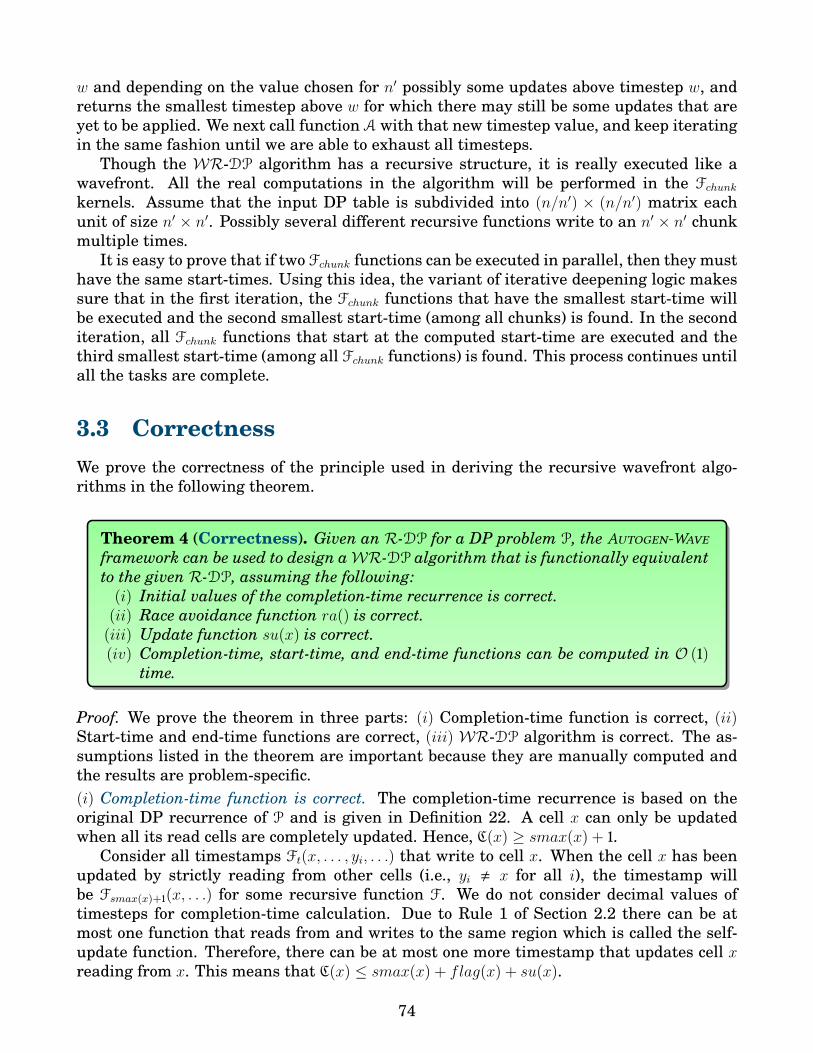
w and depending on the value chosen for n′ possibly some updates above timestep w, andreturns the smallest timestep above w for which there may still be some updates that areyet to be applied. We next call function A with that new timestep value, and keep iteratingin the same fashion until we are able to exhaust all timesteps.

Though the WR-DP algorithm has a recursive structure, it is really executed like awavefront. All the real computations in the algorithm will be performed in the Fchunkkernels. Assume that the input DP table is subdivided into (n/n′) × (n/n′) matrix eachunit of size n′ × n′. Possibly several different recursive functions write to an n′ × n′ chunkmultiple times.

It is easy to prove that if two Fchunk functions can be executed in parallel, then they musthave the same start-times. Using this idea, the variant of iterative deepening logic makessure that in the first iteration, the Fchunk functions that have the smallest start-time willbe executed and the second smallest start-time (among all chunks) is found. In the seconditeration, all Fchunk functions that start at the computed start-time are executed and thethird smallest start-time (among all Fchunk functions) is found. This process continues untilall the tasks are complete.

3.3 CorrectnessWe prove the correctness of the principle used in deriving the recursive wavefront algo-rithms in the following theorem.

Theorem 4 (Correctness). Given an R-DP for a DP problem P, the Autogen-Wave

framework can be used to design aWR-DP algorithm that is functionally equivalentto the given R-DP, assuming the following:

(i) Initial values of the completion-time recurrence is correct.(ii) Race avoidance function ra() is correct.

(iii) Update function su(x) is correct.(iv) Completion-time, start-time, and end-time functions can be computed in O (1)

time.

Proof. We prove the theorem in three parts: (i) Completion-time function is correct, (ii)Start-time and end-time functions are correct, (iii) WR-DP algorithm is correct. The as-sumptions listed in the theorem are important because they are manually computed andthe results are problem-specific.(i) Completion-time function is correct. The completion-time recurrence is based on theoriginal DP recurrence of P and is given in Definition 22. A cell x can only be updatedwhen all its read cells are completely updated. Hence, C(x) ≥ smax(x) + 1.

Consider all timestamps Ft(x, . . . , yi, . . .) that write to cell x. When the cell x has beenupdated by strictly reading from other cells (i.e., yi , x for all i), the timestamp willbe Fsmax(x)+1(x, . . .) for some recursive function F. We do not consider decimal values oftimesteps for completion-time calculation. Due to Rule 1 of Section 2.2 there can be atmost one function that reads from and writes to the same region which is called the self-update function. Therefore, there can be at most one more timestamp that updates cell xreading from x. This means that C(x) ≤ smax(x) + flag(x) + su(x).

74

Thus, C(x) = smax(x) + flag(x) + su(x) is correct.(ii) Start-time and end-time functions are correct. We prove the correctness of start-timefunctions. Similar arguments hold for end-time functions.

Start-time recurrences are given in Definition 23. A recursive function F(X, Y1, . . . , Ys)invokes O (1) number of child functions F′(X ′, Y ′1 , . . . , Y ′s ) such that X ′ and Y ′i are d-D or-thants of X and Yi, respectively. The start-time of F must be the minimum among childfunctions F′ of F. Hence, the recurrence case that SF (X, . . . , Yi, . . .) = minSF′ (X ′, . . . , Y ′i , . . .)is correct.

To compute the base cases of the start-time recurrence, we need to analyze two cases:(i) F is an inflexible function i.e., x ∈ y1, . . . , ys, and (ii) F is a flexible function i.e., x <y1, . . . , ys.

In the first case, the start-time of the inflexible function is same as the completion-time of the write-cell, because inflexible function represents complete updates. In the sec-ond case, the flexible function F(x, y1, . . . , ys) can immediately start once all the read cellsy1, . . . , ys have been updated completely i.e., SF (x, y1, . . . , ys) = max1≤i≤sC(yi) + 1. To avoidrace conditions, we add manually computed race avoidance condition ra(x, y1, . . . , ys). Thus,the start-time function (resp. end-time function) is correct.(iii) Recursive divide-and-conquer wavefront algorithm is correct. For all possible recursivefunctions F and regions X, Y1, . . . , Ys such that each region has a dimension length of n′, letw0 < w1 < · · · < wL−1 be all the start-times of F(X, Y1, . . . , Ys). As per the fundamental defini-tion of a wavefront algorithm, initially, all those chunks X for which SF (X, Y1, . . . , Ys) = w0will be executed. Then, chunks for which the start-times are w1 will be executed. Thisprocess continues till wL−1. We need to prove the recursive wavefront algorithm too followsthis strategy.

Once the timing functions are found, we simply plug in the start-time and end-timefunctions for every single recursive function call, as shown in an example in Figure 3.1, insuch a way that every recursive function is invoked at its start-time and finishes at its end-time and this is true assuming that the timing functions are correct. Using contradictionit is straightforward to prove that a function cannot start (resp. end) execution before orlater than its start-time (resp. end-time). It is up to the scheduler to schedule the recursivefunctions based on the timing functions.

The generic scheduling method to schedule a hybrid recursive wavefront algorithm usesa variant of iterative deepening technique to execute the base case tasks in a wavefrontmanner satisfying the DP dependencies and retaining the recursive structure, as depictedin an example in Figure 3.1. The scheduler (or programmer) adds conditional checks be-fore every invocation of a recursive function call to check whether the executing wavefrontlevels are in fact between the start-time and end-time of the function. If they are, then thecorresponding function is invoked to execute. As we do not execute a recursive functionbefore its start-time or after its end-time, we are not violating any original DP dependen-cies.

3.4 Scheduling algorithmsIn this section, we show how to schedule recursive wavefront algorithms to achieve prov-ably good bounds (optimal or near-optimal) for both parallelism and cache performance.

75

Recall that our recursive wavefront algorithm switches to the original non-wavefrontrecursive algorithm when the input parameter n drops to a value ≤ n′. While both recur-sive (wavefront and non-wavefront) algorithms have the same serial work complexity T1and same serial cache complexity Q1 (as they reduce to the same serial algorithm), theirspans are different. We use TR∞(n′) to denote the span of the non-wavefront algorithm for aproblem of size n′.

In this section, we present a provably efficient method of scheduling recursive wavefrontalgorithms on a parallel machine based on iterative deepening. We analyze the schedulingof the recursive wavefront algorithms using two schedulers: (a) work-stealing scheduler,and (b) a variant of the space-bounded scheduler.

A scheduler maps parallel tasks of a multithreaded program to different processors ina parallel machine. Several schedulers have been proposed, analyzed, and implemented inliterature. Table 3.6 gives a summary of several schedulers. Optimal algorithms scheduledusing bad schedulers does not lead to high-performance and similarly slow algorithmsscheduled using the best schedulers also do not lead to great performance. For the bestperformance, we need parallel algorithms with good cache efficiency and good parallelismand also scheduling algorithms (or schedulers) that exploit these characteristics.

It is not clear how to develop truly efficient cache-oblivious algorithms that have bothoptimal parallel cache performance and optimal parallelism. Even if we have high-performingalgorithms, developing a scheduler that exploits the best from the two worlds is non-trivial.The fundamental difficulty for solving the two problems above comes from two seeminglyparadoxical reasons:

(i) to get optimal parallel cache efficiency (majorly due to temporal locality), a taskshould work on a localized data as much as possible and migration of tasks to dif-ferent caches should be minimized.

(ii) to get optimal parallelism or at least good parallelism, the task migration should beencouraged because more migration means more parallelism.

We prove that the span of the pure recursive wavefront algorithms is at most linear(w.r.t the input parameter) in Lemma 1. We use the notations TR∞(n) and TW∞ (n) to de-note the span of recursive and recursive wavefront algorithms, respectively. Consider arecursive wavefront algorithm that switches to recursive kernels when the input param-eter drops from n to less than or equal to n′. Such algorithms are called hybrid recursivewavefront algorithms and in Sections 3.4.1 and 3.4.2 complexities of those algorithms whenscheduled using different schedulers are discussed.

Lemma 1 (Worst-case linear span of the recursive wavefront algorithms(without scheduling overhead)). Given a DP problem, if the completion-time(see Definition 22) of every cell (i1, . . . , im) can be written in the form

C(i1, . . . , im)← C(i1 − i′1, . . . , im − i′m) +O (1) (3.13)

where m is a constant; i1, . . . , im, i′1, . . . , i′m ∈ [0, n− 1] and at least one among i′1, . . . , i′mis greater than or equal to 1. Then the number of wavefront levels in the recursivewavefront algorithm is at most linear, i.e., NW

∞ (n) = O (n).

Proof. Let n denote the input parameter. Let a cell to be computed be represented usingm-dimensions (m is fixed). Let the cells (0, . . . , 0), (n − 1, . . . , n − 1)), (i1, . . . , im), and (i1 −

76

i′1, . . . , im − i′m) be denoted by first, last, x, and y, respectively. Let y be the cell such thatC(y) = rmax(x). Here, i1, . . . , im, i′1, . . . , i′m ∈ [0, n − 1] and at least one among i′1, . . . , i

′m is

greater than or equal to 1. Without loss of generality, we assume that first and last cellsare the initial and final cells to be fully updated, respectively and the cell x depends ony. We know that C(x) is more than C(y) by some non-negative constant. We need to provethat the number of wavefront levels in the algorithm is at most linear i.e., C(last) is O (n).

Given that the cell x depends on y, it is easy to see there is difference in the coordinatesof x and y in at least one dimension and the index of that dimension decreases from cell xto cell y by at least 1. The maximum number of times the reduction in index in a singledimension can happen is n. As there are m dimensions, in the worst case, the maximumnumber of times reduction in any dimension can occur is nm. In other words, startingfrom final, it takes nm = O (n) time steps to reach first cell and in each timestep thereis a difference of a constant value in the completion times of the write and the read cells.Therefore, C(last) is O (n) and hence NW

∞ (n) = O (n).

3.4.1 Work-stealing scheduler

In this section, we analyze the complexity of the hybrid recursive wavefront algorithmswhen scheduled using a randomized work-stealing (WS) scheduler [Blumofe and Leiserson,1999].

The machine model for WS is a machine with several levels of distributed privatecaches. The randomized WS presented and analyzed in [Blumofe and Leiserson, 1999] isa distributed cache-oblivious scheduler that can schedule hybrid recursive wavefront algo-rithms to get good parallel cache performance and good parallelism. We prove the followingtheorem to analyze the complexities of the schedule.

Scheduler Qp Tp CommentsGreedy scheduler − O

(T1p

+ T∞)

Random work-stealing O(Q1 + pM

BT∞

)O(T1p

+ T∞)

Non-optimal Qp

Priority work-stealing O(Q1 + pM

BT∞

)O(T1p

+ T∞)

Non-optimal Qp

Parallel depth-first Ω (Q1) O(T1p

+ T∞)

Mp = Ω (M1 + Θ (pT∞))Space-bounded O (Q1) O

(T1p

+ T∞)

Non-optimal T∞W-SB O (Q1) O

(T1p

+ T∞)

Optimal Qp and near-optimal T∞

Table 3.6: Parallel cache complexity (Qp) and parallel running time (Tp) of several sched-ulers.

77

Theorem 5 (WS complexity). Suppose a DP recurrence is evaluated by the WI-DP in N∞(n) parallel steps with ∞ processors. When the WR-DP algorithm withswitching point n′ ≤ n (switching to n R-DP) evaluates the recurrence, we achievethe following bounds while using a randomized work-stealing (WS) scheduler:

O work, T1(n) = O(TR1 (n)

),

O span, T∞(n) = O(N∞( n

n′)(O (log n) + TR∞(n′)

)),

O parallel time, Tp(n) = O(T1(n)p

+ T∞(n))

w.h.p. in n,O serial cache complexity, Q1(n) = T1(n/n′)QR

1 (n′),O parallel cache complexity, Qp(n) = O

(Q1(n) + p · M

B· T∞(n)

)w.h.p. in n, and

O extra space, Sp(n) = O (p log n).We assume that N∞(n) and T1(n) (work) are polynomials of n, and choose n′ such

that T1(n′) = Ω (log n).

Proof. The theorem is proved in different parts.Span. The total span is found by summing up the spans at every wavefront level. Thespan is bounded using a simple formula: total span ≤ #(wavefront levels) × (worst-casespan of executing a chunk + worst-case span to reach a chunk). We know that thereare N∞(n/n′) wavefront levels in the algorithm as the outer loop (e.g., the loop insideRECURSIVE-WAVEFRONT-PARENTHESIS of Figure 3.1) in the recursive wavefront algo-rithm will iterate N∞(n/n′) times. The worst-case span of executing a chunk is TR∞(n′).Also, the worst-case span to reach a chunk is O (log(n/n′)). Simplifying, we have the totalspan as N∞(n/n′)(O (log n) + TR∞(n′)).Total work. Similar to span, the total work can be found by summing up the work done atevery wavefront level. The total work can be bounded using a simple formula: total work= #(chunks) ×(#computations inside a chunk + #computations required to reach a chunk).The expression computes to T1(n/n′) (T1(n′) +O (log(n/n′))). We assume that the work is apolynomial function of n, which implies T1(n/n′) = T1(n)/T1(n′). To not increase the workcompared to the original wavefront algorithm, we assume that every chunk does Ω (log n)work, which implies T1(n′) + Θ (log n) = T1(n′). After substitutions and simplification, thetotal work remains Θ (T1(n)) and does not increase.Parallel running time. The parallel running time at a specific wavefront level is foundusing the theorem from [Blumofe and Leiserson, 1999]. The parallel running time Tp(n) ofthe entire algorithm is found by summing up the parallel running time at each wavefrontlevel. Let T (i)

1 , T (i)∞ and Q

(i)1 be the work, span and serial cache complexity, respectively, of

the ith iteration of the outer loop in the recursive wavefront algorithm. Then the parallelrunning time of that iteration under the WS scheduler is O

(1 + T

(i)1 (n)/p+ T (i)

∞ (n))

(w.h.p.).We sum up over all i, and obtain the claimed bound for Tp(n). Thus, we have

Tp(n) = O ∑

level i

(1 + work at iteration i

p+ span at iteration i

)= O

#(wavefront levels) + 1p·∑

level iT

(i)1 (n) +

∑level i

T (i)∞ (n)

= O

(#(wavefront levels) + 1

p· T1(n) + T∞(n)

)= O

(T1(n)p

+ T∞(n))

78

Serial cache complexity. The total serial cache complexity can be found using the for-mula: Q1(n) = #(chunks) × (serial cache complexity of a chunk + serial cache complex-ity of reaching a chunk) = T1(n/n′)

(QR

1 (n′) + Θ ((log n)/B)). As T1(n′) = Ω (log n), we have

QR1 (n′) = Ω ((log n)/B) and on simplification we get Q1(n) = T1(n/n′)QR

1 (n′).Parallel cache complexity. The parallel cache complexity at a particular level is found by aresult from [Acar et al., 2000] in terms of serial cache complexity. Similar to the argumentof parallel running time, the total parallel cache complexity Qp(n) comprises of the parallelcache complexity at all levels. The parallel cache complexity of the i-th iteration of theouter loop is O

(Q

(i)1 (n) + p(M/B)T (i)

∞ (n))

(w.h.p.) under the WS scheduler. Summing upover all i gives us the claimed bound for Qp(n). We have

Qp(n) = O ∑

level i

(Q

(i)1 (n) + p · M

B· T (i)∞ (n)

)= O (Q1(n) + p(M/B) · T∞(n))

To achieve Qp(n) as described above w.h.p. we set ε = 1/n2+λ for any λ > 0 in Lemma 16of [Acar et al., 2000].Extra-space complexity. For p processors, there can be at most p tasks running in parallel.When the tasks reach the levels of the leaves of the recursion tree, they execute the logicin the leaf functions. As each executing task is a leaf node in the recursion tree, we mightrequire a total extra space all along the path from the root to the p executing leaves of therecursion tree. Hence, Sp(n) = O (p log n).

If n′ is a polynomial function of n with degree less than 1 and Lemma 1 is satisfied, thenwe have the following corollary derived from Theorem 5.

Corollary 1 (WS complexity). In the hybrid recursive wavefront algorithm, ifn′ = nα for some constant α ∈ [0, 1) and if Lemma 1 is satisfied, then WSschedules the algorithm on distributed cache machine to have Sp = O (p log n),T∞(n) = O

(n1−αTR∞(nα)

), Q1(n) = T1(n1−α)QR

1 (nα), Tp(n) = O (T1(n)/p+ T∞(n)), andQp(n) = Θ (Q1(n) + p(M/B)T∞(n)) and the latter two bounds are satisfied w.h.p. Forthe Tp(n) and Qp(n) equations to hold, we assume that T1(n) is a polynomial of n, andchoose n′ such that T1(n′) = Ω (log n).

3.4.2 Modified space-bounded schedulerIn this section, we show how to modify a space-bounded scheduler(W-SB) [Chowdhuryet al., 2013] so that it can execute a recursive wavefront algorithm cache-optimally withnear-optimal parallelism.

The parallel memory hierarchy (PMH) [Blelloch et al., 2011] model models the memoryhierarchy of many real parallel systems. It is described in Section 1.4.2 and we use thismemory model for the scheduler. The W-SB scheduler combines two ideas: timing functionspresented in Section 3.2 and space-bounded scheduler introduced in [Chowdhury et al.,2010,Chowdhury et al., 2013].

79

For each recursive function call, our W-SB scheduler accepts three hints: start-time,end-time and working set size (i.e., total size of all regions in the DP table accessed bythe function call). Given an implementation of a standard recursive algorithm with eachfunction call annotated with those three hints, the W-SB can automatically generate a re-cursive wavefront implementation (similar to the one on the right hand side of Figure 3.1).From the given start-times, the scheduler determines the lowest start-time and executesthe tasks that can be executed at that lowest start-time. Since the scheduler knows all thecache sizes, as soon as the working set size of any function executing on a processor undera cache fits into that cache, the scheduler anchors the function to that cache in the sensethat all recursive function calls made by that function and its descendants will only be ex-ecuted by the processors under that anchored cache. This approach of limiting migrationof tasks ensures cache-optimality [Chowdhury et al., 2013,Blelloch et al., 2011].

The W-SB scheduler is centralized and cache-aware. It schedules recursive wavefrontalgorithms in which the number of recursive function calls made by a function is upperbounded by a constant. The complete information related to a function call is given byby T = [SF (X, Y1, . . . , Ys) , EF (X, Y1, . . . , Ys)] : F(X, Y1, . . . , Ys). That is, this scheduler acceptsstart-time, end-time and problems size for each function call. From the given start-times,the scheduler determines the lowest start-time and executes the tasks that can be executedat that lowest start-time. If there are p processors in the machine, then at any point in timea maximum of p tasks can be executed in parallel. The subtask T of a task T′ is said to beanchored to a cache at some level if T fits into the cache but not T′. When a task T isanchored to a cache M, the task and all of its subtasks at all granularities will be in thesame cache and they will not be migrated to any other cache that is not part of the subtreeof caches rooted at M. A similar argument holds for all cache levels and hence when a taskfits into a cache as much useful work is done as possible.

A task is a subproblem that writes to a region of an input DP table and reads from one ormore regions. The complete information related to a task is denoted by T = [SF (X, Y1, . . . , Ys) ,EF (X, Y1, . . . , Ys)] : F(X, Y1, . . . , Ys). That is, this scheduler accepts start-time, end-time andproblems size for each function call/task. From the given start-times, the scheduler de-termines the lowest start-time and executes the tasks that can be executed at that loweststart-time. If there are p processors in the machine, then at any point in time a maximumof p tasks can be executed in parallel. The subtask T of a task T′ is said to be anchoredto a cache at some level if T fits into the cache but not T′. When a task T is anchored to acache M, the task and all of its subtasks at all granularities will be in the same cache andthey will not be migrated to any other cache that is not part of the subtree of caches rootedat M. A similar argument holds for all cache levels and hence when a task fits into a cacheas much useful work is done as possible.

Example. For simplicity of exposition, we describe here the process by which W-SB sched-ules a recursive wavefront algorithm for the LCS problem on a 16 × 16 DP table X witha chunk size of 4 × 4 after which it switches to standard 2-way recursive algorithm. Inthe PMH model, we assume h = 2, f2 = 2, f1 = 1, and M1 has just enough memory toexecute 4 × 4 subproblem. As per the scheduling method shown in Figure 3.1, the basecase size n′ will be chosen by the scheduler automatically such that it is equal to M1 asLCS can be implemented in linear space. In the first iteration the wavefront level is 0 andthe only task that would be executed is [0, 6] : A(X11,11). As this task fits in M1, it will beexecuted completely before it is knocked off from the cache. During the execution of first

80

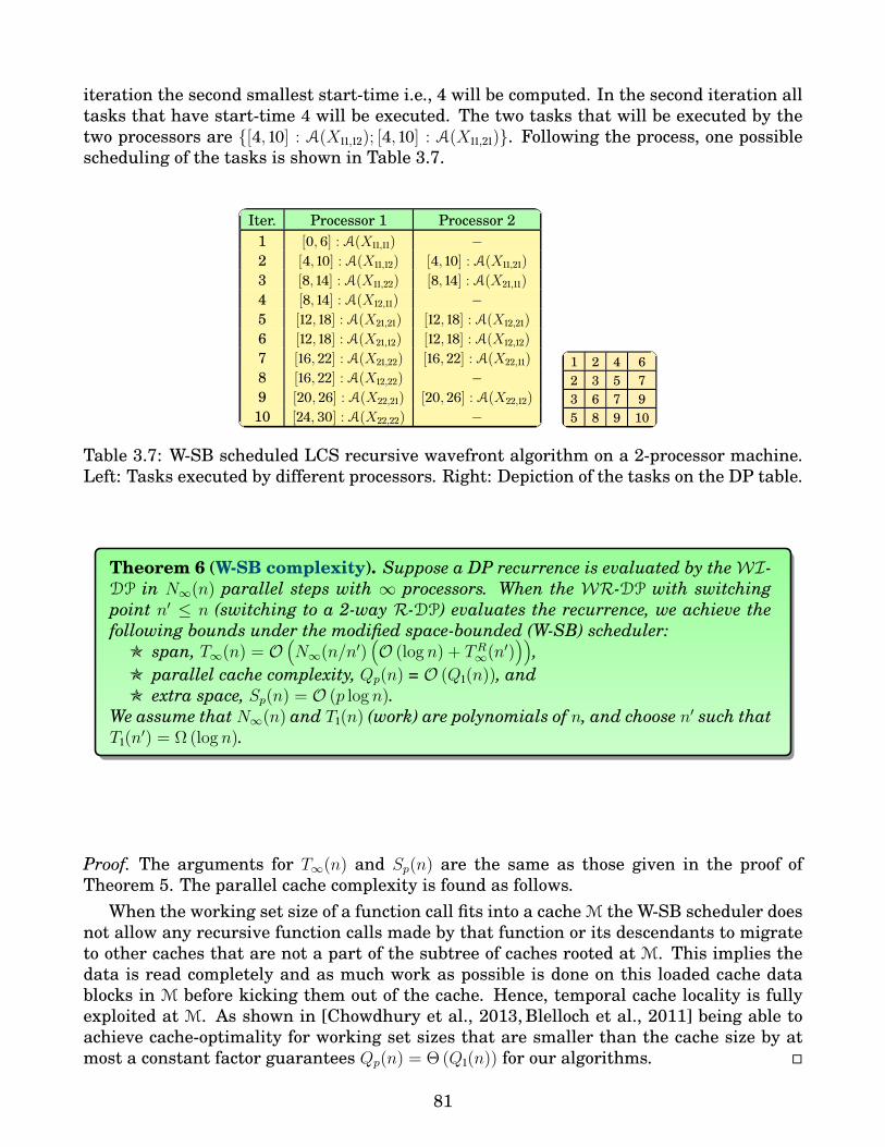
iteration the second smallest start-time i.e., 4 will be computed. In the second iteration alltasks that have start-time 4 will be executed. The two tasks that will be executed by thetwo processors are [4, 10] : A(X11,12); [4, 10] : A(X11,21). Following the process, one possiblescheduling of the tasks is shown in Table 3.7.

Iter. Processor 1 Processor 21 [0, 6] : A(X11,11) −2 [4, 10] : A(X11,12) [4, 10] : A(X11,21)3 [8, 14] : A(X11,22) [8, 14] : A(X21,11)4 [8, 14] : A(X12,11) −5 [12, 18] : A(X21,21) [12, 18] : A(X12,21)6 [12, 18] : A(X21,12) [12, 18] : A(X12,12)7 [16, 22] : A(X21,22) [16, 22] : A(X22,11)8 [16, 22] : A(X12,22) −9 [20, 26] : A(X22,21) [20, 26] : A(X22,12)

10 [24, 30] : A(X22,22) −

1 2 4 62 3 5 73 6 7 95 8 9 10

Table 3.7: W-SB scheduled LCS recursive wavefront algorithm on a 2-processor machine.Left: Tasks executed by different processors. Right: Depiction of the tasks on the DP table.

Theorem 6 (W-SB complexity). Suppose a DP recurrence is evaluated by theWI-DP in N∞(n) parallel steps with ∞ processors. When the WR-DP with switchingpoint n′ ≤ n (switching to a 2-way R-DP) evaluates the recurrence, we achieve thefollowing bounds under the modified space-bounded (W-SB) scheduler:

O span, T∞(n) = O(N∞(n/n′)

(O (log n) + TR∞(n′)

)),

O parallel cache complexity, Qp(n) = O (Q1(n)), andO extra space, Sp(n) = O (p log n).

We assume that N∞(n) and T1(n) (work) are polynomials of n, and choose n′ such thatT1(n′) = Ω (log n).

Proof. The arguments for T∞(n) and Sp(n) are the same as those given in the proof ofTheorem 5. The parallel cache complexity is found as follows.

When the working set size of a function call fits into a cache M the W-SB scheduler doesnot allow any recursive function calls made by that function or its descendants to migrateto other caches that are not a part of the subtree of caches rooted at M. This implies thedata is read completely and as much work as possible is done on this loaded cache datablocks in M before kicking them out of the cache. Hence, temporal cache locality is fullyexploited at M. As shown in [Chowdhury et al., 2013, Blelloch et al., 2011] being able toachieve cache-optimality for working set sizes that are smaller than the cache size by atmost a constant factor guarantees Qp(n) = Θ (Q1(n)) for our algorithms.

81

Corollary 2 (W-SB complexity). If Lemma 1 is satisfied, if Θ(nd)

is the size of theinput DP table, then the W-SB scheduler schedules the hybrid recursive algorithmalgorithm on a PMH machine model to achieve the following bounds:

O If n′ = nα for some constant α ∈ [0, 1), then T∞(n) = O(n1−αTR∞(nα)

).

O If n′ = Θ(M 1/d

), where M is a cache-size, then T∞(n) =

O((n/M 1/d)(log n+ TR∞(M 1/d))

).

In both the cases, we have Qp(n) = Θ (Q1(n)) and Sp(n) = O (p log n) or Sp(n) =O (pS1(n)).

3.5 Further improvement of parallelismWe develop algorithms to asymptotically improve the parallelism of the divide-and-conquerwavefront (WR-DP) algorithms. We explain the algorithm in simple words (without pseu-docode) and then analyze it for its complexities.

The new algorithm works as follows. We set the switching point as n′ = f(n) wheref(n) = o (n). The standard WR-DP algorithms switches to an R-DP chunk when theproblem parameter n reduces to less than or equal to n′. In the new algorithm, when theproblem parameter n reduces to less than or equal to f(n), instead of calling the R-DP

algorithm we call the same divide-and-conquer wavefront algorithm. Now the divide-and-conquer wavefront algorithm works on a subproblem with subproblem parameter f(n) andswitches the algorithm when the subprobem parameter reduces to less than or equal tof(f(n)). This process continues recursively.

Complexity analysis. Let T∞(n, f(n)) denote the span of this new algorithm. Let T∞(n)denote the span of the pureWR-DP algorithm with switch-point n′ = 1. Then,

T∞(n, f(n)) =

Θ (1) if n = 1,Θ(

nf(n)

)· (T∞ (f(n), f(f(n))) +O (log n) + Θ (1)) if n > 1.

Let T1(n, f(n)) denote the work of this new algorithm. Let T1(n) denote the work of thepureWR-DP algorithm with switch-point n′ = 1. Then,

T1(n, f(n)) =

Θ (1) if n = 1,T1

(n

f(n)

)· (T1 (f(n), f(f(n))) +O (log n) + Θ (1)) if n > 1.

When f(n) = log n, we have

T∞(n, log n) ≤ c

(n

log n

)· (T∞ (log n, log log n) + c′ log n)

≤ c

(n

log n

)(c

(log n

log log n

)· (T∞ (log log n, log log log n) + c′ log log n) + c′ log n

)

= c2(

n

log log n

)· T∞ (log log n, log log log n) + cc′ (c+ 1)n

= clog∗ n · n+ cc′(c(log∗ n)−1 + c(log∗ n)−2 + · · ·+ 1

)n ≤ clog∗ n · n+ c(log∗ n)+1c′n

= Θ(clog∗ n · n

)

82

It is easy to see that this span is asymptotically better (or smaller) than Θ (n log n) asΘ(clog∗ n

)= o (log n).

Let Li(n) = log log · · · log n Assuming T1(n) is a polynomial function of n, the total workT1(n, log n) can be computed as

T1(n, log n) = T1

(n

log n

)(T1 (log n, log log n) + c log n)

= T1

(n

log n

)· T1 (log n, log log n) + cT1

(n

log n

)· log n

= T1

(n

log n

)· T1

(log n

log log n

)· (T1 (log log n, log log log n) + c log log n) + cT1

(n

log n

)· log n

= T1

(n

log n

)· T1

(log n

log log n

)· T1 (log log n, log log log n)

+ cT1

(n

log log n

)· log log n+ cT1

(n

log n

)· log n

= T1

(n

log n

)· T1

(log n

log log n

)· · ·Θ (1) + c′T1(n)

= T1(n)T1(log n) ·

T1(log n)T1(log log n) · · ·Θ (1) + c′T1(n)

= Θ (T1(n))

3.6 Experimental resultsIn this section we present experimental results showing performance of recursive wave-front algorithms for the parenthesis and the 2D FW-APSP problems. We also compareperformance of those algorithms with the corresponding standard 2-way recursive divide-and-conquer and the original cache-oblivious wavefront (COW) algorithms [Tang et al.,2015]. The recursive wavefront algorithms were implemented by Jesmin Jahan Tithi.

We used C++ with Intel Cilk™ Plus extension to implement all algorithms presentedin this section. Therefore, all implementations basically used the work-stealing schedulerprovided by Cilk™ runtime system. All programs were compiled with -O3 -ip -parallel

-AVX -xhost optimization parameters. To measure cache performance we used PAPI-5.3[PAP, ]. Table 3.8 lists the systems on which we ran our experiments.

3.6.1 Projected parallelismSince we still do not have shared-memory multi-core machines with thousands of cores,we have used the Intel Cilkview scalability analyzer to compute the ideal parallelism andburdened span of the following implementations:

(i) recursive wavefront algorithm that does not switch to the 2-way non-wavefront recur-sive algorithm and instead directly uses an iterative basecase (wave),

(ii) recursive wavefront algorithm that switches to the 2-way recursive divide-and-conquerat some point (wave-hybrid),

(iii) standard 2-way recursive divide-and-conquer algorithm (CO_2Way).

83

Model E5-2680 E5-4650 E5-2680Cluster Stampede [Sta, ] Stampede [Sta, ] Comet [Com, ]#Cores 2x8 4x8 2x12Frequency 2.70GHz 2.70GHz 2.50GHzL1 32K 32K 32KL2 256K 256K 256KL3 20480K 20480K 30720KCache-line size 64B 64B 64BMemory 64GB 1TB 64GBCompiler 15.0.2 15.0.2 15.2.164OS CentOS 6.6 CentOS 6.6 CentOS 6.6

Table 3.8: System specifications.

124816326412825651210242048

1024 2048 4096 8192 16384

Parallelism

n

Parenthesis - Parallelism

CO_2way Wave Wave_hybrid

24816326412825651210242048

1024 2048 4096 8192 16384

Parallelism

n

FW-APSP - Parallelism

CO_2way Wave Wave_hybrid

Figure 3.2: Projected scalability of new recursive wavefront algorithms by Cilkview Scal-ability Analyzer. The numbers basically denote till how many cores the implementationshould scale linearly.

For wave-hybrid, we have used n′ = max256, power of 2 closest to n2/3. In order to re-duce overhead of recursion and to take advantage of vectorization we switch to an iterativekernel when n becomes sufficiently small (e.g., 64 for wave, wave-hybrid and CO_2Way).

Figure 3.2 shows the scalability results reported by Cilkview for algorithms solving theparenthesis problem and Floyd-Warshall’s APSP. These parallelism numbers show thatrecursive wavefront algorithms scale much better than standard 2-way recursive divide-and-conquer algorithms.

3.6.2 Running time and cache performanceFigure 3.3 shows performance of the following on a 16-core Sandy Bridge machine: (i)wave, (ii) wave-hybrid, (iii) CO_2Way, and (iv) our original cache-oblivious wavefront (COW)algorithms with atomic locks from [Tang et al., 2015]. For wave-hybrid, we have usedn′ = max256, power of 2 closest to n2/3. In order to reduce overhead of recursion andto take advantage of vectorization we switch to an iterative kernel when n becomes suf-ficiently small (e.g., 64 for wave, wave-hybrid and CO_2Way). It is clear from the figuresthat wave and wave-hybrid algorithms perform better than CO_2Way and the COW algo-rithms for all cases. For parenthesis problem, wave is 2.6×, and wave-hybrid is 2× faster

84

than CO_2Way. Similarly, number of cache misses of CO_2Way is slightly higher than thatof both wave and wave-hybrid. For Floyd-Warshall’s APSP, wave is 18%, and wave-hybrid

is 10% faster than CO_2Way. Therefore, even with 16 cores, the impact of improvements inparallelism and cache-misses is visible on the running time. On the other hand, thoughCOW algorithms have excellent theoretical parallelism, their implementations heavily useatomic locks, which may have impacted their performance negatively for large n and forDP dimension d > 1.

Figure 3.3: Runtime and cache misses in three levels of caches for classic 2-way recur-sive divide-and-conquer, COW and recursive wavefront algorithms for Parenthesis and 2DFW-APSP Problems. All programs were run on 16 core machines in Stampede. All imple-mentations used Cilk Plus’s work-stealing scheduler.

We have obtained performance results on a 24-core Haswell machine (shown in Figure3.4). Value of n′ and size of iterative kernel were determined in the same way as we didon Stampede. For FW-APSP, wave is 15% and wave-hybrid is 10% faster than CO_2Way. Al-though we see improvement in L1 and L2 cache misses, number of L3 misses is worseprobably due to the increased parallelism. For parenthesis problem, wave is 16% andwave-hybrid is 18% faster than CO_2Way, and we see only improvement in the L3 cachemisses.

On a 32-core Sandy Bridge machine, wave for FW-APSP runs 73% faster and wave-hybrid

runs 69% faster than CO_2Way. On the other hand, for the parenthesis problem both wave

and wave-hybrid are 2.1× faster than CO_2Way.

3.7 Conclusion and open problemsIn this chapter we presented a framework to semi-automatically discover divide-and-conqueralgorithms that achieve extremely high parallelism retaining excellent cache-efficiency

85

Figure 3.4: Runtime and cache misses in three levels of caches for classic 2-way recur-sive divide-and-conquer, COW and recursive wavefront algorithms for Parenthesis and 2DFW-APSP Problems. All programs were run on 24 core machines in Comet. All implemen-tations used cilk plus’s work-stealing scheduler.

(i.e., temporal locality). The presented WR-DP algorithms are theoretically fastest dy-namic programming implementations.

Some open problems that could be investigated are as follows:O [Full automation.] Completely automate the discovery of WR-DP algorithms (then

the Autogen-Wave framework will be transformed to Autogen-Wave algorithm) in-cluding computing completion-time functions and computing ra() – race avoidancecondition.

O [Improve span to Θ (n).] TheWR-DP algorithms have the best-case span of Θ (n log n).Is it possible to improve this best-case span to Θ (n)?

O [WR-DP algorithms for matrix problems.] Design WR-DP algorithms for severalnon-DP matrix problems (e.g.: QR decomposition, SVD decomposition, etc). A verygood source of matrix algorithms is [Golub and Van Loan, 2012].

86

Chapter 4

An Efficient Divide-&-Conquer ViterbiAlgorithm

The Viterbi algorithm is used to find the most likely path through a hidden Markov modelgiven an observed sequence, and has numerous applications. Due to its importance andhigh computational complexity, several algorithmic strategies have been developed to par-allelize it on different parallel architectures. However, none of the existing algorithms forthe Viterbi decoding problem is simultaneously cache-efficient and cache-oblivious. Be-ing oblivious of machine resources (e.g., caches and processors) while also being efficientpromotes portability.

In this chapter, we present an efficient cache- and processor-oblivious Viterbi algorithmbased on rank convergence solving the two decade old open problem. The algorithm buildsupon the parallel Viterbi algorithm of Maleki et al. (PPoPP 2014). We provide empiricalanalysis of our algorithm by comparing it with Maleki et al.’s algorithm. To the best of ourknowledge, this is the first work that presents a provably cache-efficient cache-obliviousparallel Viterbi algorithm.

4.1 IntroductionThe Viterbi algorithm [Viterbi, 1967,Viterbi, 1971,Forney Jr, 1973,Omura, 1969,Lou, 1995]which was proposed by Andrew J. Viterbi (co-founder of Qualcomm) in 1967 is a dynamicprogramming algorithm that finds the most probable sequence of hidden states from agiven sequence of observed events. As each observation is a probabilistic function of a hid-den state, the discrete-time finite-state Markov process is modeled using a hidden Markovmodel (HMM). An excellent tutorial on HMM can be found in [Rabiner, 1989].

The Viterbi algorithm has numerous real world applications. Viterbi developed his al-gorithm as a decoding method for convolutional codes in noisy communication channels.Since then, the algorithm has found wide applications in Qualcomm’s CDMA technol-ogy [Gilhousen et al., 1991, Kand and Willson, 1998, Feldman et al., 2002], TDMA sys-tem for GSM [Costello et al., 1998], television sets [Nam and Kwak, 1998], satellite andspace communication [Heller and Jacobs, 1971], speech recognition [Rabiner, 1989, Soongand Huang, 1991,Franzini et al., 1990], handwritten word recognition [Kundu et al., 1988],hand gesture recognition [Chen et al., 2003], modems [Ungerboeck, 1982], magnetic record-ing systems [Kobayashi, 1971a, Kobayashi, 1971b], biological sequence analysis [Hender-

87

son et al., 1997, Durbin et al., 1998], parsing context-free grammars [Klein and Manning,2003, Schmid, 2004], and part-of-speech tagging [Cutting et al., 1992, Taylor and Black,1998]. In 2006, Forney [Forney Jr, 2005] asserted that the Viterbi decoder was being usedin about a billion cellphones and that approximately 1015 bits of data were being decodedby the Viterbi algorithm in the digital television sets per second. Due to the immense sig-nificance of the algorithm and other contributions, Viterbi received the National Medal ofTechnology (US) in 2007 and the National Medal of Science (US) in 2008.

The 214-state big Viterbi decoder (BVD) [Collins, 1992] built by Jet Propulsion Labo-ratory (JPL) in 1992 for Galileo space mission is the largest Viterbi decoder in use. Itis important to develop fast parallel Viterbi algorithms for gigantic number of states andtimesteps for multicore and many core machines. When the input data of an algorithmis too large to fit into a cache, the time spent by the algorithm in block transfers (or IO)between adjacent levels of caches becomes more significant than the time taken for theCPU computations. In such cases, a cache-efficient Viterbi algorithm that minimizes thenumber of cache misses is desired. Though there have been a lot of efforts and successesin parallelizing the Viterbi algorithm, there is little work in the realm of designing cache-efficient algorithms for the Viterbi problem. To the best of our knowledge, we present thefirst cache-efficient Viterbi algorithm.

An algorithm that can be easily ported to different computing platforms from cellphonesto supercomputers should be cache-oblivious [Frigo et al., 1999] and processor-oblivious. Acache-oblivious algorithm need not know the cache parameters such as cache size and blocksize. Similarly, a processor-oblivious algorithm need not know the number of processors onthe machine it runs on. Several cache- and processor-oblivious algorithms for dynamicprograms that are majorly based on recursive divide-and-conquer have been developed,analyzed, and implemented in [Cherng and Ladner, 2005,Chowdhury and Ramachandran,2006, Chowdhury and Ramachandran, 2008, Chowdhury and Ramachandran, 2010, Tanet al., 2006,Bille and Stckel, 2012].

Our contributions. The major contributions of this chapter are summarized as follows:(1) We present an efficient cache- and processor-oblivious Viterbi algorithm based on

rank convergence.(2) We present an efficient cache- and processor-oblivious recursive divide-and-conquer

Viterbi algorithm for multiple instances of the problem.(3) We present experimental results comparing our algorithms with the existing fastest

Viterbi algorithms.

Organization of the chapter. In Section 4.2, we give a simple cache-inefficient Viterbi al-gorithm based on recursive divide-and-conquer. In Section 4.3, we present a cache-efficientViterbi algorithm for multiple instances of the problem. A parallel Viterbi algorithm basedon rank convergence is described in Section 4.4. In Section 4.5, a cache-efficient parallelViterbi algorithm based on rank convergence is presented. Finally we conclude.

4.2 Cache-inefficient Viterbi algorithmIn this section, we give a formal specification of the Viterbi algorithm, and describe a simplecache-inefficient Viterbi algorithm based on recursive divide-and-conquer.

88

Formal specificationThe Viterbi algorithm is described as follows. We are given an observation space O =o1, o2, . . . , om, state space S = s1, s2, . . . , sn, observations Y = y1, y2, . . . , yt, transitionmatrix A of size n × n, where A[i, j] is the transition probability of transiting from si to sj,emission matrix B of size n × m, where B[i, j] is the probability of observing oj at si, andinitial probability vector (or initial solution vector) I, where I[i] is the probability that xi =si. Let X = x1, x2, . . . , xt be a sequence of hidden states that generates Y = y1, y2, . . . , yt.Then the matrices P and P ′ of size n × t, where P [i, j] is the probability of the most likelypath of getting to state si at observation oj and P ′[i, j] stores the hidden state of the mostlikely path are computed as follows.

P [i, j] =I[i] ·B[i, y1] if j = 1,maxk∈[1,n](P [k, j − 1]× A[k, i]×B[i, yj]) if j > 1.

P ′[i, j] =

0 if j = 1,argmaxk∈[1,n](P [k, j − 1]× A[k, i]×B[i, yj]) if j > 1.

There are two phases in the Viterbi algorithm. In the first phase called forward phase,the matrices P and P ′ are computed. In the second phase called backward phase, thesequence of hidden states X is computed from P ′ by traversing from the tth timestep of P ′to its first timestep and recursively computing the argument max at each timestep. Thetime complexity of the algorithm implemented naively is Θ (n2t).

Quite often, the forward phase dominates the execution time. Hence, in this paper,we focus only on the forward phase of the algorithm, i.e., computing P and/or P ′. Also,for all our algorithms, we assume that the matrices P, P ′, A, and B are stored in eithercolumn-major order or z-Morton order.

Irregular data dependencyViterbi algorithm is a dynamic programming (DP) algorithm having irregular dependencyas shown in Figure 4.1. It means that the data dependency does not follow a particularpattern for all cells in the matrix. The irregular dependency is due to the memory accessB[i, yj] that depends on the value of yj, which in turn depends on a problem instance. Webelieve the Viterbi problem is the first DP problem with irregular dependency for which anefficient cache-oblivious algorithm is being presented.

The elements accessed in B changes depending on the value of yj. It is possible toconvert the problem with irregular data dependency to a problem with regular dependencyby transforming the matrix B of size n×m into another matrix C of size n×t. An algorithmto construct matrix C from matrix B is given in Figure 4.2.

Figure 4.1: Dependency structure of the Viterbi DP with irregular dependency: cell (i, j)depends on the green cells.

89

CONVERT-B-TO-C(B,C)

1. for j ← 1 to t do2. C[1 . . . n][j]← B[1 . . . n][yj ]

Figure 4.2: An algorithm to convert B matrix to C matrix.

After converting the B matrix to C, the Viterbi algorithm recurrence having regulardependency can be written as

P [i, j] =I[i]× C[i, 1] if j = 1,maxk∈[1,n](P [k, j − 1]× A[k, i]× C[i, j]) if j > 1. (4.1)

The new dependency structure is given in Figure 4.3. The serial cache complexity toconstruct C matrix is Θ (nt/B).

Cache-inefficient algorithmAn iterative parallel and a recursive divide-and-conquer-based parallel Viterbi algorithmsare given in Figure 4.4. The recursive divide-and-conquer algorithm was co-designed withVivek Pradhan. A visual depiction of the recursive algorithm is given in Figure 4.4. As perthe Viterbi recurrence, each cell (i, j) of matrix P depends on all cells of P at column j − 1,all cells of A at column i, and the cell (i, yj) of B. The function Avit fills jth column of Pdenoted by X using (j − 1)th column denoted by U using a divide-and-conquer approach.To compute each column of P , the entire matrix of A should be read. Hence the recursivealgorithm is cache-inefficient. In both algorithms, the cells in each stage (or timestep) arecomputed in parallel and the stages are computed sequentially.

Complexity analysis. The serial cache complexity of the iterative algorithm is computedas∑tj=1

∑ni=1O (n/B) = O (n2t/B) and that of the divide-and-conquer algorithm is computed

as follows. Let QA(n) denote the serial cache complexity of Avit on a matrix of size n × n.Then

QA(n) =O (n2/B + n) if n2 ≤ γAM ,4QA (n/2) +O (1) otherwise.

where, γA is a suitable constant. Solving, QA(n) = O (n2/B + n). Thus, the serial cachecomplexity of the recursive algorithm is O (n2t/B + nt) when n2 is too large to fit in cache.

Both the iterative and recursive algorithms have spatial locality, but they do not haveany temporal locality. Hence, these algorithms are not cache-efficient.

The span of the iterative algorithm is Θ (nt), as there are t time steps and it takes n timesteps to update a cell of P . The span of the recursive algorithm is computed as follows. Let

Figure 4.3: Dependency structure of the Viterbi DP with regular dependency: cell (i, j)depends on the green cells.

90

LOOP-VITERBI(P,A,B)

1. for j ← 2 to t do2. parallel for i← 1 to n do3. for k ← 1 to n do4. P [i, j]← max (P [i, j], P [k, j − 1]×A[k, i]×B[i, yj ])

VITERBI-D&C(P,A,B)

1. for j ← 2 to t do2. X ← P [.., j]; U ← P [.., j − 1]; V ← A; W ← B[.., yj ]3. Avit(X,U, V,W )

Avit(X,U, V,W )

1. if V is a small matrix then2. Aloop−vit(X,U, V,W )3. else4. parallel: Avit(X1, U1, V11,W1), Avit(X2, U1, V12,W2)5. parallel: Avit(X1, U2, V21,W1), Avit(X2, U2, V22,W2)

Figure 4.4: (a) Parallel iterative Viterbi algorithm and cache-inefficient parallel recursivedivide-and-conquer-based Viterbi algorithm. Note that we need not store the entire matrixP . We can keep a single column vector to compute the last column of matrix P . (b) Aparallel cache-inefficient recursive divide-and-conquer procedure for the Viterbi algorithm.The initial call to the function is Avit(X,U, V,W ). The first array is the array of matrix Pat column j, the second array is the (j − 1)th column of P , the third matrix is the matrix Aand the last array is the array of B at column yj. The algorithm updates the red regionsusing data from the blue regions.

TA(n) denote the span of Avit on a matrix of size n× n. Then

TA(n) = Θ (1) if n = 1,

2TA (n/2) + Θ (1) otherwise.

Solving, TA(n) = Θ (n), which implies the span of the divide-and-conquer-based Viterbialgorithm is Θ (nt).

The divide-and-conquer algorithm does not seem to improve the cache complexity overthe iterative algorithm. This is due to the fact that to update one column of matrix P , wehave to read the entire matrix A, which costs us Θ

(n2

B

)cache misses. If matrix A is taken

out of the Viterbi recurrence, then the total cache complexity would have been O(n2

BMt).

One might think that we can read the matrix A once and update many rows of P at once.But, this is not possible because until the entire first column of P is updated, the secondcolumn of P cannot be updated and until the entire second column of P is updated, thethird column of P cannot be updated. We cannot partially update the future columns ofP as in the case of Floyd-Warshall APSP algorithm, because in the Floyd-Warshall APSPalgorithm, the partial values are useful but here, the partial values are not useful and thecells have to be updated again and again increasing the work asymptotically.

91

4.3 Cache-efficient multi-instance Viterbi algorithmIn this section, we present a cache-efficient Viterbi algorithm for multiple instances of theproblem.

We saw in Section 4.2 that the recursive algorithm has no temporal locality becauseto compute each column of P (Θ (n2) work), we have to scan the entire matrix A (Θ (n2)space). It is unclear how exactly to get or if at all we can get temporal locality from thetime dimension. Therefore, we use a different approach to exploit temporal cache localityfrom the divide-and-conquer Viterbi algorithm. Instead of solving only one instance of theViterbi problem, we solve q instances of the problem simultaneously. Two problems thathave the same transition matrix A and emission matrix B are termed two instances ofthe same problem. The core idea of the algorithm comes from the fact that by scanningthe transition matrix A only once, a particular column of matrix P can be computed forn instances of the problem. Figure 4.6 gives a cache-efficient and cache- and processor-oblivious recursive divide-and-conquer-based parallel Viterbi algorithm that can be usedto solve q instances of the problem at once.

In Figure 4.6, in the function Avit(X,U, V,W ), the matrix U is an n× q matrix obtainedby concatenating (j − 1)th columns of q matrices P1, P2, . . . , Pq, where Pi is the most likelypath probability matrix of problem instance i. The algorithm computes X, which is aconcatenation of jth columns of the q problem instances. Each problem instance i hasa different observations vector Yi = yi1, yi2, . . . , yit. The matrix W is a concatenation ofyjth columns of matrix B obtained from different observations i.e., W is a concatenation ofB[y1j], B[y2j], . . . , B[yqj]. We use XT , XB, XL, and XR to represent the top half, bottom half,left half, and right half of the matrix X, respectively. Executing the divide-and-conqueralgorithm once computes the second column of all matrices P1 to Pq. Executing the algo-rithm again computes the third column of the q matrices. Executing the algorithm t times,the last column of all problem instances would be filled. Note that for each time step, thematrix W should be constructed again and again.

It is important to note that the structure of the function Avit is similar to the recursivedivide-and-conquer-based in-place matrix multiplication algorithm. When q = n, both thealgorithms have 8 recursive function calls in two parallel steps and the base case consistof three loops. Therefore, the complexity analysis of the multi-instance Viterbi algorithmwill be similar to that of the matrix multiplication algorithm.

Complexity analysis. The serial cache complexity of the multi-instance recursive al-gorithm given in Figure 4.6 is computed as follows. Let QA(n, q) denote the serial cachecomplexity of Avit on a matrix of size n× q, and let n and q be powers of two. Then

QA(n, q) =

O (n2/B + n) if n2 + nq ≤ γAM ,8QA (n/2, q/2) +O (1) if n = q,2QA (n, q/2) +O (1) if n < q,4QA (n/2, q) +O (1) if n > q.

where, γA is a suitable constant. Solving, we get

QA(n, q) = O(

n2q

B√M

+ n2q

M+ n(n+ q)

B+ 1

)

Thus, the serial cache complexity of the divide-and-conquer Viterbi algorithm for q prob-lem instances consisting of t timesteps is O

(n2qt/(B

√M) + n2qt/M + n(n+ q)t/B + t

). As

92

VITERBI-MULTI-INSTANCE-D&C(P1, P2, . . . , Pq , A,B, t)

1. for j ← 2 to t do2. X ← [P1[.., j], P2[.., j], . . . , Pq [.., j]]; U ← [P1[.., j − 1], P2[.., j − 1], . . . , Pq [.., j − 1]]3. V ← A; W ← [B[.., y1j ], B[.., y2j ], . . . , B[.., yqj ]]4. Avit(X,U, V,W )

Avit(Xn×q , Un×q , Vn×n,Wn×q)

1. if X and V are small matrices then2. Aloop−vit(X,U, V,W )3. else if q > n then4. parallel: Avit(XL, UL, V,WL), Avit(XR, UR, V,WR)5. else if q < n then6. parallel: Avit(XT , UT , V11,WT ), Avit(XB , UT , V12,WB)7. parallel: Avit(XT , UB , V21,WT ), Avit(XB , UB , V22,WB)8. else9. parallel: Avit(X11, U11, V11,W11), Avit(X12, U12, V11,W12), Avit(X21, U11, V12,W21), Avit(X22, U12, V12,W22)

10. parallel: Avit(X11, U21, V21,W11), Avit(X12, U22, V21,W12), Avit(X21, U21, V22,W21), Avit(X22, U22, V22,W22)

Figure 4.5: Cache-efficient parallel recursive divide-and-conquer-based Viterbi algorithm.The matrix U is constructed by combining column j − 1 of each of the q problem instancesP1, . . . , Pq. Note that we need not store the entire matrices P1, . . . , Pq.

Figure 4.6: A multi-instance cache-efficient parallel recursive divide-and-conquer-basedprocedure for the Viterbi algorithm that can be used to solve q instances of the problem.We have chosen q = n for simplicity. The initial call to the function is Avit(X,U, V,W ). Thefirst matrix is a collection of jth columns of matrix P of n instances of the problem, thesecond matrix is a collection of (j− 1)th columns of P of n instances, the third matrix is thematrix A that is assumed same for every instance of the problem and the last matrix Wis a matrix of column yj for n different instances. The algorithm updates the red regionsusing data from the blue regions.

the algorithm exploits temporal locality, it is cache-efficient.The span of the algorithm is still Θ (nt), and its analysis is similar to that in Section

4.2.

93

4.4 Viterbi algorithm using rank convergenceIn this section, we briefly describe and improve Maleki et al.’s approach [Maleki et al.,2014] to parallelize the Viterbi algorithm.

There have been several approaches to exploit the intra-stage (inside a timestep) paral-lelism, also called wavefront parallelism, from the Viterbi recurrence using different algo-rithms and architectures. Recently, Maleki et al. [Maleki et al., 2014] gave the first tech-nique to exploit the inter-stage (across different timesteps) parallelism from the Viterbirecurrence using rank convergence.

Preliminaries. Before describing the algorithm, we provide a few important definitionsfrom Maleki et al. paper. In the original Viterbi algorithm, if we compute the logarithmof all probabilities called log-probabilities initially then we can use additions instead ofmultiplications. The Viterbi recurrence can be rewritten as

P [i, j] =I[i] +B[i, y1] if j = 1,maxk∈[1,n](P [k, j-1] + A[k, i] +B[i, yj]) if j > 1.

The above recurrence can be modified and written as

s[t− 1] = s[0] A1 A2 · · · At−1

where s[j] is the jth solution vector (or column vector P [.., j]) of matrix P , the n×nmatrix Aiis a suitable combination of A and B, and is a matrix product operation defined betweentwo matrices Rn×n and Sn×n as

(R S)[i, j] = maxk∈[1,n]

(R[i, k] + S[k, j])

The rank of a matrix Am×n is r if r is the smallest number such that A can be writtenas a product of two matrices Cm×r and Rr×n, i.e., Am×n = Cm×r Rr×n. Two vectors v1 are v2are parallel if v1 and v2 differ by a constant offset.

4.4.1 Original algorithmThe algorithm (see Figure 4.7) consists of two phases: (i) parallel forward phase, and (ii)fix up phase. In the forward phase, the t stages are divided into p segments, where p is thenumber of processors, each segment having dn/pe stages (except possibly the last stage).The stages in the ith segment are from li to ri. The initial solution vector of the entireproblem is the initial vector of the first segment and it is known. The initial solution vectorsof each of the other segments are initialized to non-zero random values. A sequentialViterbi algorithm is run in all the segments in parallel. A stage i is said to converge if thecomputed solution vector s[i] is parallel to the actual solution vector si. A segment i is saidto converge if rank(Ali Ali+1 · · · Aj) is 1 for j ∈ [li, ri − 1].

In the fix up phase, as in the forward phase a sequential Viterbi algorithm is executedfor all segments simultaneously. The solution vectors computed in different segments (ex-cept the first) might be wrong. But, eventually they will become parallel to the actualsolution vectors if rank convergence occurs. If rank convergence occurs at every segmentthen the solution vectors at every stage will be parallel to the actual solution vectors. On

94

Figure 4.7: The pictorial representation ofthe rank convergence appproach. Colorcoding: white: correct solution, dark red:incorrect solution, light blue: parallel tocorrect.

VITERBI-RANK(s[0..t− 1], A,B)

1. p← #processors

2. 〈 Forward phase 〉3. parallel for i← 1 to p do4. li ← t(i− 1)/p; ri ← ti/p5. if i > 1 then s[li]← random vector6. for j ← li to ri − 1 do7. s[j + 1]← VITERBI(s[j], A,B[.., yj+1])8. 〈 Fix up phase 〉9. converged← false

10. while !converged do11. parallel for i← 2 to p do12. convi ← false; s← s[li]13. for j ← li to ri − 1 do14. s← VITERBI(s,A,B[.., yj+1])15. if s is parallel to s[j + 1] then16. convi ← true; break17. s[j + 1]← s18. converged← ∧i convi

Figure 4.8: Processor-aware parallelViterbi algorithm using rank convergenceas given in Maleki et al. paper [Malekiet al., 2014]. The algorithm is not cache-efficient.

the other hand, if the rank convergence does not happen at every segment, the fix upphase is run again and again until rank convergence occurs at some point. In the worstcase, which rarely happens in practice, if rank convergence does not occur, then the fix upphase will be executed a total of p − 1 times because in each run of a fix up phase, all thestages in exactly one segment is fixed up.

Please refer to Maleki et al.’s paper [Maleki et al., 2014] for a proof of why the methodworks.

4.4.2 Improved algorithmThe algorithm described above is processor-aware and can be made processor-oblivious bysetting p to some constant, 10 or 100. The problem with setting a particular value to p isas follows. If p is set to a small value, the segment size will be large and if the rank of thematrix A1A2· · ·At is small, the algorithm does not exploit the full parallelism inherentin the problem. On the other hand, if p is large, there will be many segments of small sizeand if rank convergence does not happen the total work of the algorithm increases to atleast pn2t, where p is large.

We can improve the algorithm by making it processor-oblivious and also solving theproblem mentioned above, using the following technique as shown in Figure 4.9. Instead ofdividing the t stages into p segments, we divide the stages into t/2i segments each of size 2iwhere i ∈ [log c, log t] and c is a small fixed value, say 256. In the forward phase, all solutionvectors at positions multiples of c, except the 0th solution vector are initialized to non-zerorandom values and serial Viterbi algorithm is run in each segment of size c + 1. In the fixup phase, in the first iteration, from the first solution vector of every segment of size 2c thefirst solution vector of its next segment is computed through the serial Viterbi algorithmrunning for 2c + 1 timesteps. Generalizing, when the segment size is 2i, from the first

95

Figure 4.9: The pictorial representation ofthe improved rank convergence algorithm.Color coding: white: correct solution, darkred: incorrect solution, light blue: parallelto correct.

VITERBI-RANK-IMPROVED(s[0..t− 1], A,B)

1. n← 2k; t← 2k+k′ ; c← 28

2. 〈 Forward phase 〉3. size← c; q ← t/size4. parallel for i← 0 to q − 1 do5. li ← i× size, ri ← li + size− 16. if i > 0 then s[li]← random vector7. for j ← li to ri do8. s[j + 1]← VITERBI(s[j], A,B[.., yj+1])9. 〈 Fixup phase 〉

10. u[0..t− 1]← s[0..t− 1]; converged← false11. for (j ← log c to (log t)− 1) and !converged do12. size← 2j ; q ← t/(2× size)13. parallel for i← 0 to q − 1 do14. li ← (2i+ 1)× size15. ri ← li + size− 1; convi ← false16. for j ← li to ri do17. u[j + 1]← VITERBI(u[j], A,B[.., yj+1])18. if u[j + 1] is parallel to s[j + 1] then19. convi ← true; break20. s[j + 1]← u[j + 1]21. for i← 0 to q − 1 do22. converged← converged ∧ convi

23. if converged = true then break

Figure 4.10: Processor-oblivious parallelViterbi algorithm using rank convergence.The algorithm is not cache-efficient.

solution vector of every segment the first solution vector of its next segment is computedthrough the standard serial Viterbi algorithm running for a total of 2i + 1 timesteps.

The algorithm can be optimized to cut the total computations by a factor of two througha technique as follows. Assume that the numbering of the different segments starts from 0.We say that a set of stages s[i . . . j] is fixed when a serial Viterbi algorithm is run with s[i]as the initial vector and the results have been propagated till s[j]. In the fix up phase, tofix up an ith segment of size 2j+1, it is enough to fix the (2i+ 1)th segment of size 2j becausethe (2i)th segment has already been fixed. The improved parallel Viterbi algorithm alongwith the optimization described above is given in Figure 4.10.

Complexity analysis. For F ∈ O, I, let T F1 (n, t), QF1 (n, t), T F∞(n, t), and SF (t) denote the

work, serial cache complexity, span, and the steps for convergence, respectively, of the Falgorithm. The symbolO represents the original rank convergence algorithm and I denotesthe modified algorithm. In the O algorithm, let there are f(t) segments. Let the number oftimes the fix up phase is executed in O and I be λO and λI , respectively. Then λO ∈ [1, f(t)]and λI ∈ [1, log (t/c)].Work. TO1 (n, t) = Θ (n2t · λO). In the worst case, TO1 (n, t) is Θ (n2t · f(t)). On the other hand,T I1 (n, t) = Θ (n2t · λI). In the worst case, T I∞(n, t) is Θ (n2t · log t).Serial cache complexity. It is easy to see that as there is no temporal locality, QO

1 (n, t) =O(TO1 (n, t)/B

)and QI

1 (n, t) = O(T I1 (n, t)/B

), when n2 does not fit in cache. The analysis is

similar to that of Section 4.2.Span. TO∞(n, t) = Θ (n(t/f(t)) · λO), as the span of executing all the stages is Θ (t/f(t)) andthe span of executing each stage is Θ (n). In the worst case, TO∞(n, t) is Θ (nt). T I∞(n, t) iscomputed as follows. When the fix up phase is executed for the ith iteration, the number of

96

stages in each segment is 2i. This implies the span of executing all stages for λI iterationsin the fix up phase is Θ

(∑(log c)+λI

i=log c 2i)

= Θ(2λI

). Then, T I∞(n, t) = Θ

(n2λI

). In the worst

case, T I∞(n, t) is Θ (nt).Steps for convergence. Let the rank of the matrix A1 A2 · · · At be k. For the originalalgorithm, (SO(t) − 1) × (t/f(t)) < k ≤ SO(t) × (t/f(t)), which implies SO(t) = dkf(t)/te.In the worst case, when f(t) = t and k ≥ t, SO(t) = t. Similarly, for the improved al-gorithm, 2SI(t)−1+log c < k ≤ 2SI(t)+log c, which implies SI(t) = dk/ce. In the worst case,SI(t) = dlog(t/c)e.Conditions for no rank convergence. If we do not want rank convergence to happen for aparticular problem instance, then we want rank (A1 A2 · · · At) > 1. For simplicity,assume A1 = A2 = · · · = At. This means, we want rank((A1)t) > 1. If the two properties ofrank(A1) > 1 and rank((A1)2) = rank(A1) are satisfied, then we can recursively apply theseproperties to show that rank((A1)t) > 1. It is easy to see that one solution to rank((A1)2) =rank(A1) is when (A1)2 = A1, which implies A1 = In, where In is the identity matrix ofsize n × n. When we say A1, it really means A1 = A B[k], where A is the transitionprobability matrix and B[k] is a vector in the emission matrix B for some k ∈ [1,m]. If wewant A B[k] = In, we can have A = In and B = Jn,m, where Jn,m is the unit matrix of sizen × m. Also, rank(In) = n > 1 for n > 1. Therefore, when A = In and B = Jn,m, the rankconvergence does not happen.

4.5 Cache-efficient Viterbi algorithmIn this section, we present a cache-efficient cache-oblivious processor-oblivious recursivedivide-and-conquer based parallel Viterbi algorithm derived by combining ideas from thecache-efficient multi-instance Viterbi algorithm (see Section 4.3) and the improved parallelViterbi algorithm (see Section 4.4) based on rank convergence. The beautiful idea that thedifferent segments of a single-instance Viterbi problem can be considered as the multipleinstances of the same problem was given by Vivek Pradhan.

The multi-instance Viterbi algorithm works on the ith solution vectors, s[i], of differentinstances of the problem and generates the (i+1)th solution vectors, s[i+1], of the instancescache-efficiently. The improved parallel Viterbi algorithm (see Figure 4.9) that uses rankconvergence divides the stages into t/2i segments each of size 2i in the ith iteration. Let thebase case segment consist of c stages. As each base case segment is run independently, wecan assume that these segments are different instances of the same problem. Divide the tstages into t/c base case segments each of size c. The first solution vectors of all except thefirst segment are initialized to non-zero random values.

In the forward phase, a multi-instance Viterbi algorithm is run on the first solutionvectors of t/c segments to generate the remaining solution vectors. In the fix up phase,in the log c iteration, the first solution vectors of each of the t/c − 1 segments (excludingthe first segment) is found by applying the multi-instance Viterbi algorithm on the lastsolution vectors of the t/c − 1 segments (excluding the last segment). In general, in theith iteration, where i ∈ [log c, log t], each segment will be of size 2i and there will be t/2isegments. In every iteration, a multi-instance Viterbi algorithm is used to find the initialsolution vectors of all segments (except the first) from the final solution vectors of theirprevious segments. Then, a multi-instance Viterbi algorithm is run on the initial solution

97

VITERBI-CACHE-EFFICIENT(s[0..t− 1], A,B)

1. n← 2k; t← 2k+k′ ; c← 28

2. 〈 Forward phase 〉3. size← c; q ← t/size4. parallel for i← 0 to q − 1 do5. li ← i× size, ri ← li + size6. if i > 0 then s[li]← random vector7. VITERBI-MULTI-INSTANCE-D&C(s[l0..r0], s[l1..r1], .., s[lq-1..rq-1], A,B, c+ 1)8. 〈 Fixup phase 〉9. u[0..t− 1]← s[0..t− 1]; converged← false

10. for (j ← log c to (log t)− 1) and !converged do11. size← 2j , q ← t/(2× size)12. parallel for i← 0 to q − 1 do13. li ← (2i+ 1)× size; ri ← li + size; convi ← false14. VITERBI-MULTI-INSTANCE-D&C(u[l0..r0], u[l1..r1], .., u[lq-1..rq-1], A,B, size+ 1)15. parallel for i← 0 to q − 1 do16. ri ← 2(i+ 1)× size− 117. if u[ri] is parallel to s[ri] then convi ← true18. else s[ri]← u[ri]19. for i← 0 to q − 1 do20. converged← converged ∧ convi

Figure 4.11: An efficient cache- and processor-oblivious parallel Viterbi algorithm usingrank convergence. VITERBI-MULTI-INSTANCE-D&C is the algorithm presented in Section4.3.

vectors of the t/2i segments to generate the last solution vectors of those segments. The fixup phase is similar to that of Section 4.4. The fix up phase is executed for λ (∈ [1, log(t/c)]number of iterations depending on whether rank convergence happens or not.

Complexity analysis. Let T1(n, t), Q1(n, t), and T∞(n, t) be the work, serial cache complex-ity, and span of the cache-efficient Viterbi algorithm, respectively. Let λ ∈ [1, log(t/c)] bethe number of iterations the fix up phase is executed.

T1(n, t) = Θ (n2t · λ). In the worst case, T1(n, t) = Θ (n2t · log t). T∞(n, t) = Θ(n2λ

). The

analysis for computing the span is similar as in Section 4.4. The serial cache complexityQ1(n, t) is computed as follows.

Q1(n, t) = O(log c)+λ∑

i=log c

(QA

(n,

t

2i)· 2i)

= O(log c)+λ∑

i=log c

(n2t

B√M

+ n2t

M+ n(n2i + t)

B+ 2i

)= O

(n2tλ

B√M

+ n2tλ

M+ n(n2λ + tλ)

B+ 2λ

)

If n2, t = Ω(√

M)

and convergence happens after λ = O (1) iterations of the fix up phase,Q1(n, t) reduces to O

(n2tλB√M

+ n2tλM

)which further reduces to O

(n2tλB√M

)when the cache is tall

(i.e., M = Ω (B2)).On the other hand, the worst case serial cache complexity of the iterative Viterbi algo-

rithm is O (n2t/B).

98

Theorem 7 (Complexity analysis of the Viterbi algorithm). The cache-efficientsingle-instance parallel Viterbi algorithm that uses rank convergence has the workof T1(n, t) = Θ (n2t · λ), span of T∞(n, t) = Θ

(n2λ

)and a serial cache complexity of

Q1(n, t, B,M) = O(n2tλ

B√M

+ n2tλ

M+ n(n2λ + tλ)

B+ 2λ

)(4.2)

where λ ∈ [1, log(t/c)] is the steps for rank convergence and c is a power of 2 andconstant, such as, 256.

New cache-efficient Viterbi algorithmsThe intuition behind the cache-efficient algorithm described above leads to an importantobservation. Any variant of the Viterbi algorithm that exploits parallelism across stagesby dividing the t stages into p segments and running them in parallel can be made cache-efficient by considering the segments as different instances of the same problem and exe-cuting the multi-instance Viterbi algorithm.

4.6 Lower boundIn this section, we prove the lower bound on the number of cache misses incurred by anyalgorithm to compute a general Viterbi recurrence that satisfies Property 4.

Property 4 (One-way sweep). An algorithm for a DP table C is said to satisfy the one-waysweep property if the following holds: ∀ cells x, y ∈ C, if x depends on y, then y is fullyupdated before x reads from y.

An algorithm is cache-efficient when it has both spatial and temporal locality, amongwhich temporal locality is harder to achieve. To exploit temporal locality, there must beasymptotic difference between work (serial running time) and space complexity of the al-gorithm. For the Viterbi algorithm, work is Θ (n2t) and space complexity is Ω (n2) wherethe asymptotic difference comes from the time dimension. This means, if there is temporallocality, it should come from the time dimension only. In other words, when we load a fewDP table cells to cache, we must be able to perform ω (1) number of updates to those cellsbefore evicting them from cache, then we can get temporal locality.

Assume that all the cells at timestep (or stage) i are fully updated. Let all cells exceptone at timestep i+ 1 be fully updated. Denote the only cell that is not updated at stage i+ 1by x. None of the cells at timestep i + 2 can be fully updated because of x, which impliesnone of the cells at timestep i+j for j ≥ 3 can be computed as per Property 4. As we cannotfully update a set of cells for non-constant number of timesteps without evicting the cellsfrom the cache, we cannot make use of the time dimension to get temporal locality. Readingthe entire state-transition matrix A incurs Ω (n2/B) cache misses using any algorithm. ForΘ (t) time steps, the cache complexity will be Ω (n2t/B).

Theorem 8 (Lower bound for the Viterbi algorithm). The number of cache missesincurred by any algorithm to solve the Viterbi recurrence that satisfies Property 4i.e., the one-way sweep property is Ω (n2t/B).

99

The cache-efficient algorithm described in Section 4.5 has a better cache complexitythan the lower bound presented in this section. This is because the algorithm does notsatisfy the one-way sweep property and hence the lower bound does not apply to the cache-efficient algorithm.

4.7 Experimental resultsIn this section, we briefly describe our implementation details and performance results.The multi-instance Viterbi algorithm was implemented by Yunpeng Xiao and Jesmin Ja-han Tithi. The single-instance Viterbi algorithm was implemented by Jesmin Jahan Tithi.

We implemented all algorithms presented in the paper in C++ with Intel Cilk Plus [Int,] extension and compiled them using Intel C++ Compiler v13.0. We used PAPI 5.2 [PAP, ]to count the cache misses and likwid [Treibig et al., 2010] to measure energy and powerconsumption of the program. We used a hybrid recursive divide-and-conquer algorithmwhere the recursive implementation switched to an iterative kernel when the problemsize became smaller than a predefined base case size (e.g., 64 × 64) to amortize the over-head of recursion. All programs were compiled with -03 -parallel -AVX -ansi-alias

-opt-subscript-in-range optimization parameters and were auto vectorized by the com-piler.


0.0001

0.001

0.01

0.1

1

10

100

1000

10000

100000

32 64 128 256 512 1024 2048 4096

run

nin

g t

ime

(in

se

c)

multiple instances = n = t (for m = 32)

iterative recursive

1

100

10000

1000000

100000000

1E+10

1E+12

32 64 128 256 512 1024 2048 4096

L3 c

ach

e m

isse

s

multiple instances = n = t (for m = 32)

iterative recursive

Figure 4.12: Running time and L3 miss of our cache-efficient multi-instance Viterbi algo-rithm along with the multi-instance iterative Viterbi algorithm.

We used a dual socket 16-core (= 2× 8-cores) 2 GHz Intel Sandy Bridge machine to runall experiments presented in the paper. Each core of this machine was connected to a 32KB private L1 cache and a 256 KB private L2 cache. All the cores in a socket shared a 20MB L3 cache, and the machine had 32 GB RAM shared by all cores. The matrices A,B, andI were initialized to random probabilities. We used log-probabilities in all implementationsand hence used addition instead of multiplication in the Viterbi recurrence. All matriceswere stored in column-major order. We performed two sets of experiments to compare ourcache-efficient algorithms with the iterative and the fastest known Viterbi (Maleki et al.’s)algorithms. They are as follows.

100

4.7.1 Multi-instance Viterbi algorithmWe compared our cache-efficient multi-instance recursive Viterbi algorithm with the multi-instance iterative Viterbi algorithm. Both algorithms were optimized and parallelized. Toconstruct matrix Wn×q (we chose q to be n in this case), instead of copying all the relevantcolumns of B, only the pointers to the respective columns were used. Wherever possible,pointer swapping was used to interchange previous solution vector (or matrix) and currentsolution vector (or matrix).

The running time and the L3 cache misses for the two algorithms are plotted in Figure4.12. The number of stages n, which is also the number of instances was varied from 32to 4096. Note that in the cache-efficient multi-instance Viterbi algorithm, the number ofstages does not need to be the same as the number of instances. The variable m was fixedto 32 and the number of timesteps t was also kept the same as n (hence overall complexityis O(n4)). The recursive algorithm ran slightly faster than the iterative algorithm in mostcases when the number of instances increase. When n was 4096, our recursive algorithmran around 2.26 times faster than the iterative algorithm.

For a big difference between the performance of the multi-instance recursive and multi-instance iterative algorithms, the algorithms should be run for large n and large t. But, ifn and t are too large the time taken to run experiments also increases by several orders ofmagnitude as the total work of the multi-instance algorithm is Θ (n3t), when the numberof instances is n. We believe that for applications that can use multiple instance Viterbialgorithm and need to compute on large data (e.g., multiple sequence alignment problems),using cache-efficient multi-instance Viterbi algorithm will be very beneficial.

4.7.2 Single-instance Viterbi algorithmWe compared our cache-efficient parallel Viterbi algorithm with Maleki et al.’s parallelViterbi algorithm. Both implementations were optimized and parallelized and the reportedstatistics are average of 4 independent runs. In all our experiments, the number of proces-sors p was set to 16. The plots of Figure 4.13 shows the graphs of the running time and L3cache misses for the two algorithms for n = 4096.

When n = 4096, the number of timesteps t was varied from 212 to 218 and m was setto 32. Our algorithm ran faster than Maleki et al.’s original rank convergence algorithmthroughout, and for t = 218 our algorithm ran approximately 33% faster. Our algorithm’sL3 cache misses were also lower by a significant amount, and for t = 218, Maleki et al.’salgorithm incurred 6 times more cache misses than ours. The impact shows up in DRAMenergy consumption and bandwidth utilization.

Energy consumption. We also ran experiments to analyze the energy consumption (tak-ing average over three runs) of our cache-efficient recursive and Maleki et. al.’s algorithm.Our algorithm consumed relatively less DRAM energy compared to the other algorithm.

We used the likwid-perfctr tool to measure CPU, Power Plane 0 (PP0), DRAM energy,and DRAM power consumption during the execution of the programs. The energy mea-surements were end-to-end, i.e., included all costs during the entire program execution.Note that the DRAM energy consumption is somewhat related to the L3 cache miss of aprogram as each L3 cache miss results in a DRAM access. Similarly, since CPU energygives the energy consumed by the entire package (all cores, on chip caches, registers and

101


4

8

16

32

64

128

256

512

4096 8192 16384 32768 65536 131072 262144

run

nin

g t

ime

(in

se

c)

timesteps t (for n = 4096, m = 32)

Maleki et al. recursive

10000000

100000000

1E+09

1E+10

4096 8192 16384 32768 65536 131072 262144

L3 c

ach

e m

isse

s

timesteps t (for n = 4096, m = 32)

Maleki et al. recursive

(c) Energy/Power Consumption

0.9

1

1.1

1.2

1.3

1.4

1.5

1.6

2048 4096 8192 16384

valu

e f

or

Ma

lek

i e

t a

l. a

lgo

rith

m /

va

lue

fo

r o

ur

alg

ori

thm

timesteps t (for n = 2048)

DRAM energy PP0 energy CPU energy DRAM power

Figure 4.13: Running time, L3 miss and energy/power consumption of our cache-efficientViterbi algorithm along with the existing algorithms.

their interconnections), it is related to a program’s running time. PP0 is basically a sub-set of CPU energy since it captures energy consumed by only the cores and their privatecaches.

For n = 2048, the timesteps was increased from 2048 to 16384 keeping m = 32. Figure4.13 shows that the DRAM energy as well as power consumption of our algorithm wassignificantly less because of the reduced L3 cache misses. When t = 16384, Maleki et al.’salgorithm consumed 60% more DRAM energy and 30% more DRAM power than ours.

4.8 Conclusion and open problemsThis chapter presented the first provably cache-efficient cache- and processor-oblivious par-allel Viterbi algorithm solving the two decade old open problem. The algorithm combinesthe ideas of our cache-efficient multi-instance Viterbi algorithm with Maleki et al.’s paral-lel Viterbi algorithm. The significance of our algorithm lies mainly in its improved cachecomplexity (exploiting temporal locality), and cache- and processor-obliviousness.

Some open problems are:O [Cache-efficient cache-oblivious algorithms.] Is it possible to design other cache-efficient

cache-oblivious parallel Viterbi algorithms?

102

O [Lower bound.] What is the tight lower bound for serial cache complexity for theViterbi algorithm?

103

Chapter 5

Semi-Automatic Discovery of EfficientDivide-&-Conquer Tiled DPAlgorithms

Recursive divide-and-conquer is a very powerful design technique to develop efficient cache-oblivious algorithms. But what if the computer architectures (e.g.: GPUs) do not imple-ment automatic page replacement scheme, or if the computer architectures do not supportrecursion, or if the programming languages do not support recursion? In such cases, cache-aware tiling might be the only way to write efficient programs. Hence, it is important todesign a generic framework to design efficient tiled algorithms.

In this chapter, we present a generic framework for designing high-performing efficientcache-aware fractiled1 algorithms for a class of fractal dynamic programming (DP) prob-lems. These algorithms are based on recursive r-way divide and conquer, where r (≥ 2)varies based on the current depth of the recursion. In addition to providing strong the-oretical guarantees for the parallel running time of these algorithms, we show that theyperform asymptotically optimal number of data transfers between every two consecutivelevels of the memory hierarchy. If the computer architectures support recursion and im-plements automatic page replacement scheme, then the algorithms can be oblivious of thesizes of the memories in those machines. On the other hand, if the computer architecturesdo not implement automatic page replacement scheme or if recursion is not supported, thenthe algorithms have to be aware of the memory sizes. It is possible that the algorithms isoblivious to a few levels of caches where automatic page replacement is implemented andaware of the memory sizes of those levels where automatic page replacement is not imple-mented.

We give the first general framework for designing provably efficient algorithms for solv-ing a whole class of DP problems on GPUs. To the best of our knowledge, we present thefirst GPU algorithms for solving DP problems I/O-optimally when the DP table does not fitinto the RAM. The major advantage of having a generic framework is that it can potentiallylead to automation of algorithm design for an entire class of problems.

We have implemented GPU algorithms derived using our framework for four DP/DP-like problems: Floyd-Warshall’s APSP, parenthesis problem, gap problem, and Gaussianelimination without pivoting. Our GPU implementations run significantly faster than all

1fractile – recursively TILEd algorithms for FRACtile-DP problems

104

internal-memory multicore CPU implementations as well as all existing iterative tiledGPU implementations. Also, our I/O-optimal external-memory implementations are compute-bound for state-of-the-art GPUs, and as a result can effectively harness the superior com-puting power of those GPUs to achieve significantly faster running times.

5.1 IntroductionComputer architecture is always changing. Designing algorithms for a specific architec-ture requires expertise in various domains such as algorithms, data structures, parallelprogramming, computer design, compiler design, and so on. While efficient algorithmsfor important problems are being designed and implemented, new machine architectureswould have hit the market and programmers have to redesign and reimplement the keyalgorithms. Furthermore, new problems are being encountered everyday. This necessi-tates the development of generic frameworks to design fast algorithms for new machinearchitectures.

In the initial years of the computing era, CPUs were used as processing elements forgeneral purpose programming tasks. Other processing elements such as graphics process-ing units (GPUs) were used as coprocessors for parallel graphics computations. But, overtime these coprocessors are being used more for general purpose parallel computing tasks.Typically, CPUs are used for complicated control logic and GPUs are used for highly data-parallel and compute-intensive tasks.

The high performance computing (HPC) community is quickly moving towards hetero-geneous computing, where each compute node consists of both multicore CPUs and many-core GPUs connected through Peripheral Component Interconnect (PCI) express bus. Thehardware accelerators such as GPUs are being used [Cheng et al., 2014] in seismic pro-cessing, biochemistry simulations, weather and climate modeling, signal processing, com-putational finance, computer-aided engineering, computational fluid dynamics, and dataanalysis. To aid in writing applications to use this heterogeneous architecture (CPUs andGPUs) efficiently, simpler programming models and application programming interfaces(APIs) are developed. Currently, the effective use of such heterogeneous systems is limitedby the increased complexity of efficient algorithm design.

Performance of a parallel algorithm can be measured using two major parameters: I/Ocomplexity and parallelism as described in Chapter 1. I/O complexity, used to measurememory locality, represents the total number of I/O / memory / data transfers of an al-gorithm. I/O complexity can be measured between external memory and CPU RAM, ortwo adjacent levels of memories in a CPU, or CPU RAM and GPU global memory, or twoadjacent memory levels in a GPU. Often, better I/O complexity implies lower executiontime.

We use the ideal-cache model [Frigo et al., 1999] to compute serial I/O complexity be-tween consecutive memory levels inside a CPU, denoted by Q1(n), where n is the problemparameter. We use Least Recently Used (LRU) page replacement scheme for data transferbetween external memory and CPU RAM, which is 2-competitive to optimal page replace-ment scheme. Also, between CPU RAM and GPU global memory and between memorylevels in GPU, there is no automatic page replacement scheme provided by the hardwareor the runtime system and hence, we explicitly copy the submatrices of the input DP table.

To measure parallelism, we use dynamic multithreading model [Cormen et al., 2009].

105

Assuming a multithreaded program is modeled as a directed acyclic graph, the work T1(n)and span T∞(n) of the parallel program can be defined as the runtime of the program onone and an unbounded number of processor(s), respectively. Then, the parallelism is theo-retically computed as T1(n)÷ T∞(n), which is defined as the maximum speedup achievablerunning the program an any parallel machine.

Algorithm design in the ever-changing world of computer architecture must also takeportability into consideration. Portability is important because the underlying parallelmachine architecture keeps changing continually. If the algorithms are not portable, theprogrammers have to keep redesigning and reimplementing their algorithms with the ar-rival of every new machine architecture. Even if the algorithms are not completely portableat least they must be easier to port to different architectures. The most common way todesign portable algorithms is to design resource-oblivious, where resources include caches,processors, etc.

In this chapter, we present a generic framework to develop high-performing (havingexcellent I/O complexity and good parallelism) and easily portable algorithms to be run onGPU systems for a wide class of dynamic programming problems using r-way divide-and-conquer.

Tiled iterative GPU algorithms. GPUs are one of the major architectures that do notimplement automatic page replace schemes. Hence, we concentrate most of our discussiontowards designing tiled algorithms for GPU systems. However, our approach can be usedfor multicore systems and manycore architectures such as Intel MIC.

Most existing GPU implementations are based on tiling or blocking iterative algorithmsfor global and shared memories of a GPU to exploit memory locality. There are severallimitations with this approach:

O [Generic approach is not developed.] No generic method exists for designing tiled-iterative algorithms for dynamic programming problems.

O [Extremely complicated.] Existing standard tiling techniques are typically used fortiling 1 or at most 2 levels of memories. When the number of memory levels to betiled is greater than 2, also called multi-level or hierarchical tiling, the process oftiling becomes extremely complicated for algorithm design, complexity analysis, andprogram implementation.Existing work on tiled iterative algorithms do not analyze theoretical performanceguarantees for the I/O complexity or the parallelism involved.

O [External-memory implementations not developed.] Almost all existing implementa-tions assume that the entire problem fits in the global memory of a GPU and do notwork for large data which fits in RAM / external memory.

Tiled recursive GPU algorithms. GPU implementations of a few DP problems are basedon tiling techniques derived from recursive divide-and-conquer algorithms that use onlymatrix-matrix multiplications on a semiring, also called MM-like kernels. For example,R-Kleene’s algorithm [Sibeyn, 2004, D’Alberto and Nicolau, 2007, Buluc et al., 2010] tosolve the Floyd-Warshall’s APSP problem can be both memory efficient and highly parallelbecause of MM-like kernels. However, there are limitations of this recursive approach.

O The approach typically uses closure property and it is not clear how to generalizethis approach of transforming most recursive functions to MM-like kernels to a widevariety of DP problems.

106

O The R-Kleene algorithm works for only closed semirings where addition operationis idempotent [Buluc et al., 2010, Tiskin, 2004] e.g.: tropical and Boolean semirings.Due to this constraint, the approach cannot be used if we have arbitrary function(see Figure 3 of [Chowdhury and Ramachandran, 2010]) in the innermost loop of theiterative algorithm as in the case of Gaussian elimination without pivoting (or LUdecomposition) and other Floyd-Warshall-type problems.

The Autogen-Fractile framework. In this chapter, we present the Autogen-Fractileframework that uses the r-way recursive divide-and-conquer method to design efficienttiled algorithms. The r-way divide-and-conquer method, introduced in [Chowdhury andRamachandran, 2008], where r ∈ [2, n], is a generalization of the 2-way divide-and-conquer.In this method, a d-dimensional hypercubic DP table of size nd for a given DP problemis divided into rd hypercubic orthants each of size (n/r)d. Different recursive functionsare defined as per the read-write DP dependencies among the hypercubic orthants. Thefunctions are then invoked recursively to compute the entire DP table.

Disk

RAM

Global memory

Shared memory

…

Host

GPU

Figure 5.1: A simple representation of the CPU-GPU memory hierarchy.

The r-way divide-and-conquer method can overcome many limitations of the tiled iter-ative method.

O [Generic framework.] We develop a generic framework to design tiled algorithms fora wide class of dynamic programs based on recursive divide-and-conquer.

O [Strong theoretical bounds.] It is possible to give strong theoretical performancebounds for both serial I/O complexity and parallelism for r-way divide-and-conqueralgorithms (see Section 5.4). The r-way algorithms, where r is set appropriately ateach recursion level based on the memory sizes, often have optimal serial I/O com-plexity.

O [Easily extensible to any number of memory levels.] The r-way divide-and-conqueralgorithms are so generic that they work for any number of levels of memories. Forexample, Figure 5.1 shows a simple version of the memory hierarchy of a GPU sys-tem abstracting many intricate details. We can extend this system to include multipleGPUs, multiple shared memories per GPU global memory, or multiple levels of mem-ories inside both CPU and GPU. In all these cases, the r-way algorithms can be easilyported to the GPU systems.

107

The r-way divide-and-conquer method can also be used to overcome the limitations ofthe recursive approach that uses the closure property and MM-like kernels [Tithi et al.,2015].

O Our method can be used for a wide variety of DP problems.O For Floyd-Warshall-type problems, using (n2 + n) extra space the r-way algorithms

can be made to work for arbitrary functions instead of only closed semirings wherethe addition operator is idempotent [Chowdhury and Ramachandran, 2010].

Designing r-way divide-and-conquer algorithms for different dynamic programs is com-plicated. However, this method is a generic and powerful approach to design efficient andeasily portable algorithms for heterogeneous systems with deep memory hierarchy.

Our contributions. The major contributions of this chapter are:1. [Algorithmic.] We present a generic framework called Autogen-Fractile to develop

tiled algorithms using r-way recursive divide-and-conquer approach for a wide classof DP problems. We present new r-way divide-and-conquer algorithms for Gaussianelimination without pivoting and the gap problems.

2. [Experimental.] We implement GPU algorithms (derived from Autogen-Fractile frame-work) for both internal and external memory and achieve an order of magnitudespeedup compared with the existing CPU and GPU tiled implementations.

Related work. Recursive cache-oblivious algorithms for DP and other matrix problemsexist: Floyd-Warshall’s-APSP-type problems [Sibeyn, 2004, D’Alberto and Nicolau, 2007,Ullman and Yannakakis, 1990,Ullman and Yannakakis, 1991,Park et al., 2004], Gaussianelimination without pivoting [Blumofe et al., 1996a], Cholesky, LDLT, LU with pivoting,and QR [Gustavson, 1997, Elmroth and Gustavson, 2000, Elmroth et al., 2004], paren-thesis problem [Cherng and Ladner, 2005, Chowdhury and Ramachandran, 2008], longestcommon subsequence [Chowdhury and Ramachandran, 2006], sequence alignment withgap penalty [Chowdhury, 2007], and protein folding [Tithi et al., 2015]. An algorithm for aparadigm of Floyd-Warshall-type algorithms (including Floyd-Warshall’s APSP, transitiveclosure, LU decomposition, Gaussian elimination without pivoting, parenthesis problem,etc) is presented in [Chowdhury and Ramachandran, 2007, Chowdhury and Ramachan-dran, 2010].

Several GPU implementations have been developed to solve data-intensive matrix prob-lems: Floyd-Warshall’s APSP [Diament and Ferencz, 1999,Venkataraman et al., 2003,Har-ish and Narayanan, 2007, Katz and Kider Jr, 2008, Matsumoto et al., 2011, Buluc et al.,2010,Lund and Smith, 2010,Solomonik et al., 2013,Djidjev et al., 2014], parenthesis prob-lem family (includes chain matrix multiplication, CYK algorithm, optimal polygon trian-gulation, RNA folding, etc) [Steffen et al., 2009, Rizk and Lavenier, 2009, Solomon andThulasiraman, 2010, Nishida et al., 2011, Wu et al., 2012, Nishida et al., 2012], sequencealignment [Liu et al., 2006,Liu et al., 2007,Manavski and Valle, 2008,Striemer and Akoglu,2009,Xiao et al., 2009].

It is important to note that the existing GPU implementations are based on tiled-iterative or closure property and therefore suffer from several limitations as discussedbefore. Our r-way divide-and-conquer method overcomes these limitations.

Organization of the chapter. In Section 5.2, we give the importance, types, and mean-ing of r-way recursive divide-and-conquer algorithms. In Section 5.3 we present severalapproaches for the Autogen-Fractile framework to design tiled algorithms for DP prob-

108

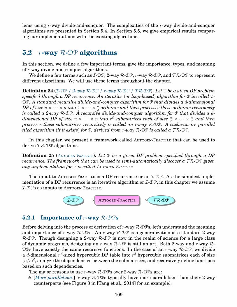
lems using r-way divide-and-conquer. The complexities of the r-way divide-and-conqueralgorithms are presented in Section 5.4. In Section 5.5, we give empirical results compar-ing our implementations with the existing algorithms.

5.2 r-way R-DP algorithmsIn this section, we define a few important terms, give the importance, types, and meaningof r-way divide-and-conquer algorithms.

We define a few terms such as I-DP, 2-wayR-DP, r-wayR-DP, and T R-DP to representdifferent algorithms. We will use these terms throughout the chapter.

Definition 24 (I-DP / 2-wayR-DP / r-wayR-DP / T R-DP). Let P be a given DP problemspecified through a DP recurrence. An iterative (or loop-based) algorithm for P is called I-DP. A standard recursive divide-and-conquer algorithm for P that divides a d-dimensionalDP of size n× · · · × n into n

2 × · · · ×n2 orthants and then processes these orthants recursively

is called a 2-way R-DP. A recursive divide-and-conquer algorithm for P that divides a d-dimensional DP of size n × · · · × n into rd submatrices each of size n

r× · · · × n

rand then

processes these submatrices recursively is called an r-way R-DP. A cache-aware paralleltiled algorithm (if it exists) for P, derived from r-way R-DP is called a T R-DP.

In this chapter, we present a framework called Autogen-Fractile that can be used toderive T R-DP algorithms.

Definition 25 (Autogen-Fractile). Let P be a given DP problem specified through a DPrecurrence. The framework that can be used to semi-automatically discover a T R-DP givenany implementation for P is called Autogen-Fractile.

The input to Autogen-Fractile is a DP recurrence or an I-DP. As the simplest imple-mentation of a DP recurrence is an iterative algorithm or I-DP, in this chapter we assumeI-DPs as inputs to Autogen-Fractile.

Autogen-FractileI-DP T R-DP

5.2.1 Importance of r-way R-DPsBefore delving into the process of derivation of r-way R-DPs, let’s understand the meaningand importance of r-way R-DPs. An r-way R-DP is a generalization of a standard 2-wayR-DP. Though designing a 2-way R-DP is now in the realm of science for a large classof dynamic programs, designing an r-way R-DP is still an art. Both 2-way and r-way R-DPs have exactly the same recursive functions. In the case of an r-way R-DP, we dividea d-dimensional nd-sized hypercubic DP table into rd hypercubic submatrices each of size(n/r)d, analyze the dependencies between the submatrices, and recursively define functionsbased on such dependencies.

The major reasons to use r-way R-DPs over 2-way R-DPs are:O [More parallelism.] r-way R-DPs typically have more parallelism than their 2-way

counterparts (see Figure 3 in [Tang et al., 2014] for an example).

109

O [Computer architectures that do not implement automatic page replacement or do notsupport recursion.] r-way R-DPs can be used to design highly efficient cache-awarealgorithms for computer architectures with deep memory hierarchy that do not im-plement automatic page replacement (e.g.: GPUs) or do not support recursion.

5.2.2 Types of r-way R-DPsIn the r-way R-DPs, the term r can be set to any of the three values as given below:

O r can be a constant.O r can be a function of n.O r can be the largest value tilesize[d] at every recursion level d based on a particular

cache or memory size such that the tile exactly fits in the memory.Typically, r is set to tilesize[d]. If there are h levels of memories or caches, then there

are h levels of recursion and hence there are h tile sizes tilesize[1 . . . h]. When a subproblemfits into a memory of the smallest size, we execute an iterative kernel.

If r is a constant or tilesize[d], then typically an r-way R-DP will have optimal serialI/O complexity (see Theorem 9). On the other hand, if r is a function of n and r is super-constant, then the r-way R-DP will have non-optimal serial I/O complexity. If r is a con-stant or a function of n, then the R-DP is cache-oblivious. If r is set to tilesize[d], thenthe R-DP is cache-aware. See Table 5.1 for a summary. In this paper, unless explicitlymentioned r-way R-DP means R-DP where r is set to tilesize[d].

Feature r = Θ (1) r = f(n) & r = ω (1) r = tilesize[d]Cache-obliviousness Yes Yes NoSerial I/O-optimality Yes (often) No Yes (often)

Table 5.1: Comparison of features of r-way R-DPs for different values of r.

5.2.3 GPU computing modelThe r-way R-DPs are ideally suited for computer architectures that do not implementautomatic page replacement schemes. The best example of such an architecture are theGPUs. Here, we give a brief overview of the GPU architecture, its programming model,and the challenges encountered when writing high-performing programs for the currentgeneration GPUs.

General purpose computing on GPUs. GPUs attached to CPU using PCI bus are usedas hardware accelerators. They have a many-core architecture having cores in the rangeof tens to hundreds. They are designed to have thousands of light-weight threads com-pared with those of the CPUs, are optimized for highly data-parallel and compute-intensivetasks, and are designed to maximize the throughput of the parallel programs. GPUs typ-ically have multiple types of parallelism: multithreading, single-instruction multiple-data(SIMD), and instruction-level parallelism. The GPU architecture is naturally suitable fordata-parallel scientific problems involving matrices of dimensions 1, 2, 3, or 4.

Figure 1 gives a simple representation of the memory hierarchy of the current genera-tion GPUs. The CPU is connected to a disk (or external-memory) of a very large size anda RAM (or internal-memory) of a decent size. The GPU consists of a global memory and

110

several shared memories. Each shared memory is connected to a constant number of coresthat have their own registers. A GPU is connected to the CPU through a PCI bus. MultipleGPUs can be connected to a single CPU.

Several application programming interfaces (APIs) have been developed so that pro-grammers can use GPUs for general purpose computing without being experts in com-puter graphics. The APIs are used to accelerate specific set of parallel computations onGPUs. Some of the most commonly used APIs are Open Computing Language (OpenCL),NVIDIA’s Compute Unified Device Architecture (CUDA), Microsoft’s DirectCompute, AMD’sAccelerated Parallel Processing (APP) SDK, and Open Accelerators (OpenACC). To exploitthe GPU architecture fully, the compute kernels must make use of the memory efficientlyand the organization of the threads must be good.

GPU programming challenges. Writing good GPU programs is hard. The difficulty inGPU programming is due to several factors.

O [Automatic page replacement is not implemented.] Automatic page replacement isnot implemented in GPUs. Recursive divide-and-conquer is a powerful tool to de-sign efficient (I/O-efficient, energy-efficient, and highly parallel), portable (cache- andprocessor-oblivious) and robust (cache- and processor-adaptive) algorithms. Howeverthese design techniques involve complicated control logic and hence they are eitherunsupported / unsuitable for GPUs, which forces programmers to search for otherapproaches.

O [GPU optimization is hard.] Optimization on GPUs is harder than that on CPUs.The key factors that have big influence on the performance on GPUs are: thread or-ganization (threads can be organized in blocks of different dimensions with differentdimension lengths), warp size (the granularity at which the streaming multiproces-sors can execute computations), memory coalescing (consecutive numbered threadsaccess consecutive memory locations), and streams and events (overlapping computekernel execution and data transfers). Depending on the mixture of optimizations usedthe performance can be drastically different.

5.3 The Autogen-Fractile frameworkIn this section, we present the Autogen-Fractile framework to design efficient tiled algo-rithms for a wide class of dynamic programs. From hereon, we call a recursive divide-and-conquer algorithm as an R-DP algorithm. The 2-way and r-way algorithms are called2-way and r-way R-DPs, respectively.

There are three major approaches in which the Autogen-Fractile framework could bedefined.

Example. For simplicity of exposition we explain the working of Autogen-Fractile bydesigning a T R-DP algorithm for Floyd-Warshall’s all-pairs shortest path (APSP) from itsrecurrence. The APSP is solved using the DP recurrence as described in Equation A.4 inAppendix A.3.

5.3.1 Approach 1: Generalization of 2-way R-DP

This is the first approach that uses the generalization of 2-way R-DPs to get r-way R-DPs.

111

The four main steps of Autogen-Fractile are:1. [2-way R-DP derivation.] A 2-way R-DP is constructed from a given I-DP.2. [3-way, 4-way, . . . R-DP derivation and visualizaton.] We derive r-way R-DP, where

r is a constant, and then visualize their working.3. [r-way R-DP derivation.] An r-way R-DP algorithm is derived with the aid of visual-

ization.4. [T R-DP derivation.] The T R-DP is derived for two consecutive memory levels from

the r-way R-DP by setting r based on the memory sizes.

2-way R-DP derivation

In this step, a 2-way R-DP algorithm is derived from a given I-DP. The major reason toderive 2-way R-DP is to identify the recursive functions that will be present in the 2-wayR-DP as the recursive functions in both 2-way and r-way R-DPs are exactly the same.

The structure and design of 2-wayR-DPs gives clues to the design of r-wayR-DPs. Thestandard 2-way R-DPs have been presented in [Chowdhury and Ramachandran, 2006,Chowdhury and Ramachandran, 2008, Chowdhury and Ramachandran, 2010] and otherwork. Such algorithms split a d-dimensional nd-sized hypercubic DP table into 2d hypercu-bic orthants each of size (n/2)d. They consist of a fixed number of distinct recursive func-tions and the functions are defined based on the dependencies between different orthants.Manually deriving 2-way R-DPs for several dynamic programs is difficult.

The Autogen [Chowdhury et al., 2016b] algorithm can be used to automatically discoverstandard 2-way (also r-way for small constant r) R-DPs for a wide class of dynamic pro-grams.2 By using Autogen, we can easily determine the number of recursive functions thatare present in the 2-way R-DP of a given dynamic program. Each recursive function isdifferent from each other in the order in which it writes and reads from submatrices of theinput DP table.

For example, we use Autogen to derive a 2-way R-DP for the Floyd-Warshall’s APSPproblem as described in Section 2.5.1. The 2-way R-DP is also described with diagramsin Section A.3. We see that there are four recursive functions A,B,C, and D. Each of therecursive functions take three parameters (X,U, V ). They three regions / submatrices arerelated to each other depending on which function calls them, as shown below.

O [Function A.] The relation is X = U and X = V .O [Function B.] The relation is X , U and X = V .O [Function C.] The relation is X = U and X , V .O [Function D.] The relation is X , U and X , V and U , V .

3-way, 4-way, . . . R-DP derivation and visualization

The Autogen algorithm can be used to automatically discover 3-way, 4-way, so on up tillany r-way R-DP, where r is a constant. The number of unique recursive functions in eachof the r-way R-DP will be the same. We use visualization to analyze the pattern behindhow the recursive functions updates different regions / submatrices of the DP table.

2Other types of cache-oblivious recursive algorithms [Frigo et al., 1999,Sibeyn, 2004,Cherng and Ladner,2005, D’Alberto and Nicolau, 2007] require problem-specific algorithm design logic and hence the approachmight not be generic enough to solve a large class of dynamic programs.

112

Consider Figure 5.2. It shows the order in which the A function of the r-way R-DP

for FW-APSP problem updates an n × n DP table for r = 2, 3, and 4. Similarly, we canwrite the updates of the B, C, and D functions. In the figure, the light pink, light red,light yellow, and light blue regions represent the submatrices updated by A, B, C, and D

functions, respectively. The numbers represent the relative order in which the functionswrite to regions. If two functions have the same numbers, it means they can write to theirrespective regions at the same time. If the time of one function is lesser than the another,then the former function must finish execution before the second function can start.

In the figure, when r = 2, then the ranges of k are[0, n2 − 1

], and

[n2 , n− 1

]. Similarly,

when r = 3, the ranges of k will be[0, n3 − 1

],[n3 ,

2n3 − 1

], and

[2n3 , n− 1

]. Similarly, k ranges

are defined for other values of r.The visualization of the function updates makes algorithm design easy. By analyzing

the regions (denoted by colors) written by different recursive functions and times at whichdifferent functions are invoked for different values of k and r, we can see the pattern.

𝐴0 𝐵1

𝐶1 𝐷2

𝐷5 𝐶4

𝐵4 𝐴3

𝑘 ∈ 0,𝑛

𝑟− 1

𝑟 = 2

𝐴0 𝐵1 𝐵1 𝐵1

𝐶1 𝐷2 𝐷2 𝐷2

𝐶1 𝐷2 𝐷2 𝐷2

𝐶1 𝐷2 𝐷2 𝐷2

𝐷5 𝐶4 𝐷5 𝐷5

𝐵4 𝐴3 𝐵4 𝐵4

𝐷5 𝐶4 𝐷5 𝐷5

𝐷5 𝐶4 𝐷5 𝐷5

𝐷8 𝐷8 𝐶7 𝐷8

𝐷8 𝐷8 𝐶7 𝐷8

𝐵7 𝐵7 𝐴6 𝐵7

𝐷8 𝐷8 𝐶7 𝐷8

𝐷11 𝐷11 𝐷11 𝐶10

𝐷11 𝐷11 𝐷11 𝐶10

𝐷11 𝐷11 𝐷11 𝐶10

𝐵10 𝐵10 𝐵10 𝐴9

𝐴0 𝐵1 𝐵1

𝐶1 𝐷2 𝐷2

𝐶1 𝐷2 𝐷2

𝐷5 𝐶4 𝐷5

𝐵4 𝐴3 𝐵4

𝐷5 𝐶4 𝐷5

𝐷8 𝐷8 𝐶7

𝐷8 𝐷8 𝐶7

𝐵7 𝐵7 𝐴6

𝑟 = 3 𝑟 = 4

𝑘 ∈𝑛

𝑟,2𝑛

𝑟− 1

𝑘 ∈2𝑛

𝑟,3𝑛

𝑟− 1

𝑘 ∈3𝑛

𝑟,4𝑛

𝑟− 1

Figure 5.2: The execution of the different functions invoked by the A function in r-wayR-DP of FW-APSP for r = 2, r = 3, and r = 4.

113

r-way R-DP derivation

Figure 5.2 gives a visualization of the updates of different functions invoked by the A

function of r-way R-DP in FW-APSP. We can derive an r-way R-DP from this visualizationby setting n = r and then analyzing. When we set r = 4, the updates of the four functionsare as shown in Figure 5.3.

In Figure 5.3, A,B,C, and D calls are shown in light pink, light red, light yellow, andlight blue. Consider the updates of the DP table by function A as shown in column 1 of theentire figure. When we look at all the pink cells, we see a pattern. The position of the pinkcells clearly depend on the value of k. To be exact, function A writes to cells at position(k, k). Immediately after A function call, functions B and C are invoked. Again, there is aclear-cut pattern. The B function calls are called on cells on the same row as that of A i.e.,(k, j), where j , k. Also, the C functions are called on cells on the same column as that of Ai.e., (i, k), where i , k. The function D is called on cells which have a different row and/orcolumn than k. That is the position of the D function calls are (i, j), where i , k and j , k.

𝐴0 𝐵1 𝐵1 𝐵1

𝐶1 𝐷2 𝐷2 𝐷2

𝐶1 𝐷2 𝐷2 𝐷2

𝐶1 𝐷2 𝐷2 𝐷2

𝐷5 𝐶4 𝐷5 𝐷5

𝐵4 𝐴3 𝐵4 𝐵4

𝐷5 𝐶4 𝐷5 𝐷5

𝐷5 𝐶4 𝐷5 𝐷5

𝐷8 𝐷8 𝐶7 𝐷8

𝐷8 𝐷8 𝐶7 𝐷8

𝐵7 𝐵7 𝐴6 𝐵7

𝐷8 𝐷8 𝐶7 𝐷8

𝐷11 𝐷11 𝐷11 𝐶10

𝐷11 𝐷11 𝐷11 𝐶10

𝐷11 𝐷11 𝐷11 𝐶10

𝐵10 𝐵10 𝐵10 𝐴9

𝐵1 𝐵1 𝐵1 𝐵1

𝐷2 𝐷2 𝐷2 𝐷2

𝐷2 𝐷2 𝐷2 𝐷2

𝐷2 𝐷2 𝐷2 𝐷2

𝐷5 𝐷5 𝐷5 𝐷5

𝐵4 𝐵4 𝐵4 𝐵4

𝐷5 𝐷5 𝐷5 𝐷5

𝐷5 𝐷5 𝐷5 𝐷5

𝐷8 𝐷8 𝐷8 𝐷8

𝐷8 𝐷8 𝐷8 𝐷8

𝐵7 𝐵7 𝐵7 𝐵7

𝐷8 𝐷8 𝐷8 𝐷8

𝐷11 𝐷11 𝐷11 𝐷11

𝐷11 𝐷11 𝐷11 𝐷11

𝐷11 𝐷11 𝐷11 𝐷11

𝐵10 𝐵10 𝐵10 𝐵10

𝐶1 𝐷2 𝐷2 𝐷2

𝐶1 𝐷2 𝐷2 𝐷2

𝐶1 𝐷2 𝐷2 𝐷2

𝐶1 𝐷2 𝐷2 𝐷2

𝐷5 𝐶4 𝐷5 𝐷5

𝐷5 𝐶4 𝐷5 𝐷5

𝐷5 𝐶4 𝐷5 𝐷5

𝐷5 𝐶4 𝐷5 𝐷5

𝐷8 𝐷8 𝐶7 𝐷8

𝐷8 𝐷8 𝐶7 𝐷8

𝐷8 𝐷8 𝐶7 𝐷8

𝐷8 𝐷8 𝐶7 𝐷8

𝐷11 𝐷11 𝐷11 𝐶10

𝐷11 𝐷11 𝐷11 𝐶10

𝐷11 𝐷11 𝐷11 𝐶10

𝐷11 𝐷11 𝐷11 𝐶10

𝐷2 𝐷2 𝐷2 𝐷2

𝐷2 𝐷2 𝐷2 𝐷2

𝐷2 𝐷2 𝐷2 𝐷2

𝐷2 𝐷2 𝐷2 𝐷2

𝐷5 𝐷5 𝐷5 𝐷5

𝐷5 𝐷5 𝐷5 𝐷5

𝐷5 𝐷5 𝐷5 𝐷5

𝐷5 𝐷5 𝐷5 𝐷5

𝐷8 𝐷8 𝐷8 𝐷8

𝐷8 𝐷8 𝐷8 𝐷8

𝐷8 𝐷8 𝐷8 𝐷8

𝐷8 𝐷8 𝐷8 𝐷8

𝐷11 𝐷11 𝐷11 𝐷11

𝐷11 𝐷11 𝐷11 𝐷11

𝐷11 𝐷11 𝐷11 𝐷11

𝐷11 𝐷11 𝐷11 𝐷11

𝑘 = 0

𝑘 = 1

𝑘 = 2

𝑘 = 3

Function 𝐴 Function 𝐵 Function 𝐶 Function 𝐷

Figure 5.3: The updates of the four functions in r-way R-DP of FW-APSP for n = r = 4.

We show in Figure A.7 an r-way R-DP for Floyd-Warshall’s APSP with 4 functions

114

A,B,C, and D. The initial invocation to the r-way R-DP is A(C,C,C, 1), where C is theDP table for the APSP problem. The term m in all the functions represents the dimensionlength at a particular recursion level. For function A, X = U = V . For function B, X , Uand X = V . Similarly, for function C, X = U and X , V . For function D, X , U , X , V ,and U , V . The keyword parallel means that the functions can be invoked in parallel. Inthis way, we design an r-way R-DP for Floyd-Warshall’s APSP.

T R-DP derivation

In this section, we explain how to port an r-way R-DP algorithm to a PMH model (seeSection 1.4.2) as shown in Figure 1.1. A similar kind of porting can be done for severaldynamic programs from the corresponding r-way R-DPs.

Let the r-way R-DP for a problem P consist of functions F1, . . . ,Fm such that any func-tion Fi, where i ∈ [1,m] calls other functions F|, where j ∈ [i,m].

Consider Figure 1.1 in Section 1.4.2. Let the input DP table be present in the memory atlevel h. This means that the data from the DP table has to pass through the memory levelsat h − 1, h − 2, . . . , 1 to reach the processors at level 0. We define the following functions:M[h]_F[1]_P, M[h-1]_F[1]_P, . . ., M[h-1]_F[m]_P, M[h-2]_F[1]_P, . . ., M[h-2]_F[m]_P, so ontill M[1]_F[1]_P, . . ., M[1]_F[m]_P. The brackets [ ] are simply used to demarcate numbersfrom alphabet and they are not considered as part of the function names. The terms F[1],. . ., F[m] correspond to the m recursive functions. The functions with keyword M[i], wherei ∈ [1, h] denotes that the input and the output matrices of the functions are present inmemory at level i.

Initially, the function M[h]_F[1]_P is invoked with the entire DP table as input. Thefunction splits the entire d-dimensional n × · · · × n DP table into rh × · · · × rh submatriceseach of size (n/rh) × · · · × (n/rh), assuming rh divides n for simplicity (and without loss ofgenerality). The term rh is chosen such that the input submatrices for the function exactlyfits a memory at level h− 1. The function copies the relevant submatrices to a (h− 1)-levelmemory and then invokes m other functions M[h-1]_F[1]_P, . . ., M[h-1]_F[m]_P as per ther-way R-DP algorithm and sends the desired submatrices as input parameters to thosechild functions. Note that we need not define functions M[h]_F[2]_P, . . ., M[h]_F[m]_P asthey will never be invoked.

The functions M[h-1]_F[1]_P, . . ., M[h-1]_F[m]_P split each of the (n/rh) × · · · × (n/rh)sized matrices present in level-(h − 1) memory into rh−1 × · · · × rh−1 submatrices eachof size (n/(rhrh−1)) × · · · × (n/(rhrh−1)), assuming rh−1 divides (n/rh) for simplicity. Thefunctions copy the relevant matrices to the (h − 2)-level memory and invoke the func-tions M[h-2]_F[1]_P, . . ., M[h-2]_F[m]_P. This process continues till we reach the functions:M[1]_F[1]_P, . . ., M[1]_F[m]_P. In these functions we run the iterative or looping kernelsand make use of threads to perform several computations. This is a high-level overviewof the division of work across recursive functions and memory levels. In this way, we candesign T R-DP algorithms from r-way R-DPs for a PMH model.

T R-DP for a GPU system. We explain how to port the r-way Floyd-Warshall’s APSPalgorithm given in Figure A.7 to a GPU system. For simplicity, we assume that the memoryhierarchy of our GPU system is as shown in Figure 5.1. It is easy to design algorithmsfor multiple levels, multiple GPUs, and multiple shared memories connected to a globalmemory.

115

Let the input DP table be present in the external memory. This means that the datafrom the DP table has to pass through three levels of memory: CPU RAM, GPU globalmemory, and GPU shared memory. We define the following functions: host_disk_A_FW,host_RAM_A_FW, . . ., host_RAM_D_FW, device_global_A_FW, . . ., device_global_D_FW, device_shared_A_FW,. . ., device_shared_D_FW. The terms A, B, C, and D correspond to the four recursive functions.The functions with keywords host and device represent that the code for such functionsrun on the CPU and GPU, respectively. The functions with keywords disk, RAM, global,and shared denote that the input and the output matrices of the functions are present inCPU disk, CPU RAM, GPU global memory, and GPU shared memory, respectively.

Initially, the function host_disk_A_FW is invoked with the entire DP table as input. Thefunction splits the entire n × n DP table into rd × rd submatrices each of size (n/rd) ×(n/rd), assuming rd divides n for simplicity (and without loss of generality). The termrd is chosen such that the input submatrices for the function exactly fits the RAM. Thefunction copies the relevant submatrices to RAM and then invokes four other functionshost_RAM_A_FW, . . ., host_RAM_D_FW as per the r-way R-DP algorithm and sends the desiredsubmatrices as input parameters to those child functions. Note that we need not definefunctions host_disk_B_FW, . . ., host_disk_D_FW as they will never be invoked.

The functions host_RAM_A_FW, . . ., host_RAM_D_FW split each of the (n/rd) × (n/rd) sizedmatrices present in RAM into rm × rm submatrices each of size (n/(rdrm)) × (n/(rdrm)),assuming rm divides (n/rd) for simplicity. The functions copy the relevant matrices to theGPU global memory and invoke the four functions device_global_A_FW, . . ., device_global_D_FW.This process continues till we reach the functions: device_shared_A_FW, . . ., device_shared_D_FW.In these functions we run the iterative or looping kernels and make use of threads to per-form several computations. This is a high-level overview of the division of work acrossrecursive functions and memory levels. In this way, we can design CPU-GPU algorithmsfrom r-way R-DPs.

Now let’s assume that we do not know the size of the CPU RAM, but it is maintained asfully associative memory with an automatic LRU page replacement policy. The input DPtable is stored in either the external memory or the RAM. Then instead of host_disk_A_FWand host_RAM_A_FW we will only have host_A_FW, and similarly host_B_FW, host_C_FW andhost_D_FW. Initially, the function host_A_FW is invoked with the entire DP table as input.The function splits the entire n× n DP table into 2× 2 subtables each of size (n/2)× (n/2),assuming n is divisible by 2 for simplicity. Now if a (n/2) × (n/2) subtable fits into theGPU global memory we invoke device_global_A_FW, . . ., device_global_D_FW, otherwisewe recursively invoke host_A_FW, . . ., host_D_FW.

5.3.2 Approach 2: Generalization of parallel iterative base cases

The five main steps of Autogen-Fractile are:1. [2-way R-DP derivation.] A 2-way R-DP is constructed from a given I-DP.2. [Serial iterative base cases construction.] Serial iterative base cases are constructed

for the recursive functions of the 2-way R-DP.3. [Parallel iterative base cases visualization.] Serial iterative base cases are constructed

for the recursive functions of the 2-way R-DP.4. [r-way R-DP derivation.] An r-way R-DP algorithm is derived with the aid of visual-

ization.

116

5. [T R-DP derivation.] The T R-DP is derived for two consecutive memory levels fromthe r-way R-DP by setting r based on the memory sizes.

2-way R-DP derivation

We derive a 2-way R-DP as explained in Section 5.3.1.

Serial iterative base cases construction

In this step, we construct the serial base cases for the recursive functions of the derived2-way R-DP. The serial base cases of both 2-way and r-way R-DPs are exactly the same.Also, the serial base cases give vital information regarding the recursive structure of ther-way R-DP.

For example, for the FW-APSP problem, the serial base cases of the four recursive func-tions A,B,C, and D of the 2-wayR-DP are shown in Figure 5.4. We assume that the initialdistance matrix consists of only non-negative values. It happened by luck that the serialbase cases for the four functions are the same. But, in general, the serial base cases of therecursive functions can be very different from each other.

The function Floop-FW takes several parameters. The parameters (xrow, xcol) are thestarting row and starting column of write region X. Similarly, (urow, ucol) and (vrow, vcol)are the starting rows and columns of read submatrices U and V , respectively. The value nis the dimension length of the submatrix X (or U or V ).

Floop-F W (xrow, xcol, urow, ucol, vrow, vcol, n)

1. for k ← 0 to n− 1 do2. for i← 0 to n− 1 do3. for j ← 0 to n− 1 do4. XI ← xrow + i;XJ ← xcol + j5. UI ← urow + i;V J ← vcol + j;K ← ucol + k6. D[XI,XJ ]← min D[XI,XJ ], D[UI,K] +D[K,V J ]

Figure 5.4: The serial base case of all recursive functions F ∈ A,B,C,D of 2-way R-DP

of FW-APSP assuming non-negative values for the initial distance matrix.

Constructing serial base cases for the recursive functions is majorly an art. By analyz-ing relationship between regions of a recursive function, we could attempt to come up withiterative kernels for updating the write regions from the read regions.

Parallel iterative base cases visualization

In this step, we visualize the execution of parallel iterative base cases of the recursivefunctions of the derived 2-way R-DP. Finding parallel iterative base cases is important aswe want to find parallel r-way R-DP.

We design parallel iterative base cases using the help of computers. Through goodvisualization we find the parallel versions of serial iterative base cases. Let every updateis of the form as given in Definition 4 in Section 2.2.1. Now, for each serial iterative basecase, for a specific value of n, we write the updates in the n×· · ·×n DP table using functionnames and time steps. If a cell x is written by reading u and v cells, then the write Ft at cellx, where F is the appropriate recursive function and t is the earliest time step at which F

117

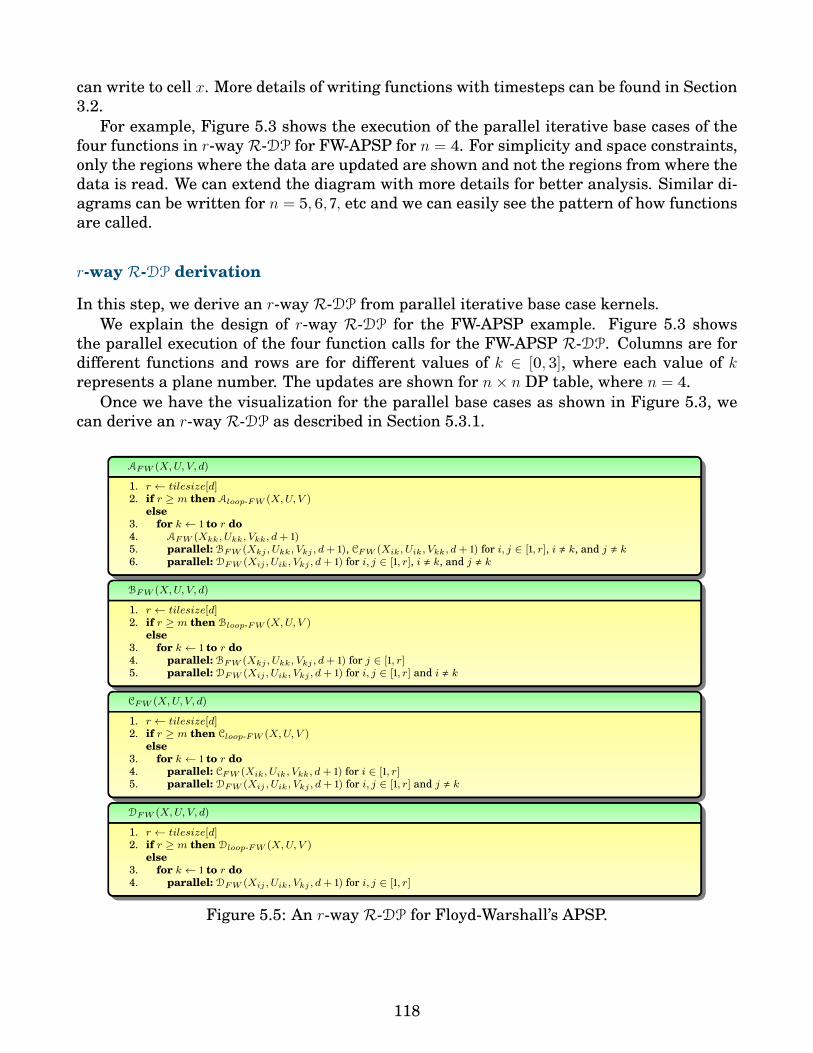
can write to cell x. More details of writing functions with timesteps can be found in Section3.2.

For example, Figure 5.3 shows the execution of the parallel iterative base cases of thefour functions in r-way R-DP for FW-APSP for n = 4. For simplicity and space constraints,only the regions where the data are updated are shown and not the regions from where thedata is read. We can extend the diagram with more details for better analysis. Similar di-agrams can be written for n = 5, 6, 7, etc and we can easily see the pattern of how functionsare called.

r-way R-DP derivation

In this step, we derive an r-way R-DP from parallel iterative base case kernels.We explain the design of r-way R-DP for the FW-APSP example. Figure 5.3 shows

the parallel execution of the four function calls for the FW-APSP R-DP. Columns are fordifferent functions and rows are for different values of k ∈ [0, 3], where each value of krepresents a plane number. The updates are shown for n× n DP table, where n = 4.

Once we have the visualization for the parallel base cases as shown in Figure 5.3, wecan derive an r-way R-DP as described in Section 5.3.1.

AF W (X,U, V, d)

1. r ← tilesize[d]2. if r ≥ m then Aloop-F W (X,U, V )

else3. for k ← 1 to r do4. AF W (Xkk, Ukk, Vkk, d+ 1)5. parallel: BF W (Xkj , Ukk, Vkj , d+ 1), CF W (Xik, Uik, Vkk, d+ 1) for i, j ∈ [1, r], i , k, and j , k6. parallel: DF W (Xij , Uik, Vkj , d+ 1) for i, j ∈ [1, r], i , k, and j , k

BF W (X,U, V, d)

1. r ← tilesize[d]2. if r ≥ m then Bloop-F W (X,U, V )

else3. for k ← 1 to r do4. parallel: BF W (Xkj , Ukk, Vkj , d+ 1) for j ∈ [1, r]5. parallel: DF W (Xij , Uik, Vkj , d+ 1) for i, j ∈ [1, r] and i , k

CF W (X,U, V, d)

1. r ← tilesize[d]2. if r ≥ m then Cloop-F W (X,U, V )

else3. for k ← 1 to r do4. parallel: CF W (Xik, Uik, Vkk, d+ 1) for i ∈ [1, r]5. parallel: DF W (Xij , Uik, Vkj , d+ 1) for i, j ∈ [1, r] and j , k

DF W (X,U, V, d)

1. r ← tilesize[d]2. if r ≥ m then Dloop-F W (X,U, V )

else3. for k ← 1 to r do4. parallel: DF W (Xij , Uik, Vkj , d+ 1) for i, j ∈ [1, r]

Figure 5.5: An r-way R-DP for Floyd-Warshall’s APSP.

118

T R-DP derivation

We derive the T R-DP from the R-DP as explained in Section 5.3.1.

5.4 Complexity analysisIn this section, we present the serial I/O complexity of r-way R-DPs on a parallel memoryhierarchy (PMH) model, I/O complexity of GPU algorithms on a typical GPU architecture,and the parallel running time of T R-DPs on the PMH model.

The parallel memory hierarchy (PMH) model was described in Section 1.4.2. Most ofour results are shown in the PMH model. The PMH model can be used in multi-cores ormany cores.

5.4.1 I/O complexityWe state the theorem for the I/O complexity of an r-way R-DP on a PMH model.

Theorem 9 (I/O complexity of r-way R-DPs on a PMH model). The serial I/Ocomplexity of an r-way R-DP on a PMH model for a d-dimensional hypercubic DPtable of size nd, where the parameter r is set to the best tile size at every recursionlevel, is

Q1(n) = O(

T1(n)BM (w/d)−1 + S(n)

B+ 1

)

where, T1(n) = total work = O (nw) , M = memory size, B = block size, M = Ω(Bd),

and S(n) = input DP table size = O(nd).

Proof. We prove the theorem in two stages:

(a) Q1(n) for r-way R-DP = Q1(n) for 2-way R-DP.The metric Q1(n) for an R-DP is computed as the product of number of subproblems thatexactly fits the cache of size M and the I/Os required to scan the input and output matricesfor a subproblem. Say r = 2k for some k ∈ N. Then, to compare the I/O complexities of thetwo algorithms, the r-way R-DP can be considered as simply the 2-way R-DP unrolled ktimes. The number of subproblems that exactly fit a memory of size M will be asymptoti-cally same for both 2-way and r-way R-DPs. Also, the I/Os required to scan the matricesthat exact fit the memory is asymptotically same for both 2-way and r-way R-DPs. Hence,the I/O complexity of 2-way and r-way R-DPs are the same.

Alternate argument. The claim can be proved in two steps. First, both 2-way and r-wayR-DPs exploit temporal locality from some constant factor of M . The reason for this isthat the r-way R-DP makes sure that every subproblem takes a constant fraction of thememory i.e., tile size is αM for some α ∈ (0, 1]. Similarly, the 2-way R-DP too exploitstemporal locality from constant fraction of the memory i.e., subproblem size is γM forsome γ ∈ (0, 1].

Second, both 2-way and r-way R-DPs are simply different scheduling of the same DPrecurrence and no DP cell update is applied more than once. Hence, the total work of the

119

2-way and r-wayR-DPs are the same. In both 2-way and r-wayR-DPs the amount of workdone for a subproblem when it fits into a memory of size M is asymptotically same due tothe previous arguments. Hence the proposition.

(b) Compute Q1(n) for 2-way R-DP.In a given r-way R-DP if we set r = 2 at every recursion level we get a 2-way R-DP. Oncewe have a 2-way R-DP we can simply use Theorem 2 from [Chowdhury et al., 2016b].

Theorem 2 from [Chowdhury et al., 2016b] is defined for the cache-oblivious model[Frigo et al., 1999]. The cache-oblivious model assumes automatic page replacement pol-icy. The theoretically optimal page replacement algorithm replaces the page (or data block)that will be used farthest in the future (which is difficult to predict). In practice, the leastrecently used (LRU) and first-in-first-out (FIFO) are the most commonly used page re-placement algorithms as they are within a factor of 2 of the optimal number of page re-placements. The current operating systems do not support automatic page replacementsbetween CPU RAM and GPU global memory or between two adjacent memory levels ofGPU. Still, it is possible to implement customized LRU or FIFO algorithms and simulatethe automatic page replacement policy. Hence, the serial I/O complexity bounds of ther-way R-DPs does not get affected without the automatic page replacement policies onCPU-GPUs.

Consider Floyd-Warshall’s APSP as an example. For f ∈ A,B,C,D, let Qf (n) denotethe serial I/O complexity of fFW of the 2-way R-DP on a matrix of size n × n. Also, γ bea constant such that γ ∈ (0, 1]. Then QA(n) = QB(n) = QC(n) = QD(n) = O (n2/B + n) ifn2 ≤ γM . On the other hand if n2 > γM , then

QA(n) = 2(QA

(n2

)+QB

(n2

)+QC

(n2

)+QD

(n2

))+ Θ (1)

QB(n) = 4(QB

(n2

)+QD

(n2

))+ Θ (1)

QC(n) = 4(QC

(n2

)+QD

(n2

))+ Θ (1)

QD(n) = 8QD

(n2

)+ Θ (1)

Applying Theorem 9, the serial I/O complexity of the r-wayR-DP of Floyd-Warshall’s APSPas shown in Figure A.7 is Q1(n) = O

(n3/

(B√M)

+ n2/B + 1).

We define a few terms before we present a theorem for the serial I/O complexity of GPUalgorithms. The theorem assumes that the core memory hierarchy of a GPU system is asshown in Figure 5.1, excluding intricate details. Let Mm, Mg, and Ms be the size of theCPU main memory, GPU global memory, and GPU shared memory, respectively. Let n,nm, ng, and ns be the subproblem parameter (i.e., tile dimension) when the subproblem ispresent in the disk, RAM, global, and shared memories, respectively. Then ndm = Θ (Mm),ndg = Θ (Mg) and nds = Θ (Ms). Let B, Bm, Bg, and Bs denote the block size between disk andRAM, RAM and global memory, global memory and shared memory, and shared memoryand processor, respectively. All M ’s, n’s, and B’s are natural numbers.

120

Theorem 10 (I/O complexity of GPU algorithms). The I/O complexity (numberof data blocks transferred) of an external-memory GPU algorithm when run on aGPU memory hierarchy as shown in Figure 5.1 between:

O disk & RAM is Θ(

nw

BMwd−1

m

+ nw

Mw+1

d−1

m

)

O RAM & global memory is Θ(

nw

BmMwd−1

g

+ nw

Mw+1

d−1

g

)

O global & shared memory is Θ(

nw

BgMwd−1

s

+ nw

Mw+1

d−1

s

)where, the total work of the GPU algorithm is Θ (nw).

Proof. First, we find the I/O complexity of the r-way R-DP between two adjacent levels ofmemories and then we directly use this result to prove the theorem.

Let the larger and smaller adjacent memories be of sizes ML and MS, respectively.Let the largest subproblem parameters that fit into ML and MS be integers nL and nS,respectively. Let BL denote the block size between larger and smaller memories. Thenumber of write and read submatrices for each recursive function of the R-DP is 1 + s,where s is a upper bounded by a constant. This is because there is only one regionto be written and there can be at most s distinct regions (not including the write re-gion) to be read from. Without loss of generality, we assume that an element takes 1byte. The space occupied by the (1 + s) read and write regions in the smaller memory is(1 + s)ndS ≤ MS, where nS ≤ (ML/(1 + s))1/d < nS + 1. Then the I/O complexity to fill thesmaller memory once is computed as O

(nd−1S (nS/BL + 1)

). The smaller memory will be

loaded Θ ((nL/nS)w) times. Hence, the I/O complexity between the larger and the smallermemories is O

((nL/nS)wnd−1S (nS/BL + 1)

).

We now apply the result above to prove the theorem. The I/O complexity between diskand RAM is O((n/nm)wnd−1m (nm/B + 1)). The I/O complexity between RAM and globalmemory to work on all data present in RAM is O((nm/ng)wnd−1g (ng/Bm + 1)). However, theRAM will be loaded Θ ((n/nm)w) times. Hence, the total I/O complexity between RAM andglobal is O((n/ng)wnd−1g (ng/Bm + 1)). We use a similar reasoning to compute the total I/Ocomplexity between global and shared memories. Substituting ndm = Θ (Mm), ndg = Θ (Mg)and nds = Θ (Ms) we obtain the claimed bounds.

5.4.2 Parallel running timeWe formalize a few ideas before we give a theorem on the parallel running time of the r-wayR-DPs on a parallel machine with deep memory hierarchy using space-bounded scheduler.

Let the recursive functions of an r-wayR-DP be F1, . . . ,Fm. Let us consider the recursivefunction calls any Fj makes when the data is in level i and is tiled for level i− 1 of the PMHhierarchy. Suppose Fj calls Fk a total of aij,k times from level i when pi = 1. If pi = ∞ thenFj will call as many recursive functions as possible in parallel, and let the number of suchparallel steps in which Fj makes at least one call to Fk is bij,k. Let A(i) and B(i) denote thelevel-i coefficient matrices (aij,k) and (bij,k), respectively. Let A and B be computed as:

A = A(h) ⊗A(h−1) ⊗ · · · ⊗A(1)

B = B(h) ⊗B(h−1) ⊗ · · · ⊗B(1)

121

where, ⊗ is a matrix multiplication operator.

Theorem 11 (Parallel running time of r-way R-DPs on a PMH model us-ing space bounded scheduler). Let the recursive functions of an r-way R-DP beF1, . . . ,Fm, and let A and B be as defined above. Then the parallel running time ofthe R-DP on a DP table of size nd under the PMH model with h+ 1 levels as definedabove will be:

T hPMH(n) = O(∑m

i=1 A[i, i]p

+m∑i=1

B[i, i])· Πh

i=1Bi

Proof. Suppose there are h levels of recursion. Let rh, . . . , r1 be the best tile sizes for recur-sion levels h to 1, respectively. This implies that n = rh × rh−1 × · · · × r1. The total spacecomplexity of the algorithm is assumed to be S(n) = Θ

(nd). Then,

ri =

Θ n

M1d

h−1

if i = h,

Θ((

Mi

Mi−1

) 1d

)if i ∈ [2, h− 1],

Θ(M

1d1

)if i = 1.

We assume for generality that it takes B time to write cells to a block of size B if thecells are computed from different processors.

An R-DP has only one recursive function. Let an r-way R-DP consist of only onefunction. Let the work and span of the function be defined by: T1(n) = aT1(n/r) + Θ (1)and T∞(n) = bT∞(n/r) + Θ (1) for a, b ≥ 1 and n ≥ r > 1. The work and span both areΘ (1) if n = 1. Let TPMH(n) be the parallel running time of the algorithm on a parallelmachine with the PMH memory model. We define T iPMH(n) to be the parallel running timeof the recursive function at level i. This implies TPMH(n) = T hPMH(n). Then, T iPMH(n) can becomputed recursively as:

T iPMH(n) =

O((

T1(r1)p1

+ T∞(r1))·B1

)if i = 1,

O((

T1(ri)pi

+ T∞(ri))·Bi

)· T i−1PMH( n

ri) if i ∈ [2, h].

Solving the recurrence, we get:

T hPMH(n) = Πhi=1O

((T1(ri)pi

+ T∞(ri))·Bi

)

An R-DP has multiple recursive functions. We extend the analysis above to multiplefunctions. Let the recursive functions of the r-way R-DP be F1, . . . ,Fm. Let the work andspan of an r-way recursive function Fj at level i be defined as: T i,Fj

1 (n) = ∑mk=1 a

ij,kT

i−1,Fk1 (n/ri)+

Θ (1) and Ti,Fj∞ (n) = ∑m

k=1 bij,kT

i−1,Fk∞ (n/ri) + Θ (1). As base cases, T 1,Fj

1 (r1) = ∑mk=1 a

1j,k and

T1,Fj∞ (r1) = ∑m

k=1 b1j,k. It is important to note that if the span of a function has maxx, y

term, then it is replaced with x+ y thereby this serves as an upper bound on span. Let the

122

parallel running time of the function Fj at level i be denoted by T i,Fj

PMH(n). Then we computeTi,Fj

PMH(n) recursively as:

Ti,Fj

PMH(n) =

O((

T1,Fj1 (r1)p1

+ T1,Fj∞ (r1)

)·B1

)if i = 1,

∑mk=1

(O((

aij,k

pi+ bij,k

)·Bi

)· T i−1,Fk

PMH ( nri

))

if i ∈ [2, h].

Let A(i) and B(i) denote the level-i coefficient matrices (aij,k) and (bij,k), respectively. LetA and B be computed as:

A = A(h) ⊗A(h−1) ⊗ · · · ⊗A(1)

B = B(h) ⊗B(h−1) ⊗ · · · ⊗B(1)

where, ⊗ is a matrix multiplication operator. Solving the parallel running time recurrence,we get:

T hPMH(n) = O(∑m

i=1 A[i, i]p

+m∑i=1

B[i, i])· Πh

i=1Bi

5.5 Experimental resultsIn this section, we present empirical results showing the performance benefits of our GPUalgorithms that are based on r-way R-DP. The internal-memory GPU algorithms areimplemented by Stephen Tschudi and the external-memory GPU algorithms are imple-mented by Rathish Das.

5.5.1 Experimental setupAll our experiments were performed on a heterogeneous node of Stampede supercomputer.The multicore machine had a dual-socket 8-core 2.7 GHz Intel Sandy Bridge processors(2× 8 = 16 cores in total) and 32 GB RAM. Each core was connected to a 32 KB private L1cache and a 256 KB private L2 cache. All cores in a processor shared a 20 MB L3 cache.For GPGPU processing the Stampede compute nodes were attached with a single NVIDIAK20 GPU on each node. Each GPU had an on-board GDDR5 memory of 5GB. The GPUmachine had 2496 CUDA cores for parallel processing.

All our algorithms were implemented in C++. We used Intel Cilk Plus extension toparallelize and Intelő C++ Compiler v13.0 to compile the CPU implementations with opti-mzation parameters -O3 -ipo -parallel -AVX -xhost. We used NVIDIA’s CUDA platformto write our GPU programs. The programs were compiled with nvcc compiler with param-eters -O3 -gencode arch=compute_35,code=sm_35.

5.5.2 Internal-memory GPU implementationsWe focus on four DP problems: Floyd-Warshall’s APSP, Gaussian elimination without piv-oting, parenthesis problem, and the gap problem. The programs with cpu and gpu keywords

123

are run on CPU and GPU machines, respectively. The different types of programs we com-pare are:

(i) cpu-idp: iterative serial program,(ii) cpu-rdp: standard 2-way parallel R-DP,

(iii) gpu-rdp: r-way parallel R-DP.For the FW problem, we also have

(iv) gpu-tidp-harish: Harish and Narayanan’s [Harish and Narayanan, 2007] tiled-iterativeprogram,

(v) gpu-tidp-lund: Lund and Smith’s [Lund and Smith, 2010] tiled-iterative program,(vi) gpu-tidp-katz: Katz and Kider’s [Katz and Kider Jr, 2008] tiled-iterative program,

(vii) gpu-rec-buluc: Buluc et al.’s implementation of the 2-way R-Kleene algorithm withVolkov and Demmel’s optimization [Volkov and Demmel, 2008] for the MM kernel,

(viii) gpu-rdp-opt: r-way R-DP replaced with Buluc et al.’s MM-like3 kernel for the MM-like functions of the R-DP.

Optimizations. The common optimizations used for the programs, except cpu-idp, are asfollows.

(i) We use shared memory of the GPUs by setting BLOCK_SIZE = 32 so that 1024 threadscould work on square matrices of size 32 × 32 simultaneously. Also, two blocks with1024 threads were run in parallel.

(ii) If a function kernel reads from submatrices it is not writing to (MM-like), then we donot use synchronization inside the kernel.

(iii) Row-major order was used for all submatrices instead of column-major order. Flip-ping a submatrix to column-major degrades performance. We used row-major or-der for the grid and also inside each block inside a grid. Using row-major acrossBLOCK_SIZE × BLOCK_SIZE worsens the performance.

(iv) Allocating memory using gpuMalloc() on GPU global memory is slow. Instead ofinvoking this function multiple times we simply malloc once and then copy the sub-matrices to the respective regions.

(v) We allocate directly in host’s pinned memory using cudaMallocHost(). This reducesthe block transfers between pageable host memory and pinned memory.

The cpu-idp was not optimized. The optimizations used for cpu-rdp include:(i) #pragmas such as #pragma parallel, #pragma ivdep, and min loop count(B),

(ii) using 64 byte-aligned matrices,(iii) write optimizations,(iv) using pointer arithmetic,(v) Z-morton layout (only for the gap problem).

The optimizations used for the gpu-rdp programs are: (i) block-row-major order (similaras in the case of tiling) to reduce data transfers, (ii) GRID_SIZE was set to min n, 16384,where 16384 was the maximum size such that our subproblems can exactly fit into the5GB of global memory, (iii) The data copy from RAM to global memory and vice versawas synchronized. Using asynchronous copy (overlapping computations and data copy) isextremely complicated.

There are a few important points related to the programs of the FW problem. The threetiled-iterative implementations were blocked for 32 × 32 instead of 16 × 16 as set in the

3MM = Matrix Multiplication

124

original versions. The A,B, and C functions in the tiled implementations were optimizedas much as possible, whereas the D function was already optimized.

Results. Figure 5.6 shows the speedup of various programs w.r.t. cpu-idp for four DPproblems. For each program, the DP table dimension n is varied from 210 to 215. Whenn = 215, a subproblem fits in RAM, and in all other cases the subproblems fit in GPUglobal memory. For FW-APSP, gpu-rdp-opt was the second fastest running program with aspeedup of 219×, whereas gpu-rec-buluc had a speedup of 330× for n = 215. This is becauseunlike gpu-rec-buluc, all the kernels of gpu-rdp-opt were not MM-like and hence it ranslower than Buluc et al.’s implementation.

For the Gaussian elimination, parenthesis and gap problems for n = 215, the speedupof our gpu-rdp programs were 216×, 1762×, and 523×, respectively, way higher than theircpu-rdp counterparts which were 169×, 162×, and 188×, respectively. The speedup of theGPU algorithms for the parenthesis and gap problems is more than that for FW-APSP /Gaussian elimination because of two reasons:

(i) cpu-idp for the former two problems do not have spatial locality whereas the lattertwo have spatial locality,

(ii) gpu-rdp for the former two problems have higher parallelism than the latter two.

5.5.3 External-memory GPU implementationsIt is easy to extend our algorithms to work for external-memory (or disks). We could useeither 2-way or r-way R-DPs for external-memory until a subproblem fits in GPU globalmemory, after which we use r-way R-DPs. To make our algorithms RAM-oblivious, we use2-way R-DPs in the external-memory until a subproblem fits in GPU global memory. Wehave implemented algorithms for all four problems: Floyd-Warshall’s APSP, parenthesis,gap, and Gaussian elimination. We use Standard Template Library for Extra Large DataSets (STXXL) [STX, ] 1.4.1 to implement our algorithms for external-memory. STXXL isa C++ library for implementing containers and algorithms that can process vast amountsof data that reside in disks. In STXXL, we set the external block size as 4MB, #pages as1024, and #blocks per page as 1. This gives the RAM size as 4GB.

For each of the four DP problems we compare three programs:(a) cpu-rdp-1: 2-way serial R-DP running on CPU,(b) cpu-rdp-128: 2-way parallel R-DP running on CPU with 128 cores (the details of

which is explained shortly),(c) gpu-rdp: r-way parallel R-DP running on the GPU machine.

The input DP table is stored in Z-morton-row-major layout in the external-memory suchthat when a submatrix reaches a size that fits in the GPU global memory it is stored in row-major order. Note that the input problem consists of a single matrix in external-memory.On the other hand, a subproblem can consist of multiple submatrices (e.g. up to 3 matricesfor the R-DP of FW-APSP) of the input DP table and they all have to fit into the GPUglobal memory and this is taken care by the recursive functions of the r-way R-DPs. Oncewe compute a DP table submatrix, we write the output to the same location in the DPtable in the external-memory. For the CPU programs, the base case dimension length forthe algorithms was set to 256 and we run iterative kernels inside each base case.

The running time of cpu-rdp-1 and cpu-rdp-128 are approximated as follows. The DPtable is stored as a grid of blocks, each block is of size 16K×16K and it is stored in Z-morton

125

order. We use r-way R-DP4 in external-memory and whenever a subproblem is brought toRAM, we use 2-way R-DP to execute it on CPU.

Let nbase, n128base, nchunk, tbase, tchunk represent the number of invocations to base case ker-

nels, number of parallel steps of execution of the base case kernels when we assume 128cores, number of times RAM (of size 16K × 16K) is loaded and unloaded, minimum timetaken (among several runs) to execute a base case kernel, and time taken to copy databetween external-memory and RAM as given in STXXL I/O statistics, respectively. Then,running time of cpu-rdp-1 is (nbase · tbase + nchunk · tchunk). The running time of cpu-rdp-128is (n128

base · tbase + nchunk · tchunk).

Results. Figure 5.7 shows the speedup of various programs w.r.t. cpu-rdp-1 for four DPproblems. For each program, the DP table dimension n is varied from 215 to 217. In all cases,the input matrices are stored in the external-memory. For FW-APSP, Gaussian elimina-tion, parenthesis and gap problems for n = 217, the speedup of our gpu-rdp programs were3072×, 1096×, 3376×, and 1122×, respectively, way higher than their cpu-rdp-128 counter-parts which were 126×, 126×, 112×, and 122×, respectively.

1248

163264

128256512

1024 2048 4096 8192 16384 32768

Spe

edu

p

n

FW-APSP - Speedup

cpu-rdp gpu-rec-buluc gpu-rdp gpu-rdp-opt

gpu-tidp-harish gpu-tidp-lund gpu-tidp-katz

2

4

8

16

32

64

128

256

1024 2048 4096 8192 16384 32768

Spee

du

p

n

Gaussian elimination - Speedup

cpu-rdp gpu-rdp

2

8

32

128

512

2048

1024 2048 4096 8192 16384 32768

Spe

edu

p

n

Parenthesis - Speedup

cpu-rdp gpu-rdp

1

4

16

64

256

1024

1024 2048 4096 8192 16384 32768

Spe

edu

p

n

Gap problem - Speedup

cpu-rdp gpu-rdp

Figure 5.6: Speedup of cpu-rdp and gpu-rdp programs over cpu-idp for various dynamicprograms. For FW-APSP, the speedup of gpu-buluc-rec and gpu-rdp-opt are also shown.

5.6 Conclusion and open problemsWe presented a framework called Autogen-Fractile to semi-automatically discover recur-sively tiled algorithms based on r-way recursive divide-and-conquer that are efficient in

4We did not make the program RAM-oblivious to make the benchmark program run fastest.

126

64

128

256

512

1024

2048

4096

8192

32768 65536 131072

Spe

edu

p

n

FW-APSP - Speedup

cpu-rdp-128 gpu-rdp cpu-max-speedup

64

128

256

512

1024

2048

32768 65536 131072

Spe

edu

p

n

Gaussian elimination - Speedup


32

64

128

256

512

1024

2048

4096

32768 65536 131072

Spe

edu

p

n

Parenthesis - Speedup


64

128

256

512

1024

2048

4096

32768 65536 131072Sp

eed

up

n

Gap problem - Speedup


Figure 5.7: Speedup of cpu-rdp-128 and gpu-rdp programs w.r.t. cpu-rdp-1 for variousdynamic programs in external-memory.

computer architectures that do not support recursion. We develop several efficient algo-rithms for GPUs using our framework and achieve high performance and beat almost allthe existing implementations.

A few open problems are:O [Automation of Autogen-Fractile framework.] Completely automate the derivation of

formulas and looping constraints for designing the r-way R-DPs.

127

Chapter 6

Semi-Automatic Discovery ofDivide-&-Conquer DP Algorithms withSpace-Parallelism Tradeoff

In chapter 2, we presented the Autogen algorithm to automatically discover divide-and-conquer DP algorithms. In chapter 3, we presented the Autogen-Wave framework to im-prove the parallelism of these auto-discovered algorithms to near-optimal. In this chapter,we will see a framework called Autogen-Tradeoff that can be used to improve the paral-lelism of certain class of the Autogen-discovered algorithms by increasing the space usage.

The standard in-place divide-and-conquer parallel matrix multiplication algorithm usesΘ (p log n) extra space (in the worst case) including stack space (where p = #threads) andhas Θ (n2) parallelism. On the other hand, the not-in-place divide-and-conquer parallelmatrix multiplication algorithm uses Θ

(p1/3n2

)extra space, but achieves high parallelism

of Θ(n3/ log2 n

). The more space we use, the more parallelism we can exploit. So, there

exists a tradeoff between total space and parallelism.We present the Autogen-Tradeoff framework that can be used to improve the paral-

lelism of a class of divide-and-conquer cache-oblivious matrix algorithms by increasing thespace. As an application of the framework, we present a hybrid matrix multiplication al-gorithm, which is a careful mix of the two algorithms above, to achieve parallelism ω (n2)using total space of Θ (n2+ε) for some ε ∈ (0, 1). Similarly, we give hybrid algorithms toasymptotically increase the parallelism for other algorithms such as multi-instance Viterbialgorithm, Floyd-Warshall’s all-pairs shortest path, and protein folding problems.

Our experiments show that when we have enough space and thousands of processors,these hybrid algorithms will be able to harness more parallelism to achieve good perfor-mance.

6.1 IntroductionMulticore machines often have a tree-like cache hierarchy consisting of different-sizedcaches having various access times. The access times of caches farther from the proces-sors are an order of magnitude times that of caches near to the processors. Reducing thenumber of data movements for an algorithm across different levels of the cache hierarchy

128

invariably reduces the running time of the algorithm. To achieve this, when programsbring data to cache, they must do as much work as possible before evicting the data out ofcache. Hence, achieving good cache locality improves the overall performance of an algo-rithm.

Present-day multicore machines have more than one processing element (ranging from2 to 80) to execute a program in parallel decreasing its overall running time. More thenumber of processors, the faster the algorithm runs. To exploit parallelism, it is not justenough to have more processing elements but the algorithm must have asymptoticallymore parallelism as well. Good cache locality and good parallelism are the two key factorsto increase the performance of a parallel algorithm. Also, if a parallel algorithm has to beportable i.e., be able to run on machines from smart phones to compute nodes of supercom-puters without modification then the algorithm has to be resource-oblivious (e.g.: cache-and processor-oblivious).

The cache-oblivious recursive divide-and-conquer parallel algorithms highly parallel,and exploit several optimization opportunities. By this virtue, if properly implemented,they can be both high-performing and portable at the same time. But, one importantquestion remains. Can we increase the parallelism of these algorithms?

Space-parallelism tradeoff. We build on top of a simple space-parallelism tradeoff ideato show that with extra space we can increase the parallelism of the cache-oblivious divide-and-conquer parallel algorithms asymptotically. This idea works for several problemssuch as matrix multiplication, multi-instance Viterbi algorithm, Floyd-Warshall’s all-pairsshortest path, and protein accordion folding.

Consider an example. Given an array of n numbers, its sum can be found in a couple ofdifferent ways without altering the input array (see Table 6.1):

1. [Sequential sum.] The sum is found by simply adding all the numbers using Θ (1)extra space and it has a span of Θ (n) (or a parallelism of Θ (1)) as the algorithm isinherently sequential.

2. [Parallel reduction.] The sum is found using parallel reduction using Θ (n) extra spaceand it has a span of Θ (log n) (or a parallelism of Θ (n/ log n)). See Figure 6.1.

Work Span Parallelism ExtraAlgorithm (T1) (T∞) (T1/T∞) space (S∞)Sequential sum (in-place) Θ (n) Θ (n) Θ (1) Θ (1)Parallel reduction (not-in-place) Θ (n) Θ (log n) Θ (n/ log n) Θ (n)Hybrid algorithm 1 (not-in-place) Θ (n) Θ ((n/r) log r) Θ (r/ log r) Θ (r)Hybrid algorithm 2 (not-in-place) Θ (n) Θ ((n/r) + log r) Θ (nr/(n+ r log r)) Θ (r)

Table 6.1: Space-parallelism tradeoff for sum of an array. For the hybrid algorithm, r ∈[2, n].

It is straightforward to see that we can have a space-parallelism tradeoff for the algo-rithm above. When we increase the extra space from Θ (1) to Θ (n), the span decreases fromΘ (n) to Θ (log n) or the parallelism increases from Θ (1) to Θ (n/ log n).

We can construct two types of hybrid algorithms using the basic algorithms. We assumethat we are allowed Θ (r) extra space, where r ∈ [2, n]. The two hybrid algorithms usingthe allowed extra space are:

129

Figure 6.1: Computing sum of an array using parallel reduction.

1. [Hybrid algorithm 1: Serial on parallel.] We divide the array of size n into Θ (n/r)chunks. For each of the Θ (n/r) chunks we apply the parallel reduction method. Thesum of numbers in each chunk is computed in parallel. However, the chunks are pro-cessed in a serial fashion. The span for computing sum in each chunk is Θ (log r).There are Θ (n/r) chunks. Hence, the total span is Θ ((n/r) log r). Parallelism isΘ (r/ log r).

2. [Hybrid algorithm 2: Parallel on serial.] We divide the array of size n into Θ (r)chunks. For each of the Θ (r) chunks we apply the serial sum method. The sum ofnumbers in each chunk is computed serially. However, the chunks are processed ina parallel fashion using parallel reduction method. The span for computing sum ineach chunk is Θ (n/r). There are Θ (r) chunks. Using a parallel reduction method, thetotal span will be Θ ((n/r) + log r). Parallelism is Θ (nr/(n+ r log r)).

Figure 6.2: Pictorial representation of the two hybrid algorithms to compute the sum ofelements of an array. Left: Hybrid algorithm 1: Serial on parallel. Right: Hybrid algorithm2: Parallel on serial.

We extend this idea further to matrix multiplication. There are two major ways tomultiply matrices using divide-and-conquer (see Figure 6.3):

1. In-place algorithm denoted by AMM

2. Not-in-place algorithm denoted by AMM -N

The AMM algorithm has optimal Q1(n) = Θ(n3/(B

√M)

), has decent span of T∞(n) =

Θ (n), and uses extra space of Θ (p log n) including stack space. On the other hand, the

130

AMM -N algorithm has optimal Q1(n) = Θ(n3/(B

√M)

)but, has a small span of T∞(n) =

Θ(log2 n

), and uses extra space of O

(p1/3n2

). Using the space-parallelism tradeoff idea, we

can get hybrid algorithms for matrix multiplication and other problems.We develop a hybrid algorithm AMM -H following a careful combination of AMM and

AMM -N . We execute AMM -N for a few levels in the recursion tree (say, k levels) until theproblem size reduces to a threshold at which we switch and execute AMM . When we haveenough processors and space, the hybrid algorithm AMM -H is better than both AMM andAMM -N in parallelism by guaranteeing a complexity of T∞(n) = O

(k(2 log n− k) + n/2k

),

Sp(n) = O(minp1/3, 2kn2

), where Sp(n) denotes the total space when there are p pro-

cessors. This tradeoff can be applied to other problems such as multi-instance Viterbialgorithm, Floyd-Warshall’s all-pairs shortest path, and protein accordion folding. Thecomplexities of all algorithms are summarized in Table 6.2.

In further sections, we present a framework called Autogen-Tradeoff that can be usedto derive hybrid algorithms that have asymptotically higher parallelism than that for stan-dard divide-and-conquer matrix algorithms.

Algorithm Work Span Space(T1) (T∞) (Sp)

MM in-place Θ (n3) Θ (n) O (n2)MM not-in-place Θ (n3) Θ

(log2 n

)O(p1/3n2

)MM hybrid Θ (n3) Θ

(k(2 log n− k) + n

2k

)O(minp1/3, 2kn2

)VA in-place Θ (n3t) Θ (tn) O (n2)VA not-in-place Θ (n3t) Θ

(t log2 n

)O(p1/3n2

)VA hybrid Θ (n3t) Θ

(t(k(2 log n− k) + n

2k

))O(minp1/3, 2kn2

)Table 6.2: Work (T1), serial cache complexity (Q1), and span (T∞) of in-place, not-in-place, andhybrid algorithms for matrix problems. and parallelism (T1/T∞) of I-DP and R-DP algorithms forseveral DP problems. Here, n = problem size, t = #timesteps, and p = #cores. We assume that theDP table is too large to fit into the cache. On p cores, the running time is Tp = O (T1/p + T∞) withhigh probability when run under the randomized work-stealing scheduler.

Our contributions. The major contributions of this chapter are:1. [Algorithmic.] We present a generic framework called Autogen-Tradeoff to develop

recursive divide-and-conquer matrix algorithms that often have a tradeoff betweenspace and parallelism. We derive these hybrid algorithms from standard cache-oblivious divide-and-conquer DP algorithms. We present four hybrid algorithms forfour problems: matrix multiplication, Floyd-Warshall’s all-pairs shortest path, andprotein accordion folding that exploit the tradeoff. See Table 6.2.

2. [Experimental.] We present empirical results to show that the hybrid algorithmsindeed increase parallelism with very small degradation in cache performance.

Organization of the chapter. Section 6.2 presents the space-parallelism tradeoff frame-work Autogen-Tradeoff. The empirical evaluations for the algorithms are presented inSection 6.3.

131

6.2 The Autogen-Tradeoff frameworkIn this section, we describe the tradeoff between space and parallelism for cache-obliviousrecursive parallel algorithms considering matrix multiplication as an example. A similartechnique can be applied to other problems to asymptotically increase parallelism usingasymptotically more space.

Example. Consider matrix multiplication (MM). MM is one of the most fundamental andwell-studied problems in mathematics and computer science. Due to its extensive usein scientific computing, several algorithms have been proposed to solve the problem inparallel and distributed systems. In this paper, we focus on the square MM problem withcubic computations.

The classic square MM problem is defined as follows. Given two n × n matrices Aand B containing real numbers and stored in row- and column-major orders, respectively,the matrix product of A and B, denoted by C, is computed through C[i, j] = ∑n

1 A[i, k] ×B[k, j]. The naive cache-inefficient iterative algorithm is in-place has a span of Θ (n) or aparallelism of Θ (n2). The tiled cache-efficient cache-aware algorithm with tile size

√M

has Θ (n) span or Θ (n2) parallelism.

Assumptions. We make the following assumptions:O The cache is tall i.e., M = Ω (B2).O Data layout is row-major order.O Task scheduler is randomized work stealing.

Parallel cache complexity. If we use a randomized work stealing scheduler, the par-allel cache complexity of a recursive divide-and-conquer algorithm on a p-processor ma-chine can be found using the formula Qp(n) = O (Q1(n) + p(M/B)T∞(n)) w.h.p. in theproblem parameter. The maximum realistic value p can take is same as the parallelismi.e., T1(n) ÷ Tp(n). When we substitute the maximum value of p in Qp equation, we getQ∞(n) = O (Q1(n) + (T1(n)/T∞(n))(M/B)T∞(n)) = O (Q1(n) + T1(n)M/B) = O (T1(n)M/B) >Q1(n). Hence, Q∞(n) will always be greater than Q1(n) and is bounded by O (T1(n)M/B).

Framework. The four main steps of Autogen-Tradeoff are:1. [In-place algorithm construction.] An in-place divide-and-conquer algorithm is gener-

ated using Autogen for a given problem. See Section 6.2.1.2. [Span analysis.] If the span recurrence of the in-place algorithm satisfies a particular

property then a hybrid algorthm can be found. See Section 6.2.2.3. [Not-in-place algorithm construction.] A not-in-place algorithm is derived from the

in-place algorithm using extra space. See Section 6.2.3.4. [Hybrid algorithm construction.] A hybrid algorithm with asymptotic increase in

parallelism is constructed with space usage somewhere between in-place and not-in-place algorithms. See Section 6.2.4.

6.2.1 In-place algorithm constructionIn this step, we construct an in-place divide-and-conquer algorithm to a given matrix prob-lem.

We can generate in-place 2-way recursive divide-and-conquer algorithms to a wide class

132

of dynamic programs and matrix problems, including matrix multiplication, using Auto-gen. Please refer to Chapter 2 for more details.

Consider the matrix multiplication problem. The in-place cache-efficient cache-obliviousrecursive parallel algorithm for square matrices was developed in [Blumofe et al., 1996a]and then extended to rectangular matrices in [Prokop, 1999]. From hereon, we consideronly square matrices unless explicitly mentioned. The in-place algorithm is shown in Fig-ure 6.3, function AMM . The term ` in AMM represents the plane number. This means thatthe algorithm updates the `th plane through the base case looping kernels (Aloop−MM). Thevalue of ` can be set to 0 when we are using the in-place algorithm independently. Theusage of term ` becomes clear when we analyze the hybrid algorithm. Lemma 2 gives thecomplexity analysis of the in-place MM algorithm.

Lemma 2 (In-place MM). The in-place MM algorithm AMM , assuming a tall cache,has a complexity of T1(n) = Θ (n3), Q1(n) = Θ

(n3/(B

√M) + n2/B + n

), T∞(n) =

Θ (n), S∞(n) = Θ (n2), and Ep(n) = Θ (p log n).

Proof. The recurrences for the complexities are as follows:

T1(n) =

Θ (1) if n = 1,8T1(n2 ) + Θ (1) if n > 1. Q1(n) =

Θ(n2

B+ n

)if n2 ≤ αM,

8Q1(n2 ) + Θ (1) if n2 > αM.

T∞(n) =

Θ (1) if n = 1,2T∞(n2 ) + Θ (1) if n > 1.

S∞(n) =

O (1) if n = 1,4S∞(n2 ) + Θ (1) if n > 1.

Also, for p processors, there can be at most p tasks running in parallel. When the tasksreach the basecase, they execute Aloop-MM . As each executing task is a leaf node in therecursion tree, we might require a total extra space all along the path from the root to thep executing leaves of the recursion tree. Hence, Ep(n) = Θ (p log n). Solving the recurrencesand from Ep(n) argument, we have the lemma.

6.2.2 Span analysisIn this section, we give a theorem that relates to the span of the in-place algorithm. If thein-place algorithm satisfies a particular property as given in the span theorem (Theorem12), then a hybrid algorithm can be designed to asymptotically increase the parallelism.

Theorem 12 (Span analysis). Let F1,F2, . . . ,Fm be the m functions of the autogen-erated in-place R-DP. Let the span of the functions be computed as follows:

TFi(n) =

1 if n = 1,∑mj=i aijTFj

(n/2) + Θ (1) otherwise;(6.1)

where, TFi(n) is the span of Fi(n) and aij is the number of parallel steps in which

the function Fi(n) calls Fj(n). Suppose the function Fm be like matrix-multiplicationreading from submatrices it does not write to and also that Fm is dominating (seeDefinition 16). Also, let maximum = maxa11, a22, . . . , amm.

If maximum = 2, then there exist not-in-place and hybrid algorithms to asymp-totically increase parallelism.

133

Proof. Let P = Fr1 ,Fr2 , . . . ,F|P | be a path in the recursion tree of the root (= Fr1 = F1) toa node corresponding to Fm(= F|P |). Let q out of these |P | functions call themselves in(maximum = 2) parallel steps and q is maximized over all possible paths in the recursiontree. Then the span of the in-place algorithm is

TF1(n) = Θ(n logq−1 n

)(in-place algorithm) (6.2)

which is found by recursively applying the master theorem from the leaf of the recursiontree to the root.

We know that Fm is matrix multiplication algorithm (or any matrix-multiplication-likekernel) and there is a not-in-place algorithm for it whose span recurrence is

TFm(n) = TFm

(n

2

)+ Θ (1) if n > 1. (6.3)

It is important to note that replacing the in-place MM-like algorithm Fm with a not-in-place algorithm, the value of q will be decremented by 1. This gives rise to the not-in-placealgorithm with span

TF1(n) =

Θ (log n) if q = 1,Θ(n logq−1 n

)if q > 1.

(6.4)

This implies that there is a not-in-place algorithm with asymptotic decrease in span (orasymptotic increase in parallelism). Hence, there is a hybrid algorithm with asymptoticincrease in parallelism.

Consider the MM example. We see that the in-place MM has only one function and itcalls itself in two parallel steps as shown in the proof of Lemma 2. It satisfies Theorem 1and hence a not-in-place and a hybrid algorithm exist for MM.

6.2.3 Not-in-place algorithm constructionIn this step, we show how to construct a not-in-place algorithm via the MM example.

For DP or DP-like divide-and-conquer algorithms, we can easily construct the not-in-place algorithms by simply replacing the in-place MM-like functions with the not-in-placeversions of them.

Consider Figure 6.3. The AMM -N algorithm is the not-in-place algorithm. Instead ofcomputing the 8 matrix products in 2 parallel steps, we compute the 8 matrix products in1 parallel step. This requires us to compute the products in a different matrix and oncewe have the 8 matrix products in 2 different tables, we combine them to form the originalsolution. This requires extra space that can be either dynamically allocated during exe-cution or statically allocated at before the initial call to the algorithms. Dynamic memoryallocation inside the MM function calls is not recommended because of memory contention.Lemma 3 gives the complexity analysis for the not-in-place MM.

Lemma 3 (Not-in-place MM). The not-in-place MM algorithm AMM -N , assuminga tall cache, has a complexity of T1(n) = Θ (n3), Q1(n) = Θ

(n3/(B

√M) + n2/B + n

),

T∞(n) = Θ(log2 n

), Sp(n) = Θ

(n2p1/3

).

134

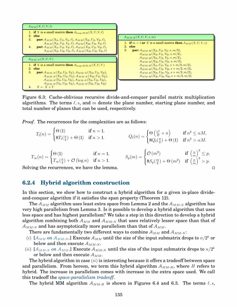
AMM (X,U, V, `)

1. if X is a small matrix then Aloop-MM (X,U, V, `)2. else3. par: AMM (X11, U11, V11, `), AMM (X12, U11, V12, `),

AMM (X21, U21, V11, `), AMM (X22, U21, V12, `)4. par: AMM (X11, U12, V21, `), AMM (X12, U12, V22, `),

AMM (X21, U22, V21, `), AMM (X22, U22, V22, `)

AMM -N (X,U, V )

1. if X is a small matrix then Aloop-MM -N (X,U, V )2. else3. par: AMM -N (X11, U11, V11), AMM -N (X12, U11, V12),

AMM -N (X21, U21, V11), AMM -N (X22, U21, V12),AMM -N (Y11, U12, V21), AMM -N (Y12, U12, V22),AMM -N (Y21, U22, V21), AMM -N (Y22, U22, V22)

4. X ← X + Y

AMM -H(X,U, V, s,m)

1. if m = 1 or X is a small matrix then AMM (X,U, V, s)2. else3. par: AMM -H(X11, U11, V11, s,m/2),

AMM -H(X12, U11, V12, s,m/2),AMM -H(X21, U21, V11, s,m/2),AMM -H(X22, U21, V12, s,m/2),AMM -H(X11, U12, V21, s+m/2,m/2),AMM -H(X12, U12, V22, s+m/2,m/2),AMM -H(X21, U22, V21, s+m/2,m/2),AMM -H(X22, U22, V22, s+m/2,m/2)

Figure 6.3: Cache-oblivious recursive divide-and-conquer parallel matrix multiplicationalgorithms. The terms `, s, and m denote the plane number, starting plane number, andtotal number of planes that can be used, respectively.

Proof. The recurrences for the complexities are as follows:

T1(n) =

Θ (1) if n = 1,8T1(n2 ) + Θ (1) if n > 1. Q1(n) =

Θ(n2

B+ n

)if n2 ≤ αM,

8Q1(n2 ) + Θ (1) if n2 > αM.

T∞(n) =

Θ (1) if n = 1,T∞(n2 ) +O (log n) if n > 1.

Sp(m) =

O (m2) if(nm

)3≤ p,

8Sp(m2 ) + Θ (m2) if(nm

)3> p.

Solving the recurrences, we have the lemma.

6.2.4 Hybrid algorithm constructionIn this section, we show how to construct a hybrid algorithm for a given in-place divide-and-conquer algorithm if it satisfies the span property (Theorem 12).

The AMM algorithm uses least extra space from Lemma 2 and the AMM -N algorithm hasvery high parallelism from Lemma 3. Is it possible to develop a hybrid algorithm that usesless space and has highest parallelism? We take a step in this direction to develop a hybridalgorithm combining both AMM and AMM -N that uses relatively lesser space than that ofAMM -N and has asymptotically more parallelism than that of AMM .

There are fundamentally two different ways to combine AMM and AMM -N :(i) [AMM on AMM -N .] Execute AMM until the size of the input submatrix drops to n/2k or

below and then execute AMM -N .(ii) [AMM -N on AMM .] Execute AMM -N until the size of the input submatrix drops to n/2k

or below and then execute AMM .The hybrid algorithm in case (ii) is interesting because it offers a tradeoff between space

and parallelism. From hereon, we term this hybrid algorithm AMM -H , where H refers tohybrid. The increase in parallelism comes with increase in the extra space used. We callthis tradeoff the space-parallelism tradeoff.

The hybrid MM algorithm AMM -H is shown in Figures 6.4 and 6.3. The terms `, s,

135

level = 0

level = k

level = log n

Execute

AMM

Execute

AMM-N

Figure 6.4: Hybrid matrix multiplication algorithm.

and m in AMM -H denote the starting plane number and total number of planes that canbe used, respectively. The way the algorithm works is that we execute the not-in-placealgorithm (i.e., AMM -N ) until the problem size or the task size reduces to a threshold value,say (n/2k)× (n/2k) for some k, and then we execute the in-place algorithm (i.e., AMM ).

In AMM -H , the more number of levels we execute AMM -N initially, the more space weconsume, the more parallelism we have. Therefore, we need to carefully choose the levelk in which we need to shift from one algorithm to another. The complexity of the AMM -Halgorithm is given in Theorem 13.

Theorem 13 (Hybrid MM). The hybrid MM algorithm AMM -H , assuming a tallcache, has a complexity of T1(n) = Θ (n3), Q1(n) = O

(n3/(B

√M) + n2/B + n

),

T∞(n) = O(k(2 log n− k) + n/2k

), and Sp(n) = O

(minp1/3, 2kn2

).

Proof. In the hybrid MM algorithm AMM -H , when the size of each input matrix drops ton/2k or below then we execute AMM . Hence, in the following recurrences, when the prob-lem size reaches the base case (i.e., when m = n/2k), the complexities are same as thecomplexities from Lemma 2 but n is replaced by n/2k. Also, the recursion cases are fromLemma 3. Thus, we have:

T1(m) =

Θ((

n2k

)3)if m = n

2k ,

8T1(m2 ) + Θ (1) if m > n2k .

Q1(m) =

Θ(

n3

8kB√M

+ n2

4kB+ n

2k

)if m = n

2k ,

8Q1(m2 ) + Θ (1) if m > n2k .

T∞(m) =

Θ(n2k

)if m = n

2k ,

T∞(m2 ) +O (logm) if m > n2k .

Sp(m) =

O (m2) if m = n2k or

(nm

)3≤ p,

8S(m2 ) + Θ (m2) if m > n2k and

(nm

)3> p.

Solving the recurrences and from Sp(n) argument, we have the theorem.

Theorem 13 may or may not be cache-efficient depending on the value of k.

136

6.3 Experimental resultsIn this section, we present empirical results1 showing the increased parallelism of ourhybrid algorithms.

Experimental setup. All our experiments were performed on a multicore machine withdual-socket 8-core 2.7 GHz Intel Sandy Bridge processors (2 × 8 = 16 cores in total) and32 GB RAM. Each core was connected to a 32 KB private L1 cache and a 256 KB privateL2 cache. All cores in a processor shared a 20 MB L3 cache. All algorithms were imple-mented in C++. We used Intel Cilk Plus extension to parallelize and Intelő C++ Compilerv13.0 to compile all implementations with optimzation parameters -O3 -ipo -parallel

-AVX -xhost. PAPI 5.3 [PAP, ] was used to count cache misses.

Implementations. We implement algorithms for the matrix multiplication (MM) prob-lem. For all programs, the base case size B was set to 32. For MM, the DP table dimensionn varied from 26 = 64 to 212 = 2048.

For each problem, we compared five algorithms: in-place algorithm I, not-in-place algo-rithm N, and three hybrid algorithms H(2), H(4), H(8). The hybrid algorithm H(m) meansthat the algorithm uses a total of m planes each of size n × n. In other words, m − 1 extraplanes were used along with the input DP table. We can think of the in-place algorithm asH(1) and not-in-place algorithm as H(n).

Matrix multiplication. The plots of MM are shown in Figure 6.5. The parallelism of I isΘ (n2) and that of N is Θ

(n3/ log2 n

). Hence, the difference between the values of I and N

increases significantly when n increases. The more number of planes we use in the hybridalgorithm, the more parallelism we can exploit. The cache misses incurred by a hybridalgorithm is almost the same as that of the in-place algorithm.

6.4 Conclusion and open problemsWe presented a framework called Autogen-Tradeoff to semi-automatically design recur-sive divide-and-conquer algorithms with very high parallelism using extra space. Theframework can be useful when we have enough number of processors and enough space.

A few open problems are:O [Improve span analysis.] Improve the framework such that given a DP recurrence,

find whether the problem can have an algorithm with parallelism better than that ofthe standard 2-way R-DP or not. If we can indeed get better parallelism, derive thefaster algorithm.

O [Tight lower bounds for optimal parallelism.] The optimal parallelism of an algo-rithm can be different depending on the constraints. Identify different constraints foran algorithm (e.g.: with and without using exra space), and prove lower bounds foroptimal parallelism.

O [Compute optimal parallelism.] For any given DP recurrence, compute the optimalparallelism achievable by an algorithm (irrespective of all constraints) that can beused to solve a DP recurrence.

1The matrix multiplication algorithm was implemented by Mohammad Mahdi Javanmard.

137

2

16

128

1024

8192

65536

524288

6 4 1 2 8 2 5 6 5 1 2 1 0 2 4 2 0 4 8

PA

RA

LLEL

ISM

DP TABLE DIMENSION N (B = 32)

MM - PARALLELISM

I N H(2) H(4) H(8)

2

8

32

128

512

2048

8192

32768

6 4 1 2 8 2 5 6 5 1 2 1 0 2 4 2 0 4 8

BU

RD

ENED

PA

RA

LLEL

ISM

DP TABLE DIMENSION N (B = 32)

MM - BURDENED PARALLELISM

I N H(2) H(4) H(8)

256

1024

4096

16384

65536

262144

1048576

6 4 1 2 8 2 5 6 5 1 2 1 0 2 4 2 0 4 8

L3 C

AC

HE

MIS

SES

DP TABLE DIMENSION N (B = 32, P = 16)

MM - L3 CACHE MISSES

I N H(2) H(4) H(8)

Figure 6.5: Performance comparison of in-place algorithm - I, not-in-place algorithm - N,hybrid algorithms with k planes H(k) where k = 2, 4, 8: (a) parallelism, (b) burdened paral-lelism, and (c) L3 cache misses; when DP table dimension increases and base case size Bis 32.

138

Appendix A

Efficient Divide-&-Conquer DPAlgorithms

In this section, we present several divide-and-conquer DP algorithms. By the virtue ofdivide-and-conquer (see Section 1.7), these algorithms are cache-efficient, cache-oblivious,processor-oblivious, and parallel. Standard 2-way divide-and-conquer algorithms for longestcommon subsequence, parenthesis problem, sequence alignment with gap penalty (oftencalled the gap problem), and Floyd Warshall’s all-pairs shortest path already exist and weinclude them here for completeness and we analyze them in more depth. The rest of thealgorithms are new.

We also discuss the divide-and-conquer variants of elementary sorting algorithms. Thoughsuch algorithms are not DP algorithms, the core approach of designing those algorithmscomes from Autogen.

A.1 Longest common subsequence & edit distanceA sequence Z = 〈z1, z2, . . . zk〉 is called a subsequence of another sequence X = 〈x1, x2, . . . xm〉if there exists a strictly increasing function f : [1, 2, . . . , k] → [1, 2, . . . ,m] such that for alli ∈ [1, k], zi = xf(i). A sequence Z is a common subsequence of sequences X and Y if Zis a subsequence of both X and Y . In the longest common subsequence (LCS) problem,we are given two sequences X and Y , and we need to find a maximum-length commonsubsequence of X and Y . The LCS problem arises in a wide variety of applications, and itis especially important in computational biology in sequence alignment.

Given two sequences X = 〈x1, x2, . . . xm〉 and Y = 〈y1, y2, . . . yn〉, we define C[i, j] (0 ≤ i ≤m, 0 ≤ j ≤ n) to be the length of an LCS of 〈x1, x2, . . . xi〉 and 〈y1, y2, . . . yj〉. Then C[m,n]is the length of an LCS of X and Y , and can be computed using the following recurrencerelation (see, e.g., [Cormen et al., 2009]):

C[i, j] =

0 if i = 0 or j = 0,C[i− 1, j − 1] + 1 if i, j > 0 and xi = yj,max C[i, j − 1], C[i− 1, j] if i, j > 0 and xi , yj.

(A.1)

The classic dynamic programming solution to the LCS problem is based on this recur-rence relation, and computes the entries of C[0 . . .m, 0 . . . n] in row-major order in Θ (mn)time and space.

139

LOOP-LCS(C)

1. for i← 0 to n do C[i, 0]← 0; C[0, i]← 02. for i← 1 to n do3. for j ← 1 to n do4. if xi = yj then C[i, j]← C[i− 1, j − 1] + 15. else C[i, j]← max (C[i, j − 1], C[i− 1, j])

PAR-LOOP-LCS(C)

1. C[0, 0]← 02. parallel for i← 1 to n do C[i, 0]← 0; C[0, i]← 03. for t← 1 to n do4. parallel for j ← 1 to t do5. i← t− j − 16. if xi = yj then C[i, j]← C[i− 1, j − 1] + 17. else C[i, j]← max (C[i, j − 1], C[i− 1, j])8. for t← n+ 1 to 2n− 1 do9. parallel for j ← t− n+ 1 to n do

10. i← t− j + 111. if xi = yj then C[i, j]← C[i− 1, j − 1] + 112. else C[i, j]← max (C[i, j − 1], C[i− 1, j])

ALCS(X)

1. if X is a small matrix then Aloop-LCS(X)2. else3. ALCS(X11)4. parallel: ALCS(X12), ALCS(X21)5. ALCS(X22)

Figure A.1: The dependency graph, serial iterative algorithm, parallel iterative algorithm,and the divide-and-conquer algorithm for the LCS problem. Initial call to the algorithm isALCS(C), where C is the full DP table.

Please refer Figure A.1. It shows the dependency graph for the problem. A cell atposition (i, j) depends on three light green cells as per the recurrence. The figure containsseveral algorithms for computing the LCS lengths. A simple iterative algorithm is givenas LOOP-LCS. A highly parallel iterative algorithm is given as PAR-LOOP-LCS.

The divide-and-conquer algorithm ALCS was presented in [Chowdhury and Ramachan-dran, 2006, Chowdhury and Ramachandran, 2008]. A picture representation of algorithmis shown in the right of Figure A.1. The algorithm splits the entire DP X table into fourquadrants: X11 (top-left), X12 (top-right), X21 (bottom-left), and X22 (bottom-right). Comput-ing the LCS lengths in each of these quadrants are the independent subproblems of ouroriginal problem (computing the entire DP table). Hence, we solve them recursively. First,we fill X11. Then we fill quadrants X12 and X21 in parallel. Finally, we fill X22. Note thatthe quadrants are filled recursively. More details on the algorithm can be found in thecorresponding paper(s).

The problem of converting one string to another string using three operations: inserts,

140

deletes, and substitutions, and minimizing the overall cost is called the edit distance prob-lem [Leiserson, 2010]. The applications of the edit distance problem include automaticspelling correction and the longest common subsequence. The LCS problem is in fact aspecial case of the edit distance problem. A quadratic-time algorithm to find the edit dis-tance between two strings is given in [Wagner and Fischer, 1974]. A sub-quadratic timealgorithm for the problem was first presented in [Masek and Paterson, 1980]. The divide-and-conquer algorithm presented for the LCS problem also works and retains its optimalserial cache complexity for the edit distance problem provided cost for inserts, deletes,and substitutions are fixed constants. If the costs for the three operations are extremelygeneric, then no cache-efficient divide-and-conquer algorithm exists for the problem.

Linear space. Note that if we use Θ (n2) space for the DP table, as the total work (to-tal number of computations) is also Θ (n2), we cannot get temporal locality and the serialcache complexity will be Θ (n2/B). To exploit temporal locality, the total work complexitymust be asymptotically greater than the total space complexity. We can exploit temporallocality if we asymptotically reduce the space. As described in the papers [Chowdhuryand Ramachandran, 2006,Chowdhury and Ramachandran, 2008], we store only the inputboundaries for different parallel tasks (or quadrants of the DP table) that are to be exe-cuted. With this idea, the space can be reduced to Θ (n log n). To reduce the space further tolinear space i.e., Θ (n) space, we must reuse the input / output boundaries of the quadrantsacross different levels of the recursion tree.

Complexity analysis for the PAR-LOOP-LCS algorithmThe parallel iterative algorithm makes use of a 2-D matrix C for simplicity. The algorithmcan be modified easily to make use of a 1-D array of size Θ (n).

For f ∈ PAR-LOOP-LCS, let Wf (n), Qf (n), Tf (n), and Sf (n) denote the total work,serial cache complexity, span, and parallel space consumption of fLCS for the parametern. Then Wf (n) = Θ (n2). Qf (n) is same as scanning n anti-diagonals n times i.e., Qf (n) =Θ(n(nB

+ 1))

= Θ(n2

B+ n

). Each parallel for loop takes Θ (log n) time to divide the loop to

processors and there are Θ (n) such parallel for loops. Hence, Tf (n) = Θ (n log n). SpaceSf (n) is simply Θ (n).

For the edit distance and LCS problems, the PAR-LOOP-LCS algorithm achievesT1(n) = Θ (n2), Q1(n) = Θ

(n2

B+ n

), T∞(n) = Θ (n log n), parallelism = Θ

(n

logn

), and

S∞(n) = Θ (n).

Complexity analysis for the 2-way ALCS algorithmFor f ∈ A, let Wf (n), Qf (n), Tf (n), and Sf (n) denote the total work, serial cache complex-ity, span, and parallel space consumption of fLCS for the parameter n. Then

WA(n) =O (1) if n = 1,4WA

(n2

)+ Θ (1) otherwise; QA(n) =

O(nB

+ 1)

if n ≤ γAM ,4QA

(n2

)+ Θ (1) otherwise;

TA(n) = Θ (1) if n = 1,

3TA(n2

)+ Θ (1) otherwise; SA(n) =

O (n) if n ≤ γAM ,2SA

(n2

)+ Θ (n) otherwise;

141

where, γA is a suitable constant. Solving, WA(n) = Θ (n2), QA(n) = Θ(n2

BM+ n2

M2 + nB

+ 1),

TA(n) = Θ(nlog 3

), and SA(n) = Θ (n log n).

The space complexity is Θ (n log n) because there are Θ (log n) levels in the recursion treeand at every level the input boundaries take Θ (n) space. In fact, we can reduce the spaceto Θ (n) if at every level we reuse the input boundaries of the parent function call.

For the edit distance and LCS problems, the 2-way divide-and-conquer algorithmachieves T1(n) = Θ (n2), Q1(n) = Θ

(n2

BM+ n2

M2 + nB

+ 1), T∞(n) = Θ

(nlog 3

), parallelism

= Θ(n2−log 3

), and S∞(n) = Θ (n).

Complexity analysis for the r-way ALCS algorithmIn an r-way divide-and-conquer algorithm, we divide the entire n × n matrix into r × rsubmatrices each of size (n/r)×(n/r) and solve them recursively. In Figure A.1, for an r-waydivide-and-conquer we will have r2 function calls inside the ALCS function. For simplicityof exposition we assume that n is a power of r. When r increases, the number of cache missesincreases, the span decreases, and it gets more difficult to implement the program.

For f ∈ A, let Wf (n), Qf (n), Tf (n), and Sf (n) denote the total work, serial cache com-plexity, span, and parallel space consumption of r-way fLCS for the parameter n. Then

WA(n) =O (1) if n = 1,r2WA

(nr

)+ Θ (1) otherwise; QA(n) =

O(nB

+ 1)

if n ≤ γAM ,r2QA

(nr

)+ Θ (1) otherwise;

TA(n) = Θ (1) if n = 1,

(2r − 1)TA(nr

)+ Θ (1) otherwise; SA(n) =

O (n) if n ≤ γAM ,rSA

(nr

)+ Θ (n) otherwise;

where, γA is a suitable constant. Solving,WA(n) = Θ (n2),QA(n) = O(

n2

BdM/re + n2

dM/re2 + nB

+ 1)

,

TA(n) = O(nlogr(2r−1)

), and SA(n) = Θ (n logr n).

The serial cache complexity is found as below

QA(n) ≤ r2QA

(n

r

)+ c = r2

(r2QA

(n

r2

)+ c

)+ c = (r2)2QA

(n

r2

)+ cr2 + c

= (r2)kQA

(n

rk

)+ c(r2)k−1 + · · ·+ c

(say

n

rk≤ γAM

)= c(r2)k

(n

rkB+ 1

)+ c

((r2)k−1 + · · ·+ 1

)= crk

n

B+ c

((r2)k + · · ·+ 1

)= crk

n

B+ c

((r2)k+1 − 1r2 − 1

)≤ crk

n

B+ c′r2k (for some constant c′)

We would like to find the upper bound for QA(n). As(n/rk

)≤ γAM , we have

(n/rk−1

)>

γAM , or rk−1 < (n/(γAM)). Substituting for the upper bound of rk−1 in the inequality above

142

we get

QA(n) ≤ cn

B· rk−1 · r + c′

(rk−1

)2· r2 ≤ c

n

B· n

γAM· r + c′

(n

γAM

)2

· r2

= O(n2r

BM+ n2r2

M 2

)= O

n2

B⌈Mr

⌉ + n2⌈Mr

⌉2

When r increases, the temporal cache locality decreases, and hence the number of cachemisses increases. The amount of memory from which we can exploit temporal locality isbM/rc for the r-way divide-and-conquer LCS algorithm. Hence, the serial cache complexityis a function of n, B, and bM/rc.

The span can be computed easily

TA(n) ≤ (2r − 1)TA(n

r

)+ c = (2r − 1)

((2r − 1)TA

(n

r

)+ c

)+ c

= (2r − 1)2TA(n

r2

)+ c ((2r − 1) + 1)

= (2r − 1)kTA(n

rk

)+ c

((2r − 1)k−1 + · · ·+ 1

) (say

n

rk= 1

)= (2r − 1)kc+ c′(2r − 1)k−1 = c′(2r − 1)k = c′(2r − 1)logr n = O

(nlogr(2r−1)

)The space complexity is Θ (n logr n) because there are Θ (logr n) levels in the recursion

tree and at every level the input boundaries take Θ (n) space. Again, we can reduce thespace to Θ (n) if at every level we reuse the input boundaries of the parent function call.

For the edit distance and LCS problems, the r-way divide-and-conquer algorithmachieves T1(n) = Θ (n2), QA(n) = O

(n2

BdM/re + n2

dM/re2 + nB

+ 1)

, TA(n) = O(nlogr(2r−1)

),

parallelism = Θ(n2−logr(2r−1)

), and S∞(n) = Θ (n).

A.2 Parenthesis problemThe parenthesis problem [Galil and Park, 1994] is defined by the following recurrencerelation:

C[i, j] =xj if 0 ≤ i = j − 1 < n,mini<k<j (C[i, k] + C[k, j]) + w(i, j, k) if 0 ≤ i < j − 1 < n; (A.2)

where xj ’s are assumed to be given for j ∈ [1, n]. We also assume that w(·, ·, ·) is a functionthat can be computed in-core without additional memory accesses.

The class of problems defined by the recurrence relation above includes optimal chainmatrix multiplication, RNA secondary structure prediction, optimal binary search trees,optimal polygon triangulation, string parsing for context-free grammar (CYK algorithm),optimal natural join of database tables (Selinger algorithm), maximum perimeter inscribed

143

polygon, and offline job scheduling minimizing flow time of jobs. A variant of this recur-rence which does not include the w(i, k, j) term and is defined as the simple dynamic pro-gram, was considered in [Cherng and Ladner, 2005].

As in [Cherng and Ladner, 2005], instead of recurrence A.2 we will use the followingslightly augmented version of A.2 which will considerably simplify the recursive subdivi-sion process in our divide-and-conquer algorithm.

C[i, j] =

∞ if 0 ≤ i = j ≤ n,xj if 0 ≤ i = j − 1 < n,mini<k≤j (C[i, k] + C[k, j]) + w(i, j, k) if 0 ≤ i < j − 1 < n;

(A.3)

where w(i, j, k) is defined to be ∞ when k = i or k = j. It is straightforward to see thatrecurrences A.2 and A.3 are equivalent, i.e., they compute the same values for any givenC[i, j], 0 ≤ i < j − 1 < n. In the rest of this section we will assume for simplicity thatn = 2` − 1 for some integer ` ≥ 0.

Please refer Figure A.2. It gives the dependency graph for the parenthesis problem. Acell (i, j) depends on the light green cells. Cell numbered k on the horizontal light green lineis paired with cell numbered k on the vertical light green line during the update of cell (i, j).A serial iterative algorithm LOOP-PARENTHESIS and a parallel iterative algorithm PAR-LOOP-PARENTHESIS are also given in the figure. PAR-LOOP-PARENTHESIS completelyupdates the cells of the diagonals (with slope -1) in the DP table from left to right.

A divide-and-conquer algorithm [Chowdhury and Ramachandran, 2008] (both pseu-docode and pictorial representation) are shown in Figure A.2. The algorithm consists ofthree recursive divide-and-conquer functions named Apar, Bpar and Cpar. The three func-tions differ from each other in their functionalities. Function Apar(X) completely updatesa right-triangular region X by reading from itself; Bpar(X,U, V ) updates a square regionX by reading from itself and two other right-triangular regions U and V ; and finally thefunction Cpar(X,U, V ) updates a square region X by reading from two other square regionsU and V .

The work done by each of the base case kernels: Aloop−par,Bloop−par, and Cloop−par is cubicw.r.t. their input parameter. The number of function calls to Aloop−par,Bloop−par, and Cloop−parare Θ (n) ,Θ (n2), and Θ (n3), respectively. This means that if we optimize only the base caseCloop−par then we can get large performance gains. Another important point to note is thatthe kernel Bloop−par is more flexible than Aloop−par. Similarly, kernel Cloop−par is more flexiblethan Bloop−par.

Complexity analysis for the PAR-LOOP-PARENTHESIS algorithmFor f ∈ PAR-LOOP-PARENTHESIS, let Wf (n), Qf (n), Tf (n), and Sf (n) denote the work,serial cache complexity, span, and space consumption of fpar on a matrix of size n × n.The total work remains same compared to the serial algorithm Wf (n) = Θ (n3). Qf (n)can be computed for the three loops as Qf (n) = Θ (n · n · (n)) = Θ (n3). The third loopi.e., k-loop accesses data from both horizontal or vertical lines. Therefore, irrespectiveof whether we use row-major order or column-major order, we cannot get spatial localityfor the innermost loop. The span is computed as Tf (n) = Θ (n · (log n+ n · (1))) = Θ (n2).Finally, Sf (n) = Θ (n2).

144


1. for i← n− 1 to 0 do2. for j ← i+ 2 to n do3. for k ← i+ 1 to j do4. C[i, j]← min

(C[i, k] + C[k, j]

+w(i, j, k), C[i, j]

)PAR-LOOP-PARENTHESIS(C, n)

1. for t← 2 to n− 1 do2. parallel for i← 1 to n− t do3. j ← t+ i4. for k ← i+ 1 to j do5. C[i, j]← min

(C[i, k] + C[k, j]

+w(i, j, k), C[i, j]

)Apar(X)

1. if X is a small matrix then Aloop-par(X)2. else3. parallel: Apar(X11), Apar(X22)4. Bpar(X12, X11, X22)

Cpar(X,U, V )

1. if X is a small matrix then Cloop-par(X,U, V )2. else3. parallel: Cpar(X11, U11, V11), Cpar(X12, U11, V12),

Cpar(X21, U21, V11), Cpar(X22, U21, V12)4. parallel: Cpar(X11, U12, V21), Cpar(X12, U12, V22),

Cpar(X21, U22, V21), Cpar(X22, U22, V22)

Bpar(X,U, V )

1. if X is a small matrix then Bloop-par(X,U, V )2. else3. Bpar(X21, U22, V11)4. parallel: Cpar(X11, U12, X21), Cpar(X22, X21, V12)5. parallel: Bpar(X11, U11, V11), Bpar(X22, U22, V22)6. Cpar(X12, U12, X22)7. Cpar(X12, X11, V12)8. Bpar(X12, U11, V22)

Figure A.2: Top: Serial and parallel iterative algorithms for solving the parenthesis prob-lem. Middle: A divide-and-conquer algorithm. Initial call to the algorithm is Apar(C),where C is the DP table. Bottom: Dependency graph and pictorial representation of thedivide-and-conquer algorithm.

145

Aloop−par(X,n)

1. for t← 2 to n− 1 do2. for i← 0 to n− t− 1 do3. j ← t+ i4. for k ← i+ 1 to j do5. X[i, j]← min (X[i, j], X[i, k] +X[k, j] + w(xi+ i, xj + j, xj + i+ 1))

Bloop−par(X,U, V, n)

1. for t← n− 1 to 0 do2. for i← t to n− 1 do3. j ← i− t4. for k ← i to n− 1 do5. X[i, j]← min (X[i, j], U [i, k] + V [k, j] + w(xi+ i, xj + j, uj + i))6. for k ← 0 to j do7. X[i, j]← min (X[i, j], U [i, k] + V [k, j] + w(xi+ i, xj + j, uj))

Cloop−par(X,U, V, n)

1. for i← 0 to n− 1 do2. for j ← 0 to n− 1 do3. for k ← 0 to n− 1 do4. X[i, j]← min (X[i, j], U [i, k] + V [k, j] + w(xi+ i, xj + j, uj))

Figure A.3: Base cases (iterative kernels) of the three recursive functions of the divide-and-conquer algorithm for the parenthesis problem.

For the parenthesis problem, the PAR-LOOP-PARENTHESIS algorithm achievesT1(n) = Θ (n3), Q1(n) = Θ (n3), T∞(n) = Θ (n2), parallelism = Θ (n), and S∞(n) =Θ (n2).

Complexity analysis for the 2-way Apar algorithmFor f ∈ A,B,C, let Wf (n), Qf (n), Tf (n), and Sf (n) denote the work, serial cache complex-ity, span, and space consumption of fpar on a matrix of size n× n. Then

WA(n) = WB(n) = WC(n) = Θ (1) if n = 1,WA(n) = 2WA

(n2

)+WB

(n2

)+ Θ (1) if n > 1;

WB(n) = 4(WB

(n2

)+WC

(n2

))+ Θ (1) if n > 1;

WC(n) = 8WC

(n2

)+ Θ (1) if n > 1;

QA(n) = QB(n) = QC(n) = O(n2

B+ n

)if n2 ≤ γM ,

QA(n) = 2QA

(n2

)+QB

(n2

)+ Θ (1) if n2 > γAM ;

QB(n) = 4(QB

(n2

)+QC

(n2

))+ Θ (1) if n2 > γBM ;

QC(n) = 8QC

(n2

)+ Θ (1) if n2 > γCM ;

TA(n) = TB(n) = TC(n) = O (1) if n = 1,TA(n) = TA

(n2

)+ TB

(n2

)+ Θ (1) if n > 1;

TB(n) = 3(TB(n2

)+ TC

(n2

))+ Θ (1) if n > 1;

TC(n) = 2TC(n2

)+ Θ (1) if n > 1;

146

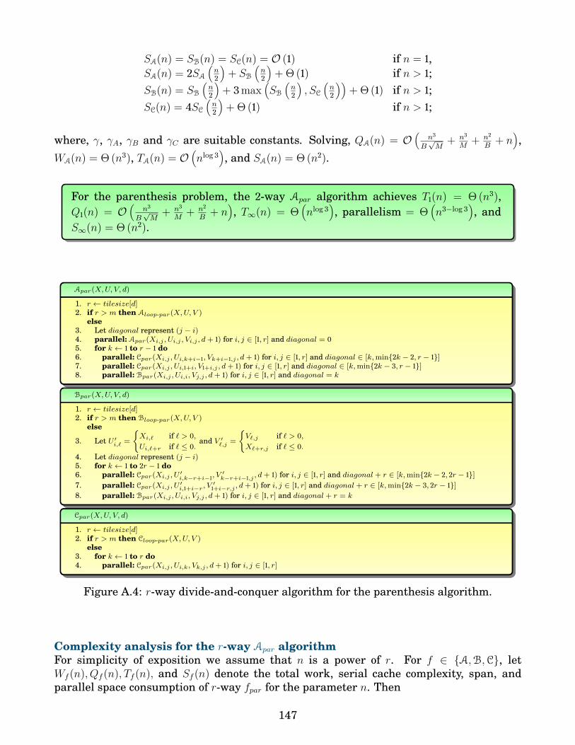
SA(n) = SB(n) = SC(n) = O (1) if n = 1,SA(n) = 2SA

(n2

)+ SB

(n2

)+ Θ (1) if n > 1;

SB(n) = SB

(n2

)+ 3max

(SB

(n2

), SC

(n2

))+ Θ (1) if n > 1;

SC(n) = 4SC

(n2

)+ Θ (1) if n > 1;

where, γ, γA, γB and γC are suitable constants. Solving, QA(n) = O(

n3

B√M

+ n3

M+ n2

B+ n

),

WA(n) = Θ (n3), TA(n) = O(nlog 3

), and SA(n) = Θ (n2).

For the parenthesis problem, the 2-way Apar algorithm achieves T1(n) = Θ (n3),Q1(n) = O

(n3

B√M

+ n3

M+ n2

B+ n

), T∞(n) = Θ

(nlog 3

), parallelism = Θ

(n3−log 3

), and

S∞(n) = Θ (n2).

Apar(X,U, V, d)

1. r ← tilesize[d]2. if r > m then Aloop-par(X,U, V )

else3. Let diagonal represent (j − i)4. parallel: Apar(Xi,j , Ui,j , Vi,j , d+ 1) for i, j ∈ [1, r] and diagonal = 05. for k ← 1 to r − 1 do6. parallel: Cpar(Xi,j , Ui,k+i−1, Vk+i−1,j , d+ 1) for i, j ∈ [1, r] and diagonal ∈ [k,min2k − 2, r − 1]7. parallel: Cpar(Xi,j , Ui,1+i, V1+i,j , d+ 1) for i, j ∈ [1, r] and diagonal ∈ [k,min2k − 3, r − 1]8. parallel: Bpar(Xi,j , Ui,i, Vj,j , d+ 1) for i, j ∈ [1, r] and diagonal = k

Bpar(X,U, V, d)

1. r ← tilesize[d]2. if r > m then Bloop-par(X,U, V )

else

3. Let U ′i,` =Xi,` if ` > 0,Ui,`+r if ` ≤ 0.

and V ′`,j =V`,j if ` > 0,X`+r,j if ` ≤ 0.

4. Let diagonal represent (j − i)5. for k ← 1 to 2r − 1 do6. parallel: Cpar(Xi,j , U

′i,k−r+i−1, V

′k−r+i−1,j , d+ 1) for i, j ∈ [1, r] and diagonal + r ∈ [k,min2k − 2, 2r − 1]

7. parallel: Cpar(Xi,j , U′i,1+i−r, V

′1+i−r,j , d+ 1) for i, j ∈ [1, r] and diagonal + r ∈ [k,min2k − 3, 2r − 1]

8. parallel: Bpar(Xi,j , Ui,i, Vj,j , d+ 1) for i, j ∈ [1, r] and diagonal + r = k

Cpar(X,U, V, d)

1. r ← tilesize[d]2. if r > m then Cloop-par(X,U, V )

else3. for k ← 1 to r do4. parallel: Cpar(Xi,j , Ui,k, Vk,j , d+ 1) for i, j ∈ [1, r]

Figure A.4: r-way divide-and-conquer algorithm for the parenthesis algorithm.

Complexity analysis for the r-way Apar algorithmFor simplicity of exposition we assume that n is a power of r. For f ∈ A,B,C, letWf (n), Qf (n), Tf (n), and Sf (n) denote the total work, serial cache complexity, span, andparallel space consumption of r-way fpar for the parameter n. Then

147

WA(n) = WB(n) = WC(n) = Θ (1) if n = 1,WA(n) = rWA

(nr

)+ r(r−1)

2 WB

(nr

)+ r(r−1)(r−2)

6 WC

(nr

)+ Θ (1) if n > 1;

WB(n) = r2WB

(nr

)+ r2(r − 1)WC

(nr

)+ Θ (1) if n > 1;

WC(n) = r3WC

(nr

)+ Θ (1) if n > 1;

QA(n) = QB(n) = QC(n) = O(n2

B+ 1

)if n2 ≤ γM ,

QA(n) = rQA

(nr

)+ r(r−1)

2 QB

(nr

)+ r(r−1)(r−2)

6 QC

(nr

)+ Θ (1) if n2 > γAM ;

QB(n) = r2QB

(nr

)+ r2(r − 1)QC

(nr

)+ Θ (1) if n2 > γBM ;

QC(n) = r3QC

(nr

)+ Θ (1) if n2 > γCM ;

TA(n) = TB(n) = TC(n) = O (1) if n = 1,TA(n) = TA

(nr

)+ TB

(nr

)+ (r−2)(r−1)

2 TC(nr

)+ Θ (1) if n > 1;

TB(n) = (2r − 1)(TB(nr

)+ (r − 1)TC

(nr

))+ Θ (1) if n > 1;

TC(n) = rTC(nr

)+ Θ (1) if n > 1;

where, γ, γA, γB and γC are suitable constants.

The serial cache complexity is computed as below.

QC(n) = r3QC

(n

r

)+ c = r3

(r3QC

(n

r2

)+ c

)+ c = (r3)2QC

(n

r2

)+ c

((r3)1 + 1

)= (r3)kQC

(n

rk

)+ c

((r3)k−1 + · · ·+ 1

) (say

(n

rk

)2≤ γM

)

= cr3k((

n

rk

)2 1B

+ 1)

+ c((r3)k−1 + · · ·+ 1

)= crk

n2

B+ c

((r3)k + · · ·+ 1

)= crk

n2

B+ cr3k

Let (n/rk)2 ≤ γM . This implies (n/rk−1)2 > γM or in other words rk−1 < n/√γM . Substi-

tuting the value of rk−1 in the above equation we have

QC(n) = crk−1rn2

B+ cr3k−3r3 ≤ cr

n3

B√M

+ cr3n3

M√M

= O(

n3r

B√M

+ n3r3

M√M

)

= O

n3

B⌈ √

Mr

⌉ + n3⌈ √Mr

⌉3

148

We now consider the cache complexity of the Bpar function using the complexity of Cpar.

QB(n) ≤ r2QB

(n

r

)+ r2(r − 1)QC

(n

r

)+ c

= r2(r2QB

(n

r2

)+ r2(r − 1)QC

(n

r2

)+ c

)+ r2(r − 1)QC

(n

r

)+ c

= (r2)2QB

(n

r2

)+ (r2)2(r − 1)QC

(n

r2

)+ cr2 + r2(r − 1)QC

(n

r

)+ c

= (r2)kQB

(n

rk

)+ r2(r − 1)

((r2)k−1QC

(n

rk

)+ · · ·+QC

(n

r

))+ c

((r2)k−1 + · · ·+ 1

)≤ cr2k

((n

rk

)2 1B

+ 1)

+ r2(r − 1)k∑i=1

((r2)i−1QC

(n

ri

))+ c

((r2)k−1 + · · ·+ 1

)

= cn2

B+ cr2(r − 1)

k∑i=1

((r2)i−1

((n

ri

)3 r

B√M

+(n

ri

)3 r3

M√M

))+ cr2k

= cn2

B+ c

n3

B√Mr(r − 1)

k∑i=1

1ri

+ cn3

M√Mr3(r − 1)

k∑i=1

1ri

+ cr2k

= cn2

B+ c

n3

B√Mr(r − 1) rk − 1

rk(r − 1) + cn3

M√Mr3(r − 1) rk − 1

rk(r − 1) + cr2k

= cn2

B+ c

n3

B√M

(r − 1

rk−1

)+ c

n3

M√M

(r3 − r2

rk−1

)+ cr2k−2r2

Substituting the upper bound of rk−1, we have

QB(n) ≤ cn2

B+ c

n3

B√M

(r −√M

n

)+ c

n3

M√M

(r3 − r2

√M

n

)+ cr2k−2r2

≤ cn2

B+ c

n3r

B√M

+ cn3r3

M√M

+ cn2r2

M= O

(n3r

B√M

+ n3r3

M√M

+ n2

B+ n2r2

M

)

= O

n3

B⌈ √

Mr

⌉ + n3⌈ √Mr

⌉3 + n2

B+ n2⌈ √

Mr

⌉2

With the cache complexity of Bpar and Cpar functions, we can easily find the cache com-

149

plexity of the A function.

QA(n) ≤ rQA

(n

r

)+ r(r − 1)

2QB

(n

r

)+ r(r − 1)(r − 2)

6QC

(n

r

)+ c

= r

(rQA

(n

r2

)+ r(r − 1)

2QB

(n

r2

)+ r(r − 1)(r − 2)

6QC

(n

r2

)+ c

)

+ r(r − 1)2

QB

(n

r

)+ r(r − 1)(r − 2)

6QC

(n

r

)+ c

= r2QA

(n

r2

)+ r(r − 1)

2

(rQB

(n

r2

)+QB

(n

r

))+ r(r − 1)(r − 2)

6

(rQC

(n

r2

)+QC

(n

r

))+ c(r + 1)

= rkQA

(n

rk

)+ r(r − 1)

2

(rk−1QB

(n

rk

)+ · · ·+QB

(n

r

))+ r(r − 1)(r − 2)

6

(rk−1QC

(n

rk

)+ · · ·+QC

(n

r

))+ c(rk−1 + · · ·+ 1)

= crk((

n

rk

)2 1B

+ 1)

+ r(r − 1)2

k∑i=1

ri−1QB

(n

ri

)

+ r(r − 1)(r − 2)6

k∑i=1

ri−1QC

(n

ri

)+ c(rk−1 + · · ·+ 1)

= c1rkn2

B+ c

r(r − 1)2

k∑i=1

(ri−1

((n

ri

)3 r

B√M

+(n

ri

)3 r3

M√M

+(n

ri

)2 1B

+(n

ri

)2 r2

M

))

+ cr(r − 1)(r − 2)

6

k∑i=1

(ri−1

((n

ri

)3 r

B√M

+(n

ri

)3 r3

M√M

))+ crk

= c1rkn2

B+ c

r(r − 1)2

n3

B√M

k∑i=1

1r2i

+ cr3(r − 1)

2n3

M√M

k∑i=1

1r2i

+ c(r − 1)

2n2

B

k∑i=1

1ri

+ cr2(r − 1)

2n2

M

k∑i=1

1ri

+ cr(r − 1)(r − 2)

6n3

B√M

k∑i=1

1r2i

+ cr3(r − 1)(r − 2)

6n3

M√M

k∑i=1

1r2i

+ crk

After substituting∑ki=1(1/ri) = (rk − 1)/(rk(r − 1)) and

∑ki=1(1/r2i) = (r2k − 1)/(r2k(r2 − 1))

in the equation above and simplifying, we have

QA(n) ≤ c1

rrk−1n2

B+ c

2r

r + 1

(1− 1

r2r2k−2

)n3

B√M

+ c

2r3

r + 1

(1− 1

r2r2k−2

)n3

M√M

+ c

2

(1− 1

rrk−1

)n2

B+ c

2

(r2 − r

rk−1

)n2

M+ c

6r(r − 2)r + 1

(1− 1

r2r2k−2

)n3

B√M

+ c

6r3(r − 2)r + 1

(1− 1

r2r2k−2

)n3

M√M

+ crrk−1

150

Substituting the value of rk−1, we get

QA(n) ≤ c

√M

nr

n2

B+ c

2r

r + 1

(1− M

n2r2

)n3

B√M

+ c

2r3

r + 1

(1− M

n2r2

)n3

M√M

+ c

2

(1−√M

nr

)n2

B+ c

2

(r2 −

√Mr

n

)n2

M+ c

6r(r − 2)r + 1

(1− M

n2r2

)n3

B√M

+ c

6r3(r − 2)r + 1

(1− M

n2r2

)n3

M√M

+ cnr√M

≤ cn√M

rB+ c

2n3

B√M

+ c

2n3r2

M√M

+ c

2n2

B+ c

2n2r2

M+ c

6n3r

B√M

+ c

6n3r3

M√M

+ cnr√M

= O(

n3r

B√M

+ n3r3

M√M

+ n2

B+ n2r2

M+ n√M

rB+ nr√

M

)

= O

n3

B⌈ √

Mr

⌉ + n3⌈ √Mr

⌉3 + n2

B+ n2⌈ √

Mr

⌉2 + n

B

⌈ √M

r

⌉+ n⌈ √

Mr

⌉

We now show the analysis for the span of the r-way divide-and-conquer algorithm. Sim-ilar to the previous analysis we assume (n/rk) = 1, or rk = n or k = logr n.

TC(n) = rTC

(n

r

)+ c = r

(rTC

(n

r2

)+ c

)+ c = r2TC

(n

r2

)+ c(r + 1)

= rkTC

(n

rk

)+ c

(rk−1 + · · ·+ 1

)= crk(1) + c

(rk−1 + · · ·+ 1

)≤ c′rk = Θ (n)

TB(n) = (2r − 1)TB(n

r

)+ (r − 1)(2r − 1)TC

(n

r

)+ c

= (2r − 1)(

(2r − 1)TB(n

r2

)+ (r − 1)(2r − 1)TC

(n

r2

)+ c

)+ (r − 1)(2r − 1)TC

(n

r

)+ c

= (2r − 1)2TB(n

r2

)+ (r − 1)(2r − 1)

((2r − 1)TC

(n

r2

)+ TC

(n

r

))+ c ((2r − 1) + 1)

= (2r − 1)kTB(n

rk

)+ (r − 1)(2r − 1)

((2r − 1)k−1TC

(n

rk

)+ · · ·+ TC

(n

r

))+ c

((2r − 1)k−1 + · · ·+ 1

)≤ (2r − 1)k(c) + (r − 1)(2r − 1)

k∑i=1

(2r − 1)i−1TC(n

ri

)+ c

((2r − 1)k−1 + · · ·+ 1

)

≤ (2r − 1)k(c) + c(r − 1)(2r − 1)k∑i=1

(2r − 1)i−1 nri

+ c((2r − 1)k−1 + · · ·+ 1

)

= c(r − 1)(2r − 1)

(2− 1

r

)k− 1

r − 1

+ c′(2r − 1)k = c(2r − 1)((

2− 1r

)k− 1

)+ c′(2r − 1)k

151

Substituting the value of k = logr n, we have

TB(n) ≤ c(2r − 1)((

2− 1r

)logr n

− 1)

+ c′(2r − 1)logr n

= c(2r − 1)(nlogr (2− 1

r ) − 1)

+ c′nlogr(2r−1) = Θ(rnlogr (2− 1

r ) + nlogr(2r−1))

TA(n) = TA

(n

r

)+ TB

(n

r

)+ (r − 2)(r − 1)

2TC

(n

r

)+ c

=(TA

(n

r2

)+ TB

(n

r2

)+ (r − 2)(r − 1)

2TC

(n

r2

)+ c

)+ TB

(n

r

)+ (r − 2)(r − 1)

2TC

(n

r

)+ c

= TA

(n

r2

)+ TB

(n

r2

)+ TB

(n

r

)+ (r − 2)(r − 1)

2

(TC

(n

r2

)+ TC

(n

r

))+ 2c

= TA

(n

rk

)+(TB

(n

rk

)+ · · ·+ TB

(n

r

))+ (r − 2)(r − 1)

2

(TC

(n

rk

)+ · · ·+ TC

(n

r

))+ kc

≤ c+k∑i=1

TB

(n

ri

)+ (r − 2)(r − 1)

2

k∑i=1

TC

(n

ri

)+ kc

≤ ck∑i=1

r ( nri

)logr (2− 1r )

+(n

ri

)logr(2r−1)+ c

(r − 2)(r − 1)2

k∑i=1

n

ri+ kc

≤ crnlogr (2− 1r )

k∑i=1

1(rlogr (2− 1

r ))i + cnlogr(2r−1)

k∑i=1

1(rlogr(2r−1))i

+ cn(r − 2)(r − 1)

2

k∑i=1

1ri

+ kc

≤ crnlogr (2− 1r )

k∑i=1

1(2− 1

r

)i + cnlogr(2r−1)k∑i=1

1(2r − 1)i

+ cn(r − 2)(r − 1)

2

k∑i=1

1ri

+ kc

≤ cnlogr (2− 1r ) r2

r − 1

1− 1(2− 1

r

)k+ cnlogr(2r−1) 1

2(r − 1)

(1− 1

(2r − 1)k

)+ cn

(r − 2)2

(1− 1

rk

)+ kc

Substituting the value of k = logr n and simplifying we have

TA(n) = O(rnlogr(2− 1

r ) + nlogr(2r−1)

r+ nr

)

For the parenthesis problem, the r-way Apar algorithm achieves T1(n) =

Θ (n3), Q1(n) = O

n3

B

⌈√

Mr

⌉ + n3⌈√

Mr

⌉3 + n2

B+ n2⌈

√Mr

⌉2 + nB

⌈ √Mr

⌉+ n⌈

√Mr

⌉, T∞(n) =

Θ(rnlogr(2− 1

r ) + nlogr(2r−1)

r+ nr

), parallelism = T1(n)

T∞(n) , and S∞(n) = Θ (n2).

A.3 Floyd-Warshall’s all-pairs shortest pathAn algebraic structure known as a closed semiring [Aho et al., 1974] serves as a generalframework for solving path problems in directed graphs. In [Aho et al., 1974], an algorithm

152

is given for finding the set of all paths between each pair of vertices in a directed graph.Both Floyd-Warshall’s algorithm for finding all-pairs shortest paths [Floyd, 1962] and War-shall’s algorithm for finding transitive closures [Warshall, 1962] are instantiations of thisalgorithm.

Consider a directed graph G = (V,E), where V = v1, v2, . . . , vn, and each edge (vi, vj) islabeled by an element `(vi, vj) of some closed semiring (S,⊕,, 0, 1). If (vi, vj) < E, `(vi, vj)is assumed to have a value 0. The path-cost of a path is defined as the product () of thelabels of the edges in the path, taken in order. The path-cost of a zero length path is 1. Foreach pair vi, vj ∈ V , d[i, j] is defined to be the sum of the path-costs of all paths going fromvi to vj. By convention, the sum over an empty set of paths is 0. Even if there are infinitelymany paths between vi and vj (due to presence of cycles), d[i, j] will still be well-defined dueto the properties of a closed semiring.

For i, j ∈ [1, n] and k ∈ [0, n], let D[i, j, k] denote cost of the smallest cost path from vito vj with no intermediate vertex higher than vk. Then d[i, j] = D[i, j, n]. The followingrecurrence computes all D[i, j, k].

D[i, j, k] =

1 if k = 0 and i = j,l(vi, vj) if k = 0 and i , j,D[i, j, k − 1]⊕ (D[i, k, k − 1]D[k, j, k − 1]) if k > 0.

(A.4)

The dependency structure of the DP is shown in Figure A.5. Floyd-Warshall’s APSPperforms computations over a particular closed semiring (R,min,+,+∞, 0).

A serial and a parallel iterative algorithm for computing the path costs are given inFigure A.5. The structure of the three loops seems similar to the matrix multiplicationalgorithm but there are differences. In matrix multiplication, the i-j-k loops can be orderedin any of the 3! = 6 ways. However, in the computation of path costs, the k-loop must alwaysbe the outermost loop.

Figures A.5 and A.6 show a divide-and-conquer implementation [Chowdhury and Ra-machandran, 2010] of the Floyd-Warshall’s APSP algorithm. The implementation consistsof four recursive divide-and-conquer functions. The number of times Aloop−FW , Bloop−FW ,Cloop−FW , and Dloop−FW will be called are Θ (n) ,Θ (n2) ,Θ (n2), and Θ (n3) respectively. Hence,function DFW is dominating.

Complexity analysis for the PAR-LOOP-PATH-COSTS algorithmFor f ∈ PAR-LOOP-PATH-COSTS, let Qf (n) and Tf (n) denote the serial cache complexity,and span of fFW on a matrix of size n × n. Wf (n) is Θ (n3). Qf (n) is computed as Qf (n) =Θ(n · n ·

(nB

+ 1))

= Θ(n3

B+ n2

). The span is Tf (n) = Θ (n · (log n+ (log n+ Θ (1)))) = Θ (n log n).

The properties of the given semiring implies that d[i, j] for all pairs of vertices vi, vj ∈ Vuses only Θ (n2) space as shown in Figure A.5.

For the Floyd-Warshall’s all-pairs shortest path algorithm, the PAR-LOOP-PATH-COSTS implementation achieves T1(n) = Θ (n3), Q1(n) = Θ

(n3

B+ n2

), T∞(n) =

Θ (n log n), parallelism = Θ(

n2

logn

), and S∞(n) = Θ (n2).

Complexity analysis for the 2-way AFW algorithmFor f ∈ A,B,C,D, let Qf (n) and Tf (n) denote the serial cache complexity, and span offFW on a matrix of size n× n. Then

153

LOOP-PATH-COSTS(D)

1. for i← 1 to n do2. for j ← 1 to n do3. d[i, j]← D[i, j, 0]4. for k ← 1 to n do5. for i← 1 to n do6. for j ← 1 to n do7. d[i, j]← d[i, j]⊕ (d[i, k] d[k, j])

PAR-LOOP-PATH-COSTS(D)

1. parallel for i← 1 to n do2. parallel for j ← 1 to n do3. d[i, j]← D[i, j, 0]4. for k ← 1 to n do5. parallel for i← 1 to n do6. parallel for j ← 1 to n do7. d[i, j]← d[i, j]⊕ (d[i, k] d[k, j])

AF W (X)

1. if X is a small matrix then Aloop-F W (X)else

2. AF W (X11)3. par: BF W (X12, X11), CF W (X21, X11)4. DF W (X22, X21, X12)5. AF W (X22)6. par: BF W (X21, X22), CF W (X12, X22)7. DF W (X11, X12, X21)

BF W (X,U)

1. if X is a small matrix then Bloop-F W (X,U)else

2. par: BF W (X11, U11), BF W (X12, U11)3. par: DF W (X21, U21, X11), DF W (X22, U21, X12)4. par: BF W (X21, U22), BF W (X22, U22)5. par: DF W (X11, U12, X21), DF W (X12, U12, X22)

CF W (X,V )

1. if X is a small matrix then Cloop-F W (X,V )else

2. par: CF W (X11, V11), CF W (X21, V11)3. par: DF W (X12, X11, V12), DF W (X22, X21, V12)4. par: CF W (X12, V22), CF W (X22, V22)5. par: DF W (X11, X12, V21), DF W (X21, X22, V21)

DF W (X,U, V )

1. if X is a small matrix then Dloop-F W (X,U, V )else

2. par: DF W (X11, U11, V11), DF W (X12, U11, V12),DF W (X21, U21, V11), DF W (X22, U21, V12)

3. par: DF W (X11, U12, V21), DF W (X12, U12, V22),DF W (X21, U22, V21), DF W (X22, U22, V22)

Figure A.5: Top left: Serial and parallel iterative algorithms to compute path costs over aclosed semiring (S,⊕,, 0, 1). Top right: Dependency structure for Floyd-Warshall’s APSPalgorithm. Bottom: Divide-and-conquer algorithm.

QA(n) = QB(n) = QC(n) = QD(n) = O(n2

B+ n

)if n2 ≤ γM ,

QA(n) = 2(QA

(n2

)+QB

(n2

)+QC

(n2

)+QD

(n2

))+ Θ (1) if n2 > γAM ;

QB(n) = 4(QB

(n2

)+QD

(n2

))+ Θ (1) if n2 > γBM ;

QC(n) = 4(QC

(n2

)+QD

(n2

))+ Θ (1) if n2 > γCM ;

QD(n) = 8QD

(n2

)+ Θ (1) if n2 > γDM ;

TA(n) = TB(n) = TC(n) = TD(n) = O (1) if n = 1,TA(n) = 2

(TA(n2

)+ max TB

(n2

), TC

(n2

)+ TD

(n2

))+ Θ (1) if n > 1;

TB(n) = 2(TB(n2

)+ TD

(n2

))+ Θ (1) if n > 1;

TC(n) = 2(TC(n2

)+ TD

(n2

))+ Θ (1) if n > 1;

TD(n) = 2TD(n2

)+ Θ (1) if n > 1;

154

Figure A.6: A divide-and-conquer algorithm AFW for solving the Floyd-Warshall’s all-pairsshortest path problem.

155

where, γ, γA, γB, γC and γD are suitable constants. Solving, QA(n) = O(

n3

B√M

+ n3

M+ n2

B+ n

)and TA(n) = O

(n log2 n

).

For the Floyd-Warshall’s all-pairs shortest path algorithm, the AFW implementa-tion achieves T1(n) = Θ (n3), Q1(n) = O

(n3

B√M

+ n3

M+ n2

B+ n

), T∞(n) = Θ

(n log2 n

),

parallelism = Θ(

n2

log2 n

), and S∞(n) = Θ (n2).

AF W (X,U, V, d)

1. r ← tilesize[d]2. if r > m then Aloop-F W (X,U, V )

else3. for k ← 1 to r do4. AF W (Xkk, Ukk, Vkk, d+ 1)5. parallel:

for j ← 1 to r doif j , k then BF W (Xkj , Ukk, Vkj , d+ 1)

for i← 1 to r doif i , k then CF W (Xik, Uik, Vkk, d+ 1)

6. parallel for i← 1 to r do7. parallel for j ← 1 to r do8. if i , k and j , k then9. DF W (Xij , Uik, Vkj , d+ 1)

DF W (X,U, V )

1. r ← tilesize[d]2. if r > m then Dloop-F W (X,U, V )

else3. for k ← 1 to r do4. parallel for i← 1 to r do5. parallel for j ← 1 to r do6. DF W (Xij , Uik, Vkj , d+ 1)

BF W (X,U, V, d)

1. r ← tilesize[d]2. if r > m then Bloop-F W (X,U, V )

else3. for k ← 1 to r do4. parallel for j ← 1 to r do

BF W (Xkj , Ukk, Vkj , d+ 1)5. parallel for i← 1 to r do6. parallel for j ← 1 to r do7. if i , k then DF W (Xij , Uik, Vkj , d+ 1)

CF W (X,U, V, d)

1. r ← tilesize[d]2. if r > m then Cloop-F W (X,U, V )

else3. for k ← 1 to r do4. parallel for i← 1 to r do

CF W (Xik, Uik, Vkk, d+ 1)5. parallel for i← 1 to r do6. parallel for j ← 1 to r do7. if j , k then DF W (Xij , Uik, Vkj , d+ 1)

Figure A.7: r-way divide-and-conquer algorithm for Floyd-Warshall algorithm.

Complexity analysis for the r-way AFW algorithmThe r-way divide-and-conquer for Floyd-Warshall algorithm is given in Figure A.7. For sim-plicity of exposition we assume that n is a power of r. For f ∈ A,B,C,D, letWf (n), Qf (n), Tf (n),and Sf (n) denote the total work, serial cache complexity, span, and parallel space consump-tion of r-way fFW for the parameter n. Then

WA(n) = WB(n) = WC(n) = WD(n) = Θ (1) if n = 1,WA(n) = rWA

(nr

)+ r(r − 1)

(WB

(nr

)+WC

(nr

))+ r(r − 1)2WD

(nr

)+ Θ (1) if n > 1;

WB(n) = r2WB

(nr

)+ r2(r − 1)WD

(nr

)+ Θ (1) if n > 1;

WC(n) = r2WC

(nr

)+ r2(r − 1)WD

(nr

)+ Θ (1) if n > 1;

WD(n) = r3WD

(nr

)+ Θ (1) if n > 1;

156

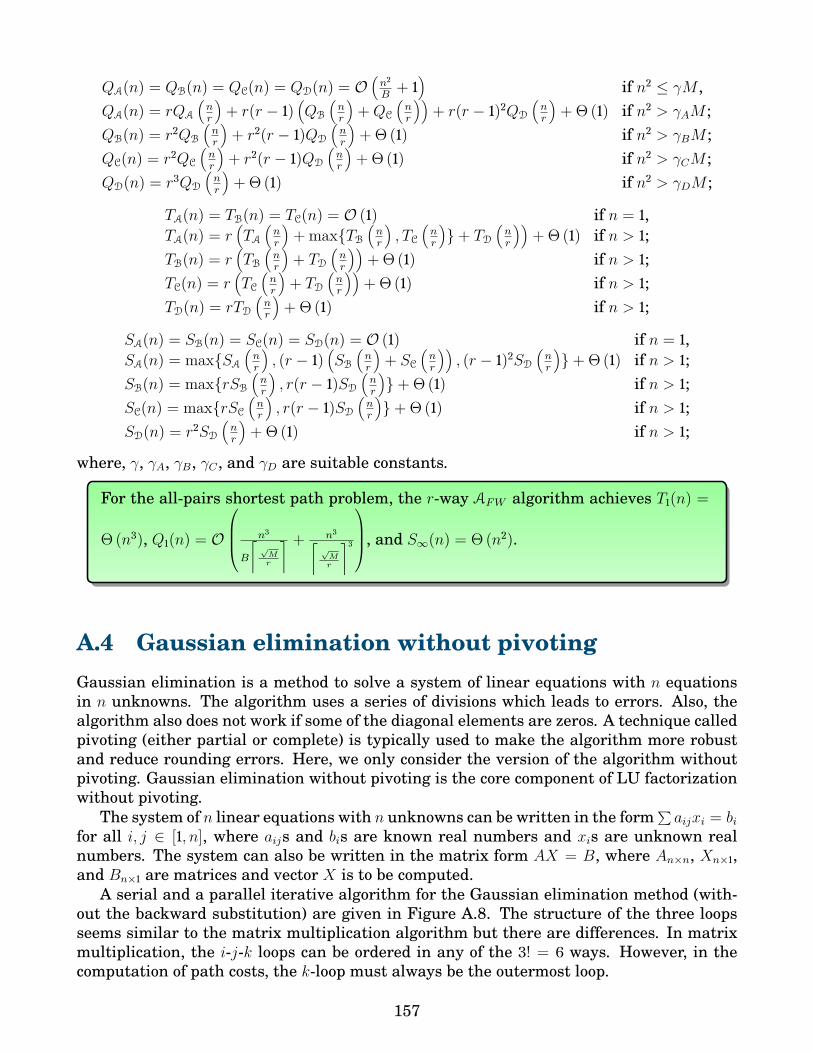
QA(n) = QB(n) = QC(n) = QD(n) = O(n2

B+ 1

)if n2 ≤ γM ,

QA(n) = rQA

(nr

)+ r(r − 1)

(QB

(nr

)+QC

(nr

))+ r(r − 1)2QD

(nr

)+ Θ (1) if n2 > γAM ;

QB(n) = r2QB

(nr

)+ r2(r − 1)QD

(nr

)+ Θ (1) if n2 > γBM ;

QC(n) = r2QC

(nr

)+ r2(r − 1)QD

(nr

)+ Θ (1) if n2 > γCM ;

QD(n) = r3QD

(nr

)+ Θ (1) if n2 > γDM ;

TA(n) = TB(n) = TC(n) = O (1) if n = 1,TA(n) = r

(TA(nr

)+ maxTB

(nr

), TC

(nr

)+ TD

(nr

))+ Θ (1) if n > 1;

TB(n) = r(TB(nr

)+ TD

(nr

))+ Θ (1) if n > 1;

TC(n) = r(TC(nr

)+ TD

(nr

))+ Θ (1) if n > 1;

TD(n) = rTD(nr

)+ Θ (1) if n > 1;

SA(n) = SB(n) = SC(n) = SD(n) = O (1) if n = 1,SA(n) = maxSA

(nr

), (r − 1)

(SB

(nr

)+ SC

(nr

)), (r − 1)2SD

(nr

)+ Θ (1) if n > 1;

SB(n) = maxrSB

(nr

), r(r − 1)SD

(nr

)+ Θ (1) if n > 1;

SC(n) = maxrSC

(nr

), r(r − 1)SD

(nr

)+ Θ (1) if n > 1;

SD(n) = r2SD

(nr

)+ Θ (1) if n > 1;

where, γ, γA, γB, γC , and γD are suitable constants.

For the all-pairs shortest path problem, the r-way AFW algorithm achieves T1(n) =

Θ (n3), Q1(n) = O

n3

B

⌈√

Mr

⌉ + n3⌈√

Mr

⌉3

, and S∞(n) = Θ (n2).

A.4 Gaussian elimination without pivotingGaussian elimination is a method to solve a system of linear equations with n equationsin n unknowns. The algorithm uses a series of divisions which leads to errors. Also, thealgorithm also does not work if some of the diagonal elements are zeros. A technique calledpivoting (either partial or complete) is typically used to make the algorithm more robustand reduce rounding errors. Here, we only consider the version of the algorithm withoutpivoting. Gaussian elimination without pivoting is the core component of LU factorizationwithout pivoting.

The system of n linear equations with n unknowns can be written in the form∑aijxi = bi

for all i, j ∈ [1, n], where aijs and bis are known real numbers and xis are unknown realnumbers. The system can also be written in the matrix form AX = B, where An×n, Xn×1,and Bn×1 are matrices and vector X is to be computed.

A serial and a parallel iterative algorithm for the Gaussian elimination method (with-out the backward substitution) are given in Figure A.8. The structure of the three loopsseems similar to the matrix multiplication algorithm but there are differences. In matrixmultiplication, the i-j-k loops can be ordered in any of the 3! = 6 ways. However, in thecomputation of path costs, the k-loop must always be the outermost loop.

157

LOOP-GAUSSIAN-ELIMINATION(D)

1. for k ← 1 to n− 1 do2. for i← k + 1 to n do3. for j ← k to n do4. d[i, j]← d[i, j]− (d[i, k]× d[k, j]) /d[k, k]

PAR-GAUSSIAN-ELIMINATION(D)

1. for k ← 1 to n− 1 do2. parallel for i← k + 1 to n do3. parallel for j ← k to n do4. d[i, j]← d[i, j]− (d[i, k]× d[k, j]) /d[k, k]

AGE(X)

1. if X is a small matrix then Aloop-GE(X)else

2. AGE(X11)3. par: BGE(X12, X11), CGE(X21, X11)4. DGE(X22, X21, X12)5. AGE(X22)

BGE(X,U)

1. if X is a small matrix then Bloop-GE(X,U)else

2. par: BGE(X11, U11), BGE(X12, U11)3. par: DGE(X21, U21, X11), DGE(X22, U21, X12)4. par: BGE(X21, U22), BGE(X22, U22)

CGE(X,V )

1. if X is a small matrix then Cloop-GE(X,V )else

2. par: CGE(X11, V11), CGE(X21, V11)3. par: DGE(X12, X11, V12), DGE(X22, X21, V12)4. par: CGE(X12, V22), CGE(X22, V22)

DGE(X,U, V )

1. if X is a small matrix then Dloop-GE(X,U, V )else

2. par: DGE(X11, U11, V11), DGE(X12, U11, V12),DGE(X21, U21, V11), DGE(X22, U21, V12)

3. par: DGE(X11, U12, V21), DGE(X12, U12, V22),DGE(X21, U22, V21), DGE(X22, U22, V22)

Figure A.8: Top left: Serial and parallel iterative algorithms for Gaussian elimination.Top right: Dependency structure for Gaussian elimination. Bottom: Divide-and-conqueralgorithm.

Figures A.8 and A.9 show a divide-and-conquer implementation of the Gaussian elimi-nation algorithm. The implementation consists of four recursive divide-and-conquer func-tions. The number of times Aloop−GE, Bloop−GE, Cloop−GE, and Dloop−GE will be called areΘ (n) ,Θ (n2) ,Θ (n2), and Θ (n3) respectively. Hence, function DGE is dominating.

Complexity analysis for the PAR-GAUSSIAN-ELIMINATION algorithmFor f ∈ PAR-GAUSSIAN-ELIMINATION, let Qf (n) and Tf (n) denote the serial cache com-plexity, and span of fFW on a matrix of size n × n. Wf (n) is Θ (n3). Qf (n) is computed asQf (n) = Θ

(n · n ·

(nB

+ 1))

= Θ(n3

B+ n2

). The span is Tf (n) = Θ (n · (log n+ (log n+ Θ (1)))) =

Θ (n log n). The properties of the given semiring implies that d[i, j] for all pairs of verticesvi, vj ∈ V uses only Θ (n2) space as shown in Figure A.5.

For the Gaussian elimination algorithm, the PAR-GAUSSIAN-ELIMINATION imple-mentation achieves T1(n) = Θ (n3), Q1(n) = Θ

(n3

B+ n2

), T∞(n) = Θ (n log n), paral-

lelism = Θ(

n2

logn

), and S∞(n) = Θ (n2).

Complexity analysis for the 2-way AGE algorithmFor f ∈ A,B,C,D, let Qf (n) and Tf (n) denote the serial cache complexity, and span of fGEon a matrix of size n× n. Then

158

Figure A.9: A divide-and-conquer algorithm AGE for Gaussian elimination.

QA(n) = QB(n) = QC(n) = QD(n) = O(n2

B+ n

)if n2 ≤ γM ,

QA(n) = 2QA

(n2

)+QB

(n2

)+QC

(n2

)+QD

(n2

)+ Θ (1) if n2 > γAM ;

QB(n) = 4QB

(n2

)+ 2QD

(n2

)+ Θ (1) if n2 > γBM ;

QC(n) = 4QC

(n2

)+ 2QD

(n2

)+ Θ (1) if n2 > γCM ;

QD(n) = 8QD

(n2

)+ Θ (1) if n2 > γDM ;

159

TA(n) = TB(n) = TC(n) = TD(n) = O (1) if n = 1,TA(n) = 2TA

(n2

)+ max TB

(n2

), TC

(n2

)+ TD

(n2

)+ Θ (1) if n > 1;

TB(n) = 2TB(n2

)+ TD

(n2

)+ Θ (1) if n > 1;

TC(n) = 2TC(n2

)+ TD

(n2

)+ Θ (1) if n > 1;

TD(n) = 2TD(n2

)+ Θ (1) if n > 1;


n3

B√M

+ n3

M+ n2

B+ n

)and TA(n) = O

(n log2 n

).

For the Gaussian elimination algorithm, the AGE implementation achieves T1(n) =Θ (n3), Q1(n) = O

(n3

B√M

+ n3

M+ n2

B+ n

), T∞(n) = Θ

(n log2 n

), parallelism = Θ

(n2

log2 n

),

and S∞(n) = Θ (n2).

AGE(X,U, V,W, d)

1. r ← tilesize[d]2. if r > m then Aloop-GE(X,U, V,W )

else3. for k ← 1 to r do4. AGE(Xkk, Ukk, Vkk,Wk, d+ 1)5. parallel:

for j ← k + 1 to r doBGE(Xkj , Ukk, Vkj ,Wk, d+ 1)

for i← k + 1 to r doCGE(Xik, Uik, Vkk,Wk, d+ 1)

6. parallel for i← k + 1 to r do7. parallel for j ← k + 1 to r do8. DGE(Xij , Uik, Vkj ,Wk, d+ 1)

DGE(X,U, V,W, d)

1. r ← tilesize[d]2. if r > m then Dloop-GE(X,U, V,W )

else3. for k ← 1 to r do4. parallel for i← 1 to r do5. parallel for j ← 1 to r do6. DGE(Xij , Uik, Vkj ,Wk, d+ 1)

BGE(X,U, V,W, d)

1. r ← tilesize[d]2. if r > m then Bloop-GE(X,U, V,W )

else3. for k ← 1 to r do4. parallel for j ← 1 to r do

BGE(Xkj , Ukk, Vkj ,Wk, d+ 1)5. parallel for i← k + 1 to r do6. parallel for j ← 1 to r do7. DGE(Xij , Uik, Vkj ,Wk, d+ 1)

CGE(X,U, V,W, d)

1. r ← tilesize[d]2. if r > m then Cloop-GE(X,U, V,W )

else3. for k ← 1 to r do4. parallel for i← 1 to r do

CGE(Xik, Uik, Vkk,Wk, d+ 1)5. parallel for i← 1 to r do6. parallel for j ← k + 1 to r do7. DGE(Xij , Uik, Vkj ,Wk, d+ 1)

Figure A.10: An r-way divide-and-conquer algorithm for Gaussian elimination.

Complexity analysis for the r-way AGE algorithmAn r-way divide-and-conquer algorithm for Gaussian elimination is given in Figure D.3.For simplicity of exposition we assume that n is a power of r. For f ∈ A,B,C,D, letWf (n), Qf (n), Tf (n), and Sf (n) denote the total work, serial cache complexity, span, andparallel space consumption of r-way fGE for the parameter n. Then

WA(n) = WB(n) = WC(n) = WD(n) = Θ (1) if n = 1,WA(n) = rWA

(nr

)+ r(r−1)

2

(WB

(nr

)+WC

(nr

))+ r(r−1)(2r−1)

6 WD

(nr

)+ Θ (1) if n > 1;

WB(n) = r2WB

(nr

)+ r2(r−1)

2 WD

(nr

)+ Θ (1) if n > 1;

WC(n) = r2WC

(nr

)+ r2(r−1)

2 WD

(nr

)+ Θ (1) if n > 1;

WD(n) = r3WD

(nr

)+ Θ (1) if n > 1;

160

QA(n) = QB(n) = QC(n) = QD(n) = O(n2

B+ 1

)if n2 ≤ γM ,

QA(n) = rQA

(nr

)+ r(r−1)

2

(QB

(nr

)+QC

(nr

))+ r(r−1)(2r−1)

6 QD

(nr

)+ Θ (1) if n2 > γAM ;

QB(n) = r2QB

(nr

)+ r2(r−1)

2 QD

(nr

)+ Θ (1) if n2 > γBM ;

QC(n) = r2QC

(nr

)+ r2(r−1)

2 QD

(nr

)+ Θ (1) if n2 > γCM ;

QD(n) = r3QD

(nr

)+ Θ (1) if n2 > γDM ;

TA(n) = TB(n) = TC(n) = O (1) if n = 1,TA(n) = rTA

(nr

)+ (r − 1) maxTB

(nr

), TC

(nr

)+ (r − 1)TD

(nr

)+ Θ (1) if n > 1;

TB(n) = rTB(nr

)+ (r − 1)TD

(nr

)+ Θ (1) if n > 1;

TC(n) = rTC(nr

)+ (r − 1)TD

(nr

)+ Θ (1) if n > 1;

TD(n) = rTD(nr

)+ Θ (1) if n > 1;

SA(n) = SB(n) = SC(n) = SD(n) = O (1) if n = 1,SA(n) = maxSA

(nr

), (r − 1)

(SB

(nr

)+ SC

(nr

)), (r − 1)2SD

(nr

)+ Θ (1) if n > 1;

SB(n) = maxrSB

(nr

), r(r − 1)SD

(nr

)+ Θ (1) if n > 1;

SC(n) = maxrSC

(nr

), r(r − 1)SD

(nr

)+ Θ (1) if n > 1;

SD(n) = r2SD

(nr

)+ Θ (1) if n > 1;

where, γ, γA, γB, γC , and γD are suitable constants.

For the Gaussian elimination algorithm, the r-way AGE algorithm achieves T1(n) =

Θ (n3), Q1(n) = O

n3

B

⌈√

Mr

⌉ + n3⌈√

Mr

⌉3

, and S∞(n) = Θ (n2).

A.5 Sequence alignment with gap penalty

The sequence alignment problem with gap penalty or often called the gap problem [Galiland Giancarlo, 1989, Galil and Park, 1994, Waterman et al., 1995] is a generalization ofthe edit distance problem that arises in molecular biology, geology, and speech recognition.When transforming a string X = x1x2 . . . xm into another string Y = y1y2 . . . yn, a sequenceof consecutive deletes corresponds to a gap in X, and a sequence of consecutive insertscorresponds to a gap in Y . In many applications the cost of such a gap is not necessarilyequal to the sum of the costs of each individual deletion (or insertion) in that gap. In orderto handle this general case two new cost functions w and w′ are defined, where w(p, q)(0 ≤ p < q ≤ m) is the cost of deleting xp+1 . . . xq from X, and w′(p, q) (0 ≤ p < q ≤ n) is thecost of inserting yp+1 . . . yq into X. The substitution function S(xi, yj) is the same as that ofthe standard edit distance problem.

Let G[i, j] denote the minimum cost of transforming Xi = x1x2 . . . xi into Yj = y1y2 . . . yj(where 0 ≤ i ≤ m and 0 ≤ j ≤ n) under this general setting. Then

161

G[i, j] =

0 if i = j = 0,w(0, j) if i = 0, 1 ≤ j ≤ n,w′(0, i) if j = 0, 1 ≤ i ≤ m,

min

G[i− 1, j − 1] + S(xi, yj),

min0≤q<j G[i, q] + w(q, j) ,min0≤p<i G[p, j] + w′(p, i)

if i, j > 0.(A.5)

Assuming m = n, this problem can be solved in Θ (n3) time using Θ (n2) space [Galil andGiancarlo, 1989]. In the rest of this section we will assume for simplicity that m = n = 2`for some integer ` ≥ 0.

Figure A.11 shows the dependency structure of the DP. A serial and a parallel iterativealgorithm for the gap problem are also given in the figure. The two algorithms work for ageneric m× n DP table.

In Figures A.11 and A.12, a divide-and-conquer algorithm [Chowdhury and Ramachan-dran, 2006] is given for solving the gap problem. The algorithm consists of three recursivedivide-and-conquer functions named Agap, Bgap and Cgap. The Cgap function has the struc-ture of recursive matrix multiplication. The initial call to the algorithm is A(G), where Gis the n × n DP table. For simplicity, we consider square matrices. It is possible to modifythe algorithm to make it work for generic m× n matrices.

LOOP-GAP(G,n)

1. for i← 1 to m do2. for j ← 1 to n do3. G[i, j]← G[i− 1, j − 1] + S(xi, yi)4. for k ← 0 to j − 1 do5. G[i, j]← min (G[i, j], G[i, k] + w(k, j))6. for k ← 0 to i− 1 do7. G[i, j]← min (G[i, j], G[k, j] + w′(k, i))

PAR-LOOP-GAP(G,n)

1. for t← 2 to m+ n do2. parallel for i← max (1, t− n) to min (t− 1,m) do3. j ← t− i4. G[i, j]← G[i− 1, j − 1] + S(xi, yi)5. for k ← 0 to j − 1 do6. G[i, j]← min (G[i, j], G[i, k] + w(k, j))7. for k ← 0 to i− 1 do8. G[i, j]← min (G[i, j], G[k, j] + w′(k, i))

Agap(X)

1. if X is a small matrix then Aloop-gap(X)else

2. Agap(X11)3. parallel: Bgap(X12, X11), Cgap(X21, X11)4. parallel: Agap(X12), Agap(X21)5. Bgap(X22, X21)6. Cgap(X22, X12)7. Agap(X22)

Bgap(X,U)

1. if X is a small matrix then Bloop-gap(X,U)else

2. parallel: Bgap(X11, U11), Bgap(X12, U11),Bgap(X21, U21), Bgap(X22, U21)

3. parallel: Bgap(X11, U12), Bgap(X12, U12),Bgap(X21, U22), Bgap(X22, U22)

Cgap(X,V )

1. if X is a small matrix then Cloop-gap(X,V )else

2. parallel: Cgap(X11, V11), Cgap(X12, V12),Cgap(X21, V11), Cgap(X22, V12)

3. parallel: Cgap(X11, V21), Cgap(X12, V22),Cgap(X21, V21), Cgap(X22, V22)

Figure A.11: Top: Serial and parallel iterative algorithms to solve the gap problem. Bot-tom: Dependency graph and the divide-and-conquer algorithm.

Complexity analysis for the PAR-LOOP-GAP algorithmFor f ∈ PAR-LOOP-GAP, let Qf (n) and Tf (n) denote the serial cache complexity, and spanof fgap on a matrix of size m× n. The k-loop scans elements of the DP table in both vertical

162

Figure A.12: A divide-and-conquer algorithm for solving the gap problem.

163

and horizontal direction. Hence, Qf (n) = O(m · n ·

(max (m,n)

B+ min (m,n)

))assuming that

we use row-major order if m > n and use column-major order if n > m. We find spanas follows. The first loop runs for Θ (m+ n) time. The second loop takes Θ (log(m+ n)) todivide the work to processors. The third loop takes Θ (max (m,n)) time. Hence, Tf (n) =Θ ((m+ n) · (log(m+ n) + max (m,n))) = Θ ((max (m,n))2).

For the sequence alignment with gap penalty problem (or gap prob-lem), the PAR-LOOP-GAP algorithm achieves T1(n) = Θ (mn ·max (m,n)),Q1(n) = O

(mn ·

(max (m,n)

B+ min (m,n)

)), T∞(n) = Θ ((max (m,n))2), parallelism

= Θ(

mnmax (m,n)

), and S∞(n) = Θ (mn).

Complexity analysis for the 2-way Agap algorithmFor f ∈ A,B,C, let Qf (n) and Tf (n) denote the serial cache complexity, and span of fgapon a matrix of size n× n. Then

QA(n) = QB(n) = QC(n) = O(n2

B+ n

)if n2 ≤ γM ,

QA(n) = 4QA

(n2

)+ 2QB

(n2

)+ 2QC

(n2

)+ Θ (1) if n2 > γAM ;

QB(n) = 8QB

(n2

)+ Θ (1) if n2 > γBM ;

QC(n) = 8QC

(n2

)+ Θ (1) if n2 > γCM ;

TA(n) = TB(n) = TC(n) = O (1) if n = 1,TA(n) = 3TA

(n2

)+ max TB

(n2

), TC

(n2

)+ TB

(n2

)+ TC

(n2

)+ Θ (1) if n > 1;

TB(n) = 2TB(n2

)+ Θ (1) if n > 1;

TC(n) = 2TC(n2

)+ Θ (1) if n > 1;

where, γ, γA, γB, and γC are suitable constants. Solving, QA(n) = O(

n3

B√M

+ n3

M+ n2

B+ n

)and TA(n) = O

(nlog 3

).

For the sequence alignment with gap penalty problem (or gap problem), the 2-wayAgap algorithm achieves T1(n) = Θ (n3), Q1(n) = O

(n3

B√M

+ n3

M+ n2

B+ n

), T∞(n) =

Θ(nlog 3

), parallelism = Θ

(n3−log 3

), and S∞(n) = Θ (n2).

A.6 Protein accordion foldingA protein can be viewed as a string P [1 : n] over the alphabet A, R, N, D, C, E, Q, G,H, I, L, K, M, F, P, S, T, W, Y, V of amino acids1. A protein sequence is never straight,and instead it folds itself in a way that minimizes the potential energy. Some of the aminoacids (e.g., A, I, L, F, G, P, V)2 are called hydrophobic as they do not like to be in contact

1Amino acids: Alanine (A), Arginine (R), Asparagine (N), Aspartic acid (D), Cysteine (C), Glutamic acid(E), Glutamine (Q), Glycine (G), Histidine (H), Isoleucine (I), Leucine (L), Lysine (K), Methionine (M), Pheny-lalanine (F), Proline (P), Serine (S), Threonine (T), Tryptophan (W), Tyrosine (Y), Valine (V).

2Alanine (A), Isoleucine (I), Leucine (L), Phenylalanine (F), Glycine (G), Proline (P), Valine (V).

164

Agap(X,U, d)

1. r ← tilesize[d]2. if r > m then Aloop-gap(X,U)

else3. Agap(X11, U11, d+ 1)4. for k ← 1 to 2r − 2 do5. parallel for i← max(1, k − r + 1) to min(k, r) do6. parallel for j ← k − i+ 2 to r do7. Bgap(Xij , Ui(k−i+1), d+ 1)8. parallel for j ← max(1, k − r + 1) to min(k, r) do9. parallel for i← k − i+ 2 to r do

10. Cgap(Xij , U(k−j+1)j , d+ 1)11. parallel for i← max(1, k − r + 2) to min(k + 1, r) do12. j = k − i+ 213. Agap(Xij , Uij , d+ 1)

Bgap(X,U, d)

1. r ← tilesize[d]2. if r > m then Bloop-gap(X,U)

else3. for k ← 1 to r do4. parallel for i← 1 to r do5. parallel for j ← 1 to r do6. Bgap(Xij , Uik, d+ 1)

Cgap(X,V, d)

1. r ← tilesize[d]2. if r > m then Cloop-gap(X,V )

else3. for k ← 1 to r do4. parallel for i← 1 to r do5. parallel for j ← 1 to r do6. Cgap(Xij , Vkj , d+ 1)

Figure A.13: An r-way divide-and-conquer algorithm for sequence alignment with gappenalty problem.

with water (solvent). A desire to minimize the total hydrophobic area exposed to water isa major driving force behind the folding process. In a folded protein hydrophobic aminoacids tend to clump together in order to reduce water-exposed hydrophobic area.

We assume for simplicity that a protein is folded into a 2-D square lattice in such away that the number of pairs of hydrophobic amino acids that are next to each other in thegrid (vertically or horizontally) without being next to each other in the protein sequence ismaximized. We also assume that the fold is always an accordion fold where the sequencefirst goes straight down, then straight up, then again straight down, and so on (see FigureA.14).

Figure A.14: A protein accordion foldwhere each star represents a hydropho-bic amino acid and each circle a hy-drophilic one. The accordion score ofthis folded sequence is 4 which is notthe maximum possible score for this se-quence.

Figure A.15: SCORE-ONE-FOLD(i, j, k)counts the number of aligned hydropho-bic amino acids when the protein seg-ment P[i : k] is folded only once at indices(j, j + 1). In this figure, each star repre-sents a hydrophobic amino acid and eachcircle a hydrophilic one.

The recurrence below shows how to compute the optimal accordion score of the proteinsegment P [i : j]. The optimal score for the entire sequence is given by max1<j≤n SCORE[1, j].

165

SCORE[i, j] =0 if j ≥ n− 1,maxj+1<k≤n SCORE-ONE-FOLD(i, j, k) + SCORE[j + 1, k] otherwise. (A.6)

The function SCORE-ONE-FOLD(i, j, k) counts the number of aligned hydrophobic aminoacids when the protein segment P [i : k] is folded only once at indices (j, j + 1). The functionis illustrated graphically in Figure A.15. Observe that

SCORE-ONE-FOLD(i, j, k) =

SCORE-ONE-FOLD(1, j, k) if k ≤ 2j − i+ 1,SCORE-ONE-FOLD(1, j, 2j − i+ 1) otherwise. (A.7)

SCORE-ONE-FOLD(i, j, k, P )

1. c← 02. for l← 1 to min ( j − i, k − j − 1 ) do3. if HYDROPHOBIC(P [j − l]) and HYDROPHOBIC(P [j + 1 + l]) then c← c+ 14. return c

Figure A.16: Count the number of aligned hydrophobic amino acids when a protein se-quence is folded once.

Hence, in Θ (n2) time one can precompute an array SOF[1 : n, 1 : n] such that for all1 ≤ i < j < k − 1 < n, SCORE-ONE-FOLD(i, j, k) = SOF[j + 1,min k, 2j − i+ 1]. ThusRecurrence A.6 reduces to the following.

SCORE[i, j] =0 if j ≥ n− 1,maxj+1<k≤n SOF[j + 1,min k, 2j − i+ 1] + SCORE[j + 1, k] otherwise. (A.8)

In the rest of this section we will assume for simplicity that n = 2` for some integer ` ≥ 0.Figure A.17 shows the dependency structure of the DP. Figures A.17 and A.18 show

a divide-and-conquer algorithm for solving the protein accordion folding problem. Thealgorithm consists of four recursive functions named APF , BPF , CPF , and DPF .

Complexity analysis for the PAR-LOOP-PROTEIN-FOLDING algorithmFor f ∈ PAR-LOOP-PROTEIN-FOLDING, let Qf (n) and Tf (n) denote the serial cache com-plexity, and span of fPF on a sequence of length n × n. Then Qf (n) = Θ

(n · n ·

(nB

+ 1))

=Θ(n3

B+ n2

). The span will be Tf (n) = Θ (n · (log n+ n · (1))) = Θ (n2).

For the protein accordion folding problem, the PAR-LOOP-PROTEIN-FOLDING al-gorithm achieves T1(n) = Θ (n3), Q1(n) = O

(n3

B+ n2

), T∞(n) = Θ (n2), parallelism

= Θ (n), and S∞(n) = Θ (n2).

Complexity analysis for the APF algorithmFor f ∈ A,B,C,D, let Qf (n) and Tf (n) denote the serial cache complexity, and span of fPFon a sequence of length n× n. Then

QA(n) = QB(n) = QC(n) = QD(n) = O(n2

B+ n

)if n2 ≤ γM ,

QA(n) = 2QA

(n2

)+QB

(n2

)+QC

(n2

)+ Θ (1) if n2 > γAM ;

QB(n) = 4QB

(n2

)+ 2QD

(n2

)+ Θ (1) if n2 > γBM ;

QC(n) = 4QC

(n2

)+ 2QD

(n2

)+ Θ (1) if n2 > γCM ;

QD(n) = 8QD

(n2

)+ Θ (1) if n2 > γDM ;

166

LOOP-PROTEIN-FOLDING(S, n)

1. for i← n− 1 to 1 do2. for j ← n− 1 to i+ 1 do3. for k ← j + 2 to n do4. S[i, j]← min

(S[i, j], S[j + 1, k] +

F [j + 1,min (k, 2j − i+ 1)]

)PAR-LOOP-PROTEIN-FOLDING(S, n)

1. for i← n− 1 to 1 do2. parallel for j ← n− 1 to i+ 1 do3. for k ← j + 2 to n do4. S[i, j]← min

(S[i, j], S[j + 1, k] +

F [j + 1,min (k, 2j − i+ 1)]

)AP F (X)

1. if X is a small matrix then Aloop-P F (X)else

2. AP F (X22)3. BP F (X12, X22)4. CP F (X11, X12)5. AP F (X11)

BP F (X,V )

1. if X is a small matrix then Bloop-P F (X,V )else

2. par: BP F (X11, V11), BP F (X12, V22),BP F (X21, V11), BP F (X22, V22)

3. par: DP F (X11, V12), DP F (X21, V12)

CP F (X,U)

1. if X is a small matrix then Cloop-P F (X,U)else

2. par: CP F (X11, U11), DP F (X12, U21), CP F (X22, U21)3. par: CP F (X11, U12), DP F (X12, U22), CP F (X22, U22)

DP F (X,V )

1. if X is a small matrix then Dloop-P F (X,V )else

2. par: DP F (X11, V11), DP F (X12, V21),DP F (X21, V11), DP F (X22, V21)

3. par: DP F (X11, V12), DP F (X12, V22),DP F (X21, V12), DP F (X22, V22)

Figure A.17: Top: Serial and parallel iterative algorithm for the protein accordion foldingproblem. Bottom: Divide-and-conquer algorithm.


(n2

)+ TB

(n2

)+ TC

(n2

)+ Θ (1) if n > 1;

TB(n) = TB(n2

)+ TD

(n2

)+ Θ (1) if n > 1;

TC(n) = 2maxTC(n2

), TD

(n2

)+ Θ (1) if n > 1;

TD(n) = 2TD(n2

)+ Θ (1) if n > 1;


n3

B√M

+ n3

M+ n2

B+ n

)and TA(n) = O (n log n).

For the protein accordion folding problem, the APF algorithm achieves T1(n) =Θ (n3), Q1(n) = O

(n3

B√M

+ n3

M+ n2

B+ n


(n2

logn

),

and S∞(n) = Θ (n2).

A.7 Function approximationThe function approximation problem is defined as follows. Let f(x) be a function and (xi, yi),where i ∈ [1, n], be the n points generated by the function such that x1 < x2 < · · · < xn. Givena positive integer q (∈ [2, n]), the function g(x) is constructed as follows. Choose q pointsincluding the first point (x1, y1) and last point (xn, yn) and construct g(x) by connectingeach point to its next point with straight lines. Let E[i, j] denote the error of the bestapproximation g(x) of the first i points using at most j line segments and e(p, q) = ∑q

i=p(yi−g(xi))2. Then,

167

Figure A.18: Top left: Dependency graph for the protein folding problem. Rest: A divide-and-conquer algorithm for solving the protein folding problem. The initial call to the func-tion is APF (SCORE).

168

E[i, j] =

0 if i = 1,∞ if i > 1 and j = 0,min0<k<i E(k, j − 1) + e(k, i) if i > 1 and j > 0.

(A.9)

Figure A.20 shows the dependency structure for the problem DP. Figure A.19 showserial and parallel iterative algorithms to solve the function approximation problem. Adivide-and-conquer algorithm for the problem is given in Figures A.19 and A.19. The algo-rithm consists of four recursive functions named AFA, BFA, CFA and DFA.

LOOP-FUNCTION-APPROX(E)

1. for i← 1 to n do2. for j ← 1 to n do3. for k ← 1 to i− 1 do4. E[i, j]← min (E[i, j], E[k, j − 1] + e(k, i))

AF A(X)

1. if X is a small matrix then Aloop−F A(X)2. else3. AF A(X11)4. BF A(X12)5. CF A(X22, X12)6. AF A(X22)

BF A(X)

1. if X is a small matrix then Bloop−F A(X)2. else3. BF A(X11)4. CF A(X21, X11)5. parallel: BF A(X21),BF A(X12)6. CF A(X22, X12)7. BF A(X22)

PAR-LOOP-FUNCTION-APPROX(E)

1. for t← 1 to n do2. parallel for j ← 1 to t do3. i← t− j − 14. for k ← 1 to i− 1 do5. E[i, j]← min (E[i, j], E[k, j − 1] + e(k, i))6. for t← n+ 1 to 2n− 1 do7. parallel for j ← t− n+ 1 to n do8. i← t− j + 19. for k ← 1 to i− 1 do

10. E[i, j]← min (E[i, j], E[k, j − 1] + e(k, i))

CF A(X,U)

1. if X is a small matrix then Cloop−F A(X,U)2. else3. parallel: CF A(X11, U11),DF A(X12, U12),CF A(X22, U12)4. parallel: CF A(X11, U21),DF A(X12, U22),CF A(X22, U22)

DF A(X,U)

1. if X is a small matrix then Dloop−F A(X,U)2. else3. parallel: DF A(X11, U11),DF A(X21, U11),

DF A(X12, U12),DF A(X22, U12)4. parallel: DF A(X11, U21),DF A(X21, U21),

DF A(X12, U22),DF A(X22, U22)

Figure A.19: Serial iterative, parallel iterative, and divide-and-conquer algorithms to solvethe function approximation problem.

Complexity analysis for the PAR-LOOP-FUNCTION-APPROX algorithmFor f ∈ PAR-LOOP-FUNCTION-APPROX, let Qf (n) and Tf (n) denote the serial cache com-plexity, and span of fFA on a matrix of size n × n. Then Qf (n) = Θ

(n · n ·

(nB

+ 1))

=Θ(n3

B+ n2

). Also, Tf (n) = Θ (n (log n+ n(1))) = Θ (n2).

For the function approximation problem, the PAR-LOOP-FUNCTION-APPROX al-gorithm achieves T1(n) = Θ (n3), Q1(n) = Θ

(n3

B+ n2

), T∞(n) = Θ (n2), parallelism

= Θ (n), and S∞(n) = Θ (n2).

Complexity analysis for the AFA algorithmFor f ∈ A,B,C,D, let Qf (n) and Tf (n) denote the serial cache complexity, and span of fFAon a matrix of size n× n. Then

169

Figure A.20: Top left: Dependency structure of the function approximation DP. Rest: Adivide-and-conquer algorithm for solving the problem.

170

QA(n) = QB(n) = QC(n) = QD(n) = O(n2

B+ n

)if n2 ≤ γM ,

QA(n) = 2QA

(n2

)+QB

(n2

)+QC

(n2

)+ Θ (1) if n2 > γAM ;

QB(n) = 4QB

(n2

)+ 2QC

(n2

)+ Θ (1) if n2 > γBM ;

QC(n) = 4QC

(n2

)+ 2QD

(n2

)+ Θ (1) if n2 > γCM ;

QD(n) = 8QD

(n2

)+ Θ (1) if n2 > γDM ;


(n2

)+ TB

(n2

)+ TC

(n2

)+ Θ (1) if n > 1;

TB(n) = 3TB(n2

)+ 2TC

(n2

)+ Θ (1) if n > 1;

TC(n) = 2maxTC(n2

), TD

(n2

)+ Θ (1) if n > 1;

TD(n) = 2TD(n2

)+ Θ (1) if n > 1;


n3

B√M

+ n3

M+ n2

B+ n

)and TA(n) = O

(nlog 3

).

For the function approximation problem, the AFA algorithm achieves T1(n) = Θ (n3),Q1(n) = O

(n3

B√M

+ n3

M+ n2

B+ n

), T∞(n) = Θ

(nlog 3

), parallelism = Θ

(n3−log 3

), and

S∞(n) = Θ (n2).

A.8 Spoken word recognitionThe spoken word recognition problem [Sakoe and Chiba, 1978] is defined as follows. Wegive one type of DP recurrence from the Sakoe and Chiba’s paper. There are many moresimilar variants. Given two speech patterns expressed as a sequence of feature vectorsX = 〈x1, x2, . . . xm〉 and Y = 〈y1, y2, . . . yn〉, and a distance function d(i, j) = ||xi − yj||, wedefine D[i,j]

|Xi|+|Xj | (0 ≤ i ≤ m, 0 ≤ j ≤ n) to be the time-normalized distance between thespeech patterns 〈x1, x2, . . . xi〉 and 〈y1, y2, . . . yj〉. Then D[m,n]

m+n is the time-normalized distancebetween X and Y , and can be computed using the following recurrence relation:

D[i, j] =

d(i, j) if i ≤ 1 or j ≤ 1,

min

D[i− 1, j − 2] + 2d(i, j − 1) + d(i, j),D[i− 1, j − 1] + 2d(i, j),D[i− 2, j − 1] + 2d(i− 1, j) + d(i, j)

otherwise. (A.10)

Figure A.21, a dependency graph, serial iterative and parallel iterative algorithms aregiven for the spoken word recognition problem. In Figures A.21 and A.22, a divide-and-conquer algorithm is given for solving the spoken word recognition problem. The algorithmconsists of three recursive functions named ASW , BSW and CSW .

Complexity analysis for the PAR-LOOP-SPOKEN-WORD-RECOGNITION algorithmFor f ∈ PAR-LOOP-SPOKEN-WORD-RECOGNITION, let Qf (n) and Tf (n) denote the serialcache complexity, and span of fSW on a matrix of size n×n. Then Qf (n) = Θ

(n ·(nB

+ 1))

=Θ(n2

B+ n

). The span is Tf (n) = Θ (n · (log n+ Θ (1))) = Θ (n log n).

171

LOOP-SPOKEN-WORD-RECOGNITION

1. for i← 2 to n do2. for j ← 2 to n do3. D[i, j]← min (D[i− 1, j − 2] + 2d(i, j − 1) + d(i, j), D[i− 1, j − 1] + 2d(i, j), D[i− 2, j − 1] + 2d(i− 1, j) + d(i, j))

PAR-LOOP-SPOKEN-WORD-RECOGNITION

1. for t← 3 to n do2. parallel for j ← 2 to t− 1 do3. i← t− j − 14. D[i, j]← min (D[i− 1, j − 2] + 2d(i, j − 1) + d(i, j), D[i− 1, j − 1] + 2d(i, j), D[i− 2, j − 1] + 2d(i− 1, j) + d(i, j))5. for t← n+ 1 to 2n− 1 do6. parallel for j ← t− n+ 1 to n do7. i← t− j + 18. D[i, j]← min (D[i− 1, j − 2] + 2d(i, j − 1) + d(i, j), D[i− 1, j − 1] + 2d(i, j), D[i− 2, j − 1] + 2d(i− 1, j) + d(i, j))

ASW (X)

1. if X is a small matrix then Aloop−SW (X)2. else3. ASW (X1)4. parallel: BSW (X2),CSW (X3)5. ASW (X4)

BSW (X)

1. if X is a small matrix then Bloop−SW (X)2. else3. BSW (X1)4. parallel: BSW (X2),BSW (X3)5. BSW (X4)

CSW (X)

1. if X is a small matrix then Cloop−SW (X)2. else3. CSW (X1)4. parallel: CSW (X2),CSW (X3)5. CSW (X4)

Figure A.21: Dependency graph, serial iterative, parallel iterative, and divide-and-conqueralgorithms for solving the spoken word recognition problem.

For the spoken word recognition problem, thePAR-LOOP-SPOKEN-WORD-RECOGNITION algorithm achieves T1(n) = Θ (n2),Q1(n) = O

(n2

B+ n


(n

logn

), and S∞(n) = Θ (n).

Complexity analysis for the ASW algorithmFor f ∈ A,B,C, let Qf (n) and Tf (n) denote the serial cache complexity, and span of fSWon a matrix of size n× n. Then

QA(n) = QB(n) = QC(n) = O(nB

+ 1)

if n ≤ γM ,QA(n) = 2QA

(n2

)+QB

(n2

)+QC

(n2

)+ Θ (1) if n > γAM ;

QB(n) = 4QB

(n2

)+ Θ (1) if n > γBM ;

QC(n) = 4QC

(n2

)+ Θ (1) if n > γCM ;


(n2

)+ max

(TB(n2

), TC

(n2

))+ Θ (1) if n > 1;

TB(n) = 2TB(n2

)+ Θ (1) if n > 1;

TC(n) = 2TC(n2

)+ Θ (1) if n > 1;

where, γ, γA, γB, and γC are suitable constants. Solving, QA(n) = O(n2

BM+ n

B+ 1

)and

TA(n) = Θ(nlog 3

).

172

Figure A.22: A divide-and-conquer algorithm for solving the spoken word recognition prob-lem.

For the spoken word recognition problem, the ASW algorithm achieves T1(n) =Θ (n2), Q1(n) = O

(n2

BM+ n

B+ 1

), T∞(n) = Θ

(nlog 3

), parallelism = Θ

(n2−log 3

), and

S∞(n) = Θ (n).

A.9 Bitonic traveling salesmanWe define the bitonic traveling salesman problem [Cormen et al., 2009] as follows. Weare given n points p1, p2, . . . , pn with increasing x-coordinates. The term B[i, j] representsthe bitonic path length if we start from point pi and end at point pj and d(i, j) denotes theeuclidean distance between pi and pj. Then

B[i, j] =

d(1, 2) if i = 1 and j = 2,B[i, j − 1] + d(i, j − 1) if i < j − 1,mink∈[1,i−1](B[k, i] + d(k, i)) if j > 2 and i = j − 1.

(A.11)

173

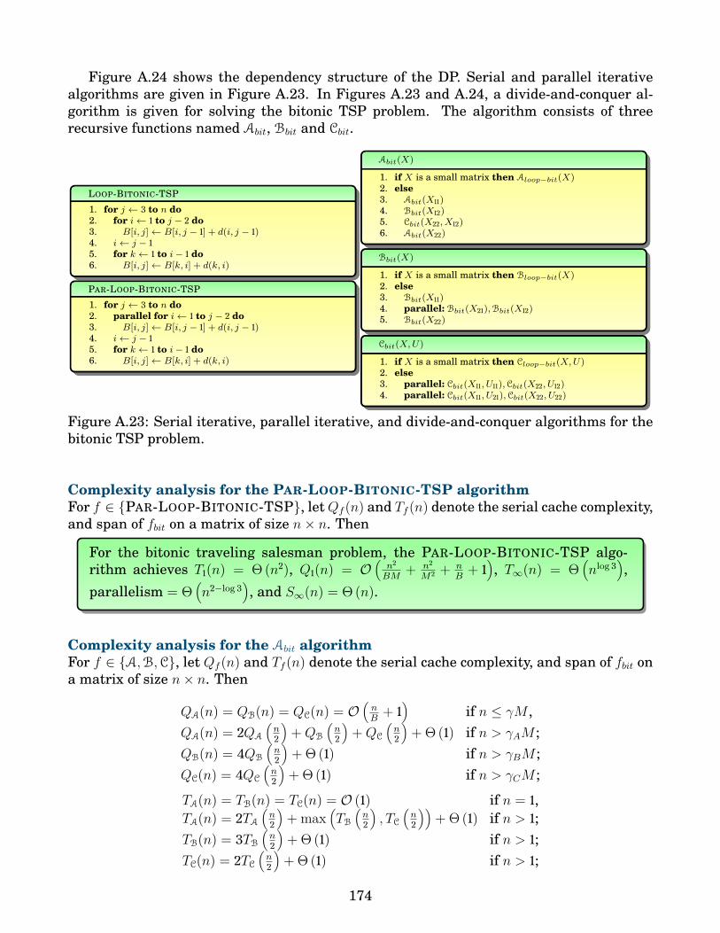
Figure A.24 shows the dependency structure of the DP. Serial and parallel iterativealgorithms are given in Figure A.23. In Figures A.23 and A.24, a divide-and-conquer al-gorithm is given for solving the bitonic TSP problem. The algorithm consists of threerecursive functions named Abit, Bbit and Cbit.

LOOP-BITONIC-TSP

1. for j ← 3 to n do2. for i← 1 to j − 2 do3. B[i, j]← B[i, j − 1] + d(i, j − 1)4. i← j − 15. for k ← 1 to i− 1 do6. B[i, j]← B[k, i] + d(k, i)

PAR-LOOP-BITONIC-TSP

1. for j ← 3 to n do2. parallel for i← 1 to j − 2 do3. B[i, j]← B[i, j − 1] + d(i, j − 1)4. i← j − 15. for k ← 1 to i− 1 do6. B[i, j]← B[k, i] + d(k, i)

Abit(X)

1. if X is a small matrix then Aloop−bit(X)2. else3. Abit(X11)4. Bbit(X12)5. Cbit(X22, X12)6. Abit(X22)

Bbit(X)

1. if X is a small matrix then Bloop−bit(X)2. else3. Bbit(X11)4. parallel: Bbit(X21),Bbit(X12)5. Bbit(X22)

Cbit(X,U)

1. if X is a small matrix then Cloop−bit(X,U)2. else3. parallel: Cbit(X11, U11),Cbit(X22, U12)4. parallel: Cbit(X11, U21),Cbit(X22, U22)

Figure A.23: Serial iterative, parallel iterative, and divide-and-conquer algorithms for thebitonic TSP problem.

Complexity analysis for the PAR-LOOP-BITONIC-TSP algorithmFor f ∈ PAR-LOOP-BITONIC-TSP, letQf (n) and Tf (n) denote the serial cache complexity,and span of fbit on a matrix of size n× n. Then

For the bitonic traveling salesman problem, the PAR-LOOP-BITONIC-TSP algo-rithm achieves T1(n) = Θ (n2), Q1(n) = O

(n2

BM+ n2

M2 + nB

+ 1), T∞(n) = Θ

(nlog 3

),

parallelism = Θ(n2−log 3

), and S∞(n) = Θ (n).

Complexity analysis for the Abit algorithmFor f ∈ A,B,C, let Qf (n) and Tf (n) denote the serial cache complexity, and span of fbit ona matrix of size n× n. Then


+ 1)

if n ≤ γM ,QA(n) = 2QA

(n2

)+QB

(n2

)+QC

(n2

)+ Θ (1) if n > γAM ;

QB(n) = 4QB

(n2

)+ Θ (1) if n > γBM ;

QC(n) = 4QC

(n2

)+ Θ (1) if n > γCM ;


(n2

)+ max

(TB(n2

), TC

(n2

))+ Θ (1) if n > 1;

TB(n) = 3TB(n2

)+ Θ (1) if n > 1;

TC(n) = 2TC(n2

)+ Θ (1) if n > 1;

174

Figure A.24: Top right: Dependency structure of the bitonic TSP DP. Rest: A divide-and-conquer algorithm for solving the problem.

where, γ, γA, γB, and γC are suitable constants. Solving, QA(n) = O(n2

BM+ n2

M2 + nB

+ 1)

andTA(n) = Θ

(nlog 3

).

For the bitonic traveling salesman problem, the Abit algorithm achieves T1(n) =Θ (n2), Q1(n) = O

(n2

BM+ n2

M2 + nB

+ 1), T∞(n) = Θ

(nlog 3

), parallelism = Θ

(n2−log 3

),

and S∞(n) = Θ (n).

A.10 Cocke-Younger-Kasami algorithmThe CYK algorithm [Hays, 1962,Younger, 1967,Kasami, 1965] was invented by John Cocke,Daniel Younger, and Tadao Kasami. It is a parsing algorithm used to parse context-free

175

grammars (given in Chomsky normal form (CNF)) and was used in compilers. It is one ofthe most efficient parsing algorithms.

We are given a string X = 〈x1, x2, . . . , xn〉 and a context-free grammar G = (V,∑, R, S),where V is a set of variables (or non-terminal symbols),

∑is a finite set of terminal symbols,

R = R1, R2, . . . , Rt : V → (V ∪∑)∗ is a finite set of rules, and S is a start variable chosenfrom V . We set P [i, j, c] to true provided substring Xij = xixi+1 . . . xi+j−1 can be generatedfrom rule Rc ∈ R, and to false otherwise. Then

P [i, j, c] =

true if j = 1 and Rc → xi,true if P [i, k, a] = P [i+ k, j − k, b] = true, k ∈ [1, i− 1] and Rc → RaRb,false otherwise.

(A.12)The dependency graph of the CYK algorithm is given in Figure A.25. A divide-and-

conquer algorithm (developed in collaboration with Jesmin Jahan Tithi) is given in FigureA.25. Note that the divide-and-conquer structure is exactly identical to that of the paren-thesis problem (Section A.2) and hence the complexity analysis similar as given in theparenthesis problem. In fact, through a different parameterization of the DP recurrence,we can end up with a DP recurrence that is very similar to that of the parenthesis problem.

For the CYK DP recurrence, the ACYK algorithm achieves T1(n) = Θ (n3), Q1(n) =O(

n3

B√M

+ n3

M+ n2

B+ n

), T∞(n) = Θ

(nlog 3

), parallelism = Θ

(n3−log 3

), and S∞(n) =

Θ (n2).

A.11 Binomial coefficientA binomial coefficient, denoted C(n, k) is the number of combinations (or subsets) of kelements taken fro a set of n elements. The term is called so because it comes from thecoefficients of the expansion of the binomial formula:

(a+ b)n = C(n, 0)an + · · ·+ C(n, k)an−kbk + · · ·+ C(n, n)bn.

Binomial coefficient can be computed with the recurrence

C(n, k) =

0 if k = 0 or k ≥ n,

C(n− 1, k − 1) + C(n− 1, k) if k ∈ [1, n− 1].

Figure A.26 shows the dependency graph for the problem. If we want to compute thebinomial coefficient C[n, k], then the part of the DP table that will be computed is shownin the figure. The first part consists of the region C[0 . . . k, 0 . . . k] in which the lower righttriangular region will be filled. The second part consists of the rectangular region C[k +1 . . . n, 0 . . . k].

Figure A.26 shows serial and parallel iterative algorithms to compute a binomial coeffi-cient. A divide-and-conquer algorithm is also given to solve the problem. It consists of tworecursive functions ABC and BBC . The function ABC fills a lower right-triangular regionand the function BBC fills a square region. This function can be easily extended / modified

176

Figure A.25: Top left: Dependency graph for the CYK algorithm Rest: A divide-and-conquer algorithm.

to work for generic rectangular matrices. For simplicity and pedagogical reasons we showthe working of the BBC function for square matrices only.

Complexity analysis for the PAR-LOOP-BINOMIAL-COEFFICIENT algorithmLet Qf (n, k) and Tf (n, k) denote the serial cache complexity, and span ofPAR-LOOP-BINOMIAL-COEFFICIENT with parameters n and k. ThenQf (n, k) = Θ

(n ·(kB

+ 1))

=Θ(nkB

+ n)

and Tf (n, k) = Θ (n · (log k + Θ (1))) = Θ (n log k).

For the binomial coefficient problem, the PAR-LOOP-BINOMIAL-COEFFICIENT al-gorithm achieves T1(n, k) = Θ (nk), Q1(n, k) = Θ

(nkB

+ n), T∞(n, k) = Θ (n log k), par-

allelism = Θ(

klog k

), and S∞(n) = Θ (k).

Complexity analysis for the D&C-BINOMIAL-COFFICIENT algorithmLet QA(k) and QB(n, k) denote the serial cache complexities and TA(k) and TB(n, k) denotethe span of the respective functions for parameters n and k. Then

177

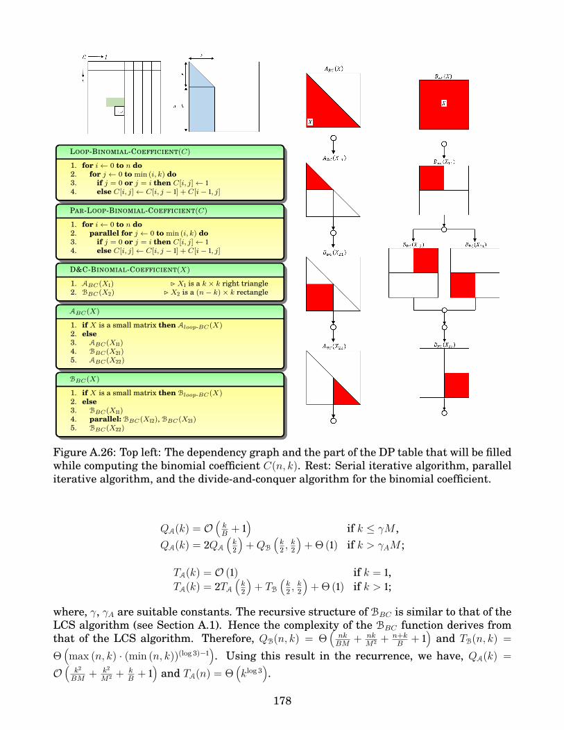
LOOP-BINOMIAL-COEFFICIENT(C)

1. for i← 0 to n do2. for j ← 0 to min (i, k) do3. if j = 0 or j = i then C[i, j]← 14. else C[i, j]← C[i, j − 1] + C[i− 1, j]

PAR-LOOP-BINOMIAL-COEFFICIENT(C)

1. for i← 0 to n do2. parallel for j ← 0 to min (i, k) do3. if j = 0 or j = i then C[i, j]← 14. else C[i, j]← C[i, j − 1] + C[i− 1, j]

D&C-BINOMIAL-COEFFICIENT(X)

1. ABC(X1) B X1 is a k × k right triangle2. BBC(X2) B X2 is a (n− k)× k rectangle

ABC(X)

1. if X is a small matrix then Aloop-BC(X)2. else3. ABC(X11)4. BBC(X21)5. ABC(X22)

BBC(X)

1. if X is a small matrix then Bloop-BC(X)2. else3. BBC(X11)4. parallel: BBC(X12), BBC(X21)5. BBC(X22)

Figure A.26: Top left: The dependency graph and the part of the DP table that will be filledwhile computing the binomial coefficient C(n, k). Rest: Serial iterative algorithm, paralleliterative algorithm, and the divide-and-conquer algorithm for the binomial coefficient.

QA(k) = O(kB

+ 1)

if k ≤ γM ,QA(k) = 2QA

(k2

)+QB

(k2 ,

k2

)+ Θ (1) if k > γAM ;

TA(k) = O (1) if k = 1,TA(k) = 2TA

(k2

)+ TB

(k2 ,

k2

)+ Θ (1) if k > 1;

where, γ, γA are suitable constants. The recursive structure of BBC is similar to that of theLCS algorithm (see Section A.1). Hence the complexity of the BBC function derives fromthat of the LCS algorithm. Therefore, QB(n, k) = Θ

(nkBM

+ nkM2 + n+k

B+ 1

)and TB(n, k) =

Θ(max (n, k) · (min (n, k))(log 3)−1

). Using this result in the recurrence, we have, QA(k) =

O(k2

BM+ k2

M2 + kB

+ 1)

and TA(n) = Θ(klog 3

).

178

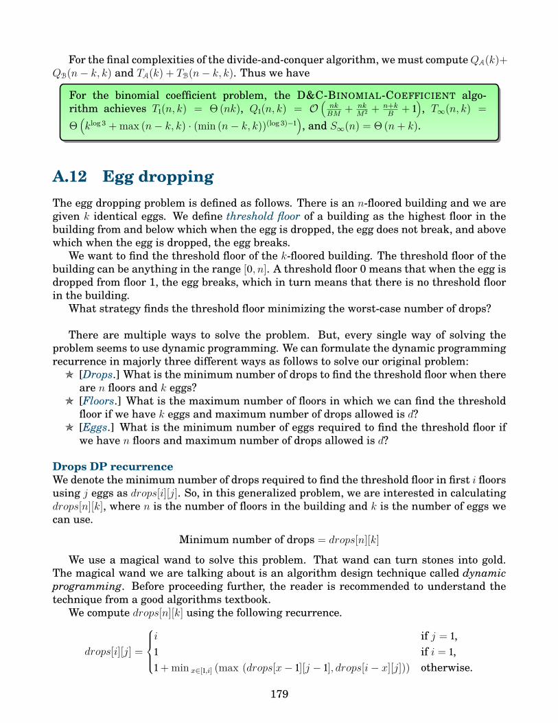
For the final complexities of the divide-and-conquer algorithm, we must computeQA(k)+QB(n− k, k) and TA(k) + TB(n− k, k). Thus we have

For the binomial coefficient problem, the D&C-BINOMIAL-COEFFICIENT algo-rithm achieves T1(n, k) = Θ (nk), Q1(n, k) = O

(nkBM

+ nkM2 + n+k

B+ 1

), T∞(n, k) =

Θ(klog 3 + max (n− k, k) · (min (n− k, k))(log 3)−1

), and S∞(n) = Θ (n+ k).

A.12 Egg droppingThe egg dropping problem is defined as follows. There is an n-floored building and we aregiven k identical eggs. We define threshold floor of a building as the highest floor in thebuilding from and below which when the egg is dropped, the egg does not break, and abovewhich when the egg is dropped, the egg breaks.

We want to find the threshold floor of the k-floored building. The threshold floor of thebuilding can be anything in the range [0, n]. A threshold floor 0 means that when the egg isdropped from floor 1, the egg breaks, which in turn means that there is no threshold floorin the building.

What strategy finds the threshold floor minimizing the worst-case number of drops?

There are multiple ways to solve the problem. But, every single way of solving theproblem seems to use dynamic programming. We can formulate the dynamic programmingrecurrence in majorly three different ways as follows to solve our original problem:

O [Drops.] What is the minimum number of drops to find the threshold floor when thereare n floors and k eggs?

O [Floors.] What is the maximum number of floors in which we can find the thresholdfloor if we have k eggs and maximum number of drops allowed is d?

O [Eggs.] What is the minimum number of eggs required to find the threshold floor ifwe have n floors and maximum number of drops allowed is d?

Drops DP recurrenceWe denote the minimum number of drops required to find the threshold floor in first i floorsusing j eggs as drops[i][j]. So, in this generalized problem, we are interested in calculatingdrops[n][k], where n is the number of floors in the building and k is the number of eggs wecan use.

Minimum number of drops = drops[n][k]

We use a magical wand to solve this problem. That wand can turn stones into gold.The magical wand we are talking about is an algorithm design technique called dynamicprogramming. Before proceeding further, the reader is recommended to understand thetechnique from a good algorithms textbook.

We compute drops[n][k] using the following recurrence.

drops[i][j] =

i if j = 1,1 if i = 1,1 + min x∈[1,i] (max (drops[x− 1][j − 1], drops[i− x][j])) otherwise.

179

The base cases when j = 1 (1 egg) and i = 1 (1 floor) is straightforward. The recursioncase for i floors and j eggs goes like this. If we drop an egg from floor x ∈ [1, i], there canbe two cases: (i) the egg breaks, in which case we are left with j − 1 eggs and we need totest floors in the range [1, i− 1]. Here, the total number of drops is 1+ drops[x− 1][j− 1]; and(ii) the egg does not break, in which case we are left with j eggs and we need to test floorsin the range [x+ 1, i]. Here, the total number of drops is 1 + drops[i− x][j]. We consider themaximum of the two cases (which represents the worst-case) and take the minimum of allmaximums by varying x in the range [1, i].

Figure A.28 gives the dependency structure of the drops[i][j] recurrence. Figure A.27gives a serial iterative DP algorithm to compute drops[n][k]. In Figure A.28, we presenta divide-and-conquer algorithm to solve the drops[i][j] DP recurrence. For simplicity ofexposition, we consider n = k. In [Frigo et al., 1999], a divide-and-conquer algorithmwas presented to solve the matrix multiplication problem for generic matrices. Using theideas presented in that paper, it is possible to extend our divide-and-conquer algorithm tocompute drops[n][k] for generic values of n and k.

The divide-and-conquer algorithm consists of three functions AED,BED, and CED. TheBED function is special. It reads from the region it writes to. Hence, several possibledependencies of cells are combined into that function. In the directed acyclic graph (DAG)of the BED function, only two parameters X and V are shown in the diagram. The functionBED(〈X, V,X〉, 〈X,X, V 〉, 〈X,X,X〉) is represented as BED(X, V ) for simplicity.

Improved algorithm. The iterative DP algorithm from Figure A.27 computes only theminimum number of drops required to find the threshold floor and not the informationabout the threshold floor and which egg has to be dropped from which floor. The algorithmcan be modified suitably to find this extra information as well. Though the algorithm is cor-rect and computes the optimum number of drops, it executes slow and its time complexityis Θ (n2k).

The algorithm’s runtime can be reduced to Θ (nk log n). We can find min x∈[1,i](max (drops[x−1][j−1], drops[i−x][j])) in Θ (log n) time using binary search. The reason is as follows. Whenx is a variable, drops[x− 1][j − 1] is an increasing function and drops[i− x][j] is a decreasingfunction and hence max (drops[x− 1][j − 1], drops[i− x][j]) will have a global minimum. Thisglobal minimum can be found using a variant of binary search.

We can further reduce the runtime to Θ (nk). We store the optimal x for every cell ofthe drops DP table. When we want to find the optimal x of a new cell, we make use of theoptimal x of its previous cells.

The plot of drops[n][k] for varying n is given in Figure A.29.

Complexity analysis for the AED algorithmFor f ∈ A,B,C, let Qf (n) and Tf (n) denote the serial cache complexity, and span of fEDon a matrix of size n× n. Then

QA(n) = QB(n) = QC(n) = O(n2

B+ 1

)if n2 ≤ γM ,

QA(n) = 2(QA

(n2

)+QB

(n2

)+QC

(n2

))+ Θ (1) if n2 > γAM ;

QB(n) = 4(QB

(n2

)+QC

(n2

))+ Θ (1) if n2 > γBM ;

QC(n) = 8QC

(n2

)+ Θ (1) if n2 > γCM ;

180

K-EGGS-PUZZLE(n, k) B Θ(n2k)

Input: Number of floors n and number of eggs kOutput: Minimum number of drops drops[n][k]1. for i← 1 to n do drops[i][1]← i2. for j ← 1 to k do3. drops[0][j]← 0; drops[1][j]← 14. for i← 2 to n do5. for j ← 2 to k do6. min← i7. for x← 1 to i do8. max← MAX(drops[x− 1][j − 1], drops[i− x][j])9. if max < min then min← max

10. drops[i][j]← min+ 111. return drops[n][k]

drops[i][j]

drops[i− x][j]

drops[x− 1][j − 1]

i

x

n

(egg does not break)

(egg breaks)

1

Figure A.27: Left: An algorithm to solve the k eggs problem for n floors. Right: The coreidea for the algorithm.

TA(n) = TB(n) = TC(n) = O (1) if n = 1,TA(n) = 2

(TA(n2

)+ TB

(n2

))+ TC

(n2

)+ Θ (1) if n > 1;

TB(n) = 3TB(n2

)+ 4TC

(n2

)+ Θ (1) if n > 1;

TC(n) = 2TC(n2

)+ Θ (1) if n > 1;

where, γ, γA, γB, and γC are suitable constants. Solving, QA(n) = O(

n3

B√M

+ n3

M+ n2

B+ n

)and TA(n) = Θ

(nlog 3

).

For the egg dropping problem, the AED algorithm achieves T1(n) = Θ (n3), Q1(n) =O(

n3

B√M

+ n3

M+ n2

B+ n

), T∞(n) = Θ

(nlog 3

), parallelism = Θ

(n3−log 3

), and S∞(n) =

Θ (n2).

A.13 Sorting algorithmsSorting is a computational process of rearranging a multiset of items in ascending or de-scending order [Knuth, 1998]. It is one of the most fundamental problems in computerscience. Sorting is used in real-life scenarios. Smartphone contacts are sorted based onnames; students’ (resp. employees’ and patients’) profiles are sorted based on student ID(resp. employee ID and patient ID); knock-out wrestling tournaments are like priorityqueues to sort wrestlers based on muscle strength; passengers waiting in a queue to boarda bus sort themselves based on time-of-arrival; flight (or bus or train) information is sortedbased on time-of-departure; people posing for a group photo often sort themselves based onheight; importance given to different jobs and people are sorted based on priorities; to-be-worn dresses are usually sorted based on least-recently-used; and, research papers to toptheory conferences are sorted based on incomprehensibility.

Sorting is used as an intermediate step to solve several computer science problems[Skiena, 1998, Knuth, 1998] such as: bringing all items with the same identification to-gether, matching items in two or more files, searching for a specific value, testing if all ele-ments are unique, deleting duplicates, finding the kth largest element (selection problem),

181

Figure A.28: Top center: Dependency graph for the egg dropping problem. Rest: A divide-and-conquer algorithm for solving the problem by computing drops[n][n].

finding the kth most frequently occurring element, finding set union/intersection, findingthe closest pair of points, finding a convex hull, and so on. Even if sorting was totally use-less, it is an exceptionally interesting problem that leads to several stunning algorithmsand mind-blowing analyses. We remember a quote often credited to Richard Feynman,“Science is like sex, sometimes something useful comes out, but that is not the reason whywe do it.” Due to the reasons mentioned above, sorting is a well studied problem and has alarge literature.

Several algorithms have been discovered to solve the sorting problem. More than sixdecades of research has yielded over a hundred algorithms to solve the sorting problem,

182

012345678

0 2 4 6 8 10 12 14 16 18 20 22 24 26 28 30

dro

ps[

n][

k]

n

drops[n][k]

k = 2 k = 3 k = 10

1

10

100

1000

10000

100000

1000000

0 2 4 6 8 10 12 14 16 18 20

flo

ors

[d][

k]

d

floors[d][k]

k = 2 k = 3 k = 10

Figure A.29: Left: Plot for drops[n][k] when n is varying from 1 to 30 and k is fixed at 2, 3,or 10. Right: Plot for floors[d][k] when d is varying from 1 to 20 and k is fixed at 2, 3, or 10.

many of which are either minor or major variations of tens of standard algorithms. Thesorting algorithms can be classified as in-place or not-in-place, stable or unstable, iterativeor recursive, serial or parallel [Akl, 2014,Cole, 1988], internal memory or external memory,deterministic or randomized, adaptive [Estivill-Castro and Wood, 1992] or non-adaptive,and self-improving [Ailon et al., 2011] or non-self-improving.

In this section, we present recursive divide-and-conquer variants of bubble, selection,and insertion sorting algorithms.

Why care for divide-and-conquer algorithms?. Divide-and-conquer is an algorithmdesign strategy used to solve problems by breaking them into one or more subproblems,solving them, and combining their solutions to solve the original problem. Often, the sub-problems are independent and the divide-and-conquer algorithms are implemented recur-sively.

Divide-and-conquer algorithms have the following advantages:O They can be represented succinctly and can be analyzed for its complexities using

recurrence relations [Bentley, 1980].O They are usually efficient [Levitin, 2011] in the sense that they reduce the total num-

ber of computations.O They can be parallelized easily [Mou and Hudak, 1988].O They often are (or can be made) cache-efficient and cache-oblivious [Frigo et al., 1999,

Chatterjee et al., 2002,Frens and Wise, 1997].For example, some of the fastest sorting algorithms such as merge sort and quicksort

are based on recursive divide-and-conquer.3.

Why care for bubble, selection, & insertion sorts?. Among all sorting algorithms,bubble, selection, and insertion sorts [Levitin, 2011] are three of the most elementary al-gorithms that are widely taught to computer science students. The algorithms are popularmajorly because they are arguably simple, easy-to-remember, and easy-to-program.

From unreliable sources, it is known that there is a tribe in the Amazon forests calledZozo. Every night, a volunteer from the tribe makes sure that the people are sorted basedon age and they get their food share in that order. Interestingly, the tribe uses bubble sortto sort the people.

3The fastest sorting algorithm runs in O (1) time – simply call a sort() function from a standard library.:)

183

We too use bubble, selection, and insertion sorts depending on our moods and occasions.For stress management, we often recommend students to mentally sort the numbers from100 to 1 using insertion sort, unlike counting numbers from 100 to 1.

Model. Analogous to cache-oblivious model (or ideal-cache model) [Frigo et al., 1999], wedevelop a memory-oblivious model. In this model, a human mind is assumed to consistof a constant number of processing elements (or processors) and a hierarchy of memories(short-term and long-term), as shown in Figure A.30. The amount of information that canbe stored at memory levels near the processors are lesser than that those away from theprocessors. Similarly, time to access information from memory levels near the processorsis smaller than that of higher memory levels. Also, the number of memory levels, memorysizes, etc varies from person to person. It is important to note that the traditional cache-aware or external-memory (or analogously memory-aware) model is not suitable becausepeople do not know their memory sizes or the number of levels of memory they have.

When a processing element looks for some information in a memory-level and that in-formation is not found, that leads to a memory miss. The total number of memory misses ismeasured as memory-complexity. The better the memory complexity for an algorithm, thefewer the number of thoughts required to check different memory levels for informationand faster it is for the mind to execute the algorithm.

Divide-and-conquer variants of bubble, selection, & insertion sorts. Humans (i.e.,minds) heavily use bubble, selection, and insertion sorts because these algorithms are sim-ple and intuitive. On the other hand, computers (i.e., machines) heavily use merge sort andquicksort because these algorithms are very fast. Our aim is to improve the performanceof the elementary sorting algorithms and save billions of minutes of time for millions ofpeople in their sorting business.

In this section, we present divide-and-conquer variants of the elementary sorting al-gorithms. By the virtue of divide-and-conquer, such algorithms are memory-efficient andmemory-oblivious.

Shortest-term memory

……………

……………… …

………

………

………

Short-term memory

Longest-term memory

Processors

Figure A.30: Left: Place-holder of the human mind. Right: The memory-hierarchy of the humanmind.

Our divide-and-conquer algorithms are memory-oblivious. Any person can use it irre-spective of her/his memory hierarchy. The algorithms are provably memory-efficient too.This implies, the number of thoughts that accesses different memory levels to execute analgorithm in mind is minimized asymptotically and hence sorting can be done asymptoti-cally much faster.

Students complain about non-remembrance and older adults complain about forget-fulness. Clinical observation [Kral, 1962] shows that memory loss occurs significantly inaging individuals. In algorithmic terms, it can be called the memory-shrinkage problem.

184

Using the results from [Bender et al., 2014], we can prove that our divide-and-conquervariants of sorting algorithms are memory-adaptive in the sense that they work optimallyeven if the memory size changes dynamically. This implies, the young and the old can usethe proposed algorithms and minimize the time they take to sort out things.

In this section, we present divide-and-conquer variants of bubble, selection, and inser-tion sorts. Both recursive bubble and selection sorts use partition algorithms. On the otherhand, the recursive insertion sort uses a merge algorithm. We explain the logic of recursivebubble sort in more details. The explanation to other two algorithms can be extended in asimilar way.

Notations & terminologies. For all algorithms, we sort the n-sized array A[0..n − 1].For simplicity, we assume that n is a power of 2. In all recursive function calls, we usenotations such as `, h,m, ``, `h, r`, rh, etc, all of which represent the indices in the array A.The notations `,m, h mean low, mid, and high, respectively. Terms `` and rm mean lowin the left array and mid in the right array, respectively. Other terms can be defined in asimilar way. When a subproblem size h − ` + 1 or `h − `` + 1 becomes less than or equal tothe base case size b, then we execute an iterative base case kernel having an algorithm-dependent logic. The terms used in the section are summarized in Table A.1.

Symbol MeaningA array to be sortedn Input parameter

`, h,m Low, high, and mid`` Left subarray’s low indexrh Right subarray’s high index

I-BS Iterative bubble sortR-BS Recursive bubble sortP-BS Partition in bubble sortM-IS Merge in insertion sort

Table A.1: Standard notations used for the sorting algorithms. Other notations are such as I-SS,R-SS, etc are similarly defined.

Related work. Bubble sort [Friend, 1956, Gotlieb, 1963] is also called sinking sort, ex-change selection, shuttle sort, propagation, or push-down sort. Variations of bubble sortexists such as cocktail sort [Knuth, 1998] (a.k.a shaker sort, bidirectional bubble sort,shaker sort, ripple sort, or shuffle sort), where the direction of bubbling alternates be-tween left-to-right and right-to-left, and odd-even sort [Habermann, 1972] (a.k.a odd-eventransposition sort or brick sort).

Selection sort has several variants such as cocktail sort (a.k.a shaker sort or dual selec-tion sort), where both the minimum and maximum elements are found in every pass, andbingo sort [Bin, ], which scans the remaining elements to find the greatest value and shiftsall elements with that value to their final locations.

Insertion sort variants include Shell sort [Shell, 1959], where elements separated by adistance are compared; binary insertion sort, which uses binary search to find the exactlocation of the new elements to be inserted; binary merge sort, which uses binary inser-tion sort and merge sort; heap sort, where insertions and searches are performed with asophisticated data structure called a heap; and library sort [Bender et al., 2006b] (a.k.a

185

gapped insertion sort), where small number of spaces are left unused to make gaps for theelements to be inserted. Insertion sort is generally faster than selection sort which almostalways is faster than bubble sort.

The cache performance effects on sorting algorithms have been studied by [LaMarcaand Ladner, 1999]. The lower-bounds on sorting in external-memory model is given byAggarwal and Vitter [Aggarwal et al., 1988]. The serial cache-oblivious model was proposedin [Frigo et al., 1999].

I-BS(A,n)

1. for i← 0 to n− 1 do2. for j ← 0 to n− i− 1 do3. if A[j] > A[j + 1] then4. SWAP(A[j], A[j + 1])

I-SS(A,n)

1. for i← 0 to n− 1 do2. min← i3. for j ← i to n− 1 do4. if A[j] < A[min] then5. min← j6. SWAP(A[i], A[min])

I-IS(A,n)

1. for i← 1 to n− 1 do2. key ← a[i]3. for j ← i− 1 to 0 do4. if A[j] > key then5. A[j + 1]← A[j]6. A[j + 1]← key

Figure A.31: Standard iterative algorithms for bubble sort (I-BS), selection sort (I-SS), and in-sertion sort (I-IS). Optimizations are not shown for pedagogical reasons.

A.13.1 Bubble sort

Bubble sort is one of the simplest sorting algorithms that is taught in an undergraduatealgorithms course. Though it is a very slow algorithm takingO (n2) time to sort n elements,it is simple to understand and easy to program.

A simple iterative algorithm called I-BS is given in Figure A.31. It has n iterations. Ineach iteration i (∈ [0, n− 1)), every two adjacent elements j and j+ 1, where j ∈ [0, n− i− 1],are compared and sorted if they are not already in their sorted order. The number ofcomparisons at iteration i is n− i and at the end of the iteration, the array (i+ 1)th largestelement will be in its correct position.

A recursive divide-and-conquer variant of bubble sort called R-BS is shown in FigureA.32. The aim is to sort the entire array A[0..n− 1]. The function R-BS(A, `, h, n) sorts thesubarray A[`..h]. The initial invocation to the algorithm is by calling R-BS(A, 0, n − 1, n).The function R-BS in turn calls the P-BS function. The P-BS function is the partitionfunction for bubble sort that brings the smallest n/2 elements to the left half and thelargest n/2 elements to the right half of array A. Once the array A is partitioned, then theR-BS is recursively called onto the left and right halves in parallel to sort the two halves.After the two halves are sorted recursively, the entire array A[0..n− 1] will be sorted. Whenthe subproblem reaches the base case, it is sorted using the standard iterative bubble sortlogic.

The partition function P-BS(A, ``, `h, r`, rh, n) partitions the elements such that afterthe partition, the largest element in A[``..`h] will be less than or equal to the smallestelement in A[r`..rh]. The function works as follows.

In the base case, we use two loops: the outer-loop ranging over the right subarray andthe inner-loop ranging over the left subarray. Using a logic similar to that of iterativebubble sort, the largest elements in the left subarray are pushed to the right subarrayafter every iteration.

186

R-BS(A, `, h, n)

1. if (h− `+ 1) ≤ b then2. for i← ` to h do3. for j ← ` to `+ h− i− 1 do4. if A[j] > A[j + 1] then5. SWAP(A[j], A[j + 1])6. else7. m← (`+ h)/28. P-BS(A, `,m,m+ 1, h, n)9. parallel: R-BS(A, `,m, n),

R-BS(A,m+ 1, h, n)

P-BS(A, ``, `h, r`, rh, n)

1. if (`h− ``+ 1) ≤ b then2. for i← r` to rh do3. for j ← `` to `h− 1 do4. if A[j] > A[j + 1] then5. SWAP(A[j], A[j + 1])6. if A[`h] > A[i] then SWAP(A[`h], A[i])7. else8. `m← (``+ `h)/2; rm← (r`+ rh)/29. parallel: P-BS(A, ``, `m, r`, rm, n),

P-BS(A, `m+ 1, `h, rm+ 1, rh, n)10. parallel: P-BS(A, ``, `m, rm+ 1, rh, n),

P-BS(A, `m+ 1, `h, r`, rm, n)

Figure A.32: A recursive divide-and-conquer variant of bubble sort. Initial call to the recursivealgorithm is R-BS(A, 0, n− 1, n), where A[0..n− 1] is the array to be sorted.

In the recursion case, the P-BS calls itself four times. The reason for requiring fourfunction calls is simple. Let `m and rm be the midpoints of the left and right subarray,respectively. The left subarray A[``..`h] can be divided into two subarrays A[``..`m] andA[(`m + 1)..`h] and the right subarray A[r`..rh] can be divided into two subarrays A[r`..rm]and A[(rm + 1)..rh]. This means there are a total of four possible combinations of leftand right subsubarrays. The P-BS function invokes two functions that work on differentregions of the array, in parallel. In the next step, two more functions are invoked in parallelthat work on disjoint regions. After the four invocations the larger elements would havemoved to the right subarray leaving the smaller elements in the left subarray.

Theorem 14 (Bubble sort correctness). The divide-and-conquer variant of bub-ble sort algorithm i.e., R-BS correctly sorts the input array.

Proof. We use mathematical induction to prove the theorem. First we prove the correctnessof P-BS function. Then we prove R-BS correct. For simplicity, we assume that n and bare powers of 2 such that n ≥ b. We term A[``..``h] and A[r`..rh] as left and right inputsubarrays, respectively.(1) [Correctness of P-BS.]Basis. The logic of the base case when the input subarray is of size b is straightforward.The external loop runs b times and in each iteration, one of the larger elements sifts to theright subarray.Induction. We assume that P-BS works correctly when the input subarrays are of size 2kfor some k, such that 2k ≥ b. We need to prove that P-BS works for input subarrays of size2k+1.

LetQ1, Q2, Q3, andQ4, whereQ stands for “quarter”, represent the locationsA[``..`m], A[(`m+1)..`h], A[r`..rm], and A[(rm + 1)..rh], respectively, where each subarray is of size 2k. LetW,X, Y , and Z be the initial sets of numbers present at Q1, Q2, Q3, and Q4, respectively.Let SMALL(S1, S2) (resp. LARGE(S1, S2)) of two sets S1 and S2 of numbers represent a setconsisting of the smallest half (resp. largest half) of the numbers from sets S1 and S2. Also,let S1 ≤ S2 denote that all elements of S1 is less than or equal to all elements of S2.

After execution of line 8, the states of the four quarters of the array A are Q1 = W , Q2 =X, Q3 = Y , and Q4 = Z. After execution of line 9, the states of the four quarters of the array

187

A are: Q1 = SMALL(W,Y ), Q2 = SMALL(X,Z), Q3 = LARGE(W,Y ), and Q4 = LARGE(X,Z).After execution of line 10, the states of the four quarters of the array A are:

O Q1 = SMALL(SMALL(W,Y ),LARGE(X,Z))O Q2 = SMALL(SMALL(X,Z),LARGE(W,Y ))O Q3 = LARGE(SMALL(X,Z),LARGE(W,Y ))O Q4 = LARGE(SMALL(W,Y ),LARGE(X,Z))It is easy to see that

O Q1 ≤ Q4O Q2 ≤ Q3O Q1 ≤ SMALL(W,Y ) ≤ LARGE(W,Y ) ≤ Q3O Q2 ≤ SMALL(X,Z) ≤ LARGE(X,Z) ≤ Q4

As Q1 ≤ Q3, Q1 ≤ Q4, Q2 ≤ Q3, and Q2 ≤ Q4, the input subarrays of size 2k+1 have beenpartitioned.(2) [Correctness of R-BS.]Basis. The base case when the input subarray is of size b is exactly same as the standarditerative bubble sort and hence is correct.Induction. We assume that R-BS works correctly when the input subarrays are of size2k for some k, such that 2k ≥ b. We need to prove that R-BS works for input subarraysof size 2k+1. We know that the P-BS function is correct and hence after line 8, the leftsubarray (A[`..m]) and the right subarray (A[(m+ 1)..h]) would be partitioned such that thelargest element in the left subarray will not be greater than the smallest element in theright subarray. Then after line 9, we recursively sort the subarrays without affecting thepartition constraint and hence the total subarray will be sorted.

Complexity analysisFor function f ∈ I-BS,R-BS,P-BS, let Qf (n) and Tf (n) denote the serial cache complex-ity and span of f , respectively, to sort an n-sized array. Then

QI-BS(n) = ∑n−1i=0 Θ (((n− i)/B) + 1) = Θ (n2/B + n) .

QR-BS(n) = QP-BS(n) = O (n/B + 1) if n ≤ γM ,QR-BS(n) = 2QR-BS (n/2) +QP-BS (n/2) +O (1) if n > γM ,QP-BS(n) = 4QP-BS (n/2) +O (1) if n > γM .

TR-BS(n) = TP-BS(n) = O (1) if n = 1,TR-BS(n) = TR-BS (n/2) + TP-BS (n/2) +O (1) if n > 1,TP-BS(n) = 2TP-BS (n/2) +O (1) if n > 1.

where, γ is a suitable constant. The cache complexity of a subproblem of size n when it fitscache i.e., n ≤ γM , is Θ (n/B + 1) = O (M/B + 1). The cache complexity of a subproblemwhen it does not fit into cache is recursively computed using its subproblems. Solving therecurrences we get QR-BS(n) = O (n2/(BM) + n2/M 2 + n/B + n/M + 1) and TR-BS(n) = Θ (n).

The R-BS algorithm achieves T1(n) = Θ (n2), Q1(n) = O(n2

BM+ n2

M2 + nB

+ 1), T∞(n) =

Θ (n), parallelism = Θ (n), and S∞(n) = Θ (n).

188

A.13.2 Selection sortSelection sort is another slow running sorting algorithm that sorts n numbers in O (n2)time.

An iterative algorithm called I-SS is given in Figure A.31. The algorithm has n itera-tions. In each iteration i ∈ [0, n− 1], the position of the minimum element, denoted by minis found in the range A[i..n − 1]. Then the elements A[min] and A[i] are swapped, whichmakes sure that after iteration i, the ith smallest element is in its correct position.

R-SS(A, `, h, n)

1. if (h− `+ 1) ≤ b then2. for i← ` to h− 1 do3. min← i4. for j ← i+ 1 to h do5. if A[j] < A[min] then6. min← j7. if min , i then8. SWAP(A[i], A[min])9. else

10. m← (`+ h)/211. P-SS(A, `,m,m+ 1, h, n)12. parallel: R-SS(A, `,m, n),

R-SS(A,m+ 1, h, n)

P-SS(A, ``, `h, r`, rh, n)

1. if (`h− ``+ 1) ≤ b then2. for i← `` to `h do3. min← i4. for j ← r` to rh do5. if A[j] < A[min] then min← j6. if min , i then7. SWAP(A[i], A[min])8. else9. `m← (``+ `h)/2; rm← (r`+ rh)/2

10. parallel: P-SS(A, ``, `m, r`, rm, n),P-BS(A, `m+ 1, `h, rm+ 1, rh, n)

11. parallel: P-SS(A, ``, `m, rm+ 1, rh, n),P-SS(A, `m+ 1, `h, r`, rm, n)

Figure A.33: A recursive divide-and-conquer variant of selection sort. Initial call to the recursivealgorithm is R-SS(A, 0, n− 1, n), where A[0..n− 1] is the array to be sorted.

A recursive divide-and-conquer variant of selection sort R-SS is shown in Figure A.33.The initial invocation to the algorithm is by calling R-SS(A, 0, n − 1, n). The recursivestructure of the algorithm is exactly the same as that of bubble sort. The R-SS functioninvokes P-SS function to partition the array A into two halves where the largest elementin the first half is lesser than or equal to the smallest element in the second half. Afterthe partition, the R-SS functions are invoked on the two halves to sort them recursively.The partition function P-SS calls itself four times: two P-SS functions in two parallelsteps. The only difference between the bubble sort and selection sort divide-and-conqueralgorithms are the base cases of R-SS and P-SS functions.

The base case kernel of R-SS function is equivalent to that of the standard iterativeI-SS algorithm. The P-SS(A, ``, `h, r`, rh, n) function base case kernel in each iterationfinds an element that belongs to the left subarray and pushes it into the left subarray.After several iterations, the elements in the two subarrays would be partitioned in such away that the largest element in the left subarray A[``..`h] would be lesser than or equal tothe smallest element in the right subarray A[r`..rh].

Theorem 15 (Selection sort correctness). The divide-and-conquer variant of se-lection sort algorithm i.e., R-SS correctly sorts the input array.

Proof. We use mathematical induction to prove the theorem. First we prove the correctnessof P-SS function. Then we prove R-SS correct. For simplicity, we assume that n and bare powers of 2 such that n ≥ b. We term A[``..``h] and A[r`..rh] as left and right inputsubarrays, respectively.(1) [Correctness of P-SS.]Basis. The logic of the base case when the input subarray is of size b is straightforward.

189

The external loop runs b times. In each iteration, we find the index of one the smallestelements in the right subarray and if the element on the right subarray is less than anelement in the left subarray, then we swap it. In this way, the smallest b elements will siftto the left subarray.Induction. The argument is similar to that given in Theorem 14.(2) [Correctness of R-SS.]Basis. The base case when the input subarray is of size b is exactly same as the standarditerative selection sort and hence is correct.Induction. The argument is similar to that given in Theorem 14.

Complexity analysisFor function f ∈ I-SS,R-SS,P-SS, letQf (n) and Tf (n) denote the serial cache complexityand span of f , respectively, to sort an n-sized array. Then

QI-SS(n) = ∑n−1i=0 Θ (((n− i)/B) + 1) = Θ (n2/B + n) .

QR-SS(n) = QP-SS(n) = O (n/B + 1) if n ≤ γM ,QR-SS(n) = 2QR-SS (n/2) +QP-SS (n/2) +O (1) if n > γM ,QP-SS(n) = 4QP-SS (n/2) +O (1) if n > γM .TR-SS(n) = TP-SS(n) = O (1) if n = 1,TR-SS(n) = TR-SS (n/2) + TP-SS (n/2) +O (1) if n > 1,TP-SS(n) = 2TP-SS (n/2) +O (1) if n > 1.

where, γ is a suitable constant. Solving the recurrences we get TR-SS(n) = Θ (n) andQR-SS(n) = O (n2/(BM) + n2/M 2 + n/B + n/M + 1).

The R-SS algorithm achieves T1(n) = Θ (n2), Q1(n) = O(n2

BM+ n2

M2 + nB

+ 1), T∞(n) =

Θ (n), parallelism = Θ (n), and S∞(n) = Θ (n).

A.13.3 Insertion sortInsertion sort is a pretty fast algorithm that sorts a set of n elements in O (n2) worst casetime and O (n log n) average case time.

An iterative insertion sort algorithm is given in Figure A.31. The algorithm has n − 1iterations. In iteration i (∈ [1, n − 1), the array element A[i] will be inserted in a sortedposition in the range A[0 . . . i − 1]. After each iteration i, the subarray A[0 . . . i] will besorted. The runtime complexity is data-sensitive.

A recursive divide-and-conquer variant of the insertion sort is given in Figure A.34. Theinitial invocation to the algorithm is by calling R-IS(A, 0, n− 1, n). The recursive structureof the algorithm is similar to bubble and selection sorts but order of function calls aredifferent. The R-IS function calls itself twice to sort the left and right halves separatelyand simultaneously. Then it invokes M-IS function to merge the elements from the twohalves using the logic of the iterative insertion sort. After the merge, the entire arraywould have been sorted.

The merge function M-IS calls itself a total of three times: the first two calls in paralleland then a third serial call. The first call M-IS(A, ``, `m, r`, rm, n) brings the smallest ele-ments to A[``..`m] in sorted order. The second call M-IS(A, `m+1, `h, rm+1, rh, n) brings the

190

R-IS(A, `, h, n)

1. if (h− `+ 1) ≤ b then2. for i← `+ 1 to h do3. key ← A[i]4. j ← i− 15. while j ≥ ` & A[j] > key do6. A[j + 1]← A[j]7. j ← j − 18. A[j + 1]← key9. else

10. m← (`+ h)/211. parallel: R-IS(A, `,m, n),

R-IS(A,m+ 1, h, n)12. M-IS(A, `,m,m+ 1, h, n)

M-IS(A, ``, `h, r`, rh, n)

1. if (`h− ``+ 1) ≤ b then2. if A[`h] > A[r`] then3. for i← r` to rh do4. key ← A[i]; j ← i− 15. while j ≥ r` & A[j] > key do6. A[j + 1]← A[j]; j ← j − 17. if A[`h] > key then8. A[r`]← A[`h]; j ← lh− 19. while j ≥ `` & A[j] > key do

10. A[j + 1]← A[j]; j ← j − 111. A[j + 1]← key12. else13. `m← (``+ `h)/2; rm← (r`+ rh)/214. parallel: M-IS(A, ``, `m, r`, rm, n),

M-IS(A, `m+ 1, `h, rm+ 1, rh, n)15. M-IS(A, `m+ 1, `h, r`, rm, n)

Figure A.34: A recursive divide-and-conquer variant of insertion sort. Initial call to the recursivealgorithm is R-IS(A, 0, n− 1, n), where A[0..n− 1] is the array to be sorted.

largest elements to A[rm+ 1..rh] in sorted order. The third call M-IS(A, `m+ 1, `h, r`, rm, n)brings the remaining elements to A[`m+ 1..rm] in the sorted order.

The base case kernel of R-IS function is equivalent to that of the I-IS algorithm. TheM-IS(A, ``, `h, r`, rh, n) function base case kernel merges two sorted subarrays into sortedorder (retaining the sorted elements in those two input subarrays). In iteration k, thekth element of the right subarray gets merged with its previous elements (in the rightsubarray) and with the elements of left subarray. After rh− r`+ 1 iterations, the elementsin the two subarrays would be merged into a sorted order – the left subarray will be sorted,the right subarray will be sorted, and the last element of the left subarray will be less thanor equal to the first element of the right subarray.

Theorem 16 (Insertion sort correctness). The divide-and-conquer variant of in-sertion sort algorithm i.e., R-IS correctly sorts the input array.

Proof. We use mathematical induction to prove the theorem. First we prove the correctnessof M-IS function. Then we prove R-IS correct. For simplicity, we assume that n and b arepowers of 2 such that n ≥ b. We termA[``..`h] andA[r`..rh] as left and right input subarrays,respectively.(1) [Correctness of M-IS.]Basis. The logic of the base case when the input subarray is of size b is straightforward.The external loop runs b times for all elements in the right subarray. In each iteration,the element from the right subarray is inserted into its correct position towards it left byshifting elements.Induction. We assume that M-IS works correctly when the input subarrays are of size 2kfor some k, such that 2k ≥ b. We need to prove that M-IS works for input subarrays of size2k+1.

LetQ1, Q2, Q3, andQ4, whereQ stands for “quarter”, represent the locationsA[``..`m], A[(`m+1)..`h], A[r`..rm], and A[(rm + 1)..rh], respectively, where each subarray is of size 2k. LetW,X, Y , and Z be the initial sets of numbers present at Q1, Q2, Q3, and Q4, respectively.Let SMALL(S1, S2) (resp. LARGE(S1, S2)) of two sets S1 and S2 of numbers represent a setconsisting of the smallest half (resp. largest half) of the numbers from sets S1 and S2. Also,

191

let S1 ≤ S2 denote that all elements of S1 is less than or equal to all elements of S2. As theinput subarrays are sorted we have W ≤ X and hence we can write W = SMALL(W,X)and X = LARGE(W,X). Similarly, Y ≤ Z and therefore we can write Y = SMALL(Y, Z) andZ = LARGE(Y, Z).

After execution of line 13, the states of the four quarters of the array A are Q1 = W ,Q2 = X, Q3 = Y , and Q4 = Z. After execution of line 14, the states of the four quartersof the array A are: Q1 = SMALL(W,Y ), Q2 = SMALL(X,Z), Q3 = LARGE(W,Y ), and Q4 =LARGE(X,Z). After execution of line 15, the states of the four quarters of the array A are:

O Q1 = SMALL(W,Y )O Q2 = SMALL(SMALL(X,Z),LARGE(W,Y ))O Q3 = LARGE(SMALL(X,Z),LARGE(W,Y ))O Q4 = LARGE(X,Z)It is easy to see that

O Q1 = SMALL(SMALL(W,X), SMALL(Y, Z)) = SMALL(SMALL(W,Y ), SMALL(X,Z)) ≤Q2

O Q2 ≤ Q3O Q3 ≤ LARGE(LARGE(X,Z),LARGE(W,Y )) = LARGE(LARGE(W,X),LARGE(Y, Z)) =

Q4

As Q1 ≤ Q2 ≤ Q3 ≤ Q4, the input subarrays of size 2k+1 have been merged.(2) [Correctness of R-IS.]Basis. The base case when the input subarray is of size b is exactly same as the standarditerative insertion sort and hence is correct.Induction. We assume that R-IS works correctly when the input subarrays are of size 2kfor some k, such that 2k ≥ b. We need to prove that R-IS works for input subarrays of size2k+1. We know that the R-IS function is correct and hence after line 11, the left subarray(A[`..m]) would be sorted and the right subarray (A[(m+ 1)..h]) would be sorted. Then afterline 12, we merge the two subarrays. As we have shown that the merge function M-IS iscorrect, the entire subarray of size 2k+1 would be merged and sorted.

Complexity analysisFor function f ∈ I-IS,R-IS,M-IS, let Wf (n), Qf (n), and Tf (n) denote the work, serialcache complexity, and span of f , respectively, to sort an n-sized array. We use the term Winstead of T1 for simplicity. Then

QI-IS(n) = ∑n−1i=0 O (((n− i)/B) + 1) = O (n2/B + n) .

WR-IS(n) = WM-IS(n) = O (1) if n = 1,WR-IS(n) = 2WR-IS (n/2) +WM-IS (n/2) + Θ (1) if n > 1,WM-IS(n) = 3WM-IS (n/2) + Θ (1) if n > 1.

QR-IS(n) = QM-IS(n) = O (n/B + 1) if n ≤ γM ,QR-IS(n) = 2QR-IS (n/2) +QM-IS (n/2) +O (1) if n > γM ,QM-IS(n) = 3QM-IS (n/2) +O (1) if n > γM .

TR-IS(n) = TM-IS(n) = O (1) if n = 1,TR-IS(n) = TR-IS (n/2) + TM-IS (n/2) +O (1) if n > 1,TM-IS(n) = 2TM-IS (n/2) +O (1) if n > 1.

192

where, γ is a suitable constant. Solving the recurrences we get WR-IS(n) = O(nlog 3

),

TR-IS(n) = O (n), and QR-IS(n) = O(nlog 3/(BM (log 3)−1) + nlog 3/M log 3 + n/B + n/M + 1

). All

logarithms are taken to the base 2.We compute the serial cache complexity of R-IS. We initially find QM-IS and then use it

to compute QR-IS. We assume that n/2k = γM for some γ.

QM-IS (n) ≤ 3QM-IS

(n

2

)+ c = 3

(3QM-IS

(n

22)

+ c)

+ c = 32QM-IS

(n

22)

+ 3c+ c

= 3kQM-IS

(n

2k)

+ c(3k−1 + 3k−2 + · · ·+ 1

)≤ 3k

(QM-IS

(n

2k)

+ c)≤ c

(n

M

)log 3 (MB

+ 1)

= O(

nlog 3

BM log 3−1 + nlog 3

M log 3

)

Plugging in QM-IS value into the recurrence of QR-IS, we get

QR-IS (n) ≤ 2QR-IS

(n

2

)+QM-IS

(n

2

)+ c ≤ 2QR-IS

(n

2

)+ c

nlog 3

BM log 3−1 + cnlog 3

M log 3 + c

≤ 2

2QR-IS

(n

22)

+ c

(n2

)log 3

BM log 3−1 + c

(n2

)log 3

M log 3 + c

+ cnlog 3


M log 3 + c

= 22QR-IS

(n

22)

+ 2c+ c+ 2c

(n2

)log 3

BM log 3−1 + 2c

(n2

)log 3

M log 3 + cnlog 3


M log 3

= 22QR-IS

(n

22)

+ c

(nlog 3


M log 3

)(1 + 1

2log 3−1

)+ c (2 + 1)

≤ 2kQR-IS

(n

2k)

+ c

(nlog 3


M log 3

)(1 + · · ·+ 1

(2log 3−1)k−1

)+ c

(2k−1 + · · ·+ 1

)≤ c

n

M

(M

B+ 1

)+ c

nlog 3


M log 3

= O(

nlog 3


M log 3 + n

B+ n

M+ 1

)

The R-IS algorithm achieves T1(n) = O(nlog 3

), Q1(n) =

O(

nlog 3

BM(log 3)−1 + nlog 3

M log 3 + nB

+ nM

+ 1), T∞(n) = O (n), parallelism = Θ

(n(log 3)−1

),

and S∞(n) = Θ (n).

A.13.4 Experimental resultsTable A.2 summarizes the theoretical complexities of our algorithms. This section presentsempirical results showing the performance improvements from high parallelism, bettercache complexity, and less work.

193

Iterative algorithm Divide-and-conquer algorithmProblem T1 Q1 T∞ T1/T∞ T1 Q1 T∞ T1/T∞

Bubble sort [Levitin, 2011] Θ (n2) Θ(n2

B

)Θ (n2) Θ (1) Θ (n2) O

(n2

BM

)Θ (n) Θ (n)

Selection sort [Levitin, 2011] Θ (n2) Θ(n2

B

)Θ (n2) Θ (1) Θ (n2) O

(n2

BM

)Θ (n) Θ (n)

Insertion sort [Levitin, 2011] O (n2) O(n2

B

)O (n2) Θ (1) O

(nlog 3

)O(

nlog 3

BM log 3−1

)O (n) Ω (n)

Table A.2: Work (T1), serial cache complexity (Q1), span (T∞), and parallelism (T1/T∞) ofiterative and recursive divide-and-conquer algorithms for the bubble, selection, and inser-tion sorts. For the cache complexity, only the most significant terms are shown.

Setup. Our experiments were performed on a multicore machine with dual-socket 8-core2.7 GHz Intel Sandy Bridge processors (2 × 8 = 16 cores in total) and 32 GB RAM. Eachcore was linked to a 32 KB private L1 cache and a 256 KB private L2 cache. All cores in aprocessor shared a 20 MB L3 cache. With hyper-threading, we can simulate a total of 32threads from 16 cores. The algorithms were implemented in C++. Intel Cilk Plus extensionwas used to parallelize the programs. Intel C++ Compiler v13.0 (icc) was used to compilethe implementations with parameters -O3 -ipo -parallel -AVX -xhost. Apart from theseparameters no optimizations were used for the programs.

Implementations. The three standard iterative sorting algorithms: I-BS, I-SS, and I-ISas shown in Figure A.31, were implemented without any optimization and the implemen-tations were inherently serial.

The divide-and-conquer variants of the three algorithms i.e., R-BS, P-BS, R-SS, P-SS,R-IS, and M-IS were also implemented without optimizations. When the subproblem size(h−`+1 or `h−``+1) became less than or equal to a base case size b = 28 = 256, we switchedto an iterative kernel having an algorithm-dependent logic. The recursive algorithms wererun with 32 threads. We define speedup as follows:

Speedup = Runtime of iterative algorithmRuntime of recursive algorithm with 32 threads

(A.13)

In our experiments, we used two types of input: (i) random input (using rand function),and (ii) descending order input. The input size (n) was varied from 28 = 256 to 219 = 524288and the speedup was found for different algorithms based on Equation A.13.

Results. Table A.35 shows the speedup graphs for the three sorting algorithms.The speedup of the R-BS program increased from 0.7× to 76× for the random input

when n increased. For the descending order input, the speedup increased from 0.6× to30.6×. The good speedup is majorly due to parallelism and to some extent by the cacheperformance.

The R-SS program speedup increased from 1× to 23.9× for the random input when nincreased. When the input was in decreasing order, the speedup increased from 1× to 19.8×.Compared to bubble sort, the speedup is less for selection sort. The reason is that R-SSdoes more number of comparisons than I-SS.

For the random input, the speedup of the R-IS program increased from 1.1× to 280×.For the decreasing order input, the speedup increased from 1.1× to 1314.7×. Note thatsuch a large speedup is not possible from parallelism and cache performance alone. Thefactor that is increasing the speedup is the asymptotic less work that the R-IS performscompared to I-IS as shown in the complexity analysis subsection of A.13.3.

194

0

20

40

60

80

256 1024 4096 16384 65536 262144

Spee

du

p

n

Bubble sort (random input)

0

8

16

24

32

256 1024 4096 16384 65536 262144

Spe

edu

p

n

Bubble sort (descending input)

0

5

10

15

20

25

256 1024 4096 16384 65536 262144

Spee

du

p

n

Selection sort (random input)

0

4

8

12

16

20

256 1024 4096 16384 65536 262144Sp

eed

up

n

Selection sort (descending input)

0

50

100

150

200

250

300

256 1024 4096 16384 65536 262144

Spe

edu

p

n

Insertion sort (random input)

0

300

600

900

1200

1500

256 1024 4096 16384 65536 262144

Spe

edu

p

n

Insertion sort (descending input)

Figure A.35: Speedup of the divide-and-conquer bubble, selection, and insertion sorts for (i)random input (left column) and (ii) descending order input (right column). The definitionof speedup is given in Equation A.13.

A.14 Conclusion and open problemsIn this chapter we saw several divide-and-conquer DP algorithms. Each such algorithm isdistinct and significant in its own way. For example:

O Parenthesis and egg dropping problems require combining nodes.O Floyd-Warshall’s APSP require handling one-way sweep property violation.O Spoken-word recognition and CYK algorithms have non-orthogonal regions.O Bitonic TSP has two types of dependencies in the DP table.O Binomial coefficient has two types of divide-and-conquer algorithms for solving dif-

ferent regions of the DP table.O Egg dropping problem can be solved using different divide-and-conquer algorithms.O Irregular DP problems such as Sieve of Eratosthenes and Knapsack problems are

195

0

4

8

12

16

256 1024 4096 16384 65536 262144

Spe

ed

up

n

Bubble sort (ascending input)

0

5

10

15

20

25

256 1024 4096 16384 65536 262144

Spe

edu

p

n

Selection sort (ascending input)

0

0.1

0.2

0.3

0.4

0.5

0.6

256 1024 4096 16384 65536 262144

Spe

edu

p

n

Insertion sort (ascending input)

Figure A.36: Speedup of the divide-and-conquer bubble, selection, and insertion sorts forascending order input. The definition of speedup is given in Equation A.13.

difficult to solve efficiently. A good way to solve such problems is by creating a datastructure and collecting all to-be-accessed DP table cells into the data structure.

O Elementary sorting algorithms are non-DP problems and we can solve them usingthe core idea of Autogen.

Also, we showed that these auto-discovered divide-and-conquer algorithms have ex-cellent and often optimal serial cache complexity and good span (for typically non-localdependencies in high dimensions).

Some open problems are as follows:O [Closed-form formula for recurrences.] Given any recurrence relation, is it possible to

check if the recurrence relation can be denoted using a closed-form formula?O [Tight lower bounds for solving recurrences.] Given any recurrence relation, is it

possible to develop tight lower bounds to compute the recurrence?O [Irregular dynamic programming problems.] Develop cache-efficient divide-and-conquer

algorithms for irregular (e.g.: data-dependent or data-sensitive) DP problems such asknapsack problem.

O [Non-DP problems.] Develop divide-and-conquer algorithms to many more non-DPproblems.

196

Appendix B

Efficient Divide-&-Conquer WavefrontDP Algorithms

In this section, we present the recursive divide-and-conquer wavefront algorithms for ma-trix multiplication, LCS, Floyd-Warshall’s APSP, and gap problem. The standard 2-wayrecursive divide-and-conquer algorithms are presented in Chapter A. Here we give onlythe timing functions and not the entire divide-and-conquer wavefront algorithm.

B.1 Matrix multiplicationThe timing functions are computed as follows. The completion-time is found as:

C(i, j, k) = k

Similarly, the start- and end-time functions are as follows.

SA (X,U, V ) = EA (X,U, V ) = C(xr, xc, uc) if X is a n′ × n′ chunk,SA (X,U, V ) = SA (X11, U11, V11) if X is not a n′ × n′ chunk,EA (X,U, V ) = EA (X22, U22, V22) if X is not a n′ × n′ chunk.

Solving, we have

C(i, j, k) = k; SA (X,U, V ) = C(xr, xc, uc)EA (X,U, V ) = C(xr + n− n′, xc + n− n′, uc + n− n′);

where, (xr, xc) is the top-left corner of X. Figure B.1 gives a WR-DP algorithm formatrix multiplication. Figure B.3 shows the timestamps of the WR-DP on a 4 × 4 DPtable.

B.2 Longest common subsequence & edit distanceThe LCS problem is described in Section A.1. The timing functions are computed as follows.

197

RECURSIVE-WAVEFRONT-MM()

1. w ← 02. while w <∞ do w ← A(G1, G2, G3, w)

C(i, j, k)

1. return k

SA (X,U, V )

1. return C(xr, xc, uc)

EA (X,U, V )

1. return C(xr + n− n′, xc + n− n′, uc + n− n′)

A(X,U, V,w)

1. vi ←∞ for all i ∈ [1, 8]2. if X is an n′ × n′ matrix then3. if w = SA (X,U, V ) then Achunk(X,U, V )4. else5. F1..8 ← A,A,A,A,A,A,A,A6. arg1..8 ← (X11, U11, V11), (X12, U11, V12),






Figure B.1: A recursive divide-and-conquer wavefront DP algorithm for matrix multiplica-tion.

Completion-time is found from the LCS DP recurrence:

C(i, j) =

0 if i < 0 || j < 0 || i = j = 0,max (C(i− 1, j),C(i, j − 1),C(i− 1, j − 1)) + 1 otherwise.

From Definition 22, we have smax(i, j) = max(C(i − 1, j),C(i, j − 1),C(i − 1, j − 1)) andsu(i, j) = 0 as there is no tuple writing on (i, j) and reading from itself. Similarly, the start-and end-time functions are as follows.

SA (X) = EA (X) = (C(xr, xc)).0 if X is a n′ × n′ chunk,SA (X) = SA (X11) if X is not a n′ × n′ chunk,EA (X) = EA (X22) if X is not a n′ × n′ chunk.

Solving, we have

C(i, j) = i+ j; SA (X) = C(xr, xc); EA (X) = C(xr + n− n′, xc + n− n′);

where, (xr, xc) is the top-left corner of X. Figure B.2 gives a recursive wavefront algo-rithm for the LCS / edit distance problem. Figure B.3 shows the timestamps of theWR-DP

on a 4× 4 DP table.

RECURSIVE-WAVEFRONT-LCS()

1. w ← 02. while w <∞ do w ← A(G1, G2, G3, w)

C(i, j)

1. return i+ j

SA (X)

1. return C(xr, xc, uc)

EA (X)

1. return C(xr + n− n′, xc + n− n′)

A(X,w)

1. vi ←∞ for all i ∈ [1, 4]2. if X is an n′ × n′ matrix then3. if w = SA (X) then Achunk(X)4. else5. F1..4 ← A,A,A,A6. arg1..4 ← (X11), (X12), (X21), (X22)7. parallel for i← 1 to 4 do8. if w < SFi




Figure B.2: A recursive divide-and-conquer wavefront DP algorithm for LCS / edit distance.

198

• MM and LCS

𝐴0𝐴1𝐴2𝐴3 𝐴0𝐴1𝐴2𝐴3 𝐴0𝐴1𝐴2𝐴3 𝐴0𝐴1𝐴2𝐴3




𝐴0 𝐴1 𝐴2 𝐴3

𝐴1 𝐴2 𝐴3 𝐴4

𝐴2 𝐴3 𝐴4 𝐴5

𝐴3 𝐴4 𝐴5 𝐴6

Matrix multiplication

• MM and LCS





𝐴0 𝐴1 𝐴2 𝐴3

𝐴1 𝐴2 𝐴3 𝐴4

𝐴2 𝐴3 𝐴4 𝐴5

𝐴3 𝐴4 𝐴5 𝐴6

LCS

Figure B.3: Timestamps of recursive wavefront algorithms for a 4 × 4 table. Left: matrixmultiplication problem. Right: LCS problem.

B.3 Floyd-Warshall’s all-pairs shortest path

A 2-way R-DP algorithm is given in Section A.3.Let (xr, xc, xh) be the cell with the smallest coordinates in X. Then for each F ∈

A,B,C,D, we have

C(i, j, k) = 3k + [i , k] + [j , k],SF (X, . . .) = C(xr, xc, xh), and

EF (X, . . .) = max

C(xr, xc, xh + n− n′),

C(xr, xc + n− n′, xh + n− n′),C(xr + n− n′, xc, xh + n− n′),

C(xr + n− n′, xc + n− n′, xh + n− n′)

.

where, [ ] is the Iversion bracket.Figure B.4 shows the timestamps for the four planes (k represents the plane number).

The upper diagram shows the timestamps for a 4 × 4 × 4 table and the lower diagramshows the timestamps for a 4 × 4 table. Figure B.5 shows a WR-DP algorithm for theFloyd-Warshall’s APSP.

B.4 Sequence alignment with gap penalty

The gap problem and the R-DP algorithm to solve it is described in Section A.5.Completion-time for theWR-DP algorithm is as follows.

C(i, j) =

0 if i = −1 || j = −1 || i = j = 0,max (C(i− 1, j),C(i, j − 1)) + 2 otherwise.

From Definition 22, we have smax(i, j) = max(C(i − 1, j),C(i, j − 1)) and su(i, j) = 1 dueto function Agap.

199

Plane 0

𝐴0𝐷5𝐷8𝐷11 𝐵1𝐶4𝐷8𝐷11 𝐵1𝐷5𝐶7𝐷11 𝐵1𝐷5𝐷8𝐶10

𝐶1𝐵4𝐷8𝐷11 𝐷2𝐴3𝐷8𝐷11 𝐷2𝐵4𝐶7𝐷11 𝐷2𝐵4𝐷8𝐶10

𝐶1𝐷5𝐵7𝐷11 𝐷2𝐶4𝐵7𝐷11 𝐷2𝐷5𝐴6𝐷11 𝐷2𝐷5𝐵7𝐶10

𝐶1𝐷5𝐷8𝐵10 𝐷2𝐶4𝐷8𝐵10 𝐷2𝐷5𝐶7𝐵10 𝐷2𝐷5𝐷8𝐴9

𝐴0 𝐵1 𝐵1 𝐵1

𝐶1 𝐷2 𝐷2 𝐷2

𝐶1 𝐷2 𝐷2 𝐷2

𝐶1 𝐷2 𝐷2 𝐷2

𝐷5 𝐶4 𝐷5 𝐷5

𝐵4 𝐴3 𝐵4 𝐵4

𝐷5 𝐶4 𝐷5 𝐷5

𝐷5 𝐶4 𝐷5 𝐷5

𝐷8 𝐷8 𝐶7 𝐷8

𝐷8 𝐷8 𝐶7 𝐷8

𝐵7 𝐵7 𝐴6 𝐵7

𝐷8 𝐷8 𝐶7 𝐷8

𝐷11 𝐷11 𝐷11 𝐶10

𝐷11 𝐷11 𝐷11 𝐶10

𝐷11 𝐷11 𝐷11 𝐶10

𝐵10 𝐵10 𝐵10 𝐴9

Plane 1 Plane 2 Plane 3

Figure B.4: Timestamps of recursive wavefront algorithm for FW problem for a 4×4 table.

RECURSIVE-WAVEFRONT-FW()

1. w ← 02. while w <∞ do w ← A(G,w)

C(i, j, k)

1. return 3k + [i , k] + [j , k]

SG (X,U, V ) G ∈ A,B,C,D

1. return C(xr, xc, xh)

EG (X,U, V ) G ∈ A,B,C,D

1. v1 ← C(xr, xc, xh + n− n′)2. v2 ← C(xr, xc + n− n′, xh + n− n′)3. v3 ← C(xr + n− n′, xc, xh + n− n′)4. v4 ← C(xr + n− n′, xc + n− n′, xh + n− n′)5. return max v1, v2, v3, v4

G(X,U, V,w) G ∈ A,B,C,D

1. vi ←∞ for all i ∈ [1, 8]2. if X is an n′ × n′ matrix then3. if w = SG (X,U, V ) then Gchunk(X,U, V )4. else5. if G = A then F1..8 ← A,B,C,D,D,C,B,A6. elif G = B then F1..8 ← B,B,D,D,D,D,B,B7. elif G = C then F1..8 ← C,D,C,D,D,C,D,C8. elif G = D then F1..8 ← D,D,D,D,D,D,D,D9. arg1..8 ← (X11, U11, V11), (X12, U11, V12),






Figure B.5: A recursive divide-and-conquer wavefront DP algorithm for Floyd-Warshall’sAPSP.

Start- and end-times are given by

SA (X,X) =

(C(xr, xc)).0 if X is a n′ × n′ chunk,SA (X11, X11) otherwise.

SB (X,U) =

(C(ur, uc) + 1).0 if X is a n′ × n′ chunk,SB (X11, U11) otherwise.

SC (X, V ) =

(C(vr, vc) + 1).[xc ≥ n′] if X is a n′ × n′ chunk,SC (X11, V11) otherwise.

Function B does not have races and hence its ra(X) = 0. But when we add functionC, it will have race condition with B. Therefore, to avoid clashes with B, we use ra(X) =[xc ≥ n′]. The way we compute ra(X) is that ra(X) = 1 if C(vr, vc) ≤ C(xr, xc − n′) andxc ≥ n′. We know that if the second condition is true the first condition is always true.

200

Hence ra(X) = [xc ≥ n′]. We can write similar recurrence for the end-times. Solving, wehave

C(i, j) = 2(i+ j),SA (X,X) = C(xr, xc); EA (X,X) = C(xr + n− n′, xc + n− n′),SB (X,U) = C(ur, uc) + 1; EB (X,U) = C(ur + n− n′, uc + n− n′) + 1,SC (X, V ) = (C(vr, vc) + 1) .[xc ≥ n′]; EC (X, V ) = (C(vr + n− n′, vc + n− n′) + 1) .[xc ≥ n′];

RECURSIVE-WAVEFRONT-GAP()

1. w ← 02. while w <∞ do w ← A(G,G,w)

A(X,X,w)

1. vi ←∞ for all i ∈ [1, 8]2. if X is an n′ × n′ matrix then3. if w = SA (X,X) then Achunk(X,X)4. else5. F1..8 ← A,B,C,A,A,B,C,A6. arg1..8 ← (X11, X11), (X12, X11), (X21, X11),

(X12, X12), X21, X21), (X22, X21),(X22, X12), (X22, X22)





B(X,U,w)

1. vi ←∞ for all i ∈ [1, 8]2. if X is an n′ × n′ matrix then3. if w = SB (X,U) then Bchunk(X,U)4. else5. F1..8 ← B,B,B,B,B,B,B,B6. arg1..8 ← (X11, U11), (X12, U11), (X21, U21),

(X22, U21), X11, U12), (X12, U12),(X21, U22), (X22, U22)





C(i, j)

1. return 2(i+ j)

C(X,V,w)

1. vi ←∞ for all i ∈ [1, 8]2. if X is an n′ × n′ matrix then3. if w = SC (X,V ) then Cchunk(X,V )4. else5. F1..8 ← C,C,C,C,C,C,C,C6. arg1..8 ← (X11, V11), (X12, V12), (X21, V11),

(X22, V12), X11, V21), (X12, V22),(X21, V21), (X22, V22)





SA (X,X)

1. return C(xr, xc)

EA (X,X)


SB (X,U)

1. return C(ur, uc) + 1

EB (X,U)

1. return C(ur + n− n′, uc + n− n′) + 1

SC (X,V )

1. return (C(vr, vc) + 1).[xc ≥ n′]

EC (X,V )

1. return (C(vr + n− n′, vc + n− n′) + 1).[xc ≥ n′]

Figure B.6: A recursive divide-and-conquer wavefront DP algorithm for sequence align-ment with gap penalty.

Figure B.7 gives both the integral and decimal timestamps for the gap problem for 4×4DP table. Figure B.6 gives aWR-DP algorithm for the gap problem.

201

𝐴0 𝐵1𝐴2 𝐵1𝐵3𝐴4 𝐵1𝐵3𝐵5𝐴6

𝐶1𝐴2 𝐵3𝐶4𝐴5 𝐵3𝐶5𝐵6𝐴7 𝐵3𝐵6𝐶7𝐵8𝐴9

𝐶1𝐶3𝐴4 𝐶3𝐵5𝐶6𝐴7 𝐵5𝐶6𝐵8𝐶9𝐴10 𝐵5𝐶7𝐵8𝐶10𝐵11𝐴12

𝐶1𝐶3𝐶5𝐴6 𝐶3𝐶6𝐵7𝐶8𝐴9 𝐶5𝐵7𝐶8𝐵10𝐶11𝐴12 𝐵7𝐶8𝐵10𝐶11𝐵13𝐶14𝐴15

𝐴0 𝐵1𝐴2 𝐵1𝐵3𝐴4 𝐵1𝐵3𝐵5𝐴6

𝐶1𝐴2 𝐵3𝐶3.1𝐴4 𝐵3𝐵5𝐶5.1𝐴6 𝐵3𝐵5𝐵7𝐶7.1𝐴8

𝐶1𝐶3𝐴4 𝐶3.1𝐵5𝐶5.1𝐴6 𝐵5𝐶5.1𝐵7𝐶7.1𝐴8 𝐵5𝐵7𝐶7.1𝐵9𝐶9.1𝐴10

𝐶1𝐶3𝐶5𝐴6 𝐶3.1𝐶5.1𝐵7𝐶7.1𝐴8 𝐶5.1𝐵7𝐶7.1𝐵9𝐶9.1𝐴10 𝐵7𝐶7.1𝐵9𝐶9.1𝐵11𝐶11.1𝐴12

Figure B.7: Timestamps of recursive wavefront algorithm for gap problem for a 4×4 table.Top: integral timestamps. Bottom: decimal timestamps.

202

Appendix C

Efficient Divide-&-Conquer DPAlgorithms for Irregular Problems

In this section, we present divide-and-conquer algorithms for irregular DP problems. Here,irregular means any kind of DP dependency that does not follow fractal property. For ex-ample, data-sensitive DP problems such as Viterbi algorithm and Knapsack problem areirregular, and DP problems which have weird DP dependencies such as Sieve of Eratos-thenes are irregular.

C.1 Sieve of Eratosthenes

Let P [i] represent whether the integer i (i ≥ 2) is prime or not. Then P [i] is computed usingthe sieve of Eratosthenes algorithm.

Figure C.1 shows the dependency structure for the sieve of Eratosthenes DP algorithm.The figure shows the serial and parallel iterative sieve of Eratosthenes algorithms. Notethat the parallel algorithm has race conditions. A composite number is marked as compos-ite by multiple threads which leads to race condition but does not hamper correctness ofthe algorithm.

Figure C.1 shows a cache-oblivious divide-and-conquer algorithm to solve the DP re-currence. The algorithm consists of three recursive functions: A, B, and C. The initialinvocation to the function is ASE(P [1 . . . n]). The ASE(X[1 . . . n]) function has two steps. Inthe first step, it computes the first

√n elements in the prime table recursively using the A

function. In the second step, using the first√n numbers of the prime table the rest of the

numbers in the prime table is computed.In the B function for parameter n, we compute (n −

√n) numbers in the prime table

using√n numbers. We do this in ((n−

√n)/√n) steps and in each step we invoke function

C to compute√n numbers using

√n numbers. The function C calls itself recursively four

times.

Complexity analysis for the PAR-LOOP-SE algorithmLetWf (n), Qf (n), Tf (n), and Sf (n) denote the work, serial cache complexity, span, and spaceconsumption of PAR-LOOP-SE with parameter n. Then Wf (n) = ∑b√nc

i=2 bni c = Θ (n log log n),Qf (n) = Wf (n) = Θ (n log log n), Tf (n) = Θ (log n+ log n) = Θ (log n), and Sf (n) = Θ (n).

203

LOOP-SE(n)

1. P [1]← false2. for i← 2 to n do P [i]← true3. for i← 2 to b

√nc do

4. if P [i] = true then5. for j ← 2 to bn/ic do P [i× j]← false

PAR-LOOP-SE(n)

1. P [1]← false2. parallel for i← 2 to n do P [i]← true3. parallel for i← 2 to b

√nc do

4. if P [i] = true then5. parallel for j ← 2 to bn/ic do6. P [i× j]← false

ASE(X)

1. if X is a small array then Aloop−SE(X)2. else3. ASE(b

√Xc)

4. BSE(X − b√Xc, b

√Xc)

BSE(X[1..m], U [1..`])

1. for i← 0 to dm/`e − 1 do2. CSE(X[i× `+ 1..min ((i+ 1)`,m)], U [1..`])

CSE(X,U)

1. if X is small array then Cloop−SE(X,U)2. else3. parallel: CSE(X1, U1),CSE(X2, U1)4. parallel: CSE(X1, U2),CSE(X2, U2)

Figure C.1: Top right: Dependency structure of Sieve of Eratosthenes DP: cell (i) affects thethick bordered cells. Rest: Parallel iterative and recursive divide-and-conquer algorithmfor solving the sieve of Eratosthenes DP recurrence.

For the sieve of Eratosthenes DP recurrence, the PAR-LOOP-SE algorithm achievesT1(n) = Θ (n log log n), Q1(n) = Θ (n log log n), T∞(n) = Θ (log n), parallelism =Θ(n log logn

logn

), and S∞(n) = Θ (n).

Complexity analysis for the cache-inefficient cache-oblivious ASE algorithmFor f ∈ A,B,C, let Qf (n) and Tf (n) denote the serial cache complexity and span of fSE onan array of size n. For B, function there are two parameters m and n. Then


+ 1)

if n ≤ γM ,QA(n) = QA (

√n) +QB (n−

√n,√n) + Θ (1) if n > γAM ;

QB(m,n) = mnQC (n) + Θ (1) if n > γBM ;

QC(n) = 4QC

(n2

)+ Θ (1) if n > γCM ;

TA(n) = TB(n) = TC(n) = O (1) if n = 1,TA(n) = TA (

√n) + TB (n−

√n,√n) + Θ (1) if n > 1;

TB(m,n) = mnTC (n) + Θ (1) if n > 1;

TC(n) = 2TC(n2

)+ Θ (1) if n > 1;

where, γ, γA, γB, and γC are suitable constants. Solving, we get WA(n) = Θ (n log log n),

204

QA(n) = O(n1.5

BM+ n1.5

M+ n

B+ 1

), TA(n) = Θ (n), and SA(n) = Θ (n).

The cache-oblivious divide-and-conquer ASE variant of the sieve of Eratosthenesalgorithm achieves T1(n) = Θ (n log log n), Q1(n) = Θ

(n1.5

BM+ n1.5

M+ n

B+ 1

), T∞(n) =

Θ (n), parallelism = Θ (log log n), and S∞(n) = Θ (n).

The serial cache complexity of the algorithm is horrible. We can modify the algorithmto improve the cache complexity but the algorithm will become cache-aware. Here is thecache-efficient cache-aware algorithm. We remove the C function and modify the B func-tion. To implement the function B we store P [1 . . .M ] in memory. For simplicity we can as-sume that the cache consists of (M/B+1) blocks. By simply scanning all blocks in the rangeP [√n . . . n] we set to false all indices that are multiples of the prime numbers in the range

1 . . .M . The scan requires O(nB

)cache misses. Setting to false all indices in the range

P [√n . . . n] that are multiples of the primes in the range 1 . . .M requires O (n log logM n)

cache misses.

Complexity analysis for the cache-efficient cache-aware ASE algorithmThe terms used for the complexities are the same as explained in the previous paragraphs.Let QB(P [`+ 1 . . . h], P [1 . . . `]) denote the serial cache complexity for the B function. We useh and ` as the parameters for the B function. Then we have

QB(`, h) = Omax

(1,h−MB

)+

∑p∈[M,`]

h− `p

.TB(`, h) = Θ

∑p∈[1,`]

h− `i

= Θ ((h− `) log log `) .

where p is a prime. Solving, QA(n) = Θ(nB

+ n log logM n)

and TA(n) = Θ (n log log n).

The cache-aware divide-and-conquer ASE variant of the sieve of Eratosthenes al-gorithm achieves T1(n) = Θ (n log log n), Q1(n) = Θ

(nB

+ n log logM n), T∞(n) =

Θ (n log log n), parallelism = Θ (1), and S∞(n) = Θ (n).

Cache-efficient cache-oblivious sieve of Eratosthenes algorithmIn this section, we give algorithms to generate primes from the sieve of Eratosthenes (hav-ing Θ (n log log n) computations) using cache-efficient priority queues (PQ).

Due to the lack of locality of reference, the naive implementation of the sieve of Er-atosthenes has a cache complexity of Θ (n log log n) and a work complexity of Θ (n log log n).A more sophisticated approach – creating lists of the multiples of each prime, and thensorting them together – improves the locality at the cost of additional computation, lead-ing to a cache complexity of O

(n log logn

Blog M

B

n log lognB

)and total work of O (n log n log log n).

We can sharpen this approach by using a (general) efficient data structure instead of thesorting step, and then further by introducing a data structure designed specifically for thisproblem.

The sieve of Eratosthenes can be implemented easily to get an amortized near-optimalsorting I/O-complexity using a black-box priority queue. The priority queue can be any of

205

the cache-aware structures such as M/B-way merger [Brodal and Katajainen, 1998a] andheap with buffers [Fadel et al., 1999], or any of the cache-oblivious structures such as up-down buffered priority queue [Arge et al., 2002b] and funnel heap [Brodal and Fagerberg,2002], which all have the optimal amortized insert and deletemin cost. A priority queuedata structure stores a set of primes and their multiples – one multiple per prime. Simplyplugging in a theoretically good PQ (i.e., priority queues that have optimal amortized I/Ocomplexity for both INSERTs and DELETEMINs), the cache complexity of implementing thesieve of Eratosthenes will be O

(nB

log MB

nB

log log n).

The sieve of Eratosthenes problem has a special property that can be exploited to de-sign better priority queues that can achieve optimal sorting I/O bounds. The importantobservation is that there are more multiples of smaller primes than that of larger ones.This means that the accesses to smaller primes are more frequent than larger ones. Usingan idea similar to Huffman coding (where, more common symbols are encoded with fewerbits), we like to have separate priority queues for different primes such that the amortizedcost for a more frequently accessed smaller prime is relatively lesser than that of the rarelyaccessed larger prime. Then, the total cost of access to many multiples of smaller primesmatch the total cost of access to fewer multiples of larger primes. Thus, the sieve of Er-atosthenes can be implemented using the standard priority queues having a complexityO(nB

log MB

nB

log log n)

to achieve the optimal lower bound for sorting n numbers.

Using a standard priority queueThe priority queue Q used to sieve primes, as shown in Figure C.2, consists of 〈k, v〉 pairs,where v is a prime and k is a multiple of v. That is, the prime multiples are the values andthe prime factors are the keys. It is important to note that the priority queue operationssuch as INSERTs and DELETEMINs are based on the keys. E.g.: The minimum of thepriority queue is a pair with the minimum key (or prime multiple).

We start off by inserting the first pair 〈4, 2〉 into Q, and at each step, we extract (anddelete) the minimum composite 〈k, v〉 pair in Q. Any number less than k which has neverbeen inserted into Q must be prime. We keep track of the last deleted composite k′, andcheck if k > k′ + 1. If so, we declare p = k′ + 1 as prime, and insert 〈p2, p〉 into Q. In each ofthese iterations, we always insert the next multiple 〈k + v, v〉 into Q.

The black-box priority can be any cache- and/or work-efficient priority queue. A shortlist of priority queues in the literature in the RAM, cache-aware, and cache-oblivious mod-els are shown in Table C.1. We can use any of the cache-aware PQs such as M/B-way

SE-USING-PQ(n)

Input: nOutput: Primes ≤ n1. p← 2; prevk ← 2; print p2. Q.INSERT(〈4, 2〉)3. while k ≤ n do4. 〈k, v〉 ← Q.DELETEMIN()5. if k = prevk + 2 then6. p← k − 1; print p7. Q.INSERT(〈p2, p〉)8. prevk ← k9. Q.INSERT(〈k + v, v〉)

Figure C.2: Sieve of Eratosthenes using a priority queue Q.

206

merger PQ [Brodal and Katajainen, 1998a] and heap with buffers [Fadel et al., 1999] butthen the algorithm becomes cache-aware. As we are interested in cache-oblivious algo-rithms, we use buffered PQ [Arge et al., 2002b] and funnel heap [Brodal and Fagerberg,2002] in Table C.1.

Data structure INSERT DELETEMIN ReferenceRAM (or internal-memory) modelUnsorted linked list O (1) O (n)Sorted linked list O (n) O (1)Heap O (log n) O (log n) [Williams, 1964]Balanced search tree O (log n) O (log n) [Knuth, 1998]Binomial heap O (log n) O (log n) [Vuillemin, 1978]Pairing heap O (1) O (log n)∗ [Fredman et al., 1986]Fibonacci heap O (1) O (log n)∗ [Fredman and Tarjan, 1987]Relaxed heap O (1) O (log n) [Driscoll et al., 1988]Meldable priority queue O (1) O (log n) [Brodal, 1995]Brodal queue O (1) O (log n) [Brodal, 1996]Cache-aware (or I/O or external-memory or cache-consciousor DAM or cache-sensitive) modelModified heap O (logB n) O (logB n) [Williams, 1964]B-tree O (logB n) O (logB n) [Bayer and McCreight, 1972]Tournament tree O

(1B

log nB

)∗O(

1B

log nB

)∗[Kumar and Schwabe, 1996]

M/B-way merger O(

1B

logM/BnB

)∗O(

1B

logM/BnB

)∗[Brodal and Katajainen, 1998b]

Heap with buffers O(

1B

logM/BnB

)∗O(

1B

logM/BnB

)∗[Fadel et al., 1999]

Buffer tree O(

1B

logM n)∗

O(

1B

logM n)∗

[Arge, 2003]Buffer heap O

(1B

log nM

)∗O(

1B

log nM

)∗[Chowdhury and Ramachandran, 2004]

Cache-oblivious modelB-tree O (logB n)∗ O (logB n)∗ [Bayer and McCreight, 1972]Buffered priority queue O

(1B

logM/BnB

)∗O(

1B

logM/BnB

)∗[Arge et al., 2007]

Funnel heap O(

1B

logM/BnB

)∗O(

1B

logM/BnB

)∗[Brodal and Fagerberg, 2002]

Buffer heap O(

1B

log nB

)∗O(

1B

log nB

)∗[Chowdhury and Ramachandran, 2004]

Bucket heap O(

1B

log nB

)∗O(

1B

log nB

)∗[Brodal et al., 2004]

Quick heap O(

1B

log nM

)∗O(

1B

log nM

)∗[Navarro and Paredes, 2010]

Table C.1: Priority queues in different models. Here, ∗ represents amortized values.

Complexity analysis of the SE-USING-PQ algorithmBy the prime number theorem [Hardy and Wright, 1979], the number of primes in therange [1, . . . , n] is O

(n

logn

).

The total number of INSERTs and DELETEMINs in the standard sieve of Eratosthenesis O(n log log n). The amortized I/O cost for one insert or deletemin to a PQ that can havea total of

√n

log√n

primes using any of the PQs mentioned above is 1B

log MB

nB

. Hence, the total

I/O complexity is O(nB

log MB

nB

log log n).

207

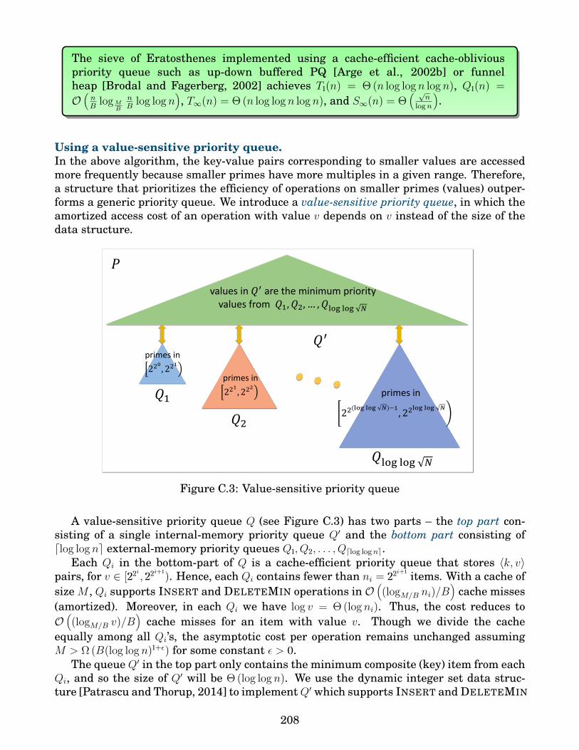
The sieve of Eratosthenes implemented using a cache-efficient cache-obliviouspriority queue such as up-down buffered PQ [Arge et al., 2002b] or funnelheap [Brodal and Fagerberg, 2002] achieves T1(n) = Θ (n log log n log n), Q1(n) =O(nB

log MB

nB

log log n), T∞(n) = Θ (n log log n log n), and S∞(n) = Θ

( √n

logn

).

Using a value-sensitive priority queue.In the above algorithm, the key-value pairs corresponding to smaller values are accessedmore frequently because smaller primes have more multiples in a given range. Therefore,a structure that prioritizes the efficiency of operations on smaller primes (values) outper-forms a generic priority queue. We introduce a value-sensitive priority queue, in which theamortized access cost of an operation with value v depends on v instead of the size of thedata structure.

primes in

220, 221

primes in

221, 222

primes in

22(log log 𝑁)−1, 22log log 𝑁

𝑄1

𝑄2

𝑄log log 𝑁

values in 𝑄′ are the minimum priority values from 𝑄1, 𝑄2, … , 𝑄log log 𝑁

𝑄′

𝑃

Figure C.3: Value-sensitive priority queue

A value-sensitive priority queue Q (see Figure C.3) has two parts – the top part con-sisting of a single internal-memory priority queue Q′ and the bottom part consisting ofdlog log ne external-memory priority queues Q1, Q2, . . . , Qdlog logne.

Each Qi in the bottom-part of Q is a cache-efficient priority queue that stores 〈k, v〉pairs, for v ∈ [22i

, 22i+1). Hence, each Qi contains fewer than ni = 22i+1 items. With a cache ofsize M , Qi supports INSERT and DELETEMIN operations in O

((logM/B ni)/B

)cache misses

(amortized). Moreover, in each Qi we have log v = Θ (log ni). Thus, the cost reduces toO((logM/B v)/B

)cache misses for an item with value v. Though we divide the cache

equally among all Qi’s, the asymptotic cost per operation remains unchanged assumingM > Ω (B(log log n)1+ε) for some constant ε > 0.

The queue Q′ in the top part only contains the minimum composite (key) item from eachQi, and so the size of Q′ will be Θ (log log n). We use the dynamic integer set data struc-ture [Patrascu and Thorup, 2014] to implementQ′ which supports INSERT and DELETEMIN

208

operations on Q′ in O (1) time using only O (log n) space. We also maintain an arrayA[1 : dlog log ne] such that A[i] stores Qi’s contributed item to Q′; thus we can access itin constant time.

To perform a DELETEMIN, we extract the minimum key item from Q′, check its valueto find the Qi it came from, extract the minimum key item from that Qi and insert it intoQ′. To INSERT an item, we first check its value to determine the destination Qi, compareit with the item in A[i], and depending on the result of the comparison we either insert thenew item directly into Qi or move Qi’s current item in Q′ to Qi and insert the new item intoQ′. The following lemma summarizes the performance of these operations.

Complexity analysis of the SE-USING-PQ algorithm

Using a value-sensitive priority queue Q as defined above, an item INSERT withvalue v takes O

(1B

logM/B v)

cache misses, and a DELETEMIN that returns an itemwith value v takes O

(1B

logM/B v)

cache misses, assuming M = Ω (B1+ε) for someconstant ε > 0.

We now use this value-sensitive priority queue to efficiently implement the sieve ofEratosthenes. Each prime p is involved in Θ (n/p) priority queue operations, and by theprime number theorem [Hardy and Wright, 1979], there are O

( √n

logn

)prime numbers in

[1,√n], and the ith prime number is approximately i ln i.

We use the symbol p to denote a prime number. We use the terms sortE(n) (resp.sortI(n)) to denote the per-element I/O cost (resp. internal memory cost) required to sorta set of n numbers. That is sortE(n) = Θ

(1B

logM/BnB

)and from [Han, 2002] sortI(n) =

log log n. The serial cache complexity of the algorithm is computed as

Q1(n) =∑p≤√n

n

p· I/Os for one INSERT or DELETEMIN in Q

=∑p≤√n

n

p· (I/Os for Qi + I/Os for Q′) =

∑p≤√n

n

p· I/Os for Qi =

∑p≤√n

n

p· sortE(p)

= O n

B log MB log logn

∑p≤√n

log pp

= O(

n

B log MB

· lnn)

= O(n

Blog M

Bn)

The total work of the algorithm is computed as

T1(n) =∑p≤√n

n

p· computations for one INSERT or DELETEMIN

=∑p≤√n

n

p· (comp. for Qi + comp. for Q′) =

∑p≤√n

n

p· comp. for Qi +

∑p≤√n

n

p· comp. for Q′

=∑p≤√n

n

p· O (log n) +

∑p≤√n

n

p· sortI(log log n) = O (n log n log log n)

The space complexity of the algorithm is O( √

nlogn

)as we store only the prime numbers

not greater than d√ne.

209

The sieve of Eratosthenes implemented using a cache-efficient cache-obliviousvalue-sensitive priority queue where the Qis are cache-efficient cache-obliviouspriority queues such as up-down buffered PQ [Arge et al., 2002b] or funnelheap [Brodal and Fagerberg, 2002], where M = Ω (log n+B1+ε) for some con-stant ε > 0, achieves T1(n) = Θ (n log log n log n), Q1(n) = O

(nB

log MBn), T∞(n) =

Θ (n log log n log n), and S∞(n) = Θ( √

nlogn

).

Though we reduced the cache complexity the total work increased. We can decreaseboth the cache complexity and the total work using the priority queue of Arge and Tho-rup [Arge and Thorup, 2013], which is simultaneously efficient in RAM and in externalmemory. However, the data structure is cache-aware and is no longer cache-oblivious. Inparticular, their priority queue can handle INSERTs with O

(1B

logM/BnB

)amortized I/Os

and O(logM/B

nB

)amortized RAM operations. DELETEMIN requires O

(1B

logM/BnB

)amor-

tized I/Os and O(logM/B

nB

+ log logM)

amortized RAM operations. They assume that eachelement fits in a machine word and use integer sorting techniques to achieve this low RAMcost while retaining optimal I/O complexity. The total work is computed as

T1(n) =∑p≤√n

n

p· computations for one INSERT or DELETEMIN

=∑p≤√n

n

p· (comp. for Qi + comp. for Q′) =

∑p≤√n

n

p· comp. for Qi +

∑p≤√n

n

p· comp. for Q′

=∑p≤√n

n

p·(sortE(p) + sortI

(M

log log n

))+

∑p≤√n

n

p· sortI(log log n)

= O n

B log MB log logn

∑p≤√n

log pp

+ n · log logM∑p≤√n

1p

+ n · log log log log n∑p≤√n

1p

= O

(n

B log MB

· lnn+ n · (log log log log n+ log logM) · log log n)

= O(n

Blog M

B

n

B+ n log log n · log logM

)

The sieve of Eratosthenes implemented using a cache-efficient cache-aware value-sensitive priority queue where the Qis are cache-efficientcache-aware priority queues of Arge and Thorup [Arge and Thorup,2013], where M = Ω (log n+B(log log n)1+ε) for some constant ε > 0,achieves T1(n) = O

(nB

log MB

nB

+ n log log n · log logM), Q1(n) = O

(nB

log MBn),

T∞(n) = O(nB

log MB

nB

+ n log log n · log logM), and S∞(n) = Θ

( √n

logn

).

C.2 Knapsack problemWe are given a knapsack of capacity W , a set of n unique items, where item i has a value viand weight wi and the item can be used xi number of times. Then, the knapsack problem

210

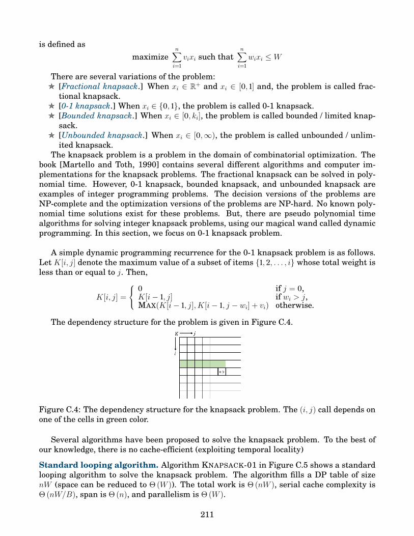
is defined asmaximize

n∑i=1

vixi such thatn∑i=1

wixi ≤ W

There are several variations of the problem:O [Fractional knapsack.] When xi ∈ R+ and xi ∈ [0, 1] and, the problem is called frac-

tional knapsack.O [0-1 knapsack.] When xi ∈ 0, 1, the problem is called 0-1 knapsack.O [Bounded knapsack.] When xi ∈ [0, ki], the problem is called bounded / limited knap-

sack.O [Unbounded knapsack.] When xi ∈ [0,∞), the problem is called unbounded / unlim-

ited knapsack.The knapsack problem is a problem in the domain of combinatorial optimization. The

book [Martello and Toth, 1990] contains several different algorithms and computer im-plementations for the knapsack problems. The fractional knapsack can be solved in poly-nomial time. However, 0-1 knapsack, bounded knapsack, and unbounded knapsack areexamples of integer programming problems. The decision versions of the problems areNP-complete and the optimization versions of the problems are NP-hard. No known poly-nomial time solutions exist for these problems. But, there are pseudo polynomial timealgorithms for solving integer knapsack problems, using our magical wand called dynamicprogramming. In this section, we focus on 0-1 knapsack problem.

A simple dynamic programming recurrence for the 0-1 knapsack problem is as follows.Let K[i, j] denote the maximum value of a subset of items 1, 2, . . . , i whose total weight isless than or equal to j. Then,

K[i, j] =

0 if j = 0,K[i− 1, j] if wi > j,MAX(K[i− 1, j], K[i− 1, j − wi] + vi) otherwise.

The dependency structure for the problem is given in Figure C.4.

Figure C.4: The dependency structure for the knapsack problem. The (i, j) call depends onone of the cells in green color.

Several algorithms have been proposed to solve the knapsack problem. To the best ofour knowledge, there is no cache-efficient (exploiting temporal locality)

Standard looping algorithm. Algorithm KNAPSACK-01 in Figure C.5 shows a standardlooping algorithm to solve the knapsack problem. The algorithm fills a DP table of sizenW (space can be reduced to Θ (W )). The total work is Θ (nW ), serial cache complexity isΘ (nW/B), span is Θ (n), and parallelism is Θ (W ).

211

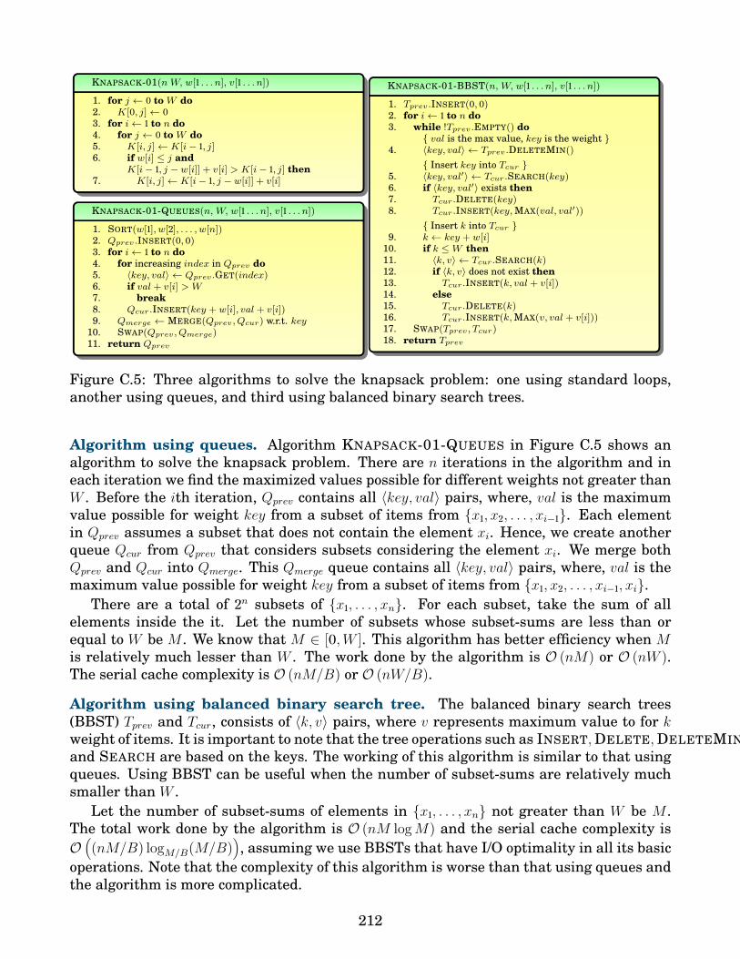
KNAPSACK-01(n W, w[1 . . . n], v[1 . . . n])

1. for j ← 0 to W do2. K[0, j]← 03. for i← 1 to n do4. for j ← 0 to W do5. K[i, j]← K[i− 1, j]6. if w[i] ≤ j and

K[i− 1, j − w[i]] + v[i] > K[i− 1, j] then7. K[i, j]← K[i− 1, j − w[i]] + v[i]

KNAPSACK-01-QUEUES(n, W, w[1 . . . n], v[1 . . . n])

1. SORT(w[1], w[2], . . . , w[n])2. Qprev .INSERT(0, 0)3. for i← 1 to n do4. for increasing index in Qprev do5. 〈key, val〉 ← Qprev .GET(index)6. if val + v[i] > W7. break8. Qcur.INSERT(key + w[i], val + v[i])9. Qmerge ← MERGE(Qprev , Qcur) w.r.t. key

10. SWAP(Qprev , Qmerge)11. return Qprev

KNAPSACK-01-BBST(n, W, w[1 . . . n], v[1 . . . n])

1. Tprev .INSERT(0, 0)2. for i← 1 to n do3. while !Tprev .EMPTY() do

val is the max value, key is the weight 4. 〈key, val〉 ← Tprev .DELETEMIN()

Insert key into Tcur 5. 〈key, val′〉 ← Tcur.SEARCH(key)6. if 〈key, val′〉 exists then7. Tcur.DELETE(key)8. Tcur.INSERT(key,MAX(val, val′))

Insert k into Tcur 9. k ← key + w[i]

10. if k ≤W then11. 〈k, v〉 ← Tcur.SEARCH(k)12. if 〈k, v〉 does not exist then13. Tcur.INSERT(k, val + v[i])14. else15. Tcur.DELETE(k)16. Tcur.INSERT(k,MAX(v, val + v[i]))17. SWAP(Tprev , Tcur)18. return Tprev

Figure C.5: Three algorithms to solve the knapsack problem: one using standard loops,another using queues, and third using balanced binary search trees.

Algorithm using queues. Algorithm KNAPSACK-01-QUEUES in Figure C.5 shows analgorithm to solve the knapsack problem. There are n iterations in the algorithm and ineach iteration we find the maximized values possible for different weights not greater thanW . Before the ith iteration, Qprev contains all 〈key, val〉 pairs, where, val is the maximumvalue possible for weight key from a subset of items from x1, x2, . . . , xi−1. Each elementin Qprev assumes a subset that does not contain the element xi. Hence, we create anotherqueue Qcur from Qprev that considers subsets considering the element xi. We merge bothQprev and Qcur into Qmerge. This Qmerge queue contains all 〈key, val〉 pairs, where, val is themaximum value possible for weight key from a subset of items from x1, x2, . . . , xi−1, xi.

There are a total of 2n subsets of x1, . . . , xn. For each subset, take the sum of allelements inside the it. Let the number of subsets whose subset-sums are less than orequal to W be M . We know that M ∈ [0,W ]. This algorithm has better efficiency when Mis relatively much lesser than W . The work done by the algorithm is O (nM) or O (nW ).The serial cache complexity is O (nM/B) or O (nW/B).

Algorithm using balanced binary search tree. The balanced binary search trees(BBST) Tprev and Tcur, consists of 〈k, v〉 pairs, where v represents maximum value to for kweight of items. It is important to note that the tree operations such as INSERT,DELETE,DELETEMIN,and SEARCH are based on the keys. The working of this algorithm is similar to that usingqueues. Using BBST can be useful when the number of subset-sums are relatively muchsmaller than W .

Let the number of subset-sums of elements in x1, . . . , xn not greater than W be M .The total work done by the algorithm is O (nM logM) and the serial cache complexity isO((nM/B) logM/B(M/B)

), assuming we use BBSTs that have I/O optimality in all its basic

operations. Note that the complexity of this algorithm is worse than that using queues andthe algorithm is more complicated.

212

Tiled iterative algorithmWe assume that the weights are sorted. The entire DP table (of size nW ) is divided into(n/n′)×(W/n′) chunks each of size (n′×n′), as shown in Figure C.6. We define two functions:A(X,X) that both reads and writes to the same chunk X, and B(X,U) that reads fromchunk U and writes to a different region X, where X , U . The order of function calls(timestamps) for a grid (of chunks) of size 4× 6 is shown in Figure C.7. The subscripts forthe functions represent the timesteps at which a function can update a particular region.

𝑛′

𝑊

𝑛

𝑤𝑛

𝑤𝑖

𝑤1

𝑛′

Figure C.6: Division of the DP table into chunks.

TILED-KNAPSACK()

1. for i← 1 to n/n′ do2. for j ← 1 to W/n′ do3. U ← chunk[i, j]; A(U,U)4. for k ← 1 to n′ do5. pos← (w(j−1)×n′+k)/n′6. X ← chunk[i, j + pos]; B(X,U)7. X ← chunk[i, j + pos+ 1]; B(X,U)

𝐴0 𝐵1𝐴2 𝐵1𝐵3𝐴4 𝐵1𝐵3𝐵5𝐴6 𝐵1𝐵3𝐵5𝐵7𝐴8 𝐵1𝐵3𝐵5𝐵7𝐵9𝐴10




Figure C.7: Tiled knapsack algorithm.

The complexity of the tiled algorithm is given in Theorem 17.

Theorem 17 (Complexity of TILED-KNAPSACK). The cache-aware processor-aware algorithm achieves T1(n) = Θ (nW ), Q1(n) = O

(nWB

+ n), and Sp(n) =

Θ (pWn′), where p is the number of processors.

Proof. We prove the theorem in several parts.Work. We will not write recurrence relations to compute the work. This is because thenumber of function calls invoked at every level varies as a function call F(X,U), whereF ∈ A,B is invoked only if there is a dependency of any cell from X region to U region.Hence, we use a different technique to compute the total work.

Consider Figure C.6. We define something called a dependency curve. It is the cells onthe path of the red curve shown in the figure on which the cells in the last column of theDP table depends on. It is simply the graph of the increasing order of weights shown fromthe rightmost column. Every column of blocks will have a dependency curve too. In total,there can be at most O (nW/(n′)2) number of function calls.

213

Every cell (i, j) in the DP table depends on cell (i − 1, j). Therefore, every chunk (I, J)depends on itself, which requires an A function invocation. Hence, the total number of Afunction calls will be (n/n′)× (W/n′) = nW/(n′)2.

A cell (i, j) depends on the cell (i − 1, j − wi) if j ≥ wi. Let the cell (i, j) be present inchunk (I, J) and the cell (i − 1, j − wi) be present in chunk (I, J ′), where J ′ ≤ J − 1. Then,a B function will be executed that writes to chunk (I, J) reading from chunk (I, J ′), whereJ ′ ≤ J − 1. As we will never call a B function twice, that writes to a chunk X and readsfrom a chunk U , the total number of B calls will be Θ ((n/n′)× (W/n′)) = Θ (nW/(n′)2).

The total work is the product of the number of function calls to A and B and the workdone by those functions. That is, the total work is Θ (nW/(n′)2)×Θ ((n′)2) = Θ (nW ).Space complexity. In the serial case, we process the n′ × n′ chunks present in single rowof chunks. Hence, the serial space complexity is Θ (nn′). In the parallel version with pprocessors, we run at most p rows of chunks. Hence, the parallel space complexity will beΘ (pWn′).Serial cache complexity. Temporal locality can be exploited as long as the work is asymp-totically greater than the space. The B function takes O ((n′)2) space and does O ((n′)2). AsB function is invoked a total of O (nW/(n′)2) times it is a dominating function. Hence, therecannot be any temporal locality. So, the serial cache complexity is O (nW/B).

Divide-and-conquer wavefront (WR-DP) algorithmPlease refer Chapter 3 for a comprehensive introduction and analysis to divide-and-conquerwavefront algorithms. Algorithm RECURSIVE-WAVEFRONT-KNAPSACK in Figure C.8 givesa WR-DP algorithm for the knapsack problem. A diagrammatic representation of thedivide-and-conquer algorithm is given in Figure C.9. It is assumed that before calling ourdivide-and-conquer algorithm, we would have a sorted list of item weights.

Suppose f ∈ A,B and f(X,U) be a function call. It is important to note that f will beinvoked if and only if DEPENDS(X,U) is true i.e., there is some cell in X that depends onsome cell in U .

Completion-time is found from the DP recurrence:

C(i, j) =

0 if i = 0 and j = 0,C(i, j − 1) + 2 if j > 0,C(i− 1, j) + 2 if i > 0.

The start- and end-time functions are computed as follows.

SA (X,X) = EA (X,X) = C(xr, xc) if X is a n′ × n′ chunk,SA (X,X) = SA (X11, X11) if X is not a n′ × n′ chunk,EA (X,X) = EA (X22, X22) if X is not a n′ × n′ chunk,SB (X,U) = EB (X,U) = C(ur, uc) + 1 if X is a n′ × n′ chunk,SB (X,U) = SB (X11, U11) if X is not a n′ × n′ chunk,EB (X,U) = EB (X22, U22) if X is not a n′ × n′ chunk.

Solving the recurrences, we have

214

RECURSIVE-WAVEFRONT-KNAPSACK()

1. w ← 02. while w <∞ do w ← A(G,G,w)

A(X,X,w)

1. vi ←∞ for all i ∈ [1, 6]2. if X is an n′ × n′ matrix then3. if w = SA (X,X) then Achunk(X,X)4. else5. F1..6 ← A,B,A,A,B,A6. arg1..6 ← (X11, X11), (X12, X11), (X12, X12),

(X21, X21), (X22, X21), (X22, X22)7. parallel for i← 1 to 6 do8. if DEPENDS(argi) then9. if w < SFi




C(i, j)

1. return 2(i+ j)

SA (X,X)

1. return C(xr, xc)

SB (X,U)

1. return C(ur, uc) + 1

B(X,U,w)

1. vi ←∞ for all i ∈ [1, 8]2. if X is an n′ × n′ matrix then3. if w = SB (X,U) then Bchunk(X,U)4. else5. F1..8 ← B,B,B,B,B,B,B,B6. arg1..8 ← (X11, U11), (X12, U11), (X21, U21),

(X22, U21), (X11, U12), (X12, U12),(X21, U22), (X22, U22)

7. parallel for i← 1 to 8 do8. if DEPENDS(argi) then9. if w < SFi




DEPENDS(X,U)

1. if some cell(s) in X depends on some cell(s) in U then2. return true3. else return false

EA (X,X)


EB (X,U)

1. return C(ur + n− n′, uc + n− n′) + 1

Figure C.8: A recursive divide-and-conquer wavefront DP algorithm for the knapsack prob-lem. A region Z has its top-left corner at (zr, zc) and is of size n× n.

C(i, j) = 2(i+ j)SA (X,X) = C(xr, xc); EA (X,X) = C(xr + n− n′, xc + n− n′)SB (X,U) = C(ur, uc) + 1; EB (X,U) = C(ur + n− n′, uc + n− n′) + 1

Theorem 18 (Complexity of RECURSIVE-WAVEFRONT-KNAPSACK). The cache-aware processor-aware algorithm achieves T1(n) = Θ (nW ), Q1(n) = O

(nWB

+ n), and

Sp(n) = Θ (pWn′), where p is the number of processors.

Proof. The proof is similar to that of Theorem 17.

Sliding window algorithmLet w1, . . . , wn be sorted in increasing order and let wn = f(M), where f(M) = o (M). Thesliding window algorithm is given in Figure C.10. Let ` = 1. Let array output[0 . . .W ]represent the 0th row of the knapsack DP table. We find the maximum value of h suchthat w` + w`+1 + · · · + wh ≤ γM , for some constant γ. Then using w` + w`+1 + · · · + wh spaceinside RAM, we can compute the rows ` . . . h of the DP table and output the hth row of theknapsack DP table to the external-memory. We repeat the process by setting ` = h+ 1 andreading again from the array output[0 . . .W ].

215

Figure C.9: A recursive divide-and-conquer DP algorithm for the knapsack problem.

Theorem 19 (Complexity of SLIDING-WINDOW-KNAPSACK). The cache-awarealgorithm achieves T1(n) = Θ (nW ), Q1(n) = Θ

(wcount ·

(WB

+ 1))

, where wcount =

O(

n

( Mf(M))

), and S1(n) = O

(WB

).

Proof. Only the required computations are performed by the algorithm and no extra com-putations are done. Hence, the work remains Θ (nW ). At any time, the we use only con-stant number of rows of the knapsack DP table. Hence, the space used is Θ (W/B). Wesee that at a time (or any particular iteration), a bunch of ω (1) rows are computed in RAMand the array is written to the external memory for that bunch only once. Every time wewrite / overwrite a row to the disk, we increment the wcount (meaning write counter) by 1.Hence, the total number of times we write a row is wcount. Hence, the total serial cachecomplexity is Θ (wcount · ((W/B) + 1)). We know that wcount = o (n/ω (1)) and hence weexploit temporal locality and the algorithm is cache-efficient.

216

SLIDING-WINDOW-KNAPSACK()

1. `← 12. output[0 . . .W ]← ∅3. wcount← 14. while ` < n do5. Find largest h such that

∑h

i=`wi ≤M

6. Read the data from output[0 . . .W ]7. Compute the rows ` . . . h of the knapsack DP

table8. Write output to output array9. wcount← wcount+ 1

10. `← h+ 1

0 1 2 3 4 5 6 7 8 9 10 11 12 13 14 15 16 17

0 0 0 0 0 0 0 0 0 0 0 0 0 0 0 0 0 0 0

2 0 0 1 0 0 0 0 0 0 0 0 0 0 0 0 0 0 0

3 0 0 1 1 0 1 0 0 0 0 0 0 0 0 0 0 0 0

5 0 0 1 1 0 1 0 1 1 0 1 0 0 0 0 0 0 0

7 0 0 1 1 0 1 0 1 1 1 1 0 1 0 1 1 0 1

10 0 0 1 1 0 1 0 1 1 1 1 0 1 1 1 1 0 1

0 1 2 3 4 5 6 7 8 9 10 11 12 13 14 15 16 17

0 0 0 0 0 0 0 0 0 0 0 0 0 0 0 0 0 0 0

2 0 0 1 0 0 0 0 0 0 0 0 0 0 0 0 0 0 0

3 0 0 1 1 0 1 0 0 0 0 0 0 0 0 0 0 0 0

5 0 0 1 1 0 1 0 1 1 0 1 0 0 0 0 0 0 0

7 0 0 1 1 0 1 0 1 1 1 1 0 1 0 1 1 0 1

10 0 0 1 1 0 1 0 1 1 1 1 0 1 1 1 1 0 1

𝑤𝑙

𝑊

𝑤ℎ

Figure C.10: Sliding window knapsack algorithm. Left: The pseudocode. Right: An exam-ple of subset sum problem.

Sliding merging window algorithmThis algorithm has similarities to the sliding window knapsack algorithm. Let w1, . . . , wnbe sorted in increasing order. Let si represent the maximum number of subset sums (usingweights w1, . . . , wi) in the range [a, a + wi], for all a ∈ [0,W − wi]. Let sn = f(M), wheref(M) = o (M).

Let ` = 1. Let array output[0 . . .W ] represent the 0th row of the knapsack DP table. Wefind the maximum value of h such that m` + m`+1 + · · · + mh ≤ γM , for some constant γ.Then using m`+m`+1+ · · ·+mh space inside RAM, we can compute the rows ` . . . h of the DPtable and output the hth row of the knapsack DP table to the external-memory. We repeatthe process by setting ` = h+ 1 and reading again from the array output[0 . . .W ].

Computing si. How can we find si? We can compute si using the formula si = (wi/di),where di can be found by solving the integer programming problem. Let

∑ij=1 xjwj = di,

where di ∈ [1, w1] and di is minimum possible value, and xj ∈ −1, 0, 1. The integer pro-gramming problem might be hard to solve in polynomial time. But, probably there existconstant factor approximation algorithms.

Variants of the problemThe Knapsack problem is similar to the change making problem and the subset-sum prob-lem. All these problems have data-sensitive dependency. That is, the DP dependencystructure for the problem is dependent on each run / execution of the algorithm.

Change making problem. We have n coins of denominations c1, c2, . . . , cn. We need tomake a change for m amounts of money in minimum number of coins. We need to find thenumber of coins of each denomination that makes a change for m. There are four versionsof the problem.

217

O Greedy algorithm when there are unlimited number of coins of each denomination.See Figure C.11.

O DP algorithm when there are unlimited number of coins of each denomination. SeeFigure C.11.

O DP algorithm when there is exactly 1 coin of each denomination. The problem is alsocalled as 01 change making problem. See Figure C.11.

O DP algorithm when there are limited number of coins of each denomination, sayk1, k2, . . . , kn. See Figure C.11.

Subset-sum problem. In this problem, we are given a multiset S = x1, x2, . . . , xn of nintegers. We set P [i, j] to true if a subset of x1, x2, . . . , xi sums to j, and to false otherwise.Then,

P [i, j] =

true if j = 0,true if P [i− 1, j] = true or P [i− 1, j − xi] = true,false otherwise.

218

CM-UNLIMITED-GREEDY(n m, c[1 . . . n])

Require: c[1] > c[2] > · · · > c[n]1. money ← m2. for i← 1 to n do3. a[i]←

⌊money

c[i]

⌋4. mc← mc+ a[i]5. money ← money − a[i]c[i]6. if money > 0 then7. print Cannot make change8. else return a[1 . . . n], mc

CM-UNLIMITED-DP(n m, c[1 . . . n])

Compute the minimum number of coins 1. mc[0]← 02. for i← 1 to m do3. mc[i]←∞4. for j ← 1 to n do5. if c[j] ≤ i and mc[i− c[j]] + 1 < mc[i] then6. mc[i]← mc[i− c[j]] + 1; parent[i]← j

Compute #coins of each denomination 7. if mc[m] =∞ then print Cannot make change8. else9. a[1 . . . n]← ∅; i← m

10. while i ≥ 1 do11. a[parent[i]]← a[parent[i]] + 1; i← i− c[parent[i]]12. return a[1 . . . n], mc[m]

CM-LIMITED-01-DP(n m, c[1 . . . n])

Compute the minimum number of coins 1. mc[0, 0 . . .m]←∞; mc[0 . . . n, 0]← ∅2. for i← 1 to n do3. for j ← 1 to m do4. mc[i, j]← mc[i− 1, j]; parent[i, j]← 05. if c[i] ≤ j and mc[i− 1, j− c[i]]+ 1 < mc[i, j] then6. mc[i, j]← mc[i, j − c[i]] + 1; parent[i, j]← 1 Compute #coins of each denomination

7. if mc[n,m] =∞ then print Cannot make change8. else9. a[1 . . . n]← ∅; j ← m

10. for i← n to 1 do11. if parent[i, j] = 1 then12. j = j − c[i]; a[i]← a[i] + 113. return a[1 . . . n], mc[n,m]

CM-LIMITED-DP(n, m, c[1 . . . n], k[1 . . . n])

Input: n number of denominations, m money to bechanged for, c[1 . . . n] coin denominations, k[1 . . . n]number of coins availableOutput: a[1 . . . n] number of coins used,mincoins[nn][mm] minimum number of coinsRequire: a[1] + a[2] + · · ·+ a[n] is minimized Convert the limited change making problem to 0-1

change making problem 1. mm← m; nn← 02. for i← 1 to n do3. if k[i] > 0 then4. count← 0; power ← 15. repeat6. if count+ power > k[i] then7. power ← k[i]− count8. nn← nn+ 19. cc[nn]← power × c[i]

10. d[nn]← i;11. v[nn]← power12. count← count+ power13. power ← 2× power14. until count = k[i] Compute the minimum number of coins

15. mincoins[0 . . . nn][0]← ∅16. mincoins[0][0 . . . nn]← ∅17. for i← 1 to nn do18. for j ← 1 to mm do19. mincoins[i][j]← mincoins[i− 1][j]20. parent[i][j]← 021. if cc[i] ≤ j and mincoins[i − 1][j − cc[i]] + v[i] <

mincoins[i][j] then22. mincoins[i][j]← mincoins[i− 1][j − cc[i]] + v[i]23. parent[i][j]← 1 Compute #coins of each denomination

24. if mincoins[nn][mm] =∞ then25. print Cannot make change26. else27. a[1 . . . nn]← ∅; j ← mm28. for i← nn to 1 do29. if parent[i][j] = 1 then30. j ← j − cc[i]31. a[d[i]]← a[d[i]] + v[i]32. return a[1 . . . n], mincoins[nn][mm]

Figure C.11: Change making algorithms.

219

Appendix D

Efficient Divide-&-Conquer Tiled DPAlgorithms

In this section, we present new r-way R-DP algorithms for several DP problems. Suchalgorithms can be easily converted to cache-aware tiled algorithms by following the processas described in Section 3.2.

D.1 Matrix multiplicationThough MM is not a DP problem, the approach followed to get a 2-way divide-and-conqueralgorithm is similar as for a DP problem. A 2-way divide-and-conquer algorithm for MMwas presented in [Frigo et al., 1999]. It is extremely easy to generalize it to an r-waydivide-and-conquer algorithm and it is presented in Figure D.1.

AMM (X,U, V, d)

1. r ← tilesize[d]2. if r ≥ m then Aloop-MM (X,U, V )

else3. for k ← 1 to r do4. parallel: AMM (Xij , Uik, Vkj , d+ 1) for i, j ∈ [1, r]

Figure D.1: An r-way R-DP for matrix multiplication.

D.2 Longest common subsequenceThe problem is described in detail in Section A.1. An r-way R-DP to solve the problem isgiven in Figure D.2.

D.3 Floyd-Warshall’s all-pairs shortest pathThe problem is described in detail in Section A.3. An r-way R-DP algorithm for Floyd-Warshall’s APSP is described in Figure A.7.

220

ALCS(X, d)

1. r ← tilesize[d]2. if r ≥ m then Aloop-LCS(X)

else3. for k ← 0 to 2r − 2 do4. parallel: ALCS(Xij , d+ 1) for i ∈ [max(1, k − r + 2),min(k + 1, r)] and j = k − i+ 2

Figure D.2: An r-way R-DP for LCS.

D.4 Gaussian elimination without pivotingThe problem is described in detail in Section A.4. An r-way R-DP algorithm for Gaussianelimination without pivoting is given in Figure D.3.

AGE(X,U, V,W, d)

1. r ← tilesize[d]2. if r ≥ m then Aloop-GE(X,U, V,W )

else3. for k ← 1 to r do4. AGE(Xkk, Ukk, Vkk,Wk, d+ 1)5. parallel: BGE(Xkj , Ukk, Vkj ,Wk, d+ 1), CGE(Xik, Uik, Vkk,Wk, d+ 1) for i, j ∈ [k + 1, r]6. parallel: DGE(Xij , Uik, Vkj ,Wk, d+ 1) for i, j ∈ [k + 1, r]

BGE(X,U, V,W, d)

1. r ← tilesize[d]2. if r ≥ m then Bloop-GE(X,U, V,W )

else3. for k ← 1 to r do4. parallel: BGE(Xkj , Ukk, Vkj ,Wk, d+ 1) for j ∈ [1, r]5. parallel: DGE(Xij , Uik, Vkj ,Wk, d+ 1) for i ∈ [k + 1, r], j ∈ [1, r]

CGE(X,U, V,W, d)

1. r ← tilesize[d]2. if r ≥ m then Cloop-GE(X,U, V,W )

else3. for k ← 1 to r do4. parallel: CGE(Xik, Uik, Vkk,Wk, d+ 1) for i ∈ [1, r]5. parallel: DGE(Xij , Uik, Vkj ,Wk, d+ 1) for i ∈ [1, r], j ∈ [k + 1, r]

DGE(X,U, V,W, d)

1. r ← tilesize[d]2. if r ≥ m then Dloop-GE(X,U, V,W )

else3. for k ← 1 to r do4. parallel: DGE(Xij , Uik, Vkj ,Wk, d+ 1) for i, j ∈ [1, r]

Figure D.3: An r-way R-DP for Gaussian elimination without pivoting algorithm.

D.5 Parenthesis problemThe problem is described in detail in Section A.2. An r-wayR-DP was presented in [Chowd-hury and Ramachandran, 2008] and its complete pseudocode is given in Figure D.4.

221

Apar(X,U, V, d)

1. r ← tilesize[d]2. if r ≥ m then Aloop-par(X,U, V )

else3. Let diagonal represent (j − i)4. parallel: Apar(Xi,j , Ui,j , Vi,j , d+ 1) for i, j ∈ [1, r] and diagonal = 05. for k ← 1 to r − 1 do6. parallel: Cpar(Xi,j , Ui,k+i−1, Vk+i−1,j , d+ 1) for i, j ∈ [1, r] and diagonal ∈ [k,min2k − 2, r − 1]7. parallel: Cpar(Xi,j , Ui,1+i, V1+i,j , d+ 1) for i, j ∈ [1, r] and diagonal ∈ [k,min2k − 3, r − 1]8. parallel: Bpar(Xi,j , Ui,i, Vj,j , d+ 1) for i, j ∈ [1, r] and diagonal = k

Bpar(X,U, V, d)

1. r ← tilesize[d]2. if r ≥ m then Bloop-par(X,U, V )

else

3. Let U ′i,` =Xi,` if ` > 0,Ui,`+r if ` ≤ 0.

and V ′`,j =V`,j if ` > 0,X`+r,j if ` ≤ 0.

4. Let diagonal represent (j − i)5. for k ← 1 to 2r − 1 do6. parallel: Cpar(Xi,j , U

′i,k−r+i−1, V

′k−r+i−1,j , d+ 1) for i, j ∈ [1, r] and diagonal + r ∈ [k,min2k − 2, 2r − 1]

7. parallel: Cpar(Xi,j , U′i,1+i−r, V

′1+i−r,j , d+ 1) for i, j ∈ [1, r] and diagonal + r ∈ [k,min2k − 3, 2r − 1]

8. parallel: Bpar(Xi,j , Ui,i, Vj,j , d+ 1) for i, j ∈ [1, r] and diagonal + r = k

Cpar(X,U, V, d)

1. r ← tilesize[d]2. if r ≥ m then Cloop-par(X,U, V )

else3. for k ← 1 to r do4. parallel: Cpar(Xi,j , Ui,k, Vk,j , d+ 1) for i, j ∈ [1, r]

Figure D.4: An r-way R-DP for parenthesis problem.

D.6 Sequence alignment with gap penaltyThe problem is described in detail in Section A.5. An r-way R-DP to solve the problem isgiven in Figure D.5.

222

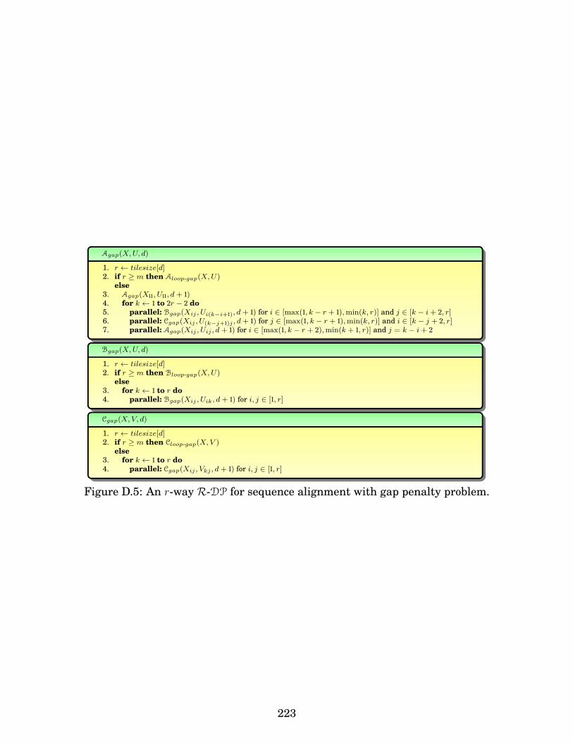
Agap(X,U, d)

1. r ← tilesize[d]2. if r ≥ m then Aloop-gap(X,U)

else3. Agap(X11, U11, d+ 1)4. for k ← 1 to 2r − 2 do5. parallel: Bgap(Xij , Ui(k−i+1), d+ 1) for i ∈ [max(1, k − r + 1),min(k, r)] and j ∈ [k − i+ 2, r]6. parallel: Cgap(Xij , U(k−j+1)j , d+ 1) for j ∈ [max(1, k − r + 1),min(k, r)] and i ∈ [k − j + 2, r]7. parallel: Agap(Xij , Uij , d+ 1) for i ∈ [max(1, k − r + 2),min(k + 1, r)] and j = k − i+ 2

Bgap(X,U, d)

1. r ← tilesize[d]2. if r ≥ m then Bloop-gap(X,U)

else3. for k ← 1 to r do4. parallel: Bgap(Xij , Uik, d+ 1) for i, j ∈ [1, r]

Cgap(X,V, d)

1. r ← tilesize[d]2. if r ≥ m then Cloop-gap(X,V )

else3. for k ← 1 to r do4. parallel: Cgap(Xij , Vkj , d+ 1) for i, j ∈ [1, r]

Figure D.5: An r-way R-DP for sequence alignment with gap penalty problem.

223

Appendix E

Efficient Divide-&-Conquer Hybrid DPAlgorithms

In this section, we develop hybrid divide-and-conquer algorithms for three problems: multi-instance Viterbi algorithm, Floyd-Warshall’s all-pairs shortest path, and protein accordionfolding.

E.1 Matrix multiplicationComplexities for Lemma 3 is shown below.

Q1(n) = 8Q1

(n

2

)+ c = 8

(Q1

(n

22)

+ c)

+ c = 82Q1

(n

22)

+ c(81 + 80

)= 8kQ1

(n

2k)

+ c(8k−1 + · · ·+ 80

)≤ 8kc′

(M

B+√M)

+ c8k

≤ 8log4n2M c′

(M

B+√M)

+ c8log4n2M

(∵ (n/2k)2 ≤ αM

)= O

(n3

B√M

+ n3

M√M

+ n3

M+ n2

B+ n

)

= O(

n3

B√M

+ n2

B+ n

) (∵M = Ω

(B2))

Sp(m) = 8Sp(m

2

)+ cm2 = 82Sp

(m

22)

+ cm2( 822

+ 1)

= 8kSp(m

2k)

+ cm2(

8k−1

(2k−1)2 + · · ·+ 1)

≤ 8kSp(m

2k)

+ cm22k(Say (2k)3 ≤ p

)≤ 8log8 p ·Θ

((n

2log8 p

)2)

+ cn22log8 p = Θ(n2p1/3

)(Set m = n)

The detailed derivation of the complexities of Theorem 13 is given here.

T1(n) = 8T1

(n

2

)+ c = 8

(8T1

(n

22)

+ c)

+ c = 82T1

(n

22)

+ c(81 + 1

)= 8kT1

(n

2k)

+ c(8k−1 + · · ·+ 1

)≤ 8kc′

(n

2k)3

+ 8kc = O(n3)

224

Q1(n) = 8Q1

(n

2

)+ c = 8

(Q1

(n

22)

+ c)

+ c = 82Q1

(n

22)

+ c(81 + 80

)= 8kQ1

(n

2k)

+ c(8k−1 + · · ·+ 80

)≤ 8kc′

((n

2k)3 1B√M

)+ c8k

≤ c′n3

B√M

+ c8log4n2M = O

(n3

B√M

+ n2

B+ n

)

T∞(n) = T∞

(n

2

)+ c log n = T∞

(n

22)

+ c(

log n+ log n2

)= T∞

(n

2k)

+ c(

log n+ · · ·+ log n

2k−1)

= c′n

2k+ c

((k − 1) log n− (k − 1)k

2

)= O

(n

2k+ k(2 log n− k)

)

E.2 Multi-instance Viterbi algorithmA multi-instance Viterbi algorithm is described in Section 4.3. An in-place divide-and-conquer algorithm is given in . The AV A function in the algorithm will be called Θ (t) timesand the function is similar in recursive structure to AMM of Figure 6.3. In this Viterbiproblem, there is only one recursive function AV A and it is MM-like. Hence, it satisfies thespan property (Theorem 12) and we can replace it with its not-in-place / hybrid version ofthe function.

Lemma 4 (In-place VA). The in-place VA Multi-Instance-Viterbi, assuming a tallcache, has a complexity of T1(n) = Θ (n3t), Q1(n) = Θ

(n3t/(B

√M) + n2t/B + nt

),

T∞(n) = Θ (nt), and Sp(n) = Θ (n2).

Proof. The recurrences for the complexities of AV A is exactly the same as that in Lemma2. Also, the function AV A is invoked t times as there are t timesteps. Hence, the lemmafollows.

Following the argument of Lemma 4 and recurrences from Lemma 3, we can proveLemma 5. Similarly, following the argument of Lemma 4 and recurrences from Theorem13, we can prove Theorem 20.

Lemma 5 (Not-in-place VA). The not-in-place multi-instance Viterbi algo-rithm, assuming a tall cache, has a complexity of T1(n) = Θ (n3t), Q1(n) =Θ(n3t/(B

√M) + n2t/B + nt

), T∞(n) = Θ

(t log2 n

), and Sp(n) = Θ

(p1/3n2

).

Theorem 20 (Hybrid VA). The hybrid multi-instance Viterbi algorithm, as-suming a tall cache, has a complexity of T1(n) = Θ (n3t), Q1(n) =O(n3t/(B

√M) + n2t/B + nt

), T∞(n) = O

(kt(2 log n− k) + nt/2k

), and Sp(n) =

O(minp1/3, 2kn2

).

225

E.3 Floyd-Warshall’s all-pairs shortest pathFloyd-Warshall’s all-pairs shortest path algorithm is described in Section A.3. FiguresA.5 and A.6 show an in-place 2-way divide-and-conquer algorithm. The D function in thealgorithm is matrix-multiplication-like and dominates the total work complexity. Hence,by simply modifying the D function to use extra space, we end up with not-in-place FWalgorithm.

Lemma 6 (In-place FW). The in-place FW, assuming a tall cache, has a complex-ity of T1(n) = Θ (n3), Q1(n) = Θ

(n3/(B

√M) + n2/B + n

), T∞(n) = Θ

(n log2 n

), and

Sp(n) = Θ (n2).

Proof. The recurrences are as follows. For f ∈ A,B,C,D, let Qf (n) and Tf (n) denote theserial cache complexity and span of fFW on a matrix of size n× n. Then

QA(n) = QB(n) = QC(n) = QD(n) = O(n2

B+ n

)if n2 ≤ γM ,

QA(n) = 2(QA

(n

2

)+QB

(n

2

)+QC

(n

2

)+QD

(n

2

))+ Θ (1) if n2 > γAM .

QB(n) = 4(QB

(n

2

)+QD

(n

2

))+ Θ (1) if n2 > γBM .

QC(n) = 4(QC

(n

2

)+QD

(n

2

))+ Θ (1) if n2 > γCM .

QD(n) = 8QD

(n

2

)+ Θ (1) if n2 > γDM .

TA(n) = TB(n) = TC(n) = TD(n) = O (1) if n = 1,

TA(n) = 2(TA

(n

2

)+ + max TB

(n

2

), TC

(n

2

)+ TD

(n

2

))+ Θ (1) if n > 1.

TB(n) = 2(TB

(n

2

)+ TD

(n

2

))+ Θ (1) if n > 1.

TC(n) = 2(TC

(n

2

)+ TD

(n

2

))+ Θ (1) if n > 1.

TD(n) = 2TD(n

2

)+ Θ (1) if n > 1.

where, γ, γA, γB, γC and γD are suitable constants, Q1(n) = QA(n), and T∞(n) = TA(n).Solving, we have the lemma.

Lemma 7 (Not-in-place FW). The not-in-place FW, assuming a tall cache, has acomplexity of T1(n) = Θ (n3), Q1(n) = Θ

(n3/(B

√M) + n2/B + n

), T∞(n) = Θ (n log n),

and Sp(n) = Θ(p1/3n2

).

Proof. The recurrences from Lemma 6 will be the same except the following.

TD(n) = TD

(n

2

)+ Θ (log n) if n > 1.

Solving the recurrences, the lemma follows.

The recurrences for the hybrid algorithm are:

226

QA(m) = QB(m) = QC(m) = QD(m) = O(

(n/2k)3

B√M

+ (n/2k)2B

+ (n/2k))

if m = n

2k,

QA(m) = 2(QA

(m

2

)+QB

(m

2

)+QC

(m

2

)+QD

(m

2

))+ Θ (1) if m >

n

2k.

QB(m) = 4(QB

(m

2

)+QD

(m

2

))+ Θ (1) if m >

n

2k.

QC(m) = 4(QC

(m

2

)+QD

(m

2

))+ Θ (1) if m >

n

2k.

QD(m) = 8QD

(m

2

)+ Θ (1) if m >

n

2k.

TA(m) = Θ((n/2k) log2(n/2k)

)if m = n/2k,

TB(m) = TC(m) = Θ((n/2k) log(n/2k)

)if m = n/2k,

TD(m) = Θ(n/2k

)if m = n/2k,

TA(m) = 2(TA

(m

2

)+ max TB

(m

2

), TC

(m

2

)+ TD

(m

2

))+ Θ (logm) if m > n/2k.

TB(m) = 2(TB

(m

2

)+ TD

(m

2


TC(m) = 2(TC

(m

2

)+ TD

(m

2


TD(m) = TD

(m

2

)+ Θ (logm) if m > n/2k.

Sp(n) = minp1/3, n2k−1∑i=0

8i(n

2i× n

2i) = Θ

(minp1/3, 2kn2

)Derivation of the cache complexity is given here.

QD(n) = 8QD

(n

2

)+ c = 8

(8QD

(n

22)

+ c)

+ c

= 82QD

(n

22)

+ c(81 + 80

)= 8kQD

(n

2k)

+ c(8k−1 + 8k−2 + · · ·+ 80

)≤ 8kc′

((n/2k)3

B√M

)+ c8k = O

(n3

B√M

)It is important to note that

QD

(n

2i)

= O(

(n/2i)3

B√M

)

QC(n) = 4QC

(n

2

)+ 4QD

(n

2

)+ c = 4

(4QC

(n

22)

+ 4QD

(n

22)

+ c)

+ 4QD

(n

2

)+ c

= 42QC

(n

22)

+ 42QD

(n

22)

+ 4QD

(n

2

)+ c

(41 + 40

)= 4kQC

(n

2k)

+ 4kQD

(n

2k)

+ · · ·+ 4QD

(n

2

)+ c

(4k−1 + 4k−2 + · · ·+ 40

)≤ 4kc′

((n/2k)3

B√M

)+

k∑i=1

(4iQD

(n

2i))

+ c4k ≤ 4kc′(

(n/2k)3

B√M

)+ c′

k∑i=1

(4i(

(n/2i)3

B√M

))+ c4k

≤ c′(

12k

n3

B√M

)+ (c′ + 1)

(n3

B√M

)= O

(n3

B√M

)

227

The complexity QB(n) can be found in a similar method as described above.

QB(n) = 4QB

(n

2

)+ 4QD

(n

2

)+ c = O

(n3

B√M

)

QA(n) = 2QA

(n

2

)+ 2QB

(n

2

)+ 2QC

(n

2

)+ 2QD

(n

2

)+ c = 2QA

(n

2

)+ 6QD

(n

2

)+ c

= 2(2QA

(n

22)

+ 6QD

(n

22)

+ c)

+ 6QD

(n

2

)+ c

= 22QA

(n

22)

+ 2 · 6QD

(n

22)

+ 6QD

(n

2

)+ c

(21 + 20

)= 2kQA

(n

2k)

+ 6(2k−1QD

(n

2k)

+ · · ·+QD

(n

2

))+ c

(2k−1 + 2k−2 + · · ·+ 20

)≤ 2kc′

((n/2k)3

B√M

)+ 6

(2k−1QD

(n

2k)

+ · · ·+QD

(n

2

))+ c2k

≤ c′(

14k

n3

B√M

)+ 6

k∑i=1

(2i−1QD

(n

2i))

+ c2k ≤ c′(

14k

n3

B√M

)+ 6c′

k∑i=1

(2i−1

((n/2i)3

B√M

))+ c2k

= c′(

14k

n3

B√M

)+ 3c′

(n3

B√M

k∑i=1

14i

)+ c2k

= O(

n3

B√M

+ n2

B+ n

)

E.4 Protein accordion foldingThe protein accordion folding (PF) is described in Section A.6. Figures A.17 and A.18show an in-place divide-and-conquer algorithm. The D function in the algorithm is matrix-multiplication-like and dominates the total work complexity. Hence, by simply modifyingthe D function to use extra space, we end up with not-in-place PF algorithm.

Lemma 8 (In-place PF). The in-place PF, assuming a tall cache, has a complex-ity of T1(n) = Θ (n3), Q1(n) = Θ

(n3/(B

√M) + n2/B + n

), T∞(n) = Θ (n log n), and

Sp(n) = Θ (n2).

Proof. The recurrences are as follows. For f ∈ A,B,C,D, let Qf (n) and Tf (n) denote theserial cache complexity and span of fPF on a matrix of size n× n. Then

QA(n) = QB(n) = QC(n) = QD(n) = O(n2

B+ n

)if n2 ≤ γM ,

QA(n) = 2QA

(n

2

)+QB

(n

2

)+QC

(n

2

)+ Θ (1) if n2 > γAM .

QB(n) = 4QB

(n

2

)+ 2QD

(n

2

)+ Θ (1) if n2 > γBM .

QC(n) = 4QC

(n

2

)+ 2QD

(n

2

)+ Θ (1) if n2 > γCM .

QD(n) = 8QD

(n

2

)+ Θ (1) if n2 > γDM .

228

TA(n) = TB(n) = TC(n) = TD(n) = O (1) if n = 1,

TA(n) = 2TA(n

2

)+ TB

(n

2

)+ TC

(n

2

)+ Θ (1) if n > 1.

TB(n) = TB

(n

2

)+ TD

(n

2

)+ Θ (1) if n > 1.

TC(n) = 2maxTC(n

2

), TD

(n

2

)+ Θ (1) if n > 1.

TD(n) = 2TD(n

2

)+ Θ (1) if n > 1.

where, γ, γA, γB, γC and γD are suitable constants, Q1(n) = QA(n), and T∞(n) = TA(n).Solving, we have the lemma.

Lemma 9 (Not-in-place PF). The not-in-place PF, assuming a tall cache, has acomplexity of T1(n) = Θ (n3), Q1(n) = Θ

(n3/(B

√M) + n2/B + n

), T∞(n) = Θ (n), and

Sp(n) = Θ(minp1/3, 2kn2

).

Proof. The recurrences from Lemma 8 will be the same except the following.

TD(n) = TD

(n

2

)+ Θ (log n) if n > 1.

Solving the recurrences, the lemma follows.

The recurrences for the hybrid algorithm are:

QA(m) = QB(m) = QC(m) = QD(m) = O(

(n/2k)3

B√M

+ (n/2k)2B

+ (n/2k))

if m = n

2k,

QA(m) = 2QA

(m

2

)+QB

(m

2

)+QC

(m

2

)+ Θ (1) if m >

n

2k.

QB(m) = 4QB

(m

2

)+ 2QD

(m

2

)+ Θ (1) if m >

n

2k.

QC(m) = 4QC

(m

2

)+ 2QD

(m

2

)+ Θ (1) if m >

n

2k.

QD(m) = 8QD

(m

2

)+ Θ (1) if m >

n

2k.

TA(m) = Θ((n/2k) log2(n/2k)

)if m = n/2k,

TB(m) = TC(m) = Θ((n/2k) log(n/2k)

)if m = n/2k,

TD(m) = Θ(n/2k

)if m = n/2k,

TA(m) = 2(TA

(m

2

)+ max TB

(m

2

), TC

(m

2

)+ TD

(m

2

))+ Θ (1) if m > n/2k.

TB(m) = 2(TB

(m

2

)+ TD

(m

2


TC(m) = 2(TC

(m

2

)+ TD

(m

2


TD(m) = TD

(m

2

)+ Θ (logm) if m > n/2k.

229

Bibliography

[Bin, ] Bingo Sort. http://xlinux.nist.gov/dads//HTML/bingosort.html.[Com, ] Comet supercomputing cluster. http://www.sdsc.edu/support/user_guides/

comet.html.[Int, ] Intel Cilk™ Plus. http://www.cilkplus.org/.[PAP, ] Performance Application Programming Interface (PAPI). http://icl.cs.utk.edu/

papi/.[Sta, ] Stampede supercomputing cluster. https://www.tacc.utexas.edu/stampede/.[STX, ] Standard Template Library for Extra Large Data Sets (STXXL). http://stxxl.

sourceforge.net/.[Acar et al., 2000] Acar, U. A., Blelloch, G. E., and Blumofe, R. D. (2000). The data locality

of work stealing. In Symposium on Parallelism in Algorithms and Architectures, pages1–12.

[Aga et al., 2015] Aga, S., Krishnamoorthy, S., and Narayanasamy, S. (2015). Cilkspec:optimistic concurrency for cilk. In SC, page 83.

[Agarwal et al., 2003] Agarwal, P. K., Arge, L., Danner, A., and Holland-Minkley, B. (2003).Cache-oblivious data structures for orthogonal range searching. In Symposium onComputational geometry, pages 237–245.

[Aggarwal et al., 1988] Aggarwal, A., Vitter, J., et al. (1988). The input/output complexityof sorting and related problems. Communications of the ACM, pages 31(9):1116–1127.

[Agrawal et al., 2010] Agrawal, K., Leiserson, C. E., and Sukha, J. (2010). Executing taskgraphs using work-stealing. In Parallel and Distributed Processing Symposium, pages1–12.

[Ahmed and Pingali, 2000] Ahmed, N. and Pingali, K. (2000). Automatic generation ofblock-recursive codes. In Euro-Par, pages 368–378.

[Aho et al., 1974] Aho, A. V., Hopcroft, J. E., and Ullman, J. D. (1974). The design andanal-ysis of computer algorithms. MA: Addison-Welsey.

[Ailon et al., 2011] Ailon, N., Chazelle, B., Clarkson, K. L., Liu, D., Mulzer, W., and Se-shadhri, C. (2011). Self-improving algorithms. SIAM Journal on Computing, pages40(2):350–375.

[Akl, 2014] Akl, S. G. (12:2014). Parallel sorting algorithms. Academic press.[Anderson and Miller, 1990] Anderson, R. J. and Miller, G. L. (1990). A simple randomized

parallel algorithm for list-ranking. Information Processing Letters, pages 33(5):269–273.

230

http://xlinux.nist.gov/dads//HTML/bingosort.html

http://www.sdsc.edu/support/user_guides/comet.html

http://www.sdsc.edu/support/user_guides/comet.html

http://www.cilkplus.org/

http://icl.cs.utk.edu/papi/

http://icl.cs.utk.edu/papi/

https://www.tacc.utexas.edu/stampede/

http://stxxl.sourceforge.net/

http://stxxl.sourceforge.net/

[Anderson and Miller, 1991] Anderson, R. J. and Miller, G. L. (1991). Deterministic paral-lel list ranking. Algorithmica, pages 6(1–6):859–868.

[Arge, 2003] Arge, L. (2003). The buffer tree: A technique for designing batched externaldata structures. Algorithmica, pages 37(1):1–24.

[Arge et al., 2007] Arge, L., Bender, M. A., Demaine, E. D., Holland-Minkley, B., andIan Munro, J. (2007). An optimal cache-oblivious priority queue and its application tograph algorithms. SIAM Journal on Computing, pages 36(6):1672–1695.

[Arge et al., 2002a] Arge, L., Bender, M. A., Demaine, E. D., Holland-Minkley, B., andMunro, J. I. (2002a). Cache-oblivious priority queue and graph algorithm applications.In ACM symposium on Theory of computing, pages 268–276.

[Arge et al., 2002b] Arge, L., Bender, M. A., Demaine, E. D., Holland-Minkley, B., andMunro, J. I. (2002b). Cache-oblivious priority queue and graph algorithm applications.In ACM Symposium on Theory of Computing (STOC), pages 268–276.

[Arge et al., 2005] Arge, L., de Berg, M., and Haverkort, H. (2005). Cache-oblivious r-trees.In Symposium on Computational geometry, pages 170–179.

[Arge and Thorup, 2013] Arge, L. and Thorup, M. (2013). Ram-efficient external memorysorting. In ISAAC, pages 491–501.

[Armando et al., 1999] Armando, A., Smaill, A., and Green, I. (1999). Automatic synthesisof recursive programs: The proof-planning paradigm. Automated Software Engineering,pages 6(4):329–356.

[Arora et al., 2001] Arora, N. S., Blumofe, R. D., and Plaxton, C. G. (2001). Threadscheduling for multiprogrammed multiprocessors. Theory of Computing Systems, pages34(2):115–144.

[Bae et al., 2013] Bae, H., Mustafa, D., Lee, J.-W., Lin, H., Dave, C., Eigenmann, R., andMidkiff, S. P. (2013). The cetus source-to-source compiler infrastructure: overview andevaluation. International Journal of Parallel Programming, pages 41(6):753–767.

[Bafna and Edwards, 2003] Bafna, V. and Edwards, N. (2003). On de novo interpretation oftandem mass spectra for peptide identification. In International conference on Researchin computational molecular biology, pages 9–18.

[Banerjee et al., 1993] Banerjee, U., Eigenmann, R., Nicolau, A., and Padua, D. A. (1993).Automatic program parallelization. Proceedings of the IEEE, pages 81(2):211–243.

[Bayer and McCreight, 1972] Bayer, R. and McCreight, E. (1972). Organization and main-tenance of large ordered indexes. Acta Informatica, pages 1:173–189.

[Bellman, 1957] Bellman, R. (1957). Dynamic Programming. Princeton University Press.

[Bender et al., 2002a] Bender, M. A., Cole, R., and Raman, R. (2002a). Exponentialstructures for efficient cache-oblivious algorithms. In Automata, Languages andProgramming, pages 195–207.

[Bender et al., 2000] Bender, M. A., Demaine, E. D., and Farach-Colton, M. (2000). Cache-oblivious b-trees. In Foundations of Computer Science, pages 399–409.

[Bender et al., 2005a] Bender, M. A., Demaine, E. D., and Farach-Colton, M. (2005a).Cache-oblivious b-trees. SIAM Journal on Computing, pages 35(2):341–358.

231

[Bender et al., 2002b] Bender, M. A., Duan, Z., Iacono, J., and Wu, J. (2002b). A locality-preserving cache-oblivious dynamic dictionary. In ACM-SIAM symposium on Discretealgorithms, pages 29–38.

[Bender et al., 2014] Bender, M. A., Ebrahimi, R., Fineman, J. T., Ghasemiesfeh, G., John-son, R., and McCauley, S. (2014). Cache-adaptive algorithms. In ACM-SIAM Symposiumon Discrete Algorithms, pages 958–971.

[Bender et al., 2006a] Bender, M. A., Farach-Colton, M., and Kuszmaul, B. C. (2006a).Cache-oblivious string b-trees. In ACM symposium on Principles of database systems,pages 233–242.

[Bender et al., 2006b] Bender, M. A., Farach-Colton, M., and Mosteiro, M. A. (2006b). In-sertion sort is o(n log n). Theory of Computing Systems, pages 39(3):391–397.

[Bender et al., 2005b] Bender, M. A., Fineman, J. T., Gilbert, S., and Kuszmaul, B. C.(2005b). Concurrent cache-oblivious b-trees. In ACM symposium on Parallelism inalgorithms and architectures, pages 228–237.

[Bentley, 1980] Bentley, J. L. (1980). Multidimensional divide-and-conquer. CACM, pages23(4):214–229.

[Bertsekas and Tsitsiklis, 1989] Bertsekas, D. P. and Tsitsiklis, J. N. (1989). Parallel anddistributed computation: numerical methods, volume 23. Prentice hall Englewood Cliffs,NJ.

[Bille and Stckel, 2012] Bille, P. and Stckel, M. (2012). Fast and cache-oblivious dy-namic programming with local dependencies. In Language and Automata Theory andApplications, pages 131–142.

[Bischof et al., 2008] Bischof, C., Bucker, M., Gibbon, P., Joubert, G., Lippert, T., Mohr, B.,and Peters, F. (2008). Parallel Computing: Architectures, Algorithms, and Applications,volume 15. IOS Press.

[Blelloch et al., 2008] Blelloch, G. E., Chowdhury, R. A., Gibbons, P. B., Ramachandran, V.,Chen, S., and Kozuch, M. (2008). Provably good multicore cache performance for divide-and-conquer algorithms. In ACM-SIAM symposium on Discrete algorithms, pages 501–510.

[Blelloch et al., 2011] Blelloch, G. E., Fineman, J. T., Gibbons, P. B., and Simhadri,H. V. (2011). Scheduling irregular parallel computations on hierarchical caches. InSymposium on Parallelism in Algorithms and Architectures, pages 355–366.

[Blelloch and Gibbons, 2004] Blelloch, G. E. and Gibbons, P. B. (2004). Effectively shar-ing a cache among threads. In ACM symposium on Parallelism in algorithms andarchitectures, pages 235–244.

[Blelloch et al., 1995] Blelloch, G. E., Gibbons, P. B., and Matias, Y. (1995). Provably ef-ficient scheduling for languages with fine-grained parallelism. In ACM symposium onParallel algorithms and architectures, pages 1–12.

[Blelloch et al., 1999] Blelloch, G. E., Gibbons, P. B., and Matias, Y. (1999). Provably ef-ficient scheduling for languages with fine-grained parallelism. Journal of the ACM(JACM), pages 46(2):281–321.

[Blelloch and Maggs, 2010] Blelloch, G. E. and Maggs, B. M. (2010). Parallel algorithms.In Algorithms and theory of computation handbook, pages 25–25.

232

[Blumofe, 1995] Blumofe, R. D. (1995). Executing multithreaded programs efficiently. PhDthesis, Massachusetts Institute of Technology.

[Blumofe et al., 1996a] Blumofe, R. D., Frigo, M., Joerg, C. F., Leiserson, C. E., and Ran-dall, K. H. (1996a). An analysis of dag-consistent distributed shared-memory algo-rithms. In Symposium on Parallelism in Algorithms and Architectures, pages 297–308.

[Blumofe et al., 1996b] Blumofe, R. D., Joerg, C. F., Kuszmaul, B. C., Leiserson, C. E.,Randall, K. H., and Zhou, Y. (1996b). Cilk: An efficient multithreaded runtime system.Journal of parallel and distributed computing, pages 37(1):55–69.

[Blumofe and Leiserson, 1998] Blumofe, R. D. and Leiserson, C. E. (1998). Space-efficientscheduling of multithreaded computations. SIAM Journal on Computing, pages27(1):202–229.

[Blumofe and Leiserson, 1999] Blumofe, R. D. and Leiserson, C. E. (1999). Schedulingmultithreaded computations by work stealing. Journal of the ACM, pages 46(5):720–748.

[Bondhugula et al., 2008] Bondhugula, U., Hartono, A., Ramanujam, J., and Sadayappan,P. (2008). A practical automatic polyhedral parallelizer and locality optimizer. ACMSIGPLAN Notices, pages 43(6):101–113.

[Brent, 1974] Brent, R. (1974). The parallel evaluation of general arithmetic expressions.JACM, pages 21:201–206.

[Brodal, 1995] Brodal, G. S. (1995). Fast meldable priority queues. Springer.[Brodal, 1996] Brodal, G. S. (1996). Worst-case efficient priority queues. In ACM-SIAM

symposium on Discrete algorithms, pages 52–58.[Brodal, 2004] Brodal, G. S. (2004). Cache-oblivious algorithms and data structures. In

Algorithm Theory-SWAT 2004, pages 3–13.[Brodal and Fagerberg, 2002] Brodal, G. S. and Fagerberg, R. (2002). Funnel heap-a cache

oblivious priority queue. In Algorithms and Computation, pages 219–228.[Brodal et al., 2002] Brodal, G. S., Fagerberg, R., and Jacob, R. (2002). Cache oblivious

search trees via binary trees of small height. In ACM-SIAM symposium on Discretealgorithms, pages 39–48.

[Brodal et al., 2004] Brodal, G. S., Fagerberg, R., Meyer, U., and Zeh, N. (2004). Cache-oblivious data structures and algorithms for undirected breadth-first search and short-est paths. In Algorithm Theory-SWAT 2004, pages 480–492.

[Brodal et al., 2008] Brodal, G. S., Fagerberg, R., and Vinther, K. (2008). Engineering acache-oblivious sorting algorithm. Journal of Experimental Algorithmics (JEA), 12:2–2.

[Brodal and Katajainen, 1998a] Brodal, G. S. and Katajainen, J. (1998a). Worst-caseefficient external-memory priority queues. Springer.

[Brodal and Katajainen, 1998b] Brodal, G. S. and Katajainen, J. (1998b). Worst-caseefficient external-memory priority queues. Springer.

[Buluc et al., 2010] Buluc, A., Gilbert, J. R., and Budak, C. (2010). Solving path problemson the GPU. Parallel Computing, 36(5):241–253.

[Campanoni et al., 2012] Campanoni, S., Jones, T., Holloway, G., Reddi, V. J., Wei, G.-Y., and Brooks, D. (2012). Helix: automatic parallelization of irregular programs

233

for chip multiprocessing. In Proc. International Symposium on Code Generation andOptimization, pages 84–93.

[Chan and Chen, 2010] Chan, T. M. and Chen, E. Y. (2010). Optimal in-place and cache-oblivious algorithms for 3-d convex hulls and 2-d segment intersection. ComputationalGeometry, pages 43(8):636–646.

[Chapman et al., 2008] Chapman, B., Jost, G., and Van Der Pas, R. (2008). Using OpenMP:portable shared memory parallel programming, volume 10. MIT press.

[Chatterjee et al., 2002] Chatterjee, S., Lebeck, A. R., Patnala, P. K., and Thottethodi, M.(2002). Recursive array layouts and fast matrix multiplication. IEEE Transactions onParallel and Distributed Systems, pages 13(11):1105–1123.

[Chen et al., 2003] Chen, F.-S., Fu, C.-M., and Huang, C.-L. (2003). Hand gesture recogni-tion using a real-time tracking method and hidden markov models. Image and VisionComputing, pages 21(8):745–758.

[Chen et al., 2014] Chen, M., Mao, S., Zhang, Y., and Leung, V. C. (2014). Big data appli-cations. In Big Data, pages 59–79.

[Cheng et al., 2014] Cheng, J., Grossman, M., and McKercher, T. (2014). ProfessionalCUDA C Programming. John Wiley & Sons.

[Cherng and Ladner, 2005] Cherng, C. and Ladner, R. E. (2005). Cache efficient simpledynamic programming. In International Conference on Analysis of Algorithms DMTCS,page 49:58.

[Chowdhury et al., 2016a] Chowdhury, R., Ganapathi, P., Pradhan, V., Tithi, J. J., andXiao, Y. (2016a). An efficient cache-oblivious parallel viterbi algorithm. In EuropeanConference on Parallel Processing, pages 574–587.

[Chowdhury et al., 2016b] Chowdhury, R., Ganapathi, P., Tithi, J. J., Bachmeier, C., Kusz-maul, B. C., Leiserson, C. E., Solar-Lezama, A., and Tang, Y. (2016b). Autogen:Automatic discovery of cache-oblivious parallel recursive algorithms for solving dy-namic programs. In ACM SIGPLAN Symposium on Principles and Practice of ParallelProgramming, page 10.

[Chowdhury, 2007] Chowdhury, R. A. (2007). Algorithms and data structures for cache-efficient computation: theory and experimental evaluation. PhD thesis, University ofTexas, Austin.

[Chowdhury and Ramachandran, 2004] Chowdhury, R. A. and Ramachandran, V. (2004).Cache-oblivious shortest paths in graphs using buffer heap. In ACM symposium onParallelism in algorithms and architectures, pages 245–254.

[Chowdhury and Ramachandran, 2006] Chowdhury, R. A. and Ramachandran, V. (2006).Cache-oblivious dynamic programming. In ACM-SIAM Symposium on DiscreteAlgorithms, pages 591–600.

[Chowdhury and Ramachandran, 2007] Chowdhury, R. A. and Ramachandran, V. (2007).The cache-oblivious Gaussian elimination paradigm: theoretical framework and experi-mental evaluation. In Symposium on Parallelism in algorithms and architectures, pages236–236.

[Chowdhury and Ramachandran, 2008] Chowdhury, R. A. and Ramachandran, V. (2008).Cache-efficient dynamic programming algorithms for multicores. In Symposium onParallelism in Algorithms and Architectures, pages 207–216.

234

[Chowdhury and Ramachandran, 2010] Chowdhury, R. A. and Ramachandran, V. (2010).The cache-oblivious gaussian elimination paradigm: theoretical framework, paralleliza-tion and experimental evaluation. Theory of Computing Systems, pages 47(4):878–919.

[Chowdhury et al., 2013] Chowdhury, R. A., Ramachandran, V., Silvestri, F., and Blakeley,B. (2013). Oblivious algorithms for multicores and networks of processors. Journal ofParallel and Distributed Computing, pages 73(7):911–925.

[Chowdhury et al., 2010] Chowdhury, R. A., Silvestri, F., Blakeley, B., and Ramachandran,V. (2010). Oblivious algorithms for multicores and networks of processors. In Paralleland Distributed Processing Symposium.

[Cole, 1988] Cole, R. (1988). Parallel merge sort. SIAM Journal on Computing, pages17(4):770–785.

[Collins, 1992] Collins, O. M. (1992). The subtleties and intricacies of building a constraintlength 15 convolutional decoder. IEEE Transactions on Communications, pages 1810–1819.

[Cormen et al., 2009] Cormen, T. H., Leiserson, C. E., Rivest, R. L., and Stein, C. (2009).Introduction to algorithms. MIT press.

[Costello et al., 1998] Costello, D. J., Hagenauer, J., Imai, H., and Wicker, S. B. (1998).Applications of error-control coding. IEEE Transactions on Information Theory, pages44(6):2531–2560.

[Cutting et al., 1992] Cutting, D., Kupiec, J., Pedersen, J., and Sibun, P. (1992). A practicalpart-of-speech tagger. In Conference on Applied natural language processing, pages133–140. Association for Computational Linguistics.

[D’Alberto and Nicolau, 2007] D’Alberto, P. and Nicolau, A. (2007). R-Kleene: A high-performance divide-and-conquer algorithm for the all-pair shortest path for densely con-nected networks. Algorithmica, 47(2):203–213.

[Darte et al., 1997] Darte, A., Silber, G.-A., and Vivien, F. (1997). Combining retimingand scheduling techniques for loop parallelization and loop tiling. Parallel ProcessingLetters, pages 7(4):379–392.

[Demaine, 2002] Demaine, E. D. (2002). Cache-oblivious algorithms and data structures.Lecture Notes from the EEF Summer School on Massive Data Sets, pages 8(4):1–249.

[Diament and Ferencz, 1999] Diament, B. and Ferencz, A. (1999). Comparison of parallelAPSP algorithms.

[Djidjev et al., 2014] Djidjev, H., Thulasidasan, S., Chapuis, G., Andonov, R., and Lavenier,D. (2014). Efficient multi-gpu computation of all-pairs shortest paths. In Parallel andDistributed Processing Symposium, pages 360–369.

[Driscoll et al., 1988] Driscoll, J. R., Gabow, H. N., Shrairman, R., and Tarjan, R. E. (1988).Relaxed heaps: An alternative to fibonacci heaps with applications to parallel computa-tion. Communications of the ACM, pages 31(11):1343–1354.

[Du et al., 2013] Du, J., Yu, C., Sun, J., Sun, C., Tang, S., and Yin, Y. (2013). Easyhps: Amultilevel hybrid parallel system for dynamic programming. In Parallel and DistributedProcessing Symposium Workshop, pages 630–639.

235

[Duckworth and Lewis, 1998] Duckworth, F. C. and Lewis, A. J. (1998). A fair methodfor resetting the target in interrupted one-day cricket matches. The Journal of theOperational Research Society, pages 49(3):220–227.

[Durbin et al., 1998] Durbin, R., Eddy, S. R., Krogh, A., and Mitchison, G. (1998).Biological sequence analysis: probabilistic models of proteins and nucleic acids. Cam-bridge university press.

[Eager et al., 1989] Eager, D. L., Zahorjan, J., and Lazowska, E. D. (1989). Speedup versusefficiency in parallel systems. IEEE Transactions on Computers, 38(3):408–423.

[Eklov et al., 2011] Eklov, D., Nikoleris, N., Black-Schaffer, D., and Hagersten, E. (2011).Cache pirating: Measuring the curse of the shared cache. In Proc. ICPP, pages 165–175.

[Elmroth et al., 2004] Elmroth, E., Gustavson, F., Jonsson, I., and Kgstrm, B. (2004). Re-cursive blocked algorithms and hybrid data structures for dense matrix library software.SIAM review, 46(1):3–45.

[Elmroth and Gustavson, 2000] Elmroth, E. and Gustavson, F. G. (2000). Applying recur-sion to serial and parallel qr factorization leads to better performance. IBM Journal ofResearch and Development, 44(4):605–624.

[Estivill-Castro and Wood, 1992] Estivill-Castro, V. and Wood, D. (1992). A survey of adap-tive sorting algorithms. ACM Computing Surveys (CSUR), pages 24(4):441–476.

[Fadel et al., 1999] Fadel, R., Jakobsen, K. V., Katajainen, J., and Teuhola, J. (1999). Heapsand heapsort on secondary storage. Theoretical Computer Science, pages 220(2):345–362.

[Feautrier, 1996] Feautrier, P. (1996). Automatic parallelization in the polytope model. InThe Data Parallel Programming Model, pages 79–103.

[Feautrier and Lengauer, 2011] Feautrier, P. and Lengauer, C. (2011). The polyhedronmodel. Encyclopedia of parallel computing, pages 1581–1592.

[Feldman et al., 2002] Feldman, J., Abou-Faycal, I., and Frigo, M. (2002). A fast maximum-likelihood decoder for convolutional codes. IEEE Transactions on Vehicular Technology,pages 371–375.

[Floyd, 1962] Floyd, R. W. (1962). Algorithm 97: shortest path. CACM, page 5(6):345.[Forney Jr, 1973] Forney Jr, G. D. (1973). The viterbi algorithm. Proc. of the IEEE, pages

61(3):268–278.[Forney Jr, 2005] Forney Jr, G. D. (2005). The viterbi algorithm: A personal history. arXiv

preprint cs/0504020.[Franzini et al., 1990] Franzini, M., Lee, K.-F., and Waibel, A. (1990). Connectionist viterbi

training: A new hybrid method for continuous speech recognition. In InternationalConference on Acoustics, Speech, and Signal Processing, pages 425–428.

[Fredman et al., 1986] Fredman, M. L., Sedgewick, R., Sleator, D. D., and Tarjan, R. E.(1986). The pairing heap: A new form of self-adjusting heap. Algorithmica, pages 1(1–4):111–129.

[Fredman and Tarjan, 1987] Fredman, M. L. and Tarjan, R. E. (1987). Fibonacci heaps andtheir uses in improved network optimization algorithms. Journal of the ACM (JACM),pages 34(3):596–615.

236

[Frens and Wise, 1997] Frens, J. D. and Wise, D. S. (1997). Auto-blocking matrix-multiplication or tracking blas3 performance from source code. In ACM SIGPLANNotices, pages 32(7):206–216.

[Friend, 1956] Friend, E. H. (1956). Sorting on electronic computer systems. JACM, pages3(3):134–168.

[Frigo and Johnson, 2005] Frigo, M. and Johnson, S. G. (2005). The design and implemen-tation of fftw3. Proceedings of the IEEE, pages 93(2):216–231.

[Frigo et al., 1999] Frigo, M., Leiserson, C. E., Prokop, H., and Ramachandran, S. (1999).Cache-oblivious algorithms. In Foundations of Computer Science, pages 285–297.

[Frigo et al., 2012] Frigo, M., Leiserson, C. E., Prokop, H., and Ramachandran, S. (2012).Cache-oblivious algorithms. ACM Transactions on Algorithms (TALG), page 8(1):4.

[Frigo et al., 1998] Frigo, M., Leiserson, C. E., and Randall, K. H. (1998). The implementa-tion of the cilk-5 multithreaded language. In ACM Sigplan Notices, pages 33(5):212–223.

[Frigo and Strumpen, 2005] Frigo, M. and Strumpen, V. (2005). Cache oblivious stencilcomputations. In ICS, pages 361–366.

[Frigo and Strumpen, 2007] Frigo, M. and Strumpen, V. (2007). The memory behavior ofcache oblivious stencil computations. The Journal of Supercomputing, pages 39(2):93–112.

[Frigo and Strumpen, 2009] Frigo, M. and Strumpen, V. (2009). The cache complexityof multithreaded cache oblivious algorithms. Theory of Computing Systems, pages45(2):203–233.

[Galil and Giancarlo, 1989] Galil, Z. and Giancarlo, R. (1989). Speeding up dynamic pro-gramming with applications to molecular biology. TCS, pages 64(1):107–118.

[Galil and Park, 1994] Galil, Z. and Park, K. (1994). Parallel algorithms for dynamicprogramming recurrences with more than o(1) dependency. Journal of Parallel andDistributed Computing, pages 21(2):213–222.

[Garey and Johnson, 2002] Garey, M. R. and Johnson, D. S. (2002). Computers andintractability.

[Gensler, 2010] Gensler, H. J. (2010). Introduction to logic. Routledge.[Gibbons and Rytter, 1989] Gibbons, A. and Rytter, W. (1989). Efficient parallel

algorithms. Cambridge University Press.[Giegerich et al., 2004] Giegerich, R., Meyer, C., and Steffen, P. (2004). A discipline of

dynamic programming over sequence data. Science of Computer Programming, pages51(3):215–263.

[Giegerich and Sauthoff, 2011] Giegerich, R. and Sauthoff, G. (2011). Yield grammar anal-ysis in the bellman’s gap compiler. In Workshop on language descriptions, tools andapplications, page 7.

[Gilhousen et al., 1991] Gilhousen, K. S., Padovani, R., Viterbi, A. J., Weaver Jr., L. A., andWheatley III, C. E. (1991). On the capacity of a cellular cdma system. IEEE Transactionson Vehicular Technology, pages 303–312.

[Golub and Van Loan, 2012] Golub, G. H. and Van Loan, C. F. (2012). Matrixcomputations, volume 3. JHU Press.

237

[Gotlieb, 1963] Gotlieb, C. (1963). Sorting on computers. CACM, pages 6(5):194–201.[Goumas et al., 2001] Goumas, G., Sotiropoulos, A., and Koziris, N. (2001). Minimizing

completion time for loop tiling with computation and communication overlapping. InParallel and Distributed Processing Symposium, pages 10–pp.

[Graham, 1969] Graham, R. L. (1969). Bounds on multiprocessing timing anomalies.SIAM journal on Applied Mathematics, pages 17(2):416–429.

[Grosser et al., 2012] Grosser, T., Groesslinger, A., and Lengauer, C. (2012). Pollyper-forming polyhedral optimizations on a low-level intermediate representation. ParallelProcessing Letters, 22(04).

[Gusfield, 1997] Gusfield, D. (1997). Algorithms on strings, trees and sequences: computerscience and computational biology. Cambridge University Press.

[Gustavson, 1997] Gustavson, F. G. (1997). Recursion leads to automatic variable block-ing for dense linear-algebra algorithms. IBM Journal of Research and Development,41(6):737–755.

[Habermann, 1972] Habermann, N. (1972). Parallel neighbor-sort (or the glory of the in-duction principle). CMU Technical Report.

[Han, 2002] Han, Y. (2002). Deterministic sorting in o(n log log n) time and linear space.In Annual ACM symposium on Theory of computing, pages 602–608.

[Hardy and Wright, 1979] Hardy, G. H. and Wright, E. M. (1979). An introduction to thetheory of numbers. Oxford University Press.

[Harish and Narayanan, 2007] Harish, P. and Narayanan, P. (2007). Acceleratinglarge graph algorithms on the gpu using cuda. In International Conference onHigh-Performance Computing, pages 197–208.

[Hasan et al., 2010] Hasan, M., Moosa, T. M., and Rahman, M. S. (2010). Cache obliviousalgorithms for the rmq and the rmsq problems. Mathematics in Computer Science, pages3(4):433–442.

[Hays, 1962] Hays, D. G. (1962). Automatic language-data processing.[He and Luo, 2008] He, B. and Luo, Q. (2008). Cache-oblivious databases: Limitations and

opportunities. ACM Transactions on Database Systems (TODS), page 33(2):8.[Heller and Jacobs, 1971] Heller, J. and Jacobs, I. (1971). Viterbi decoding for satellite

and space communication. IEEE Transactions on Communication Technology, pages19(5):835–848.

[Henderson et al., 1997] Henderson, J., Salzberg, S., and Fasman, K. H. (1997). Findinggenes in dna with a hidden markov model. Journal of Computational Biology, pages4(2):127–141.

[Hendren and Nicolau, 1990] Hendren, L. J. and Nicolau, A. (1990). Parallelizing pro-grams with recursive data structures. Parallel and Distributed Systems, IEEETransactions on, pages 1(1):35–47.

[Hirschberg, 1975] Hirschberg, D. S. (1975). A linear space algorithm for computing max-imal common subsequences. CACM, pages 18(6):341–343.

[Hurley, 2014] Hurley, P. (2014). A concise introduction to logic. Cengage Learning.[Iverson, 1962] Iverson, K. E. (1962). A Programming Language. Wiley.

238

[Jaja, 1992] Jaja, J. (1992). An introduction to parallel algorithms. addison Wesley.

[Jia-Wei and Kung, 1981] Jia-Wei, H. and Kung, H.-T. (1981). I/o complexity: The red-bluepebble game. In ACM Symposium on Theory of Computing (STOC), pages 326–333.

[Kand and Willson, 1998] Kand, I. and Willson, A. N. (1998). Low-power viterbi decoderfor cdma mobile terminals. IEEE Journal of Solid-State Circuits, pages 473–482.

[Kant, 1985] Kant, E. (1985). Understanding and automating algorithm design. IEEETransactions on Software Engineering, (11):1361–1374.

[Karlin and Upfal, 1988] Karlin, A. R. and Upfal, E. (1988). Parallel hashing: An efficientimplementation of shared memory. Journal of the ACM (JACM), pages 35(4):876–892.

[Karp and Ramachandran, 1988] Karp, R. M. and Ramachandran, V. (1988). A survey ofparallel algorithms for shared-memory machines.

[Kasami, 1965] Kasami, T. (1965). An efficient recognition and syntaxanalysis algorithmfor context-free languages. Technical report, DTIC Document.

[Katz and Kider Jr, 2008] Katz, G. J. and Kider Jr, J. T. (2008). All-pairs shortest-pathsfor large graphs on the gpu. In ACM SIGGRAPH/EUROGRAPHICS symposium onGraphics hardware, pages 47–55.

[Kennedy, 1981] Kennedy, J. O. S. (1981). Applications of dynamic programming toagriculture, forestry and fisheries: Review and prognosis. Review of Marketing andAgricultural Economics, 49(03).

[Kim et al., 2014] Kim, G.-H., Trimi, S., and Chung, J.-H. (2014). Big-data applications inthe government sector. Communications of the ACM, pages 57(3):78–85.

[Klein and Manning, 2003] Klein, D. and Manning, C. D. (2003). A parsing: fast exactviterbi parse selection. In Conference of the North American Chapter of the Associationfor Computational Linguistics on Human Language Technology, pages 40–47.

[Klonatos et al., 2013] Klonatos, Y., Ntzli, A., Spielmann, A., Koch, C., and Kuncak, V.(2013). Automatic synthesis of out-of-core algorithms. In ACM SIGMOD InternationalConference on Management of Data, pages 133–144.

[Knuth, 1998] Knuth, D. E. (1998). The art of computer programming: sorting andsearching, volume 3. Pearson Education.

[Kobayashi, 1971a] Kobayashi, H. (1971a). Application of probabilistic decoding to dig-ital magnetic recording systems. IBM Journal of Research and Development, pages15(1):64–74.

[Kobayashi, 1971b] Kobayashi, H. (1971b). Correlative level coding and maximum-likelihood decoding. IEEE Transactions on Information Theory, pages 17(5):586–594.

[Kral, 1962] Kral, V. A. (1962). Senescent forgetfulness: benign and malignant. CanadianMedical Association Journal, page 86(6):257.

[Kumar, 2003] Kumar, P. (2003). Cache oblivious algorithms. In Algorithms for MemoryHierarchies, pages 193–212.

[Kumar and Schwabe, 1996] Kumar, V. and Schwabe, E. J. (1996). Improved algorithmsand data structures for solving graph problems in external memory. In Symposium onParallel and Distributed Processing, pages 169–176.

239

[Kundu et al., 1988] Kundu, A., He, Y., and Bahl, P. (1988). Recognition of handwrittenword: first and second order hidden markov model based approach. In CVPR, pages457–462.

[Kwok and Ahmad, 1999] Kwok, Y.-K. and Ahmad, I. (1999). Static scheduling algo-rithms for allocating directed task graphs to multiprocessors. ACM Computing Surveys(CSUR), pages 31(4):406–471.

[Ladner et al., 2002] Ladner, R. E., Fortna, R., and Nguyen, B.-H. (2002). A comparison ofcache aware and cache oblivious static search trees using program instrumentation. InExperimental Algorithmics, pages 78–92.

[LaMarca and Ladner, 1999] LaMarca, A. and Ladner, R. E. (1999). The influence of cacheson the performance of sorting. Journal of Algorithms, pages 31(1):66–104.

[Leiserson, 2010] Leiserson, C. E. (2010). The cilk++ concurrency platform. The Journalof Supercomputing, pages 51(3):244–257.

[Levitin, 2011] Levitin, A. (2011). Introduction to the Design & Analysis of Algorithms.Pearson.

[Lew and Mauch, 2006] Lew, A. and Mauch, H. (2006). Dynamic programming: Acomputational tool, volume 38. Springer.

[Liu and Schmidt, 2004] Liu, W. and Schmidt, B. (2004). A generic parallel pattern-basedsystem for bioinformatics. In Euro-Par, pages 989–996.

[Liu et al., 2007] Liu, W., Schmidt, B., Voss, G., and Muller-Wittig, W. (2007). Streamingalgorithms for biological sequence alignment on gpus. IEEE transactions on paralleland distributed systems, 18(9):1270–1281.

[Liu et al., 2006] Liu, W., Schmidt, B., Voss, G., Schroder, A., and Muller-Wittig, W. (2006).Bio-sequence database scanning on a gpu. In IEEE International Parallel & DistributedProcessing Symposium, pages 8–pp.

[Lou, 1995] Lou, H.-L. (1995). Implementing the viterbi algorithm. IEEE SignalProcessing Magazine, pages 12(5):42–52.

[Luby, 1986] Luby, M. (1986). A simple parallel algorithm for the maximal independentset problem. SIAM journal on computing, pages 15(4):1036–1053.

[Lund and Smith, 2010] Lund, B. and Smith, J. W. (2010). A multi-stage cuda kernel forfloyd-warshall. arXiv preprint arXiv:1001.4108.

[Maleki et al., 2014] Maleki, S., Musuvathi, M., and Mytkowicz, T. (2014). Parallelizingdynamic programming through rank convergence. In ACM SIGPLAN Symposium onPrinciples and Practice of Parallel Programming, pages 219–232.

[Manavski and Valle, 2008] Manavski, S. A. and Valle, G. (2008). Cuda compatible gpucards as efficient hardware accelerators for smith-waterman sequence alignment. BMCbioinformatics, 9(2):1.

[Maon et al., 1986] Maon, Y., Schieber, B., and Vishkin, U. (1986). Parallel ear decompo-sition search (eds) and st-numbering in graphs. In VLSI Algorithms and Architectures,pages 34–45.

[Martello and Toth, 1990] Martello, S. and Toth, P. (1990). Knapsack problems: algorithmsand computer implementations. John Wiley & Sons, Inc.

240

[Masek and Paterson, 1980] Masek, W. J. and Paterson, M. S. (1980). A faster algorithmcomputing string edit distances. Journal of Computer and System sciences, pages20(1):18–31.

[Matsumoto et al., 2011] Matsumoto, K., Nakasato, N., and Sedukhin, S. G. (2011).Blocked all-pairs shortest paths algorithm for hybrid CPU-GPU system. In HighPerformance Computing and Communications (HPCC), pages 145–152.

[Miller and Ramachandran, 1992] Miller, G. L. and Ramachandran, V. (1992). A newgraph triconnectivity algorithm and its parallelization. Combinatorica, pages 12(1):53–76.

[Miller and Reif, 1989] Miller, G. L. and Reif, J. H. (1989). Parallel tree contraction–part i:Fundamentals.

[Miller and Reif, 1991] Miller, G. L. and Reif, J. H. (1991). Parallel tree contraction part 2:further applications. SIAM Journal on Computing, pages 20(6):1128–1147.

[Mou and Hudak, 1988] Mou, Z. G. and Hudak, P. (1988). An algebraic model for divide-and-conquer and its parallelism. The Journal of Supercomputing, pages 2(3):257–278.

[Nam and Kwak, 1998] Nam, H. and Kwak, H. (1998). Viterbi decoder for a high definitiontelevision. US Patent 5,844,945.

[Navarro and Paredes, 2010] Navarro, G. and Paredes, R. (2010). On sorting, heaps, andminimum spanning trees. Algorithmica, 57(4):57(4):585–620.

[Nishida et al., 2011] Nishida, K., Ito, Y., and Nakano, K. (2011). Accelerating the dynamicprogramming for the matrix chain product on the gpu. In International Conference onNetworking and Computing (ICNC), pages 320–326.

[Nishida et al., 2012] Nishida, K., Nakano, K., and Ito, Y. (2012). Accelerating the dy-namic programming for the optimal polygon triangulation on the gpu. In InternationalConference on Algorithms and Architectures for Parallel Processing, pages 1–15.

[Olsen and Skov, 2002] Olsen, J. H. and Skov, S. C. (2002). Cache-oblivious algorithms inpractice. Master’s thesis, University of Copenhagen, Copenhagen, Denmark.

[Omura, 1969] Omura, J. K. (1969). On the viterbi decoding algorithm. IEEE Transactionson Information Theory, pages 177–179.

[Panda et al., 1999] Panda, P. R., Nakamura, H., Dutt, N. D., and Nicolau, A. (1999). Aug-menting loop tiling with data alignment for improved cache performance. Computers,IEEE Transactions on, pages 48(2):142–149.

[Park et al., 2004] Park, J.-S., Penner, M., and Prasanna, V. K. (2004). Optimizinggraph algorithms for improved cache performance. IEEE Transactions on Parallel andDistributed Systems, 15(9):769–782.

[Patrascu and Thorup, 2014] Patrascu, M. and Thorup, M. (2014). Dynamic integer setswith optimal rank, select, and predecessor search. In FOCS, pages 166–175.

[Plus, 2016] Plus, I. C. (2016). Intel Cilk Plus. https://software.intel.com/en-us/intel-cilk-plus.

[Pouchet et al., 2010] Pouchet, L.-N., Bondhugula, U., Bastoul, C., Cohen, A., Ramanujam,J., and Sadayappan, P. (2010). Combined iterative and model-driven optimization in anautomatic parallelization framework. In SC, pages 1–11.

241

https://software.intel.com/en-us/intel-cilk-plus

https://software.intel.com/en-us/intel-cilk-plus

[Prokop, 1999] Prokop, H. (1999). Cache-oblivious algorithms. Masters Thesis:Massachusetts Institute of Technology.

[Pu et al., 2011] Pu, Y., Bodik, R., and Srivastava, S. (2011). Synthesis of first-order dy-namic programming algorithms. In ACM SIGPLAN Notices, pages 46(10):83–98.

[Rabiner, 1989] Rabiner, L. (1989). A tutorial on hidden markov models and selected ap-plications in speech recognition. Proc. of the IEEE, pages 77(2):257–286.

[Rahman et al., 2001] Rahman, N., Cole, R., and Raman, R. (2001). Optimised prede-cessor data structures for internal memory. In International Workshop on AlgorithmEngineering, pages 67–78.

[Rajasekaran and Sen, 1993] Rajasekaran, S. and Sen, S. (1993). Random sampling tech-niques and parallel algorithms design. Synthesis of Parallel Algorithms, pages 411–451.

[Reid-Miller, 1994] Reid-Miller, M. (1994). List ranking and list scan on the cray c-90. InACM symposium on Parallel algorithms and architectures, pages 104–113.

[Reif, 1993] Reif, J. H. (1993). Synthesis of parallel algorithms. Morgan Kaufmann Pub-lishers Inc.

[Reitzig, 2012] Reitzig, R. (2012). Automated parallelisation of dynamic programming re-cursions.

[Renganarayanan et al., 2012] Renganarayanan, L., Kim, D., Strout, M. M., and Rajopad-hye, S. (2012). Parameterized loop tiling. TOPLAS, page 34(1):3.

[Rizk and Lavenier, 2009] Rizk, G. and Lavenier, D. (2009). Gpu accelerated rna foldingalgorithm. In International Conference on Computational Science, pages 1004–1013.

[Robichek et al., 1971] Robichek, A. A., Elton, E. J., and Gruber, M. J. (1971). Dynamicprogramming applications in finance. The Journal of Finance, pages 26(2):473–506.

[Romer, 2002] Romer, D. (2002). It’s fourth down and what does the bellman equation say?a dynamic programming analysis of football strategy. Technical report, National Bureauof Economic Research.

[Rust, 1996] Rust, J. (1996). Numerical dynamic programming in economics. Handbook ofcomputational economics, pages 1:619–729.

[Sakoe and Chiba, 1978] Sakoe, H. and Chiba, S. (1978). Dynamic programming algorithmoptimization for spoken word recognition. Transactions on Acoustics, Speech and SignalProcessing, pages 26(1):43–49.

[Sanders, 2003] Sanders, P. (2003). Memory hierarchiesmodels and lower bounds. InAlgorithms for memory hierarchies, pages 1–13.

[Sarkar and Megiddo, 2000] Sarkar, V. and Megiddo, N. (2000). An analytical model forloop tiling and its solution. In ISPASS, pages 146–153.

[Schmid, 2004] Schmid, H. (2004). Efficient parsing of highly ambiguous context-freegrammars with bit vectors. In International conference on Computational Linguistics,page 162. Association for Computational Linguistics.

[Shell, 1959] Shell, D. L. (1959). A high-speed sorting procedure. CACM, pages 2(7):30–32.

[Sibeyn, 2004] Sibeyn, J. F. (2004). External matrix multiplication and all-pairs shortestpath. Information Processing Letters, 91(2):99–106.

242

[Simhadri et al., 2014] Simhadri, H. V., Blelloch, G. E., Fineman, J. T., Gibbons, P. B.,and Kyrola, A. (2014). Experimental analysis of space-bounded schedulers. In ACMsymposium on Parallelism in algorithms and architectures, pages 30–41.

[Skiena, 1998] Skiena, S. S. (1998). The algorithm design manual, volume 1. SpringerScience & Business Media.

[Sleator and Tarjan, 1985] Sleator, D. D. and Tarjan, R. E. (1985). Amortized efficiency oflist update and paging rules. Communications of the ACM, pages 28(2):202–208.

[Smith, 2007] Smith, D. K. (2007). Dynamic programming and board games: A survey.European Journal of Operational Research, pages 176(3):1299–1318.

[Sniedovich, 2010] Sniedovich, M. (2010). Dynamic Programming: Foundations andPrinciples. CRC press.

[Solomon and Thulasiraman, 2010] Solomon, S. and Thulasiraman, P. (2010). Perfor-mance study of mapping irregular computations on gpus. In International Symposiumon Parallel & Distributed Processing, Workshops and Phd Forum, pages 1–8.

[Solomonik et al., 2013] Solomonik, E., Buluc, A., and Demmel, J. (2013). Minimizingcommunication in all-pairs shortest paths. In Symposium on Parallel & DistributedProcessing (IPDPS), pages 548–559.

[Soong and Huang, 1991] Soong, F. K. and Huang, E.-F. (1991). A tree-trellis based fastsearch for finding the n-best sentence hypotheses in continuous speech recognition. InInternational Conference on Acoustics, Speech, and Signal Processing, pages 705–708.

[Steffen et al., 2009] Steffen, P., Giegerich, R., and Giraud, M. (2009). Gpu parallelizationof algebraic dynamic programming. In International Conference on Parallel Processingand Applied Mathematics, pages 290–299.

[Steier and Anderson, 2012] Steier, D. M. and Anderson, A. P. (2012). AlgorithmSynthesis: A comparative study. Springer Science & Business Media.

[Stone, 1975] Stone, H. S. (1975). Parallel tridiagonal equation solvers. ACM Transactionson Mathematical Software (TOMS), pages 1(4):289–307.

[Striemer and Akoglu, 2009] Striemer, G. M. and Akoglu, A. (2009). Sequence alignmentwith gpu: Performance and design challenges. In International Symposium on Parallel& Distributed Processing, pages 1–10.

[Tan et al., 2006] Tan, G., Feng, S., and Sun, N. (2006). Locality and parallelism optimiza-tion for dynamic programming algorithm in bioinformatics. In SC, page 78.

[Tang et al., 2012] Tang, S., Yu, C., Sun, J., Lee, B.-S., Zhang, T., Xu, Z., and Wu, H. (2012).Easypdp: An efficient parallel dynamic programming runtime system for computationalbiology. TPDS, pages 23(5):862–872.

[Tang et al., 2011] Tang, Y., Chowdhury, R. A., Kuszmaul, B. C., Luk, C.-K., and Leiserson,C. E. (2011). The pochoir stencil compiler. In Symposium on Parallelism in Algorithmsand Architectures, pages 117–128.

[Tang et al., 2014] Tang, Y., You, R., Kan, H., Tithi, J. J., Ganapathi, P., and Chowdhury,R. A. (2014). Improving parallelism of recursive stencil computations without sacrific-ing cache performance. In Proceedings of the Second Workshop on Optimizing StencilComputations, pages 1–7.

243

[Tang et al., 2015] Tang, Y., You, R., Kan, H., Tithi, J. J., Ganapathi, P., and Chowdhury,R. A. (2015). Cache-oblivious wavefront: improving parallelism of recursive dynamicprogramming algorithms without losing cache-efficiency. In Principles and Practice ofParallel Programming, pages 50(8):205–214.

[Tarjan and Vishkin, 1985] Tarjan, R. E. and Vishkin, U. (1985). An efficient parallel bi-connectivity algorithm. SIAM Journal on Computing, pages 14(4):862–874.

[Taylor and Black, 1998] Taylor, P. and Black, A. W. (1998). Assigning phrase breaks frompart-of-speech sequences. Computer Speech & Language, pages 12(2):99–117.

[Tiskin, 2004] Tiskin, A. (2004). Synchronisation-efficient parallel all-pairs shortest pathscomputation. In Work in progress.

[Tithi et al., 2015] Tithi, J. J., Ganapathi, P., Talati, A., Aggarwal, S., and Chowdhury, R.(2015). High-performance energy-efficient recursive dynamic programming for bioin-formatics using matrix-multiplication-like flexible kernels. Parallel and DistributedProcessing Symposium.

[Treibig et al., 2010] Treibig, J., Hager, G., and Wellein, G. (2010). Likwid: A lightweightperformance-oriented tool suite for x86 multicore environments. In Proc. ICPPW, pages207–216.

[Tzenakis et al., 2013] Tzenakis, G., Papatriantafyllou, A., Vandierendonck, H.,Pratikakis, P., and Nikolopoulos, D. S. (2013). Bddt: Block-level dynamic dependenceanalysis for task-based parallelism. In Advanced Parallel Processing Technologies,pages 17–31.

[Ullman and Yannakakis, 1990] Ullman, J. D. and Yannakakis, M. (1990). The in-put/output complexity of transitive closure. In ACM SIGMOD Record, volume 19, pages44–53.

[Ullman and Yannakakis, 1991] Ullman, J. D. and Yannakakis, M. (1991). The in-put/output complexity of transitive closure. Annals of Mathematics and ArtificialIntelligence, 3(2-4):331–360.

[Ungerboeck, 1982] Ungerboeck, G. (1982). Channel coding with multilevel/phase signals.IEEE Transactions on Information Theory, pages 28(1):55–67.

[Venkataraman et al., 2003] Venkataraman, G., Sahni, S., and Mukhopadhyaya, S. (2003).A blocked all-pairs shortest-paths algorithm. Journal of Experimental Algorithmics(JEA), 8:2–2.

[Vishkin, 1984] Vishkin, U. (1984). A parallel-design distributed-implementation (pddi)general-purpose computer. Theoretical Computer Science, pages 32(1):157–172.

[Viterbi, 1967] Viterbi, A. J. (1967). Error bounds for convolutional codes and an asymp-totically optimum decoding algorithm. IEEE Transactions on Information Theory, pages13(2):260–269.

[Viterbi, 1971] Viterbi, A. J. (1971). Convolutional codes and their performance in commu-nication systems. IEEE Transactions on Communication Technology, pages 19(5):751–772.

[Volkov and Demmel, 2008] Volkov, V. and Demmel, J. (2008). Lu, qr and cholesky factor-izations using vector capabilities of gpus. EECS Department, University of California,Berkeley, Tech. Rep. UCB/EECS-2008-49, May, pages 2008–49.

244

[Vuillemin, 1978] Vuillemin, J. (1978). A data structure for manipulating priority queues.Communications of the ACM, pages 21(4):309–315.

[Wagner and Fischer, 1974] Wagner, R. A. and Fischer, M. J. (1974). The string-to-stringcorrection problem. Journal of the ACM (JACM), pages 21(1):168–173.

[Warshall, 1962] Warshall, S. (1962). A theorem on boolean matrices. JACM, pages9(1):11–12.

[Waterman et al., 1995] Waterman, M. S. et al. (1995). Introduction to computationalbiology: maps, sequences and genomes. Chapman & Hall Ltd.

[Williams, 1964] Williams, J. W. J. (1964). Heapsort. Communications of the ACM, pages7(6):347–348.

[Wolf, 1992] Wolf, M. E. (1992). Improving locality and parallelism in nested loops. PhDthesis, Citeseer.

[Wu et al., 2012] Wu, C.-C., Wei, K.-C., and Lin, T.-H. (2012). Optimizing dynamic pro-gramming on graphics processing units via data reuse and data prefetch with inter-block barrier synchronization. In International Conference on Parallel and DistributedSystems, pages 45–52.

[Wyllie, 1979] Wyllie, J. C. (1979). The complexity of parallel computations. Technicalreport, Cornell University.

[Xiao et al., 2009] Xiao, S., Aji, A. M., and Feng, W.-c. (2009). On the robust mapping ofdynamic programming onto a graphics processing unit. In International Conference onParallel and Distributed Systems, pages 26–33.

[Yoon et al., 2005] Yoon, S.-E., Lindstrom, P., Pascucci, V., and Manocha, D. (2005). Cache-oblivious mesh layouts. In ACM Transactions on Graphics (TOG), pages 24(3):886–893.

[Yotov et al., 2007] Yotov, K., Roeder, T., Pingali, K., Gunnels, J., and Gustavson, F. (2007).An experimental comparison of cache-oblivious and cache-conscious programs. In ACMsymposium on Parallel algorithms and architectures, pages 93–104.

[Younger, 1967] Younger, D. H. (1967). Recognition and parsing of context-free languagesin time n 3. Information and control, pages 10(2):189–208.

245

A D E D & C A D P P - Department of Computer Science

Documents

Transcript of A D E D & C A D P P - Department of Computer Science