A Critical Time Window for Organismal Interactions in a Pelagic Ecosystem
14
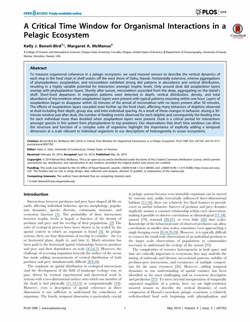
A Critical Time Window for Organismal Interactions in a Pelagic Ecosystem Kelly J. Benoit-Bird 1 *, Margaret A. McManus 2 1 College of Oceanic and Atmospheric Sciences, Oregon State University, Corvallis, Oregon, United States of America, 2 Department of Oceanography, University of Hawaii Manoa, Honolulu, Hawaii, USA Abstract To measure organismal coherence in a pelagic ecosystem, we used moored sensors to describe the vertical dynamics of each step in the food chain in shelf waters off the west shore of Oahu, Hawaii. Horizontally extensive, intense aggregations of phytoplankton, zooplankton, and micronekton exhibited strong diel patterns in abundance and vertical distribution, resulting in a highly variable potential for interaction amongst trophic levels. Only around dusk did zooplankton layers overlap with phytoplankton layers. Shortly after sunset, micronekton ascended from the deep, aggregating on the island’s shelf. Short-lived departures in migration patterns were detected in depth, vertical distribution, density, and total abundance of micronekton when zooplankton layers were present with typical patterns resuming within one hour. Layers of zooplankton began to disappear within 20 minutes of the arrival of micronekton with no layers present after 50 minutes. The effects of zooplankton layers cascaded even further up the food chain, affecting many behaviors of dolphins observed at dusk including their depth, group size, and inter-individual spacing. As a result of these changes in behavior, during a 30- minute window just after dusk, the number of feeding events observed for each dolphin and consequently the feeding time for each individual more than doubled when zooplankton layers were present. Dusk is a critical period for interactions amongst species in this system from phytoplankton to top predators. Our observations that short time windows can drive the structure and function of a complex suite of organisms highlight the importance of explicitly adding a temporal dimension at a scale relevant to individual organisms to our descriptions of heterogeneity in ocean ecosystems. Citation: Benoit-Bird KJ, McManus MA (2014) A Critical Time Window for Organismal Interactions in a Pelagic Ecosystem. PLoS ONE 9(5): e97763. doi:10.1371/ journal.pone.0097763 Editor: Hans G. Dam, University of Connecticut, United States of America Received February 20, 2014; Accepted April 23, 2014; Published May 20, 2014 Copyright: ß 2014 Benoit-Bird, McManus. This is an open-access article distributed under the terms of the Creative Commons Attribution License, which permits unrestricted use, distribution, and reproduction in any medium, provided the original author and source are credited. Funding: This work was funded by the US Office of Naval Research, awards #N00014-08-1-1212 (MAM), and #N00014-08-1-1210 (KJBB); http://www.onr.navy. mil/. The funders had no role in study design, data collection and analysis, decision to publish, or preparation of the manuscript. Competing Interests: The authors have declared that no competing interests exist. * E-mail: [email protected] Introduction Interactions between predators and prey have shaped all life on earth, affecting individual behavior, species morphology, popula- tion dynamics, species diversity, community structure, and ecosystem function [1]. The probability of these interactions between trophic levels is largely a function of the density of predator and prey and the overlap of their populations. [2] The roles of ecological process have been shown to be scaled by the spatial context in which an organism is found [3]. In pelagic systems, there are four dimensions of overlap to consider – the x-y or horizontal plane, depth (z), and time (t). Much attention has been paid to the horizontal spatial relationships between predator and prey and their dependence on scale [4,5,6,7]. However, the challenge of accessing organisms beneath the surface of the ocean has made adding measurements of vertical distribution of both predator and prey simultaneously difficult [8,9,10]. The emphasis on spatial distribution in ecological interactions (and the development of the field of landscape ecology) was, in part, driven by seminal experimental and theoretical work in systems with a two-dimensional surface onto which one member of the dyad is tied physically [11,12,13] or computationally [14]. However, even a description of spatial coherence in three dimensions is not sufficient to understand the coincidence of organisms. The fourth, temporal dimension is particularly crucial in pelagic systems because even immobile organisms can be moved by currents and, unlike terrestrially influenced three-dimensional habitats [15,16], there are relatively few fixed features to provide cover or anchor behavior. Surveys of predator and prey densities implicitly assume a constant relationship within each observation, making it possible to observe correlations at climatological [17,18], annual [19], seasonal [20,21], or even daily [22] time scales. Knowledge of the behavioral state of observed predators can allow correlations at smaller time scales, sometimes even approaching a single foraging event [8,10,23,24]. However, it is typically difficult to connect the small scale observations of an individual predator to the larger scale observations of populations or communities necessary to understand the ecology of the system [25]. The complexities of resource heterogeneity in both space and time are critically important to ecosystems; they may underlie the timing of outbreaks and blooms, successional patterns, stability of predator-prey interactions, and coexistence of multiple competi- tors for the same resources [26]. However, adding temporal dynamics to our understanding of spatial variance has been identified as the most challenging task in ecosystem description and prediction [27]. To move beyond interpretation of temporally separated snapshots of a system, here, we use high-resolution moored sensors to describe the vertical dynamics of each component of Hawaii’s nearshore pelagic ecosystem, a relatively well-described food web beginning with phytoplankton and PLOS ONE | www.plosone.org 1 May 2014 | Volume 9 | Issue 5 | e97763
-
Upload
independent -
Category
Documents
-
view
0 -
download
0
Transcript of A Critical Time Window for Organismal Interactions in a Pelagic Ecosystem
A Critical Time Window for Organismal Interactions in aPelagic EcosystemKelly J. Benoit-Bird1*, Margaret A. McManus2
1 College of Oceanic and Atmospheric Sciences, Oregon State University, Corvallis, Oregon, United States of America, 2 Department of Oceanography, University of Hawaii
Manoa, Honolulu, Hawaii, USA
Abstract
To measure organismal coherence in a pelagic ecosystem, we used moored sensors to describe the vertical dynamics ofeach step in the food chain in shelf waters off the west shore of Oahu, Hawaii. Horizontally extensive, intense aggregationsof phytoplankton, zooplankton, and micronekton exhibited strong diel patterns in abundance and vertical distribution,resulting in a highly variable potential for interaction amongst trophic levels. Only around dusk did zooplankton layersoverlap with phytoplankton layers. Shortly after sunset, micronekton ascended from the deep, aggregating on the island’sshelf. Short-lived departures in migration patterns were detected in depth, vertical distribution, density, and totalabundance of micronekton when zooplankton layers were present with typical patterns resuming within one hour. Layers ofzooplankton began to disappear within 20 minutes of the arrival of micronekton with no layers present after 50 minutes.The effects of zooplankton layers cascaded even further up the food chain, affecting many behaviors of dolphins observedat dusk including their depth, group size, and inter-individual spacing. As a result of these changes in behavior, during a 30-minute window just after dusk, the number of feeding events observed for each dolphin and consequently the feeding timefor each individual more than doubled when zooplankton layers were present. Dusk is a critical period for interactionsamongst species in this system from phytoplankton to top predators. Our observations that short time windows can drivethe structure and function of a complex suite of organisms highlight the importance of explicitly adding a temporaldimension at a scale relevant to individual organisms to our descriptions of heterogeneity in ocean ecosystems.
Citation: Benoit-Bird KJ, McManus MA (2014) A Critical Time Window for Organismal Interactions in a Pelagic Ecosystem. PLoS ONE 9(5): e97763. doi:10.1371/journal.pone.0097763
Editor: Hans G. Dam, University of Connecticut, United States of America
Received February 20, 2014; Accepted April 23, 2014; Published May 20, 2014
Copyright: � 2014 Benoit-Bird, McManus. This is an open-access article distributed under the terms of the Creative Commons Attribution License, which permitsunrestricted use, distribution, and reproduction in any medium, provided the original author and source are credited.
Funding: This work was funded by the US Office of Naval Research, awards #N00014-08-1-1212 (MAM), and #N00014-08-1-1210 (KJBB); http://www.onr.navy.mil/. The funders had no role in study design, data collection and analysis, decision to publish, or preparation of the manuscript.
Competing Interests: The authors have declared that no competing interests exist.
* E-mail: [email protected]
Introduction
Interactions between predators and prey have shaped all life on
earth, affecting individual behavior, species morphology, popula-
tion dynamics, species diversity, community structure, and
ecosystem function [1]. The probability of these interactions
between trophic levels is largely a function of the density of
predator and prey and the overlap of their populations. [2] The
roles of ecological process have been shown to be scaled by the
spatial context in which an organism is found [3]. In pelagic
systems, there are four dimensions of overlap to consider – the x-y
or horizontal plane, depth (z), and time (t). Much attention has
been paid to the horizontal spatial relationships between predator
and prey and their dependence on scale [4,5,6,7]. However, the
challenge of accessing organisms beneath the surface of the ocean
has made adding measurements of vertical distribution of both
predator and prey simultaneously difficult [8,9,10].
The emphasis on spatial distribution in ecological interactions
(and the development of the field of landscape ecology) was, in
part, driven by seminal experimental and theoretical work in
systems with a two-dimensional surface onto which one member of
the dyad is tied physically [11,12,13] or computationally [14].
However, even a description of spatial coherence in three
dimensions is not sufficient to understand the coincidence of
organisms. The fourth, temporal dimension is particularly crucial
in pelagic systems because even immobile organisms can be moved
by currents and, unlike terrestrially influenced three-dimensional
habitats [15,16], there are relatively few fixed features to provide
cover or anchor behavior. Surveys of predator and prey densities
implicitly assume a constant relationship within each observation,
making it possible to observe correlations at climatological [17,18],
annual [19], seasonal [20,21], or even daily [22] time scales.
Knowledge of the behavioral state of observed predators can allow
correlations at smaller time scales, sometimes even approaching a
single foraging event [8,10,23,24]. However, it is typically difficult
to connect the small scale observations of an individual predator to
the larger scale observations of populations or communities
necessary to understand the ecology of the system [25].
The complexities of resource heterogeneity in both space and
time are critically important to ecosystems; they may underlie the
timing of outbreaks and blooms, successional patterns, stability of
predator-prey interactions, and coexistence of multiple competi-
tors for the same resources [26]. However, adding temporal
dynamics to our understanding of spatial variance has been
identified as the most challenging task in ecosystem description
and prediction [27]. To move beyond interpretation of temporally
separated snapshots of a system, here, we use high-resolution
moored sensors to describe the vertical dynamics of each
component of Hawaii’s nearshore pelagic ecosystem, a relatively
well-described food web beginning with phytoplankton and
PLOS ONE | www.plosone.org 1 May 2014 | Volume 9 | Issue 5 | e97763
culminating in spinner dolphins (Stenella longirostris). The distribu-
tion of biomass in each of these trophic levels is spatially
heterogeneous, which we showed in previous analyses affects
predator-prey interactions throughout the system [28]. In
describing the importance of spatial pattern, however, our
previous efforts did not measure true coherence between predators
and prey as they focused on long-term temporal dynamics. By not
addressing vertical position of aggregations of organisms in the
water column or time variance at scales of less than a day, the
mechanisms of these interactions remain obscured. Particularly as
short time scales and vertical position are predicted to be
important based on the strong diel patterns in both local biomass
and vertical distribution observed in each step of the food chain
(spinner dolphins [23]; zooplankton [29]; phytoplankton [30];
micronekton [31]). In this contribution, we use fine vertical (tens of
cms) and temporal (one sample every second to every 15 minutes,
depending on the instrument) resolution descriptions of the
distribution of biomass in the food web to elucidate the
interactions between predators and prey in both space and time.
Methods
Over two, three-week periods in the spring of 2009 and 2010,
we used moored sensors complemented by shipboard surveys to
measure the physical and biological properties of the shelf off the
leeward coast of Oahu, Hawaii. This section of coastline runs
north to south with little variation, and isobaths are roughly
parallel to the shoreline. The study was conducted near the 25 m
isobath from 20 April to 12 May 2009 and 10 April to 5 May 2010
in the area of 21u 30.5 N, 158u 14.2 W (Figure 1), roughly 1 km
from the shoreline and 5 km inshore of the habitat that serves as
the daytime habitat for mesopelagic animals of the deep-scattering
layer [31].
Ethics StatementObservations of spinner dolphins were conducted under a US
National Marine Fisheries Service Permit 1000–1617. The area
accessed was not privately owned or protected and no protected
species were sampled. This effort complied with all relevant
regulations.
MooringsA moored autonomous profiler (the Seahorse; Brooke Ocean
Technology) collected temperature, salinity, pressure (SeaBird
SBE-19 CTD), dissolved oxygen (SBE-43), and chlorophyll
fluorescence (WET Labs ECO-FLS) data every 30 minutes
between the near-bottom and the near-surface with ,1 cm
vertical resolution.
Throughout each study period, an upward looking multi-
frequency echosounder (ASL Environmental Acoustic Water
Column Profiler: 200, 420, 740 kHz) collected acoustic backscat-
ter data from zooplankton, micronekton, and dolphins once per
second. The echosounder used a pulse length of 256 ms, had a 3-
dB beamwidth of 7 degrees, and a vertical resolution of 1 cm. The
echosounder was calibrated in two ways: in a seawater tank using a
reference sphere [32] and at sea using both a reference target as
well as a comparative approach with the calibrated shipboard
echosounders.
Shipboard samplingShip-based sampling was conducted from the 9 m Alyce C.
anchored near the moored sensors. Sampling of zooplankton,
micronekton and dolphins with echosounders and phytoplankton,
zooplankton, and micronekton with a high-resolution profiling
package was carried out continuously for 24 hours during the full,
new, and quarter moon phases in each year. Additional sampling
conducted over eight shorter intervals in each year that were
dispersed over each study period. These efforts were supplemented
by periodic zooplankton net tows and phytoplankton bottle
samples.
EchosoundersDownward-looking echosounders mounted 1 m below the
surface (calibrated [32] split-beam Simrad EK 60 s at 38 kHz
(12u beamwidth) and 70, 120, and 200 kHz (7u beamwidth) and
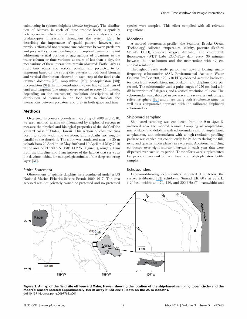
Figure 1. A map of the field site off leeward Oahu, Hawaii showing the location of the ship-based sampling (open circle) and themoored sensors located approximately 100 m away (filled circle), both on the 25 m isobaths.doi:10.1371/journal.pone.0097763.g001
Critical Time Windows for Pelagic Interactions
PLOS ONE | www.plosone.org 2 May 2014 | Volume 9 | Issue 5 | e97763

Simrad ES60, 5u single beam at 710 kHz, each with an outgoing
pulse length of 256 ms and a pulse rate of 8–10 Hz) were used to
continuously measure the distribution and density of micronekton
and zooplankton aggregations. A 200 kHz multibeam sonar
(Kongsberg-Mesotech SM2000) was also deployed on the rigid
pole. This system has a 120 degree by 1 degree field of view that
was used to observe groups of foraging dolphins [23].
ProfilerThe physical and biological characteristics of the water column
were measured near-continuously with a profiling package during
each sampling period. Profiles covered 1 m from the surface to
1 m above the bottom approximately every 4 minutes throughout
each sampling period. To maximize the vertical resolution of the
profiles the instrument package was ballasted to achieve an
average descent rate of 10 cm s21 and was decoupled from ship
motion during descent by allowing cables to remain slack. The
profiling package was equipped with a CTD (SeaBird 25;
temperature, salinity, pressure), a dissolved oxygen sensor (SBE-
43), and a fluorometer to measure chlorophyll a fluorescence
(WETLabs WETStar). Data from CTD casts were low passed
filtered and edited for loops before the raw variables were
converted to variables of interest using factory calibrations.
The profiling package also had a Tracor acoustic profiling
system (TAPS) which uses acoustical scattering at six frequencies
(265, 420, 700, 1100, 1850 and 3000 kHz) to quantitatively
estimate zooplankton abundance in size classes [33]. Volume
scattering strength profiles were averaged into 0.2 m vertical bins
and transformed to estimates of zooplankton biovolume in
equivalent spherical diameter (ESD) classes via a constrained,
non-linear, least-squares algorithm [34,35,36], that employed a
simple spherical model; a choice guided by the body forms
observed in net tows. These estimates of biovolume were
converted to estimates of density by dividing the biovolume at a
given size by the volume of a spherical animal of that ESD. Large
individual targets (e.g. micronekton) were rarely sampled due to
the small sample volume of TAPS (about 3 l). After initial
processing, TAPS profiles were analyzed for the presence of
discrete layers, as well as vertically integrated to provide an
estimate of total zooplankton abundance.
To obtain information on the taxonomic composition, numer-
ical density, and size of micronekton, the profiler was equipped
with a two-camera low-light video system with infrared illumina-
tion. Still views were extracted every 0.25 m from each of the two
cameras and analyzed following Benoit-Bird and Au [31].
Net towsPeriodically throughout shipboard sampling efforts, vertical net
tows were conducted with a 0.5 m opening/closing, 200 mm mesh
net equipped with a pressure sensor with real time communication
(Simrad PI32) and flow meter modified to spin only on the upcast
(General Oceanics). These tows were used to provide information
on the identity and density of zooplankton in identified features
and more generally throughout the water column. When an
acoustic feature of interest was identified during shipboard
sampling, the feature was discretely sampled at least once. Each
targeted samples was followed by a sample integrated from 1 m
above the bottom to the surface. Water-column integrated samples
were also taken at regular intervals when no features of interest
were identified. Samples were preserved in a buffered 5% formalin
solution in seawater for later analysis following the methods
described in Benoit-Bird et al.[29].
Data Analysis
Echosounder dataAll echosounder data were analyzed using Myriax’s Echoview
software. For shipboard echosounders, all echoes from solitary
individual targets, that is targets at densities lower than one per
sampling volume were identified as large individual fish or marine
mammals and removed from the data. In moored data, intense,
large targets that were present at all frequencies were identified as
marine mammals [23] and removed from the data set. The
remaining volume scattering data from both the shipboard and
moored sensors were thresholded at a value of 280 dB and
integrated in 10 second horizontal by 0.30 m vertical bins. The
volume scattering in each bin was then compared across all
frequencies. Those bins that had volume scattering that did not
increase by more than 2 dB with any increasing step in frequency
were classified as micronektonic animals [37]. Of the remaining
bins, those that had the scattering at least 4 dB higher at the two
highest frequencies used than the lowest were classified as
zooplankton [38,39]. These two classifications accounted for
95% of all intervals for both echosounder systems.
Using only data classified as zooplankton, the total scattering at
200 and 710 kHz for the shipboard echosounders and 420 and
740 kHz for the moored echosounder were integrated over the
entire water column in 10 s bins. Using only data classified as
micronekton, raw 200 kHz volume scattering from both the
moored and shipboard echosounders was integrated into 10
second by 0.5 m bins. Numerical density of micronektonic animals
was calculated from the 200 kHz volume scattering data,
determined to be the most accurate frequency for this estimate
[37], using echo energy integration. Estimates of individual target
strength were made by combining laboratory target strength
measurements with animal size and identity information from the
video system on the high-resolution profiler averaged across all
recordings made at the same time of day and depth as the
echosoundings.
Identification of biotic layersBoth fluorescence and acoustic scattering were found in
discrete, persistent features or layers. Layers in all data sets were
identified following the general approach detailed in Benoit-Bird
et al. [40] and summarized here. Layers in scattering consistent
with micronekton were identified in the 200 kHz data from both
moored and shipboard echosounders, while layers in scattering
consistent with zooplankton were analyzed at all frequencies
200 kHz and above. A running, 5 m vertical median was taken for
each profile which was an individual cast of TAPS or the
fluorometer or 10 s averaged classified echosounder data (micro-
nekton or zooplankton, analyzed separately) to define the local
background in acoustic scattering or fluorescence. If the maximum
measurement exceeded this background by 1.25 times for at least
two consecutive casts or 30 s of echosounder data, the feature was
considered a layer. The points at which scattering crossed below
the running median were used to define the upper and lower edges
of the layer. Scattering or fluorescence between these two points
was integrated for each layer. Layer peak depth was defined as the
point at which the layer reached a maximum value while median
depth was the depth at which the integrated value within the layer
was split in half. For plankton layers, thickness was calculated as
the range of values within half the peak intensity of the layer,
sometimes called the full width half maximum (FWHM), for
comparison with previous studies. The average of these charac-
teristics was calculated for each detected layer from the mooring
data for statistical comparisons. The persistence of all zooplankton
Critical Time Windows for Pelagic Interactions
PLOS ONE | www.plosone.org 3 May 2014 | Volume 9 | Issue 5 | e97763
layers less than 5 m in thickness was characterized from the
moored echosounder as the total time a layer was identified with
no gaps in detection greater than 10 seconds. This analysis was not
conducted on the time series of fluorescence data because of its low
temporal resolution of one profile every 15 minutes.
Zooplankton effects on micronekton and dolphinsTo test for potential effects on micronekton occurring before
their arrival at the field site, an ANOVA was used to examine the
effects of zooplankton layer presence on the timing of the arrival of
micronekton at the site. To determine if the vertical distribution of
the mesopelagic layer was affected by the presence of a
zooplankton layer, the median depth, thickness, integrated
abundance, and mean density of the layer of mesopelagic animals
was measured on each night 30 min after sunset as well as 2 hours
after sunset as reported by the US Naval Observatory. A multiple
Analysis of Variance (MANOVA) was used to test for the effects of
zooplankton layer presence on micronekton layer characteristics.
An ANOVA was used to determine the effect of zooplankton
layers on spinner dolphin median depth measured 15–45 min
after sunset. To examine other effects of zooplankton on spinner
dolphin behavior. we examined data from 18 days of shipboard
data that covered at least the 30 minutes before sunset and two
hours after. On 11 of these days a zooplankton layer was present.
Following the methods of Benoit-Bird and Au [23], we used the
multibeam sonar system to count the number of dolphins within
each foraging group, the average spacing between pairs of
dolphins within each foraging group, and the average time each
pair spent inside the circle of foraging dolphins, a measure of
feeding time for all groups observed 15–45 minutes and 90–120
minutes after sunset. We used a MANOVA with sampling date as
a covariate to determine if there was a significant effect of
zooplankton layer presence on these measures of spinner dolphin
behavior in each time interval. We counted the number of dolphin
groups observed during each of these 30 minute intervals and used
an ANOVA to determine if there was an effect of zooplankton
layer presence on the number of dolphin groups observed.
Micronekton effects on zooplankton layersTo examine the impact of micronekton on zooplankton layers,
scattering at 740 kHz from the moored echosounder was
integrated over the thickness of detected zooplankton layers.
Scattering within a layer was tracked in 5 minute intervals from 15
minutes before the first detection of micronektonic animals to 60
minutes after. The average value for each layer in the three, 5
minute intervals immediately before the arrival of micronekton
was subtracted from each subsequent observation of the same
feature to normalize the results.
Results
Fluorescent layersA total of 206 discrete, fluorescent layers were identified from
the moored data set. Of these, all but 5 of these were thinner than
5 m. A comparison of layers detected with the echosounder
mooring and those detected with the profiler showed detection
rates and vertical locations coincided. Fluorescence within these
layers accounted for 18%–94% of the water column integrated
fluorescence while layers covered 1–20% of the water column with
the average thickness layer covering about 10% of the water
column’s depth. The fluorescence from phytoplankton layers was
highly disproportionate to their vertical extent.
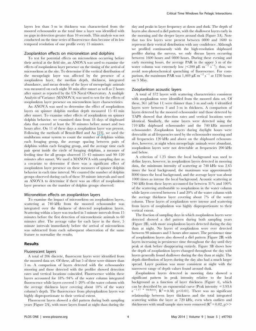
Fluorescent layers showed a diel pattern during both sampling
years (Figure 2A), with more layers found at night than during the
day and peaks in layer frequency at dawn and dusk. The depth of
layers also showed a diel pattern, with the shallowest layers early in
the morning and the deeper layers around dusk (Figure 3A). Note
that too few layers were present between 0800 and 1600 to
represent their vertical distribution with any confidence. Although
we profiled continuously with the high-resolution shipboard
profiler during the surveys, we only discuss layers occurring
between 1600 hours and 0800 hours. During these evening and
early morning hours, the average PAR in the upper 5 m of the
water column was extremely low (,200 mE m22 s21); thus, we
avoid non-photochemical quenching of fluorescence. For com-
parison, the maximum PAR was 1,469 mE m22 s21 at 1230 hours
on 3 May.
Zooplankton acoustic layersA total of 372 layers with scattering characteristics consistent
with zooplankton were identified from the moored data set. Of
these, 361 (all but 11) were thinner than 5 m and only 4 identified
layers were between 3 and 5 m in thickness. A comparison of
layers detected by the moored echosounder and those detected by
TAPS showed that detection rates and vertical locations were
identical. Similarly, the same layers were detected using the
710 kHz shipboard echosounder and the 740 kHz moored
echosounder. Zooplankton layers during daylight hours were
detectable at all frequencies used by the echosounder mooring and
all frequencies 120 kHz and above on the shipboard echosoun-
ders, however, at night when mesopelagic animals were abundant,
zooplankton layers were not detectable at frequencies 200 kHz
and below.
A criterion of 1.25 times the local background was used to
define layers, however, in zooplankton layers detected in mooring
data, the minimum intensity of scattering at 740 kHz was 2.65
times the local background, the maximum was approximately
8000 times the local background, and the average layer was about
1000 times as intense the local background. Acoustic scattering at
740 kHz from these layers accounted for between 31% and 100%
of the scattering attributable to zooplankton in the water column
while layers covered between 1 and 20% of the water column with
the average thickness layer covering about 7% of the water
column. These layers of zooplankton were intense and scattering
from layers of zooplankton was highly disproportionate to their
vertical extent.
The fraction of sampling days in which zooplankton layers were
detected showed a diel pattern during both sampling years
(Figure 2B), with more zooplankton layers detected during the day
than at night. No layers of zooplankton were ever detected
between 90 minutes and 3 hours after sunset. The persistence time
of zooplankton layers also showed a diel pattern (Figure 2B) with
layers increasing in persistence time throughout the day until they
peak at dusk before disappearing entirely. Figure 3B shows how
the depth of zooplankton layers changed throughout the day with
layers generally found shallower during the day than at night. The
depth distribution of layers during the day also had a much larger
spread. Layer position was more consistent at night with the
narrowest range of depth values found around dusk.
Zooplankton layers detected in mooring data showed a
significant pattern in peak intensity relative to the local
background as a function of layer thickness (Figure 4), which
can be described by an exponential curve (Peak intensity = 3.93.6
e21.17 * thickness; R2 = 0.38; p,0.01). There was no significant
relationship between layer thickness and the total integrated
scattering within the layer at 720 kHz, even when outliers and
thicknesses with small sample sizes were removed (R2 = 0.02, p..
Critical Time Windows for Pelagic Interactions
PLOS ONE | www.plosone.org 4 May 2014 | Volume 9 | Issue 5 | e97763
0.05). The median integrated scattering within each layer was
about 250 m2nmi22 at 740 kHz, regardless of layer thickness.
Identification of zooplankton layer constituentsThe frequency response (Sv 740 kHz - Sv 420 kHz) of zooplankton
layers detected by the mooring was bimodal with one mode
centered at 22.5 dB and a larger mode at 5.5 dB (Figure 5).
There were no layers with frequency response values between 2
1.6 and 2.7 dB. Layers with a positive frequency response were
sampled using stratified net tows on 11 occasions. When these
layers were found, net tows, both those that covered the entire
water column and those that targeted acoustic features, were
dominated in both number and biomass by calanoid copepods
between 0.5 and 2.0 mm. The single most abundant group was
Clausocalanus spp. A paired t-test showed that there was a
significant increase in the density of copepods in net tows targeting
the acoustic layers compared to those covering the entire water
column (t = 86.92, df = 10, p..0.05).
The smaller mode in frequency response from the moored
echosounder was accounted for by 31 layers, all detected in the
second half of the 2009 field experiment. On five occasions, layers
with stronger scattering at 420 kHz relative to 740 kHz were
discretely sampled. These net tows were unlike those taken at any
other time during the experiment as they were dominated both in
number and biomass by hyperiid amphipods with equivalent
spherical diameters between 2.6–3.7 mm. Vertically integrated
tows of the entire water column taken at the same time showed no
difference from stratified tows in the total number of amphipods
caught (paired t-test: t = 0.72, df = 4, p..0.05). There was a
significant increase in the total number of copepods in net tows
covering the entire water column relative to the tows targeting just
the layer (paired t-test: t = 11.86, df = 4 p,0.01) but no increase in
copepod density (paired t-test: t = 1.20, df = 4, p..0.05).
Figure 2. The frequency of occurrence of layers of phytoplankton (A) and zooplankton (B) as a function of local time detected usingmoored instruments across the two, 3-week studies is shown in the black symbols and solid lines. The y-axis shows the fraction of the42 sampling days on which layers were detected in each time interval. Dusk and dawn are indicated by dashed lines separating the gray (night) fromwhite (day) regions. Open circles and dashed lines in B indicate the average persistence, the total time a zooplankton layer was identified with nogaps in detection greater than 10 seconds, of zooplankton layers.doi:10.1371/journal.pone.0097763.g002
Critical Time Windows for Pelagic Interactions
PLOS ONE | www.plosone.org 5 May 2014 | Volume 9 | Issue 5 | e97763

Critical Time Windows for Pelagic Interactions
PLOS ONE | www.plosone.org 6 May 2014 | Volume 9 | Issue 5 | e97763

During ship sampling, TAPS profiles were used to characterize
the frequency response of scattering layers, which can provide
information on the type and size of dominant scatterers. The
frequency response of all layers was characteristic of small, fluid-
like scatterers; generally increasing scattering strength with
increasing frequency, sometimes reaching an asymptote at the
highest frequencies with the presence of relatively small local nulls
in scattering [41]. The average scattering responses for the two
types of layers identified from the moored data are shown in
Figure 6.
Overlap of plankton layersThe absolute value of the offset between the peaks of co-
occurring fluorescent and acoustically scattering layers is shown in
Figure 3C. Despite the apparent parallel movements of fluorescent
layers and zooplankton layers, the median offset between paired
layer peaks was less than 2.5 m only between dusk and 0100 h.
Given the average thickness of each layer type (,2.5 m) and the
fact that .90% of the layer’s integrated fluorescence or acoustic
scattering occurred within this thickness, this is the maximum
separation that would allow consistent overlap between individuals
within each layer type. Only at and immediately after dusk was the
offset between layers consistently less than 2.5 m, with layers of
zooplankton consistently deeper than phytoplankton layers
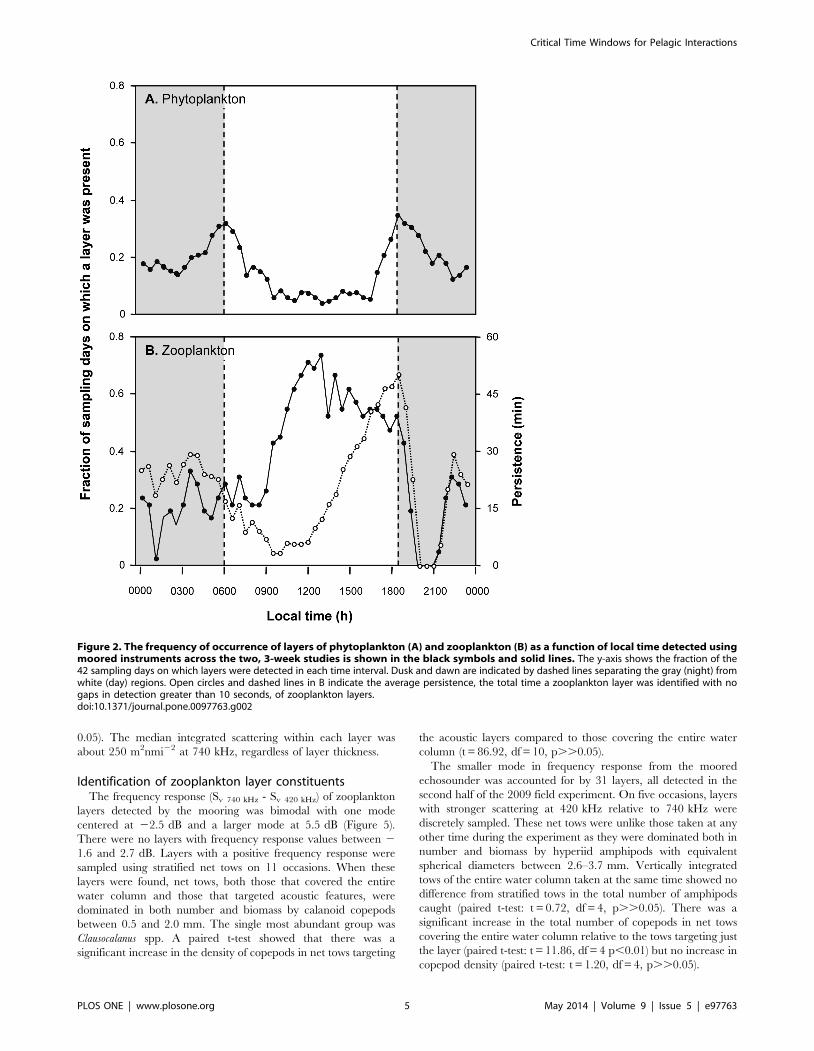
(Figures 7 and 8).
Zooplankton effects on micronekton and spinnerdolphins
The diel migration of micronekton into the shallow waters of
Oahu’s shelf has been well described previously [31,42]. The
general patterns of micronekton during the time periods of this
study matched those observations. For example, previous work has
shown that nearly 100% of the micronekton found at night in
these shallow waters were myctophids [31]. Both the camera
system on the profiler and the frequency response of scattering
from micronekton measured using the shipboard sampling
indicated that held true during this study. However, while timing
of arrival of the micronektonic layer at the 25 m site matched
those observed previously and was not affected by layer presence
(ANOVA: df = 1,25; F = 1.8; p = 0.41), the vertical location of the
layer just after dusk showed more variation relative to previous
studies that measured this time period with coarser temporal
resolution [42]. The vertical distribution of micronekton at dusk
on a night when a mode 2 zooplankton layer was detected is
Figure 3. The peak depth of phytoplankton (A) and zooplankton layers (B) as well as the vertical offset between concurrentlydetected layer peaks (C) is shown as a function of local time. In each plot, heavy bars indicate the median of the distribution, the box oneinterquartile range, and the error bars show the 95% confidence interval.doi:10.1371/journal.pone.0097763.g003
Figure 4. The peak intensity of layers detected at 740 kHz from the moored sensor is shown as a function of layer thickness. Heavybars indicate the median of each distribution, the box one interquartile range, the error bars the 95% confidence interval, open circles outliers, andstars are those values that are least three box lengths from the median. All extreme outliers were mode 1 layers, those that had much strongervolume scattering at 420 than 740 kHz, revealed by net tows to be comprised of hyperrid amphipods rather than the copepods that made up themajority of layers.doi:10.1371/journal.pone.0097763.g004
Critical Time Windows for Pelagic Interactions
PLOS ONE | www.plosone.org 7 May 2014 | Volume 9 | Issue 5 | e97763

shown in Figure 8. The vertical distribution of micronekton at the
same time on the next night when no zooplankton layer was
detected is also shown. A multiple analysis of variance showed that
the presence of zooplankton layers significantly affected the
characteristics of micronekton layers measured just after dusk
(df = 1,25; F = 68.3, p,0.001; Figure 9) but not later in the night
(df = 1,25; F = 0.85, p = 0.91). Between subjects effects tests
showed that there was a significant effect of layer presence on
micronekton median depth (F = 24.3; p,0.005), micronekton
layer thickness (F = 107.6; p,0.001), integrated abundance
(F = 11.5; p,0.01), and micronekton density just after dusk
(F = 46.9; p,0.001). A regression analysis showed a strong, linear
relationship between the peak depth of the zooplankton layer and
the peak depth of the micronekton layer observed on the same
night, both 30 minutes after sunset (micronekton depth = 0.96 *
zooplankton depth – 1.05; r2 = 0.83; p,0.001).
The presence of zooplankton layers had a significant effect on
the mean depth of dolphins observed in the 15–45 minutes after
dusk (Mean dolphin depth: layer present = 19.6 m, ab-
sent = 12.3 m; ANOVA: df = 1,16; F = 17.13; p,0.005) but not
during the 90–120 minutes after dusk (Mean dolphin
depth = 10.28; ANOVA: df = 1,16, F = 1.7; p = 0.51). The pres-
ence of zooplankton layers had a significant effect on the number
of groups of dolphins observed in the 15–45 minutes after dusk
(Average number of groups: layers present = 4.8, absent = 2.6;
ANOVA: F = 30.42; df = 1,16; p,0.001) but again, not during the
later time period (Average number of groups = 3.8; ANOVA:
F = 0.41; p = 0.88). The presence of layers but not sampling date
significantly affected the measured characteristics of dolphin
behavior just after dusk (MANOVA: df = 3,66; Fday = 0.13,
p = 0.94; Flayers = 100.8, p,0.001) but neither was important later
in the night (MANOVA: df = 3,66; Fday = 1.21, p = 0.71;
Flayers = 1.42, p = 0.57). Between subjects effects tests for the time
period just after dusk (df = 1,71) showed that there was a
significant effect of layer presence on foraging dolphin group size
(Mode group size: layers present = 20, absent = 24; F = 20.1; p,
0.001) and average inter-pair spacing within the group (Average
inter-pair spacing: layers present = 3.76 m, absent = 2.77 m;
F = 261.1; p,0.001 for both comparisons) but not on time for a
feeding event by an individual pair (mean = 10.2; F = 0.21,
p = 0.65). Observations that involved the entire feeding stage of
a foraging event (e.g., from the onset of pairs moving into the circle
to surfacing) showed no significant effect of layer presence on the
duration of the feeding stage of foraging events (df = 1,26; F = 1.07,
p = 0.31). As a result, while the duration of each pair of dolphins’
individual feeding event did not increase, the number of feeding
Figure 5. A histogram of the frequency response (Sv 740 kHz - Sv
420 kHz) of layers detected by the moored echosounder. The y-axis shows the fraction of all observations accounted for by each 2 dBfrequency response bin. There were no layers with frequency responsevalues between 21.6 and 2.7 dB.doi:10.1371/journal.pone.0097763.g005
Figure 6. The mean volume scattering for each identified thin layer relative to that measured around 700 kHz (dashed line) isshown as a function of frequency for each of three acoustic instruments. Error bars show standard deviation. A) The frequency response ofmode 1 layers, those that had stronger scattering at 420 kHz relative to 740 kHz in the moored data set. B) The frequency response of mode 2 layers.The gray line in each figure represents the scattering response expected for a fluid sphere of the median size of copepods measured from net tows.doi:10.1371/journal.pone.0097763.g006
Critical Time Windows for Pelagic Interactions
PLOS ONE | www.plosone.org 8 May 2014 | Volume 9 | Issue 5 | e97763

events was affected by the presence of zooplankton layers,
increasing from an average of 2.5 when layers were not present
to 5.1 when layers were present.
Micronekton effects on zooplankton layersTo examine the effect of micronekton on zooplankton layers,
integrated scattering at 740 kHz within a layer was normalized to
the integrated scattering over the 15 minutes before the first
detection of micronekton and tracked in 5-minute intervals from
15 minutes before to 60 minutes after micronekton arrived. The
average value for each layer in the three, 5 minute intervals
immediately before the arrival of micronekton was subtracted
from each subsequent observation of the same feature to
normalize the results. The integrated scattering strength began
to decrease within 15 minutes and layers began to be lost entirely
25 minutes after micronekton arrived at the mooring station
(Figure 10).
Discussion
Our goal in this work was to add temporal dynamics to our
growing understanding of spatial variance in ecosystem processes
in Hawaii’s nearshore pelagic environment. To do this, we used
moored sensors to describe the fine-scale vertical dynamics of each
component of system over a variety of timescales. By measuring
true coherence between predators and prey in both space and
time, we gain insight into the mechanisms underlying the
interactions between these organisms. Considerable attention has
been paid to micronekton aggregations [31,42,43], spinner
dolphins [23], and more recently, phytoplankton aggregations
[30,44] at this site. Our results for these components of the system
are individually consistent with previous descriptions. Micronekton
are present in the nearshore only at night where primarily
myctophid fishes achieve considerable densities. Spinner dolphins
track the migratory patterns of micronekton, foraging primarily in
cooperative groups that herd patches of micronekton into even
more intense aggregations. The overall concentrations of phyto-
plankton in nearshore waters are relatively low, consistent with
other subtropical habitats. However, the regular appearance of
intense (up 5 mg m23), thin (typically less than a few meters) layers
dominated the fluorescence in the water column, accounting for
up to 94% of the water column integrated value.
Zooplankton aggregations in this system have not been well
characterized [29,45] and the critical links involving zooplankton
are only beginning to be explored [28]. During our two, 3-week
study periods, zooplankton layers were relatively common,
occurring during at least some time during every day of the
study. During most of the study, net tows showed that zooplankton
layers were made up of copepods, as was the remainder of the
water column. These dense layers reflected the general compo-
sition of the entire system. However, during the second half of
2009, net tows within layers were dominated by hyperiid
amphipods while in the remainder of the water column, copepods
still dominated by number and biovolume. These differences in
layer composition were reflected in differences in the frequency
response of acoustic backscatter with features made up of
copepods having higher scattering at 740 kHz while features
dominated by hyperiid amphipods showed higher scattering at
420 kHz. The unique zooplankton layers found only in one week
in the second half of the 2009 experiment occurred during a
period of uncommonly persistent low wind speeds and increased
stratification.
Zooplankton within layers dominated the zooplankton biomass
measured in the water column when layers were present. Despite
covering only an average of 10% of the water column’s depth,
zooplankton in layers accounted for between 31 and 100% of the
measured zooplankton biomass. Over the course of our two, 3-
week studies, the average concentrations of copepods in the water
Figure 7. A histogram of the distance between the peaks of simultaneously detected fluorescence and zooplankton layers. The y-axis shows the fraction of all observations accounted for by data within each 0.1 m bin. Positive values indicate the zooplankton layer is shallowerthan the fluorescent feature while negative values mean the zooplankton layer is deeper in the water column than the fluorescent layer.doi:10.1371/journal.pone.0097763.g007
Critical Time Windows for Pelagic Interactions
PLOS ONE | www.plosone.org 9 May 2014 | Volume 9 | Issue 5 | e97763
column were approximately 200 m23 for a biovolume of 400 mm2
m23. The average layer of zooplankton had a density of
zooplankton at its peak of about 5,000 individuals m23 while
the strongest layer had a peak density of over 100,000 individuals
m23. However, these densities covered a very narrow vertical
range, typically less than 3 m so the areal density of a layer was
often lower than its peak density. Despite large differences in the
peak intensity of layers and layer thickness, the integrated
scattering within a layer was relatively constant at 250 m2
nmi22 as thinner layers became more intense but did not contain
more individual zooplankters. The origins of this biomass limit and
its implications are not clear.
Zooplankton layers showed strong, predictable diel patterns in
their occurrence and location in the water column. Zooplankton
layers were most common during the afternoon, disappeared just
after dusk, a pattern also observed in other sites in Hawaii [46],
reappearing just before midnight. Zooplankton layers were found
deep in the water column at night and an average of about 10 m
shallower during the day. Around dusk, the abundant zooplankton
layers showed a very narrow range of depths centered at 20 m,
5 m above the seafloor. This diel pattern is likely to be the result of
behavioral dynamics of the zooplankters, perhaps as a response to
convective overturning that occurs after the sun sets [30].
Layers of fluorescent phytoplankton also showed distinctive diel
patterns with more layers observed at night than during the day
with peaks in layer abundance at dawn and dusk. The peak in
abundance at dusk is consistent with observations by McManus et
al [30], whoalso observed a peak in abundance just before sunset.
This peak is coincident with the time of day when thermal
stratification is the strongest and most persistent [30], however,
that stratification breaks down throughout the night due to
convective overturn and thus cannot explain the somewhat smaller
dawn peak in layer frequency. The depth of fluorescent layers of
phytoplankton was restricted around dusk to just shallower than
20 m. Throughout the night, phytoplankton layers moved
upwards through water column with an increasingly variable
range of depths amongst them until they were within 7 m of the
surface around dawn. During daylight hours, too few phytoplank-
ton layers were identified to characterize their depth distribution.
This limited number of detectable phytoplankton layers during the
Figure 8. A sample profile of fluorescence (thin black line), zooplankton biovolume (gray line), and micronekton density (heavyblack line) measured using shipboard sampling tools 30 minutes after sunset. The zooplankton layer shown was a mode 2 layer comprisedof copepods. The vertical distribution of micronekton at the same time on the next night when no zooplankton layer was detected is shown as adashed black line.doi:10.1371/journal.pone.0097763.g008
Critical Time Windows for Pelagic Interactions
PLOS ONE | www.plosone.org 10 May 2014 | Volume 9 | Issue 5 | e97763
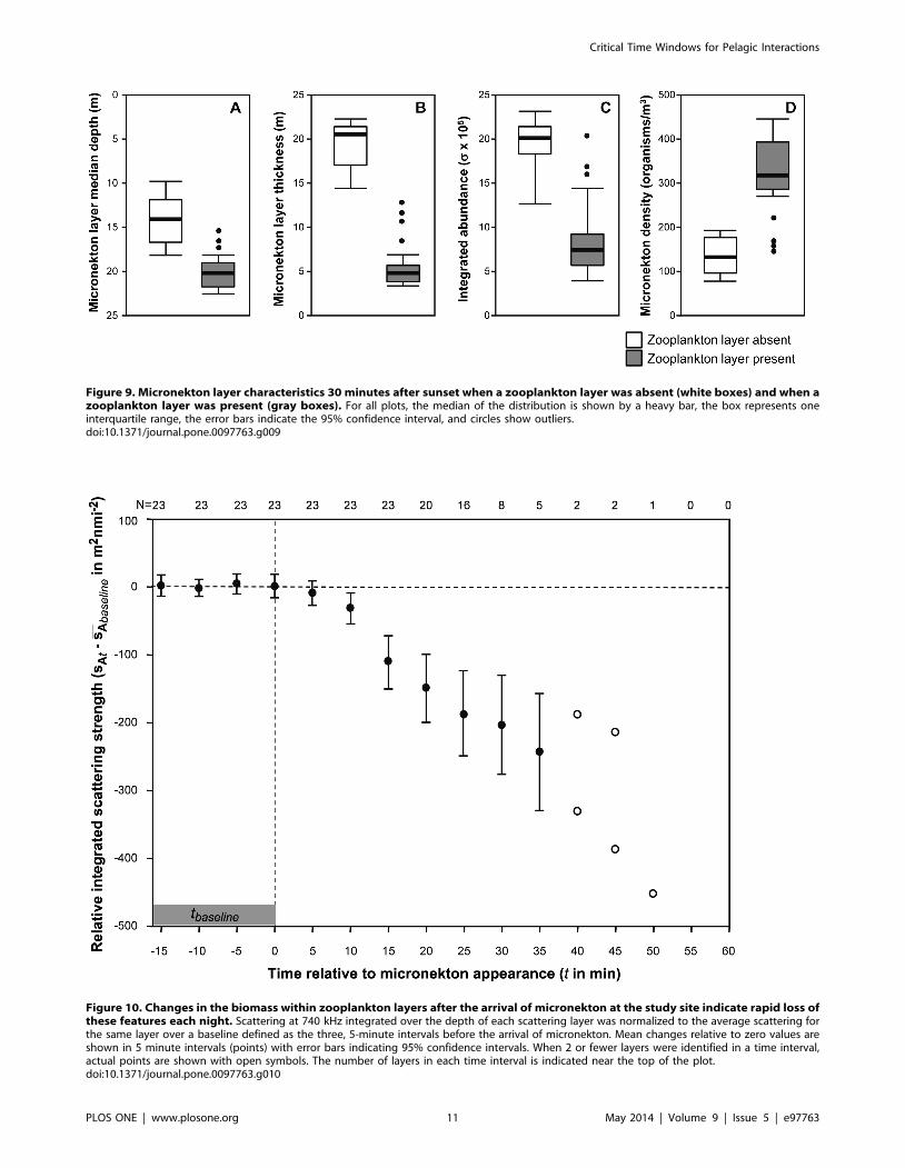
Figure 9. Micronekton layer characteristics 30 minutes after sunset when a zooplankton layer was absent (white boxes) and when azooplankton layer was present (gray boxes). For all plots, the median of the distribution is shown by a heavy bar, the box represents oneinterquartile range, the error bars indicate the 95% confidence interval, and circles show outliers.doi:10.1371/journal.pone.0097763.g009
Figure 10. Changes in the biomass within zooplankton layers after the arrival of micronekton at the study site indicate rapid loss ofthese features each night. Scattering at 740 kHz integrated over the depth of each scattering layer was normalized to the average scattering forthe same layer over a baseline defined as the three, 5-minute intervals before the arrival of micronekton. Mean changes relative to zero values areshown in 5 minute intervals (points) with error bars indicating 95% confidence intervals. When 2 or fewer layers were identified in a time interval,actual points are shown with open symbols. The number of layers in each time interval is indicated near the top of the plot.doi:10.1371/journal.pone.0097763.g010
Critical Time Windows for Pelagic Interactions
PLOS ONE | www.plosone.org 11 May 2014 | Volume 9 | Issue 5 | e97763

day could be due to dispersion of phytoplankton during the day
followed by reformation into layers at dusk, migration of layers to
the surface where they would not be detected by the moored or
shipboard profilers as has been observed in layers of motile
phytoplankton in other habitats [47], or perhaps intense non-
photochemical quenching of fluorescence during the day.
The strong diel patterns of layers of both phytoplankton and
zooplankton result in a highly variable potential for interaction
between the two groups. Layers of phytoplankton and zooplankton
show different temporal trends in their occurrence but similar
patterns in their vertical position in the water column. However,
despite the similar patterns in vertical position, layers that
occurred at the same time did not often occur within a few
meters of each other vertically and the zooplankton layer was
always deeper than the phytoplankton layer so there was no
potential for interaction during vertical crossings of layers. A
significant number of phytoplankton and zooplankton within
layers co-occur in both three-dimensional space and time at night,
however, only just after dusk did the organisms in these layers
predictably overlap. This is consistent with observations of other
copepod species which focus their feeding during dusk and/or
dawn [48]. However, the pattern was quite different from that
observed in Monterey Bay, California where layers of zooplankton
overlapped with phytoplankton infrequently but predictably as a
function of fraction of available phytoplankton in layers and not
diurnal cycling [40]. Interestingly, in the observations here, all
phytoplankton layers contained at least 18% of the total
phytoplankton fluorescence in the water column, the threshold
at which zooplankton layers actively responded to phytoplankton
layers in the richer, temperate waters of Monterey Bay, indicating
different mechanisms for layer co-occurrence.
While not evidence of consumption, overlap between predator
and prey is necessary for foraging and thus only during this less
than one hour each day could zooplankton be consuming
fluorescent phytoplankton found in layers in this system. However,
despite the predictable co-location of layers of phytoplankton and
zooplankton at dusk, complete overlap of these layers did not
occur at this time or any other. The peak of zooplankton layers
was always deeper than the peak of fluorescent layers. At the time
of consistent co-location of layers, throughout all observations the
peak of zooplankton layers was approximately 1 m deeper than
the phytoplankton layer occurring at the same time. As a result,
only the upper ,40% of a layer of zooplankton interacts with the
lower ,30% of the phytoplankton layer. These offsets could be the
result of physical forcing affecting these different sized organisms
differently, a foraging tactic of the predator attacking prey from
beneath, a response of consumers to their own predators, or a
balance of potentially opposing forces. Offsets between layers of
different types of plankton have been observed but only rarely
have small offsets been predictable [40,49,50]. Benoit-Bird et al
[40] found that when fluorescent and acoustic layers were in close
proximity, layer peaks were not coincident but zooplankton were
nearly equally likely to be above the phytoplankton layer as below
it. So, while small offsets between layers of plankton appear to be
common, the factors driving those relationships likely vary
amongst systems and species.
Dusk is also a critical period for other interactions within the
system. Shortly after sunset, micronektonic organisms, primarily
myctophid fishes, ascend from the deep, aggregating on the
narrow island shelf to consume the relatively rich resources present
near the island at night [29,31]. The phenology and typical
vertical distributions of these organisms have been well docu-
mented [42]. We noticed dramatic departures from these typical
patterns whenever dense layers of zooplankton were detected at
dusk as illustrated in Figure 8. The upper edge of micronekton was
not nearly as shallow as expected. This also affected the thickness
of the layer as the bottom edge of the micronekton layer is
constrained by the seafloor, resulting in an increase in the density
of micronekton. The total abundance of micronekton within the
layer, however, decreased as layers reached these high densities.
The effects on micronekton were not observed to be as strong
when zooplankton layers were made up of hyperiid amphipods as
opposed to pelagic copepods. The outliers in Figure 9 were all
measured from zooplankton layers with scattering at 420 kHz that
exceeded that at 740 kHz, associated with large numbers of
hyperiid amphipods in net tows through the layer. These outliers
occurred in a single week during May of 2009, during a period of
uncommonly persistent low wind speeds and increased stratifica-
tion. A preference for copepods is consistent with the known diets
of similar myctophid species in adjacent waters [51].
The presence of a dense, thin layer of zooplankton, particularly
those made up of copepods, caused micronekton to abbreviate
their vertical migration in these shelf waters. This change in
behavior likely allows migrating micronekton to exploit the rich
resource these layers represent. Net tows and acoustic sampling
both reveal that each layer of zooplankton accounted for at least
30% of the total biomass of zooplankton in the water column,
sometimes containing all of the water column’s zooplankton
biomass in the sampling location. It should not be surprising that
zooplankton consumers that move vertically through such layers
either stop moving when they reach the upper limit of these
features or quickly move back into them, particularly if the original
vertical movement was instigated as a quest for food as most
assume nocturnal upward migration to be [52].
The effects of zooplankton layers on micronekton behavior were
relatively short lived. Within an hour of their appearance, all
micronekton were observed to resume their more typical vertical
distribution. Within that same period of time, each zooplankton
layer became undetectable as its integrated acoustic scattering
gradually dropped (Figure 10). Layers of zooplankton began to
disappear within 20 minutes of the arrival of midwater micro-
nekton and all layers were undetectable after 50 minutes. The
disappearance of these layers could be due to dispersion of
individuals or to loss by consumption. After micronekton resumed
their normal movement, layers of zooplankton reappeared
beginning about 2 hours later. The reappearance of layers did
not result in any measurable changes in micronekton despite their
continued co-occurrence in the x-y plane and some vertical
overlap between the lower edge of the micronekton layer and the
zooplankton layer. The reappearance of zooplankton layers would
suggest that dispersion plays some role in the disappearance of
these features after dusk, however dramatically reduced peak
intensities (e.g. 10x or more) indicate that consumption likely plays
a role in their demise as well.
The short temporal overlap between micronekton and zoo-
plankton layers might suggest a limited importance of these
features in the energy acquisition of the micronekton that make a
stop within them. However, simple calculations indicate that
relative increases in foraging gains may indeed by significant. The
density of zooplankton within these layers is at least two orders of
magnitude higher than the average density of all zooplankton in
the water column typical for the same time and location [29]. In
fact, the biomass of zooplankton in the average layer exceeds by
two-fold the average biomass of the entire water column in this
site. If copepods are a preferred food source as indicated by the
increased response to layers made up of copepods relative to those
made up of amphipods, the relative local density difference is even
more striking as zooplankton layers were not representative of the
Critical Time Windows for Pelagic Interactions
PLOS ONE | www.plosone.org 12 May 2014 | Volume 9 | Issue 5 | e97763

entire water column’s zooplankton composition but rather an
intensification only of the copepod community, increasing the
ratio of preferred to non-preferred food resources which may
increase foraging efficiency [53]. Combining estimates of biomass
with Figure 10 shows that after about 30 minutes, the biomass of
zooplankton in layers roughly equals the water column integrated
average. If prey encounter rates for each myctophid are roughly
related to the density of zooplankton in these two conditions, then
those 30 minutes within the layer are equal to approximately
3.5 hours foraging under more typical conditions. If prey
consumption is decreased proportionately with micronekton
density, then the increased density of competitors during that
time could reduce the benefit from a factor of 7 to a factor of ,3, a
likely underestimation of the benefit given results that indicate
higher foraging success rates on more densely aggregated prey
[54,55,56]. However, when foraging time is limited by the day
night cycle to about half of each 24-period, even a factor of 3 for
this short post-dusk time window would result in a ,10% overall
increase in foraging gains.
The presence of layers of zooplankton cascaded even further up
the food, affecting the behavior of dolphins observed at dusk. On
evenings when zooplankton layers were present, spinner dolphins
were an average of 60% deeper in the water column, in groups
that were 17% smaller, with spacing between pairs of dolphins
35% higher and were detected nearly twice as often relative to
those evenings when a zooplankton layer was absent. Perhaps
most importantly, the number of feeding events observed in each
pair of dolphins and consequently the feeding time for each
individual more than doubled when zooplankton layers were
present. These changes only occurred in a 30 minute window just
after dusk, the same time period where significant effects of layer
presence were observed in micronekton. Some of the changes
observed in dolphin behavior may involve costs (deeper diving),
however the increase in the number of feeding events indicate a
net gain as a result of zooplankton layers during the post-dusk time
window. As spinner dolphin foraging is limited by feeding time
rather than directly by the availability of food [23], the doubling in
duration of feeding time over about 5% of their total foraging time
each day could have significant impacts on an individual’s fitness.
Previous analyses of data from the field efforts described here
have shown the importance of the layers of organisms we observed
in their interactions [28]. In part because of the intensity of these
aggregations and strong, once per day patterns, correlations
amongst trophic levels were robust to averaging over each day, a
much longer time scale than the scale at which the interactions
between organism types were occurring. However, this averaging
obscured the details of these interactions. Here, we show that the
interactions driving the overall patterns observed amongst trophic
levels occur over the same very short time interval – within the
hour following sunset each night. The pattern of spatial
coincidence between predator and prey is an emergent outcome
of a behavioral race between them [11,57]. In this case, the
outcome we observed is the result of a number of interdependent
races. The solutions for each step in the trophic level converged at
a short, dynamic period of each day – dusk. Given the changes in
physical processes [30] and the remarkable redistribution of the
animals in the ecosystem [29,42] that occurs at this time, foraging
and avoidance tradeoffs change quickly during this time,
ultimately allowing a brief period of intense interaction between
species. It has long been recognized that dawn and dusk
‘‘transition periods’’ are dynamic and often critical periods for a
variety of species [58,59,60,61] and, as a result, for predator prey
interactions [4]. However, dawn and dusk have often been
explicitly excluded from analyses of diurnal patterns because of the
challenges of obtaining sufficient samples to describe these short
periods.
To understand the interactions between predators and prey in
pelagic systems, we need concurrent data from each that is
coincident and time and space. However, even under ideal
conditions, we must recognize that studies that provide only
snapshots in time are likely to miss the critical periods when
interactions occur amongst species, leaving us with weak or
inconsistent correlations between predator and prey, a common
observation in pelagic ecosystems [5,6,62]. One approach that has
proven helpful in dealing with this challenge for single predator-
prey pairs is to utilize the identification of foraging behavior to
focus sampling efforts [10]. Multi-trophic level interactions,
however, present additional challenges. Because of the importance
of place in Hawaii’s slope associated ecosystem, a fixed network of
sensors that could sample with relatively fine resolution in vertical
space over time allowed us to identify a critical time window for
predator-prey coherence throughout the food chain. Long-term,
multifaceted arrays of ocean sensors are or will soon be coming
online in a variety of pelagic systems. We are optimistic that these
observational tools will provide opportunities to move beyond
examination of temporally separated snapshots towards mecha-
nistic descriptions of ecosystems. Space use decisions by predator
and prey determine the spatial overlap between the two that
affects encounter rates, predation rates and population and
community dynamics [63]. These space use decisions are dynamic
over a variety of time scales, particularly in the constantly moving
fluid environment of the pelagic. While few studies of spatial
ecology have explicitly included a temporal component at scales
smaller than seasonal or larger than single behavioral interactions
or simple day/night contrasts [22], our observations that short
time windows can drive the structure and function of a complex
suite of organisms highlight the importance of explicitly adding a
temporal component to our descriptions of heterogeneity.
Acknowledgments
Chad Waluk, Jeff Sevadjian, Ross Timmerman, Gordon Walker, Linnaea
Jasiuk, Jennifer Patterson, Donn Viviani, Amanda Timmerman, D.
Bloedorm, Lindsey Benjamin, Rebecca Baltes, Gordon Walker, and Jon
Whitney provided assistance in the field. Captains Joe Reich, Tom
Swenarton, and Tony Brown provided logistical support. Tim Cowles,
Mike Chapman of MECCO, and Deep-Sea Power & Light loaned
equipment.
Author Contributions
Conceived and designed the experiments: KJBB MAM. Performed the
experiments: KJBB MAM. Analyzed the data: KJBB MAM. Contributed
reagents/materials/analysis tools: KJBB MAM. Wrote the paper: KJBB
MAM.
References
1. Lima SL (1998) Nonlethal effects in the ecology of predator-prey interactions.
BioScience 48: 25–34.
2. Williamson CE, Stoeckel ME, Schoeneck LJ (1989) Predation risk and the
structure of freshwater zooplankton communities. Oecologia 79: 76–82.
3. Silvertown J, Holtier S, Johnson J, Dale P (1992) Cellular automaton models of
interspecific competition for space—the effect of pattern on process. Journal of
Ecology: 527–533.
4. Rose GA, Leggett WC (1990) The importance of scale to predator-prey spatial
correlations: An example of Atlantic fishes. Ecol 71: 33–43.
Critical Time Windows for Pelagic Interactions
PLOS ONE | www.plosone.org 13 May 2014 | Volume 9 | Issue 5 | e97763

5. Fauchald P (2009) Spatial interaction between seabirds and prey: review and
synthesis. Mar Ecol Prog Ser 391: 139–151.6. Russell RW, Hunt GL, Coyle KO, Cooney RT (1992) Foraging in a fractal
environment: Spatial patterns in a marine predator-prey system. Landscape
Ecology 7: 195–209.7. Hunt G (1990) The pelagic distribution of marine birds in a heterogeneous
environment. Polar Research 8: 43–54.8. Benoit-Bird KJ, Kuletz K, Heppell S, Jones N, Hoover B (2011) Active acoustic
examination of the diving behavior of murres foraging on patchy prey. Mar Ecol
Prog Ser 443: 217–235.9. Williamson CE, Stoeckel ME (1990) Estimating predation risk in zooplankton
communities: the importance of vertical overlap. Hydrobiologia 198: 125–131.10. Hazen EL, Friedlaender AS, Thompson MA, Ware CR, Weinrich MT, et al.
(2009) Fine-scale prey aggregations and foraging ecology of humpback whalesMegaptera novaeangliae. Mar Ecol Prog Ser 395: 75–89.
11. Sih A (1984) The behavioral response race between predator and prey. Am Nat
123: 143–150.12. Bell AV, Rader RB, Peck SL, Sih A (2009) The positive effects of negative
interactions: Can avoidance of competitors or predators increase resourcesampling by prey? Theoretical Population Biology 76: 52–58.
13. Roughgarden J (1974) Population dynamics in a spatially varying environment:
how population size‘‘ tracks’’ spatial variation in carrying capacity. Am Nat:649–664.
14. Lima SL (2002) Putting predators back into behavioral predator-preyinteractions. Trends Ecol Evol 17: 70–75.
15. Nachman G (1981) Temporal and spatial dynamics of an acarine predator-preysystem. The Journal of Animal Ecology: 435–451.
16. Dupuch A, Dill LM, Magnan P (2009) Testing the effects of resource distribution
and inherent habitat riskiness on simultaneous habitat selection by predators andprey. Anim Behav 78: 705–713.
17. Hunt GL, Stabeno PJ, Strom S, Napp JM (2008) Patterns of spatial andtemporal variation in the marine ecosystem of the southeastern Bering Sea, with
special reference to the Pribilof Domain. Deep Sea Research Part II: Topical
Studies in Oceanography 55: 1919–1944.18. Durant JlM, Hjermann DO, Ottersen G, Stenseth NC (2007) Climate and the
match or mismatch between predator requirements and resource availability.Climate Research 33: 271.
19. Sigler MF, Kuletz KJ, Ressler PH, Friday NA, Wilson CD, et al. (2012) Marinepredators and persistent prey in the southeast Bering Sea. Deep Sea Research
Part II: Topical Studies in Oceanography 65–70: 292–303.
20. Womble JN, Sigler MF (2006) Seasonal availability of abundant, energy-richprey influences the abundance and diet of a marine predator, the Steller sea lion
Eumetopias jubatus. Mar Ecol Prog Ser 325: 281–293.21. Simila T, Holst JC, Christensen I (1996) Occurrence and diet of killer whales in
northern Norway: seasonal patterns relative to the distribution and abundance of
Norwegian spring-spawning herring. Can J Fish Aquatic Sci 53: 769–779.22. Hampton SE (2004) Habitat overlap of enemies: temporal patterns and the role
of spatial complexity. Oecologia 138: 475–484.23. Benoit-Bird KJ, Au WWL (2009) Cooperative prey herding by the pelagic
dolphin, Stenella longirostris. J Acoust Soc Am 125: 125–137.24. Sims DW, Witt MJ, Richardson AJ, Southall EJ, Metcalfe JD (2006) Encounter
success of free-ranging marine predator movements across a dynamic prey
landscape. Proceedings of the Royal Society B: Biological Sciences 273: 1195–1201.
25. Schneider DC (2001) The Rise of the Concept of Scale in Ecology: The conceptof scale is evolving from verbal expression to quantitative expression. BioScience
51: 545–553.
26. Grunbaum D (2002) Predicting availability to consumers of spatially andtemporally variable resources. Hydrobiologia 480: 175–191.
27. Horne JK, Schneider DC (1995) Spatial variance in ecology. Oikos 74: 18–26.28. Benoit-Bird KJ, McManus MA (2012) Bottom-up regulation of a pelagic
community through spatial aggregations. Biology Letters 8: 813–816.
29. Benoit-Bird KJ, Zirbel MJ, McManus MA (2008) Diel variation of zooplanktondistributions in Hawaiian waters favors horizontal diel migration by midwater
micronekton. Mar Ecol Prog Ser 367: 109–123.30. McManus MA, Sevadjian JC, Benoit-Bird KJ, Cheriton OM, Timmerman AH,
et al. (2012) Observations of Thin Layers in Coastal Hawaiian Waters. EstuariesCoasts: 1–9.
31. Benoit-Bird KJ, Au WWL (2006) Extreme diel horizontal migrations by a
tropical nearshore resident micronekton community. Mar Ecol Prog Ser 319: 1–14.
32. Foote KG, Vestnes G, Maclennan DN, Simmonds EJ (1987) Calibration ofacoustic instruments for fish density estimation: A practical guide. ICES Coop
Res Rep 144: 57 pages.
33. Holliday DV, Pieper RE (1995) Bioacoustical oceanography at high frequencies.ICES J Mar Sci 52: 279–296.
34. Holliday DV (1977) Extracting biophysical information from the acoustic signals
of marine organisms. In: Anderson NR, Zahuranec BJ, editors. Oceanic SoundScattering Prediction. New York: Plenum. pp. 619–624.
35. Medwin H, Clay C (1997) Fundamentals of Acoustical Oceanography. San
Diego: Academic Press.36. MacLennan DN, Simmonds EJ (1992) Fisheries Acoustics. New York: Chapman
and Hall.37. Benoit-Bird KJ (2009) Effects of scattering layer composition, animal size, and
numerical density on the frequency response of volume backscatter. ICES J Mar
Sci 66: 582–593.38. Korneliussen RJ (2000) Measurement and removal of echo integration noise.
ICES J Mar Sci 57: 1204–1217.39. Kang M, Furusawa M, Miyashita K (2002) Effective and accurate use of
difference in mean volume backscattering strength to identify fish and plankton.ICES J Mar Sci 59: 794–804.
40. Benoit-Bird KJ, Moline MA, Waluk CM, Robbins IC (2010) Integrated
measurements of acoustical and optical thin layers I: Vertical scales ofassociation. Cont Shelf Res 30: 17–28.
41. Stanton TK, Chu D, Wiebe PH (1998) Sound scattering by several zooplanktongroups: II. Scattering models. J Acoust Soc Am 103: 236–253.
42. Benoit-Bird KJ, Au WWL (2004) Diel migration dynamics of an island-
associated sound-scattering layer. Deep-Sea Res 51: 707–719.43. Benoit-Bird KJ, Au WWL (2003) Echo strength and density structure of
Hawaiian mesopelagic boundary community patches. J Acoust Soc Am 114:1888–1897.
44. Sevadjian J, McManus M, Benoit-Bird K, Selph K (2012) Shoreward advectionof phytoplankton and vertical re-distribution of zooplankton by episodic near-
bottom water pulses on an insular shelf: Oahu, Hawaii. Cont Shelf Res.
45. Benoit-Bird KJ, Shroyer EL, McManus MA (2013) A critical scale in planktonaggregations across coastal ecosystems. Geophysical Research Letters in press.
46. Sevadjian J, McManus M, Pawlak G (2010) Effects of physical structure andprocesses on thin zooplankton layers in Mamala Bay, Hawai’i. Mar Ecol Prog
Ser 409: 95–106.
47. Sullivan J, Donaghay P, Rines J (2010) Coastal thin layer dynamics:Consequences to biology and optics. Cont Shelf Res 30: 50–65.
48. Mackas D, Bohrer R (1976) Fluorescence analysis of zooplankton gut contentsand an investigation of diel feeding patterns. J Exp Mar Biol Ecol 25: 77–85.
49. Alldredge AL, Cowles TJ, MacIntyre S, Rines JEB, others a (2002) Occurrenceand mechanism of formation of a dramatic thin layer of marine snow in a
shallow Pacific fjord. Mar Ecol Prog Ser 233.
50. Sevadjian J, McManus M, Ryan J, Greer A, Cowen R, et al. (2014) Across-shorevariability in plankton layering and abundance associated with physical forcing
in Monterey Bay, California. Cont Shelf Res 72: 138–151.51. Clarke TA (1980) Diets of fourteen species of vertically migrating mesopelagic
fishes in Hawaiian waters. Fish Bull 78: 619–640.
52. Enright JT (1977) Diurnal vertical migration: Adaptive significance and timing.Limnol Oceanogr 22: 856–886.
53. Krebs JR (1978) Optimal foraging: Decision rules for predators. In: Krebs JR,Davies NB, editors. Behavioural Ecology, an Evolutionary Approach. Sunder-
land, MA: Sinauer. pp. 23–63.54. Beyer JE (1995) Functional heterogeneity: Using the interrupted poisson process
(IPP) model unit in addressing how food aggregation may affect fish ration. ICES
Council Meeting Papers: 14.55. Lasker R (1975) Field criteria for the survival of anchovy larvae: The relation
between inshore chlorophyll maximum layers and successful first feeding. FishBull 73: 453–462.
56. Leising AW (2001) Copepod foraging in patchy habitats and thin layers using a
2-D individual-based model. Mar Ecol Prog Ser 216: 167–179.57. Abrahams M, Townsend L (1993) Bioluminescence in dinoflagellates: A test of
the burglar alarm hypothesis. Ecol 74: 258–260.58. Ringelberg J (1995) Changes in light intensity and diel vertical migration: A
comparison of marine and freshwater environments. J Mar Biol Assoc UK 75:
15–25.59. Forward R (1988) Diel vertical migration: Zooplankton photobiology and
behavior. Oceanog Mar Biol Annu Rev 26: 361–392.60. Lobel P (1978) Diel, Lunar, and Seasonal Periodicity in the Reproductive
Behavior of the Pomacanthid Fish, Centropyge potteri, and Some Other ReefFishes in Hawaii. Pac Sci 32: 193–207.
61. Freon P, Gerlotto F, Soria M (1996) Diel variability of school structure with
special reference to transition periods. ICES J Mar Sci 53: 459–464.62. Goss C, Bone DG, Peck JM, Everson I, Murray GLJ, et al. (1997) Small-scale
interactions between prions Pachyptila spp. and their zooplankton prey at aninshore site near Bird Island, South Georgia. Mar Ecol Prog Ser 154: 41–51.
63. Sih A (2005) Predator-prey space use as an emergent outcome of a behavioral
response race. Ecology of predator-prey interactions. New York: Oxford. pp.256–278.
Critical Time Windows for Pelagic Interactions
PLOS ONE | www.plosone.org 14 May 2014 | Volume 9 | Issue 5 | e97763