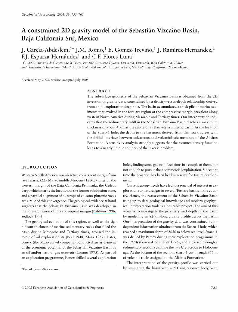
Geophysical Prospecting, 2005, 53, 755–765

A constrained 2D gravity model of the Sebastian Vizcaıno Basin,Baja California Sur, Mexico

J. Garcıa-Abdeslem,1∗ J.M. Romo,1 E. Gomez-Trevino,1 J. Ramırez-Hernandez,2

F.J. Esparza-Hernandez1 and C.F. Flores-Luna1

1CICESE, Division de Ciencias de la Tierra, km 107 Carretera Tijuana–Ensenada, Ensenada, Baja California, 22860,and 2Instituto de Ingenierıa, UABC, Av. de la Normal s/n col. Insurgentes Este, Mexicali, Baja California, 21280 Mexico

Received May 2003, revision accepted July 2005

ABSTRACTThe subsurface geometry of the Sebastian Vizcaıno Basin is obtained from the 2Dinversion of gravity data, constrained by a density-versus-depth relationship derivedfrom an oil exploration deep hole. The basin accumulated a thick pile of marine sed-iments that evolved in the fore-arc region of the compressive margin prevalent alongwestern North America during Mesozoic and Tertiary times. Our interpretation indi-cates that the sedimentary infill in the Sebastian Vizcaıno Basin reaches a maximumthickness of about 4 km at the centre of a relatively symmetric basin. At the locationof the Suaro-1 hole, the depth to the basement derived from this work agrees withthe drilled interface between calcareous and volcaniclastic members of the AlisitosFormation. A sensitivity analysis strongly suggests that the assumed density functionleads to a nearly unique solution of the inverse problem.

I N T R O D U C T I O N

Western North America was an active convergent margin fromlate Triassic (225 Ma) to middle Miocene (12 Ma) times. In thewestern margin of the Baja California Peninsula, the Cedrosdeep, which marks the location of the former subduction zone,and a parallel alignment of outcrops of volcano-plutonic rocksare a relic of this convergence. The geological evidence at handsuggests that the Sebastian Vizcaıno Basin was developed inthe fore-arc region of this convergent margin (Baldwin 1996;Sedlock 1996).

The geological evolution of this region, as well as the sig-nificant thickness of marine sedimentary rocks that filled thebasin during Mesozoic and Tertiary times, aroused the in-terest of oil explorationists (Beal 1948; Mina 1957). Later,Pemex (the Mexican oil company) conducted an assessmentof the economic potential of the Sebastian Vizcaıno Basin asan oil and/or natural-gas reservoir (Lozano 1975). As part ofan exploration programme, Pemex drilled several exploration

∗E-mail: jgarcia@cicese.mx

holes, finding some gas manifestations in a couple of them, butnot enough to pursue their commercial exploitation. Since thattime the prospect has been held in reserve for future develop-ment.

Current energy needs have led to a renewal of interest in ex-ploration for natural gas in several Tertiary basins in the coun-try. Hence, the reassessment of the Sebastian Vizcaıno Basinusing up-to-date geological knowledge and modern geophys-ical interpretation tools is a desirable project. The aim of thiswork is to investigate the geometry and depth of the basinby modelling an 82-km-long gravity profile across the basin.Our interpretation of the gravity data was constrained by in-dependent information obtained from the Suaro-1 hole, whichreached a maximum depth of 2636 m below sea-level. Suaro-1was drilled by Pemex during their exploration programme inthe 1970s (Garcıa-Domınguez 1976), and it passed through asedimentary section spanning the late Cretaceous to Holoceneage. At the bottom of the section, Suaro-1 cut through 355 mof volcanic rocks assigned to the Alisitos Formation.

The interpretation of the gravity profile was carried outby simulating the basin with a 2D single-source body, with

C© 2005 European Association of Geoscientists & Engineers 755

756 J. Garcıa-Abdeslem et al.

113º1 1

28º

115º

0 50 km

114º

25

Sebastián Vizcaíno basin

Vizcaíno Peninsula

Punta EugeniaGuerreroNegro

El Arco

Suaro-1

San Francisquito

Pacific Ocean

Gulf of C

alifornia

Sebas

tián Vizc

aíno Bay

Plio-Quaternary sedimentary rocks: Alluvial, lacustrine andshallow marine deposits.

Plio-Quaternary volcanic rocks: Basalt, andesite and basalticandesite.

Late-Tertiary sedimentary rocks: Marine and continentaldeposits.

Late-Tertiary volcanic rocks: Andesite and basalt from severalvolcanic fields, as well as lava and pyroclastic flows.

Late-Cretaceous sedimentary rocks: Marine deposits.

Cretaceous granitic rocks: Gabbros, diorite, tonalite and granite.

Mesozoic and Palaeozoic metamorphic rocks: Franciscan typecomplex as well as Palaeozoic metasediments.

Jurassic volcanic rocks: Undifferentiated andesite and tuffs, aswell as basalts and gabbros.

Jurassic ophiolitic complex: Serpentinites.

Late-Jurassic sedimentary rocks: Sandstones.

USA

MEXICO

Figure 1 Geological map of the study area. The solid star denotes the location of the Suaro-1 hole.

density contrast varying as a function of depth. The sourcebody is limited on top by the surface topography, and overliesa basement with no density contrast at the bottom. The shapeof the interface between the sedimentary rocks filling the basinand the surrounding basement rocks is defined using a Fourierseries, whose coefficients are found by an inversion algorithmbased on the Marquardt–Levenberg method (Levenberg 1944;Marquardt 1970).

G E O L O G I C A L S E T T I N G

A geological map of the study area is shown in Fig. 1. Thewestern side of the Vizcaıno Peninsula contains a suite of

Triassic to Cretaceous rocks typical of the oceanic crust, de-fined by Sedlock, Ortega-Ramırez and Speed (1993) as theCochimı terrane. According to these authors, this terranewas accreted to western North America about 140 Ma ago,in early Cretaceous times. The compressive margin built bythe Cochimı terrane can be interpreted as an upper plateconsisting of Triassic–Jurassic ophiolitic rocks overriding alower plate consisting of a subduction complex, deformed andmetamorphosed to blueschist facies conditions around 115–104 Ma ago. Both plates are structurally separated by anintervening serpentinite-matrix melange containing a varietyof mafic and ultramafic rocks, as well as exotic blocks ofblueschists, eclogite and amphibolite. It has been postulated

C© 2005 European Association of Geoscientists & Engineers, Geophysical Prospecting, 53, 755–765

A 2D gravity model of the Vizcaıno Basin 757

that extensional deformation of Mesozoic rocks and blueschistexhumation occurred during syn-subduction extension of theNorth American fore-arc between 95 Ma and 20–30 Ma(Baldwin 1996; Sedlock 1996). Unconformably overlying theupper-plate rocks, there is a siliciclastic turbidite sequence ofCretaceous age, and a Miocene–Pliocene siltstone sequencethat discordantly overlies the upper-plate Mesozoic rocks.

Towards the east of the Sebastian Vizcaıno Basin, there isa suite of volcano-plutonic rocks, indicating that igneous ac-tivity was induced by the subduction of oceanic lithosphereinto the underlying mantle. This region, defined by Sedlocket al. (1993) as the Yuma terrane, includes Palaeozoic–Mesozoic metamorphic rocks, as well as Cretaceous rockstypical of a volcanic arc. The Yuma terrane was intruded bygranitoids in the late Cretaceous (∼100 Ma). These granitoidsare exposed from the eastern portion of the study area to theGulf of California. However, south of latitude 28◦N, thesegranitoids are covered by Tertiary and Plio-Quaternary sed-imentary strata and volcanic rocks of andesitic and basalticcomposition.

The stratigraphic column shown in Fig. 2 summarizes thesubsurface geological information provided by the Suaro-1hole. From top to bottom, it shows a 60-m-thick sequenceof Holocene–Pleistocene sediments, consisting chiefly of un-consolidated sand and soil. This Quaternary unit uncon-formably overlies an 1194-m-thick sedimentary sequence ofTertiary age, belonging to the Bateque Formation (Mina 1957)and composed of fine-grained clastics, which were proba-

Figure 2 Stratigraphic column at the Suaro-1 hole.

bly deposited in neritic conditions (Garcıa-Domınguez 1976;Helenes 1984). An early Palaeocene to middle Eocene age hasbeen assigned to these rocks, based on planktonic foraminiferaand dinoflagellate assemblages (Helenes 1984). Underlyingthe Bateque Formation is a 967-m-thick sedimentary se-quence of upper Cretaceous rocks composed of interbed-ded shales, sandstones and some conglomerates (Garcıa-Domınguez 1976), belonging to the Valle Formation (Mina1957). Foraminifera and dinoflagellates found in these strataindicate that, in general, they encompass the Cenomanian toMaastrichtian interval (Helenes 1984). Conformably underly-ing the Valle Formation are lower Cretaceous (Albian–Aptian)rocks belonging to the Alisitos Formation (Allison 1974). Thislast unit is composed of a 90-m-thick biohermal intraclasticlimestone, underlain by a 265-m-thick sequence composed oftuffs and tuffaceous siltstones and breccias where the Suaro-1 reached its total depth (Garcıa-Domınguez 1976; Helenes1984).

T H E G R AV I T Y D ATA

During the spring of 2000 a gravity survey was conductedon the Sebastian Vizcaıno Basin, in which the vertical com-ponent of the gravity field was measured at 150 sites. Theelevation at the gravity stations was determined with an un-certainty of ± 0.25 m, by using two GPS receivers operatingin differential mode. The observed gravity was converted toabsolute gravity by tying these data to an absolute gravitynetwork deployed by INEGI (1990) along the Baja CaliforniaPeninsula. The gravity anomaly was computed by subtractingthe theoretical gravity, computed with the 1997 InternationalGravity Formula (Blakely 1995), from the observed gravity,and the free-air gravity anomaly was computed using a ver-tical gravity gradient of 0.3086 mGal/m. The free-air gravitydata collected in the study were combined with a regional free-air gravity data set compiled by INEGI (1990).

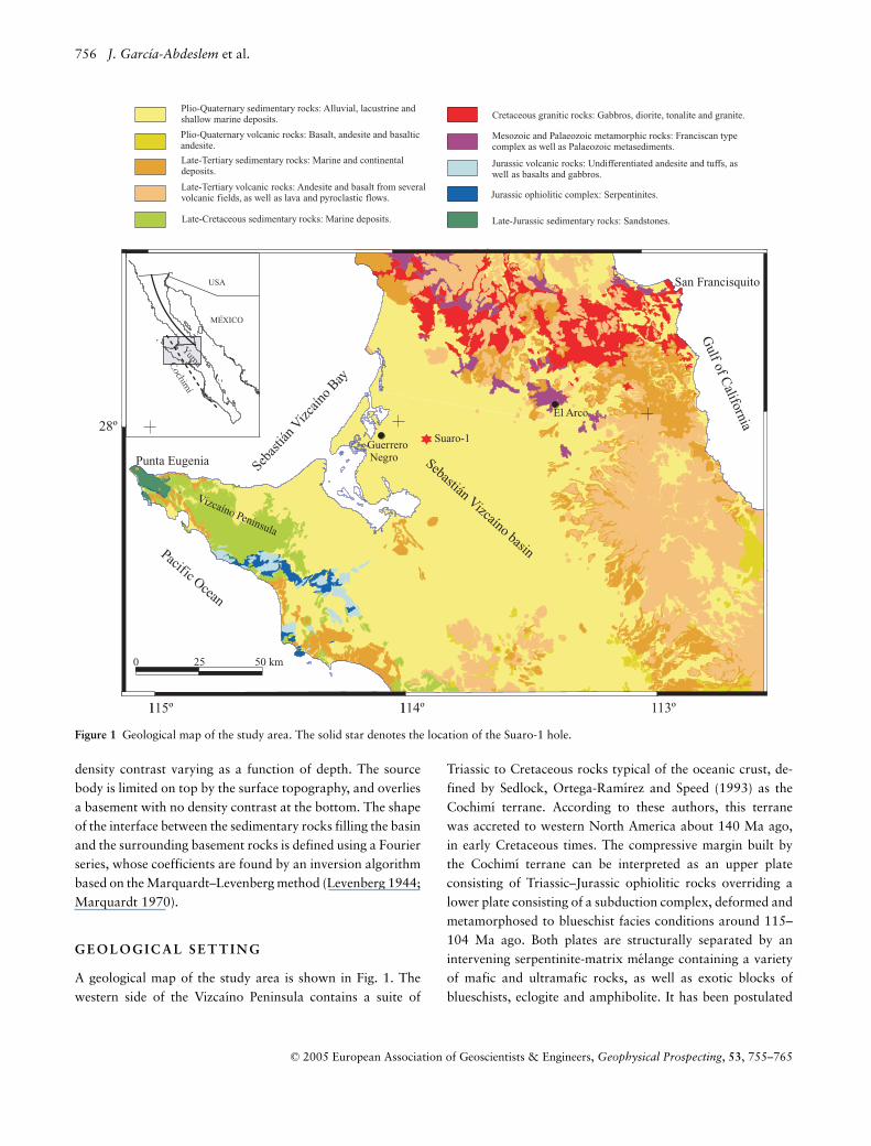
The complete Bouguer anomaly was computed by a methoddescribed by Garcıa-Abdeslem and Martın-Atienza (2001), us-ing a digital elevation model that covers a region of about2 × 2 degrees, with nodes every 100 m (INEGI 1995) and thestandard Bouguer density of 2.67 g/cm3. The Bouguer den-sity was taken as the average value for the different kinds ofrocks outcropping (Fig. 1) in the region considered for thiscomputation.

The complete Bouguer anomaly map (Fig. 3) shows a largeminimum (down to −52 mGal) over the basin and extend-ing offshore into Sebastian Vizcaıno Bay. The gravity mini-mum extends towards the southeast, but it is interrupted by a

C© 2005 European Association of Geoscientists & Engineers, Geophysical Prospecting, 53, 755–765

758 J. Garcıa-Abdeslem et al.

Figure 3 Topographic image map showing the complete Bouguer anomaly with contours every 10 mGal, computed using a density of2.67 g/cm3. The line +—+ shows the location of the interpreted gravity profile, and the solid star denotes the location of the Suaro-1 hole.

narrow gravity high that reaches some 20 mGal, suggesting abasement uplift that divides the basin in two parts.

T H E C O N S T R A I N T

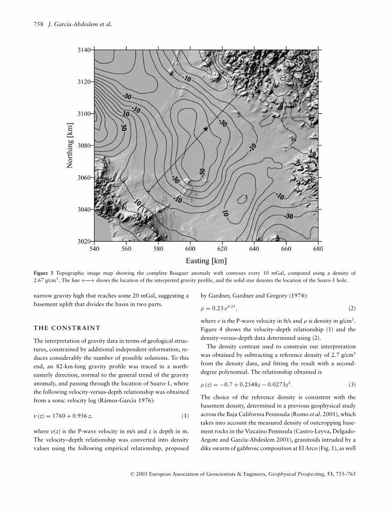
The interpretation of gravity data in terms of geological struc-tures, constrained by additional independent information, re-duces considerably the number of possible solutions. To thisend, an 82-km-long gravity profile was traced in a north-easterly direction, normal to the general trend of the gravityanomaly, and passing through the location of Suaro-1, wherethe following velocity-versus-depth relationship was obtainedfrom a sonic velocity log (Ramos-Garcıa 1976):

v (z) = 1760 + 0.956 z, (1)

where v(z) is the P-wave velocity in m/s and z is depth in m.The velocity–depth relationship was converted into densityvalues using the following empirical relationship, proposed

by Gardner, Gardner and Gregory (1974):

ρ = 0.23 v0.25, (2)

where v is the P-wave velocity in ft/s and ρ is density in g/cm3.Figure 4 shows the velocity–depth relationship (1) and thedensity-versus-depth data determined using (2).

The density contrast used to constrain our interpretationwas obtained by subtracting a reference density of 2.7 g/cm3

from the density data, and fitting the result with a second-degree polynomial. The relationship obtained is

ρ (z) = −0.7 + 0.2548z − 0.0273z2. (3)

The choice of the reference density is consistent with thebasement density, determined in a previous geophysical studyacross the Baja California Peninsula (Romo et al. 2001), whichtakes into account the measured density of outcropping base-ment rocks in the Vizcaıno Peninsula (Castro-Leyva, Delgado-Argote and Garcıa-Abdeslem 2001), granitoids intruded by adike swarm of gabbroic composition at El Arco (Fig. 1), as well

C© 2005 European Association of Geoscientists & Engineers, Geophysical Prospecting, 53, 755–765

A 2D gravity model of the Vizcaıno Basin 759

(a)

1.0

1.5

2.0

2.5

3.0

3.5

4.0

0.0 0.5 1.0 1.5 2.0

Vel

ocit

y[k

m/s

]

(b)

1.8

2.0

2.2

2.4

2.6

0.0 0.5 1.0 1.5 2.0

Depth [km]

Den

sity

[g/

cm3 ]

Figure 4 (a) Linear-velocity versus depth obtained from a sonic log inthe Suaro-1 hole. (b) Density versus depth computed using the empir-ical relationship of Gardner et al. (1974).

as the widespread volcanic rocks of andesitic and basaltic com-position belonging to the volcanic arc. It should be mentionedthat the density-versus-depth relationship is strictly valid onlyat the depth interval drilled in the Suaro-1 hole, as it was ob-tained from the sonic velocity log, but it has been assumed tobe valid at depths greater than 2 km.

T H E F O RWA R D G R AV I T Y P R O B L E M

The vertical component of the gravity field at any exteriorpoint of a 2D source body with density contrast varying withdepth (Garcıa-Abdeslem 2003) is given by

g (x0, y0) = 2γ

∫ X2

X1

dx∫ h2(x)

h1(x)dz

ρ (z) ZX2 + Z2

, (4)

where γ is Newton’s gravitational constant, (x,z) are the co-ordinates of a material point within the source body, (x0,z0)are the observation coordinates, and X = x − x0 and Z = z −z0. The limits of the source body are X1 ≤ x ≤ X2, where x isthe horizontal distance, and z is the depth, defined as positivedownwards. The topography and the interface between thesource body and the basement are represented, respectively,by the functions h1(x) and h2(x), and the density contrast is

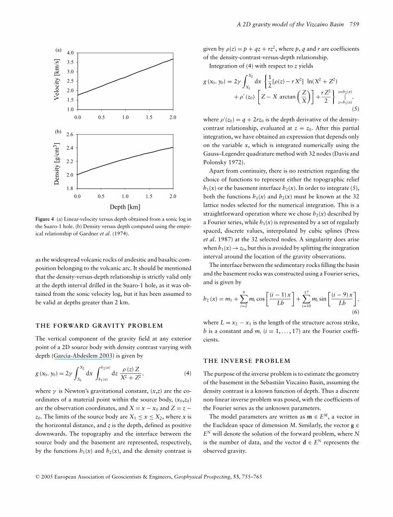
given by ρ(z) = p + qz + rz2, where p, q and r are coefficientsof the density-contrast-versus-depth relationship.

Integration of (4) with respect to z yields

g (x0, y0) = 2γ

∫ X2

X1

dx{

12

[ρ(z) − r X2] ln(X2 + Z2)

+ ρ ′ (z0)[

Z − X arctan(

ZX

)]+r Z2

2

}z=h2(x)

|z=h1(x)

,

(5)

where ρ ′(z0) = q + 2rz0 is the depth derivative of the density-contrast relationship, evaluated at z = z0. After this partialintegration, we have obtained an expression that depends onlyon the variable x, which is integrated numerically using theGauss–Legendre quadrature method with 32 nodes (Davis andPolonsky 1972).

Apart from continuity, there is no restriction regarding thechoice of functions to represent either the topographic reliefh1(x) or the basement interface h2(x). In order to integrate (5),both the functions h1(x) and h2(x) must be known at the 32lattice nodes selected for the numerical integration. This is astraightforward operation where we chose h2(x) described bya Fourier series, while h1(x) is represented by a set of regularlyspaced, discrete values, interpolated by cubic splines (Presset al. 1987) at the 32 selected nodes. A singularity does arisewhen h1(x) → z0, but this is avoided by splitting the integrationinterval around the location of the gravity observations.

The interface between the sedimentary rocks filling the basinand the basement rocks was constructed using a Fourier series,and is given by

h2 (x) = m1 +9∑

i=2

mi cos[

(i − 1) xLb

]+

17∑i=10

mi sin[

(i − 9) xLb

],

(6)

where L = x2 − x1 is the length of the structure across strike,b is a constant and mi (i = 1, . . . , 17) are the Fourier coeffi-cients.

T H E I N V E R S E P R O B L E M

The purpose of the inverse problem is to estimate the geometryof the basement in the Sebastian Vizcaıno Basin, assuming thedensity contrast is a known function of depth. Thus a discretenon-linear inverse problem was posed, with the coefficients ofthe Fourier series as the unknown parameters.

The model parameters are written as m ∈ EM, a vector inthe Euclidean space of dimension M. Similarly, the vector g ∈EN will denote the solution of the forward problem, where N

is the number of data, and the vector d ∈ EN represents theobserved gravity.

C© 2005 European Association of Geoscientists & Engineers, Geophysical Prospecting, 53, 755–765

760 J. Garcıa-Abdeslem et al.

The solution to the forward problem can be expressed as

g = G (m) w, (7)

where G(m) is an N × P matrix representing the integrandin (5), P is the number of integration nodes, and w is a P ×1 vector whose elements are the Gauss–Legendre weights fornumerical integration. The product, an N × 1 vector denotedby g, provides the numerical value that yields the gravity effect.

As the relationship between m and g in (7) is non-linear, theproblem must be linearized by expanding g to first order in aTaylor series around the point m0, which is an initial guess ofthe model parameters, i.e.

g = g(m0) + Jδm, (8)

where J is the N × M Jacobian matrix of partial derivativesof g with respect to the model parameters evaluated at m0,and δm = m − m0 is a parameter change vector representingthe perturbation in the parameters. It is assumed that an errorestimate σ i is associated with each datum, and further thatthe standard errors of the N data are statistically independent.Thus, a diagonal N × N weighting matrix S is defined as

S = diag[

1σ1

,1σ2

, · · · , 1σN

], (9)

and the perturbation δm is found by solving the system ofnormal equations given by

[λI + (SJ)TSJ] δm = (SJ)TS[d − g(m0)], (10)

where I is the identity matrix, T denotes transpose, and λ isreferred to as the damping factor.

Equation (10) is solved using LU decomposition, with for-ward elimination and back substitution. The iterative proce-dure follows the Marquardt–Levenberg algorithm: it consistsof first solving the forward problem for an initial trial valuem0, and once the Jacobian matrix has been obtained, the sys-tem of equations (10) is solved using an initial damping factorλ0, which is made proportional to the residual variance,

σ 2 = [Sd − Sg(m0)]T[Sd − Sg(m0)]N − M

, (11)

for N – M degrees of freedom, and a new solution is computedusing the vector relationship m1 = m0 + δm. If the residualvariance of the new solution is less than the previous one, anew solution m2 is sought, and this iterative process continuesuntil an acceptable solution is reached.

Partial derivatives

The elements of the Jacobian matrix are obtained by apply-ing Leibniz’s theorem for the differentiation of an integral(Abramowitz 1972, p. 11) to (5), i.e.

ddc

∫ b(c)

a(c)f (x, c) dx =

∫ b(c)

a(c)

∂

∂cf (x, c) dx

+ f (b, c)dbdc

− f (a, c)dadc

.

(12)

The integrand in (5) depends on the constant coefficients(the model parameters) in addition to the variable of integra-tion (x), and the limits of this integral are independent of theconstant coefficients. Therefore, with Leibniz’s theorem, thederivative of the integral with respect to the constant coeffi-cients is equivalent to integrating the partial derivative of theintegrand with respect to the model parameters. For example,if the basement interface h2(x) is given by a Fourier series withconstant coefficients mp(P = 1, . . . , M), such that

h2 (x) =∑

mp fp (x), (13)

where f p represents either sine or cosine terms, the partialderivatives of the gravity effect with respect to the coefficientsare

dg(x0, z0)dmp

= 2γ

∫ X2

X1

dx [h2(x) − z0]{

ρ (z0) − r X2

X2 + [h2 (x) − z0]2

+ ρ ′(z0) [h2(x) − z0]X2 + [h2(x) − z0]2

+ r}

fp(x). (14)

The integral above is computed using the same Gauss–Legendre quadrature method.

Sensitivity analysis

In order to assess the goodness of the solution and to estimateconfidence intervals for the parameters, a sensitivity analysiswas carried out by means of the resolution and covariancematrices, through singular-value decomposition (SVD) of thesensitivity matrix J, given by

J = U�VT, (15)

where U (N × M) and V (M × M) are the eigendata andeigenparameter matrices, and � (M × M) is a diagonal matrixcontaining the singular values or eigenvalues. The matrices Uand V are orthogonal, thus UT U = VT V = I. For the weightedand damped least-squares solution, the resolution matrix R isgiven by

R = V�2

(Λ + λI)2 VT. (16)

C© 2005 European Association of Geoscientists & Engineers, Geophysical Prospecting, 53, 755–765

A 2D gravity model of the Vizcaıno Basin 761

Through the resolution matrix we can express the solutionmk, obtained at iteration k, as a weighted average of the truesolution m with weights given by the row vectors of the matrixR, i.e.

mk = Rm. (17)

Thus, for perfect resolution, R should be the identity matrix,and solution mk is equal to the true solution. If the row vectorsof R have components spread around the diagonal terms, mk

represents a smoothed solution over the spread.A measure of the reliability of the solution is obtained from

the parameter covariance matrix, which is given by

C = σ 2 VΛ2

(Λ2 + λ2I

)2 VT, (18)

where σ 2 represents the residual variance at iteration k, forN − M degrees of freedom. The standard deviations of theparameter estimates are given by the square root of the diag-onal terms of the parameter covariance matrix.

R E S U LT S O F T H E G R AV I T Y I N V E R S I O N

The gravity profile, consisting of 165 data points spaced500 m apart, was interpreted assuming a density contrast thatdecreases with depth, as given by (3). The interface betweenthe sedimentary and basement rocks was represented by theFourier series given in (6), with X1 = 1 km and X2 = 83 km,corresponding to the end sides of the profile, and b = 5.

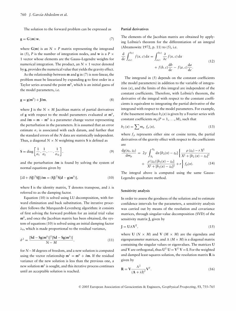
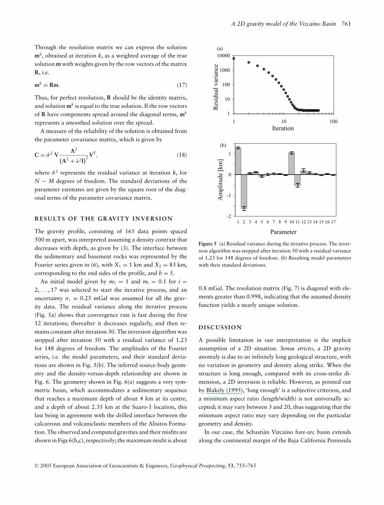
An initial model given by m1 = 1 and mi = 0.1 for i =2, . . . , 17 was selected to start the iterative process, and anuncertainty σ i = 0.25 mGal was assumed for all the grav-ity data. The residual variance along the iterative process(Fig. 5a) shows that convergence rate is fast during the first12 iterations; thereafter it decreases regularly, and then re-mains constant after iteration 30. The inversion algorithm wasstopped after iteration 50 with a residual variance of 1.23for 148 degrees of freedom. The amplitudes of the Fourierseries, i.e. the model parameters, and their standard devia-tions are shown in Fig. 5(b). The inferred source-body geom-etry and the density-versus-depth relationship are shown inFig. 6. The geometry shown in Fig. 6(a) suggests a very sym-metric basin, which accommodates a sedimentary sequencethat reaches a maximum depth of about 4 km at its centre,and a depth of about 2.35 km at the Suaro-1 location, thislast being in agreement with the drilled interface between thecalcareous and volcaniclastic members of the Alisitos Forma-tion. The observed and computed gravities and their misfits areshown in Figs 6(b,c), respectively; the maximum misfit is about

(a)

1

10

100

1000

10000

1 10 100

Iteration

Res

idua

l var

ianc

e

(b)

-2

-1

0

1

1 2 3 4 5 6 7 8 9 10 11 12 13 14 15 16 17

Parameter

Am

plit

ude

[km

]

Figure 5 (a) Residual variance during the iterative process. The inver-sion algorithm was stopped after iteration 50 with a residual varianceof 1.23 for 148 degrees of freedom. (b) Resulting model parameterswith their standard deviations.

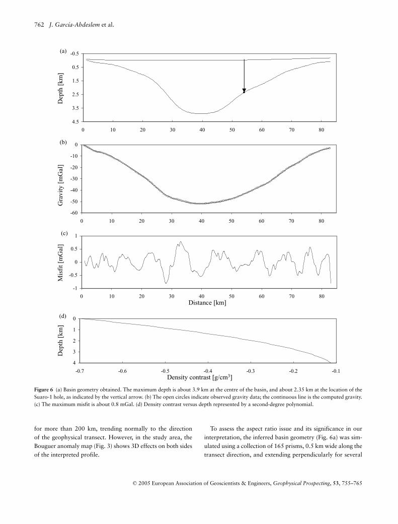
0.8 mGal. The resolution matrix (Fig. 7) is diagonal with ele-ments greater than 0.998, indicating that the assumed densityfunction yields a nearly unique solution.

D I S C U S S I O N

A possible limitation in our interpretation is the implicitassumption of a 2D situation. Sensu stricto, a 2D gravityanomaly is due to an infinitely long geological structure, withno variation in geometry and density along strike. When thestructure is long enough, compared with its cross-strike di-mension, a 2D inversion is reliable. However, as pointed outby Blakely (1995), ‘long enough’ is a subjective criterion, anda minimum aspect ratio (length/width) is not universally ac-cepted; it may vary between 3 and 20, thus suggesting that theminimum aspect ratio may vary depending on the particulargeometry and density.

In our case, the Sebastian Vizcaıno fore-arc basin extendsalong the continental margin of the Baja California Peninsula

C© 2005 European Association of Geoscientists & Engineers, Geophysical Prospecting, 53, 755–765

762 J. Garcıa-Abdeslem et al.

(a) -0.5

0.5

1.5

2.5

3.5

4.5

0 10 20 30 40 50 60 70 80

Dep

th[k

m]

(c)

-1

-0.5

0

0.5

1

0 10 20 30 40 50 60 70 80Distance [km]

Mis

fit [

mG

al]

(d) 0

1

2

3

4

-0.7 -0.6 -0.5 -0.4 -0.3 -0.2 -0.1Density contrast [g/cm3]

Dep

th[k

m]

(b)

-60

-50

-40

-30

-20

-10

0

0 10 20 30 40 50 60 70 80

Gra

vity

[mG

al]

Figure 6 (a) Basin geometry obtained. The maximum depth is about 3.9 km at the centre of the basin, and about 2.35 km at the location of theSuaro-1 hole, as indicated by the vertical arrow. (b) The open circles indicate observed gravity data; the continuous line is the computed gravity.(c) The maximum misfit is about 0.8 mGal. (d) Density contrast versus depth represented by a second-degree polynomial.

for more than 200 km, trending normally to the directionof the geophysical transect. However, in the study area, theBouguer anomaly map (Fig. 3) shows 3D effects on both sidesof the interpreted profile.

To assess the aspect ratio issue and its significance in ourinterpretation, the inferred basin geometry (Fig. 6a) was sim-ulated using a collection of 165 prisms, 0.5 km wide along thetransect direction, and extending perpendicularly for several

C© 2005 European Association of Geoscientists & Engineers, Geophysical Prospecting, 53, 755–765

A 2D gravity model of the Vizcaıno Basin 763

1 3 5 7 9 11 13 15 17

Parameter

1

3

5

7

9

11

13

15

17

Par

amet

er

0

0.1

0.2

0.3

0.4

0.5

0.6

0.7

0.8

0.9

Figure 7 (a) Resolution matrix after the 50th iteration, where thedamping parameter λ = 0.8542.

(a)

-60

-50

-40

-30

-20

-10

0

0 10 20 30 40 50 60 70 80

Distance [km]

Gra

vity

[mG

al]

L=200

L=10

(b )

-51.69

-51.66

-51.55

-51.16 -50.39 -49.23

0

50

100

150

200

250

L[k

m]

0.0

0.5

1.0

1.5

2.0

2.5

3.0

Gravity

difference[m

Gal]

Figure 8 (a) The gravity anomalies were computed by extending the basin geometry (Fig. 6a), obtained from the inversion, to distances L =200 km and L = 10 km on either side of the geophysical transect. (b) The grey rectangles represent the half-length of the source body alongstrike, and the numbers on top of them are the gravity values (mGal) computed at the centre of the profile (distance = 40 km). The solid circlesindicate the gravity differences, computed at the centre of the profile, between the model with L = 200 km, and the models for the other lengthsconsidered.

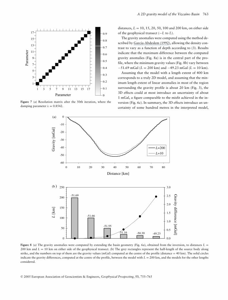
distances, L = 10, 15, 20, 50, 100 and 200 km, on either sideof the geophysical transect (−L to L).

The gravity anomalies were computed using the method de-scribed by Garcıa-Abdeslem (1992), allowing the density con-trast to vary as a function of depth according to (3). Resultsindicate that the maximum difference between the computedgravity anomalies (Fig. 8a) is in the central part of the pro-file, where the minimum gravity values (Fig. 8b) vary between−51.69 mGal (L = 200 km) and −49.23 mGal (L = 10 km).

Assuming that the model with a length extent of 400 kmcorresponds to a truly 2D model, and assuming that the min-imum length extent of linear anomalies in most of the regionsurrounding the gravity profile is about 20 km (Fig. 3), the3D effects could at most introduce an uncertainty of about1 mGal, a figure comparable to the misfit achieved in the in-version (Fig. 6c). In summary, the 3D effects introduce an un-certainty of some hundred metres in the interpreted model,

C© 2005 European Association of Geoscientists & Engineers, Geophysical Prospecting, 53, 755–765

764 J. Garcıa-Abdeslem et al.

assuming 2D geometry. Nonetheless, it can be considered as afirst step to a more comprehensive 3D interpretation.

C O N C L U S I O N S

The interpretation of gravity data over the Sebastian VizcaınoBasin was carried out along an 82-km-long profile that passedthrough the location of the Suaro-1 exploration hole, wherean available velocity-versus-depth relationship was used to de-rive a second-degree polynomial function to describe the den-sity contrast as a function of depth. The interpretation wasposed as a non-linear discrete inverse problem, constrainedby the density-versus-depth function. The inverted parame-ters are the coefficients of the Fourier series used to describethe geometry of the interface between the sedimentary andbasement rocks. The results of the inversion suggest that theSebastian Vizcaıno Basin accommodates a sedimentary se-quence reaching a maximum depth of about 4 km at its cen-tre. At the Suaro-1 location, the modelled basement is foundat 2.35 km, in agreement with the drilled interface betweencalcareous and volcaniclastic members of the Alisitos Forma-tion. The resolution matrix obtained in a sensitivity analysisstrongly suggests that the assumed density function leads to anearly unique solution.

A C K N O W L E D G E M E N T S

We thank Professor Dr E. Klingele, an anonymous reviewerand the Associate Editor Gokhan Ugurtas for their critical andhelpful reviews. We are also grateful to colleagues participat-ing in the fieldwork. In particular, we appreciate the collabo-ration of Cesar Jaques-Ayala (UNAM, Instituto de Geologıa,ERNO, Hermosillo Son.) and Mario Vega-Aguilar, who car-ried out the GPS survey, and Humberto Benitez and VictorFrıas, who drew the figures. We gratefully acknowledge fruit-ful conversations with Javier Helenes regarding the geologicalevolution of the Sebastian Vizcaıno region, and his review ofan early version of the original manuscript. The ‘Consejo Na-cional de Ciencia y Tecnologıa’ (CONACyT) provided finan-cial support for the project: grant No. 25792-T.

R E F E R E N C E S

Abramowitz M. 1972. Elementary analytical methods. In: Handbookof Mathematical Functions with Formulas, Graphs, and Mathemat-ical Tables (eds M. Abramowitz and I.A. Stegun), Chapter 3, pp.9–63. Dover Publications Inc.

Allison E.C. 1974. The type Alisitos formation (Cretaceous, Albian-Aptian) of Baja California, and its bivalve faunas. In: Geology of

Peninsular California (eds R.G. Gastil and J. Lillegraven), pp. 20–59. 49th Annual Meeting of American Association of PetroleumGeologists, Society of Economic Paleontologists and Mineralogists,Pacific Section, San Diego, CA.

Baldwin S.L. 1996. Contrasting P-T-t histories for blueschists fromthe western Baja Terrane and the Aegean: Effects of synsubductionexhumation and backarc extension. In: Subduction Top to Bottom(eds G.E. Bebout, D.W. Scholl, S.H. Kirby and J.P. Platt), pp. 135–141. Geophysical Monograph 96. American Geophysical Union.

Beal C.W. 1948. Reconnaissance of the Geology and Oil Possibili-ties of Baja California, Mexico. Memoir 31. Geological Society ofAmerica.

Blakely R.J. 1995. Potential Theory in Gravity and Magnetic Appli-cations. Cambridge University Press.

Castro-Leyva T.J., Delgado-Argote L.A. and Garcıa-Abdeslem J.2001. Geologıa y magnetometrıa del complejo mafico-ultramaficoPuerto Nuevo en el area de San Miguel, Penınsula de Vizcaıno, BajaCalifornia Sur. GEOS 21, 3–21.

Davis P.J. and Polonsky I. 1972. Numerical interpolation, differentia-tion and integration. In: Handbook of Mathematical Functions withFormulas, Graphs, and Mathematical Tables (eds M. Abramowitzand I.A. Stegun), Chapter 25, pp. 875–924. Dover Publications Inc.

Garcıa-Abdeslem J. 1992. Gravitational attraction of a rectangularprism with depth-dependent density. Geophysics 57, 470–473.

Garcıa-Abdeslem J. 2003. 2D modeling and inversion of gravity datausing density contrast varying with depth and source-basementgeometry described by the Fourier series. Geophysics 68, 1909–1916.

Garcıa-Abdeslem J. and Martın-Atienza B. 2001. A method to com-pute terrain corrections for gravimeter stations using a digital ele-vation model. Geophysics 66, 1110–1115.

Garcıa-Domınguez G. 1976. Prospeccion geologica en Baja Califor-nia. III. Simposium de Geologıa del Subsuelo, PEMEX, Superinten-dencia General de Exploracion, Distrito Frontera Norte, Reynosa,Tamaulipas, Mexico, pp. 31–49.

Gardner G.H.F., Gardner L.W. and Gregory A.R. 1974. Formationvelocity and density – The diagnostic basics for stratigraphic traps.Geophysics 39, 770–780.

Helenes J. 1984. Dinoflagellates from Cretaceous to early Tertiaryrocks of the Sebastian Vizcaıno basin, Baja California, Mexico. In:Geology of the Baja California Peninsula (ed. V.A. Frizzell), No. 39,pp. 89–106. Pacific Section, Society of Economic Paleontologistsand Mineralogists.

INEGI 1990. Red gravimetrica Mexicana, Aguascalientes, Mexico.Instituto Nacional de Estadıstica Geografıa e Informatica.

INEGI 1995. GEMA: Modelo digital de elevaciones, Aguascalientes,Mexico. Instituto Nacional de Estadıstica Geografıa e Informatica.

Levenberg K. 1944. A method for the solution of certain nonlinearproblems in least squares. Quarterly Journal of Applied Mathemat-ics 2, 164–168.

Lozano R.F. 1975. Evaluacion petrolıfera de la Penınsula de Baja Cal-ifornia, Mexico. Boletın de la Asociacion Mexicana de GeologosPetroleros 27, 104–329.

Marquardt D.W. 1970. Generalized inverses, ridge regression, biasedlinear estimation and nonlinear estimation. Technometrics 12, 591–612.

C© 2005 European Association of Geoscientists & Engineers, Geophysical Prospecting, 53, 755–765

A 2D gravity model of the Vizcaıno Basin 765

Mina U.F. 1957. Bosquejo geologico del Territorio de la Baja Califor-nia. Boletın de la Asociacion Mexicana de Geologos Petroleros 9,139–270.

Press W.H., Flannery B.P., Teukolsky S.A. and Vetterling W.T. 1987.Numerical Recipes. Cambridge University Press.

Ramos-Garcıa F. 1976. Prospeccion geofısica en la Penınsula de BajaCalifornia. III. Simposium de Geologıa del Subsuelo, PEMEX, Su-perintendencia General de Exploracion, Distrito Frontera Norte,Reynosa, Tamaulipas, Mexico, pp. 61–72.

Romo J.M., Garcıa-Abdeslem J., Gomez-Trevino E., EsparzaF. and Flores-Luna C. 2001. Resultados preliminaries

de un perfil geofısico a traves de la region central dela Penınsula de Baja California Mexico. GEOS 21, 96–107.

Sedlock R.L. 1996. Synsubduction forearc extension and blueschistsexhumation in Baja California, Mexico. In: Subduction Top toBottom (eds G.E. Bebout, D.W. Scholl, S.H. Kirby and J.P. Platt),pp. 155–162. Geophysical Monograph 96. American GeophysicalUnion.

Sedlock R.L., Ortega-Ramırez F. and Speed R.C. 1993. Tectonostrati-graphic Terranes and Tectonic Evolution of Mexico. Special Paper278. Geological Society of America.

C© 2005 European Association of Geoscientists & Engineers, Geophysical Prospecting, 53, 755–765