Ai

AD2

a

A

R

R

1

A

K

R

S

C

F

M

1

Tatmpcsmtt

0d

j o u r n a l o f m a t e r i a l s p r o c e s s i n g t e c h n o l o g y 2 0 6 ( 2 0 0 8 ) 263–274

journa l homepage: www.e lsev ier .com/ locate / jmatprotec

computational method to predict strip profilen rolling mills

rif S. Malik ∗, Ramana V. Grandhiepartment of Mechanical and Materials Engineering, Wright State University,09 Russ, 3640 Colonel Glenn Highway, Dayton, OH 45435, USA

r t i c l e i n f o

rticle history:

eceived 3 October 2007

eceived in revised form

9 November 2007

ccepted 6 December 2007

eywords:

olling mill

a b s t r a c t

Presented is a new computational method for predicting the static cross-sectional thickness

profile of rolled metal strip. Methods to model the strip profile and related flatness with

improved efficiency and accuracy remain central for achieving high quality flat-rolled prod-

ucts. The new method involves a novel combination of Timoshenko beam finite elements

with multiple coupled Winkler elastic foundations. It applies to simple mill configura-

tions, such as the common 4-high rolling mill, in addition to complex mill types, such

as the 20-high Sendzimir mill. The inherent benefits over traditional strip profile mod-

els include non-discrete elastic foundations, cubic displacement fields, rapid solution, and

mixed boundary conditions. The flexible nature of the model allows it to readily accommo-

trip profile

rown

latness

athematical model

date typical mechanisms used in industry to control strip profile, such as roll crowning,

roll bending, roll shifting, and roll crossing. Comparison of the predicted displacement

for a 4-high mill with that obtained using a large-scale finite element simulation pro-

vides validation of the presented strip profile calculation method for real-time industrial

applications.

of the rolled strip, and hence a non-uniform final thick-ness profile, as indicated for example in Fig. 1. Many factorsinfluence the evolution of a given strip profile, including themill configuration, operating loads, profile control devices,

. Introduction

o remain viable in a highly competitive global market, met-ls manufacturers must embrace new technologies to increasehe quality of rolled metal products, including steel, alu-

inum, titanium, copper, and brass. In response to this need,resented is a new mathematical method to efficiently cal-ulate the cross-sectional thickness profile of rolled metaltrip, an important dimensional quality attribute of flat-rolledetals. The new method is suitable for application with real-

ime computer systems for predicting and controlling the striphickness profile.

∗ Corresponding author. Tel.: +1 937 620 7329; fax: +1 937 775 5082.E-mail address: arif.malik@wright.edu (A.S. Malik).

924-0136/$ – see front matter © 2007 Elsevier B.V. All rights reserved.oi:10.1016/j.jmatprotec.2007.12.026

© 2007 Elsevier B.V. All rights reserved.

1.1. Dimensional quality requirements for rolled metalstrip

The rolling operation is characterized by incidental elasticdeflection of the mill housing, rolls, bearings, and other com-ponents occurring simultaneously with the elastic–plasticdeflection of the rolled strip. These combined deflections fre-quently lead to a non-uniform reduction in the thickness

264 j o u r n a l o f m a t e r i a l s p r o c e s s i n g t e c h n o l o g y 2 0 6 ( 2 0 0 8 ) 263–274

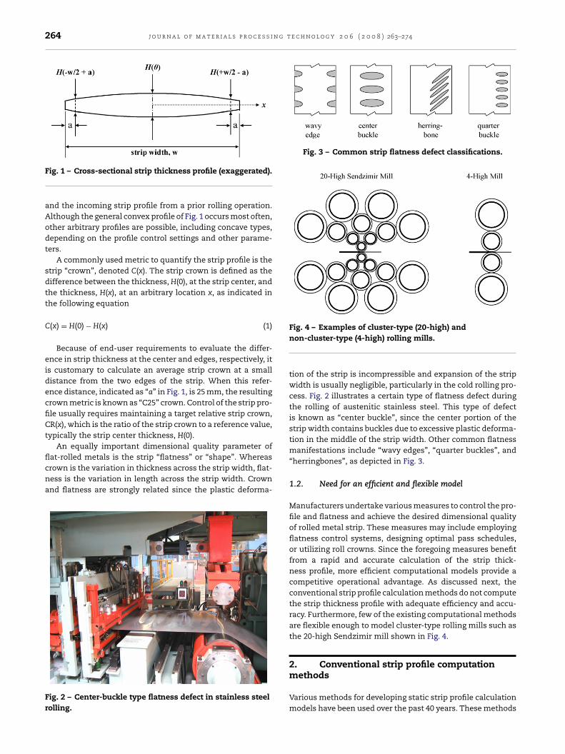
Fig. 3 – Common strip flatness defect classifications.

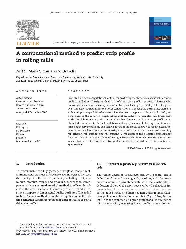
Fig. 1 – Cross-sectional strip thickness profile (exaggerated).

and the incoming strip profile from a prior rolling operation.Although the general convex profile of Fig. 1 occurs most often,other arbitrary profiles are possible, including concave types,depending on the profile control settings and other parame-ters.

A commonly used metric to quantify the strip profile is thestrip “crown”, denoted C(x). The strip crown is defined as thedifference between the thickness, H(0), at the strip center, andthe thickness, H(x), at an arbitrary location x, as indicated inthe following equation

C(x) = H(0) − H(x) (1)

Because of end-user requirements to evaluate the differ-ence in strip thickness at the center and edges, respectively, itis customary to calculate an average strip crown at a smalldistance from the two edges of the strip. When this refer-ence distance, indicated as “a” in Fig. 1, is 25 mm, the resultingcrown metric is known as “C25” crown. Control of the strip pro-file usually requires maintaining a target relative strip crown,CR(x), which is the ratio of the strip crown to a reference value,typically the strip center thickness, H(0).

An equally important dimensional quality parameter of

flat-rolled metals is the strip “flatness” or “shape”. Whereascrown is the variation in thickness across the strip width, flat-ness is the variation in length across the strip width. Crownand flatness are strongly related since the plastic deforma-

Fig. 2 – Center-buckle type flatness defect in stainless steelrolling.

Fig. 4 – Examples of cluster-type (20-high) andnon-cluster-type (4-high) rolling mills.

tion of the strip is incompressible and expansion of the stripwidth is usually negligible, particularly in the cold rolling pro-cess. Fig. 2 illustrates a certain type of flatness defect duringthe rolling of austenitic stainless steel. This type of defectis known as “center buckle”, since the center portion of thestrip width contains buckles due to excessive plastic deforma-tion in the middle of the strip width. Other common flatnessmanifestations include “wavy edges”, “quarter buckles”, and“herringbones”, as depicted in Fig. 3.

1.2. Need for an efficient and flexible model

Manufacturers undertake various measures to control the pro-file and flatness and achieve the desired dimensional qualityof rolled metal strip. These measures may include employingflatness control systems, designing optimal pass schedules,or utilizing roll crowns. Since the foregoing measures benefitfrom a rapid and accurate calculation of the strip thick-ness profile, more efficient computational models provide acompetitive operational advantage. As discussed next, theconventional strip profile calculation methods do not computethe strip thickness profile with adequate efficiency and accu-racy. Furthermore, few of the existing computational methodsare flexible enough to model cluster-type rolling mills such asthe 20-high Sendzimir mill shown in Fig. 4.

2. Conventional strip profile computation

methods

Various methods for developing static strip profile calculationmodels have been used over the past 40 years. These methods

t e c

mffieSm1Caecocratrbacp“iiiatetKttstwaitftam

whhsbmhbmmwdttmep

j o u r n a l o f m a t e r i a l s p r o c e s s i n g

ay be classified broadly as either: the single-beam on elasticoundation method (Stone and Gray, 1965); the influence coef-cient method (Shohet and Townsend, 1968, 1971; Hacquint al., 1994); the transport matrix method (Poplawski andeccombe, 1980; Guo, 1998); the pattern recognition/heuristicsethods (Hattori et al., 1993; Zhu et al., 1993; Jung and Im,

997); and the large-scale finite element method (Eibe, 1984;hen and Zhou, 1987). Although each method has uniquedvantages, none satisfies the combined requirements for anfficient, accurate, and flexible model capable of simulatingomplex mill configurations. Stone’s work studied the effectsf work roll bending and back-up roll bending to control striprown on 4-high rolling mills. In evaluating the effect of workoll bending on strip profile, Stone modeled the work roll assingle Euler–Bernoulli beam on a constant elastic founda-

ion that represented the mutual flattening between the workoll and the back-up roll. Hence, no independent shear orending deflection of the back-up roll was considered. Shohetnd Townsend’s influence coefficient method employs a dis-retized Green’s function to superpose the effects of multipleoint loads for the purpose of representing load distributions.Point matching” is utilized to satisfy equilibrium and compat-bility conditions at a finite number of discrete points along thenterfaces between the contacting rolls. The method assumesnitial arbitrary force distributions between contacting bodiesnd uses an iterative procedure to adjust the force distribu-ions to satisfy the point matching. Several improvements andnhancements have been made to this popular method overhe nearly four decades that it has been used. For instance,uhn and Weinstein (1970) modified the method to considerhe Poisson deflection due to axial bending stresses. Indenta-ion flattening at the interface between the work roll and thetrip was considered using Boussinesq’s theory by Kono (1983),hen by Tozawa (1984). Semi-empirical methods to model theork roll and strip interaction were employed by Nakajimand Matsumoto (1973). Matsubara et al. (1989) applied thenfluence coefficient method to predict the case of mutual con-act between upper and lower work rolls during the rolling ofoil. Gunawardene et al. (1981) used the method to solve forhe 20-high cluster mill using an equivalent stack of verticallyligned rolls, and Ogawa et al. (1991) extended the method toodel 12-high rolling mills.Due to the inherent complexity of cluster-type rolling mills,

hich have multiple roll contacting surfaces and require bothorizontal and vertical roll displacement calculations, thereave been far fewer instances of adapting the conventionaltrip crown models to them. For this reason, non-physics-ased models, derived from pattern recognition/heuristicsethods such as neural networks and fuzzy techniques,

ave been applied to cluster mills in greater relative num-ers. Although the influence coefficient method and transportatrix method have been used to simulate cluster-type rollingills in some cases, these methods lead to complex modelsith limited opportunity for industrial application. Anotherisadvantage of some conventional strip crown models is thatheir solution time is not sufficient for real-time mill con-

rol. The influence coefficient method, which has been the

ost widely studied, requires an iterative solution to satisfyquilibrium and compatibility conditions. Although the trans-ort matrix method was extended to cluster mills, because

h n o l o g y 2 0 6 ( 2 0 0 8 ) 263–274 265

of the large number of rolls and contact surfaces, it is notfast enough for real-time control (Guo and Malik, 2005). Thelarge-scale finite element method (FEM) is the most prohibitiveof all in terms of solution time because of the vast numberof elements required to model the narrow contact interfacesbetween adjacent rolls and between the working rolls andthe strip. Moreover, convergence difficulties associated withcontact-type structural FEM analyses pose additional solutionproblems.

The accuracy of the conventional methods may beexamined from a theoretical viewpoint. The pattern recogni-tion/heuristics models may be accurate if adequately trainedwith significant amounts of manufacturing data. The accuracyof both the influence coefficient method and the transportmatrix method depends on a large number of discretizationnodes. As accuracy is improved by increasing the node count,solution time also increases. Another factor adversely affect-ing the theoretical accuracy of the transport matrix methodis its use of discrete nodal springs to represent the contactinteractions between adjacent rolls and between the workingrolls and the strip. Cook et al. (2002) highlighted the risk ofusing discrete springs in lieu of continuous elastic foundationsand their particular difficulty in modeling contact interactionsnear component ends.

It is widely recognized that the rolling operation is dynamicin nature due to, for example, changes with respect to timeof yield stress, temperature, friction coefficient, rolling force,rolling speed, and geometric parameters of the strip. Despitethis, static models to predict the steady-state strip thick-ness profile, based on a “snapshot” of the input parameters,are widely used for pass-schedule setup and flatness controlsystems. In the case of pass-schedule setup, this circum-stance prevails because the pass-schedule calculations areused to assign nominal set-point values for thickness reduc-tions, rolling speed, and entry/exit tensions. Flatness controlalgorithms operate at command frequencies on the order of1 Hz—several orders of magnitude lower than the dynamicresponse of the mill to flatness actuation. The control fre-quencies for flatness control therefore render static transferfunctions sufficient. Thickness (gauge) control systems, on theother hand, operate at much higher frequencies and requireattention to the dynamic response. To account for the dynamicnature of the rolling operation when calculating the stripthickness profile, measured values of rolling parameters arecontinually applied to the static model in order to update thesteady-state thickness profile response. The method to predictstrip profile presented in this work employs a global stiffness-based linear system, and can therefore, if required, be usedtogether with an appropriate mass matrix to predict dynamicresponses of the rolling mill using well-known methods.

3. A new method to calculate strip crown

Presented is a new technique to model the static deflectionof the rolling mill components and compute the strip thick-

ness profile. The new method combines the conventionalfinite element method with analytical solid mechanics andis applicable to cluster-type mill configurations such as the20-high Sendzimir mill. In addition, it accommodates the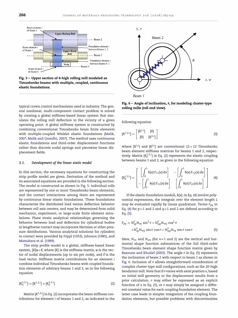

266 j o u r n a l o f m a t e r i a l s p r o c e s s i n g t e c h n o l o g y 2 0 6 ( 2 0 0 8 ) 263–274

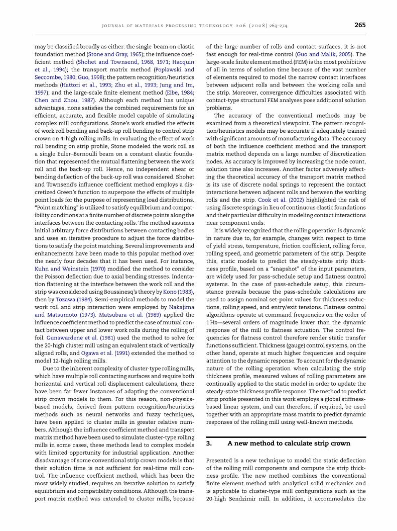
Fig. 5 – Upper section of 4-high rolling mill modeled asTimoshenko beams with multiple, coupled, continuous

function of x in Eq. (5), or � may simply be assigned a differ-

elastic foundations.

typical crown control mechanisms used in industry. The gen-eral nonlinear, multi-component contact problem is solvedby creating a global stiffness-based linear system that sim-ulates the rolling mill deflection in the vicinity of a givenoperating point. A global stiffness system is constructed bycombining conventional Timoshenko beam finite elementswith multiple-coupled Winkler elastic foundations (Malik,2007; Malik and Grandhi, 2007). The method uses continuouselastic foundations and third-order displacement functionsrather than discrete nodal springs and piecewise linear dis-placement fields.

3.1. Development of the linear static model

In this section, the necessary equations for constructing thestrip profile model are given. Derivation of the method andits associated equations are provided in the following section.The model is constructed as shown in Fig. 5: individual rollsare represented by one or more Timoshenko beam elements,and the contact interactions among them are representedby continuous linear elastic foundations. These foundationscharacterize the distributed load versus deflection behaviorbetween roll axis centers, and may be determined from solidmechanics, experiment, or large-scale finite element simu-lations. Plane strain analytical relationships governing thebehavior between load and deflection for cylindrical bodiesin lengthwise contact may incorporate Hertzian or other pres-sure distributions. Various analytical solutions for cylindersin contact were provided by Foppl (1933), Johnson (1985), andMatsubara et al. (1989).

The strip profile model is a global, stiffness-based linearsystem, [K]u = f, where [K] is the stiffness matrix, u is the vec-tor of nodal displacements (up to six per node), and f is theload vector. Stiffness matrix contributions for an element icombine individual Timoshenko beams with coupled founda-tion elements of arbitrary beams 1 and 2, as in the followingequation

[K1,2,iT ] = [K1,2,i] + [K1,2,i

F ] (2)

Matrix [K1,2,i] in Eq. (2) incorporates the beam stiffness con-tributions for element i of beams 1 and 2, as indicated in the

Fig. 6 – Angle of inclination, �, for modeling cluster-typerolling mills (roll end view).

following equation

[K1,2,i] =[

[K1,i] [0]

[0] [K2,i]

](3)

where [K1,i] and [K2,i] are conventional 12 × 12 Timoshenkobeam element stiffness matrices for beams 1 and 2, respec-tively. Matrix [K1,2,i

F ] in Eq. (2) represents the elastic couplingbetween beams 1 and 2, as given in the following equation

[K1,2,iF ] =

⎡⎢⎢⎣

[∫ L

0

k(x) F11(x) dx

]−

[∫ L

0

k(x) F12(x) dx

]

−[∫ L

0

k(x) F21(x) dx

] [∫ L

0

k(x) F22(x) dx

]⎤⎥⎥⎦ (4)

If the elastic foundation moduli, k(x), in Eq. (4) involve poly-nomial expressions, the integrals over the element length Lmay be evaluated rapidly by Gauss quadrature. Terms Fpq inEq. (4) for p = 1 and 2 and q = 1 and 2 are defined according toEq. (5):

Fpq = NTvpNvq sin2 � + NT

wpNwq cos2 �

+NTvpNwq sin � cos � + NT

wpNvq sin � cos � (5)

Here, Nvn and Nwn (for n = 1 and 2) are the vertical and hor-izontal shape function submatrices of the full third-orderTimoshenko beam element shape function matrix given byBazoune and Khulief (2003). The angle � in Eq. (5) representsthe inclination of beam 2 with respect to beam 1 as shown inFig. 6. Inclusion of � allows straightforward consideration ofcomplex cluster-type mill configurations, such as the 20-highSendzimir mill. Note that if � varies with axial position x, basedon initial mill geometry or the displacement results from aprior calculation, � may either be expressed as an explicit

ent constant value for each coupling foundation element. Thelatter case leads to simpler integration of the coupling foun-dation elements, but possible problems with discontinuities

t e c

wo

scaswpweofif

3

Cpdse

U

tmd

U

m

[

gebatdRlFac

taU

U

j o u r n a l o f m a t e r i a l s p r o c e s s i n g

hen using large nodal spacing and large changes in the valuef � between elements.

In the presented method, degrees of freedom u repre-enting lateral (axial) displacement of the rolls and strip areonstrained. For the case of large strip width to thickness ratio,s in cold rolling processes, the lateral displacement of thetrip is usually so small it is neglected. In hot rolling processes,here the strip width to thickness ratio is lower, lateral slip-ing of the strip usually occurs near its edges in the form ofidth expansion. With regard to the strip profile, the width

xpansion has the effect of reducing the foundation modulif the strip, k(x), near its edges. The effect of slip on strip pro-le is thus accounted for by the presented method since theoundation modulus k can be a function of x.

.2. Derivation of the linear static model

onsider a single beam of unit width and length L in the x–ylane on a fixed Winkler elastic foundation. For a given y-isplacement field, v(x), the additional potential energy of theystem, UF, due to the elastic foundation is provided by Cookt al. (2002) and is restated in the following equation

F = 12

∫ L

0

k(x) v(x)2 dx (6)

Since the continuous displacement function, v(x), is equalo the product of the vertical displacement shape function

atrix, Nv(x), and the y-direction nodal displacement vector,

v, the foundation energy UF can be written as

F = 12

dTv

∫ L

0

k(x) NTv Nv dx dv (7)

The corresponding Winkler foundation element stiffnessatrix contribution, [KFv], is

KFv] =∫ L

0

k(x) NTv Nv dx (8)

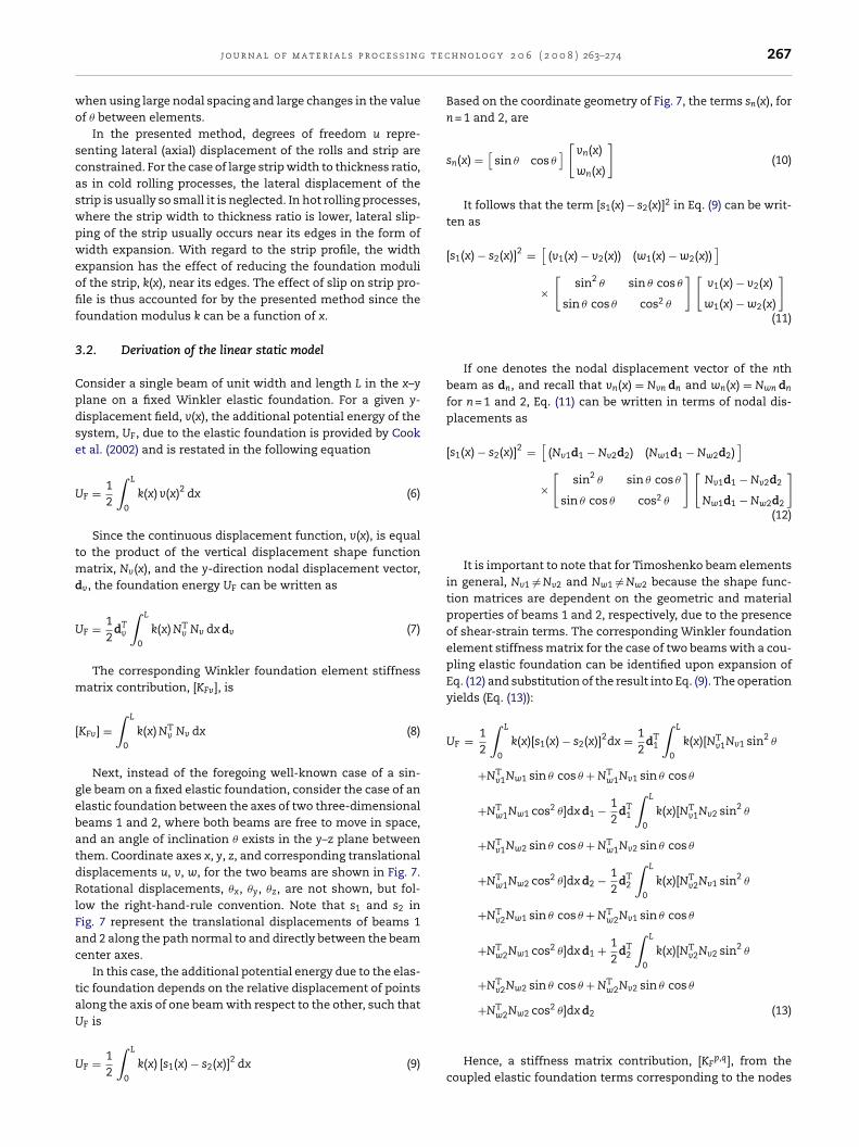
Next, instead of the foregoing well-known case of a sin-le beam on a fixed elastic foundation, consider the case of anlastic foundation between the axes of two three-dimensionaleams 1 and 2, where both beams are free to move in space,nd an angle of inclination � exists in the y–z plane betweenhem. Coordinate axes x, y, z, and corresponding translationalisplacements u, v, w, for the two beams are shown in Fig. 7.otational displacements, �x, �y, �z, are not shown, but fol-

ow the right-hand-rule convention. Note that s1 and s2 inig. 7 represent the translational displacements of beams 1nd 2 along the path normal to and directly between the beamenter axes.

In this case, the additional potential energy due to the elas-ic foundation depends on the relative displacement of pointslong the axis of one beam with respect to the other, such that

F is

F = 12

∫ L

0

k(x) [s1(x) − s2(x)]2 dx (9)

h n o l o g y 2 0 6 ( 2 0 0 8 ) 263–274 267

Based on the coordinate geometry of Fig. 7, the terms sn(x), forn = 1 and 2, are

sn(x) =[

sin � cos �][

vn(x)

wn(x)

](10)

It follows that the term [s1(x) − s2(x)]2 in Eq. (9) can be writ-ten as

[s1(x) − s2(x)]2 =[

(v1(x) − v2(x)) (w1(x) − w2(x))]

×[

sin2 � sin � cos �

sin � cos � cos2 �

][v1(x) − v2(x)

w1(x) − w2(x)

]

(11)

If one denotes the nodal displacement vector of the nthbeam as dn, and recall that vn(x) = Nvn dn and wn(x) = Nwn dn

for n = 1 and 2, Eq. (11) can be written in terms of nodal dis-placements as

[s1(x) − s2(x)]2 =[

(Nv1d1 − Nv2d2) (Nw1d1 − Nw2d2)]

×[

sin2 � sin � cos �

sin � cos � cos2 �

][Nv1d1 − Nv2d2

Nw1d1 − Nw2d2

]

(12)

It is important to note that for Timoshenko beam elementsin general, Nv1 �= Nv2 and Nw1 �= Nw2 because the shape func-tion matrices are dependent on the geometric and materialproperties of beams 1 and 2, respectively, due to the presenceof shear-strain terms. The corresponding Winkler foundationelement stiffness matrix for the case of two beams with a cou-pling elastic foundation can be identified upon expansion ofEq. (12) and substitution of the result into Eq. (9). The operationyields (Eq. (13)):

UF = 12

∫ L

0

k(x)[s1(x) − s2(x)]2dx = 12

dT1

∫ L

0

k(x)[NTv1Nv1 sin2 �

+NTv1Nw1 sin � cos � + NT

w1Nv1 sin � cos �

+NTw1Nw1 cos2 �]dx d1 − 1

2dT

1

∫ L

0

k(x)[NTv1Nv2 sin2 �

+NTv1Nw2 sin � cos � + NT

w1Nv2 sin � cos �

+NTw1Nw2 cos2 �]dx d2 − 1

2dT

2

∫ L

0

k(x)[NTv2Nv1 sin2 �

+NTv2Nw1 sin � cos � + NT

w2Nv1 sin � cos �

+NTw2Nw1 cos2 �]dx d1 + 1

2dT

2

∫ L

0

k(x)[NTv2Nv2 sin2 �

+NTv2Nw2 sin � cos � + NT

w2Nv2 sin � cos �

+NT N cos2 �]dx d (13)

w2 w2 2

Hence, a stiffness matrix contribution, [KFp,q], from the

coupled elastic foundation terms corresponding to the nodes

268 j o u r n a l o f m a t e r i a l s p r o c e s s i n g t

Fig. 7 – Coordinate system for displacements betweenbeams 1 and 2.

between the two beams p and q can be identified as

[Kp,qF ] = (−1)p+q

∫ L

0

k(x)[NTvpNvq sin2 � + NT

vpNwq sin � cos �

+NTwpNvq sin � cos � + NT

wpNwq cos2 �]dx (14)

3.3. Elastic foundation moduli

The elastic foundation moduli, k(x), of Eqs. (4) and (14) rep-resent linear spring-constants between the adjacent rolls(beams). Unlike in a conventional finite element approach, inwhich a large number of very small elements may be requiredto adequately model the contact interface between the rolls,the elastic foundations used here represent the “aggregate”displacement–load relationship between the roll axis centers.

A similar approach to represent the metal strip as dis-crete linear springs was made by Guo (1986) in his transportmatrix method. In examining rolling data for 1880 mm widemild steel at up to 80% thickness reduction, Guo found theuse of a linear “strip modulus” satisfactory. In the presentedmethod, the same concept of a strip modulus is used, but thediscrete nodal springs are replaced with a continuous elasticfoundation function.

3.4. Representation of strip profile control devices

Parameters affecting the final strip profile during rolling maybe classified as either controllable or non-controllable. Non-controllable factors include the initial strip profile, diameterprofiles ground onto the rolls, and the incidental effects of rollwear and roll thermal expansion. Because the elastic foun-dation moduli, k(x), of Eqs. (4) and (14) are functions of beamaxial position x, they take into account the non-controllablestrip profile factors. Controllable factors include roll bending,roll shifting, and roll crossing mechanisms. Shifting and cross-ing mechanisms are modeled with the presented method byadjusting the model geometry and modifying the elastic foun-dation modulus accordingly. Roll bending is accommodated by

providing corresponding load values to the forcing vector f.

Although the analytical plane-strain and elastic half-spacesolutions for the flattening between rolls do not account forthe length-to-diameter ratio of the rolls, nor for any specific

e c h n o l o g y 2 0 6 ( 2 0 0 8 ) 263–274

axial loading position, these effects are accommodated by theelastic foundation moduli since they are indeed functions ofaxial position x. Zhou et al. compared the classical analyti-cal formulae for contact between rolls with three-dimensionalfinite element simulations using a traction boundary condi-tion on a single roll (Zhou et al., 1996). They noted variousdifferences between the FEM solutions and the classic solu-tions when studying the effects of strip width, roll diameterto length ratio, and rolling load intensity. Hacquin also stud-ied roll end effects upon enhancement of Berger’s strip profilemodel, which was an improved version of Shohet’s originalinfluence coefficient model (Hacquin et al., 1998; Berger et al.,1976). These noted geometric effects on the flattening charac-teristics between rolls are accommodated by the foundationstiffness moduli formulation of the presented method.

3.5. Strip crown calculation

To calculate the strip crown by Eq. (1), the vertical position,y(x), of the common generator surface between the strip andthe work roll at the desired axial location x must first be com-puted. The common generator vertical position, y(x), betweenarbitrary beams 1 and 2 can be obtained using Eq. (15):

y(x) = y1j(x) +(

D1(x)2

− k(x)k1(x)

I(x)

)sin � (15)

where y1j(x) is the vertical position for node j at the axial coor-dinate x of beam 1 (in this case the strip). The term D1(x) is theoriginal diameter of beam 1, which in this case refers to thestrip thickness. Term k(x) is the equivalent foundation mod-ulus between beam 1 and the adjacent beam (upper or lowerwork roll), and k1(x) is the foundation stiffness contribution ofbeam 1, which is the strip modulus. The term I(x) in Eq. (15)represents the total interference between the adjacent beams,as determined from the original nodal coordinates, the rolldiameter profiles, and the nodal displacements. Eq. (15) canbe derived from a free body diagram of the nodes connect-ing beam 1 and the adjacent beam, noting that the ratio ofthe foundation displacement magnitudes is the inverse of theratio of the foundation stiffness moduli:

�1(x)�(x)

= k(x)k1(x)

(16)

In Eq. (16), �1(x) is the magnitude of the displacement of thefoundation modulus k1(x) between the surface and the axis ofbeam 1, and �(x) is the magnitude of the displacement of theequivalent foundation modulus k(x) between the axis of beam1 and the axis of the adjacent beam.

4. Model validation using finite elementanalysis

4.1. Application of new method to 4-high mill

The new method is now applied to simulate the deflection ina 4-high rolling mill and compare the predicted strip profilewith that obtained using a large-scale, commercial finite ele-ment analysis (FEA) package. Partial symmetry of the 4-high

j o u r n a l o f m a t e r i a l s p r o c e s s i n g t e c h n o l o g y 2 0 6 ( 2 0 0 8 ) 263–274 269

Table 1 – Geometry parameters for 4-high mill

Geometry parameter Value

Strip entry thickness, H (mm) 25.400Strip center exit thickness, h (mm) 21.077Strip width, w (mm) 508.00Work roll diameter, Dw (mm) 254.00Work roll length, Lw (mm) 1270.0Backup roll diameter, Db (mm) 508.00Backup roll length, Lb (mm) 1270.0

Table 2 – Parameters for application of new model to4-high mill

Model parameter Value

Strip foundation modulus, ˇ (N/mm2) 13,790Strip foundation modulus modification

length, d (mm)25.00

Strip foundation modulus end nodesratio, f1

0.50

Backup roll boundary condition type onend nodes

Pinned

Work roll boundary condition type onend nodes

Free

Strip lower edge vertical displacementboundary condition (mm)

6.35

Backup roll elastic modulus, Eb (GPa) 206.84Backup roll Poisson ratio, �b 0.30

roT

hahaend(

(ten

Table 3 – Results summary for application of new modelto 4-high mill

New model result Value

Strip center thickness, h (mm) 21.077Strip C25 thickness, hc25 (mm) 19.959

vertical displacement results is now made using the commer-

Work roll elastic modulus, Ew (GPa) 206.84Work roll Poisson ratio, �w 0.30Number of Timoshenko beam elements 48

oll configuration is exploited, leading to an upper half modelf the mill. Dimensions of the mill components are shown inable 1.

Table 2 indicates model parameters for simulating the 4-igh mill. A total of 48 Timoshenko beam elements withssociated coupling foundations are used to model the upperalf of the mill. The strip foundation modulus, k(x), is assignedconstant value, ˇ = 13790 N/mm2, over the strip width, w,

xcept for a modification to decrease the foundation stiff-ess beginning at points x = ±x0, corresponding to a distance,, from either strip edge. The magnitude of x0 is thereforew/2–d).

The specific assignment of k(x) is indicated in Eqs. (17a) and17b). The parameter f in Eq. (17b) represents the fraction of

1

he nominal strip foundation modulus ˇ remaining at the stripdges x = ±w/2. A value of 0.5 is intuitively used for f1, since theodes at x = ±w/2 equally share an interior foundation modu-

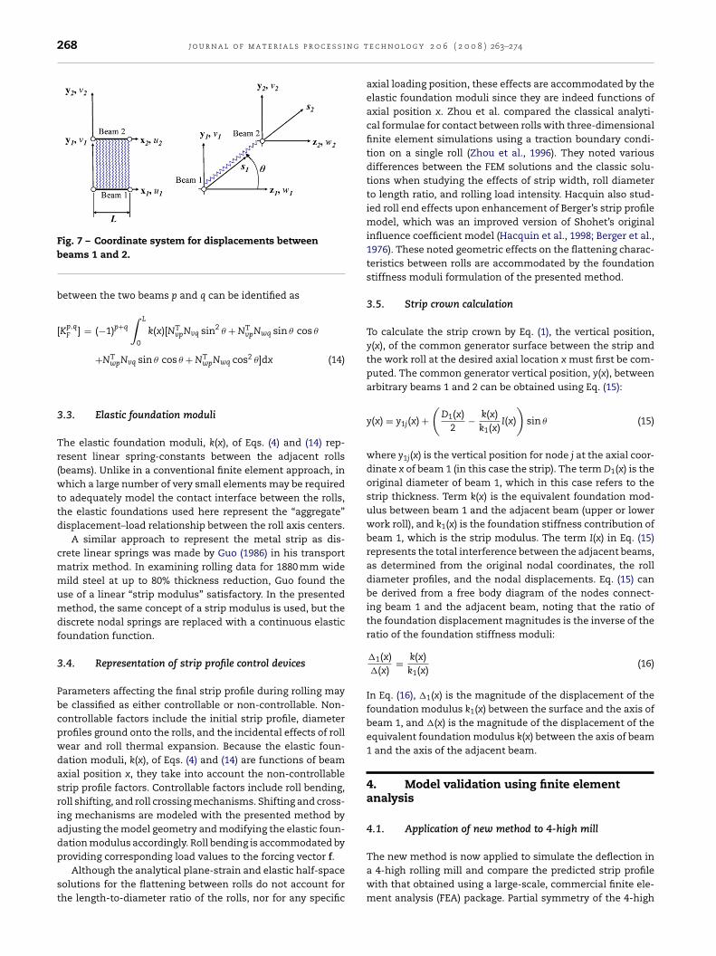
Fig. 8 – Contact force distribution (a) and uppe

Strip crown, C25 (mm) 1.118Strip crown, C25 (%) 5.304Total force, F (MN) 33.949

lus ˇ and no external foundation. These equations provide aparabolic decrease in k(x) from a value of ˇ at x = ±x0 to a valueof 0.5ˇ at x = ±w/2.

k(x) = ˇ, |x| < x0 (17a)

k(x) = ˇ

[f1 − 1

d2|x − x0|2 + 1

], |x| ≥ x0 (17b)

Fig. 8a illustrates the resulting contact force distribution atthe interface between the strip and the upper work roll, andbetween the upper work roll and the upper back-up roll. Fig. 8bshows the thickness profile of the upper half of the strip rel-ative to the semi-thickness at the strip edge. By Eq. (1), thestrip crown C(x) corresponding to C25 locations (x = ±229 mm)is 1.118 mm, since the semi-thickness is 0.559 mm greater atthe strip center than at the C25 edge locations. Table 3 sum-marizes the results for the 4-high mill simulation. The modelpredicts that for a 17.02% reduction in thickness at the stripcenter, the thickness at a distance of 25 mm from either edge ofthe strip is 1.118 mm less than the center thickness (19.959 mmvs. 21.077 mm). Hence, the C25 strip crown is 1.118 mm, or5.304% of the center thickness.

Since this simulation includes no crown control devices,Fig. 8a and b illustrates the typical deflection and load char-acteristics that occur in a 4-high rolling mill. It can be seenthat the increase in the contact force distribution in the vicin-ity of the strip edges leads to greater corresponding thicknessreduction in those areas.

4.2. ABAQUS finite element solution of 4-high mill

To evaluate the ability of the new method to accurately predictthe deflection behavior in a 4-high mill, a comparison of the

cial finite element analysis package ABAQUS (Version 6.6-1).Due to the computational expense of contact-type structuralanalyses in conventional FEA, all planes of symmetry for the

r strip semi-thickness relative to edge (b).

270 j o u r n a l o f m a t e r i a l s p r o c e s s i n g t e c h n o l o g y 2 0 6 ( 2 0 0 8 ) 263–274

of 4

obtained. Note that because of the strip crown phenomenon,the strip thickness reduction, �y, in the following equation,represents the average reduction over the width of the strip to

Table 4 – Parameters for application of ABAQUS FEA to4-high mill

ABAQUS FEA model parameter Value

Strip foundation modulus, ˇ (N/mm2) 13790Strip average thickness reduction, �y (mm) 4.94Average contact dimension, b (mm) 25.06Strip area foundation modulus, ˇA (N/mm3) 550.4Strip equivalent elastic modulus, E (N/mm2) 15,300

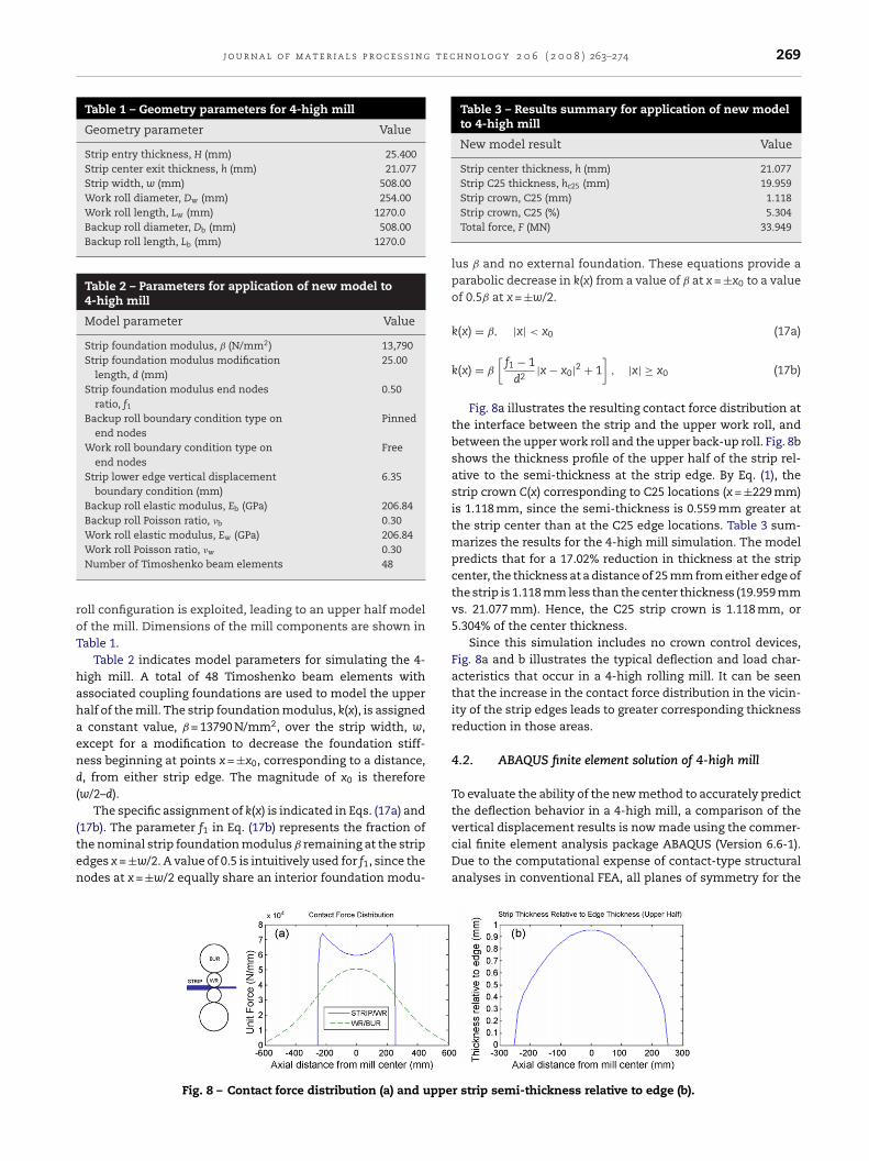
Fig. 9 – ABAQUS FEA model of upper section

rolling mill are exploited, leading to the 1/8th model of the4-high mill shown in Fig. 9. Over 64,000 three-dimensionaltetrahedral elements are generated as a result of the extrememesh refinement assigned automatically by ABAQUS at thecontact interfaces between the rolls and strip.

Rather than performing an elastic–plastic analysis, elasticparameters are assigned to the strip elements in the ABAQUSFEA model such that they represent a one-dimensional linearelastic foundation. The purpose is to obtain a direct com-parison for validating the new model. This is accomplishedby assigning specific values to the Poisson ratio, �, and theYoung’s (elastic) modulus, E, of the strip.

Assuming a constant foundation modulus, k(x) = ˇ, and not-ing that this modulus is equivalent to the spring constant perunit strip width w, the following expression can be obtained foran area modulus ˇA, where ˇA = ˇ/b, and A = bw is the contactarea between the strip and the work roll.

ˇA = F/�y

A(18)

In Eq. (18), F is the total load applied to the strip, �y is thefoundation displacement (strip thickness reduction), and A isthe foundation area. Hooke’s law for the y-direction strain,corresponding to the strip thickness reduction, is

εy = 1E

[�y − v(�x + �z)] (19)

In Eq. (19), εy is the true strain; E is the elastic modulus; v

is the Poisson ratio; and �x, �y, �z are the average orthogonalstress components. Next, a zero Poisson ratio is assigned toachieve one-dimensional behavior of the strip foundation, andone may note that the true strain, εy, may be written in termsof the ratio of the thickness reduction, which is simply theengineering strain. One can therefore write Eq. (19) as

ln(

1 + �y)

= �y(20)

H E

In Eq. (20), H is the initial strip thickness. Since averagestress �y is equal to F/A, one can substitute F from Eq. (18) intoEq. (20) and rearrange to obtain an expression for the elastic

-high mill (64,054 3D tetrahedral elements).

modulus, E, in terms of the specified area foundation modulus,ˇA.

E = ˇA�y

ln(1 + �y/H)(21)

The engineering strain may be used directly to obtain Eq.(22) if the strip thickness reduction is less than 10%:

E = ˇAH (22)

To validate the new method with the results of the ABAQUSFEA model, a zero Poisson ratio and an equivalent elastic mod-ulus, E, using Eq. (21) or (22) are assigned to the strip elementsof the FEA model. To determine the equivalent elastic modulusfor the strip upper half, one need only use half the initial stripthickness and half the thickness reduction, but twice the foun-dation modulus in Eqs. (21) and (22). Substituting the data fromSection 4.1 into Eq. (21), and estimating contact dimensionb using Eq. (23) for rigid rolls (Roberts, 1978), an equiva-lent approximate strip elastic modulus, E = 15,300 N/mm2, forthe tetrahedral elements of the strip upper half section is

ABAQUS Version 6.6-1 element library type(3D tetrahedral)

CD310M

Number of 3D tetrahedral elements 64,054Friction conditions (all contact interfaces) Frictionless

j o u r n a l o f m a t e r i a l s p r o c e s s i n g t e c h n o l o g y 2 0 6 ( 2 0 0 8 ) 263–274 271

Table 5 – Vertical displacement comparison between ABAQUS FEA and new model

Model type No. of elements Strip center disp. (mm) Strip C25 disp. (mm) Strip edge disp. (mm)

FEA iter 1 44,716 4.3896 3.7315 3.36503.6640 3.31473.5884 3.24083.6316 3.1521

o

b

am(batawp

AcimrFacipb

ot

FEA iter 2 42,672 4.2718FEA iter 3 64,054 4.2459New Model 48 4.1891

btain an average contact dimension b:

=√

Dw�y

2(23)

The parameter values used for the ABAQUS FEA modelre shown in Table 4. All other parameters for the 4-highill example, including boundary conditions, are the same

Table 2). It should be noted that the contact interfacesetween the work roll and back-up roll, and between the stripnd the work roll, are assigned frictionless conditions. In con-rast, the new method does not allow for any sliding betweendjacent components. As a result, the ABAQUS FEA solutionill yield substantially different results for the strip thicknessrofile if sliding is an important influential factor.

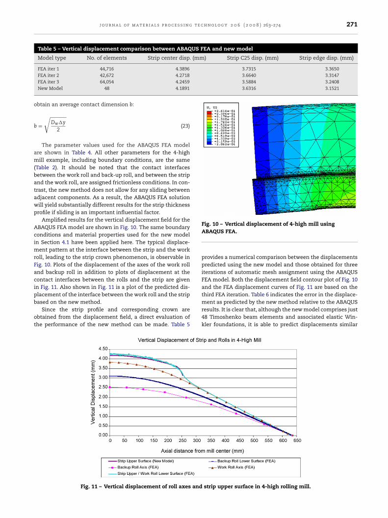
Amplified results for the vertical displacement field for theBAQUS FEA model are shown in Fig. 10. The same boundaryonditions and material properties used for the new modeln Section 4.1 have been applied here. The typical displace-

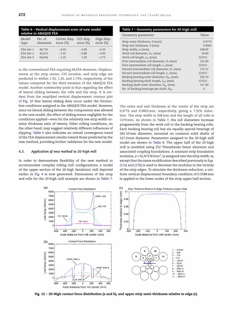
ent pattern at the interface between the strip and the workoll, leading to the strip crown phenomenon, is observable inig. 10. Plots of the displacement of the axes of the work rollnd backup roll in addition to plots of displacement at theontact interfaces between the rolls and the strip are givenn Fig. 11. Also shown in Fig. 11 is a plot of the predicted dis-lacement of the interface between the work roll and the strip

ased on the new method.

Since the strip profile and corresponding crown arebtained from the displacement field, a direct evaluation ofhe performance of the new method can be made. Table 5

Fig. 11 – Vertical displacement of roll axes and

Fig. 10 – Vertical displacement of 4-high mill usingABAQUS FEA.

provides a numerical comparison between the displacementspredicted using the new model and those obtained for threeiterations of automatic mesh assignment using the ABAQUSFEA model. Both the displacement field contour plot of Fig. 10and the FEA displacement curves of Fig. 11 are based on thethird FEA iteration. Table 6 indicates the error in the displace-

ment as predicted by the new method relative to the ABAQUSresults. It is clear that, although the new model comprises just48 Timoshenko beam elements and associated elastic Win-kler foundations, it is able to predict displacements similar

strip upper surface in 4-high rolling mill.

272 j o u r n a l o f m a t e r i a l s p r o c e s s i n g t e c h n o l o g y 2 0 6 ( 2 0 0 8 ) 263–274

Table 6 – Vertical displacement error of new modelrelative to ABAQUS FEA

Modeltype

No. ofelements

Center disp.error (%)

C25 disp.error (%)

Edge disp.error (%)

FEA iter 1 44,716 −4.59 −2.68 −6.33

Table 7 – Geometry parameters for 20-high mill

Geometry parameter Value

Strip entry thickness, H (mm) 0.9779Strip exit thickness, h (mm) 0.9063Strip width, w (mm) 508.00Work roll diameter, Dw (mm) 50.80Work roll length, Lw (mm) 1270.0First intermediate roll diameter, Df (mm) 101.60First intermediate roll length, Lf (mm) 1270.0Second intermediate roll diameter, Ds (mm) 172.72Second intermediate roll length, Ls (mm) 1270.0Backing bearing outer diameter, Dbb (mm) 292.10Backing bearing shaft length, Lbb (mm) 1270.0Backing shaft outer diameter, Dbs (mm) 127.00

FEA iter 2 42,672 −1.95 −0.88 −4.90FEA iter 3 64,054 −1.35 1.20 −2.73

to the conventional FEA requiring 64,054 elements. Displace-ments at the strip center, C25 location, and strip edge arepredicted to within 1.35, 1.20, and 2.73%, respectively, of thevalues computed for the third iteration of the ABAQUS FEAmodel. Another noteworthy point is that regarding the effectof lateral sliding between the rolls and the strip. It is evi-dent from the amplified vertical displacement contour plotof Fig. 10 that lateral sliding does occur under the friction-less conditions assigned in the ABAQUS FEA model. However,since no lateral sliding between the components was allowedin the new model, the effect of sliding seems negligible for theconditions applied—even for the relatively low strip width-to-entry thickness ratio of twenty. Other rolling conditions, onthe other hand, may suggest relatively different influences ofslipping. Table 6 also indicates an overall convergence trendof the FEA displacement results toward those predicted by thenew method, providing further validation for the new model.

4.3. Application of new method to 20-high mill

In order to demonstrate flexibility of the new method to

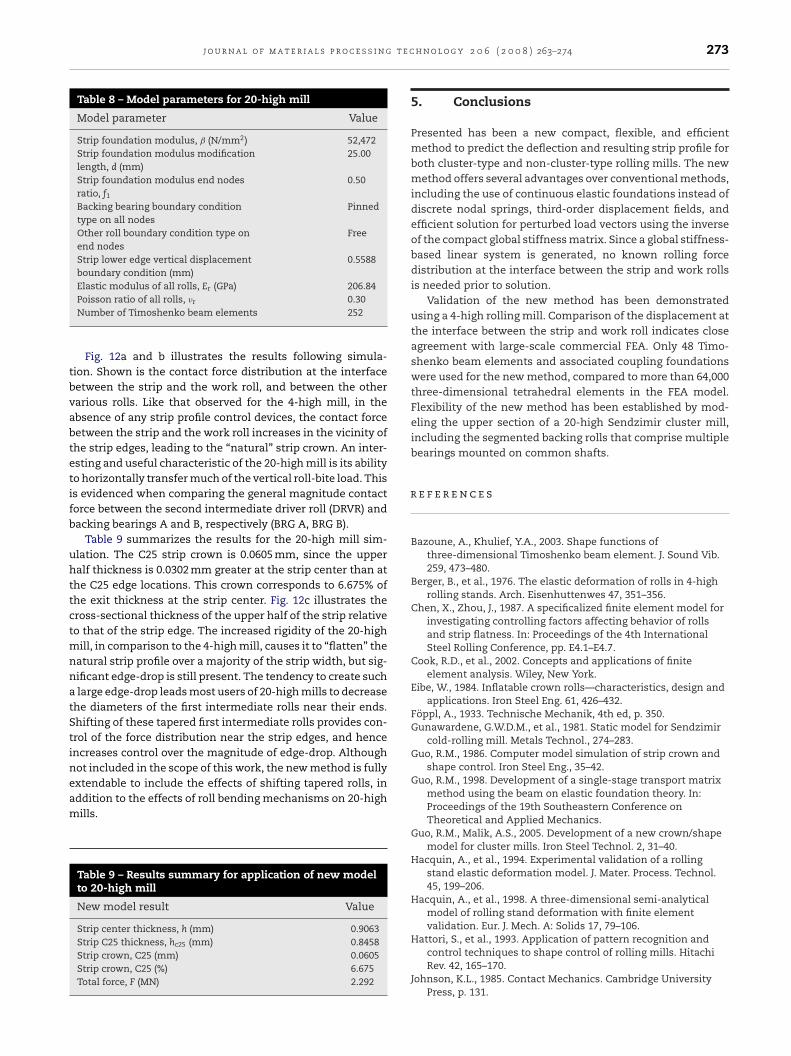
accommodate complex rolling mill configurations, a modelof the upper section of the 20-high Sendzimir mill depictedearlier in Fig. 4 is now generated. Dimensions of the stripand rolls for the 20-high mill example are shown in Table 7.

Fig. 12 – 20-High contact force distribution (a and b), a

No. of backing bearings per shaft, Nbb 6

The entry and exit thickness at the center of the strip are0.9779 and 0.9063 mm, respectively, giving a 7.32% reduc-tion. The strip width is 508 mm and the length of all rolls is1270 mm. As shown in Table 7, the roll diameters increaseprogressively from the work roll to the backing bearing rolls.Each backing bearing roll has six equally spaced bearings of292.10 mm diameter, mounted on common solid shafts of127.0 mm diameter. Parameters assigned to the 20-high millmodel are shown in Table 8. The upper half of the 20-highmill is modeled using 252 Timoshenko beam elements andassociated coupling foundations. A constant strip foundationmodulus, ˇ = 52,472 N/mm2, is assigned over the strip width, w,except that the same modification described previously in Eqs.(17a) and (17b) is used to decrease the modulus in the vicinity

of the strip edges. To simulate the thickness reduction, a uni-form vertical displacement boundary condition of 0.5588 mmis applied to the lower nodes of the strip upper half section.

nd upper strip semi-thickness relative to edge (c).

j o u r n a l o f m a t e r i a l s p r o c e s s i n g t e c

Table 8 – Model parameters for 20-high mill

Model parameter Value

Strip foundation modulus, ˇ (N/mm2) 52,472Strip foundation modulus modificationlength, d (mm)

25.00

Strip foundation modulus end nodesratio, f1

0.50

Backing bearing boundary conditiontype on all nodes

Pinned

Other roll boundary condition type onend nodes

Free

Strip lower edge vertical displacementboundary condition (mm)

0.5588

Elastic modulus of all rolls, Er (GPa) 206.84

tbvabtetifb

uhttctmnnatStineam

r

Poisson ratio of all rolls, �r 0.30Number of Timoshenko beam elements 252

Fig. 12a and b illustrates the results following simula-ion. Shown is the contact force distribution at the interfaceetween the strip and the work roll, and between the otherarious rolls. Like that observed for the 4-high mill, in thebsence of any strip profile control devices, the contact forceetween the strip and the work roll increases in the vicinity ofhe strip edges, leading to the “natural” strip crown. An inter-sting and useful characteristic of the 20-high mill is its abilityo horizontally transfer much of the vertical roll-bite load. Thiss evidenced when comparing the general magnitude contactorce between the second intermediate driver roll (DRVR) andacking bearings A and B, respectively (BRG A, BRG B).

Table 9 summarizes the results for the 20-high mill sim-lation. The C25 strip crown is 0.0605 mm, since the upperalf thickness is 0.0302 mm greater at the strip center than athe C25 edge locations. This crown corresponds to 6.675% ofhe exit thickness at the strip center. Fig. 12c illustrates theross-sectional thickness of the upper half of the strip relativeo that of the strip edge. The increased rigidity of the 20-high

ill, in comparison to the 4-high mill, causes it to “flatten” theatural strip profile over a majority of the strip width, but sig-ificant edge-drop is still present. The tendency to create suchlarge edge-drop leads most users of 20-high mills to decrease

he diameters of the first intermediate rolls near their ends.hifting of these tapered first intermediate rolls provides con-rol of the force distribution near the strip edges, and hencencreases control over the magnitude of edge-drop. Althoughot included in the scope of this work, the new method is fully

xtendable to include the effects of shifting tapered rolls, inddition to the effects of roll bending mechanisms on 20-highills.

Table 9 – Results summary for application of new modelto 20-high mill

New model result Value

Strip center thickness, h (mm) 0.9063Strip C25 thickness, hc25 (mm) 0.8458Strip crown, C25 (mm) 0.0605Strip crown, C25 (%) 6.675Total force, F (MN) 2.292

h n o l o g y 2 0 6 ( 2 0 0 8 ) 263–274 273

5. Conclusions

Presented has been a new compact, flexible, and efficientmethod to predict the deflection and resulting strip profile forboth cluster-type and non-cluster-type rolling mills. The newmethod offers several advantages over conventional methods,including the use of continuous elastic foundations instead ofdiscrete nodal springs, third-order displacement fields, andefficient solution for perturbed load vectors using the inverseof the compact global stiffness matrix. Since a global stiffness-based linear system is generated, no known rolling forcedistribution at the interface between the strip and work rollsis needed prior to solution.

Validation of the new method has been demonstratedusing a 4-high rolling mill. Comparison of the displacement atthe interface between the strip and work roll indicates closeagreement with large-scale commercial FEA. Only 48 Timo-shenko beam elements and associated coupling foundationswere used for the new method, compared to more than 64,000three-dimensional tetrahedral elements in the FEA model.Flexibility of the new method has been established by mod-eling the upper section of a 20-high Sendzimir cluster mill,including the segmented backing rolls that comprise multiplebearings mounted on common shafts.

e f e r e n c e s

Bazoune, A., Khulief, Y.A., 2003. Shape functions ofthree-dimensional Timoshenko beam element. J. Sound Vib.259, 473–480.

Berger, B., et al., 1976. The elastic deformation of rolls in 4-highrolling stands. Arch. Eisenhuttenwes 47, 351–356.

Chen, X., Zhou, J., 1987. A specificalized finite element model forinvestigating controlling factors affecting behavior of rollsand strip flatness. In: Proceedings of the 4th InternationalSteel Rolling Conference, pp. E4.1–E4.7.

Cook, R.D., et al., 2002. Concepts and applications of finiteelement analysis. Wiley, New York.

Eibe, W., 1984. Inflatable crown rolls—characteristics, design andapplications. Iron Steel Eng. 61, 426–432.

Foppl, A., 1933. Technische Mechanik, 4th ed, p. 350.Gunawardene, G.W.D.M., et al., 1981. Static model for Sendzimir

cold-rolling mill. Metals Technol., 274–283.Guo, R.M., 1986. Computer model simulation of strip crown and

shape control. Iron Steel Eng., 35–42.Guo, R.M., 1998. Development of a single-stage transport matrix

method using the beam on elastic foundation theory. In:Proceedings of the 19th Southeastern Conference onTheoretical and Applied Mechanics.

Guo, R.M., Malik, A.S., 2005. Development of a new crown/shapemodel for cluster mills. Iron Steel Technol. 2, 31–40.

Hacquin, A., et al., 1994. Experimental validation of a rollingstand elastic deformation model. J. Mater. Process. Technol.45, 199–206.

Hacquin, A., et al., 1998. A three-dimensional semi-analyticalmodel of rolling stand deformation with finite elementvalidation. Eur. J. Mech. A: Solids 17, 79–106.

Hattori, S., et al., 1993. Application of pattern recognition andcontrol techniques to shape control of rolling mills. HitachiRev. 42, 165–170.

Johnson, K.L., 1985. Contact Mechanics. Cambridge UniversityPress, p. 131.

n g t

274 j o u r n a l o f m a t e r i a l s p r o c e s s i

Jung, J.Y., Im, Y.T., 1997. Simulation of fuzzy shape control forcold-rolled strip with randomly irregular strip shape. J. Mater.Process. Technol. 63 (1–3), 248.

Kono, T., 1983. Development of a mathematical model on crowncontrol in strip rolling. Sumitomo Search 28, 1–8.

Kuhn, H.A., Weinstein, A.S., 1970. Lateral distribution of pressurein thin strip rolling. J. Eng. Ind. ASME, 453–456.

Malik, A.S., Rolling mill optimization using an accurate and rapidnew model for mill deflection and strip thickness profile, PhDDissertation, Wright State University, Dayton, OH, 2007.

Malik, A.S., Grandhi, R.V., Analytical method for use inoptimizing dimensional quality in hot and cold rolling mills,US Patent Application No. 11,686,381,2007.

Matsubara, S., et al., 1989. Optimization of work roll taper for

extremely thin strip rolling. ISIJ Int. 29, 58–63.

Nakajima, K., Matsumoto, H., 1973. Proceedings of 24th JapaneseJoint Conference for Technology of Plasticity, JSTP 29.

Ogawa, S., et al., 1991. Prediction of flatness of fine gauge striprolled by 12-high cluster mill. ISIJ Int. 31, 599–606.

e c h n o l o g y 2 0 6 ( 2 0 0 8 ) 263–274

Poplawski, J.V., Seccombe, D.A., 1980. Bethlehem’s contribution tothe mathematical modeling of cold rolling in tandem mills.AISE Yearbook, 391–402.

Roberts, W.L., 1978. Cold Rolling of Steel. Marcel Dekker, NewYork, p. 484.

Shohet, K.N., Townsend, N.A., 1968. Roll bending methods ofcrown control in four-high plate mills. J. Iron Steel Inst.,1088–1098.

Shohet, K.N., Townsend, N.A., 1971. Flatness control in platerolling. J. Iron Steel Inst., 769–775.

Stone, M.D., Gray, R., 1965. Theory and practice aspects in crowncontrol. Iron Steel Eng. Yearbook, 1965, 657–667.

Tozawa, Y., 1984. Analysis for three-dimensional deformation instrip rolling taken deformation of the rolls into consideration.In: Proceedings of the Conference of Advanced Technology of

Plasticity, Tokyo, pp. 1151–1160.

Zhou, S., et al., 1996. Influence of roll geometry and strip widthon flattening in flat rolling. Steel Res. 67, 200–204.

Zhu, H.T., et al., 1993. A fuzzy algorithm for flatness control in ahot strip mill. J. Mater. Process. Technol. 140, 123–128.