Am. axup Hyt., Vol. 41. No. 4. pp 467-484, 1997© 1997 British Occupation*! Hygiene Society. All rights reserved

Published by Hsevier Saence LtdPrinted m Gnat Britain

0003-4878/97 517.00 + 0 00

PII: S0003-^878(97)00007-0

A COMPREHENSIVE STRATEGY FOR THE ASSESSMENT OFNOISE EXPOSURE AND RISK OF HEARING IMPAIRMENT

J. Malchaire and A. Piette["Catholic University of Louvain, Work andPhysiology UnitJcios Chapelle-aux-Champs 3038,I— B-1200JBrussels, Belgium!

(Received 14 November 1996)

Abstract—A comprehensive strategy is presented for the evaluation of the daily noise exposurelevel [i-EX,d 'n dB(A)] and the assessment of the risk of hearing impairment. The nsk is denned asthe probability for a worker with a given exposure history to noise to develop a hearing deficitabove a given threshold. It is shown that for a given accuracy to be obtained on the risk prediction,the precision required on the Z-EX,d ' s low at levels around 90 dB(A) and increases at higher levels.The strategy uses the concepts of homogeneous group of exposure (HGE) and stationarity interval(S.I.), defined as the period over which the exposure distribution is the same for the members of theHGE. The number of workers to sample, the number of samples to take for each worker and theirduration are discussed. A semi-random sampling is recommended, excluding the periods with lownoise exposure. Tests are proposed for the homogeneity of the group and the validity of the S.I.. Acorrected standard deviation is defined in order to take into account the skewness of thedistribution of the noise equivalent levels of the samples and formulas are presented to estimate the^-Ex.d. l t s standard error and the corresponding nsk of hearing impairment, © 1997 BritishOccupational Hygiene Society. Published by Elsevier Saence Ltd — '

INTRODUCTION

The literature concerning the sampling strategies to chemical agents is veryextensive. Many papers have been published concerning the validity of the conceptof a 'representative day' (Olsen and Jensen, 1994), the variations between and withinsubjects (Rappaport et al., 1993) and the accuracy of the estimation of the averageexposure level (Rappaport and Selvin, 1987; Attfield and Hewett, 1992).

Some papers have been published dealing with the same problems in other fields,in particular concerning the exposure of workers to risks of low back pain (Burdorf,1993, 1995).

During a roundtable (No. 218) at the 1996 conference of the American IndustrialHygiene Association, all the presentations clearly showed that these concepts are nottaken into account in the field of noise. As the American and other internationalregulations require an estimate to be made of the noise exposure by means of thedaily noise exposure level [LEX.CI in dB(A)], it is usually concluded that the noiselevel must be measured over an 8-h shift. This was the practice recommended by allthe speakers. Royster, in his presentation, took some liberties with this rule andrecommended recording the noise level over 4 h . . . in order to speed up theevaluation process and decrease the cost of the measurement campaign. No onementioned the concept of 'homogeneous exposure groups' nor discussed therepresentativity of a shift, chosen at random, nor questioned the normality of thedistribution of the noise levels.

467

by guest on July 15, 2011annhyg.oxfordjournals.org

Dow

nloaded from

468 J Malchaire and A. Piette

The present article proposes a comprehensive method for noise exposureassessment with a discussion of the alternative objectives of such an assessment, anew definition of the risk of deafness and appropriate statistical tools to test thevalidity of the hypotheses of homogeneity, stationarity and normality of the data. Itis based mainly on concepts available in the literature and was validated using adatabase of 10 8-h continuous recordings of 1 min equivalent levels at 22 differentworkplaces. An example of application of the method is given in Appendix A and avalidation study is described in Appendix B.

RISK OF DEAFNESS

The risk of deafness can be defined as the percentage of the population ofworkers of a given age who, after a given history of exposure to noise (years ofexposure and corresponding LEX|d) would develop a hearing deficit greater than agiven threshold.

This percentage can be computed following the procedure described in the ISOstandard 1999 (1990) entitled "Determination of the occupational noise exposure andestimation of the noise induced hearing impairment", the information needed being

— the age A of the person (years);—his noise exposure history: this can be described by the sequence of exposures

during his working life, that is, the set of consecutive durations of exposure T,and the corresponding daily noise exposure levels LEx,d,'>

—the frequencies from which to compute the mean hearing deficit: for example,the frequencies of 1, 2 and 3 kHz;

— the threshold of mean hearing deficit considered as constituting a significantimpairment for the worker;o a handicap threshold above which significant interference with communica-

tion occurs, namely 35 dB in average at the three chosen frequencies;o a disability threshold above which significant interference with the daily life

and work capacity occurs, namely 50 dB average at the three chosenfrequencies, as adopted in Belgium.

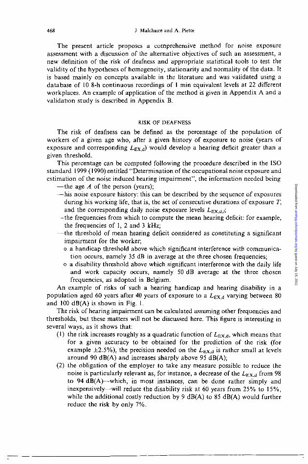
An example of risks of such a hearing handicap and hearing disability in apopulation aged 60 years after 40 years of exposure to a LEX,d varying between 80and 100 dB(A) is shown in Fig. 1.

The risk of hearing impairment can be calculated assuming other frequencies andthresholds, but these matters will not be discussed here. This figure is interesting inseveral ways, as it shows that:

(1) the risk increases roughly as a quadratic function of LEX>d, which means thatfor a given accuracy to be obtained for the prediction of the risk (forexample ±2.5%), the precision needed on the L^.d is rather small at levelsaround 90 dB(A) and increases sharply above 95 dB(A);

(2) the obligation of the employer to take any measure possible to reduce thenoise is particularly relevant as, for instance, a decrease of the LEX,d from 98to 94 dB(A)—which, in most instances, can be done rather simply andinexpensively—will reduce the disability risk at 60 years from 25% to 15%,while the additional costly reduction by 9 dB(A) to 85 dB(A) would furtherreduce the risk by only 7%.

by guest on July 15, 2011annhyg.oxfordjournals.org

Dow

nloaded from

Assessment of noise exposure and risk of hearing impairment 469

10

102 104

Fig. 1. Risk of occupational hearing impairment as a function of the daily noise exposure level (percentageof the population aged 60 years after 40 years of exposure to noise, suffering from an hearing impairment

greater than 35 or 50 dB average at 1, 2 and 3 kHz).

OBJECTIVES OF RISK ASSESSMENT

Three different objectives can be pursued in the evaluation of exposure to noise.The first is to identify the major noise sources in order effectively to control the

noise. This is, indeed, the primary objective of a hearing conservation programmebut requires an evaluation procedure rather different from the two others as it willrely mainly on, for example, point measurements, frequency analyses andreverberation time measurements in order to characterize the factors responsiblefor the emission and propagation of the noise.

The second objective is to comply with the law. As, typically, occupationalexposure limits of 85 and 90 dB(A) are prescribed by regulations, the mainobjective, in many exposure assessment cases, is to determine whether the L^x.a ' s

well below 85 dB(A), between 85 and 90 dB(A), or well above 90 dB(A).Paradoxically, it does not much matter whether the LEX,d is 93 or 96 dB(A) for

instance, as, in either cases, the exposure is unacceptable and control measures(usually hearing protection) must be implemented. By contrast, in this philosophy,more measurements will be taken in order to determine, with a sufficient accuracy,whether the Z-Ex.d is above or below 85 or 90 dB(A).

This objective, implicitly or explicitly pursued in most cases, would be acceptableif the control measures were working and the hearing protectors were effectivelyprotecting the workers. It is obvious that this is not the case and therefore thisapproach, although fulfilling the legal requirements, has little interest.

The third objective, which is much more exacting, is to attempt to identify, assoon as possible during their professional life, those subjects who are likely todevelop hearing deficits that will significantly impair their quality of life. Thisrequires accurate evaluations of their noise exposure and their hearing deficits(through a rigorous audiometric programme).

The present paper will describe and justify a comprehensive strategy for the

by guest on July 15, 2011annhyg.oxfordjournals.org

Dow

nloaded from

470 J. Malchaire and A. Piette

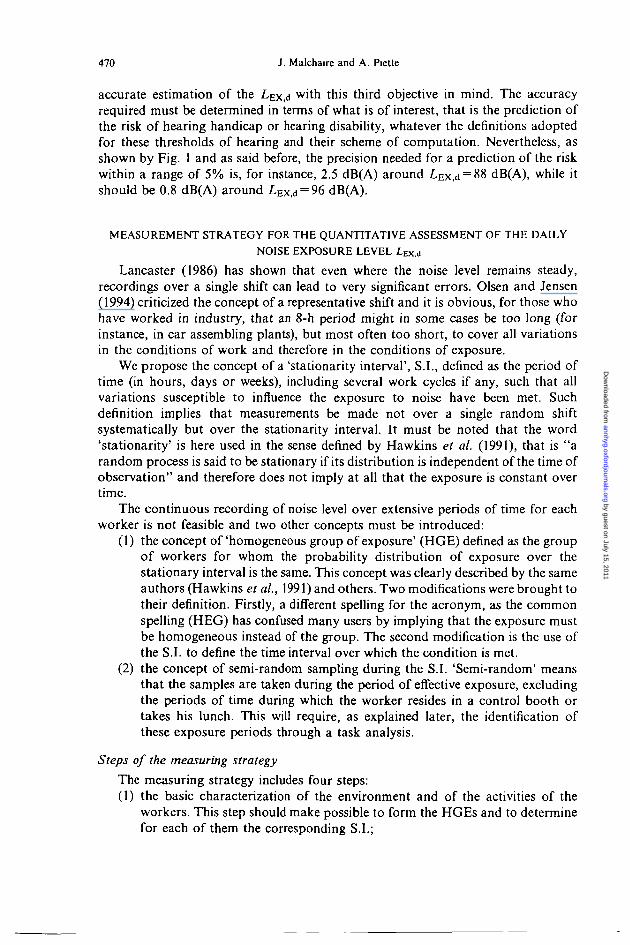
accurate estimation of the LEX.CI with this third objective in mind. The accuracyrequired must be determined in terms of what is of interest, that is the prediction ofthe risk of hearing handicap or hearing disability, whatever the definitions adoptedfor these thresholds of hearing and their scheme of computation. Nevertheless, asshown by Fig. 1 and as said before, the precision needed for a prediction of the riskwithin a range of 5% is, for instance, 2.5 dB(A) around LEx,d = 88 dB(A), while itshould be 0.8 dB(A) around LEx,d = 96 dB(A).

MEASUREMENT STRATEGY FOR THE QUANTITATIVE ASSESSMENT OF THE DAILY

NOISE EXPOSURE LEVEL i.£x.d

Lancaster (1986) has shown that even where the noise level remains steady,recordings over a single shift can lead to very significant errors. Olsen and Jensen(1994) criticized the concept of a representative shift and it is obvious, for those whohave worked in industry, that an 8-h period might in some cases be too long (forinstance, in car assembling plants), but most often too short, to cover all variationsin the conditions of work and therefore in the conditions of exposure.

We propose the concept of a 'stationarity interval', S.I., denned as the period oftime (in hours, days or weeks), including several work cycles if any, such that allvariations susceptible to influence the exposure to noise have been met. Suchdefinition implies that measurements be made not over a single random shiftsystematically but over the stationarity interval. It must be noted that the word'stationarity' is here used in the sense denned by Hawkins et al. (1991), that is "arandom process is said to be stationary if its distribution is independent of the time ofobservation" and therefore does not imply at all that the exposure is constant overtime.

The continuous recording of noise level over extensive periods of time for eachworker is not feasible and two other concepts must be introduced:

(1) the concept of 'homogeneous group of exposure' (HGE) defined as the groupof workers for whom the probability distribution of exposure over thestationary interval is the same. This concept was clearly described by the sameauthors (Hawkins et al., 1991) and others. Two modifications were brought totheir definition. Firstly, a different spelling for the acronym, as the commonspelling (HEG) has confused many users by implying that the exposure mustbe homogeneous instead of the group. The second modification is the use ofthe S.I. to define the time interval over which the condition is met.

(2) the concept of semi-random sampling during the S.I. 'Semi-random' meansthat the samples are taken during the period of effective exposure, excludingthe periods of time during which the worker resides in a control booth ortakes his lunch. This will require, as explained later, the identification ofthese exposure periods through a task analysis.

Steps of the measuring strategyThe measuring strategy includes four steps:(1) the basic characterization of the environment and of the activities of the

workers. This step should make possible to form the HGEs and to determinefor each of them the corresponding S.I.;

by guest on July 15, 2011annhyg.oxfordjournals.org

Dow

nloaded from

Assessment of noise exposure and risk of hearing impairment 471

(2) the qualitative evaluation of the exposure, which concludes the first step andprovides a first estimate of the Z-Ex.d, through conventional procedures;

(3) the detailed measurements themselves; and(4) the quantitative evaluation of the results and the estimation of the LEX,d, and

of its precision.It must be emphasized that this is only one part, but a significant one, of the

hearing conservation programme, as audiometric and noise control programmesmust also be developed.

The present paper will focus on steps 3 and 4 of this strategy, as step 1 has beenadequately described and illustrated among others by Hawkins et al. (1991) and step2 is amply discussed by Royster et al. (1986), along with all the conditions to be metfor the calibration of the instruments and the general organizing of the measurementcampaign.

Planification of the measurements

At the end of steps 1 and 2, HGE groups have been formed, the correspondingS.I. denned and the periods of effective exposure during the S.I. identified.

Let us define—n H G E as the number of workers belonging to a given HGE;—the series of T/Q and Tn defining the times (in min) at the beginning and at the

end of the sequence /' of effective exposure to noise;— r o = the stationarity interval expressed in min: ( = 480xS.I. in case of 8-h shifts);— Ti = 53(r,i — TJO), the total time of effective exposure to noise (in min);— T2=TQ—T\, the total time during which the worker is exposed to a noise level

^Aeq2 vvell below [20 dB(A) at least] those met during T\ (in min).The questions to answer before performing the sampling campaign are:

On how many workers nw among the T\HGE should the sampling be conducted?. Onestep in the interpretation will be to verify whether the group is indeed homogeneous.Therefore a sufficiently large number of workers must be chosen, to be able to observethe potential heterogeneity. Table 1 gives the number of workers n^ to take intoconsideration in order to be sure at 95% that one of the workers from the 20% of the«HGE who would be the most exposed (Leidel et al., 1977) is included in the sample.

How many samples to take per worker?. The same reasoning as above can beadopted: the number of sample ns per worker being chosen in order to increase theprobability of encountering the noisiest conditions. Based on the approach of Leidelet al. (1977), it can be shown that five samples would be enough to be sure at 90%that one sampling period is taken during the 33% of the time with the highest noiselevel. This number n, = 5 could therefore be used systematically. Our experienceshows that this leads to a standard error of the LEX,d which in most cases is smaller

Table 1

"HOE

. Number

< 6

of workers

7-8

IE 6

W to

9-11

7

sample as a functionexposure

12-14 15-18

8 9

ot the size

19-26

10

of the homogeneous

27-43 44-50

11 12

group of

>50

14

by guest on July 15, 2011annhyg.oxfordjournals.org

Dow

nloaded from

472 J. Malchaire and A. Piette

than 1 dB(A). As discussed before, this is not needed in all cases and in particularfor LEX.CI lower than 90 dB(A). The recommended procedure is therefore to startrather arbitrarily with ns = 3 samples per workers, to go through the measuringcampaign and the interpretation and to collect additional samples per person, ifneeded to reach the desired precision on the

What should be the duration of the samples?. According to our study reported inAppendix B, the accuracy of the LEx,d varies roughly as a function of the number ofsamples, but as a function of the square root of the sample duration At. Therefore, itappears preferable to increase n, and use short samples. The problem is not critical,however, if the Larsen (1971) philosophy is used, assuming that the standard deviationof the noise equivalent levels (LAeq) obtained from samples of duration AT2 can beestimated from the standard deviation of the LAeq values for samples of duration ATi.

The mathematical expression proposed by Larsen (1971) in the field ofatmospheric pollution has proved to be invalid in the field of noise and our study(Appendix B) showed that a better prediction can be obtained using the followingexpression:

A r 'Y3 '—j

sIn particular this expression will be used to derive the standard deviation for a 8-hperiod.

As this estimation is possible, At should be determined according to practicalconsiderations. Samples of short duration would be possible in industries with shortworkcycles but would be impractical, the time spent to install the instrumentationbecoming relatively too important compared to the sampling time. In the commoncase of workplaces with no particular cycle time, At of the order of 30—60 minappears to be most practical.

When to schedule the sampling? n,nw samples of duration At must be scheduledat random over a period of a stationarity interval and during the phases of effectiveexposure to noise (duration T\). This can be done using a table of random numbers.

Let r, be the ith random number, r,. T\ indicates the time during the period ofeffective noise exposure when the sampling should start.

From the list of (T/o, Tn) defined previously, the time of the start of the samplingcan be easily determined.

It remains to be verified whether a sample of duration AT can be taken duringthis sequence after the starting time and whether this scheduling is not in conflictwith a previous scheduled sample. If this is the case, this random number is droppedand the computation restarted with the next one.

How to sample?. Two different measuring techniques have been used in the past:the zonal method and the ambulatory method. The zonal method was proposed asthe most cost-effective method by Rockwell (1983). It consists of locating anintegrating sound level meter at a point near the worker. This method provides moreaccurate noise measurements (no or minimum interference with the frequency

by guest on July 15, 2011annhyg.oxfordjournals.org

Dow

nloaded from

Assessment of noise exposure and risk of hearing impairment 473

response of the microphone) but the results are often not representative of the realexposure of the worker.

Dosimeters are attached to the subjects with the microphone placed near the ear.Several studies have shown that, using this procedure, the measurement errors aresmall (Shackleton and Piney, 1984, Erlandsson et al., 1979) and this must thereforebe considered from now on as the reference method. More recently, 'exposimeters',that is, portable compact integrating sound level meters, have appeared on themarket. They provide the possibility of recording not the total dose only, but theLAeq levels during almost any increment of time and to have a picture of the historyof the exposure during the observation period. Although this capacity is not usedhere, it is useful to determine the characteristics of the exposure, the main noisesources and the possibilities of improving the situation.

Interpretation of the results

At the end of the measuring campaign, « snw values of LAcq have been recordedover periods of duration At with effective noise exposure.

The interpretation will include five steps:(1) verify the homogeneity of the HGE;(2) verify the stationarity of the results;(3) determine the normal distribution characterizing the data;(4) compute LEX,d and its standard error; and(5) interpret the result in terms of risk of handicap or disability.

Homogeneity of the HGE. Statistically, the homogeneity of the HGE can betested using an analysis of variance with the following model:

£„ = £,„ + W, + e0

whereL/j is the y'th LAcq measured on worker i;Lm is the arithmetic mean of the ntnw LAeq values;W, is the effect of the worker /, that is the systematic difference from the meanL^, observed for the worker ;', for the n, samples taken on that worker; andCij is the difference not explained.The analysis of variance will test whether the mean differences between workers

(IV,) are significant in regard of the differences within subjects.If the differences are statistically significant, it must be concluded that the group is

not homogeneous and, by an analysis of these differences, the group can be divided inHGE subgroups. The other steps of the interpretation will then be conducted on thesesubgroups. It remains to allocate to these subgroups, the workers who did notparticipate to the sampling campaign. This must be done by going back to theworkplace and to the task analysis performed in steps 1 and 2 of the measuring strategy.

Stationarity of the results. It is obvious that a sequence of values according totime such as 92, 88, 91, 93, 87 has to be considered differently than a sequence suchas 87, 88, 91, 92, 93, which would clearly indicate a trend of the noise levels duringthe sampling period.

by guest on July 15, 2011annhyg.oxfordjournals.org

Dow

nloaded from

474 J. Malchaire and A. Piette

In the second case, it must be concluded that the whole noise situation was notcovered and the stationarity interval adopted must be questioned.

A check of the stationarity of the data can be made using the autocorrelationfunction (Preat, 1987; Rappaport, 1991), but this statistical tool remains difficult tounderstand, use and interpret. A simpler test is the linear correlation between theLAeq values and the time, during the total duration To, at which they were recorded.The Correlation coefficient R is calculated and its significance tested taking intoaccount the number of values involved.

If it is not significant, the stationarity interval can be considered to be valid andthe interpretation pursued. If it is significant, it is necessary to the task analysisperformed in steps 1 and 2 to look for the factors justifying the trend demonstratedby the correlation analysis and correct the S.I. The procedure of sampling must thenbe pursued by taking additional samples during the expanded S.I. and theinterpretation phase started again.

Distribution of the observed L^cq, computation of the \^EX4 and its standard error.It is common, when sampling for chemical agents, to assume that the distribution ofthe observed concentration is lognormal. As, in acoustics, dB values are used, it islogical—and usually assumed—that the distribution of the LAeq values is normal(Behar and Plener, 1984). Recordings in industry (Appendix B) prove that this is notalways the case and that this assumption may lead to an underestimation—in somecases very large—of the LEX,<J-

The A-weighted equivalent level over the n = nwn, samples (with «w the numberof workers sampled in a subgroup if the initial HGE was indeed split intosubgroups) can be calculated according to the equal energy principle, as follows

The arithmetic mean of these n values is given by

If the distribution of the n values is normal, Bernard and Castel (1987) haveshown that LAcqT would be given by

where s is the standard deviation of the n LAeq, values. The comparison of LAeq>7-and LAeq T' values gives a first indication of whether or not the distribution is indeednormal. A further indication is provided by the skewness coefficient of thedistribution which is given by

where m3 is the third moment about the mean and s the standard deviation of thedistribution.

by guest on July 15, 2011annhyg.oxfordjournals.org

Dow

nloaded from

Assessment of noise exposure and risk of hearing impairment 475

A positive value of g indicates a positive skewness of the distribution of the LAeqi

values.If the distribution is not normal, we propose to compute, from the Bernard and

Castel expression, the standard deviation of the normal distribution with the meanequal to m and the overall equivalent level LAeq7- by

_ VAeq.r — mS= 0.1152

This procedure will be discussed in Appendix B reporting the field study.The daily noise exposure level can then be estimated by

JAs, in the majority of the cases, the level LAeq2 is rnore than 20 dB lower than

LAeq j - , the above formula can be simplified to

10 log •=!-.Jo

The standard deviation derived above concerns the distribution of samples ofduration At. As stated earlier, it is possible to derive the standard deviation for asampling period of 8 h from

Finally, the standard error of the LEX,d can be estimated from the followingformula (Bernard and Castel, 1987)

=\& + 0.028n n — 1

where n is the number of samples for the HGE group or subgroup.The 95% confidence interval can then be estimated as

,d - te, LEX,d + te]

where / is the value of the variable t of student for a bilateral risk of error of 5% and(n— 1) degrees of freedom.

Adopting the definitions given above for the handicap and disability thresholds,the corresponding risks can respectively be estimated using the followingmathematical expressions of the two curves in Fig. 1:

RhADd= 18.5 + 0.465L4

Rdis = 5.6 - 0.364L3 + 0.419L4

where

by guest on July 15, 2011annhyg.oxfordjournals.org

Dow

nloaded from

476 J. Malchajre and A. Piette

. _ LEX.A — 70Li

10It is also possible to determine from Fig. 1 whether the accuracy (±te) of the

is sufficient for a given precision of, for example, ±2.5% on the risk. If it is notthe case, the sampling campaign must be pursued by collecting additional samples ofthe same duration At on each selected worker.

DISCUSSION

The approach described in this paper aims at the determination of the LEX,dvalues for epidemiological purposes and for the predicting the hearing 'risk'encountered by an individual worker in the context of a hearing conservationprogramme. This is in opposition with the 'compliance' approach aiming simply todetermine whether exposure exceeds the limits defined by the law.

An innovating point of the approach is to clearly define the 'risk' as theprobability for an individual to develop hearing impairment above a given thresholdduring his professional life. The definitions of the maximum hearing deficits (interms of audiometric frequencies and levels) are outside the scope of this paper butthose presented as an illustration are used in some countries among which isBelgium. Whatever the definition used, it remains that the precision needed on thedaily noise exposure level for a given precision on the risk is dependent on that leveland can be rather weak for LEX,d levels around 90 dB(A). This is in opposition toproposals by Royster et al. (1986), who recommend simply to classify the Lcx>d levelsin 5 dB(A) categories, as well as by Atzeri (1992), who described a statistical methodto reach a precision of ±1 dB(A).

A comprehensive sampling strategy and interpretation procedure is proposed todetermine the daily noise exposure level of a group of workers. The main points ofthis strategy are:

—the use of the concept of 'homogeneous group of exposure' (HGE) previouslyused almost exclusively for the evaluation of the exposure to chemical agents;

—the definition of a new concept, the stationarity interval, as the period over whichthe distribution of exposure is the same for the members of the HGE. Thisinterval, although implicit in the definition of the HGE given by Hawkins et al.(1991), appeared to be lacking in the sampling procedure described by theseauthors.

—the use of an analysis of variance to test whether the group is homogenous ornot, and of a regression analysis to test the validity of the stationarity interval;

—a procedure to derive the standard deviation of a normal distributionequivalent to the actual distribution, and to extrapolate from a samplingduration ATx to any duration AT2 and in particular to an 8-h period.

It must be noted that the two tests for the homogeneity of the group and thevalidity of the stationarity interval make the assumption that the results arenormally distributed. This appears difficult to avoid as more sophisticated analyseswould be too complicated. Furthermore, skewness in the distribution of the datatends to produce more significant results in the F-tests and therefore would lead tosplit more often then needed the HGE into subgroups (Snedecor and Cochran,

by guest on July 15, 2011annhyg.oxfordjournals.org

Dow

nloaded from

Assessment of noise exposure and risk of hearing impairment 477

1968). This appears preferable to keeping in the same group, subjects who actuallyhave not the same exposure distribution.

The correction of the standard deviation to fit a normal distribution for thecomputation of the standard error appears a rather simple way to take into account,in particular, the positive skewness of the distribution of LAeq levels. Indeed, due tothe equal energy principle, the accuracy of the daily noise exposure is conditionedmainly by the distribution of the highest levels. The adjustment of the normaldistribution on that part of the actual distribution appears therefore justified. Thisadjustment is based on the work by Bernard and Castel (1987) and discussed byArmstrong (1992). Nevertheless, the user must be cautious to verify the shape of thedistribution of the recorded values and check the validity of any data that wouldclearly deviate from the normal distribution. This can usually be done easily bychecking the linearity of the normal probability plot of the cumulated distribution.

The strategy and interpretation described in the present paper are based on thework by Brunn et al. (1986) and Hawkins et al. (1991) for the first steps of collectionof the basic information and forming of the homogeneous groups of exposure. Ituses a semi-random sampling by excluding the periods without significant exposureto noise (less by about 20 dB(A) than the average noise level during real work) fromthe sampling period. This was adopted from the study by Damongeot and Kusy(1990) who showed that a totally random sampling would lead to significant errorson the LEX,d levels. Thiery et al. (1994) described the ergonomic study on the basisof which this exclusion can be performed.

The proposed strategy seems not to consider the case of impact noise. TheEuropean directive (1986), translated in national law in each country of theEuropean Union, requires different actions for the workers exposed to one or morepeak levels above 140 dB. The occurrence of such impact noises can be detectedeasily during the ergonomic study preceding the sampling campaign and thedetermination of whether or not a worker is exposed to recurrent impact noiseshould not be a major problem. This type of exposure will lead to a distribution ofLAcq levels from the nwn, samples with a positive skewness, some of them beinginfluenced by the occurrence of one or more impacts. As an example, a single type B(Coles and Rice, 1967) impact noise of 140 dB peak with a duration of 50 ms canroughly be assimilated at a constant noise of 94 dB(A) for 30 min. Therefore, if theLAeq level without the impact is 90 dB(A), the LAcq level with it will be 95.5 dB(A).

The interpretation procedure takes this into account in two ways, by computingthe overall LA«,,T level using the exponential averaging and by adjusting thestandard deviation—in this case increasing it—to improve the fitting of a normaldistribution at these high levels.

REFERENCES

Armstrong, B. G. (1992) Confidence intervals for arithmetic means of lognormally distributed exposures.American Industrial Hygiene Association Journal 53, 481-485.

Attfield, M. D. and Hewett, P. (1992) Exact expressions for the bias and variance of estimators of themean of a lognormal distribution. American Industrial Hygiene Association Journal S3, 432—435.

Atzeri, S. (1992) Impostazionc metodologica della misura dell'esposizione personale al rumore (Amethodological approach to personal noise exposure). Md Lav. 83, 278-288.

by guest on July 15, 2011annhyg.oxfordjournals.org

Dow

nloaded from

478 J. Malchaire and A. Piette

Behar, A. and Plener, R. (1984) Noise exposure—sampling strategy and risk assessment. AmericanIndustrial Hygiene Association Journal 45, 105—109.

Bernard, M. and Castel, J. C. (1987) Nouvelle methode devaluation du bruit au travail (A new methodfor the evaluation of occupational noise exposure). Preventique 13, 51-54.

Brunn, I. O., Campbell, J. S. and Hutzel, R. T. L. (1986) Evaluation of occupational exposure: a proposedsampling method. American Industrial Hygiene Association Journal 47, 229-235.

Burdorf, A. (1993) Bias in risk estimates from variability of exposure to postural load on the back inoccupational groups. Scandinavian Journal of Work Environmental Health 19, 50-54.

Burdorf, A. (1995) Reducing random measurement error in assessing postural load on the back inepidemiologic surveys. Scandinavian Journal of Work Environmental Health 21, 15-23.

Coles, R. R. A. and Rice, C. G. (1967) Hazards from impulse noise. Annals of Occupational Hygiene 10,381-388.

Damongeot, A. and K.usy, A. (1990) Pertinence de l'echantillonnage 'en aveugle' pour l'estimation desniveaux sonores en entreprises (Relevancy of random sampling for the estimation of noise levels inindustry). Cahiers de notes documentaires, INRS, ND 1778-139-90, 347-361.

European Communities (1986) Council directive of May 12, 1986 on the protection of workers from therisks related to exposure to noise at work, Official Journal of European Communities, LI37, 28-34.

Erlandsson, B., Hakansson, H., Iversson, A. and Nilsson, P. (1979) Comparison between stationary andpersonal noise dose measuring systems. Ada Otolaryngologica SuppL 360, 105-108.

Hawkins, N. C , Norwood, S. K.. and Rock, J. C. (1991) A strategy for occupational exposure assessment.American Industrial Hygiene Association, Akron, Ohio, U.S.A.

ISO 1999 (1990) Determination of the occupational noise exposure and estimation of the noise inducedhearing impairment. International Standard Organisation, Geneva.

Lancaster, G. K. (1986) Personal noise exposure. Part 2. a summary of a six-month survey at threecollieries. Colliery Guardian, May, 213-216.

Larsen, R. I. (1971) A mathematical model for relating air quality measurements to air quality standard.Environmental Protection Agency, Office of Air Programs. Research Triangle Park, North Carolina,U.S.A.

Leidel, N. A., Busch, K. A., Lynch, J. R. (1977) Occupational exposure sampling strategy manual.National Institute for Occupational Safety and Health, Cincinnati, U.S.A.

Olsen, E. and Jensen, B. (1994) On the concept of the "normal" day: quality control of occupationalhygiene measurements. Applied Occupational Environmental Hygiene 9, 245-255.

Preat, B. (1987) Application of geostatistical methods for estimation of the dispersion variance ofoccupational exposures. American Industrial Hygiene Association Journal 48, 877-884.

Rappaport, S. M. (1991) Assessment of long-term exposures to toxic substances in air. Annals ofOccupational Hygiene 35, 61-121.

Rappaport, S. M. and Selvin, S. (1987) A method for evaluating the mean exposure from a lognormaldistribution. American Industrial Hygiene Association Journal 48, 374—379.

Rappaport, S. M., Kromhout, H. and Symanski, E. (1993) Variation of exposure between workers inhomogeneous exposure groups. American Industrial Hygiene Association Journal 54, 654-662.

Rockwell, T. H. (1983) Personal vs. area noise exposure monitoring. National Safety News, September,90-93.

Royster, L. H., Berger E. H. and Royster J. D. (1986) Noise surveys and data analysis. In Noise andHearing Conservation Manual, eds E. H. Berger, W. D. Ward, J. C. Morrill and L. H. Royster.American Industrial Hygiene Association, Fairfax, Virginia, U.S.A.

Shackleton, S. and Piney, M. D. (1984) A comparison of two methods of measuring personal noiseexposure. Annals of Occupational Hygiene 28, 373-390.

Snedecor, G. W. and Cochran, W. G. (1968) Statistical Methods. The IOWA State University Press,Ames, Iowa, U.S.A.

Thiery, L., Louit, P., Lovat, G., Lucarelli, D., Raymond, F., Servant, J. P., Signorelli, C. (1994)Exposition des travailleurs au bruit—Methode de mesurage (Occupational exposure to noise—measuring method). I.N.R.S., France.

APPENDIX A: EXAMPLE

The strategy will be illustrated in the case of a group of welders in a mechanicalindustry working from 7 a.m. to 3 p.m. From the task and environment analyses, ithas been decided that two HGE can be formed with respectively six and nine

by guest on July 15, 2011annhyg.oxfordjournals.org

Dow

nloaded from

Assessment of noise exposure and nsk of hearing impairment 479

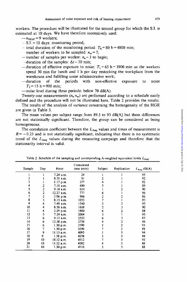
workers. The procedure will be illustrated for the second group for which the S.I. isestimated at 10 days. We have therefore successively used:

— " H G E = 9 workers;—S.I. = 10 days: monitoring period;—total duration of the monitoring period: To = 80 h = 4800 min;—number of workers to be sampled: nw = 7;—number of samples per worker: n, = 3 to begin;—duration of the samples: At = 30 min;—duration of effective exposure to noise: T{ = 65 h = 3900 min as the workers

spend 30 min for lunch and 1 h per day restocking the workplace from thewarehouse and fulfilling some administrative work;

—duration of the periods with non-effective exposure to noiseT2=l5 h = 900min;

—noise level during these periods: below 70 dB(A).Twenty-one measurements («snw) a r e performed according to a schedule easily

defined and the procedure will not be illustrated here. Table 2 provides the results.The results of the analysis of variance concerning the homogeneity of the HGE

are given in Table 3.The mean values per subject range from 89.3 to 93 dB(A) but these differences

are not statistically significant. Therefore, the group can be considered as beinghomogeneous.

The correlation coefficient between the L^cq values and times of measurement isR= —0.23 and is not statistically significant, indicating that there is no systematictrend of the Z-Aeq values during the measuring campaign and therefore that thestationarity interval is valid.

Table 2. Schedule of the sampling and corresponding A-weighted equivalent levels

CumulatedSample Day Hour time (min) Subject

1 1 7.24 a.m. 24 12 1 8.31 a.m. 91 23 1 1.17 p.m. 377 44 2 7.10 a.m. 490 55 2 9.14 a.m. 614 16 2 12.27 a.m. 777 67 2 2.06 p.m. 906 28 3 8.15 a.m. 1055 79 4 7.40 a.m. 1540 5

10 4 8.58 a.m. 1618 211 4 2.29 p.m. 1889 612 5 7.24 a.m. 2004 313 6 9.12 a.m. 2532 614 6 12.38 p.m. 2738 415 6 1.30 p.m. 2790 316 7 1.50 p.m. 3290 717 9 11.13 a.m. 4093 118 9 1.58 p.m. 4258 319 10 10.12 a.m. 4512 720 10 11.22 a.m. 4582 421 10 1.30 p.m. 4710 5

i cation

111121212321322233333

iAeq dB(A)

959292899096869595908895879493899489938888

by guest on July 15, 2011annhyg.oxfordjournals.org

Dow

nloaded from

480 J. Malchaire and A. Piette

Table 3. Analysis of variance of the Z-Acq( levels for the differences between workers

DegreesSource of variation Sum of square of freedom Mean square F test Probability

Between subjects 30.7 6 5.1 0.43 0.85Within subjects 166.0 14 11.9Total 196.7 20

The overall L A e q T level computed according to the equal energy principle for the21 values is equal to 92.3 dB(A), while the arithmetic mean and standard deviationare 91.3 and 3.1 dB(A). The corrected standard deviation computed from the LAeq_r

and mean values according to the Bernard and Castel (1987) expression is equal to3.0 dB(A), the distribution presenting a slight negative skewness (skewnesscoefficient: -0.072).

The daily exposure level is then:

^Ex,d = 92.3 + 10 l o g ^ = 91.4 dB(A)

From the standard deviation 5 = 3.0 dB(A) for 30 min samples, the standarddeviation for 8-h samples can be derived:

O \ 0 3 1

and the standard error can be estimated equal to:

e = 0.3dB(A).

For 21 values, the t value at the 95% level of confidence is equal to 2.086 andtherefore the 95% confidence interval of LEX,d is 91.4±0.6 dB(A). This precision islargely sufficient and no further measurements are needed.

The risks of hearing handicap and disability are respectively estimated at 28%and 11% at age 60 years after 40 years of exposure to that LEX,d-

APPENDIX B: BACKGROUND STUDY

Introduction

The strategy described in the paper uses concepts and formulas presented andvalidated in the literature. However, it appeared necessary to verify whether somehypotheses, and in particular the Larsen (1971) model, defined in the field ofenvironmental pollution, are also valid in the context of noise exposure assessment.A database was built in order to test these hypotheses.

Material and methods

Twenty-two workers performing different tasks in different companies weresurveyed for 8 h per day during 10 consecutive days of work. These includedmechanics, bricklayers and operators for different machines from several sectors of asteel industry and from a manufacture of metallic parts. All were characterized by

by guest on July 15, 2011annhyg.oxfordjournals.org

Dow

nloaded from

Assessment of noise exposure and risk of hearing impairment 481

110

100-

0 1 2 3 4 5 6 7 8Tlme(ti)

Fig. 2. Example of an 8-h recording of the 1 mm equivalent levels.

fluctuating conditions of noise as typically illustrated in Fig. 2, with some periodsspent in less noisy areas (such as control rooms or cafeteria).

A Larson Davis LD705 exposimeter was used, recording the equivalent levelevery minute. From a task analysis, phases with non-effective exposure to noise wereexcluded a priori, leaving a database of a total of 68 713 min of recording.

For each worker, sampling strategies were simulated, as explained above, with—the number of samples ns varying from 3 to 20;—the duration of sampling At varying from 5 to 180 min.The ns samples were taken at random during the period of effective exposure to

noise (duration Tt) for each worker.The procedure was repeated 5000 times in each case and for each subject and a

list of 5000 LAeq?7- was obtained. The variance of these 5000 values (if) wascomputed. Figure 3 illustrates, for two of the 22 workers, how this variance varies asa function of nt and At.

For the whole group of subjects, a covanance analysis was performed with\ogis2) as dependent variable, the number of the subject as independent variable andlog(«,) and log(A0 as covariates.

Results

This analysis of covariance provided the following expression

•> . . . 1

where W-, is a factor depending on the worker and his working condition.

by guest on July 15, 2011annhyg.oxfordjournals.org

Dow

nloaded from

482 J. Malchaire and A. Piette

1 * -

12-

10-

• -

S

4-

,_

0-

•3 mis\ i

\ 5 1

\ 7 1\ \\ i o\V U\\ 15\ »

> 2 0

\ 3 TTTIIB

i 5 \

\ 7 \\ ' \\ 10 1\ u

\ 1 5 17X 20

1\\

\\

\V\\\\\

\

111\\\111\\\

\

\\

\

1\

\1111\11111\\\\

\ \\ \

\

111111\111\\\\\

, \\ V\ \

\

111111\\1\\\

\ \\ V

V

111111\\[\\

\ \

—

\\\

LigendeWORKFR 1

- WORKER 21

\II\ \\ \\ \

10 15 30 120 1 U

AT (mm)Fig. 3. Variance of the distribution of LAo<, levels as a function of the number of samples n, and the

sampling duration A/.

The overall multiple correlation coefficient was 0.974 and both exponents weresignificant at P< 0.001.

This indicates, as used in the strategy, that the accuracy varies roughly inverselyproportionally to the number of samples and the square root of the sampleduration. From this expression, it follows that:

= w,I

and therefore062

This formula is proposed instead of the one presented by Larsen (1971) to derivethe standard deviation for a sampling duration A/2 from the standard deviation foranother sampling duration.

s&T hereabove is the standard deviation of the LAa)T values obtained throughthe 5000 simulations on the database of each subject. In practice, only one campaignof nwn, samples of duration At will of course be conducted. Therefore the onlyestimate of sA, is the standard deviation of the n^n, LAcq values.

A second procedure proposed in the interpretation of the data needed validation:the computation of the standard deviation from the energetic and arithmetic means(LAeq>7- and m) of the distribution of LAaq/ values.

by guest on July 15, 2011annhyg.oxfordjournals.org

Dow

nloaded from

Assessment of noise exposure and risk of hearing impairment

Table 4. A-weighted equivalent level (Z-Aeq); mean (m) and standarddeviation (J) of the 1 min levels; equivalent level (L'ACH derived from m and s;

corrected standard deviation (jcor) and skewness coefficient (s±) for thenoise recordings on 22 subjects in various exposure conditions

483

n

1111034

1819226

161352

1589

147

20121721

w89.089.688.988.988.888.491.491.787.789.091.287.688.188.688.788.190.587.292.389.789.393.4

m

85.787.085.986.285.886.889.489.284.187.688.083.085.185.884.183.385.882.489.487.386.288.9

s

5.85.15.64.95.33.84.34.65.63.45.25.84.94.76.26.16.15.44.54.04.14.3

i-Aeq.T

89.689.989.589.089.188.591.691.787.788.991.186.887.888.488.687.790.085.791.789.288.291.0

•SCOT

5.44.85.24.85.03.74.14.75.63.45.26.35.24.96.36.56.36.55.04.55.26.3

-0.78-0 .60-0.57-0.54-0.41-0.38-0.29-0.29-0.04

0.000.060.070.090.120.180.280.300.510 560.560.721.36

60tndB(A)

Fig. 4. Histogram (1), fitted normal distribution (2) and adjusted normal distribuUon (3) in the case of adistribution of /.Aeq level with negative skewness (worker no. 1).

by guest on July 15, 2011annhyg.oxfordjournals.org

Dow

nloaded from

484 J. Malchaire and A. Piette

1O-

14-

13-

12-

1 1 -

* 10-

s •-is 7"u e-

3 -

2 -

1-

0-

/ \I

/ 2/ / \

/

1 ' \ \/ \ \

/ \ \

I r. \ \• ' - \ \

v-.\• \

/' \ V\•' ' 1 \ x'''.

/ ' / / \ \ \'' 1 I \ ^ '

.• rV ,—=^ ^

L^gende1 * hist2:i

1 ^ 170 80

LA-, in dB(A)100 110 120

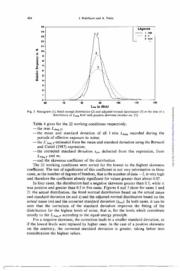
Fig. 5 Histogram (I), fitted normal distribution (2) and adjusted normal distribution (3) in the case of adistribution of LAn) level with positive skewness (worker no. 21).

Table 4 gives for the 22 working conditions respectively:—the true LAeqy,— the mean and standard deviation of all 1 min LAeq recorded during the

periods of effective exposure to noise;—the L'Aeq.r estimated from the mean and standard deviation using the Bernard

and Castel (1987) expression;—the corrected standard deviation scor deducted from this expression, from

^Aeq.r a n d m;

—and the skewness coefficient of the distribution.The 22 working conditions were sorted for the lowest to the highest skewness

coefficient. The test of significance of this coefficient is not very informative in thesecases, as the number of degrees of freedom, that is the number of data —2, is very highand therefore the coefficient already significant for values greater than about 0.07.

In four cases, the distribution had a negative skewness greater than 0.5, while itwas positive and greater than 0.5 in five cases. Figures 4 and 5 show for cases 1 and21 the actual distribution, the fitted normal distribution based on the actual meanand standard deviation (m and s) and the adjusted normal distribution based on theactual mean (m) and the corrected standard deviation (Scor)- In both cases, it can beseen that the correction of the standard deviation improves the fitting of thedistribution for the highest levels of noise, that is, for the levels which contributemostly to the LAeq7- according to the equal energy principle.

For a negative skewness, the correction leads to a smaller standard deviation, asif the lowest levels were replaced by higher ones. In the case of a positive skewnesson the contrary, the corrected standard deviation is greater, taking better intoconsideration the highest values.

by guest on July 15, 2011annhyg.oxfordjournals.org

Dow

nloaded from