A Comparison of Pair Versus Solo Programming Under Different Objectives: An Analytical Approach
23
Information Systems Research Vol. 19, No. 1, March 2008, pp. 71–92 issn 1047-7047 eissn 1526-5536 08 1901 0071 inf orms ® doi 10.1287/isre.1070.0147 © 2008 INFORMS A Comparison of Pair Versus Solo Programming Under Different Objectives: An Analytical Approach Milind Dawande School of Management and the School of Computer Science, University of Texas at Dallas, Richardson, Texas 75083, [email protected] Monica Johar The Belk College of Business, University of North Carolina at Charlotte, Charlotte, North Carolina 28223, [email protected] Subodha Kumar Michael G. Foster School of Business, University of Washington, Seattle, Washington 98195, [email protected] Vijay S. Mookerjee School of Management, University of Texas at Dallas, Richardson, Texas 75083, [email protected] T his study compares the performances of pair development (an approach in which a pair of developers jointly work on the same piece of code), solo development, and mixed development under two separate objectives: effort minimization and time minimization. To this end, we develop analytical models to optimize module-developer assignments in each of these approaches. These models are shown to be strongly NP-hard and solved using a genetic algorithm. The solo and pair development approaches are compared for a variety of problem instances to highlight project characteristics that favor one of the two practices. We also propose a simple criterion that can reliably recommend the appropriate approach for a given problem instance. Typically, for efficient knowledge sharing between developers or for highly connected systems, the pair programming approach is preferable. Also, the pair approach is better at leveraging expertise by pairing experts with less skilled partners. Solo programming is usually desirable if the system is large or the effort needed either to form a pair or to code efficiently in pairs is high. Solo programming is also appropriate for projects with a tight deadline, whereas the reverse is true for projects with a lenient deadline. The mixed approach (i.e., an approach where both the solo and pair practices are used in the same project) is only indicated when the system consists of groups of modules that are sufficiently different from one another. Key words : extreme programming; software development methodology; pair programming; integer programming; genetic algorithms; heuristics History : Paulo Goes, Senior Editor; Giri Kumar Tayi, Associate Editor. This paper was received on April 7, 2006, and was with the authors 8 months for 2 revisions. 1. Introduction The widespread adoption of information technology over the last few decades has created new chal- lenges of delivering information system solutions under ever-tightening deadlines. Development pro- cesses, however, remain challenging and labor inten- sive and hence, new development practices continue to be proposed. These new practices are usually dif- ficult to evaluate; thus claims made by the propo- nents of new approaches often go untested. This is partly because software, being largely intangi- ble, resists quantitative analysis and measurement. Another reason that retards analytic study is the per- ception among software professionals that because software development is a creative process, it should not be organized and managed. 1.1. Problem and Motivation In 1995, Kent Beck, Ward Cunningham, and Ron Jefferies began to explore the extremes of certain soft- ware development practices in an attempt to keep code clean and simple, and ensure flexibility when confronted with changing requirements (Astels et al. 2002). They proposed a novel software development 71
Transcript of A Comparison of Pair Versus Solo Programming Under Different Objectives: An Analytical Approach
Information Systems ResearchVol. 19, No. 1, March 2008, pp. 71–92issn 1047-7047 �eissn 1526-5536 �08 �1901 �0071
informs ®
doi 10.1287/isre.1070.0147©2008 INFORMS
A Comparison of Pair Versus Solo ProgrammingUnder Different Objectives: An Analytical Approach
Milind DawandeSchool of Management and the School of Computer Science, University of Texas at Dallas,
Richardson, Texas 75083, [email protected]
Monica JoharThe Belk College of Business, University of North Carolina at Charlotte,
Charlotte, North Carolina 28223, [email protected]
Subodha KumarMichael G. Foster School of Business, University of Washington, Seattle, Washington 98195,
Vijay S. MookerjeeSchool of Management, University of Texas at Dallas, Richardson, Texas 75083, [email protected]
This study compares the performances of pair development (an approach in which a pair of developersjointly work on the same piece of code), solo development, and mixed development under two separate
objectives: effort minimization and time minimization. To this end, we develop analytical models to optimizemodule-developer assignments in each of these approaches. These models are shown to be strongly NP-hardand solved using a genetic algorithm. The solo and pair development approaches are compared for a varietyof problem instances to highlight project characteristics that favor one of the two practices. We also propose asimple criterion that can reliably recommend the appropriate approach for a given problem instance. Typically,for efficient knowledge sharing between developers or for highly connected systems, the pair programmingapproach is preferable. Also, the pair approach is better at leveraging expertise by pairing experts with lessskilled partners. Solo programming is usually desirable if the system is large or the effort needed either to forma pair or to code efficiently in pairs is high. Solo programming is also appropriate for projects with a tightdeadline, whereas the reverse is true for projects with a lenient deadline. The mixed approach (i.e., an approachwhere both the solo and pair practices are used in the same project) is only indicated when the system consistsof groups of modules that are sufficiently different from one another.
Key words : extreme programming; software development methodology; pair programming; integerprogramming; genetic algorithms; heuristics
History : Paulo Goes, Senior Editor; Giri Kumar Tayi, Associate Editor. This paper was received on April 7,2006, and was with the authors 8 months for 2 revisions.
1. IntroductionThe widespread adoption of information technologyover the last few decades has created new chal-lenges of delivering information system solutionsunder ever-tightening deadlines. Development pro-cesses, however, remain challenging and labor inten-sive and hence, new development practices continueto be proposed. These new practices are usually dif-ficult to evaluate; thus claims made by the propo-nents of new approaches often go untested. Thisis partly because software, being largely intangi-ble, resists quantitative analysis and measurement.
Another reason that retards analytic study is the per-ception among software professionals that becausesoftware development is a creative process, it shouldnot be organized and managed.
1.1. Problem and MotivationIn 1995, Kent Beck, Ward Cunningham, and RonJefferies began to explore the extremes of certain soft-ware development practices in an attempt to keepcode clean and simple, and ensure flexibility whenconfronted with changing requirements (Astels et al.2002). They proposed a novel software development
71

Dawande et al.: Comparison of Pair Versus Solo Programming Under Different Objectives72 Information Systems Research 19(1), pp. 71–92, © 2008 INFORMS
approach, termed extreme programming (XP), wheretwo developers simultaneously work on the samepiece of code (e.g., a module, function, unit, etc.) (Beck2000). Typically, one member of the pair (called thedriver) actually writes the code, while the other (calledthe navigator) observes the creation of the code, sug-gests improvements in structure, points out tacticaland strategic defects, etc. (Williams and Kessler 2003).It has been argued that although pair programmingmay increase the effort to develop a piece of codeas compared to solo programming, this extra effort isoften compensated by lower system integration andtesting effort. Several studies have reported that pairprogramming may lower the integration and testingeffort by 40% to 60% (Erdogmus and Williams 2003,Kuppuswami et al. 2003), but a more conservativefigure of 15% has also been reported (Williams andKessler 2003). Our model draws from several experi-mental studies to derive an expression for the reduc-tion in system integration effort resulting from the useof pair programming. The key trade-off in our modelis between the extra effort needed in pair program-ming to develop modules and the lower effort neededto integrate these modules to create a working system.In addition to pair programming, XP has several
other recommendations, including pair splitting, testplanning before coding, and continuous integration(Beck 2000). Pair splitting ensures that knowledgeabout the system is disseminated among the develop-ers. By pairing with many different partners, devel-opers learn more about the system’s architecture, andshare programming skills (style, tools, techniques,etc.) with other developers. Test data is written evenbefore coding is begun and the system is tested andintegrated almost continuously. Finally, each teammember is allowed to make changes to any part ofthe system.An XP project also entails continuous and intense
user involvement. Users pick valuable system features(called user stories) that describe a path through thesystem (Astels et al. 2002). A user story serves thesame purpose as a use case in traditional softwaredevelopment (Wells 2003). During an iteration, a setof stories is chosen for development. An iteration canrun for as long as six weeks, but a recent surveyshowed that two weeks and three weeks are the mostpopular durations (Beck and Fowler 2001). Iterations
occur in a sequence that depends on several factorsincluding the functionality delivered by the iteration,and the cost and speed of development. Within aniteration, user stories are further broken down intospecific programming tasks (referred to here as mod-ules) and pairs of developers are then assigned tothese tasks (Wells 2003).As is clear from the above discussion, there aremany
aspects embedded in the overall XP methodology. Notall aspects, however, are found in every XP project.In this paper, our analysis focuses on two of the moststriking features, namely, pair programming and pairsplitting. In practice, the task of assigning modules todeveloper pairs is typically done without careful anal-ysis (Williams and Kessler 2003). However, one mustaddress this issue if the numerous benefits of pair pro-gramming and pair splitting are to be realized.
1.2. Objective and ContributionsThis study compares the performances (based oneffort and time) of pair and solo programming.Because the performance of an approach is affectedby the quality of module-developer assignments, anystatement about the relative performance of the twoapproaches must be made for a set of good qualityassignments. This limits the use of empirical data,at least until the pair programming practice maturesand the knowledge of this approach better assimi-lates in the software industry. To further complicatematters, the use of an empirical approach to com-pare performance hinges on the ability to obtain dataon similar projects developed using the pair and soloapproaches.Given these limitations, we follow an analytical
approach to gain insights on the performance of thepair approach relative to the solo approach. Twomathematical models are developed to find optimalmodule-developer assignments for pair and solo pro-gramming. The goal in the effort minimization modelis to minimize the total effort (measured in person-weeks) needed to develop a system on or beforea specified deadline, whereas the goal in the timeminimization model is to minimize the time neededto develop a system while respecting an effort con-straint. For both objectives, it is extremely difficult tosolve realistic problem instances to optimality usingstate-of-the-art solvers (such as CPLEX). Hence, we
Dawande et al.: Comparison of Pair Versus Solo Programming Under Different ObjectivesInformation Systems Research 19(1), pp. 71–92, © 2008 INFORMS 73
propose a heuristic technique—based on a geneticalgorithm (GA)—to solve the problem.For the effort minimization model, without the
deadline constraint, the objective function can be min-imized by assigning a single pair of developers (or asingle developer for solo programming) to all devel-opment tasks. This way, the assigned pair (devel-oper) acquires maximum knowledge of the systemand the integration effort is the lowest possible. How-ever, a single pair (developer) also takes a long time tocomplete the work; thus, in the interest of the deadline,the different development tasks must be done in par-allel by multiple pairs (developers). For the time min-imization model, the presence of an effort constraintrestricts the number of pairs (developers) that canbe used, making the task of producing good qualitymodule-developer assignments quite challenging. Wenext summarize the main contributions of this work.We propose a simple criterion that allows us to pre-
dict whether a particular project can be completedwithless effort using pair programming, or whether the tra-ditional practice of solo programming should be pre-ferred. This criterion is derived using a homogeneoussystem approximation—a simplified approximationof the system where detailed system parameters (e.g.,the effort to develop individual modules, number ofconnections a module has with other modules, etc.)are replaced by a single mean value that appliesto the whole system. The homogeneous approxima-tion is also used to investigate whether the practiceof mixing development regimes for the same projectcan lower development effort over one of the pureapproaches (solo or pair).To extend our analytical results with numerical sim-
ulations, we develop a GA that is shown to provideoptimal or near-optimal solutions for modest-sizedproblems. For problems where a comparison with theoptimal solution cannot be made, the gap between alower bound on the optimal solution and the solu-tion provided by the GA is shown to be reasonablysmall. The GA is therefore used to solve many real-istic problems that are generated based on a realsystem being developed using pair programming ata telecommunications software company. An exper-iment is conducted to investigate the factors thatexplain performance differences between the pair andsolo development methods. The two development
regimes are compared with one another under twodifferent objective criteria: effort and time. Typically,when knowledge sharing between developers is effi-cient or when the system is highly connected (withmany modules that are functionally interdependent),the pair programming practice is preferable. On theother hand, the solo programming practice is usuallydesirable if the effort needed either to form a pairor to code efficiently as a pair is high. The solo pro-gramming practice also emerges more appropriate forprojects with a tight deadline, while the reverse is truewhen the deadline is sufficiently lenient.
1.3. Literature ReviewWe examine several important principles of XP: pairprogramming, knowledge sharing, user involvement,and testing and debugging. One of the most novel fea-tures of XP is pair programming. The claimed ben-efits of pair programming are: better code quality,shorter cycle time, happier developers, better trust andteamwork, more knowledge transfer, and enhancedlearning. (Ambler 2002, Astels et al. 2002, Williamsand Kessler 2003). Some of these benefits have beenexperimentally verified: reduced total effort (Williamsand Kessler 2003), fewer unit and integration errors(Cockburn and Williams 2000, Williams et al. 2000),and simpler code (Wood and Kleb 2002). XP also rec-ommends pair splitting—a practice in which develop-ers change partners during the project. Pair splittingreduces the training time to assimilate new mem-bers, distributes the training burden across the team(Shukla 2002, Williams and Kessler 2003), and main-tains productivity in an environment with high per-sonnel turnover (Benedicenti and Paranjape 2001).Better knowledge sharing among developers is
a key benefit of pair programming (Williams andKessler 2003). Pairing developers allows them to shareknowledge and form a common understanding of thesystem and the development tasks. Sharing occurs inseveral areas such as the client’s evolving require-ments and business environment, new hardware,development tools and languages, and evolving tech-nologies (Curtis et al. 1988, Waltz et al. 1993). Shar-ing of knowledge, however, does not only take placeby being taught or instructed, but also by becoming apractitioner (Brown and Duguid 1991). This tacit orimplicit notion of knowledge sharing is at the heart of
Dawande et al.: Comparison of Pair Versus Solo Programming Under Different Objectives74 Information Systems Research 19(1), pp. 71–92, © 2008 INFORMS
pair programming. More explicit knowledge sharingmethods, however, also contribute to knowledge shar-ing. Dingsoyr (2002) finds that the use of knowledgemanagement tools benefits software quality, reducesdevelopment costs, and improves developer morale.Closely tied to facilitating knowledge sharing in a
software project is the need to coordinate the effortsof the members of a development team. One way tofacilitate coordination is to reduce the cost of mov-ing information between developers. Cockburn andHighsmith (2001) state that in XP such cost reduc-tion is achieved by placing people physically closerto one another, replacing documents with face-to-face discussions, and by improving the team’s amityso that members are more inclined to relay valu-able information quickly. Meixell et al. (2006) applya coordination-theoretic perspective to determine thenumber of developers and the number of sub-tasksinto which any given task of a project should bedivided.Coordination is not only needed among developers,
but also between developers and end users. Involv-ing end users in the development process increasesthe likelihood that requirements are correctly derived,leading to more useful and usable systems (Baeckeret al. 1995, Nielsen 1993). Although several methodsfor deriving software requirements have been pro-posed (Ippolito and Murman 2001), all these meth-ods must contend with requirements that frequentlychange during development (Grunbacher and Hofer2003). Agile software development methods, suchas XP, through continuous end user involvement, areclaimed to better deal with evolving requirements(Beck 2000).Finally, we discuss system testing and integration
practices within XP. This task involves ensuring thatthe components of a software system interact with-out error. Pressman (1992) observes that, irrespectiveof the specific development model followed, systemtesting and integration is required for successfullyexecuting any project. The increasing complexity ofsoftware products, together with shortened develop-ment cycles and higher customer expectations of qual-ity, has elevated the role of software integration andtesting (Hailpern and Santhanam 2002). System inte-gration and testing can be done in a planned oran ad hoc manner. Traditionally, system testing and
integration is often planned or controlled (Pressman1992). XP, on the other hand, proposes continuous andad hoc integration, i.e., the system is fully integratedat all times and XP teams typically “build” the sys-tem several times each day on an “as needed” basis.A claimed benefit of such fine-grained integration andtesting is that it allows easy backtracking and defectisolation (Beck 2000).The rest of this paper is organized as follows.
Section 2 presents the effort minimization and thetime minimization models together with a GAdevised to solve these models. In §3, we derive a cri-terion that can help choose between the pair and soloapproaches on the basis of development effort. Wealso estimate regression models that provide a pre-liminary understanding of the factors that affect therelative performance of the pair and solo approaches.Section 4 details a series of controlled experimentsconducted to closely examine the impact of thesefactors on the performances of the pair and soloapproaches. Section 5 discusses the implications, limi-tations, and possible extensions of the study, and con-cludes the paper.
2. Model and Heuristic SolutionIn this section, we present optimization models forthe effort minimization problem and the time mini-mization problem. At the end of this section, we pro-pose a GA to solve these optimization models. Giventhat pair programming is relatively new, we contactedseveral well-known XP practitioners1 to improve ourunderstanding of how pair programming occurs inpractice.
2.1. PreliminariesFor both the effort minimization and time minimiza-tion problems, we present three versions of the model:solo, pair, and mixed. We use the term module to referto a unit of work assigned to a developer or a pair of
1 Private Communications: E. Herman, Product Sight Corporation,Bellevue, WA.; R.C. Martin, CEO, President and Founder of ObjectMentor Inc., Gurnee, IL.; C. Poole, Founder and Principal of PooleConsulting, Poulsbo, WA.; B. Ramsdell, Co-founder, Brute SquadLabs., acquired by Sendmail, Inc., Emeryville, CA.; R. Rangan, CTOof Product Sight Corporation, Bellevue, WA.; A. Ridlehoover, SBIGroup, Bellevue, WA. S. Sidhartha, Microsoft Corporation, Red-mond, WA.
Dawande et al.: Comparison of Pair Versus Solo Programming Under Different ObjectivesInformation Systems Research 19(1), pp. 71–92, © 2008 INFORMS 75
developers. The solo model requires that each mod-ule be assigned to a single developer; a developer canbe assigned to more than one module. The pair ver-sion requires that each module be assigned to a pair ofdevelopers; the same pair can, of course, work on mul-tiple modules. In the mixed model, a module can beassigned to a single developer or a pair of developers.We consider a system that consists of m mod-
ules that are divided into G groups. In keeping withcommon XP practice, a group of modules corre-sponds to some functionality that must be developedand delivered to users before development work onthe next group is begun. Thus we require that thegroups be developed sequentially, although the mod-ules within a group can be developed in any conve-nient sequence. In each version of the model, the totalsystem development effort (measured in person-weeks)is the sum of the system module development effort, thesystem pair formation effort (equals zero for solo), andthe system integration effort.
2.1.1. Module Development Effort. The moduledevelopment effort is the effort needed to developall the modules in the system. For all three regimes(i.e., solo, pair, and mixed), the module developmenteffort depends on the characteristics of the developers(such as expert, average, or novice) involved. The mod-ule development effort for any given module dependson whether it is developed by a single developer or apair of developers. This effort is typically higher forthe pair approach (relative to solo development) andhas been attributed to the additional effort needed tocommunicate between the members of a pair (Beck2000). This higher effort may be partially diminishedby the additional documentation effort that oftenaccompanies the solo approach to ensure formal com-munication within the team. However, a net higherdevelopment effort associated with pair development(referred to here as the pair development overhead)has been consistently observed in experimental stud-ies (Williams et al. 2000, Nosek 1998, Nawrocki andWojciechowski 2001, Lui and Chan 2004). The pairdevelopment overhead has several positive effects:increased knowledge sharing (Beck 2000), superiortesting and quality of code (Succi et al. 2001), andbetter compatibility of the code with the rest of thesystem (Highsmith and Cockburn 2001). Thus while
pair development requires additional module devel-opment effort, its use could reduce the system inte-gration effort and hence, the total system developmenteffort.
2.1.2. Pair Formation Effort. The second compo-nent of the total system development effort is the sys-tem pair formation effort. Clearly this component iszero for solo programming. The system pair formationeffort is the sum of the pair formation efforts incurredeach time a unique pair is formed. The pair formationeffort is a one-time effort incurred by a pair of devel-opers to establish the mutual understanding neededto work effectively as a team. During pair formation,developers learn to give and accept objective sugges-tions, and to communicate during development. Fora pair, this effort could change with the characteris-tics of the developers (such as expert, average, or novice)involved in the pair (Williams and Kessler 2003).
2.1.3. System Integration Effort. The third com-ponent of the total system development effort is thesystem integration effort. This effort is calculated asthe sum of the efforts needed to integrate each pair offunctionally dependent modules (or links) in the sys-tem. To calculate the system integration effort, we useresults from pair programming experiments that havenoted several important observations: (1) Pair pro-gramming typically lowers system integration effort(Erdogmus and Williams 2003); (2) this reduction isfound to increase with the extent to which pair pro-gramming is used in the project (Kuppuswami et al.2003); and (3) the total reduction from knowledgesharing in pair programming is found to be directlyrelated to the complexity of the integration tasks(Cockburn and Williams 2000). The above findingslead to an expression for system integration effort asdiscussed below.Rather than directly propose an expression for the
system integration effort for a project as a whole, wearrive at an expression for this effort in a constructivemanner by first developing an expression at the linklevel. Let �s
iz be the effort needed to integrate mod-ules i and z using the solo approach when no commondevelopers are used in the development of these mod-ules. Similarly, �p
iz denotes the corresponding effortwhen both modules are developed using the pairapproach, and ��
iz denotes the integration effort when
Dawande et al.: Comparison of Pair Versus Solo Programming Under Different Objectives76 Information Systems Research 19(1), pp. 71–92, © 2008 INFORMS
one module is developed using the solo approach andthe other using the pair approach.Let Cizj = 1 if developer j is common to modules i
and z; 0 otherwise. The total reduction in integra-tion effort (Riz) should be directly proportional to thenumber and characteristics of the developers that arecommon (based on (2) above) and the no-common-developer integration effort (based on (3) above). Thistotal reduction can be expressed as the sum of thereductions due to each common developer; the reduc-tion due to a particular common developer j is Rizj =�j�
kiz, where k = s, p, or �, depending on whether
modules i and z are developed using the solo, pair,or mixed approach, respectively. Here �j (referred tohere as the knowledge sharing coefficient for developer j)is a proportionality constant that captures the impactof developer j being common to the development ofthe two modules. The total reduction in integrationeffort for integrating modules i and z is, therefore,Riz =
∑�j�Cizj=1� Rizj = �k
iz
∑j Cizj�j , where k= s, p, or �.
The resulting integration effort for a link is, therefore,�kiz −Riz = �k
iz�1−∑
j Cizj�j�.The value of �j for a given project is influenced by
factors such as the use of knowledge sharing tools in
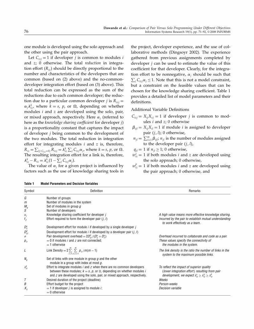
Table 1 Model Parameters and Decision Variables
Symbol Definition Remarks
G Number of groupsm Number of modules in the systemMg Set of modules in group g
S Number of developers�j Knowledge sharing coefficient for developer j A high value means more effective knowledge sharing.fjl Effort required to form the developer pair j� l� Incurred by the pair to establish mutual understanding
to work effectively as a team.Dsij Development effort for module i if developed by a single developer j
Dpijl Development effort for module i if developed by a developer pair (j� l)
� Pair development overhead= 2Dpijl /D
sij +Ds
il � Overhead incurred to collaborate and code as a pair.piz = 0 if modules i and z are not connected; These values specify the connectivity of
= 1 otherwise the modules in the system.
L Link Density= 2m∑i=1
m∑z=i+1
piz/mm− 1� The link density is the ratio the number of links in thesystem to the maximum possible links.
Ng Set of links with one module in group g and the othermodule in a group with index at most g.
�kiz Effort to integrate modules i and z when there are no common developersbetween these modules; k = s, p, or �, depending on whether modules i
and z are developed using the solo, pair, or mixed approach, respectively.
To reflect the impact of superior qualitylower integration effort � resulting from pairdevelopment, we expect �siz ≥ ��iz ≥ �piz
T Desired duration of the project (deadline) WeeksB Effort budget for the project Person-weeksXij = 1 if developer j is assigned to module i; Decision variable
= 0 otherwise
the project, developer experience, and the use of col-laborative methods (Dingsoyr 2002). The experiencegathered from previous assignments completed bydeveloper j can be used to estimate the value of thiscoefficient for that developer. Clearly, for the integra-tion effort to be nonnegative, �j should be such that∑
j Cizj�j ≤ 1. Note that this is not a model constraint,but a constraint on the feasible values that can bechosen for the knowledge sharing coefficient. Table 1provides a detailed list of model parameters and theirdefinitions.
Additional Variable Definitions
Cizj = XijXzj = 1 if developer j is common to mod-ules i and z; 0 otherwise
�ijl = XijXil = 1 if module i is assigned to developerpair �j� l�; 0 otherwise,
njl =∑m
i=1�ijl; njl is the number of modules assignedto the developer pair �j� l�,
qjl = 1 if njl ≥ 1; 0 otherwise,ws
iz = 1 if both modules i and z are developed usingthe solo approach; 0 otherwise,
wpiz = 1 if both modules i and z are developed using
the pair approach; 0 otherwise, and
Dawande et al.: Comparison of Pair Versus Solo Programming Under Different ObjectivesInformation Systems Research 19(1), pp. 71–92, © 2008 INFORMS 77
w�iz = 1 if one of modules i and z is developed using
the solo approach and the other is developedusing the pair approach; 0 otherwise.
2.2. Effort MinimizationThe goal is to select an optimal module-developerassignment scheme such that the total system devel-opment effort is minimized. In addition, it is requiredthat the project be completed on or before a specifieddeadline. The formal model for effort minimization ispresented below.
Minimizem∑i=1
S∑j=1
DsijXij +
m∑i=1
S∑j=1
S∑l=j+1
�ijl�Dp
ijl −Dsij −Ds
il�
+S−1∑j=1
S∑l=j+1
fjlqjl +m−1∑i=1
m∑z=i+1
[�sizw
siz +�
pizw
piz +��
izw�iz
−S∑
j=1�j��
sizw
sizCizj +�
pizw
pizCizj +��
izw�izCizj �
]piz�
Subject to:
Time Constraints∑i∈M1
[Ds
ijXij +∑l �=j
�ijl�0�5Dp
ijl −Dsij �
]+
S∑l=10�5fjlqjl
+ ∑�i−z�∈N1
[�siz
2�ws
izxij +wsizxzj �+
�piz
4�w
pizxij +w
pizxzj �
+ ��iz
3�w�
izxij +w�izxzj �
−S∑
l=1�l
(�siz
2�ws
izxijCizl +wsizxzjCizl�
+ �piz
4�w
pizxijCizl +w
pizxzjCizl�
+ ��iz
3�w�
izxijCizl +w�izxzjCizl�
)]≤ T1
∀ j = 1�2� � � � � ST1+
∑i∈M2
[Ds
ijXij +∑l �=j
�ijl�0�5Dp
ijl −Dsij �
]
+ ∑�i−z�∈N2
[�siz
2�ws
izxij +wsizxzj �+
�piz
4�w
pizxij +w
pizxzj �
+ ��iz
3�w�
izxij +w�izxzj �
−S∑
l=1�l
(�siz
2�ws
izxijCizl +wsizxzjCizl�
+ �piz
4�w
pizxijCizl +w
pizxzjCizl�
+ ��iz
3�w�
izxijCizl +w�izxzjCizl�
)]≤ T2
∀ j = 1�2� � � � � S�Similarly, there are sequential constraints for groups3�4� � � � �G− 1.Finally,
TG−1+∑i∈MG
[Ds
ijXij +∑l �=j
�ijl�0�5Dp
ijl −Dsij �
]
+ ∑�i−z�∈NG
[�siz
2�ws
izxij +wsizxzj �+
�piz
4�w
pizxij +w
pizxzj �
+ ��iz
3�w�
izxij +w�izxzj �
−S∑
l=1�l
(�siz
2�ws
izxijCizl +wsizxzjCizl�
+ �piz
4�w
pizxijCizl +w
pizxzjCizl�
+ ��iz
3�w�
izxijCizl +w�izxzjCizl�
)]≤ T
∀ j = 1�2� � � � � S�Module Assignment Constraints
For Solo ProgrammingS∑
j=1Xij = 1 ∀ i= 1�2� � � � �m�
exactly one developer is assigned to every module.For Pair Programming
S∑j=1
Xij = 2 ∀ i= 1�2� � � � �m�
exactly two developers are assigned to every module.For Mixed Programming
S∑j=1
Xij ≥ 1 ∀ i= 1�2� � � � �m�
all modules must be assigned to at least onedeveloper.
S∑j=1
Xij ≤ 2 ∀ i= 1�2� � � � �m�
at most two developers can be assigned to anymodule.
Dawande et al.: Comparison of Pair Versus Solo Programming Under Different Objectives78 Information Systems Research 19(1), pp. 71–92, © 2008 INFORMS
In the objective function, the term∑m
i=1∑S
j=1DsijXij +∑m
i=1∑S
j=1∑S
l=j+1�ijl�Dp
ijl −Dsij −Ds
il� measures the totalmodule development effort. For a module i, �Dp
ijl −Ds
ij − Dsil� measures the extra development effort
incurred when module i is developed by a pair ofdevelopers. The term
∑mi=1
∑Sj=1D
sijXij represents the
total development effort using solo programming forall the modules, and the term
m∑i=1
S∑j=1
S∑l=j+1
�ijl�Dp
ijl −Dsij −Ds
il�
represents the total pair development overhead formodules that were developed by the pair approach.The second term in the objective function,∑S−1j=1
∑Sl=j+1 fjlqjl, measures the total pair formation
effort. The indicator variable qjl is set to 1 if the num-ber of modules assigned to developer pair �j� l� isat least one. The last term in the objective functionmeasures the integration effort; the justification forthis expression has already been provided earlier.We next discuss the formulation of the project dead-
line constraint. Note that we require that the groupsin the system be completed sequentially. The projectcompletion time constraint enforces that the lastgroup must be completed before (or by) the dead-line T . The completion time of the last group is calcu-lated as the completion time of the last-but-one groupplus the time required for developing and integrat-ing the last group. In general, the completion time ofany group is calculated as the completion time of theprevious group plus the development and integrationtime required for this group. The time required for agroup is the maximum of the values of the time spentby each developer in that group. For any group, ifmodule i is developed by a single developer j , thenthis developer incurs a development time of Ds
ij . If,on the other hand, module i is developed by a pair�j� l�, then developers j and l each incur a develop-ment time of 0�5Dp
ijl. Over all the modules in group g,the total module development time for developer j
is, therefore,∑
i∈MgDs
ijXij +∑
l �=j �ijl�0�5Dp
ijl −Dsij �. Simi-
larly, if a developer pair �j� l� is formed, then develop-ers j and l each incur a pair formation time of 0�5fjl.Hence, the total pair formation time for developer jis
∑Sl=1 0�5fjlqjl. We next consider the integration time
incurred by developer j for the group. The integra-tion effort for any given link (i� z) is proportionately
distributed among the developers (i.e., proportionalto each developer’s involvement in the developmentof modules i and z). For example, suppose module i
was developed by developers A and B, and module zwas developed by developers A and C. Then, devel-oper A incurs half of the effort to integrate link (i� z)while developers B and C each incur a fourth of thiseffort. This integration time is added to developer j’smodule development time and pair formation time(when applicable) to yield the total time spent by thatdeveloper for the group.Before we end the discussion pertaining to the
effort minimization model, note that the above modelwould remain structurally unchanged if the moduledevelopment effort, the link integration effort, andthe pair formation effort were stochastic quantitiesand the expected system development effort was beingoptimized. This is because the objective function andthe set of constraints are linear in Ds
ij , Dp
ijl, fjl, �siz, �
piz,
and ��iz.
2.3. Time MinimizationHere, we minimize the time needed to complete aproject subject to the constraint that the total systemdevelopment effort does not exceed a specified effortbudget. Such a time minimization model may be use-ful to solve from the perspective of a project managerwho is provided with a fixed set of resources, butneeds to optimize project decisions so as to developthe system as quickly as possible. The model formu-lation for this problem is similar to that of the effortminimization problem except for one obvious change:the objective is to minimize the completion time ofthe project and the resource constraint pertains to aneffort budget rather than a time deadline. For details,see Appendix A of the online supplement.2
In the effort and time minimization models, theobjective functions and the constraints have somenonlinear terms (involving 0-1 variables), and hencethese models cannot be directly solved by a linearinteger program solver. However, it is straightforwardto linearize them using standard mathematical pro-gramming techniques (Glover and Woolsey 1974). The
2 An online supplement for this paper is available on the Infor-mation Systems Research website (http://isr.pubs.informs.org/ecompanion.html).
Dawande et al.: Comparison of Pair Versus Solo Programming Under Different ObjectivesInformation Systems Research 19(1), pp. 71–92, © 2008 INFORMS 79
additional variables and constraints required for thelinearized version are provided in Appendix A ofthe online supplement. (See footnote 2.)
2.4. Problem ComplexityThe models developed in the previous section can besolved to provide optimal module-developer assign-ments so that a fair comparison between the pair andsolo approaches can be conducted. A practical ques-tion arises: How easy is it to solve these models? Torespond to such a concern about problem complexity,we first note that these models are, in general, hard tosolve. The pair programming version of the effort min-imization problem is strongly NP-hard and both soloand pair versions of the time minimization problemare also strongly NP-hard. The mathematical proofs ofthe above claims can be found in Appendix A of theonline supplement. (See footnote 2.)Because the problem is strongly NP-hard, for prob-
lems beyond a certain size, finding an optimal solu-tion in a reasonable amount of time can be difficult(Garey and Johnson 1979). We therefore devise aheuristic approach to obtain near-optimal solutionsrelatively quickly. Both the effort and the time mini-mization problems exhibit some structural similarityto the Quadratic Assignment Problem (QAP). In theQAP, facilities need to be assigned to locations undera cost minimizing objective that is naturally nonlinear(quadratic). Similarly, in the effort and the time min-imization problems, the primary decision is to assigndevelopers to modules with the objective of minimiz-ing a nonlinear function. A solution technique basedon a GA has been successfully applied to solve theQAP (Drezner 2003). We therefore exploit this struc-tural similarity to devise a GA to solve our problems.The GA is briefly discussed below.
2.5. Genetic AlgorithmGAs belong to a class of heuristic optimization tech-niques that use randomization as well as directedsearch to find optimal or near-optimal solutions. Thedevelopment of GAs was inspired by evolutionaryprocesses through which life is believed to haveevolved to its present forms. Goldberg (1989) has suc-cessfully applied GAs to solve many different com-binatorial problems. For QAP, solutions based on
GAs have been proposed in several studies includ-ing, Ahuja et al. (2000), Drezner (2003), Fleurent andFerland (1994), and Tate and Smith (1995).For both the effort and the time minimization prob-
lems, we devise a GA that is based on the ideas pro-posed by Drezner (2003). The average performanceof Drezner’s algorithm has been shown to be signifi-cantly better than that of other algorithms available inthe literature. More specifically, for a well-known testset consisting of 29 minimization problems, the valueof the solution from Drezner’s algorithm exceeded thebest-known solution by only 0.037% on the average.Moreover, the algorithm is better by about a factorof 20, both with respect to the quality of the solutionand the run time, than an earlier algorithm proposedby Ahuja et al. (2000).The details of the proposed GA are provided in
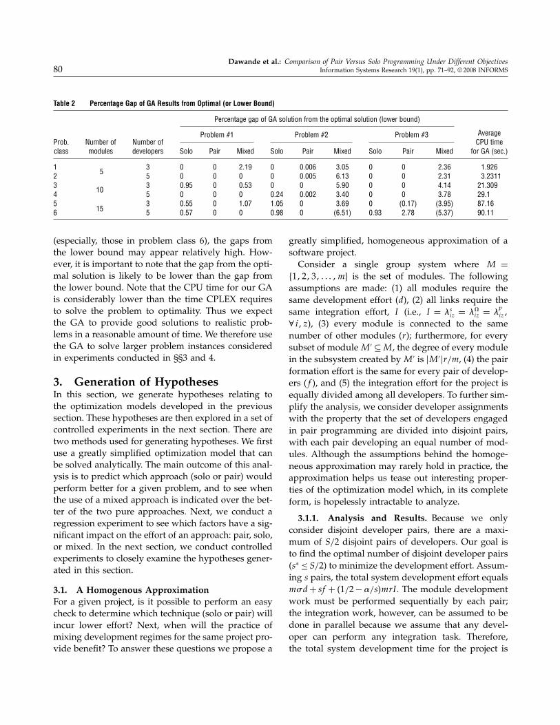
Appendix A of the online supplement. (See foot-note 2.) To measure the performance of the GA, wecompare its solution with either the optimal solution(when it can be found) or a lower bound on the opti-mal solution (when finding an optimal solution in notpracticable). For this comparison, we consider threevalues for the number of modules and two values forthe number of developers. Hence, there are six (3×2)problem classes. For each problem class, we generatethree problem instances by varying the other modelparameters.All experiments were carried out on a Pentium IV
computer (3.0 GHz, 2 GB RAM) with Windows XP asthe operating system. For each problem instance, weused CPLEX (version 8.1.0) to solve the integer pro-gramming formulation of all three approaches (solo,pair, and mixed). We also used the proposed GAto solve these problem instances. The results of thiscomparison are reported in Table 2. CPLEX couldnot solve a few problem instances to optimality, butalways provided a lower bound on the optimal solu-tion. For the cases where CPLEX did not provide anoptimal solution within an imposed time limit of threehours, we compare the solution from the GA with thelower bound; these results are indicated by numbersenclosed in parentheses.From Table 2, it can be seen that our GA provides
optimal or near-optimal solutions for the probleminstances in the test bed. For a few problem instances
Dawande et al.: Comparison of Pair Versus Solo Programming Under Different Objectives80 Information Systems Research 19(1), pp. 71–92, © 2008 INFORMS
Table 2 Percentage Gap of GA Results from Optimal (or Lower Bound)
Percentage gap of GA solution from the optimal solution (lower bound)
Problem #1 Problem #2 Problem #3 AverageProb. Number of Number of CPU timeclass modules developers Solo Pair Mixed Solo Pair Mixed Solo Pair Mixed for GA (sec.)
1 3 0 0 2�19 0 0�006 3�05 0 0 2�36 1�9262 5 0 0 0 0 0�005 6�13 0 0 2�31 3�2311
5
3 3 0�95 0 0�53 0 0 5�90 0 0 4�14 21�3094 5 0 0 0 0�24 0�002 3�40 0 0 3�78 29�1
10
5 3 0�55 0 1�07 1�05 0 3�69 0 0�17� 3�95� 87�166 5 0�57 0 0 0�98 0 6�51� 0�93 2�78 5�37� 90�1115
(especially, those in problem class 6), the gaps fromthe lower bound may appear relatively high. How-ever, it is important to note that the gap from the opti-mal solution is likely to be lower than the gap fromthe lower bound. Note that the CPU time for our GAis considerably lower than the time CPLEX requiresto solve the problem to optimality. Thus we expectthe GA to provide good solutions to realistic prob-lems in a reasonable amount of time. We therefore usethe GA to solve larger problem instances consideredin experiments conducted in §§3 and 4.
3. Generation of HypothesesIn this section, we generate hypotheses relating tothe optimization models developed in the previoussection. These hypotheses are then explored in a set ofcontrolled experiments in the next section. There aretwo methods used for generating hypotheses. We firstuse a greatly simplified optimization model that canbe solved analytically. The main outcome of this anal-ysis is to predict which approach (solo or pair) wouldperform better for a given problem, and to see whenthe use of a mixed approach is indicated over the bet-ter of the two pure approaches. Next, we conduct aregression experiment to see which factors have a sig-nificant impact on the effort of an approach: pair, solo,or mixed. In the next section, we conduct controlledexperiments to closely examine the hypotheses gener-ated in this section.
3.1. A Homogenous ApproximationFor a given project, is it possible to perform an easycheck to determine which technique (solo or pair) willincur lower effort? Next, when will the practice ofmixing development regimes for the same project pro-vide benefit? To answer these questions we propose a
greatly simplified, homogeneous approximation of asoftware project.Consider a single group system where M =
�1�2�3� � � � �m} is the set of modules. The followingassumptions are made: (1) all modules require thesame development effort (d), (2) all links require thesame integration effort, I (i.e., I = �s
iz = ��iz = �
piz�
∀ i� z), (3) every module is connected to the samenumber of other modules (r); furthermore, for everysubset of moduleM ′ ⊆M , the degree of every modulein the subsystem created byM ′ is �M ′�r/m, (4) the pairformation effort is the same for every pair of develop-ers (f ), and (5) the integration effort for the project isequally divided among all developers. To further sim-plify the analysis, we consider developer assignmentswith the property that the set of developers engagedin pair programming are divided into disjoint pairs,with each pair developing an equal number of mod-ules. Although the assumptions behind the homoge-neous approximation may rarely hold in practice, theapproximation helps us tease out interesting proper-ties of the optimization model which, in its completeform, is hopelessly intractable to analyze.
3.1.1. Analysis and Results. Because we onlyconsider disjoint developer pairs, there are a maxi-mum of S/2 disjoint pairs of developers. Our goal isto find the optimal number of disjoint developer pairs(s∗ ≤ S/2) to minimize the development effort. Assum-ing s pairs, the total system development effort equalsm)d+ sf + �1/2−�/s�mrI . The module developmentwork must be performed sequentially by each pair;the integration work, however, can be assumed to bedone in parallel because we assume that any devel-oper can perform any integration task. Therefore,the total system development time for the project is
Dawande et al.: Comparison of Pair Versus Solo Programming Under Different ObjectivesInformation Systems Research 19(1), pp. 71–92, © 2008 INFORMS 81
0�5�f +m)d/s�+mrI�s−2��/4s2. We need to choose sto minimize total effort subject to the deadline con-straint. For the solo approach, the total system devel-opment effort (module development plus integration)is md +mrI�S − ��/2S, and the total time needed ismd/S+mrI�S−��/2S2. We need to choose S to mini-mize total effort subject to the deadline constraint. Itcan be shown that the following effort criterion indi-cates that the pair approach would finish the projectwith less effort than the solo approach (see Appen-dices B and C in the online supplement [footnote 2]):
s∗*2s∗S∗f +m�2)dS∗ − 2dS∗ + r�I�+ < 2mr�IS∗�
The other purpose of the homogeneous approxima-tion is to explore whether the use of a mixed approachis indicated for a given project. Here we obtain anintuitive result: the better of the two pure approaches(solo or pair) matches the performance of the mixedapproach (see Appendix D in the online supplement,[footnote 2]). This result is expected; under homo-geneity, optimal solutions should lie at one of theextremes (solo or pair). However, this result is anartifact of the homogeneous assumption. We there-fore ask: to what extent (of heterogeneity) does the“pure =mixed” result hold? Furthermore, when themixed approach does perform better, how substantialis the improvement? In §4, we will investigate the fol-lowing two main questions that arise from the aboveanalysis:(a) For a given project how accurate is the predic-
tion—based on a homogeneous approximation of thesystem—concerning the relative performance (basedon development effort) of the solo versus the pairapproach?(b) To what extent of heterogeneity does the per-
formance of the better of the two pure approaches(solo and pair) match the performance of the mixedapproach?
3.2. Hypotheses Concerning Solo andPair Development Efforts
We next generate a set of hypotheses that are aimed ata direct comparison—based on development effort—between the solo and pair development approaches.To generate these hypotheses, we have relied on intu-ition to identify some of the more obvious effects. In
addition, we use the results of a regression exper-iment that helps us identify more complex effects.We begin with a discussion of several specific projectfactors that could have a significant impact on the rel-ative performance of the pair and solo programmingapproaches.
3.2.1. Discussion of Factors. The factors clusterinto three categories: (1) system parameters, (2) effortparameters, and (3) project parameters.
System ParametersNumber of Modules (m) is the total number of mod-ules in the system. Each module takes more effort todevelop using pair programming.
Link density (L) is the ratio of the total number oflinks between modules in the system to the maximumnumber of links possible for that system (i.e., wheneach module is connected to all other modules). Asthe number of links in the system increases, the inte-gration effort increases.
Effort ParametersThe Knowledge Sharing Coefficient (�) affects the effortsavings to integrate a link from using common devel-opers to build the modules that form the link.Because pair programming can be expected to dis-seminate system knowledge more effectively, the pairapproach may enjoy a relative advantage over thesolo approach as the knowledge sharing coefficient isincreased.
Pair Effort Factors (f �)) only affect the pair pro-gramming approach. As mentioned earlier, pairformation effort—also referred to as pair jellingeffort—is the initial adjustment effort required to tran-sition from solitary to collaborative programming.Another factor related to pair programming, the pairdevelopment overhead, is the additional effort neededby a pair of developers to develop a module whencompared to the effort incurred by an individualdeveloper to build the same module.
Project ParametersProject Deadline (T ) is the total time available to com-plete the project. As the project deadline tightens,more parallel work must occur to complete the sys-tem within schedule. As more work is performedin parallel, the knowledge dissemination advantage
Dawande et al.: Comparison of Pair Versus Solo Programming Under Different Objectives82 Information Systems Research 19(1), pp. 71–92, © 2008 INFORMS
of pair programming should reduce. Another projectrelated parameter is the number of developers (S) avail-able for the project. For a given project, the num-ber of developers and the project deadline are clearlyrelated: more developers would typically be requiredto complete a given project in less time. Rather thanvarying both the project completion time and theteam size, we keep the team size constant at sevendevelopers and generate project deadlines that aretight or relaxed in relation to this fixed team size.
Team Expertise (ne) is the number of expert devel-opers in the team. This factor influences systemdevelopment effort because it is assumed that expertdevelopers can perform the same task with less effort.The above factors are varied to create realistic project
conditions to explore their effects. Real software sys-tems, however, can vary widely in many aspects suchas structure, scope, complexity, etc., and in a numericalexperiment, all nuances of a real software system aredifficult to capture. To generate the data for our exper-iments we used artificial systems, but anchored thecharacteristics of these systems in some real context—a billing application being implemented using pairprogramming methods at a large telecommunicationssoftware company. The details of the billing systemand the numerical factor values used in the experimentare described in the appendix (see Appendix E in theonline supplement, [footnote 2]).We use the following model,
Effort�E� = B0+B1X+B2�+B3f +B4) +B5m+B6ne
+B7L+B8T + Interaction Terms� (1)
The model has one indicator variable (X = 1 for pair,= 0 for solo), six quantitative variables (��f �)�m�ne,and L), and one ordinal variable (T ), each with twolevels (low and high). The estimated regression modelis presented in Appendix E in the online supplement(see footnote 2). The parameters are estimated usingthe Ordinary Least Squares approximation in SAS9.1. Firstly, a reduced form of the model is obtainedusing stepwise regression. In the reduced model, onlyterms with p-value below 0.05 are considered signif-icant. To eliminate multicollinearity, we use a partialorthogonalization of interaction terms (Burrill 1997,Yu 2000). Using this method we were able to deriveparameter estimates of all explanatory variables with
variation inflation factors less than 6, indicating thatafter orthogonalization, the multicollinearity problemhad been resolved (Kleinbaum et al. 1998, p. 210).For robustness, we also verified that the conditionindices and tolerances associated with the parameterestimates demonstrated the absence of multicollinear-ity among the explanatory variables (see AppendixE in the online supplement [footnote 2]). In addi-tion, a well-known goodness-of-fit test for normality(Kolmogorov-Smirnov) was used to verify that theerror term in (1) is normally distributed with a meanof zero.
3.2.2. Hypotheses. We next present seven state-ments that summarize the impact of the various fac-tors on the effort of the pair and solo approaches.These statements are further examined in a controlledexperiment in §4. The first four statements below listconditions that put the pair approach at a disadvan-tage followed by another three statements that listconditions which favor the use of the pair develop-ment approach. All statements below use total systemdevelopment effort as the basis of comparison.
Hypothesis 1. Increasing the pair development over-head always puts the pair approach at a disadvantage rela-tive to the solo approach.
This hypothesis is easy to motivate: Because increas-ing the pair development overhead only worsensthe performance of the pair approach, this approachshould be put at a relative disadvantage when the pairdevelopment overhead is increased.
Hypothesis 2. The relative disadvantage of increasingthe pair development overhead for the pair approach ismagnified for a system with more modules, and with highvalues for the knowledge sharing coefficient or the projectdeadline.
It is reasonable to expect the relative disadvan-tage to increase with more modules in the systembecause each module requires relatively more effort tobe developed as a pair. The impact of the knowledgesharing coefficient on the relative disadvantage ismore subtle, however. As the pair development over-head is increased, more development effort is neededby the pair approach than by the solo approach.For a fixed project deadline, the only way to accom-plish this additional development effort is for the
Dawande et al.: Comparison of Pair Versus Solo Programming Under Different ObjectivesInformation Systems Research 19(1), pp. 71–92, © 2008 INFORMS 83
pair approach to use more pairs to complete theproject. Hence, knowledge sharing could suffer andthe relative impact of reduced knowledge sharingshould be more at higher values of the knowledgesharing coefficient. Finally, the manner in which theproject deadline affects the relative disadvantage isalso related to the number of pairs used to completethe project. At low values of the project deadline, rel-atively more pairs are already necessary to completethe project and hence increasing the pair developmentoverhead should not have much impact on the num-ber of pairs used. On the other hand, at high val-ues of the project deadline, the pair approach is ableto use relatively fewer pairs and hence benefit fromits superior knowledge sharing ability. This ability isrestricted by increasing the pair development over-head and hence, the relative disadvantage (of increas-ing the pair development overhead) should be feltmore when the value of the project deadline is highrather than low.
Hypothesis 3. Increasing the pair formation effort hasa negative impact on the pair approach relative to the soloapproach only when the project deadline is relatively tight�i.e., a low value of the deadline�.
The forces behind this hypothesis are similar tothe ones discussed above. Since the pair formationeffort applies to each pair being formed, the impactof increasing the pair formation effort should dependon the number of pairs being used to complete theproject. For a project with a tight deadline, it isnecessary to use relatively more pairs to completethe project before the specified deadline. Hence, theimpact should be more for a project with a tightdeadline.
Hypothesis 4. Increasing the number of modules putsthe pair approach at a relative disadvantage when the pairdevelopment overhead is high and the link density is low.
The intuition behind the first part of the abovehypothesis is clear and has been discussed earlier.When the number of modules is increased at highvalues of the link density, the number of links alsoincreases rapidly and this should favor the pairapproach, thus compensating to a certain extent, theincrease in the number of modules. Hence the rela-tive disadvantage should be felt more when the linkdensity is low.
Hypothesis 5. Increasing the knowledge sharing coef-ficient benefits the pair development approach relative tothe solo approach. However, this relative advantage is weak-ened when the pair development overhead is high.
The first statement above is intuitive and resultsfrom the superior knowledge sharing ability of thepair approach. The second statement (concerning therelative advantage being weakened) has been dis-cussed earlier: when the pair development overheadis high, more pairs are necessary to complete theproject and this restricts the advantage of the pairapproach to exploit knowledge sharing. Hence, therelative advantage of increasing the knowledge shar-ing coefficient can be expected to weaken when thepair development overhead is high.
Hypothesis 6. Increasing the link density in a systembenefits the pair development approach relative to the soloapproach. This relative advantage increases as the numberof modules in the system increases.
The first statement is intuitive. As higher values oflink density, the integration effort in the project is rela-tively higher. Generally speaking, the relative strengthof the pair approach has to do with its lower integra-tion effort. Hence, we should expect that increasingthe link density should favor the pair approach. Thesecond statement is also easy to explain. With moremodules in the system, increasing the link density hasa greater impact on the number of links in the system.Hence, the relative advantage should increase.
Hypothesis 7. Relaxing �i.e., increasing� the projectdeadline puts the pair approach at a relative advantage overthe solo approach. This relative advantage increases for highvalues of the pair formation effort and reduces for high val-ues of the pair development overhead.
The first statement can be explained by the fact thatwhen the project deadline is lenient, the pair approachis able to form relatively fewer pairs, and henceexploit its knowledge sharing advantage. The relativeadvantage is magnified at high values of the pair for-mation effort because increasing the project deadlinenot only increases knowledge sharing (by formingfewer pairs) but, more directly, reduces the total pairformation effort. The last effect above concerns thefact that at high values of the pair development over-head, relatively more pairs need to be created to com-plete the project within the specified deadline. Hence,

Dawande et al.: Comparison of Pair Versus Solo Programming Under Different Objectives84 Information Systems Research 19(1), pp. 71–92, © 2008 INFORMS
the relative advantage of the pair approach (resultingfrom superior knowledge sharing) should diminish.
4. Controlled ExperimentsThe empirical and analytical methods used in theprevious section provided us with several hypothe-ses that we explore in depth in this section. Thesehypotheses need further exploration because neitherthe regression model nor the homogeneous approx-imation was sufficiently detailed. The results fromthe homogeneous approximation are questionablebecause of the strong homogeneity assumptions madeto obtain these results. Also, for practical reasons, theregression model used only two levels for each factor.Two level variations do not provide much sense of thenature of the relationship between a particular factorand the outcome variable of interest (effort or time).In these experiments, we isolate a factor of interestand vary it in small increments from a low value to ahigh value. The other factors are held constant whilethe factor of interest is being varied. To permit someinvestigation into factor interactions, an experiment isrepeated for different values of the interacting factorof interest.To begin, we evaluate the predictive ability of the
effort criterion developed in the previous section overa wide range of problems. To summarize, the effortcriterion correctly predicted for about 83.59% of the128 instances to which it was applied. Despite thehomogeneity assumptions, the various influencingfactors appear to “average” out at least as far as theordinal ranking of the pair and solo approaches is con-cerned. Thus, for effort minimization problems, thecriterion should prove to be quite useful to providea rough guideline on when the pair approach shouldbe used.
4.1. Pure Versus MixedAs regards the issue of “pure versus mixed,” we firstuse the data generated for the regression experimentsto test whether mixing development approaches inthe same project can lower the development effort.The one-tailed t-test shows that it is not necessary tomix the solo and the pair development practices in thesame project. We now investigate this result in greaterdetail using the controlled experiments.
The controlled experiments allow us to make twoobservations. The first observation is that the “pure=mixed” result continues to hold as long as the groupsshare the same average characteristics (e.g., the aver-age number of links emanating from given module).Within a group, differences between modules (e.g.,some modules being more connected than others) donot indicate the use of a mixed approach. Thus, “inter-group” variation is more indicative of the use of amixed approach than “intra-group” variation.Our inferences above draw from two separate
experiments. In the first experiment, we let intra-group variation increase, but keep the mean charac-teristics of the groups constant. For example, whenthe connection probability is 0.1, all groups have thecharacteristic that any pair of modules in a groupis connected with a probability of 0.1. The connec-tion “event” between modules is a Bernoulli variablewith a variance of 0�1 ∗ �0�9�. As the connection prob-ability increases from 0.1 to 0.5, it is clear that theintra-group variation should increase. However, thisincrease does not seem to affect the pure versus mixedchoice; a pure approach always matches the perfor-mance of the mixed approach.In the second experiment, we create differences in
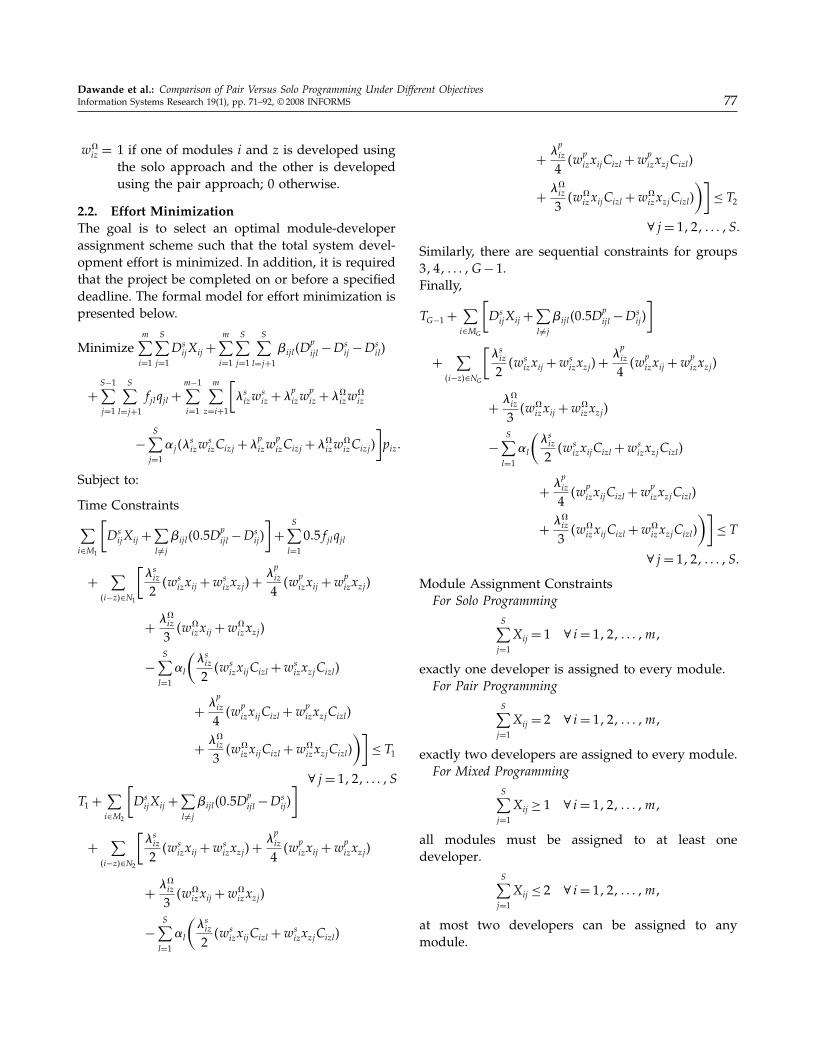
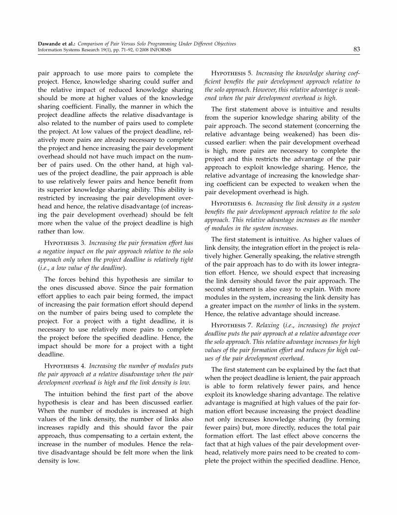
the mean characteristics of the groups; the groups aredifferent in terms of the mean connection probability.In this experiment, the number of links is determinedbased on the connection probability between the mod-ules within a group and the connection probabilitybetween the modules across groups. Because the num-ber of links within a group is usually much higherthan the number of links across any two groups, theconnection probability between the modules acrossgroups is fixed at 0.02 and the connection probabilitybetween the modules in the first group is fixed at 0.95;for the other groups, this probability is varied sys-tematically as shown in Figure 1. The other parametervalues used in the second experiment are as follows:Number of Groups= 3, Number of Modules= 20, PairDevelopment Overhead= 1�25, Project Deadline= 3�4Weeks, Number of Developers= 7, Number of ExpertDevelopers = Number of Novice Developers = 2.Finally, the mean knowledge sharing coefficient wasset at 0.45 and the mean pair formation effortwas chosen to be 0.15 person-weeks; the variationin these parameters was generated as described in
Dawande et al.: Comparison of Pair Versus Solo Programming Under Different ObjectivesInformation Systems Research 19(1), pp. 71–92, © 2008 INFORMS 85
Figure 1 Comparison of Pure Versus Mixed Approaches
0
2
4
6
0.20.40.60.81.0
Connection probability for second and third groups
Perc
enta
ge d
iffe
renc
ebe
twee
n ef
fort
s
Percentage difference frompure effort to mixed effort
Percentage difference frompure-groups effort tomixed effort
Connection probability for first group = 0.95
Table 3 Base Parameter Values for Examining the Factor Effects
Mean knowledge Mean pairG M sharing coefficient formation effort L � S
6 40 0.15 0.30 person-weeks 0.11 1.15 7
Appendix E.2 of the online supplement (see foot-note 2). The results of the second experiment areshown in Figure 1. Note that the percentage differencefrom pure effort to mixed effort is calculated as:
Percentage Difference from Pure Effort
to Mixed Effort= Pure Effort−Mixed EffortPure Effort
× 100�
In Figure 1, the dashed line shows the improvementof the mixed approach over the better of the twopure approaches. Here, the mixed approach is alwaysindicated as the development method of choice. Oursecond observation comes from a closer look at situa-tions when the use of a mixed approach is indicated.Here, we find that most of the benefits providedby a mixed approach can be achieved by using aspecial case of the mixed approach (referred to as“Pure Groups”). In this approach mixing regimes isnot permitted within a group, but the regimes canbe different across groups. This effect can be seen inFigure 1, where the percentage difference (the solidline) from pure-groups effort to mixed effort is lessthan 2%.
4.2. Factor EffectsThe base parameter values are given in Table 3. Inaddition, the number of expert developers was setequal to the number of novice developers (=2). Foreach experiment, all parameter values are fixed at
their base values except for the parameters beingvaried. Finally, we calculate the minimum feasibletime needed to complete each problem instance inan experiment using solo and pair programming, andset the project deadline at the maximum of these val-ues for that experiment. This is done to guaranteethat each problem instance in these experiments hasat least one feasible solution. Appendix E.2 of theonline supplement (see footnote 2) describes the pro-cess of generating realistic systems for a given linkdensity (L) and also describes how values of the linkintegration effort for each link were chosen to dependon the expertise level of the developers that werecommon to the modules connected by the link.
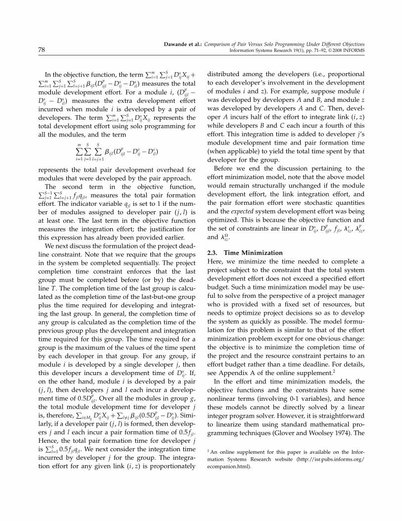
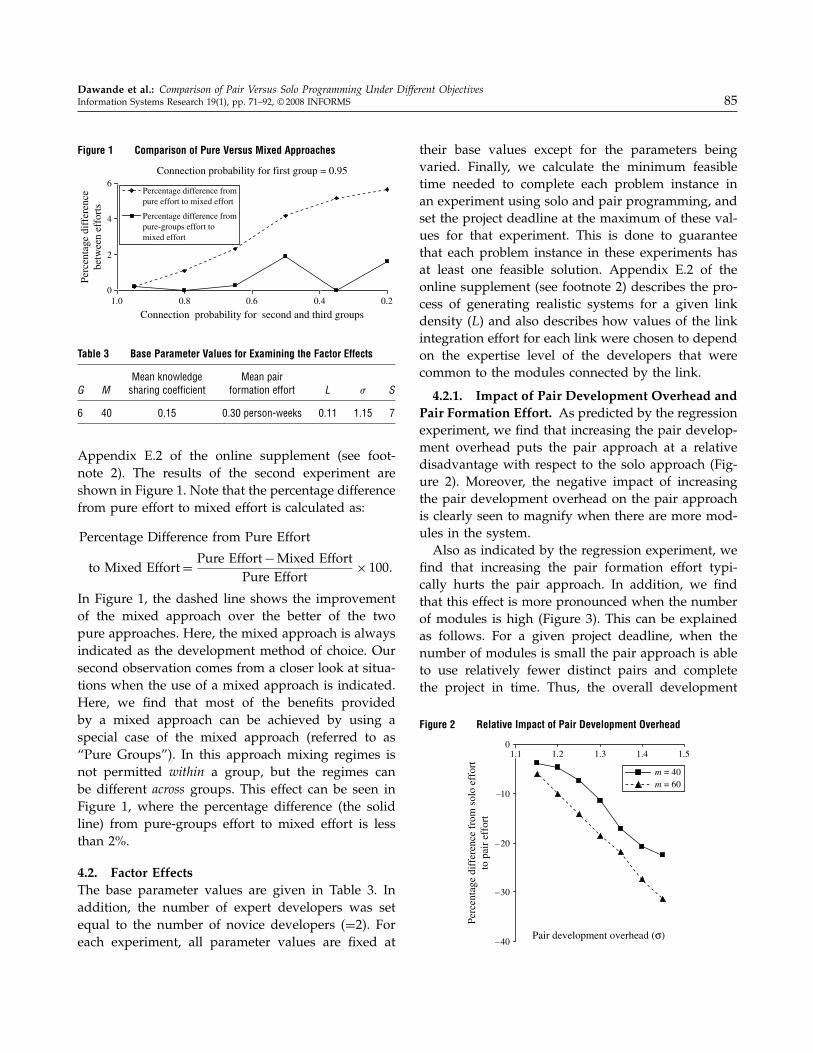
4.2.1. Impact of Pair Development Overhead andPair Formation Effort. As predicted by the regressionexperiment, we find that increasing the pair develop-ment overhead puts the pair approach at a relativedisadvantage with respect to the solo approach (Fig-ure 2). Moreover, the negative impact of increasingthe pair development overhead on the pair approachis clearly seen to magnify when there are more mod-ules in the system.Also as indicated by the regression experiment, we
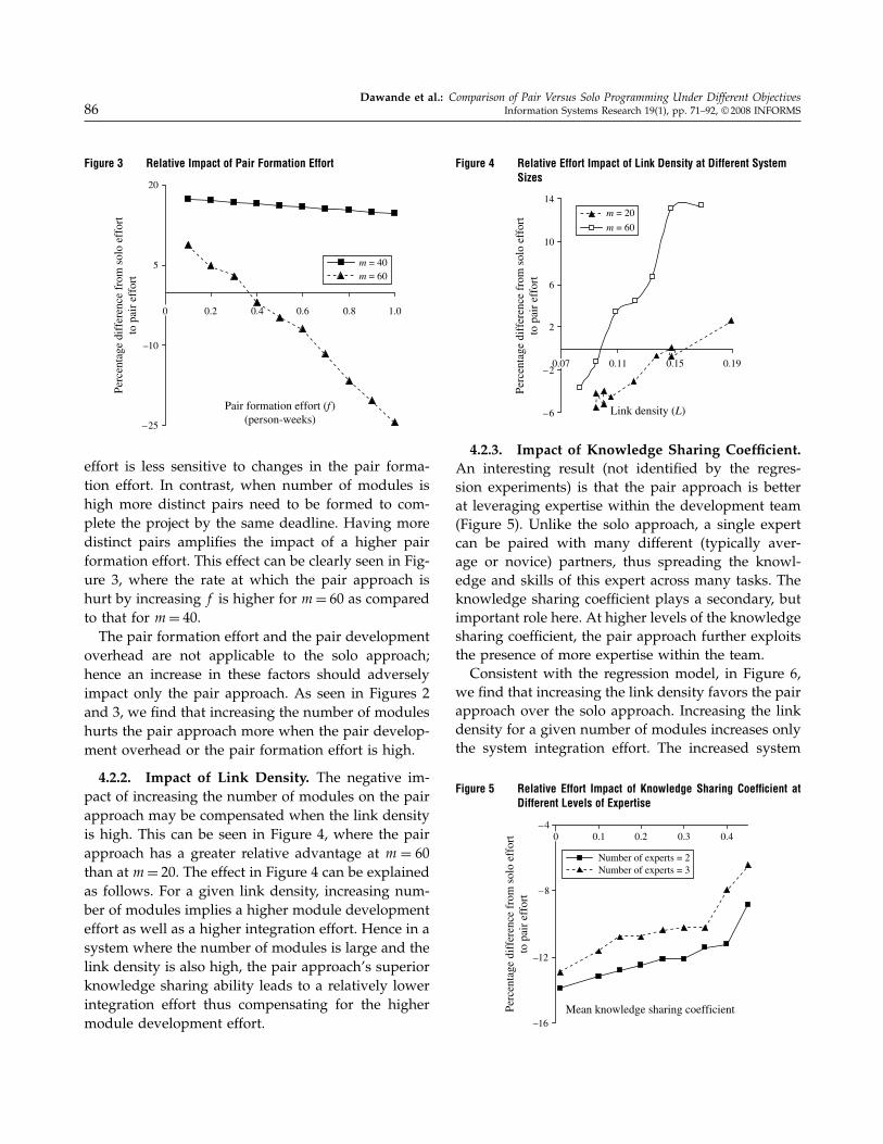
find that increasing the pair formation effort typi-cally hurts the pair approach. In addition, we findthat this effect is more pronounced when the numberof modules is high (Figure 3). This can be explainedas follows. For a given project deadline, when thenumber of modules is small the pair approach is ableto use relatively fewer distinct pairs and completethe project in time. Thus, the overall development
Figure 2 Relative Impact of Pair Development Overhead
–10
–20
–30
–40
01.2 1.3 1.4 1.5
Pair development overhead (σ)
Perc
enta
ge d
iffe
renc
e fr
om s
olo
effo
rtto
pai
r ef
fort
1.1
m = 40m = 60
Dawande et al.: Comparison of Pair Versus Solo Programming Under Different Objectives86 Information Systems Research 19(1), pp. 71–92, © 2008 INFORMS
Figure 3 Relative Impact of Pair Formation Effort
–25
–10
5
20
0.2 0.4 0.6 0.8 1.0
Pair formation effort (f )(person-weeks)
Perc
enta
ge d
iffe
renc
e fr
om s
olo
effo
rtto
pai
r ef
fort
m = 40m = 60
0
effort is less sensitive to changes in the pair forma-tion effort. In contrast, when number of modules ishigh more distinct pairs need to be formed to com-plete the project by the same deadline. Having moredistinct pairs amplifies the impact of a higher pairformation effort. This effect can be clearly seen in Fig-ure 3, where the rate at which the pair approach ishurt by increasing f is higher for m= 60 as comparedto that for m= 40.The pair formation effort and the pair development
overhead are not applicable to the solo approach;hence an increase in these factors should adverselyimpact only the pair approach. As seen in Figures 2and 3, we find that increasing the number of moduleshurts the pair approach more when the pair develop-ment overhead or the pair formation effort is high.
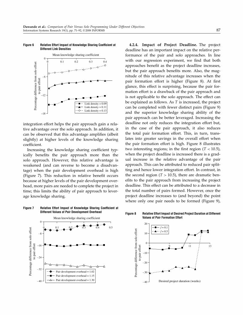
4.2.2. Impact of Link Density. The negative im-pact of increasing the number of modules on the pairapproach may be compensated when the link densityis high. This can be seen in Figure 4, where the pairapproach has a greater relative advantage at m = 60than at m= 20. The effect in Figure 4 can be explainedas follows. For a given link density, increasing num-ber of modules implies a higher module developmenteffort as well as a higher integration effort. Hence in asystem where the number of modules is large and thelink density is also high, the pair approach’s superiorknowledge sharing ability leads to a relatively lowerintegration effort thus compensating for the highermodule development effort.
Figure 4 Relative Effort Impact of Link Density at Different SystemSizes
–6
–2
2
6
10
14
0.11 0.15 0.19
Link density (L)
Perc
enta
ge d
iffe
renc
e fr
om s
olo
effo
rtto
pai
r ef
fort
m = 20
m = 60
0.07
4.2.3. Impact of Knowledge Sharing Coefficient.An interesting result (not identified by the regres-sion experiments) is that the pair approach is betterat leveraging expertise within the development team(Figure 5). Unlike the solo approach, a single expertcan be paired with many different (typically aver-age or novice) partners, thus spreading the knowl-edge and skills of this expert across many tasks. Theknowledge sharing coefficient plays a secondary, butimportant role here. At higher levels of the knowledgesharing coefficient, the pair approach further exploitsthe presence of more expertise within the team.Consistent with the regression model, in Figure 6,
we find that increasing the link density favors the pairapproach over the solo approach. Increasing the linkdensity for a given number of modules increases onlythe system integration effort. The increased system
Figure 5 Relative Effort Impact of Knowledge Sharing Coefficient atDifferent Levels of Expertise
–16
–12
–8
–40.1 0.2 0.3 0.4
Mean knowledge sharing coefficientPerc
enta
ge d
iffe
renc
e fr
om s
olo
effo
rtto
pai
r ef
fort
Number of experts = 2Number of experts = 3
0
Dawande et al.: Comparison of Pair Versus Solo Programming Under Different ObjectivesInformation Systems Research 19(1), pp. 71–92, © 2008 INFORMS 87
Figure 6 Relative Effort Impact of Knowledge Sharing Coefficient atDifferent Link Densities
0.1 0.2 0.3 0.4
Mean knowledge sharing coefficient
Link density = 0.09Link density = 0.11Link density = 0.13
–18
–12
–6
0
Perc
enta
ge d
iffe
renc
e fr
om s
olo
effo
rtto
pai
r ef
fort
0
integration effort helps the pair approach gain a rela-tive advantage over the solo approach. In addition, itcan be observed that this advantage amplifies (albeitslightly) at higher levels of the knowledge sharingcoefficient.Increasing the knowledge sharing coefficient typ-
ically benefits the pair approach more than thesolo approach. However, this relative advantage isweakened (and can reverse to become a disadvan-tage) when the pair development overhead is high(Figure 7). This reduction in relative benefit occursbecause at higher levels of the pair development over-head, more pairs are needed to complete the project intime; this limits the ability of pair approach to lever-age knowledge sharing.
Figure 7 Relative Effort Impact of Knowledge Sharing Coefficient atDifferent Values of Pair Development Overhead
–40
–32
–24
–16
–8
0
0.1 0.2 0.3 0.4 0.5
Mean knowledge sharing coefficient
Perc
enta
ge d
iffe
renc
e fr
om s
olo
effo
rtto
pai
r ef
fort
Pair development overhead = 1.02
Pair development overhead = 1.15
Pair development overhead = 1.30
0
4.2.4. Impact of Project Deadline. The projectdeadline has an important impact on the relative per-formance of the pair and solo approaches. In linewith our regression experiment, we find that bothapproaches benefit as the project deadline increases,but the pair approach benefits more. Also, the mag-nitude of this relative advantage increases when thepair formation effort is higher (Figure 8). At firstglance, this effect is surprising, because the pair for-mation effort is a drawback of the pair approach andis not applicable to the solo approach. The effect canbe explained as follows. As T is increased, the projectcan be completed with fewer distinct pairs (Figure 9)and the superior knowledge sharing ability of thepair approach can be better leveraged. Increasing thedeadline not only reduces the integration effort but,in the case of the pair approach, it also reducesthe total pair formation effort. This, in turn, trans-lates into greater savings in the overall effort whenthe pair formation effort is high. Figure 8 illustratestwo interesting regions; in the first region (T < 10�5),when the project deadline is increased there is a grad-ual increase in the relative advantage of the pairapproach. This can be attributed to reduced pair split-ting and hence lower integration effort. In contrast, inthe second region (T > 10�5), there are dramatic ben-efits to the pair approach from increasing the projectdeadline. This effect can be attributed to a decrease inthe total number of pairs formed. However, once theproject deadline increases to (and beyond) the pointwhere only one pair needs to be formed (Figure 9),
Figure 8 Relative Effort Impact of Desired Project Duration at DifferentValues of Pair Formation Effort
–40
–30
–20
–10
0
10
20
9 11 13
Desired project duration (weeks)
Perc
enta
ge d
iffe
renc
e fr
om s
olo
effo
rtto
pai
r ef
fort
f = 0.1
f = 0.5
7
Dawande et al.: Comparison of Pair Versus Solo Programming Under Different Objectives88 Information Systems Research 19(1), pp. 71–92, © 2008 INFORMS
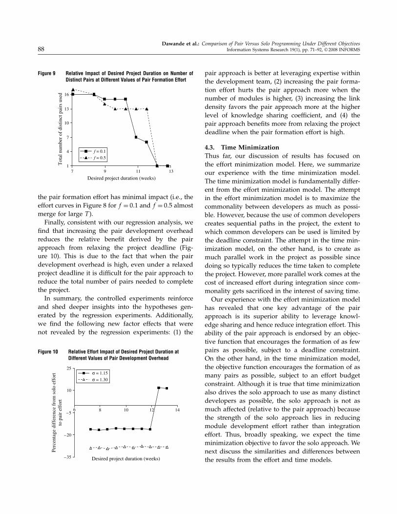
Figure 9 Relative Impact of Desired Project Duration on Number ofDistinct Pairs at Different Values of Pair Formation Effort
1
4
7
10
13
16
7 11 13
Desired project duration (weeks)
Tot
al n
umbe
r of
dis
tinct
pai
rs u
sed
f = 0.1
f = 0.5
9
the pair formation effort has minimal impact (i.e., theeffort curves in Figure 8 for f = 0�1 and f = 0�5 almostmerge for large T ).Finally, consistent with our regression analysis, we
find that increasing the pair development overheadreduces the relative benefit derived by the pairapproach from relaxing the project deadline (Fig-ure 10). This is due to the fact that when the pairdevelopment overhead is high, even under a relaxedproject deadline it is difficult for the pair approach toreduce the total number of pairs needed to completethe project.In summary, the controlled experiments reinforce
and shed deeper insights into the hypotheses gen-erated by the regression experiments. Additionally,we find the following new factor effects that werenot revealed by the regression experiments: (1) the
Figure 10 Relative Effort Impact of Desired Project Duration atDifferent Values of Pair Development Overhead
–35
–20
–5
10
25
8 10 12 14
Desired project duration (weeks)
Perc
enta
ge d
iffe
renc
e fr
om s
olo
effo
rtto
pai
r ef
fort
6
σ = 1.15
σ = 1.30
pair approach is better at leveraging expertise withinthe development team, (2) increasing the pair forma-tion effort hurts the pair approach more when thenumber of modules is higher, (3) increasing the linkdensity favors the pair approach more at the higherlevel of knowledge sharing coefficient, and (4) thepair approach benefits more from relaxing the projectdeadline when the pair formation effort is high.
4.3. Time MinimizationThus far, our discussion of results has focused onthe effort minimization model. Here, we summarizeour experience with the time minimization model.The time minimization model is fundamentally differ-ent from the effort minimization model. The attemptin the effort minimization model is to maximize thecommonality between developers as much as possi-ble. However, because the use of common developerscreates sequential paths in the project, the extent towhich common developers can be used is limited bythe deadline constraint. The attempt in the time min-imization model, on the other hand, is to create asmuch parallel work in the project as possible sincedoing so typically reduces the time taken to completethe project. However, more parallel work comes at thecost of increased effort during integration since com-monality gets sacrificed in the interest of saving time.Our experience with the effort minimization model
has revealed that one key advantage of the pairapproach is its superior ability to leverage knowl-edge sharing and hence reduce integration effort. Thisability of the pair approach is endorsed by an objec-tive function that encourages the formation of as fewpairs as possible, subject to a deadline constraint.On the other hand, in the time minimization model,the objective function encourages the formation of asmany pairs as possible, subject to an effort budgetconstraint. Although it is true that time minimizationalso drives the solo approach to use as many distinctdevelopers as possible, the solo approach is not asmuch affected (relative to the pair approach) becausethe strength of the solo approach lies in reducingmodule development effort rather than integrationeffort. Thus, broadly speaking, we expect the timeminimization objective to favor the solo approach. Wenext discuss the similarities and differences betweenthe results from the effort and time models.
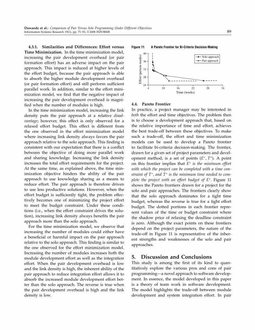
Dawande et al.: Comparison of Pair Versus Solo Programming Under Different ObjectivesInformation Systems Research 19(1), pp. 71–92, © 2008 INFORMS 89
4.3.1. Similarities and Differences: Effort versusTime Minimization. In the time minimization model,increasing the pair development overhead (or pairformation effort) has an adverse impact on the pairapproach. This impact is reduced at higher levels ofthe effort budget, because the pair approach is ableto absorb the higher module development overhead(or pair formation effort) and still perform sufficientparallel work. In addition, similar to the effort mini-mization model, we find that the negative impact ofincreasing the pair development overhead is magni-fied when the number of modules is high.In the time minimization model, increasing the link
density puts the pair approach at a relative disad-vantage; however, this effect is only observed for arelaxed effort budget. This effect is different fromthe one observed in the effort minimization modelwhere increasing link density always favors the pairapproach relative to the solo approach. This finding isconsistent with our expectation that there is a conflictbetween the objective of doing more parallel workand sharing knowledge. Increasing the link densityincreases the total effort requirements for the project.At the same time, as explained above, the time min-imization objective hinders the ability of the pairapproach to use knowledge sharing as a means toreduce effort. The pair approach is therefore drivento use less productive solutions. However, when theeffort budget is sufficiently tight, the problem effec-tively becomes one of minimizing the project effortto meet the budget constraint. Under these condi-tions (i.e., when the effort constraint drives the solu-tion), increasing link density always benefits the pairapproach more than the solo approach.For the time minimization model, we observe that
increasing the number of modules could either havea beneficial or harmful impact on the pair approachrelative to the solo approach. This finding is similar tothe one observed for the effort minimization model.Increasing the number of modules increases both themodule development effort as well as the integrationeffort. When the pair development overhead is lowand the link density is high, the inherent ability of thepair approach to reduce integration effort allows it toabsorb the increased module development effort bet-ter than the solo approach. The reverse is true whenthe pair development overhead is high and the linkdensity is low.
Figure 11 A Pareto Frontier for Bi-Criteria Decision-Making
24
28
32
36
40
4 10 16 22 28 34
Time (weeks)
Eff
ort (
pers
on-w
eeks
)
Solo approachPair approach
4.4. Pareto FrontierIn practice, a project manager may be interested inboth the effort and time objectives. The problem thenis to choose a development approach that, based onthe relative importance of time and effort, achievesthe best trade-off between these objectives. To makesuch a trade-off, the effort and time minimizationmodels can be used to develop a Pareto frontierto facilitate bi-criteria decision-making. The frontier,drawn for a given set of project parameters and devel-opment method, is a set of points (E∗�T ∗). A pointon this frontier implies that E∗ is the minimum effortwith which the project can be completed with a time con-straint of T ∗, and T ∗ is the minimum time needed to com-plete the project with an effort budget of E∗. Figure 11shows the Pareto frontiers drawn for a project for thesolo and pair approaches. The frontiers clearly showthat the solo approach dominates for a tight timebudget, whereas the reverse is true for a tight effortbudget. The dotted portions in each frontier repre-sent values of the time or budget constraint wherethe shadow price of relaxing the deadline constraintis zero. Although the exact points on these frontiersdepend on the project parameters, the nature of thetrade-off in Figure 11 is representative of the inher-ent strengths and weaknesses of the solo and pairapproaches.
5. Discussion and ConclusionsThis study is among the first of its kind to quan-titatively explore the various pros and cons of pairprogramming—a novel approach to software develop-ment. In essence, the model developed in this paperis a theory of team work in software development.The model highlights the trade-off between moduledevelopment and system integration effort. In pair
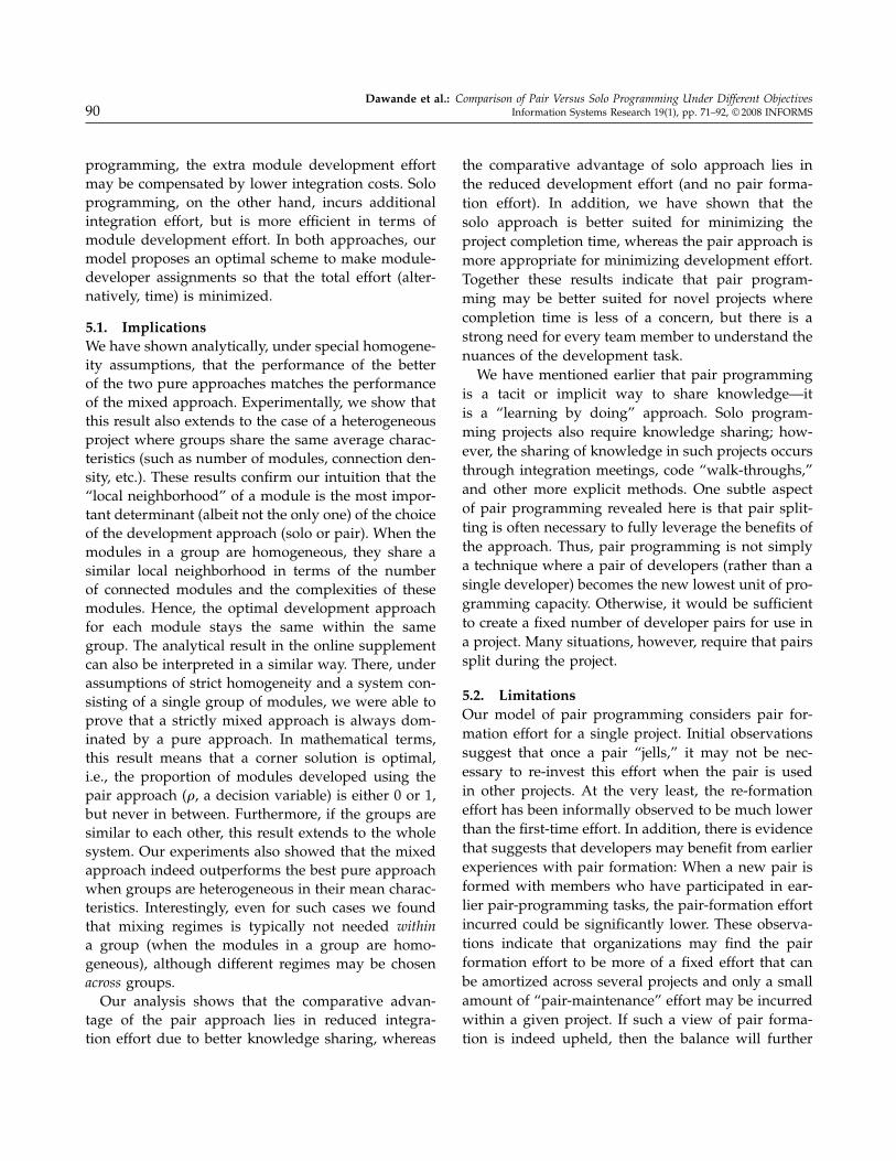
Dawande et al.: Comparison of Pair Versus Solo Programming Under Different Objectives90 Information Systems Research 19(1), pp. 71–92, © 2008 INFORMS
programming, the extra module development effortmay be compensated by lower integration costs. Soloprogramming, on the other hand, incurs additionalintegration effort, but is more efficient in terms ofmodule development effort. In both approaches, ourmodel proposes an optimal scheme to make module-developer assignments so that the total effort (alter-natively, time) is minimized.
5.1. ImplicationsWe have shown analytically, under special homogene-ity assumptions, that the performance of the betterof the two pure approaches matches the performanceof the mixed approach. Experimentally, we show thatthis result also extends to the case of a heterogeneousproject where groups share the same average charac-teristics (such as number of modules, connection den-sity, etc.). These results confirm our intuition that the“local neighborhood” of a module is the most impor-tant determinant (albeit not the only one) of the choiceof the development approach (solo or pair). When themodules in a group are homogeneous, they share asimilar local neighborhood in terms of the numberof connected modules and the complexities of thesemodules. Hence, the optimal development approachfor each module stays the same within the samegroup. The analytical result in the online supplementcan also be interpreted in a similar way. There, underassumptions of strict homogeneity and a system con-sisting of a single group of modules, we were able toprove that a strictly mixed approach is always dom-inated by a pure approach. In mathematical terms,this result means that a corner solution is optimal,i.e., the proportion of modules developed using thepair approach (2, a decision variable) is either 0 or 1,but never in between. Furthermore, if the groups aresimilar to each other, this result extends to the wholesystem. Our experiments also showed that the mixedapproach indeed outperforms the best pure approachwhen groups are heterogeneous in their mean charac-teristics. Interestingly, even for such cases we foundthat mixing regimes is typically not needed withina group (when the modules in a group are homo-geneous), although different regimes may be chosenacross groups.Our analysis shows that the comparative advan-
tage of the pair approach lies in reduced integra-tion effort due to better knowledge sharing, whereas
the comparative advantage of solo approach lies inthe reduced development effort (and no pair forma-tion effort). In addition, we have shown that thesolo approach is better suited for minimizing theproject completion time, whereas the pair approach ismore appropriate for minimizing development effort.Together these results indicate that pair program-ming may be better suited for novel projects wherecompletion time is less of a concern, but there is astrong need for every team member to understand thenuances of the development task.We have mentioned earlier that pair programming
is a tacit or implicit way to share knowledge—itis a “learning by doing” approach. Solo program-ming projects also require knowledge sharing; how-ever, the sharing of knowledge in such projects occursthrough integration meetings, code “walk-throughs,”and other more explicit methods. One subtle aspectof pair programming revealed here is that pair split-ting is often necessary to fully leverage the benefits ofthe approach. Thus, pair programming is not simplya technique where a pair of developers (rather than asingle developer) becomes the new lowest unit of pro-gramming capacity. Otherwise, it would be sufficientto create a fixed number of developer pairs for use ina project. Many situations, however, require that pairssplit during the project.
5.2. LimitationsOur model of pair programming considers pair for-mation effort for a single project. Initial observationssuggest that once a pair “jells,” it may not be nec-essary to re-invest this effort when the pair is usedin other projects. At the very least, the re-formationeffort has been informally observed to be much lowerthan the first-time effort. In addition, there is evidencethat suggests that developers may benefit from earlierexperiences with pair formation: When a new pair isformed with members who have participated in ear-lier pair-programming tasks, the pair-formation effortincurred could be significantly lower. These observa-tions indicate that organizations may find the pairformation effort to be more of a fixed effort that canbe amortized across several projects and only a smallamount of “pair-maintenance” effort may be incurredwithin a given project. If such a view of pair forma-tion is indeed upheld, then the balance will further
Dawande et al.: Comparison of Pair Versus Solo Programming Under Different ObjectivesInformation Systems Research 19(1), pp. 71–92, © 2008 INFORMS 91
tilt toward the use of pair programming for softwaredevelopment—implying that the results in this paperat low values of the pair formation effort may be morerepresentative.A limitation of the model presented here is that it
emphasizes total system development effort (and sys-tem development time) as the only criteria to comparethe solo and pair programming approaches. How-ever, there are other aspects of pair programming thatcould be beneficial. For example, pair programming,through pair formation and pair splitting, may havesocial and psychological benefits. If applied effec-tively, it could reduce the tedium of software devel-opment and improve developer morale.On the other hand, there are potential “incentive”
problems in implementing pair programming thatthis study did not consider; specifically, what effectsdoes joint code ownership have on the quality of theoutput? Unless incentive mechanisms are correctlyin place, it is possible that there is some extent of“free-riding” when a developer pair jointly developscode. This may be one of the reasons why pairs withnonsymmetric experience and abilities are formed,e.g., partnering a junior programmer with a seniorarchitect. In such partnerships, the two individualscontribute in different ways, e.g., the senior architectprovides high-level architectural expertise and eval-uates the code for quality and functionality, whereasthe junior programmer contributes by working outdetails and actually writing the code. If two devel-opers of equal skill and experience are paired, it ispossible that incentive issues become perverse andfree-riding becomes a problem.
5.3. ConclusionsIn this paper, we developed an analytical model tooptimize module-developer assignments in softwaredevelopment with the objective of minimizing thetotal system development effort (or total develop-ment time). The main purpose of the study was tocompare the optimal assignments under two regimes:solo programming and pair programming. Using acombination of experimental and analytical resultswe were able to provide several recommendationsfor software development practice. A useful resultof our analysis was that there is not much supportfor simultaneously operating in both the regimes,
solo as well as pair, within a group. However, whenthe groups are sufficiently heterogeneous in theiraverage characteristics, it may sometimes be opti-mal to choose different regimes across groups forthe same software project. We proposed an accuratemeans of predicting the superior approach for a givenproject based upon average project parameters val-ues (module complexity, connectivity, and pair forma-tion effort) that should be relatively easy to estimatefor a given project. Because the prediction techniquewas based on strict homogeneity assumptions, weran extensive numerical experiments (in which theseassumptions were relaxed) to gain insights into con-ditions in which the solo or the pair approach wouldbe preferred. When the knowledge sharing betweenthe developers is efficient or when the functionaldependence between the system modules is high, thepair approach is preferable over the solo approach.The pair approach also appears to be better than thesolo approach at distributing scarce expertise acrossmore development tasks (by forming more pairs withexpert developers). If the pair development overheador the pair formation effort is high, the solo approachis more suitable. Projects with a tight deadline are lesssuited for pair programming.
ReferencesAhuja, R. K., J. B. Orlin, A. Tiwari. 2000. A descent genetic algo-
rithm for the quadratic assignment problem. Comput. Oper. Res.27 917–934.
Ambler, S. W. 2002. Agile Modeling� Effective Practices for eXtremeProgramming and the Unified Process. John Wiley & Sons, Inc.,New York.
Astels, D., G. Miller, M. Novak. 2002. A Practical Guide to ExtremeProgramming. Prentice Hall, Upper Saddle River, NJ.
Baecker, R., J. Grudin, W. Buxton, S. Greenberg. 1995. Readingsin Human-Computer Interaction� Toward the Year 2000. MorganKaufmann Publishers, Inc., San Francisco.
Beck, K. 2000. Extreme Programming Explained� Embrace Change.Addison-Wesley, Boston.
Beck, K., M. Fowler. 2001. Planning Extreme Programming. Addison-Wesley, Boston.
Benedicenti, L., R. Paranjape. 2001. Using extreme programming forknowledge transfer. Proc. 2nd Internat. Conf. eXtreme Program-ming and Agile Processes in Software Engrg. �XP2001�, Villasim-ius, Sardinia, Italy.
Brown, J. S., P. Duguid. 1991. Organizational learning and commu-nities of practice: Toward a unified view of working, learningand innovation. Organ. Sci. 2(1) 40–57.
Burrill, D. 1997. Modeling and interpreting interactions in multipleregression. Available at http://www.minitab.com/.
Dawande et al.: Comparison of Pair Versus Solo Programming Under Different Objectives92 Information Systems Research 19(1), pp. 71–92, © 2008 INFORMS
Cockburn, A., J. Highsmith. 2001. Agile software development: Thepeople factor. Computer (November) 131–133.
Cockburn, A., L. Williams. 2000. The costs and benefits of pair pro-gramming. Proc. 1st Internat. Conf. eXtreme Programming andFlexible Processes in Software Engrg. (XP2000). Cagliari, Sardinia,Italy.
Curtis, B., H. Krasner, N. Iscoe. 1988. A field study of the soft-ware design process for large systems. Comm. ACM 31(11)1268–1287.
Dingsoyr, T. 2002. Knowledge management in medium-sizedsoftware consulting companies. Ph.D. thesis, Department ofComputer and Information Science, Norwegian University ofScience and Technology, Trondheim, Norway.
Drezner, Z. 2003. A new genetic algorithm for the quadratic assign-ment problem. Informs J. Comput. 15(3) 320–330.
Erdogmus, H., L. Williams. 2003. The economics of software devel-opment by pair programmers. Engrg. Economist 48(4) 283–319.
Fleurent, C., J. A. Ferland. 1994. Genetic hybrids for the quadraticassignment problem. P. Pardalos, H. Wolkowicz, eds. QuadraticAssignment and Related Problems, DIMACS Series in DiscreteMathematics and Theoretical Computer Science, 16 173–187.
Garey, M. R., D. S. Johnson. 1979. Computers and Intractability�A Guide to the Theory of NP-Completeness. W. H. Freeman & Co.,New York.
Glover, F., E. Woolsey. 1974. Converting the 0-1 polynomial pro-gramming problem to a 0-1 linear program. Oper. Res. 22(1)180–182.
Goldberg, D. E. 1989. Genetic Algorithms in Search, Optimization andMachine Learning. Addison-Wesley, Wokingham, UK.
Grunbacher, P., C. Hofer. 2003. Complementing XP with require-ments negotiation. Proc. 4th Internat. Conf. eXtreme Programmingand Agile Processes in Software Engrg. (XP2003). Genova, Italy.
Hailpern, B., P. Santhanam. 2002. Software debugging, testing andverification. IBM Systems J.� Software Testing and Verification41(1).
Highsmith, J., A. Cockburn. 2001. Agile software development: Thebusiness of innovation. IEEE Comput. (September) 120–122.
Ippolito, B., E. Murman. 2001. Improving the software upgradevalue stream. Lean Aerospace Initiative (LAI) Monograph,Working Paper ESD-WP-2002-02, Engineering Systems Divi-sion, Massachusetts Institute of Technology.
Kleinbaum, D. G., L. L. Kupper, K. E. Muller. 1998. Appliedregression analysis and other multivariate methods. PWS-Kent,Boston.
Kuppuswami, S., K. Vivekandanam, P. Ramaswamy, P. Rodrigues.2003. The effects of individual XP practices on softwaredevelopment effort. ACM SIGSOFT Software Engrg. Notes28(6, November) 6–13.
Lui, K. M., K. C. C. Chan. 2004. A cognitive model for solo pro-gramming and pair programming. Proc. 3rd IEEE Internat. Conf.Cognitive Informatics �ICCI’04�, Victoria, Canada. IEEE ComputerSociety, Washington D.C. 94–102.
Meixell, M. J., M. Nunez, A. Talalayevsky. 2006. Activity structuresin a project-based environment: A coordination theory perspec-tive. IEEE Trans. Engrg. Management 53(2, May) 285–296.
Nawrocki, J., A. Wojciechowski. 2001. Experimental evaluation ofpair programming. Proc. 12th Eur. Software Control and Met-rics Conf., London, UK, Shaker Publishing BV, Maastricht, TheNetherlands. 269–276.
Nielsen, J. 1993. Usability Engineering. Academic Press, Boston.Nosek, J. T. 1998. The cast for collaborative programming. Comm.
ACM 41(3) 105–108.Pressman, R. 1992. Software Engineering� A Practitioner’s Approach.
McGraw-Hill, New York.Shukla, A. 2002. Pair programming and the factors affecting Brook’s
law. Master’s thesis, North Carolina State University, Raleigh,NC.
Succi, G., M. Stefanovic, W. Pedrycz. 2001. Quantitative assessmentof extreme programming practices. Proc. 2001 Canadian Conf.Electrical and Comput. Engrg. Toronto. IEEE, Washington, D.C.81–86.
Tate, D. M., A. E. Smith. 1995. A genetic approach to the quadraticassignment problem. Comput. Oper. Res. 22 73–83.
Waltz, D., B. Curtis, J. Elam. 1993. Inside a software design team:Knowledge acquisition, sharing and integration. Comm. ACM36(10) 62–77.
Wells, D. 2003. Extreme programming: A gentle introduction. Avail-able at http://extremeprogramming.org., January 26.
Williams, L., R. Kessler. 2003. Pair Programming Illuminated.Addison-Wesley.
Williams, L., R. Kessler, W. Cunningham, R. Jeffries. 2000.Strengthening the case for pair-programming. IEEE Software17(4, July/August) 19–25.
Wood, A., W. Kleb. 2002. Extreme programming in a research envi-ronment. Technical report, NASA Langley Research Center,Hampton, VA.
Yu, C. H. 2000. An overview of remedial tools for collinearity inSAS. Proc. 2000 Western Users of SAS Software Conf., Scottsdale,AZ, SAS Software, Cary, NC, 196–201.