A COMPARISON OF NUMERICAL IMPLEMENTATIONS OF THEEIGENSTATE EXPANSION METHOD FOR QUANTUM MOLECULAR

DYNAMICS SIMULATIONS

PETER ARBENZ† , OLIVER BROKER† , OSCAR CHINELLATO† , WALTER GANDER† , ROMAN

GEUS† , AND ROLF STREBEL†

Abstract. We investigate the efficient computation of a few of the lowest eigenvalues of a symmetriceigenvalue problem occurring in quantum dynamical molecular simulations. The large sparse system oforder n3 is highly structured such that its multiplication with a vector costs O(n3 logn) floating pointoperations only.

We compare a number of eigensolvers: subspace iteration, two variants of the restarted Lanczos algo-rithm, among them ARPACK, the Jacobi-Davidson algorithm and the classical algorithms from LAPACKfor full matrices. Some of them are applied with a shift-and-invert spectral transformation. The arisingsystems of equations are solved by the preconditioned conjugate gradient method for which new efficientADI-type preconditioners are proposed and analyzed.

Key words. quantum molecular dynamics, eigenfunction expansion method, sparse eigenvalue prob-lem, preconditioned conjugate gradient method.

AMS subject classifications. 65F10, 65F15

1. Introduction. Numerical methods derived from classical molecular (CM) dynam-ics allow one to perform dynamics on a nanosecond time scale for systems involving tensof thousands of atoms. However, classical (as opposed to quantum) molecular dynam-ics prevents the study of processes like proton transfers and the making and breaking ofchemical bonds that are of much interest in enzyme reactions or other biochemical pro-cesses. Unfortunately, the complexity of a fully quantum mechanical (QM) treatment ofchemical systems with more than a very small number of degrees of freedom is far be-yond the capacity of nowadays computers. Therefore, in molecular dynamics computersimulation packages like GROMOS [6, 13], mixed QM/CM simulation schemes are imple-mented in which a small part of the degrees of freedom are treated quantum mechanically,generally regarding light particles such as electrons and protons that are directly involvedin the reactive molecular rearrangement, while the many more degrees of freedom of theenvironment of the reactive site are treated classically.

The QMD method is based on so-called real-time-path-integral techniques [16], whichare aimed at obtaining the time evolution of a state function ψ under the influence of theHamilton operator H. If the Hamilton operator

Hψ = (K + V)ψ = − ~2

2m∆ψ + V (ψ,x).

in the time-dependent Schrodinger equation

i~∂ψ

∂t= Hψ(t)(1.1)

does not change with time, the state ψ at time t is given formally by

ψ(t) = exp(− ihHt)ψ(0) = exp(− i

h(K + V)t)ψ(0).(1.2)

†Swiss Federal Institute of Technology (ETH), Institute of Scientific Computing, 8092 Zurich, Switzer-land ([arbenz,broeker,chinellato,gander,geus,strebel]@inf.ethz.ch)

ETH Zurich, CS Technical Report #333, Institute of Scientific Computing, January 13, 2000

2 ARBENZ, BROKER, CHINELLATO, GANDER, GEUS, AND STREBEL

There are two problematic aspects regarding the Hamilton operator: the kinetic energyoperatorK is non-local in the coordinate representation, and the kinematic energy operatorK and the potential energy operator V do not commute. In the literature a number ofschemes have been proposed and tested to integrate (1.2). These are based on so-calledsplit operator formulae and the use of the fast Fourier transforms (FFT) to obtain a localkinetic energy operator in momentum space. In [5], Billeter and van Gunsteren found thatan integration technique involving an eigenfunction expansion of ψ(t) is suited for mixedQD/MD simulations. If {φk}∞k=1 is the complete set of eigenfunctions of H,

Hφk = λkφk,

we can expand the state ψ as

ψ =∞Xk=1

αkφk, αk = 〈φk, ψ〉.(1.3)

As the Schrodinger equation (1.1) can be solved if the initial state equals an eigenfunctionof H, φk(t) = φk(0)e−(i/~)λit, we get for an initial state of the form (1.3)

ψ(t) =Xk

〈φk, ψ(t)〉φk =Xk

〈φk, exp(− ithH)ψ(0)〉φk =

Xk

e−iλkt/h〈φk, ψ(0)〉φk

Since the state ψ takes on only low energy levels with non-negligible probability, just afew of the lowest eigenvalues λk of H(t) are needed to get accurate approximations. If theHamilton operator is time-dependent, an approximate solution is obtained by linearization.

We investigate three dimensional as well as simplified one-dimensional model problems.In the one-dimensional case ψ in (1.1) is represented as a Fourier polynomial of order n.In three dimensions ψ is represented as the tensor product of Fourier polynomial of ordern. The resulting symmetric large sparse matrix eigenvalue problems thus have orders nd

where d is the number of dimensions.Solving the large eigenvalue problem with the QR algorithm as available in LA-

PACK [1] requires O(n3d) floating point operations and O(n2d) memory locations whichmakes this approach infeasible for approximations in 3D of even moderate orders n. Wetherefore investigate algorithms that are adapted to sparse large scale eigenvalue prob-lems in that they access the system matrix only by means of matrix-vector products. Thespecial matrix structure admits using FFT techniques such that a matrix-vector productcosts only O(n log(n)) floating point operations.

We solve the resulting symmetric large sparse matrix eigenvalue problems by twovariants of the restarted Lanczos algorithm [17], by subspace iteration [20] and by theJacobi-Davidson algorithm [24, 9]. The latter two algorithms have been chosen as theycan naturally exploit good initial guesses for the eigenvectors. This is important in QDsimulations where in each of thousands of time steps an eigenvalue problem has to besolved that differs only little from the one of the previous point in time. The system ofequations that arise with the shift-and-invert spectral transformation (subspace iterationand Jacobi-Davidson algorithm) are solved with the preconditioned conjugate gradientmethod. We propose a new preconditioner to enhance convergence.

The outline of the paper is as follows. In section 2 we investigate the simplified 1Dproblem followed by numerical experiments in section 3. In section 4 we turn to the theoryfor the 3D eigenvalue problem. Numerical experiments are presented in 5. We close withsome remarks in section 6.ETH Zurich, CS Technical Report #333, Institute of Scientific Computing, January 13, 2000

IMPLEMENTATIONS OF THE EIGENSTATE EXPANSION METHOD 3

2. The 1D problem. The Schrodinger equation (1.1) for a one-dimensional particleof mass m is given by

− ~2

2mu′′(x) + V (x)u(x) = λu(x), 0 < x < 2π,(2.1)

with periodic boundary conditions. We approximate u(x) as a Fourier polynomial of ordern, n even (mostly n = 2q for some q ∈ N),

u(x) =

n2X

k=−n2

+1

ckeikx,(2.2)

whence

u′′(x) =

n2X

k=−n2

+1

−k2ckeikx.

Solving (2.1) by collocation at the points xj = 2πj/n, j = 0, . . . , n − 1 yields the nequations

n2X

k=−n2

+1

~

2

2mk2 + V (xj)− λ

!cke

ikxj = 0, j = 0, . . . , n− 1.(2.3)

Noting that e−ikxj = ei(n−k)xj and identifying c−k with cn−k eq. (2.3) becomes

n−1Xk=0

~

2

2mmin(k, n−k)2 + V (xj)− λ

!cke

ikxj = 0, j = 0, . . . , n− 1.(2.4)

The matrix form of these equations is

(FnKn + VnFn − λFn)c = 0,(2.5)

where,

Kn :=~

2

2mdiag

�0, 1, . . . , (

n

2)2, (

n

2− 1)2, . . . , 1

�∈ Rn×n,

Vn = diag (V (x0), . . . , V (xn−1)) ∈ Rn×n,Fn = ((ωjkn ))nj,k=0 ∈ Cn×n, ωn = e2πi/n.

Fn is the n-by-n Fourier matrix [18]. Notice, that FnF ∗n = nIn, In the n-by-n identitymatrix, such that F−1

n = 1nF∗n . Here, F ∗n denotes the conjugate transpose of Fn. Set

x := Fnc to get the eigenvalue problem

(Hn + Vn)x := (FnKnF−1n + Vn)x = λx.(2.6)

We haveLemma 2.1. The matrix Hn := FnKnF

−1n is real symmetric and circulant.

Thus, the matrix An := FnKnF−1n + Vn is real symmetric und up to the diagonal

circulant as well. This implies that its eigenvalues are real and the eigenvectors forman orthonormal basis of Rn. As the matrix-vector multiplication Anx is cheap if theETH Zurich, CS Technical Report #333, Institute of Scientific Computing, January 13, 2000

4 ARBENZ, BROKER, CHINELLATO, GANDER, GEUS, AND STREBEL

fast Fourier transform is employed, An is called structurally sparse. Forming Anx costs10n log2 n+O(n) real floating point operations.

Proof of Lemma 2.1. Instead of the explicit Kn in (2.5) we start with an arbitrary realdiagonal n-by-n matrix ∆n = diag (δ0, . . . , δn−1). Evidently, Fn∆nF

−1n = (1/n)Fn∆nF

∗n

is Hermitian. The (k, j)-element of Tn := Fn∆nF−1n is given by

t(n)k,j =

1n

[Fn∆nF∗n ]k,j =

1n

n−1X`=0

fk`δ`fj` =1n

n−1X`=0

δ`ωk`n ω−`jn =

1n

n−1X`=0

δ`ω(k−j)`n ,

where ωn = e2πi/n. As the value of t(n)k,j only depends on k−j, Tn is a Toeplitz matrix.

Tn is even circulant. This is easily verified by showing that t(n)i,0 = t

(n)0,n−i and noting that

ωnn = 1. Finally, if δk = δn−k for k = 1, . . . , n− 1, then

t(n)k,j =

n−1X`=0

δ`ω(k−j)`n = δ0 + δn

2(−1)k−j +

n2−1X`=1

�δ`ω

(k−j)`n + δn−`ω

(k−j)(n−`)n

�

= δ0 + δn2(−1)k−j +

n2−1X`=1

δ`�ω(k−j)`n + ω−(k−j)`

n

�

= δ0 + δn2(−1)k−j +

n2−1X`=1

2δ` cos 2π(k−j)`/n.

So, Tn is real symmetric and circulant. Notice that the diagonal elements of Kn satisfy allthe above assumptions on the δi. Thus, Hn = FnKnF

−1n is real symmetric and circulant.

3. The numerical solution of the 1D problem. As the multiplication with thematrix An = FnKnF

−1n +Vn is cheap, eigensolvers that are commonly applied to compute

a few of the eigenvalues of sparse matrices can be used to compute a few eigenvalues ofthe structurally sparse matrix An. In this section we will present results that we have ob-tained with subspace iteration (SIVIT), with the implicitly restarted Lanczos Algorithm(IRL) and with the Jacobi-Davidson algorithm (JDQR). With the small sized problems,full matrix methods can also be applied: Householder transformation to tridiagonal formfollowed by the symmetric tridiagonal QR algorithm (as in the original GROMOS [6] im-plementation) or by bisection, respectively. Notice that in the QR algorithm the completespectrum is computed!

When computing a few of the lowest eigenvalues of a sparse matrix eigenvalue problem

Anx = λx, An = ATn ,(3.1)

it is advantageous to apply a spectral transformation to get a reasonable speed of conver-gence [21, 8, 19, 12]. In the shift-and-invert approach (3.1) is transformed into

(An − σI)−1x = µx, µ =1

λ− σ.(3.2)

The spectral transformation leaves the eigenvectors unchanged. The eigenvalues of (3.1)close to σ become the largest absolute of (3.2). In addition they are relatively well-separated which improves the speed of convergence of Krylov subspace methods. Thecost of the improved convergence rate is solving a linear system of equations of the form(An − σI)x = b in each iteration step.ETH Zurich, CS Technical Report #333, Institute of Scientific Computing, January 13, 2000

IMPLEMENTATIONS OF THE EIGENSTATE EXPANSION METHOD 5

As is commonly done, we choose the shift σ below but close to the smallest eigenvalueλ1. This makes the shifted matrix positive definite. We set σ = vk := mini vi. ThusVn − σIn is positive semidefinite with null space span{ek}. As FnKnF

−1n is positive semi-

definite with a different nullspace span{1}, 1 = (1, . . . , 1)T , we see that An is positivedefinite. Numerical experiments have shown that this choice of shift leads to a goodconvergence behavior.

We solve the system

(An − σIn)x = (FnKnF−1n + Vn − σIn)x = b.(3.3)

by the preconditioned conjugate gradient method. When looking for a preconditioner itseems to be the most appropriate to choose a matrix, say Mn, that has a similar structureas An but is easy to invert. We therefore determine Mn to be the circulant matrix that isclosest to An with respect to the Frobenius norm,

‖An −Mn‖F =

0@ n−1Xi,j=0

|a(n)ij −m

(n)ij |

2

1A1/2

= min .(3.4)

It is easy to see, that all diagonals of Mn can be determined independently of each other.Mn has thus the same off-diagonals as An. The value of the diagonal elements of Mn isthe average of those of An. Thus, the solution of (3.4) is

Mn = FnKnF−1n + (v − σ)In = Fn(Kn + (v − σ)In)F−1

n , v =1n

n−1Xi=0

V (xi).(3.5)

The most time consuming operations in the k-th step of the preconditioned conjugategradient method are the computation of the residual and of the ‘preconditioned’ residual,

rk = b− (An − σIn)xk, zk = M−1n rk,(3.6)

respectively. With the above choice of shift the inverse of Mn exists and is

M−1n = Fn(Kn + (v − σ)In)−1F−1

n .

Notice that we can interpret v as a constant function approximating V (x). Higher order(Fourier) approximations are possible. The application of M−1

n would then become moreinvolved however.

The asymptotic convergence of the preconditioned conjugate gradient method for solv-ing (3.3) is given by the factor [11, p.51]

√κ− 1√κ+ 1

where the generalized condition number κ = κMn(M−1n An) = ‖M−1

n An‖Mn ·‖A−1n Mn‖Mn =

λn/λ1 is the quotient of the largest and the smallest eigenvalue of M−1n An. Here, ‖·‖Mn

is the matrix norm with respect to (x∗Mnx)1/2. We have the followingTheorem 3.1. If σ = minV (xj) then the generalized condition number κ(An,Mn) is

bounded independently of the problem size,

κMn(M−1n An) ≤

( ~2

2m + v − σ)(τ − σ)~2

2m(v − σ), for all n = 2q, q ∈ N.(3.7)

ETH Zurich, CS Technical Report #333, Institute of Scientific Computing, January 13, 2000

6 ARBENZ, BROKER, CHINELLATO, GANDER, GEUS, AND STREBEL

Proof. The eigenvalues λ1 and λn are the extremal points of the range of the Rayleighquotient ρ(x),

λ1 ≤ ρ(x) ≤ λn, ρ(x) :=x∗Anxx∗Mnx

, x 6= 0.(3.8)

We give (positive) upper and lower bounds for ρ(x). Let τ := maxV (xj). We assume thatτ > σ which implies v > σ. (Otherwise, Mn = An and the Theorem holds trivially.) Wefirst derive an upper bound for ρ(x).

x∗Anxx∗Mnx

=x∗(FnKnF

−1n + (V − σ)I)x

x∗(FnKnF−1n + (v − σ)I)x

= 1 +x∗(V − vI)x

x∗(FnKnF−1n + (v − σ)I)x

≤ 1 +τ − vv − σ

=τ − σv − σ

.

As this inequality holds for all x 6= 0 we have

λn = ‖M−1n An‖Mn = max ρ(x) ≤ τ − σ

v − σ.

To get a lower bound for ρ(x) we proceed as follows. Let 1 ∈ Rn be the vector of allones. We give lower bounds for the Rayleigh quotient separately for x ∈ span{1} and forx ∈ span{1}⊥. From the convexity of the field of values [15], i.e. the range of the Rayleighquotient, it follows that the lower of the two bounds is a lower bound for λ1 in (3.8).

First, let x be a multiple of 1. As 1∗(V − vI)1 = 0 we immediately have

x∗Anxx∗Mnx

= 1 +x∗(V − vI)x

x∗(FnKnF−1n + (v − σ)I)x

= 1.

Second, let 1∗x = 0. Then

x∗Anxx∗Mnx

= 1 +x∗(V − vI)x

x∗(FnKnF−1n + (v − σ)I)x

≥ 1 +(σ − v)x∗x

x∗(FnKnF−1n + (v − σ)I)x

= 1− (v − σ)x∗xx∗FnKnF

−1n x + (v − σ)x∗x

≥ 1− v − σ~2

2m + (v − σ)=

~2

2m~2

2m + (v − σ).

This last number is positive. As this inequality holds for all x 6= 0, we have

1λ1

= ‖A−1n Mn‖Mn = min

1ρ(x)

≤~

2

2m + (v − σ)~2

2m

which gives the desired lower bound.Remark 1. If we note that σ ≈ minx V (x), τ ≈ maxx V (x), and that v is determined

by the n-point trapezoidal rule to approximate (1/2π)R 2π

0 V (x)dx [26, p.106],

v =1n

n−1Xi=0

V (xi) =1

2π

Z 2π

0V (x)dx+O(

1n2

),

then we see that the bound in (3.7) is essentially independent of n. Thus, Theorem 3.1implies that the number of iteration steps needed to solve (3.4) to a fixed accuracy doesETH Zurich, CS Technical Report #333, Institute of Scientific Computing, January 13, 2000

IMPLEMENTATIONS OF THE EIGENSTATE EXPANSION METHOD 7

not grow as the problem size increases. Further, the cost for solving (3.4) only grows likethe cost for a matrix-vector multiplication with the matrix M−1

n An which is O(n log2 n)in our case.

We executed the experiments discussed in the sequel on one processor of a Sun En-terprise 3500 with six 336 Mhz UltraSparc processors and 3072 MB of main memory.The operating system was Solaris 2.6. The program was written in C. We however madeextensive use of Fortran libraries as BLAS and LAPACK.

n nev SIVIT IRL IRLPR JDQR QR bisectiont[sec] nit t[sec] t[sec] t[sec] nit t[sec] t[sec]

32 15 0.15 14.0 0.02 0.01 0.05 1.1 0.01 0.01128 15 0.69 14.1 0.18 0.32 0.24 0.5 0.17 0.04

30 1.47 13.2 0.25 0.18 1.19 0.3 0.17 0.06512 15 2.59 14.1 3.34 1.52 0.70 0.6 12.01 2.80

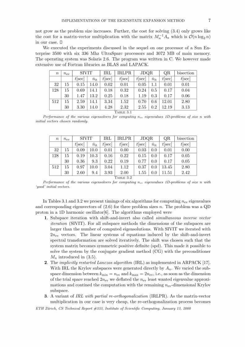
30 3.30 14.0 4.28 2.32 2.55 0.2 12.19 3.13Table 3.1

Performance of the various eigensolvers for computing nev eigenvalues 1D-problems of size n withinitial vectors chosen randomly.

n nev SIVIT IRL IRLPR JDQR QR bisectiont[sec] nit t[sec] t[sec] t[sec] nit t[sec] t[sec]

32 15 0.09 10.0 0.01 0.00 0.03 0.0 0.01 0.00128 15 0.19 10.3 0.16 0.22 0.15 0.0 0.17 0.05

30 0.36 9.3 0.22 0.19 0.77 0.0 0.17 0.05512 15 0.97 10.0 3.04 1.12 0.37 0.0 13.45 2.80

30 2.60 9.4 3.93 2.00 1.55 0.0 11.51 2.42Table 3.2

Performance of the various eigensolvers for computing nev eigenvalues 1D-problems of size n with‘good’ initial vectors.

In Tables 3.1 and 3.2 we present timings of six algorithms for computing nev eigenvaluesand corresponding eigenvectors of (2.6) for three problem sizes n. The problem was a QDproton in a 1D harmonic oscillator[6]. The algorithms employed were

1. Subspace iteration with shift-and-invert also called simultaneous inverse vectoriteration (SIVIT). For all subspace methods the dimensions of the subspaces arelarger than the number of computed eigensolutions. With SIVIT we iterated with2nev vectors. The linear systems of equations induced by the shift-and-invertspectral transformation are solved iteratively. The shift was chosen such that thesystem matrix becomes symmetric positive definite (spd). This made it possible tosolve the system by the conjugate gradient method (CG) with the preconditionerMn introduced in (3.5).

2. The implicitly restarted Lanczos algorithm (IRL) as implemented in ARPACK [17].With IRL the Krylov subspaces were generated directly by An. We varied the sub-space dimension between kmin = nev and kmax = 2nev, i.e., as soon as the dimensionof the trial space reached 2nev we deflated the nev least wanted eigenvalue approxi-mations and contined the computation with the remaining nev-dimensional Krylovsubspace.

3. A variant of IRL with partial re-orthogonalization (IRLPR). As the matrix-vectormultiplication in our case is very cheap, the re-orthogonalization process becomes

ETH Zurich, CS Technical Report #333, Institute of Scientific Computing, January 13, 2000

8 ARBENZ, BROKER, CHINELLATO, GANDER, GEUS, AND STREBEL

the dominant computational part in an ARPACK-like implementation. To re-duce this cost, we introduced partial re-orthogonalization into IRL. Partial re-orthogonalization has been invented by Simon [22, 23, 12] to prevent at a reasonablecost the loss of orthogonality among the Krylov vectors in the Lanczos algorithm.Furthermore, we worked with much larger trial spaces than with the original IRL.Its dimension ranged from kmin = nev + 8 to kmax. Initially, kmax = 2nev + 32.This value was increased by 4 after every deflation step up to kmax = 3nev + 40.These values have been found reasonable in experiments. Of course, their optimalvalues are problem dependent.

4. The Jacobi-Davidson algorithm with shift-and-invert (JDQR). In contrast to thesituation in SIVIT, in Jacobi-Davidson algorithm the shift varies during the algo-rithm. As the system of equations that has to be solved is symmetric indefinite,we used the Conjugate Gradient Squared (CGS) method to solve it. We usedthe same preconditioner Mn as with SIVIT. As with IRL we varied the subspacedimensions between kmin = nev and kmax = 2nev.

5. The QR algorithm This is the classical algorithm to compute the complete spectraldecomposition of a full (dense) matrix [1]. It proceeds in two steps. First thematrix An is reduced to a similar tridiagonal form; then the symmetric tridiagonalQR algorithm is applied. This is the algorithm used in the original GROMOS [6]implementation.

6. Bisection. If only a part (less than 30%) of the spectrum of a full matrix isneeded it is recommended [1] to replace the symmetric tridiagonal QR algorithmby tridiagonal bisection. The reduction to tridiagonal form remains the same aswith the QR algorithm.

For all eigensolvers we used a relative error tolerance of 10−6, which is accurate enough,if compared to approximation errors resulting from other parts of the calculation. In theiterative equation solvers, the relative residual was reduced to 10−8.

The timings of Table 3.1 refer to the situation where no approximations of the searchedeigenvectors are known. Here we started the iterations with random vectors. However,the vectors were chosen to be equal in the various algorithms. For the timings of Table 3.2we started with the eigenvectors of the matrix of the previous time step. These numbersare much more relevant because in real simulations one actually has to solve a sequence ofeigenvalue problems that differ only in the diagonal matrix Vn. The columns indicated bynit give the average number of iterations needed by the linear system solver to reduce theralative residual to 10−8. The optimality of our preconditioner is justified by the smallvariance of nit. Notice that this number is very small with JDQR as only little accuracyis required in the initial phase of the algorithm. Only at the end the maximal accuracyrequirement is enforced.

The results show that for the small and medium size problems bisection is fastest. Inthese cases a considerable fraction of of the eigenpairs is requested. For the small problemsize, the difference with the ordinary QR algorithm and with IRLPR is not big, however.With the largest problem size the full matrix methods cannot compete any more due totheir O(n3) complexity. Besides their high flop count the full matrix methods also consumemuch memory. Subspace methods have lower computational cost. If only 15 eigenvaluesare desired then Jacobi-Davidson is clearly fastest. If 30 eigenpairs are desired then IRLcatches up and is even faster if good eigenvector approximations are lacking.

Notice that SIVIT exploits good starting vectors very well. It is second fastest ifonly 15 eigenpairs are computed. Also JDQR makes good use of good initial vectors.In particular the number nit of ‘inner iterations’ is very small or even negligible. JDQRETH Zurich, CS Technical Report #333, Institute of Scientific Computing, January 13, 2000

IMPLEMENTATIONS OF THE EIGENSTATE EXPANSION METHOD 9

performs best if good initial vectors are available. However, its computation time increasesby about a factor of four if nev is doubled. This is because of the many projections neededin Jacobi-Davidson. For larger nev IRLPR will be competitive.

Notice that IRL and IRLPR perform in a similar way in the medium size prob-lem. For the large problem size IRL performs poorly due to the excessive number ofre-orthogonalizations. At the same time the short execution times of IRLPR show thatpartial re-orthogonalization is effective. As the trial spaces with IRLPR are very big, re-orthogonalization is extremely expensive. The timings indicate that only a small numberof re-orthogonalizations take place.

4. The 3D problem. The Schrodinger equation (1.1) for a 3-dimensional particle ofmass m that is trapped in a cubic box is given by

Hu(x) = − ~2

2m∆u(x) + V (x)u(x) = λu(x), x ∈ G := (0, 2π)3,(4.1)

where u(x) satisfies periodic boundary conditions. We approximate u(x) as a tensorproduct of Fourier polynomials of order n, n = 2q,

u(x) =

n2X

kd=−n2

+1d=1,... ,3

ckeik·x.(4.2)

Thus

−∆u(x) =

n2X

kd=−n2

+1d=1,... ,3

|k|2ckeik·x, |k|2 = k21 + k2

2 + k23.

Solving (4.2) by collocation at the points xj = 2π/n(j1, j2, j3)T , jd = 0, . . ., n − 1, d =1, . . . , 3, yields the n3 equations

n2X

kd=−n2

+1d=1,... ,3

~

2

2m|k|2 + V (xj)− λ

!cke

ik·x, jd = 0, . . . , n− 1, d = 1, . . ., 3.(4.3)

Transformations analogous to those from (2.3) to (2.4) and from (2.5) to (2.6), respectively,lead to the matrix eigenvalue problem

Anx = (FnKnF−1n + Vn)x = λx(4.4)

where

Fn = Fn ⊗ Fn ⊗ Fn,Kn = In ⊗ In ⊗Kn + In ⊗Kn ⊗ In +Kn ⊗ In ⊗ In,Vn = diag

�V (x(0,0,0)), . . . , V (x(n−1,n−1,n−1))

�.

Vn contains the values of V (x) at the grid points xi,j,k that are arranged in lexicographicorder. Setting Hn = FnKnF

−1n as in (2.6) we can write

Hn = FnKnF−1n = In ⊗ In ⊗Hn + In ⊗Hn ⊗ In +Hn ⊗ In ⊗ In.(4.5)

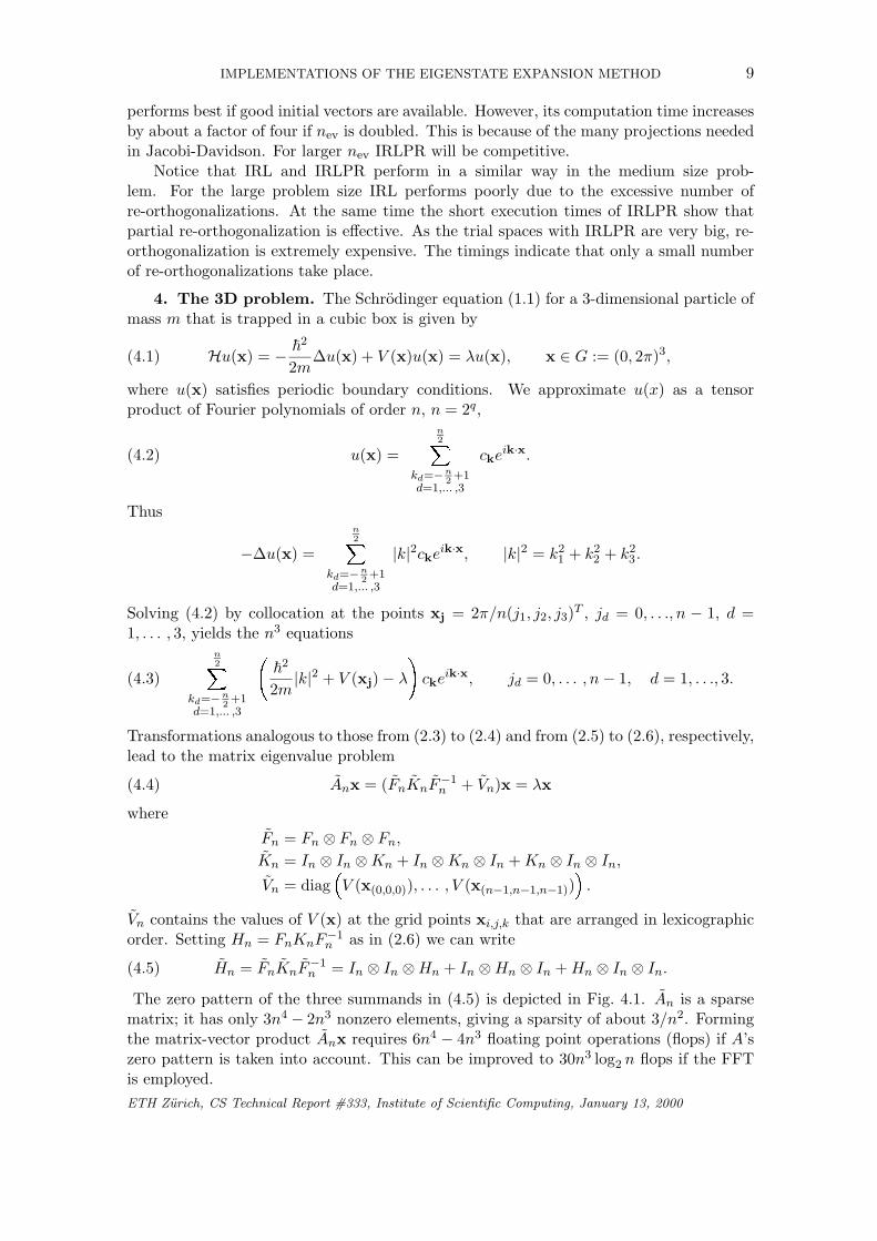
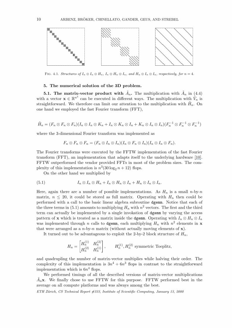
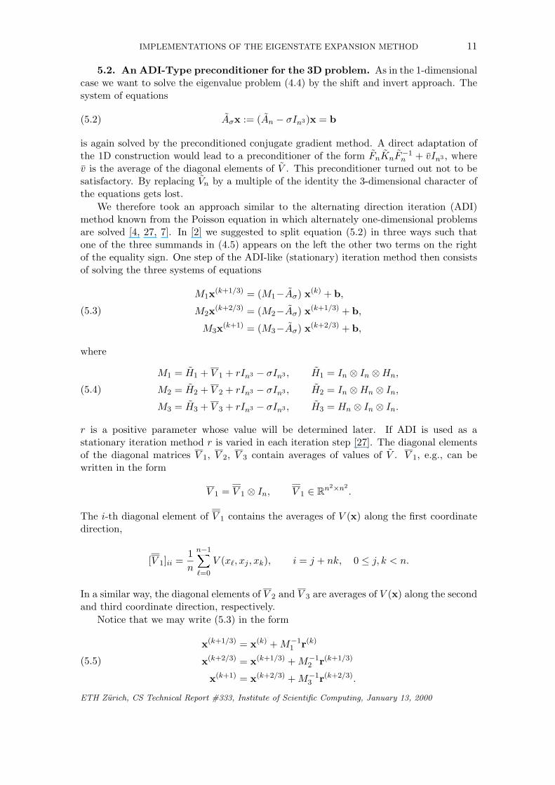
The zero pattern of the three summands in (4.5) is depicted in Fig. 4.1. An is a sparsematrix; it has only 3n4 − 2n3 nonzero elements, giving a sparsity of about 3/n2. Formingthe matrix-vector product Anx requires 6n4 − 4n3 floating point operations (flops) if A’szero pattern is taken into account. This can be improved to 30n3 log2 n flops if the FFTis employed.ETH Zurich, CS Technical Report #333, Institute of Scientific Computing, January 13, 2000

10 ARBENZ, BROKER, CHINELLATO, GANDER, GEUS, AND STREBEL

Fig. 4.1. Structures of In ⊗ In ⊗Hn, In ⊗Hn ⊗ In, and Hn ⊗ In ⊗ In, respectively, for n = 4.

5. The numerical solution of the 3D problem.

5.1. The matrix-vector product with An. The multiplication with An in (4.4)with a vector x ∈ Rn3

can be executed in different ways. The multiplication with Vn isstraightforward. We therefore can limit our attention to the multiplication with Hn. Onone hand we employed the fast Fourier transform (FFT),

Hn = (Fn ⊗ Fn ⊗ Fn)(In ⊗ In ⊗Kn + In ⊗Kn ⊗ In +Kn ⊗ In ⊗ In)(F−1n ⊗ F−1

n ⊗ F−1n )

where the 3-dimensional Fourier transform was implemented as

Fn ⊗ Fn ⊗ Fn = (Fn ⊗ In ⊗ In)(In ⊗ Fn ⊗ In)(In ⊗ In ⊗ Fn).

The Fourier transforms were executed by the FFTW implementation of the fast Fouriertransform (FFT), an implementation that adapts itself to the underlying hardware [10].FFTW outperformed the vendor provided FFTs in most of the problem sizes. The com-plexity of this implementation is n3(30 log2 n+ 12) flops.

On the other hand we multiplied by

In ⊗ In ⊗Hn + In ⊗Hn ⊗ In +Hn ⊗ In ⊗ In.(5.1)

Here, again there are a number of possible implementations. As Hn is a small n-by-nmatrix, n ≤ 20, it could be stored as full matrix. Operating with Hn then could beperformed with a call to the basic linear algebra subroutine dgemm. Notice that each ofthe three terms in (5.1) amounts to multiplying Hn with n2 vectors. The first and the thirdterm can actually be implemented by a single invokation of dgemm by varying the accesspattern of x which is treated as a matrix inside the dgemm. Operating with In ⊗Hn ⊗ Inwas implemented through n calls to dgemm, each multiplying Hn with n2 elements in xthat were arranged as a n-by-n matrix (without actually moving elements of x).

It turned out to be advantageous to exploit the 2-by-2 block structure of Hn,

Hn =

"H

(1)n H

(2)n

H(2)n H

(1)n

#, H(1)

n ,H(2)n symmetric Toeplitz,

and quadrupling the number of matrix-vector multiplies while halving their order. Thecomplexity of this implementation is 3n4 + 6n3 flops in contrast to the straightforwardimplementation which is 6n4 flops.

We performed timings of all the described versions of matrix-vector multiplicationsAnx. We finally chose to use FFTW for this purpose. FFTW performed best in theaverage on all compute platforms and was always among the best.ETH Zurich, CS Technical Report #333, Institute of Scientific Computing, January 13, 2000

IMPLEMENTATIONS OF THE EIGENSTATE EXPANSION METHOD 11

5.2. An ADI-Type preconditioner for the 3D problem. As in the 1-dimensionalcase we want to solve the eigenvalue problem (4.4) by the shift and invert approach. Thesystem of equations

Aσx := (An − σIn3)x = b(5.2)

is again solved by the preconditioned conjugate gradient method. A direct adaptation ofthe 1D construction would lead to a preconditioner of the form FnKnF

−1n + vIn3 , where

v is the average of the diagonal elements of V . This preconditioner turned out not to besatisfactory. By replacing Vn by a multiple of the identity the 3-dimensional character ofthe equations gets lost.

We therefore took an approach similar to the alternating direction iteration (ADI)method known from the Poisson equation in which alternately one-dimensional problemsare solved [4, 27, 7]. In [2] we suggested to split equation (5.2) in three ways such thatone of the three summands in (4.5) appears on the left the other two terms on the rightof the equality sign. One step of the ADI-like (stationary) iteration method then consistsof solving the three systems of equations

M1x(k+1/3) = (M1−Aσ) x(k) + b,

M2x(k+2/3) = (M2−Aσ) x(k+1/3) + b,

M3x(k+1) = (M3−Aσ) x(k+2/3) + b,

(5.3)

where

M1 = H1 + V 1 + rIn3 − σIn3 , H1 = In ⊗ In ⊗Hn,

M2 = H2 + V 2 + rIn3 − σIn3 , H2 = In ⊗Hn ⊗ In,M3 = H3 + V 3 + rIn3 − σIn3 , H3 = Hn ⊗ In ⊗ In.

(5.4)

r is a positive parameter whose value will be determined later. If ADI is used as astationary iteration method r is varied in each iteration step [27]. The diagonal elementsof the diagonal matrices V 1, V 2, V 3 contain averages of values of V . V 1, e.g., can bewritten in the form

V 1 = V 1 ⊗ In, V 1 ∈ Rn2×n2

.

The i-th diagonal element of V 1 contains the averages of V (x) along the first coordinatedirection,

[V 1]ii =1n

n−1X`=0

V (x`, xj , xk), i = j + nk, 0 ≤ j, k < n.

In a similar way, the diagonal elements of V 2 and V 3 are averages of V (x) along the secondand third coordinate direction, respectively.

Notice that we may write (5.3) in the form

x(k+1/3) = x(k) +M−11 r(k)

x(k+2/3) = x(k+1/3) +M−12 r(k+1/3)

x(k+1) = x(k+2/3) +M−13 r(k+2/3).

(5.5)

ETH Zurich, CS Technical Report #333, Institute of Scientific Computing, January 13, 2000

12 ARBENZ, BROKER, CHINELLATO, GANDER, GEUS, AND STREBEL

with r(m) := b−Aσx(m) being the residual in x(m). Each of the three systems of equationsconsists of n2 independent systems of equations of order n that differ only in the diagonal.They can be solved in parallel.

The ADI-like iteration (5.5) can be collected in one equation,

x(k+1) = x(k) +�I − (I −M−1

3 Aσ)(I −M−12 Aσ)(I −M−1

1 Aσ)�A−1σ r(k).

As the Mi do not commute, the matrix that is multiplied with r(k) is not symmetricpositive definite. Therefore, it is not suited right-away as a preconditioner for the conjugategradient method. We can however premultiply it with its transpose (adjoint) to get anadmissible (symmetric positive definite) preconditioner [4, p.289],

x(k+1/6) = x(k) +M−11 r(k)

x(k+3/6) = x(k+2/6) +M−13 r(k+2/6)

x(k+5/6) = x(k+4/6) +M−12 r(k+4/6)

x(k+2/6) = x(k+1/6) +M−12 r(k+1/6)

x(k+4/6) = x(k+3/6) +M−13 r(k+3/6)

x(k+1) = x(k+5/6) +M−11 r(k+5/6)

(5.6)

or

x(k+1) = x(k) +�I − (I −M−1

1 Aσ)(I −M−12 Aσ)(I −M−1

3 Aσ) ·

· (I −M−13 Aσ)(I −M−1

2 Aσ)(I −M−11 Aσ)

�A−1σ r(k)

=: x(k) +M−1r(k).

(5.7)

M−1 can alternatively be written in the form

M−1 = A−1σ − A−1/2

σ (I − A1/2σ M−1

1 A1/2σ )(I − A1/2

σ M−12 A1/2

σ )(I − A1/2σ M−1

3 A1/2σ ) ·

· (I − A1/2σ M−1

3 A1/2σ )(I − A1/2

σ M−12 A1/2

σ )(I − A1/2σ M−1

1 A1/2σ )

�A−1/2σ

(5.8)

The thus defined M−1 (or M) is evidently symmetric. We use this matrix as a precon-ditioner for the conjugate gradient method in the following way when solving the secondequation in (3.6). We solve Aσζ = rk approximatively by one step of the ADI-like itera-tion (5.6). The initial vector is ζ(0) = 0 and z(k) = ζ(1).

Remark 2. A different symmetric preconditioner is obtained if M−13 in (5.6) is applied

only once. This symmetrizing technique is known from overlapping Schwarz precondition-ing [25, p.14]. This preconditioner has of only five substeps,

M−1 = A−1σ − A−1/2

σ (I − A1/2σ M−1

1 A1/2σ )(I − A1/2

σ M−12 A1/2

σ )(I − A1/2σ M−1

3 A1/2σ ) ·

· (I − A1/2σ M−1

2 A1/2σ )(I − A1/2

σ M−11 A1/2

σ )�A−1/2σ .

(5.9)

One application of (5.9) is slightly cheaper than one application of the original precondi-tioner in (5.8).

Remark 3. Notice that we are free in how we select the sequence in which we go‘through the dimensions’. Here, we chose the natural sequence 1-2-3 as there is formallyno distinguished direction in the potential V (x). In practice however the selection of thesequence can be crucial for the performance of the preconditioner.

To investigate the convergence behaviour of the preconditioned conjugate gradientalgorithm we estimate the generalized condition number of M−1Aσ. As the eigenvalueproblems Aσx = λMx and M−1z = λA−1

σ z are similar, the inclusion (3.8) also holds forthe Rayleigh quotient of the latter eigenvalue problem,

0 < λ1 ≤ ρ′(z) :=z∗M−1zz∗A−1

σ z≤ λn, z 6= 0,

ETH Zurich, CS Technical Report #333, Institute of Scientific Computing, January 13, 2000

IMPLEMENTATIONS OF THE EIGENSTATE EXPANSION METHOD 13

which implies κ ≤ λn/λ1. According to (5.8) we rewrite ρ′(z) as

ρ′(z) = 1− y∗(I−A12σM

−11 A

12σ )(I−A

12σM

−12 A

12σ )(I−A

12σM

−13 A

12σ )2(I−A

12σM

−12 A

12σ )(I−A

12σM

−11 A

12σ )y

y∗y

= 1− y∗(I−A12σM

−11 A

12σ )2y

y∗yy∗1(I−A

12σM

−12 A

12σ )2y1

y∗1y1

y∗2(I−A12σM

−13 A

12σ )2y2

y∗2y2

(5.10)

where

y = A−1/2σ z, y1 = (I−A1/2

σ M−11 A1/2

σ )y,

y2 = (I−A1/2σ M−1

2 A1/2σ )y1 = (I−A1/2

σ M−12 A1/2

σ )(I−A1/2σ M−1

1 A1/2σ )y.

Clearly, ρ′(z) ≤ 1. We want to show that ρ′(z) is bounded away from zero. We do thisby treating the three quotients in (5.10) individually showing that for sufficiently large rthere are numbers bλ1(r), bλ2(r), bλ3(r) such that

ρi(y) :=y∗(I−A1/2

σ M−1i A

1/2σ )2y

y∗y≤ bλi(r) < 1, ∀y 6= 0, i = 1, 2, 3.

Then, we get

0 < 1− bλ1(r)bλ2(r)bλ3(r) ≤ ρ′(z) ≤ 1.(5.11)

Of course, we would like the above lower bound to be as large as possible. To investigatethe three individual Rayleigh quotients we can w.l.o.g. let i = 1. ρ1(y) is the Rayleighquotient of the eigenvalue problem

(I−A1/2σ M−1

1 A1/2σ )2y = A1/2

σ (I−M−11 Aσ)2A−1/2

σ y = λy.(5.12)

By substituting z = A−1/2σ y we get the eigenvalue problem

(I−M−11 Aσ)2z = λz(5.13)

which has the same eigenvalues as (5.12). The eigenvalues of (5.13) are the squares of theeigenvalues of

(I−M−11 Aσ)z = µz(5.14)

or, equivalently, of

(M1 − Aσ)z = µM1z.(5.15)

The Rayleigh quotient corresponding to (5.15) is

z∗(M1 − Aσ)zz∗M1z

.(5.16)

To improve the quality of the estimates we consider as in the 1D case the subspacesspan{1}, 1 = (1, . . . , 1)∗, and its orthogonal complement separately.

Let first x = 1. 1 is in the null space of all the Hi and further, as in one dimension,1∗(V − V 1)1 = 0. As V 1 − σI is positive definite, we get

1∗M11 = (r + v − σ)‖1‖22, v =n3Xi=1

Vii =n3Xi=1

(V 1)ii,

ETH Zurich, CS Technical Report #333, Institute of Scientific Computing, January 13, 2000

14 ARBENZ, BROKER, CHINELLATO, GANDER, GEUS, AND STREBEL

and

1∗(M1 − Aσ)11∗M11

=r

r + v − σ.(5.17)

Now let x∗1 = 0. With the notation of (5.4) we have

x∗(M1 − Aσ)xx∗M1x

=x∗(H1 + V 1 + (r − σ)I −H1 −H2 −H3 − V + σI)x

x∗(H1 + V 1 + (r − σ)I)x

=x∗(rI −H2 −H3 + (V 1 − V ))x

x∗(rI +H1 + (V 1 − σI))x

≤ x∗(rI − 2k1 + (V 1 − V ))xx∗(rI + k1 + (V 1 − σI))x

= maxi

r − 2k1 + ((V 1)ii − Vii)r + k1 + (V 1)ii − σ

=: bµ1(r).

(5.18)

and

x∗(rI −H2 −H3 + (V 1 − V ))xx∗(rI +H1 + (V 1 − σI))x

≥ x∗(rI − 2kn + (V 1 − V ))xx∗(rI + k1 + (V 1 − σI))x

= mini

r − 2kn + ((V 1)ii − Vii)r + k1 + (V 1)ii − σ

=: eµ1(r).(5.19)

Both upper bound bµ1(r) and lower bound eµ1(r) increase with r and converge to 1 frombelow as r tends to infinity. bµ1 is positive for r > 2k1 and less than 1. eµ1 is negativefor r = 0. If r is chosen so big that the lower bound is above −1 then the eigenvaluesof (5.13) are bounded by bλ1(r) = µi(r)2 := max{|eµi(r)|, bµi(r)}2 < 1. In a similar way wecan bound ρ2(z) and ρ3(z).

By construction, eµi(r) < bµi(r). In particular, if r > ri where −eµi(ri) = bµi(ri), then|eµi(r)| ≤ bµi(r). If such an ri does not exist we set ri = 0. From (5.18) we see that bµi(ri)does not depend on n.

If we set r0 := max{r1, r2, r3}, then we haveTheorem 5.1. Let σ = minV (xj) and let M = M(r0). The generalized condition

number κ(Aσ,M) is bounded independently of the problem size,

κ = κM(r0)(M(r0)−1Aσ) ≤ 11− bµ1(r0)2bµ2(r0)2bµ3(r0)2

(5.20)

where r0 := max{r1, r2, r3} and the ri are defined by

ri := max{0, {r > 0| − eµi(r) = bµi(r)}}.Remark 4. A better bound than in (5.20) may be obtained if the function

3Yi=1

µi(r)2, µi(r) := max{|eµi(r)|, bµi(r)}.

is directly minimized for r ≥ 0.ETH Zurich, CS Technical Report #333, Institute of Scientific Computing, January 13, 2000

IMPLEMENTATIONS OF THE EIGENSTATE EXPANSION METHOD 15

We now turn to the alternative preconditioner (5.9). Instead of the Rayleigh quotientin (5.10) we have to deal with

ρ′′(z) =y∗(I−A

12σM

−11 A

12σ )2y

y∗y| {z }ρ1(y)

y∗1(I−A12σM

−12 A

12σ )2y1

y∗1y1| {z }ρ2(y1)

y∗2(I−A12σM

−13 A

12σ )y2

y∗2y2| {z }ρ′′3(y2)

(5.21)

The estimates for ρ1(y) and ρ2(y1) carry over from (5.18)-(5.19). ρ′′3(y2) is up to a changeof variables the Rayleigh quotient given in (5.16) with M1 replaced by M3. Hence,

1− µ1(r)2µ2(r)2bµ3(r) ≤ ρ′′3(z) ≤ 1− µ1(r)2µ2(r)2eµ3(r).

Notice that eµ3(r) may be negative. In fact this is the interesting situation. If eµ3(r) forsome reason approches -1 only very slowly then the r0 in Theorem 5.1 will be very large.This means that the µi(r) are all very close to 1 implying a high condition number κ. Ifwe can choose r0 much smaller, eµ3(r) may still be below -1, but 1− µ1(r)2µ2(r)2bµ3(r) ismuch further away from 0 leading to a much better condition number. We formulate

Theorem 5.2. The condition number

κ ≤ 1− µ1(r)2µ2(r)2eµ3(r)1− µ1(r)2µ2(r)2bµ3(r)

(5.22)

depends “slightly” on the problem size n as the numerator in (5.22) contains the term~

2

2m

�n2

�2.

5.3. Numerical experiments. In this section we report on experiments with a re-alistic example from mixed QM/CM simulation [6]. There is a single quantum particle,an excess proton, immersed in fluid water (at 300 K) modeled by 216 water molecules.The proton state is modeled by a tensor product of three Fourier polynomials of degreen, cf. (4.2). In our examples n takes on the values 12, 16, and 18, giving rise to matrixorders N = n3 = 1728, 4096, and 5832, respectively. The computations were performedon the same compute platform as the 1D problems, Sun Enterprise 3500. For details seesection 3.

We computed the 15 and 30, respectively, smallest eigenvalues and correspondingeigenvectors with the methods that we found the most promising from the 1D experiments,subspace iteration (SIVIT), the Jacobi-Davidson (JDQR) algorithm, and the implicitlyrestarted Lanczos algorithm with partial re-orthogonalization.

Table 5.1 shows the timings for eigensolvers when started with randomly chosen start-ing vectors. Table 5.2 shows the timings for solving (almost) the same problems withinitial vectors that are the eigenvectors of the eigenvalue problem of the previous timestep. The execution times t are given in seconds. ncg is the number of times the (precon-ditioned) conjugate gradient algorithm was invoked. With SIVIT, this happens 2nev timesin each update of the trial space. The columns indicated by nit give the average numberof iterations of pcg until convergence. Notice, that in JDQR the error tolerance in theconjugate gradient method varies. Being loose initially, the error tolerance is tightened ineach inner iteration [3, 9]. Therefore, the number of iterations until convergence of cg isnot constant. We only list timings with an ADI-like preconditioners of type (5.9). Thesubscripts in ADI13231 indicate the sequence in which the Gi have been applied. We setthe parameter r=500, a value that was found through experiments. The results reportedin [2] show that the preconditioners of the form (5.8) do not perform as well as those of theform (5.9), whence they are omitted here. In IRLPR there are no systems of equations toETH Zurich, CS Technical Report #333, Institute of Scientific Computing, January 13, 2000

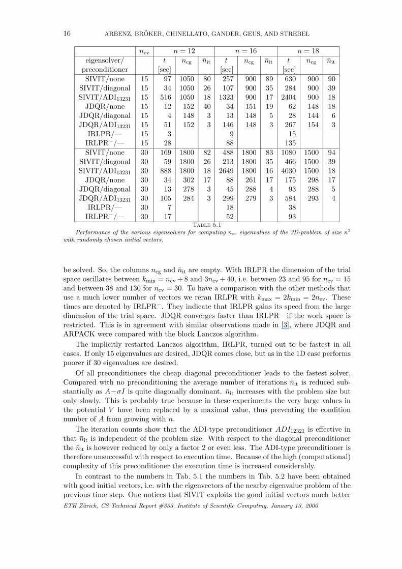
16 ARBENZ, BROKER, CHINELLATO, GANDER, GEUS, AND STREBEL

nev n = 12 n = 16 n = 18eigensolver/ t ncg nit t ncg nit t ncg nit

preconditioner [sec] [sec] [sec]SIVIT/none 15 97 1050 80 257 900 89 630 900 90

SIVIT/diagonal 15 34 1050 26 107 900 35 284 900 39SIVIT/ADI13231 15 516 1050 18 1323 900 17 2404 900 18

JDQR/none 15 12 152 40 34 151 19 62 148 18JDQR/diagonal 15 4 148 3 13 148 5 28 144 6JDQR/ADI13231 15 51 152 3 146 148 3 267 154 3

IRLPR/— 15 3 9 15IRLPR−/— 15 28 88 135SIVIT/none 30 169 1800 82 488 1800 83 1080 1500 94

SIVIT/diagonal 30 59 1800 26 213 1800 35 466 1500 39SIVIT/ADI13231 30 888 1800 18 2649 1800 16 4030 1500 18

JDQR/none 30 34 302 17 88 261 17 175 298 17JDQR/diagonal 30 13 278 3 45 288 4 93 288 5JDQR/ADI13231 30 105 284 3 299 279 3 584 293 4

IRLPR/— 30 7 18 38IRLPR−/— 30 17 52 93

Table 5.1

Performance of the various eigensolvers for computing nev eigenvalues of the 3D-problem of size n3

with randomly chosen initial vectors.

be solved. So, the columns ncg and nit are empty. With IRLPR the dimension of the trialspace oscillates between kmin = nev + 8 and 3nev + 40, i.e. between 23 and 95 for nev = 15and between 38 and 130 for nev = 30. To have a comparison with the other methods thatuse a much lower number of vectors we reran IRLPR with kmax = 2kmin = 2nev. Thesetimes are denoted by IRLPR−. They indicate that IRLPR gains its speed from the largedimension of the trial space. JDQR converges faster than IRLPR− if the work space isrestricted. This is in agreement with similar observations made in [3], where JDQR andARPACK were compared with the block Lanczos algorithm.

The implicitly restarted Lanczos algorithm, IRLPR, turned out to be fastest in allcases. If only 15 eigenvalues are desired, JDQR comes close, but as in the 1D case performspoorer if 30 eigenvalues are desired.

Of all preconditioners the cheap diagonal preconditioner leads to the fastest solver.Compared with no preconditioning the average number of iterations nit is reduced sub-stantially as A−σI is quite diagonally dominant. nit increases with the problem size butonly slowly. This is probably true because in these experiments the very large values inthe potential V have been replaced by a maximal value, thus preventing the conditionnumber of A from growing with n.

The iteration counts show that the ADI-type preconditioner ADI12321 is effective inthat nit is independent of the problem size. With respect to the diagonal preconditionerthe nit is however reduced by only a factor 2 or even less. The ADI-type preconditioner istherefore unsuccessful with respect to execution time. Because of the high (computational)complexity of this preconditioner the execution time is increased considerably.

In contrast to the numbers in Tab. 5.1 the numbers in Tab. 5.2 have been obtainedwith good initial vectors, i.e. with the eigenvectors of the nearby eigenvalue problem of theprevious time step. One notices that SIVIT exploits the good initial vectors much betterETH Zurich, CS Technical Report #333, Institute of Scientific Computing, January 13, 2000

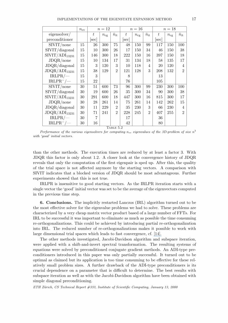
IMPLEMENTATIONS OF THE EIGENSTATE EXPANSION METHOD 17

nev n = 12 n = 16 n = 18eigensolver/ t ncg nit t ncg nit t ncg nit

preconditioner [sec] [sec] [sec]SIVIT/none 15 26 300 75 48 150 99 117 150 100

SIVIT/diagonal 15 10 300 26 17 150 34 46 150 38SIVIT/ADI13231 15 146 300 18 222 150 16 397 150 18

JDQR/none 15 10 134 17 31 134 18 58 135 17JDQR/diagonal 15 3 120 3 10 118 4 20 120 4JDQR/ADI13231 15 38 129 2 121 128 3 208 132 2

IRLPR/— 15 3 8 13IRLPR−/— 15 22 76 105SIVIT/none 30 51 600 73 96 300 99 230 300 100

SIVIT/diagonal 30 19 600 26 35 300 34 90 300 38SIVIT/ADI13231 30 291 600 18 447 300 16 815 300 17

JDQR/none 30 28 261 14 75 261 14 142 262 15JDQR/diagonal 30 11 229 2 35 230 3 66 230 4JDQR/ADI13231 30 71 241 2 228 245 2 407 255 2

IRLPR/— 30 7 17 36IRLPR−/— 30 16 42 80

Table 5.2

Performance of the various eigensolvers for computing nev eigenvalues of the 3D-problem of size n3

with ‘good’ initial vectors.

than the other methods. The execution times are reduced by at least a factor 3. WithJDQR this factor is only about 1.2. A closer look at the convergence history of JDQRreveals that only the computation of the first eigenpair is sped up. After this, the qualityof the trial space is not affected anymore by the starting vectors. A comparison withSIVIT indicates that a blocked version of JDQR should be most advantageous. Furtherexperiments showed that this is not true.

IRLPR is insensitive to good starting vectors. As the IRLPR iteration starts with asingle vector the ‘good’ initial vector was set to be the average of the eigenvectors computedin the previous time step.

6. Conclusions. The implicitly restarted Lanczos (IRL) algorithm turned out to bethe most effective solver for the eigenvalue problems we had to solve. These problems arecharacterized by a very cheap matrix vector product based of a large number of FFTs. ForIRL to be successful it was important to eliminate as much as possible the time consumingre-orthogonalizations. This could be achieved by introducing partial re-orthogonalizationinto IRL. The reduced number of re-orthogonalizations makes it possible to work withlarge dimensional trial spaces which leads to fast convergence, cf. [14].

The other methods investigated, Jacobi-Davidson algorithm and subspace iteration,were applied with a shift-and-invert spectral transformation. The resulting systems ofequations were solved by preconditioned conjugate gradient methods. An ADI-type pre-conditioners introduced in this paper was only partially successful. It turned out to beoptimal as claimed but its application is too time consuming to be effective for these rel-atively small problem sizes. A further drawback of the ADI-type preconditioners is itscrucial dependence on a parameter that is difficult to determine. The best results withsubspace iteration as well as with the Jacobi-Davidson algorithm have been obtained withsimple diagonal preconditioning.ETH Zurich, CS Technical Report #333, Institute of Scientific Computing, January 13, 2000

18 ARBENZ, BROKER, CHINELLATO, GANDER, GEUS, AND STREBEL

The problem at hand is best solved with our implementation of the implicitly restartedLanczos algorithm provided that there is enough memory space available to increase thedimension of the trial space to three or even four times the number of eigenvalues desired.Jacobi-Davidson is to be preferred to the implicitly restarted Lanczos algorithm if theworkspace is limited and only few vectors can be stored besides the eigenvectors that areto be computed.

REFERENCES

[1] E. Anderson, Z. Bai, C. Bischof, J. Demmel, J. Dongarra, J. D. Croz, A. Greenbaum,

S. Hammarling, A. McKenney, S. Ostrouchov, and D. Sorensen, LAPACK Users’ Guide- Release 2.0, Society for Industrial and Applied Mathematics, Philadelphia, PA, 1994. (Softwareand guide are available from Netlib at URL http://www.netlib.org/lapack/).

[2] P. Arbenz, Towards an efficient implementation of the eigenstate expansion method for quan-tum molecular dynamics simulations, in 2nd Workshop on Large-Scale Scientific Computations,S. Margenov, P. Vassilevski, and P. Yalamov, eds., Vieweg, Braunschweig, 2000.

[3] P. Arbenz and R. Geus, A comparison of solvers for large eigenvalue problems originating fromMaxwell’s equations, Numer. Lin. Alg. Appl., 6 (1999), pp. 3–16.

[4] O. Axelsson, Iterative Solution Methods, Cambridge University Press, Cambridge, 1994.[5] S. R. Billeter and W. F. van Gunsteren, A comparison of different numerical propagation

schemes for solving the time-dependent Schrodinger equation in the position representation inone dimension for mixed quantum- and molecular dynamics simulations, Mol. Sim., 15 (1995),pp. 301–322.

[6] , A modular molecular dynamics / quantum dynamics program for non-adiabatic proton trans-fers in solution, Comput. Phys. Comm., 107 (1997), pp. 61–91.

[7] P. Concus and G. H. Golub, Use of fast direct methods for the efficient numerical solution ofnonseparable elliptic equations, SIAM J. Numer. Anal., 10 (1973), pp. 1103–1120.

[8] T. Ericsson, Implementation and applications of the spectral transformation Lanczos algorithm, inMatrix Pencils, B. Kagstrom and A. Ruhe, eds., Berlin, 1983, Springer, pp. 177–188. (LectureNotes in Mathematics, 973).

[9] D. R. Fokkema, G. L. G. Sleijpen, and H. A. van der Vorst, Jacobi-Davidson style QR andQZ algorithms for the partial reduction of matrix pencils, SIAM J. Sci. Comput., 20 (1998),pp. 94–125.

[10] M. Frigo and S. G. Johnson, FFTW: An adaptive software architecture for the FFT, in Pro-ceedings of the 1998 IEEE International Conference on Acoustics, Speech and Signal Processing(ICASSP ’98), vol. 3, IEEE Service Center, Piscataway, NJ, 1998, pp. 1381–1384. (Available atURL http://www.fftw.org).

[11] A. Greenbaum, Iterative Methods for Solving Linear Systems, SIAM, Philadelphia, PA, 1997.[12] R. Grimes, J. G. Lewis, and H. Simon, A shifted block Lanczos algorithm for solving sparse

symmetric generalized eigenproblems, SIAM J. Matrix Anal. Appl., 15 (1994), pp. 228–272.[13] W. F. van Gunsteren, S. R. Billeter, A. A. Eising, P. H. Hunenberger, P. Kruger, A. E.

Mark, W. R. P. Scott, and I. G. Tironi, Biomolecular Simulation: The GROMOS96 Man-ual and User Guide, Vdf Hochschulverlag, ETH Zurich, 1996. (Information available at URLhttp://igc.ethz.ch/gromos/).

[14] M. Hochbruck and C. Lubich, On Krylov subspace approximations to the matrix exponentialoperator, SIAM J. Numer. Anal., 34 (1997), pp. 1911–1925.

[15] R. A. Horn and C. R. Johnson, Topics in Matrix Analysis, Cambridge University Press, Cam-bridge, 1991.

[16] D. J. Kouri and D. K. Hoffman, Toward a new time-dependent path integral formalism based onrestricted quantum propagators for physically realizable systems, Journal of Physical Chemistry,96 (1992), pp. 9631–9636.

[17] R. B. Lehoucq, D. C. Sorensen, and C. Yang, ARPACK Users’ Guide: Solu-tion of Large-Scale Eigenvalue Problems by Implicitely Restarted Arnoldi Methods, SIAM,Philadelphia, PA, 1998. (The software and this manual are available at URLhttp://www.caam.rice.edu/software/ARPACK/).

[18] C. van Loan, Computational Frameworks for the Fast Fourier Transform, Society for Industrial andApplied Mathematics, Philadelphia, PA, 1992. (Frontiers in applied mathematics, 10).

[19] B. Nour-Omid, B. N. Parlett, T. Ericsson, and P. S. Jensen, How to implement the spectraltransformation, Math. Comp., 48 (1987), pp. 663–673.

ETH Zurich, CS Technical Report #333, Institute of Scientific Computing, January 13, 2000

IMPLEMENTATIONS OF THE EIGENSTATE EXPANSION METHOD 19

[20] B. N. Parlett, The Symmetric Eigenvalue Problem, Prentice Hall, Englewood Cliffs, NJ, 1980.(Republished by SIAM, Philadelphia, 1998.).

[21] D. S. Scott, The advantages of inverted operators in Rayleigh-Ritz approximations, SIAM J. Sci.Stat. Comput., 3 (1982), pp. 68–75.

[22] H. Simon, Analysis of the symmetric Lanczos algorithm with reorthogonalization methods, LinearAlgebra Appl., 61 (1984), pp. 101–132.

[23] , The Lanczos algorithm with partial reorthogonalization, Math. Comp., 42 (1984), pp. 115–142.[24] G. L. G. Sleijpen and H. A. van der Vorst, A Jacobi-Davidson iteration method for linear

eigenvalue problems, SIAM J. Matrix Anal. Appl., 17 (1995), pp. 401–425.[25] B. F. Smith, P. E. Bjørstad, and W. D. Gropp, Domain Decomposition: Parallel Multilevel Meth-

ods for Elliptic Partial Differential Equations, Cambridge University Press, Cambridge, 1996.[26] J. Stoer, Einfuhrung in die Numerische Mathematik I, Springer-Verlag, Berlin, 4th ed., 1983.[27] J. Stoer and R. Bulirsch, Einfuhrung in die Numerische Mathematik II, Springer-Verlag, Berlin,

2nd ed., 1978.

ETH Zurich, CS Technical Report #333, Institute of Scientific Computing, January 13, 2000