A comparison of multiple indicator kriging and area-to-point Poisson kriging for mapping patterns of...

This article was downloaded by: [Ruth Kerry]On: 20 March 2012, At: 11:51Publisher: Taylor & FrancisInforma Ltd Registered in England and Wales Registered Number: 1072954 Registeredoffice: Mortimer House, 37-41 Mortimer Street, London W1T 3JH, UK

International Journal of GeographicalInformation SciencePublication details, including instructions for authors andsubscription information:http://www.tandfonline.com/loi/tgis20

A comparison of multiple indicatorkriging and area-to-point Poissonkriging for mapping patterns ofherbivore species abundance in KrugerNational Park, South AfricaRuth Kerry a , Pierre Goovaerts b , Izak P.J. Smit c & Ben R. Ingramd

a Department of Geography, Brigham Young University, Provo, UT,USAb Biomedware Inc., Ann Arbor, MI, USAc Scientific Services, South African National Parks, Skukuza, SouthAfricad Facultad de Ingeniería, Universidad de Talca, Curicó, Chile

Available online: 20 Mar 2012

To cite this article: Ruth Kerry, Pierre Goovaerts, Izak P.J. Smit & Ben R. Ingram (2012): Acomparison of multiple indicator kriging and area-to-point Poisson kriging for mapping patternsof herbivore species abundance in Kruger National Park, South Africa, International Journal ofGeographical Information Science, DOI:10.1080/13658816.2012.663917

To link to this article: http://dx.doi.org/10.1080/13658816.2012.663917

PLEASE SCROLL DOWN FOR ARTICLE

Full terms and conditions of use: http://www.tandfonline.com/page/terms-and-conditions

This article may be used for research, teaching, and private study purposes. Anysubstantial or systematic reproduction, redistribution, reselling, loan, sub-licensing,systematic supply, or distribution in any form to anyone is expressly forbidden.

http://www.tandfonline.com/loi/tgis20

http://dx.doi.org/10.1080/13658816.2012.663917

http://www.tandfonline.com/page/terms-and-conditions

http://www.tandfonline.com/page/terms-and-conditions

The publisher does not give any warranty express or implied or make any representationthat the contents will be complete or accurate or up to date. The accuracy of anyinstructions, formulae, and drug doses should be independently verified with primarysources. The publisher shall not be liable for any loss, actions, claims, proceedings,demand, or costs or damages whatsoever or howsoever caused arising directly orindirectly in connection with or arising out of the use of this material.

Dow

nloa

ded

by [

Rut

h K

erry

] at

11:

51 2

0 M

arch

201

2

International Journal of Geographical Information ScienceiFirst, 2012, 1–21

A comparison of multiple indicator kriging and area-to-point Poissonkriging for mapping patterns of herbivore species abundance

in Kruger National Park, South Africa

Ruth Kerrya*, Pierre Goovaertsb , Izak P.J. Smitc and Ben R. Ingramd

aDepartment of Geography, Brigham Young University, Provo, UT, USA; bBiomedware Inc., AnnArbor, MI, USA; cScientific Services, South African National Parks, Skukuza, South Africa;

dFacultad de Ingeniería, Universidad de Talca, Curicó, Chile

(Received 17 May 2011; final version received 30 January 2012)

Kruger National Park (KNP), South Africa, provides protected habitats for the uniqueanimals of the African savannah. For the past 40 years, annual aerial surveys of her-bivores have been conducted to aid management decisions based on (1) the spatialdistribution of species throughout the park and (2) total species populations in a year.The surveys are extremely time consuming and costly. For many years, the whole parkwas surveyed, but in 1998 a transect survey approach was adopted. This is cheaper andless time consuming but leaves gaps in the data spatially. Also the distance methodcurrently employed by the park only gives estimates of total species populations butnot their spatial distribution. We compare the ability of multiple indicator krigingand area-to-point Poisson kriging to accurately map species distribution in the park.A leave-one-out cross-validation approach indicates that multiple indicator krigingmakes poor estimates of the number of animals, particularly the few large counts, asthe indicator variograms for such high thresholds are pure nugget. Poisson kriging wasapplied to the prediction of two types of abundance data: spatial density and propor-tion of a given species. Both Poisson approaches had standardized mean absolute errors(St. MAEs) of animal counts at least an order of magnitude lower than multiple indi-cator kriging. The spatial density, Poisson approach (1), gave the lowest St. MAEs forthe most abundant species and the proportion, Poisson approach (2), did for the leastabundant species. Incorporating environmental data into Poisson approach (2) furtherreduced St. MAEs.

Keywords: multiple indicator kriging; area-to-point Poisson kriging; geostatistics;herbivores; Kruger National Park

1. Introduction

Kruger National Park (KNP), South Africa, provides 19,485 km2 of protected habitatsfor the unique biodiversity of the African savannah. Accurate estimation of abundanceof large herbivores in both space and time is an integral component of conservation andmanagement activities in KNP. Monitoring herbivore spatio-temporal abundance patternscan help detect and mitigate unacceptable levels of population change. Consequently,annual aerial surveys to monitor large herbivore populations have been conducted forthe last 40 years. Results from these surveys have, inter alia, been used to understand

*Corresponding author. Email: [email protected]

ISSN 1365-8816 print/ISSN 1362-3087 online© 2012 Taylor & Francishttp://dx.doi.org/10.1080/13658816.2012.663917http://www.tandfonline.com

Dow

nloa

ded

by [

Rut

h K

erry

] at

11:

51 2

0 M

arch

201

2

2 R. Kerry et al.

(1) herbivore distribution patterns in relation to resources (e.g. Smit 2011), (2) howdynamic environmental factors influence herbivore population trends (e.g. Ogutu andOwen-Smith 2003, Owen-Smith and Mills 2006), (3) population declines and possible rea-sons therefore (Harrington et al. 1999, Kshatriya et al. 2001) and (4) how past managementactions and possible future scenarios have or may influence herbivore distribution patterns(e.g. Smit and Grant 2009, Smit and Ferreira 2010).

From 1980 to 1993, the whole park was surveyed annually, but this was costly andtime consuming. It involved almost 4 months of near-constant flying with four observerson board. In 1998, the park-wide census approach was replaced by a sampling strategywhereby the number of animals is recorded along 800 m wide East–West transects, spacedat intervals of 2.5–5.6 km (Kruger et al. 2008). However, such strip transects leave ‘gaps’in the data spatially. The park currently uses a distance sampling method (Buckland et al.1993) to estimate the total number of various species in the park from the transect data.This method is based on fitting for each species a detection function based on the countdata collected in various distance bands perpendicular to the aircraft. This method can alsobe used for ground surveys (Ogutu et al. 2006). Currently, Kruger Park scientists use the‘DISTANCE’ software developed by Thomas et al. (2004) for this analysis (Kruger et al.2008).

While the distance method generates global estimates of a species population in thepark which are helpful in identifying increases or declines in population numbers, theseestimates cannot be used to fill the gaps between survey transects and produce maps ofanimal distribution in a given season. Such maps are particularly useful for understandingherbivore distribution patterns in relation to resources, how dynamic environmental factorsinfluence herbivore population trends and how management actions, such as artificial waterprovision and fire management, influence herbivore distribution patterns. In addition, espe-cially for less abundant species or species that tend to be clustered in space, the followingassumptions of the distance method are not met: (1) all animals on the transect line aredetected, (2) animals are counted accurately, (3) all animals are observed in their originallocations and (4) 60–80 sightings of each species are made per transect. Another potentialproblem with the distance method is that there seems to be a lot more noise in the totalcounts for the park when it is used (1998–2005) compared with the counts based on thefull survey of the park (1985–1993) (Figure 1b), and the associated confidence intervalsare wide. The large uncertainties and the spatial gaps associated with analysing the tran-sect data with the distance method have prohibited using the data from the past 14 years tothe same extent as the data from the previous surveys where the entire park was censused.Techniques that can (1) provide reliable interpolation results for the gaps left by the sam-pling design and (2) increase the accuracy of the population estimates will greatly increasethe value of this data set and will allow the answering of ecological and management ques-tions currently not possible. In this article, our primary aim is to determine if multipleindicator kriging or area-to-point Poisson kriging can achieve the first of these goals.

There have been several applications of geostatistics to the mapping of wildlife pop-ulations. For example, Vandermeer and Leopold (1995) used variants of kriging to assesspopulation size for the European storm petrel while Palma et al. (1999) presented an appli-cation to the Iberian lynx. At first glance, geostatistical methods seem ideal for populatingdata gaps between transects since they do not require some of the assumptions of the dis-tance method, and numerous studies have demonstrated the greater accuracy of krigingrelative to other common interpolation methods such as inverse distance, cubic splinesand classification (Voltz and Webster 1990, Gotway et al. 1996, Kravchenko and Bullock1999).

Dow

nloa

ded

by [

Rut

h K

erry

] at

11:

51 2

0 M

arch

201

2

International Journal of Geographical Information Science 3

300

(a)(b)

160,000

140,000

120,000

100,000

80,000

60,000

40,000

20,000

0

1984

1986

1988

1990

1992

1994

1996

1998

2000

2002

2004

2006

250

200

150

Fre

quency

100

50

00 20 40 60

Number of impala

80 100

Year

Impala

Whole park survey

Distance method

Poisson krigingNum

ber

of

impala

in K

NP

Figure 1. (a) Histogram of impala count observations along transects in Kruger National Park for2001 and (b) numbers of impala observed in Kruger National Park when the whole park was surveyed(1985–1993) and estimated from transects using the distance method (with 95% confidence intervals)and area-to-point Poisson kriging approach (2), 1998–2005.

Steffens (1992) completed a geostatistical study of animal count data from KNP andsuggested that should the park ever have to reduce the density of survey due to bud-get constraints, geostatistical methods would be appropriate for populating data gaps.Steffens (1992) recognized that the count data at point locations could not be directlyused for ordinary kriging and counts first had to be aggregated to blocks. Yet, he pro-ceeded to use traditional method of moments variograms and cross-variograms when thehistograms for the derived animal count data were all highly positively skewed. When dataare highly skewed or contain numerous outliers, the method of moments variogram esti-mator can be extremely unstable (Lark 2000, 2002, 2003, Kerry et al. 2007a, b, Bellieret al. 2010). This is especially the case for the rarer species or those that tend to clus-ter spatially. Rossi et al. (1992) provided a comprehensive overview of the ways in whichgeostatistical tools could be used to interpret and map patterns of spatial dependence inorganisms and the many environmental variables with which they interact. They noted thatthe traditional variogram provides an incomplete and misleading summary of these pat-terns when the local means and variances change spatially or when data contain manyoutliers. They suggested the use of indicator variograms for presence/absence data androbust variogram estimators when there are many outliers in the data. Indicator variogramshave been used to characterize variables with highly skewed histograms in several pol-lution studies (Goovaerts 1994, Goovaerts et al. 1997, Van Meirvenne and Goovaerts2001, Lin et al. 2002, Saito and Goovaerts 2002, Liu et al. 2004, Lee et al. 2007)where indicator kriging was used to estimate the probability that various critical pollu-tion thresholds are exceeded in a given location. Indicator kriging has also been usedto delineate high-density areas in spatial Poisson fields of unexploded ordnance (Saitoand McKenna 2007). Therefore, in conjunction with Rossi et al.’s (1992) recommen-dation, and the fact that animal count data are usually highly skewed, we first adoptedan indicator approach for the animal count data treating each count number as a sepa-rate threshold. The number of separate variograms that need to be computed, modelledand used in post-processing can, however, make the approach very time consuming andcomputationally intensive. To facilitate the implementation of the indicator approach with

Dow

nloa

ded

by [

Rut

h K

erry

] at

11:

51 2

0 M

arch

201

2

4 R. Kerry et al.

many thresholds, Goovaerts (2009) devised an auto-indicator kriging (Auto-IK) approachwhereby the variograms for each threshold are computed and modelled automatically, fol-lowed by multiple indicator kriging. We investigate the use of this approach here with theanimal count data.

We also explored a more recent approach to mapping count or density data that weredevised after the review paper by Rossi et al. (1992), namely Poisson kriging (Monestiezet al. 2006, Bellier et al. 2010). The positive skew in the histograms of animal count datatends to approach the Poisson distribution (Figure 1a) and thus seems more appropriatefor use with Poisson kriging than robust estimators because the latter are designed morespecifically to deal with outliers rather than underlying asymmetry. Poisson kriging wasdeveloped by Monestiez et al. (2006) to obtain accurate maps of relative abundance ofwhales in the Mediterranean Sea on the basis of spatially heterogeneous observation effortsand infrequent and sparse animal sightings. The same approach was then applied to rates ofphenomena like diseases (Goovaerts 2005) or crime (Kerry et al. 2010) where the denom-inator is a population size instead of observation time. Data based on larger populationsreceive more weight in the computation of the variogram and the kriging estimate throughthe incorporation of an ‘error variance’ term, derived from the Poisson distribution. Here,we applied the Poisson approach using two types of denominator for the KNP animal countdata: (1) size of observational areas to map the spatial density of each species and (2) totalnumber of animals from all species within areas of fixed size to map the relative propor-tion of each species. The predictions from both Poisson kriging methods were convertedto counts to allow direct comparison with the estimates from multiple indicator kriging.The change of support associated with the computation of point estimates from block data(blocks of various sizes in Poisson approach (1) and constant size in Poisson approach(2)) was accomplished using area-to-point kriging (Kyriakidis 2004). This is an importantissue that previous wildlife studies like that of Steffens (1992) did not take into account.Dealing with the change of support using area-to-point Poisson kriging allows the pro-duction of reliable maps of animal distribution patterns while also giving sensible totalpopulation estimates of each species for the park that are similar in magnitude to thoseof the distance method (see Figure 1b for an example). Area-to-point Poisson kriging,although evident in the health geography literature, has not been used in the wildlife con-text where administrative geographies with known populations are not in place, and thisrequires the development of new methods for preprocessing data.

As mentioned earlier, the main aim of this article is to compare the performanceof multiple indicator kriging and two area-to-point Poisson kriging approaches for map-ping the spatial distribution of species abundance. Multiple indicator kriging and Poissonkriging are univariate approaches as animal abundance is estimated using only the spa-tial autocorrelation among animal counts. Such spatial autocorrelation is, however, anexpected function of animal social behaviour and spatial autocorrelation in environmentalfactors which influence animal distribution. Therefore, the benefit of incorporating envi-ronmental data as secondary information into Poisson kriging approach (2) was also brieflyexplored.

2. Methods

2.1. Animal count observations

Animal counts were made during the dry season when leaves are generally absent fromtrees from a fixed-winged aircraft flying at approximately 76 m height and a speed of167–185 km h–1. A frame fitted to the aircraft (or calibrated strips drawn on the side

Dow

nloa

ded

by [

Rut

h K

erry

] at

11:

51 2

0 M

arch

201

2


windows of the aircraft) enabled animals to be located within distance classes (up to 50,100, 200 and 400 m) from the plane on either side (see Figure 2 in Kruger et al. 2008). Thismeans that observations were made along East–West running transects that were 800 mwide, but also included a 36 m invisible zone under the aircraft. Transects were spaced atvarious intervals to achieve a specified percent coverage of the park in different years. Forexample in 1998–2000, 64 transects were spaced at 5.6 km intervals to achieve 15% cov-erage of the park. The coverage of the park in other years was 22% in 2001–2003 and 22%in the south and 28% in the north in 2005–2006. Each time an animal or group of animalswas observed from the plane, the position along the transect was recorded using a GPS, aswell as the number of animals observed, the species and the distance class from the plane.No indication, however, was given of which side of the plane the animals were observed,and each species observed was recorded separately. Some potential errors associated withthese observation methods include but are not limited to

(1) miscounting/mere estimates of the count when large herds of the same species arepresent or altogether missing individuals or small herds (Redfern et al. 2002);

(2) animals under the plane are not counted;(3) counts are likely to be influenced by environmental conditions (e.g. vegetation

cover) as well as differences in cryptic colouration of animals (e.g. zebra is moreconspicuous than impala) (Redfern et al. 2002);

(4) location inaccuracies due to time delay in position recording when multiple speciesare present in one location; and

(5) animals that move from one side of the plane to the other during flight can bedouble counted.

2.2. Environmental data

Several environmental data sets were available for KNP. The continuous variables includedherbaceous biomass (B) estimated by cokriging of ground measurements of herbaceousbiomass with Advanced Very High Resolution Radiometer (AVHRR) imagery (Smit2007), distance to large rivers (DR), artificial water holes (DW) and woody cover (W)(Bucini et al. 2010). The categorical variables included ecozones (E) (Hendry 2004), geol-ogy (G) (Venter 1990), landscape (L) (Gertenbach 1983) and land systems (LS) (Venter1990).

2.3. Preprocessing of animal count data

As animal counts were recorded along transects and records made only when an animalor group of animals was observed, the raw count data contain no zero counts. They area point pattern of presences (Figure 2a and b), but we know that along the transects, theobservations are separated by areas with zero counts. To account for this type of sampling,data were preprocessed by migrating the observations to the nearest point on a grid, that is,the centroids of blocks were assigned the number of animals within a particular block. Thisis akin to the pooling to blocks employed by Steffens (1992). Grids of different spatial den-sities were explored (results not shown here), and it was found that for East–West transects(800 m wide) 5.6 km apart, within-transect spacing intervals of 1 km (Figure 2c, 5167 datapoints) and 5 km (Figure 2d, 1082 data points) were most suitable for investigating therarer and most abundant species, respectively (Table 1). Both the raw count data (Figure 2aand b) and the data migrated to grids were used with the Auto-IK approach.

Dow

nloa

ded

by [

Rut

h K

erry

] at

11:

51 2

0 M

arch

201

2

6 R. Kerry et al.

(a)

Ra

w c

ou

nt

20

00

(b)

Ra

w c

ou

nt

20

01

(c)

1 k

m m

igra

ted

20

01

(d)

5 k

m m

igra

ted

20

01

(e)

Au

to–

IK m

igra

ted

20

01

(f)

Po

isso

n (

1)

19

98

(g)

Po

isso

n (

1)

20

00

(h)

Po

isso

n (

1)

20

01

(i)

Po

isso

n (

1)

20

05

Co

un

t o

f a

ll a

nim

als

25

–1

00

20

–2

5

15

–2

0

10

–1

5

5–

10

4–

5

3–

4

2–

3

1–

2

0–

1

N

Figu

re2.

Map

sof

coun

tsof

all

anim

als:

(a)

raw

coun

tda

tafo

r20

00,

(b)

raw

coun

tda

tafo

r20

01,

(c)

2001

coun

tsm

igra

ted

toa

grid

wit

h1

kmsp

acin

gal

ong

tran

sect

s5.

6km

apar

t,(d

)20

01co

unts

mig

rate

dto

agr

idw

ith

5km

spac

ing

alon

gtr

anse

cts

5.6

kmap

arta

nd(e

)20

01co

unts

prod

uced

usin

gA

uto-

IKan

dm

igra

ted

data

and

(f)

1998

coun

ts,(

g)20

00co

unts

,(h)

2001

coun

tsan

d(i

)20

05co

unts

prod

uced

byPo

isso

nap

proa

ch(1

).

Not

e:Fo

r(a

)an

d(b

)w

hite

area

ssh

owze

roco

unts

and

dark

blue

is≥1

,for

(c)–

(i)

dark

blue

is0–

1.

Dow

nloa

ded

by [

Rut

h K

erry

] at

11:

51 2

0 M

arch

201

2


Table 1. Background information on species and environmental variables found significant inPoisson regression of each species.

Species/abbreviationFeeding

guildRank of

abundanceIndex ofherding

Significant variables (abbreviations) inPoisson regression

Elephant bulls (Eb) Mixed feeder 5 5 Woody cover (W)Giraffe (Gi) Browser 4 3 Herbaceous biomass (B), geology (G)Impala (Im) Mixed feeder 1 1 Herbaceous biomass (B), distance to

river (DR), land system (LS)Kudu (Ku) Browser 5 3 aWarthog (WH) Grazer 5 3 aWaterbuck (WBk) Grazer 5 3 Distance to river (DR)White Rhino (WR) Grazer 5 4 Herbaceous biomass (B), woody cover (W)Wildebeest (WiB) Grazer 3 1 Herbaceous biomass (B)Zebra (Ze) Grazer 2 2 Herbaceous biomass (B)

Notes: Rank of abundance shows the relative abundance of the species based on historical data (1 is most abundantand 5 least). Index of herding shows the degree to which the species groups in herds based on the inter-quartilerange of herd size (1 is most prone to herding and 5 is least). Species with comparable abundance (or index ofherding) were given the same rank.aNone of the available environmental variables were significant in Poisson regression.

For Poisson kriging (Monestiez et al. 2006), count data need to be preprocessed to yielda ratio. The following two types of denominator were considered:

(1) the observational area (ratio = spatial density, Figure 3a) and(2) the total number of animals in a given area or block (ratio = proportion of a species,

Figure 3b).

Figure 3a illustrates how spatial density for Poisson approach (1) along the 800 m widetransects was calculated. The midpoints between each observation and its two neighbourswere considered as the limits of the area associated with each observation. Therefore, alarge distance between successive observations of an animal translates into a large obser-vational area. The observational area for the first and last observations on each transectwas calculated to the park boundaries on one side. Figure 5b shows how the proportion ofeach animal was calculated for Poisson approach (2). Unlike approach (1), the size of eachblock (i.e. observational area) is constant. Each 800 m wide transect was divided into 5 kmlong blocks, and the total number of a given species observed in the 5 km by 800 m blockwas divided by the total number of all animal species in the 5 km by 800 m block giving aproportion of each species per block.

2.4. Geostatistical methods

2.4.1. Multiple indicator kriging

The indicator approach computes the animal count at each location u as the mean of thelocal probability distribution F(u;z|(n)) = Prob{Z(u) ≤ z|(n)} that is estimated for a seriesof thresholds zk using kriging of indicators defined as follows:

i(uα; zk) ={

1 if z(uα) ≤ zk

0 otherwise(1)

Dow

nloa

ded

by [

Rut

h K

erry

] at

11:

51 2

0 M

arch

201

2

8 R. Kerry et al.

18–120

16–18

14–16

12–14

10–12

8–10

6–8

4–6

2–4

0–2

0.9–1

0.8–0.9

0.7–0.8

0.6–0.7

0.5–0.6

0.4–0.50.3–0.4

0.2–0.3

0.1–0.2

0–0.1

N

(a) Count

(b) Proportion

Figure 3. Calculation of (a) spatial density of all animals from 800 m wide transect data for Poissonapproach (1) and (b) proportion of impala from 5 km long blocks of the 800 m wide transect data(i.e. number of impala in 5 km by 800 m block/total number of all animals in 5 km by 800 m block)for Poisson approach (2).

where the observations z(uα) are either animal data migrated to a grid (many zero counts)or raw animal count data (lowest count is 1). In its traditional implementation, this non-parametric approach can be rather tedious since it requires the estimation and modelling ofthe following experimental semivariogram for each threshold zk:

γ̂I (h; zk) = 1

2N(h)

N(h)∑α=1

[i(uα; zk) − i(uα + h; zk)]2 (2)

where N(h) is the number of pairs of observations separated by a vector h. The indicatorvariogram 2γ̂I (h; zk) measures how often two z-values a vector h apart are on the oppositeside of the threshold value zk. Therefore, it quantifies the lack of spatial connectivity ofthe values exceeding zk. The probability Prob{Z(u) ≤ z|(n)} is then estimated as a linearcombination of n(u) neighbouring indicators (Equation (1)) as follows:

Dow

nloa

ded

by [

Rut

h K

erry

] at

11:

51 2

0 M

arch

201

2


Prob(u; zk|(n)) =n(u)∑α=1

λαk i(uα; zk), k = 1, . . . , K (3)

The weights λαk are the solution of the following system of (n(u)+1) linear equations:

n(u)∑β=1

λβkγI (uα − uβ ; zk) − μk = γI (uα − u; zk), α = 1, . . . ,n(u)

n(u)∑β=1

λβk = 1

(4)

where μk is a Lagrange multiplier accounting for the constraint on the weights.The application of multiple indicator kriging in this study was greatly facilitated

by the use of the public-domain Auto-IK program (Goovaerts 2009), which providesfully integrated indicator kriging with automatic computation and modelling of indicatorsemivariograms for many thresholds that are either automatically calculated or manuallyspecified by the user. In addition, the program computes the mean and the variance of eachprobability distribution after increasing its resolution by performing a linear interpolationbetween tabulated bounds provided by the sample histogram (Deutsch and Journel, 1998).The optimal number of thresholds was determined by comparison of the leave-one-out(LOO) cross-validation statistics (mean absolute error and mean squared deviation ratio;MAE and MSDR) and the variogram structure from multiple runs with different numbersof thresholds and threshold values. The runs with the lowest MAEs, MSDR values closestto 1 and indicator variograms that showed most structure were selected.

2.4.2. Poisson kriging

The Poisson approach is parametric and models the noise attached to each observationusing a Poisson distribution. Here the observations are ratios, r(vα) = z(vα)/d(vα), thattake the form of spatial density (d(vα) = size of observational area vα) or proportion ofanimals (d(vα) = total number of animals in a given area vα); see previous section on dataprocessing. The animal density/proportion for a location u is estimated as the followinglinear combination of n(u) neighbouring ratios:

r̂(u) =n(u)∑α=1

λαr(vα) (5)

For Poisson approach (1) where the denominator is the size of observational areas,count estimates are computed by multiplying the ratio estimate r̂(u) by the area d(u).

The kriging weights λα are computed by solving the ‘Poisson kriging’ system:

n(u)∑β=1

λβ

[C̄R(vα , vβ) + δαβ

m∗d(vα)

]+ μ(u) = C̄R(vα , u), α = 1, . . . , n(u)

n(u)∑β=1

λβ = 1

(6)

where δαβ = 1 if α = β and 0 otherwise. Interpolator (5) can be interpreted as aform of kriging with non-systematic errors where observations with low denominators

Dow

nloa

ded

by [

Rut

h K

erry

] at

11:

51 2

0 M

arch

201

2

10 R. Kerry et al.

d(vα) receive less weight in the estimation. This is accomplished by adding the ‘errorvariance’ term, m∗/d(vα), to the diagonal of the kriging system (6), leading to smallerweights for ratios measured over smaller areas/populations. The influence of these ratioson semivariogram computation is also reduced by using the following weighted estimator:

γ̂Rv(h) = 1

2∑N(h)

α,βd(vα )d(vβ )

d(vα )+d(vβ )

N(h)∑α,β

{d(vα)d(vβ)

d(vα) + d(vβ )

[r(vα) − r(vβ)

]2 −m∗}

(7)

where N(h) is the number of pairs of areas (vα ,vβ) whose observational area/population-weighted centroids are separated by the vector h and m∗ is the observationalarea/population-weighted mean of the N area ratios. The usual squared differences, [r(vα)– r(vβ)]2, are weighted by a function of their respective observational area/populationsizes, d(vα)d(vβ) / [d(vα) + d(vβ)], which gives more importance to more reliable datapairs based on large observational areas/large total counts of animals (Monestiez et al.2006, see also Kerry et al. 2010).

An additional difficulty is the fact that the measurement supports (areas vα) and predic-tion supports (point location u) have different spatial extents. Accounting for these differentsupports in the kriging system requires the use of area-to-area C̄R(vi, vj) and area-to-point C̄R(vi, u) covariances and knowledge of the point-support covariance C(h). Inferenceof the point-support covariance from the areal covariance (Equation (7)) was conductedusing the deconvolution procedure developed by Goovaerts (2008) and implemented inBioMedware SpaceStat software (BioMedware 2011). The approach is illustrated forimpala in Figure 4. This procedure seeks the point-support variogram (deconvoluted, solidgrey line, Figure 4) that once regularized (grey dashed line, Figure 4) is closest to the areal-support variogram (black dashed and solid lines in Figure 4). The point-support variogram(area-to-point kriging) was used for producing maps and total population numbers for thepark, but the areal-support variogram was used for LOO cross-validation using the variouspre-processed data.

4.00

(a)Poisson (1)

3.00

2.00

Variance

1.00

0.000 10,000 20,000 30,000

Distance (m)

40,000

(b)Poisson (2)

0.120

0.080

0.040

0.0000 20,000 40,000 60,000

Distance (m)

80,000

Figure 4. Experimental variogram for areal data (black dashed line), model for areal data (blacksolid line), deconvoluted variogram (solid grey line) and theoretically regularized variogram (greydashed line) for 2001 counts of impala using (a) Poisson approach (1) and (b) Poisson approach (2).

Dow

nloa

ded

by [

Rut

h K

erry

] at

11:

51 2

0 M

arch

201

2


2.4.3. Incorporation of environmental data into Poisson kriging

Simple kriging with local means (SKlm) was used to incorporate environmental data intothe mapping of animal abundance. The Poisson kriging estimator (Equation (5)) thusbecame

r̂(u) =n(u)∑α=1

λα [r(vα) − m(vα)] + m(u) (8)

where the local means m(vα) and m(u) were derived using the arithmetical average of thespecies count in a given environmental category/class, that is, the local mean is assumedconstant and only one categorical variable is used. The kriging weights are estimated usingPoisson kriging and the variogram of residuals.

2.4.4. Cross-validation

LOO cross-validation was used to assess the relative performance of Auto-IK and bothPoisson methods for estimating counts of animals along transects. Poisson kriged estimatesof spatial densities or proportions were converted back to counts to allow direct compari-son with the estimated counts produced by indicator kriging. In the LOO cross-validationapproach, each observation is deleted one at a time and estimated using the remainingobservations within a search radius that was set to slightly larger than the variogram range.The set of observations and their estimates are then usually compared using the follow-ing three statistics: mean error (ME), MAE and MSDR. Since the MEs were close to 0(i.e. no marked bias) and most of the MSDR values were close to 1 (i.e. magnitude ofkriging variance reflects the variance of prediction errors), the interpretations here will bebased on MAE. The number of observations used for each method, year and species variessince data were preprocessed in various ways to implement the different kriging methodsand account for differences in transect spacing and the number of observations of givenspecies between years. To account for these effects, MAEs were divided by the standarddeviation of the data to give standardized MAEs (St. MAE) and allow proper comparisonbetween the methods and years.

3. Results and discussion

3.1. Multiple indicator kriging using Auto-IK

Table 2 shows the St. MAEs of prediction obtained by LOO cross-validation for the Auto-IK approach. Using the raw count data instead of the migrated grid data leads to slightlylower St. MAEs because the lack of zero values in raw counts artificially reduces predic-tion errors in overestimation situations. The optimal number of thresholds for Auto-IKwas determined by multiple runs in which the cross-validation statistics and the form ofthe variograms were compared. According to Goovaerts (2009), the accuracy of indica-tor kriging predictions is expected to increase with the number of thresholds. However, inthis case, we found the reverse to be true as the variograms for the rare large counts werepure nugget. Consequently, the optimal number of thresholds in each case was between3 and 10, and this led to a poor prediction at the locations with large counts. Comparisonof the raw counts (Figure 5a) and the Auto-IK estimates based on raw counts (Figure 5b)illustrates the overestimation of the low counts and the underestimation of the large countsfor zebra in 2000. Indicator variograms for zebra in 2000 (Figure 6) indicate the lack of

Dow

nloa

ded

by [

Rut

h K

erry

] at

11:

51 2

0 M

arch

201

2

12 R. Kerry et al.

Table 2. Standardized mean absolute errors (St. MAEs) of prediction computed using leave-one-out(LOO) cross-validation for several methods.

St. MAEs

Auto-IK Poisson kriging Poisson SKlm

Species Year Raw count data Migrated data Poisson (1) Poisson (2) SKlm-WC

All 1998 0.4776 0.6669 0.0031 b b

All 2000 c c 0.0040 b b

All 2001 0.5360 0.5590 0.0039 b b

All 2005 0.4579 0.4248 0.0037 b b

Eb 2000 a a 0.3935 0.1071 c

Eb 2001 a a 0.3657 0.1430 d

Gi 2000 0.5463 0.7347 0.0446 0.0686 c

Gi 2001 0.6300 c 0.0371 0.0814 0.0510Im 2000 0.6716 0.9253 0.0152 0.0674 c

Im 2001 0.6469 c 0.0204 0.0591 0.0199Ku 2000 a a 0.2997 0.0804 c

Ku 2001 a a 0.1651 0.0659 0.3947WH 1998 a a 0.4718 0.0520 c

WH 2000 a a 0.3944 0.0430 c

WH 2001 a a 0.1690 0.8767 0.0944WH 2005 a a 0.3630 0.0700 c

WBk 1998 a a 0.0415 0.0305 c

WBk 2000 a a 0.3050 0.0496 c

WBk 2001 a a 0.1019 0.0200 0.0019WBk 2005 a a 0.0187 0.0317 c

WR 2000 a a 0.3518 0.0599 c

WR 2001 a a 0.6237 0.0621 0.1711WiB 2000 a a 0.0333 0.0276 c

WiB 2001 a a 0.0359 0.0159 0.0072Ze 2000 0.4759 0.6387 0.0219 0.0421 c

Ze 2001 0.4675 c 0.0198 0.0340 0.0113

Notes: (1) Auto-indicator kriging (Auto-IK) with raw count data and data migrated to a grid; (2) Poisson krigingapproaches (1) and (2); and (3) simple kriging with local means (SKlm) estimated using a within-class (WC)approach.aSpecies counts not possible with this method due to pure nugget variograms.bPoisson approach (2) not possible for estimating all animals.cData not investigated with this method for this animal in this year.dVariogram of regression residuals showed no structure.

spatial connectivity of large counts (threshold 4), which explains the poor estimation ofthese counts in Figure 5b.

Comparison of the observed counts (Figure 2b) with migrated data (Figure 2d) andestimates obtained using migrated data (Figure 2e) shows that for all animals in 2001,the Auto-IK approach based on migrated data reasonably identifies the locations of lowcounts. However, the indicator variograms for the larger thresholds (i.e. larger counts) werestill pure nugget and the number of thresholds had to be restricted, thus areas with largecounts were poorly estimated. Note that Table 2 does not report any prediction errors forthe lower density species because indicator variograms for all thresholds were pure nugget.This shows that the Auto-IK approach is definitely not suitable for mapping these species.

The total number of impala in KNP estimated by Auto-IK for 2000 was just 2394 whichis more than an order of magnitude too low when compared with Figure 1b. This clearly

Dow

nloa

ded

by [

Rut

h K

erry

] at

11:

51 2

0 M

arch

201

2


Co

un

ts30–50

20–30

15–20

10–15

5–10

4–5

3–4

2–3

1–2

0–1

N

(a)

(b)

(c)

(d)

Figu

re5.

(a)

Obs

erve

dco

unts

ofze

bra

in20

00an

dkr

iged

map

sof

coun

tspr

oduc

edby

(b)

Aut

o-IK

and

raw

coun

tdat

a,(c

)Po

isso

nap

proa

ch(1

)an

d(d

)Po

isso

nap

proa

ch(2

).

Not

e:Fo

r(a

)w

hite

area

ssh

owze

roco

unts

and

dark

blue

is≥1

,for

(b–d

)da

rkbl

ueis

0–1.

Dow

nloa

ded

by [

Rut

h K

erry

] at

11:

51 2

0 M

arch

201

2

14 R. Kerry et al.

1.20

(a)

0.80

γ

0.40

0.000 40,000 80,000 120,000

Threshold 1 (p = 0.217)

Distance

(c)

γ

1.20

0.80

0.40

0.00

0 40,000 80,000 120,000


Distance

(d)

1.20

0.80

0.40

0.000 40,000 80,000 120,000


Distance

(b)

1.20

0.80

0.40

0.00Threshold 2 (p = 0.382)

0 40,000 80,000 120,000

Distance

Figure 6. Indicator variograms computed and modelled by the Auto-IK program for 2000 zebracount data and four thresholds: (a) 2, (b) 3, (c) 6 and (d) 10 animals.

demonstrates the inability of this method to produce sensible total population estimates ofa species in the whole park as well as local estimates of species distribution. This resultprobably stems from the fact that the indicator approach does not take into account thechange of support when kriging from blocks to points and most indicator variograms havea large nugget effect (Figure 6).

3.2. Poisson kriging

3.2.1. Poisson kriging approach (1)

Table 2 shows the St. MAEs for Poisson kriging using approach (1). The St. MAEs for allanimals in 1998, 2000, 2001 and 2005 are all two orders of magnitude lower than those forthe Auto-IK approach. The greater accuracy of these Poisson kriged estimates (Figure 2gand h) is illustrated by comparison with the maps of raw count data (Figure 2a and b)and estimates obtained by multiple indicator kriging (Figure 2e). Figure 2g and h showsthat both areas with high and low counts are well estimated in comparison to Figure 2aand b. The greater ability of Poisson approach (1) to distinguish between areas of highand low counts compared with Auto-IK probably relates to the shape of variograms. ForAuto-IK (Figure 6) even the most structured indicator variograms include more than 50%nugget variance. In contrast, the areal-support variograms for Poisson approach (1) all havea nugget:sill ratio of 0 (Table 3 and Figure 4a).

Table 2 indicates that for the most abundant species (impala, zebra and giraffe; seeTable 1 for rank of abundance) Poisson approach (1) has markedly lower St. MAEs thanAuto-IK, yet the improvement is not as large as for the ‘all animal cases’.

Dow

nloa

ded

by [

Rut

h K

erry

] at

11:

51 2

0 M

arch

201

2


Table 3. Variogram parameters of areal-support variograms for Poisson approaches (1) and (2) forall animals and most abundant examples of key feeding groups in different years.

Poisson approach (1) Poisson approach (2)

Species Year Nugget:sill ratio Range (km) Nugget:sill ratio Range (km)

All 1998 0 7.6 a a

All 2000 0 10.4 a a

All 2001 0 3.2, 22.2 a a

All 2005 0 3.6, 21.9 a a

Gi 2000 0 55.2 0.11 12.4, 139.4Gi 2001 0 12.6 0.67 10.8Im 1998 0 6.1 0 34.3Im 1999 0 14.2 b b

Im 2000 0 15.3 0.15 35.7Im 2001 0 21.6 0.27 17.5Im 2002 0 10.9 b b

Im 2003 0 52.3 b b

Im 2004 0 11.4 b b

Im 2005 0 41.2 0.10 21.9Ze 2000 0 23.6 0.59 73.1Ze 2001 0 13.2 0.51 25.8

aPoisson approach (2) not possible for all animals.bPoisson approach (2) not investigated for this year.

3.2.2. Poisson kriging approach (2)

Table 2 shows that St. MAEs for the most abundant species are larger for Poisson approach(2) than for Poisson approach (1), whereas the less abundant species (those with a rank of5 in Table 1) often display the opposite trend. This suggests that Poisson approach (2) ismost effective for estimating the less abundant species and Poisson approach (1) for themost abundant species.

For Poisson approach (2), the optimal block size for investigating the proportions ofdifferent species is an important parameter to determine. The St. MAEs (not shown) sug-gested that larger (5 km) blocks were more suitable for the most abundant species andsmaller (1 km) blocks for the less abundant species. For example, for a less abundantspecies, three adjacent 1 km cells could contain some animals and be surrounded by cellswith zero counts, leading to a short-range variogram. However, if a 5 km block size wereused, there would be only one cell with a larger count surrounded by cells with zero countsand the variogram would appear as pure nugget. This typically does not happen for themore abundant species where specimens are found in many cells. The results also sug-gested that the optimal block size may be influenced by other factors such as average herdsize and the preferred habitat of the species.

3.2.3. Variography

The lack of structure in the indicator variograms for all thresholds and particularly thethresholds for large counts are in part responsible for the poor prediction performanceof the Auto-IK approach with the more abundant species. Complete lack of variogramstructure was responsible for the failure of Auto-IK to predict the less abundant species.The nugget:sill ratio of the variograms for Poisson approach (2) (Table 3) tends to besmaller for the most abundant species, impala, and greater for the less abundant species.

Dow

nloa

ded

by [

Rut

h K

erry

] at

11:

51 2

0 M

arch

201

2

16 R. Kerry et al.

This means that there is less of a random component when an impala or group ofthem is spotted compared with the less abundant species such as giraffe and zebra. ForPoisson approach (1) all areal-support variograms in Table 3 had a nugget:sill ratio of 0.The difference in the sill values of areal and deconvoluted variograms is the largest forPoisson approach (2) where the variogram has a shorter range and larger nugget:sill ratio(Figure 4b). This is expected since the impact of aggregation (i.e. reduction in the samplevariance and symmetrization of the histogram) decreases as the spatial pattern becomesmore continuous (Goovaerts 2008).

The range of variograms (Table 3, see impala in particular) for a given species is some-times consistent between years and sometimes not. We hypothesize that the variogramrange for a given species may be similar in years with similar resource conditions; forexample, ranges could be smaller for dry years because forage and water resources havea more restricted distribution in low rainfall years. This hypothesis needs to be furtherinvestigated.

3.2.4. Differences between years

The different kriging approaches were each implemented for more than 1 year. The St.MAEs in Table 2 give some indication of how the prediction performances vary betweenyears when different sampling densities were used. The sampling density was lower in1998–2000 than 2001–2006; however, there is no consistent pattern as to whether a greaterdensity of observations lowers St. MAEs for a given kriging method. This suggests thatfor geostatistical approaches, in contrast with the distance method, spending extra timeand money on collecting denser data may not be necessary. If there were an advantage tosampling more densely, one would expect the St. MAEs to be lowest for 2005 and highestfor 1998 and 2000 consistently. This result is likely to relate to whether the scale of spatialvariation in the data for a given year has been properly resolved by the variogram. Kerryand Oliver (2003) showed for soil properties that an accurate variogram for kriging can beobtained so long as samples are collected at an interval smaller than half the variogramrange of appropriate ancillary data. Therefore should a geostatistical approach to popu-lating data gaps be adopted in the park, it would be useful to compute the variogram forvarious animal food resources in distinct areas of the park to determine what the sam-pling density should be in a given year. We intend to conduct an in-depth study of thesegeostatistical sampling issues in the context of KNP by computing variograms for eachspecies for the years when the whole park was surveyed.

Figure 2g–i shows that there are some consistencies in the patterns of abundance of allanimals with the north of the park usually having fewer animals. This is likely due to therainfall gradient, with average annual rainfall being generally higher in the south than inthe north of the park. Furthermore, Figure 2 also shows that the spatial distribution of allanimals in 2000 (Figure 2g) greatly differs from the other years in that animal distributionpatches seem larger and more ‘smoothed out’ (Figure 2f, h and i). This difference is hardto distinguish from the raw count maps (Figure 2a and b), which stresses the need for inter-polation between transects to make sensible management decisions as the year 2000 hadvery distinctive weather.

We hypothesize that the larger patches and smoother appearance of the distribution ofall animals in 2000 (Figure 2g) reflect the unusual climatic conditions in this exceptionallywet year which resulted in widespread flooding. The annual recorded rainfall in KNP for2000 was 1249 mm compared with the long-term average of 557 mm (based on recordsfrom nine rainfall stations in the park since 1941). We therefore propose that due to the

Dow

nloa

ded

by [

Rut

h K

erry

] at

11:

51 2

0 M

arch

201

2


high rainfall of 2000, forage and water resources were more widely and evenly distributedthan in years with lower rainfall. Based on how the sizes of patches in the distributionof all animals vary between years with different climatic conditions, and the fact that weknow that animal distributions are influenced by changes in their habitat, we investigatedthe incorporation of environmental variables into Poisson approach (2) to see if St. MAEswere further reduced.

3.3 Poisson kriging with secondary information

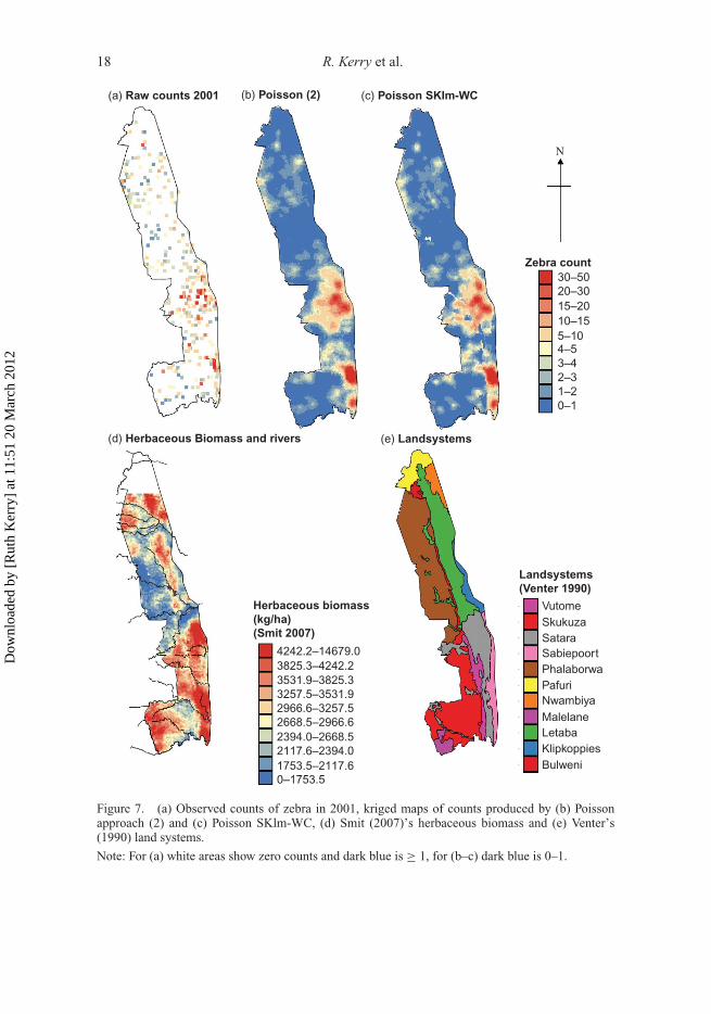
This preliminary analysis was conducted for the 2001 data to illustrate the benefit of incor-porating environmental variables into estimation. The types of environmental data usedare listed in Section 2.2 and two examples, one continuous, variable (herbaceous biomass(B) (Smit 2007), and one categorical variable (LS) (Venter 1990, a classification of thepark into areas of broadly similar geomorphology and vegetation) are shown in Figure 7dand e, respectively. The biomass data could not be incorporated into the SKlm-within-class (WC) approach detailed in Section 2.4.3, but the value of these and other continuousenvironmental data was briefly investigated through Poisson regression. Table 1 shows foreach species the environmental data with significant contributions and regression MAEssmaller than those of Poisson approach (2). Clearly, several of the environmental data setscould be useful in a Poisson kriging approach similar to that of Bellier et al. (2010) whereenvironmental variables are used to determine the trend or local drift in the animal counts.However, for warthog and kudu, none of the available environmental data are useful. Giventhat herbaceous biomass is the continuous variable most frequently identified as significantin Poisson regression (Table 1) and that the LS classification of Venter (1990) includes con-sideration of broad vegetation type, we employed a simple WC approach to SKlm whereonly the categorical data (LS) are used. The approach proceeds in two steps: (1) the aver-age proportion of a species (i.e. local mean) is derived from the secondary information(LS classification) and (2) residuals are interpolated using Poisson kriging and added tothe local mean.

Table 2 lists the St. MAEs achieved for each species using the SKlm-WC approach. Forelephant bulls, the variogram of the class residuals showed no structure and the St. MAEsfor warthog and kudu for SKlm-WC exceed those for Poisson approach (2). This latterresult is probably caused by the lack of significant contribution of these environmentaldata in Poisson regression (Table 1). Until appropriate environmental covariates are foundfor predicting these species, the univariate Poisson approach (2) appears to be one of themost accurate options for mapping species abundance.

The St. MAEs in Table 2 show that SKlm-WC using the LS classification outperformsPoisson approach (2) for giraffe, impala, waterbuck, wildebeest and zebra. For waterbuckand wildebeest, the order of magnitude drop in St. MAEs (Table 2) for SKlm-WC com-pared with Poisson approach (2) clearly shows the benefit of the simple LS classificationfor predicting the location of these species. For some species (giraffe, impala and zebra),there is little difference in St. MAEs for Poisson approach (2) and SKlm-WC. In particu-lar, the maps for zebra display only minor differences which occur mainly in some isolatedareas of the Letaba landsystem (Figure 7e), where medium counts of zebra are predicteddespite predominantly low counts of zebra being observed (Figure 7c). The analysis heresuggests that the straightforward SKlm-WC approach to incorporating environmental datainto Poisson kriging is useful and, as it only uses one categorical data set, it avoids potentialmulti-colinearity problems.

Dow

nloa

ded

by [

Rut

h K

erry

] at

11:

51 2

0 M

arch

201

2

18 R. Kerry et al.

Zebra count30–50

20–30

15–20

10–15

5–104–5

3–4

2–3

1–2

0–1

Landsystems(Venter 1990)

Vutome

Skukuza

Satara

Sabiepoort

Phalaborwa

Pafuri

Nwambiya

Malelane

Letaba

Klipkoppies

Bulweni

Herbaceous biomass(kg/ha)(Smit 2007)

4242.2–14679.0

3825.3–4242.2

3531.9–3825.3

3257.5–3531.9

2966.6–3257.5

2668.5–2966.6

2394.0–2668.5

2117.6–2394.0

1753.5–2117.60–1753.5

(d) Herbaceous Biomass and rivers (e) Landsystems

(c) Poisson SKIm-WC(b) Poisson (2)(a) Raw counts 2001

N

Figure 7. (a) Observed counts of zebra in 2001, kriged maps of counts produced by (b) Poissonapproach (2) and (c) Poisson SKlm-WC, (d) Smit (2007)’s herbaceous biomass and (e) Venter’s(1990) land systems.

Note: For (a) white areas show zero counts and dark blue is ≥ 1, for (b–c) dark blue is 0–1.

Dow

nloa

ded

by [

Rut

h K

erry

] at

11:

51 2

0 M

arch

201

2


4. Conclusions

This study indicated that multiple indicator kriging is less accurate than Poisson kriging formapping animal abundance. Regardless of whether raw count or migrated data are used, therare occurrences of large counts cause only a few indicator variograms to show any struc-ture and the number of thresholds had to be reduced. The total population estimates derivedfrom this method were more than an order of magnitude too low, and the pure nuggetindicator variograms for all thresholds make this method of no use at all for mapping thelower density species.

Based on St. MAEs, Poisson approach (1) is more suitable for mapping the more abun-dant species and Poisson approach (2) for less abundant species. Total population estimatesfor all species derived from area-to-point Poisson kriging approach (2) are similar to thoseproduced by the distance method (results for impala only are shown in Figure 1b), the cur-rent method used by KNP to estimate total species populations in the park. The benefit ofarea-to-point Poisson kriging is its ability to produce accurate maps of species distributionsin addition to sensible total population totals. The uncertainty attached to the total popu-lation estimates produced by area-to-point Poisson kriging methods needs to be modelledusing stochastic simulation for a proper comparison with the distance method in this aspect.

Incorporating environmental data in Poisson approach (2) reduced St. MAEs for mostspecies, particularly for waterbuck and wildebeest. As warthog and kudu abundance wasnot significantly related to any of the available environmental data, suitable environmentalcovariates need to be found for these species. Potential covariates are abundance patternsof these species from previous years when the whole park was surveyed. This prelimi-nary study illustrated the utility of a straightforward SKlm-WC approach, however, giventhe range of variables identified as significant in Poisson regression; more complex meth-ods that incorporate various continuous and categorical environmental data into Poissonkriging are worth investigating.

Poisson approaches that incorporate secondary information are recommended for map-ping species abundance wherever suitable environmental data and sufficient knowledge ofthe environmental factors that are linked to the distribution of a particular species are avail-able. In particular, Bellier et al. (2010) showed that taking account of the heterogeneity ofwildlife population habitats (i.e. non-stationarity in spatial trends) in Poisson kriging leadsto different estimates in sparsely sampled areas (extrapolation situation). If such informa-tion is not available or until more exhaustive research of the best environmental covariatesis done, Poisson approach (1) is recommended for mapping relatively abundant species andPoisson approach (2) for less abundant species. Using such approaches that consider onlyspatial autocorrelation is sensible in such instances because the spatial autocorrelation inanimal counts is likely to reflect indirectly the social behaviour of the species or spatialautocorrelation in the environmental characteristics that influence its distribution.

AcknowledgementsThe research by the second author was funded by grant R44-CA132347-02 from the National CancerInstitute. The views stated in this publication are those of the author and do not necessarily representthe official views of the NCI. The authors thank Judith Botha (SANParks) for supplying the rawaerial survey data and the associated ‘DISTANCE’ estimates.

ReferencesBellier, E., Monestiez, P., and Guinet, C., 2010. Geostatistical modelling of wildlife populations: a

non-stationary hierarchical model for count data. In: P.M. Atkinson and C.D. Lloyd, eds. GeoenvVii – geostatistics for environmental applications. Dordrecht: Springer, 1–12.

Dow

nloa

ded

by [

Rut

h K

erry

] at

11:

51 2

0 M

arch

201

2

20 R. Kerry et al.

BioMedware, Inc., 2011. SpaceStat user manual version 2.2. Ann Arbor, MI: BioMedware.Bucini, G., et al., 2010. Woody fractional cover in Kruger National Park, South Africa: remote-

sensing-based maps and ecological insights. In: M.J. Hill and N.P. Hanan, eds. Ecosystemfunction in savannas: measurement and modeling at landscape to global scales. Boca Raton,FL: CRC/Taylor and Francis, 219–237.

Buckland, S.T., et al., 1993. Introduction to distance sampling: estimating abundance of biologicalpopulations. Oxford: Oxford University Press.

Deutsch, C. V. and Journel, A. G., 1998. GSLIB: Geostatistical Software Library, 2nd ed. New York:Oxford University Press.

Gertenbach, W.P.D., 1983. Landscapes of the Kruger National Park. Koedoe, 26, 9–121.Goovaerts, P., 1994. Comparative performance of indicator algorithms for modeling conditional

probability distribution functions. Mathematical Geology, 26, 389–411.Goovaerts, P., 2005. Geostatistical analysis of disease data: estimation of cancer mortality risk from

empirical frequencies using Poisson kriging. International Journal of Health Geographics, 4, 31.Goovaerts, P., 2008. Kriging and semivariogram deconvolution in the presence of irregular geograph-

ical units. Mathematical Geosciences, 40, 101–128.Goovaerts, P., 2009. AUTO-IK: a 2D indicator kriging program for the automated non-parametric

modeling of local uncertainty in earth sciences. Computers & Geosciences, 35, 1255–1270.Goovaerts, P., Webster, R., and Dubois, J.P., 1997. Assessing the risk of soil contamination in the

Swiss Jura using indicator geostatistics. Environmental and Ecological Statistics, 4, 31–48.Gotway, C.A., et al., 1996. Comparison of kriging and inverse-distance methods for mapping soil

parameters. Soil Science Society of America Journal, 60, 1237–1247.Harrington, R., et al., 1999. Establishing the causes of the roan antelope decline in the Kruger

National Park, South Africa. Biological Conservation, 90, 69–78.Hendry, O., 2004. Kruger Park ecozone map. Johannesburg: Jacana Media.Kerry, R., et al., 2010. Geostatistical analysis of car theft and robbery in the Baltic states.

Geographical Analysis, 42, 53–77.Kerry, R. and Oliver, M.A., 2003. Variograms of ancillary data to aid sampling for soil surveys.

Precision Agriculture, 4, 261–278.Kerry, R. and Oliver, M.A., 2007a. Determining the effect of asymmetric data on the variogram.

I. Underlying asymmetry. Computers & Geosciences, 33, 1212–1232.Kerry, R. and Oliver, M.A., 2007b. Determining the effect of asymmetric data on the variogram.

II. outliers. Computers & Geosciences, 33, 1233–1260.Kravchenko, A. and Bullock, D.G., 1999. A comparative study of interpolation methods for mapping

soil properties. Agronomy Journal, 91, 393–400.Kruger, J.M., Reilly, B.K., and Whyte, I.J., 2008. Application of distance sampling to estimate

population densities of large herbivores in Kruger National Park. Wildlife Research, 35, 371–376.Kshatriya, M., Cosner, C., and van Jaarsveld, A.S., 2001. Early detection of declining populations

using floor and ceiling models. Journal of Animal Ecology, 70, 906–914.Kyriakidis, P., 2004. A geostatistical framework for area-to-point spatial interpolation. Geographical

Analysis, 36, 259–289.Lark, R.M., 2000. A comparison of some robust estimators of the variogram for use in soil survey.

European Journal of Soil Science, 51, 137–157.Lark, R.M., 2002. Robust estimation of the pseudo cross-variogram for cokriging soil properties.

European Journal of Soil Science, 53, 253–270.Lark, R.M., 2003. Two robust estimators of the cross-variogram for multivariate geostatistical

analysis of soil properties. European Journal of Soil Science, 54, 187–201.Lee, J.J., et al., 2007. Evaluation of potential health risk of arsenic-affected groundwater using

indicator kriging and dose response model. Science of the Total Environment, 384, 151–162.Lin, Y.P., et al., 2002. Factorial and indicator kriging methods using a geographic information system

to delineate spatial variation and pollution sources of soil heavy metals. Environmental Geology,42, 900–909.

Liu, C.W., Jang, C.S., and Liao, C.M., 2004. Evaluation of arsenic contamination potential usingindicator kriging in the Yun-Lin aquifer (Taiwan). Science of the Total Environment, 321,173–188.

Monestiez, P., et al., 2006. Geostatistical modelling of spatial distribution of Balaenoptera physalusin the Northwestern Mediterranean Sea from sparse count data and heterogeneous observationefforts. Ecological Modelling, 193, 615–628.

Dow

nloa

ded

by [

Rut

h K

erry

] at

11:

51 2

0 M

arch

201

2


Ogutu, J.O., et al., 2006. Efficiency of strip- and line-transect surveys of African savanna mammals.Journal of Zoology, 269, 149–160.

Ogutu, J.O. and Owen-Smith, N., 2003. ENSO, rainfall and temperature influences on extremepopulation declines among African savanna ungulates. Ecology Letters, 6, 412–419.

Owen-Smith, N. and Mills, M.G.L., 2006. Manifold interactive influences on the populationdynamics of a multispecies ungulate assemblage. Ecological Monographs, 76, 73–92.

Palma, L., Beja, P., and Rodrigues, M., 1999. The use of sighting data to analyse Iberian lynx habitatand distribution. Journal of Applied Ecology, 36, 812–824.

Redfern, J.V., et al., 2002. Biases in estimating population size from an aerial census: a case study inthe Kruger National Park, South Africa. South African Journal of Science, 98, 455–461.

Rossi, R.E., et al., 1992. Geostatistical tools for modeling and interpreting ecological spatialdependence. Ecological Monographs, 62, 277–314.

Saito, H. and Goovaerts, P., 2002. Accounting for measurement error in uncertainty modelingand decision-making using indicator kriging and p-field simulation: application to a dioxincontaminated site. Environmetrics, 13, 555–567.

Saito, H. and McKenna, S.A., 2007. Delineating high-density areas in spatial Poisson fieldsfrom strip-transect sampling using indicator geostatistics: application to unexploded ordnanceremoval. Journal of Environmental Management, 84, 71–82.

Smit, I.P.J., 2007. Artificial surface-water provision in a semi-arid savanna: a spatio-temporal anal-ysis of herbivore distribution patterns in relation to artificial waterholes under different habitat,rainfall and management scenarios in the Kruger National Park, South Africa. Unpublished PhDthesis. University of Cambridge.

Smit, I.P.J., 2011. Resources driving landscape-scale distribution patterns of grazers in an Africansavanna. Ecography, 34, 67–74.

Smit, I.P.J. and Ferreira, S.M., 2010. Management intervention affects river-bound spatial dynamicsof elephants. Biological Conservation, 143, 2172–2181.

Smit, I.P.J. and Grant, C.C., 2009. Managing surface-water in a large semi-arid savanna park: effectson grazer distribution patterns. Journal for Nature Conservation, 17, 61–71.

Steffens, F.E., 1992. Geostatistical estimation of animal abundance in the Kruger National Park,South Africa. In: A. Soares, ed. Geostatistics Troia ’92. Kluwer: Dordrecht, 887–897.

Thomas, L., et al., 2004. Distance 4.1. Release 2. (Research unit for wildlife population assessment).St Andrews: University of St Andrews.

Vandermeer, J. and Leopold, M.F., 1995. Assessing the population-size of the European storm-petrel(Hydrobates pelagicus) using spatial autocorrelation between counts from segments of crisscrossship transects. ICES Journal of Marine Science, 52, 809–818.

Van Meirvenne, M. and Goovaerts, P., 2001. Evaluating the probability of exceeding a site-specificsoil cadmium contamination threshold. Geoderma, 102, 75–100.

Venter, F.J., 1990. A classification of land for management planning in the Kruger National Park.Unpublished PhD thesis. University of South Africa, Pretoria.

Voltz, M. and Webster, R., 1990. A comparison of kriging, cubic splines and classification forpredicting soil properties from sample information. The Journal of Soil Science, 41, 473–490.

Dow

nloa

ded

by [

Rut

h K

erry

] at

11:

51 2

0 M

arch

201

2

A comparison of multiple indicator kriging and area-to-point Poisson kriging for mapping patterns of...

Documents

Transcript of A comparison of multiple indicator kriging and area-to-point Poisson kriging for mapping patterns of...