Universiteit Leiden

Opleiding Informatica

A Comparison of Methods for Predicting Football Matches

Name: David B. EkefreStudentnr: s1470655

Date: 14/02/2016

1st supervisor: Jan N. van Rijn2nd supervisor: Dr. A.J. (Arno) Knobbe

MASTER’S THESIS

Leiden Institute of Advanced Computer Science (LIACS)Leiden UniversityNiels Bohrweg 12333 CA LeidenThe Netherlands

Abstract

Data analysis (or Data mining) has become a major part of ourbusinesses, governments and lives. The concept of analyzing the thingsthat happen around us in our everyday life could be said to be humannature — making sense of our environment, the people around us, howwe and/or the people around us live their lives and drawing conclusionsfrom these observations. Data mining, in this sense, is observing astream of data or a static dataset, using algorithms to make sense ofthe data or find patterns, have a target or conclusion in mind youwant the algorithm to draw from the data (inductive) or you allowthe algorithm to draw its own conclusions from the data (deductive);whichever way, new insights and conclusions are drawn.

Data mining is now being used in sports. In Association Football(football), the sports seen as the most popular sports in the world,data mining has been a big part of the sport as a cooperate business,a betting business, gaming industry business.

There are different methods that have been proposed for predict-ing a football match but in this thesis paper, we do not propose onemethod or any method for predicting a football match. We show acomparison of different methods using feature selection from mainlyhistorical data; and show if using football team formations (or tac-tics) as dependent features add any significant value to the predictinga football match. However, the team formation data used in this the-sis has limited information due to the difficulty in acquiring footballdata in the world today.

1

Contents

1 INTRODUCTION 41.1 Problem Statement . . . . . . . . . . . . . . . . . . . . . . . . 51.2 Comparison of Methods & Feature Selection . . . . . . . . . . 5

2 LITERATURE 6

3 EXPERIMENTS 123.1 Dataset . . . . . . . . . . . . . . . . . . . . . . . . . . . . . . 123.2 Team Form . . . . . . . . . . . . . . . . . . . . . . . . . . . . 133.3 Team Home & Away Form . . . . . . . . . . . . . . . . . . . . 173.4 Match Statistics . . . . . . . . . . . . . . . . . . . . . . . . . . 213.5 Team Formation . . . . . . . . . . . . . . . . . . . . . . . . . 24

3.5.1 Binning by equal width . . . . . . . . . . . . . . . . . . 243.5.2 Binning by equal frequency . . . . . . . . . . . . . . . 25

3.6 Formation Clustering . . . . . . . . . . . . . . . . . . . . . . . 263.6.1 Formation Clustering . . . . . . . . . . . . . . . . . . . 263.6.2 Comparison of Accuracy . . . . . . . . . . . . . . . . . 33

3.7 Shot-Driven Results . . . . . . . . . . . . . . . . . . . . . . . . 343.8 Learning Curve . . . . . . . . . . . . . . . . . . . . . . . . . . 35

4 DISCUSSION 364.1 Team Form . . . . . . . . . . . . . . . . . . . . . . . . . . . . 364.2 Team Home & Away Form . . . . . . . . . . . . . . . . . . . . 374.3 Match Statistics . . . . . . . . . . . . . . . . . . . . . . . . . . 384.4 Team Formation . . . . . . . . . . . . . . . . . . . . . . . . . 38

4.4.1 Binning by equal width . . . . . . . . . . . . . . . . . . 394.4.2 Binning by equal frequency . . . . . . . . . . . . . . . 43

4.5 Formation Clustering . . . . . . . . . . . . . . . . . . . . . . . 444.6 Shot-Driven Results . . . . . . . . . . . . . . . . . . . . . . . . 45

5 CONCLUSION & FUTURE WORK 475.1 Conclusion . . . . . . . . . . . . . . . . . . . . . . . . . . . . . 475.2 Future Work . . . . . . . . . . . . . . . . . . . . . . . . . . . . 48

AA description of Dataset 49

2

BTeam Formation Partitions 49

CA description of Attributes 50

DPaired T-test Results 51

EExpert constructed Bayesian Network 51

FA more detailed explanation on pi-football Components 52

References 55

3

1 INTRODUCTION

Data analysis (or Data mining) has become a major part of our businesses,governments and lives. The concept of analyzing the things that happenaround us in our everyday life could be said to be human nature — makingsense of our environment, the people around us, how we and/or the peoplearound us live their lives and drawing conclusions from these observations.Data mining, in this sense, is observing a stream of data or a static dataset,using algorithms to make sense of the data or find patterns, have a targetor conclusion in mind you want the algorithm to draw from the data (induc-tive) or you allow the algorithm to draw its own conclusions from the data(deductive); whichever way, new insights and conclusions are drawn. Datamining is said to give answers to questions you never thought were there.

Data mining is now being used in sports. In Association Football (foot-ball1), the sports seen as the most popular sports in the world, data mininghas been a big part of the sport as a cooperate business, a betting business,gaming industry business. Data mining is a big part of the football cooperatebusiness by determining the worth of players bought into a club and sold outof a club, by determining how players’ health are managed individually aswell as collectively, how players are told to play and many more. The footballbetting industry business, however, has been an active business long beforedata mining was introduced to it but as every other industry, with the intro-duction of technology and more specifically, data mining, there becomes anexponential growth in the amount of business that can be done in a quickerbut more efficient way. Having said this, data mining in the football bettingindustry has brought about more efficient ways of predicting the outcome ofa single football game, to the extent that even the minor details that go onin a football game like the amount of corners, who gets the first goal kickor which player gets the first booking of the game is being predicted on adaily basis; league positions are also being predicted and bookmaker oddshave become more profitable with the use of data mining techniques amongstmany advantages data mining has brought to the football betting industrybusiness. In the football gaming industry, data mining has been instrumen-tal in determining the realism of in-game tactics — how tactics are executedin-game by video game teams are becoming more and more like how tacticsare being executed in-game in real life.

1From henceforth in this paper it will be called football

4

1.1 Problem Statement

Companies and organizations like OPTA, STATS and ProZone [3, 27]gather and analyze sports data in high volumes, velocities and varieties.These companies gather football data such as players’ performances, heatmap activities, historical data amongst many other football data they gather.They gather these data to create new insight into player and team perfor-mances, tactical insights, team strengths and match predictions. Data min-ing techniques like classification and regression models have been used tomake match predictions. Predicting the outcome of a football match prior towhen that football match is played can be said to be a million dollar industry,hence, football match predictions is a very interesting subject in the area ofsports data analysis.

Papers like have researched on the efficiency of football match predic-tions, more specifically by bookmakers of the betting industry. Differentmethods have been proposed over the years on how to predict a footballmatch. Some methods are derived using just quantitative data and someusing just qualitative data while others use a mixture of both quantitativeand qualitative data in predicting football matches. A quantitative datasetwould be a dataset that consists of historical data like head-to-head results,recent performances or shots on target while a qualitative dataset would con-sist of expert knowledge on team and player performance, player availabilityor media pressure. Although, these methods propose one way, respective totheir various methods, making a comparison of various methods that can beused to predict the outcome of a football match is a not so common approachto football match prediction research papers.

1.2 Comparison of Methods & Feature Selection

In this paper, we do not propose any specific methods for predicting foot-ball matches but rather explore various methods using data mining tech-niques. We compare these various methods using different data mining clas-sifiers (algorithms) and present the results in a chart. The methods weexplore are a product of feature selection. We select a number of features,features that we presume could affect the outcome of a football match, useeither any or a combination of these features for predictions.

The team formations or tactic, however, is slightly different in the sensethat it is used contingent upon other features. This is due to the limitation of

5

the team formation data we had obtained for this thesis. Gathering footballdata is a million dollar business, and for the fact that this is a master’s studythesis, there was only so much that could be spent on gathering the dataneeded and used for this thesis. The team formation data used in this thesiscan be said to be just a string of numbers, for example, (4-4-2), and is usedcontingent on any or a combination of other features. Features like recentperformance (form) or shots. We were also able to determine, to some extent,in which match scenarios the team formations data would have more value.Match scenarios like when a top league team plays a bottom league teamor a middle league team plays a bottom or top league team — these matchscenarios are determined by the teams’ total form values.

Despite the limited data we were able to gather for this thesis, we posetwo research questions. These questions are:

1. Which features or combination of features would produce better pre-dictions?

2. Do team formations add significant value to football match predic-tions?

In the next chapter, chapter 2, we will talk about previous literature workdone regarding football match predictions. In chapter 3, we will show ourexperiment results and comparisons using different features and in chapter4, the discussion chapter, we will give insights and pose questions based onthe results shown in the chapter 3. Finally, in chapter 5, we will concludethis thesis paper and suggest future research in the area of comparing variousmethods and the use of team formations in football match predictions.

2 LITERATURE

The outcome of football matches have been predicted for a very long time,mostly by intuition or “gut” feeling. The first “scientific” model and re-search for predicting the results of football matches was the Poisson modelwhich is modelled after the actual Poisson Distribution named after Frenchmathematician Simeon Denis Poisson.

A Poisson Distribution according to Investopidia, is a “statistical distri-bution showing the frequency probability of specific events when the averageprobability of a single occurrence is known” [19]. The Poisson model usedin predicting football match outcomes is mainly based on the how much ballpossession each team has [22, 24, 9], in respect to scoring when with the ball

6

and not conceding when not with the ball; not necessarily about keeping theball for a certain amount of time. In [34], the author introduced the notionof maximum likelihood estimates, using the 1973 National Football League(NFL) outcome as dataset to conclude, among other things, that the presentranking system of the 1973 NFL season was not a fair ranking system, goingahead to show that the Poisson model — maximum likelihood is a betterranking system; whereas [24] calculates, using a bivariate Poisson model [9],the maximum likelihoods on four parameters — home attack (α), away de-fense (β), home defense (γ) and away attack (δ), he came to the conclusionthat the relative strength of a team’s attack is the same whether home oraway, same about teams’ defense.

The author of [25] uses goals as the parameter to predict game resultsby proving goals in football matches are distributed by negative binomialdistribution, although at that time he had not named the distribution butrather called it the “modified poisson distribution”; not until [30] proved thesame conclusion not only in football matches but in other ball games, cameup with the name of the distribution as “negative binomial”.

Unlike the Poisson models that predict the number of goals scored andconceded, which in turn are used indirectly to predict match outcomes, othermodels are restricted to predicting just the match results i.e win, draw or loss;of course these models consists of various explanatory variables (or features)and are typically ordered probit or logit regression models.

The impact of specific variables or factors on match outcomes have beentaken into consideration in a number of studies. Home advantage has been aforefront factor in many of these studies; the authors in [2] found empiricalevidence that the adoption of artificial playing surfaces, adopted by a fewteams during the 1980s and 1990s, led to a sufficient amount of home advan-taged wins. Similarly, home advantage has been linked to the importance ofcrowd size and crowd density by [26, 28].

While investigating the efficiency of bookmakers’ odds, some other studieshave created models for forecasting football match outcomes, using variousfactors in their models. For example, [21] takes into consideration certaindifferences in teams’ performance, for example, the difference in teams’ av-erage point per game and cumulative points over the season; he also tookthe teams’ cumulative and average goal differences, as well as bookmakers’odds as factors in creating an ordered probit regression model. In [13, 17],the authors use a combination of three factors: teams’ quality — depen-dent on how far back and in what division played in prior to the match in

7

question will data be taken into consideration; recent performance — this in-cludes information regarding the home teams’ most recent home results andaway results as independent variables, same for the away teams; the thirdfactor used is a combination of different other factors, factors like matchsignificance, cup competition involvements, geographical distance and crowdattendance relative to league position.

Models that use team quality ratings or team rankings, as it is also called,have also been considered in some studies. Two of the most popular ratingsystems used in predicting match outcomes are: The ELO ratings system,which was initially developed for calculating the strength of chess players[10], which has subsequently been adopted by other sports including foot-ball; and the FIFA/Coca-Cola World rankings. The adopted ELO ratingsystem assigns, and on a continual basis, updates points to a team depen-dent on a win, draw or loss, it also includes an interesting variant that allowsthe rating update coefficient k to depend on the goal difference, thus re-warding a 3-0 win more strongly than a 2-1 win. The authors in [18] usedthe ELO2 ratings to predict the outcome of matches and concluded that theELO ratings appear to be useful in encoding information of past results, buttheir forecasts were still under par compared to bookmakers’ odds. In [33],the authors evaluate the efficacy of the FIFA/Coca-Cola World Ranking forpredicting World Cup results and concluded that the FIFA/Coca-Cola WorldRanking are an effective means of predicting World Cup results. In [23], theauthors have also modeled a forecasting system based on ELO ratings alongwith the FIFA/Coca-Cola World rankings for the EURO 2008 tournamentand concluded that bookmakers’ forecasts outperformed their forecasts.

Most of the variables or factors mentioned so far are quantitative vari-ables; variables derived solely from statistical and historical data, for theuse of football match predictions. We have yet to study papers that offerthe qualitative side of football predictions. According to [6], “a numericalapproach to forecasting offers one perspective on fixed sports betting, qual-itative research and judgment another”, proposes that “the most effectiveapproach to sports prediction is likely to make use of both quantitative andqualitative information”. The subjective or qualitative information men-tioned in this research paper may refer to information derived from expertopinion.

2The ELO mentioned here and hereafter means the adopted ELO rating system forfootball.

8

Machine learning techniques are at the forefront of making use of bothquantitative and/or qualitative information for predicting football match out-comes. In [20], the authors concluded that an expert constructed bayesiannetwork model (see Section E for model) built for predicting football matchoutcomes, compared to other machine learning models built using the samedata, performed generally superior. Their bayesian network model was basedalmost exclusively on subjective judgment. Some of the subjective judgmentor information used by the authors include: the identification of ‘special’players, the inclusion or exclusion of these ‘special’ players on match-dayto measure the quality of both teams and the venue where the game is be-ing played. The authors in [4] carried out a performance prediction experi-ment during the European Football Championships in 1996 by relying on theknowledge of four predictors, using evidence theory, an integrating frameworkfor predictions. These four predictors, as called by the authors, which aremainly subjective (qualitative) information are: missing key players, homeadvantage, pressure by media and public and performance of past matches.Although the authors in [4, 20] ended up with positive findings, we can al-ready see the complexity that is found in deriving qualitative information, ascompared to that of deriving quantitative information; this complexity canbe a limitation to making predictions solely on qualitative information andwhile they mainly used subjective information for their models, some otherstudies have had a more balanced approach in using both the qualitativeand quantitative side of information for predictions. For example, in [35],the authors use machine learning techniques such as fuzzy rules, neural net-works and genetic programming techniques for prediction based on a vectorof features. The features used by the authors are the differences of: playerstatuses — injured players, disqualified players, of both teams; score of bothteams over the last five games; team rankings in the current championship;home factor of both teams — the fraction of team total points over teamhome games; and lastly, goal difference, which is goals scored minus goalsconceded, of both teams within a 10 years period. They concluded that thegenetic programming technique was superior for predicting correct results tothe other two methods. The authors in [31] also concluded by claiming thatacceptable match simulation results can be obtained by tuning fuzzy rulesusing tournament data. The fuzzy rules used were determined by parametersof fuzzy-term membership functions and rules weighted by a combination ofgenetic and neural optimization techniques. More importantly for this re-search, the match outcome influencing factors used by the authors were the

9

results of: five previous matches for each team; and the last two head to headresults of both teams in question.

In [7], the authors compare the model proposed with and without sub-jective information and concluded that the subjective information improvedthe model such that the posterior forecasts were on par with bookmakers’performance.The model, which they call ‘pi-football’ (v1.32), develops predictions basedon four generic factors for both the home and away teams; these four fac-tors are: team strength, form, psychology and fatigue. The first component ismainly derived from objective information while the subsequent components,mainly from subjective information.

The authors, after satisfying all four components (see Section F of theAppendix), attempt to assess the quality of their forecast model with andwithout the subjective information against bookmakers’ accuracy and prof-itability. For the accuracy measurement, they chose to use the Rank Prob-ability Score (RPS), and for the profitability measurement, they perform abetting simulation that satisfies the following standard betting rule: “foreach match instance, place a 1-pound bet on the outcome with the highestdiscrepancy, of which the pi-football model predicts with higher probability, ifand only if the discrepancy is greater or equal to 5%”.

They divide their forecast into two separate forecasts: (1) the objectiveforecast generated at component 1, (2) the rather subjective (revised) fore-cast after including components 2, 3 and 4. They are both tested against anormalized bookmakers’ forecast and they concluded that the accuracy of ob-jective forecast was significantly inferior to the bookmakers’ performance butwith the improvement on the objective forecast (which forms the subjectiveforecast), the accuracy becomes on par with the bookmakers’ performance.Suggesting that the bookmakers also make use of subjective information.This supports the claim of [6], that the most effective approach to sportsbetting is to make use of both qualitative and quantitative information.

Regarding the profitability measurement, the subjective forecast was testedagainst the maximum (best available for the bettor) bookmakers’ odds, themean bookmakers’ odds and the most common3 bookmakers’ odds. Theirconclusion was that pi-football was able to generate profit via longshot bets;longshot bets or longshot bias have been identified in [8, 14, 16] as a biasagainst bettors for bookmakers’ profitability, implying that the pi-football

3The most common as at the time the article was written.

10

would have generated higher profits if there were less biased odds. They alsotested the objective forecast against the three bookmakers’ odds and it wasproven, although not much detail was given in the paper about the experi-ment involving the objective forecast, to result in losses. This again suggeststhat the use of subjective information (qualitative) and objective information(quantitative) together gives better performance in sports prediction, eitherfor measuring the accuracy or the profitability of any forecast model.

11

3 EXPERIMENTS

This chapter shows the various experiments carried out in this research andthe respective results. These experiments are carried out using Weka [37]4

and Python [36]5. The dataset is obtained from [11] and [12].There are different ways in which the quality of a forecast model can

be assessed. In particular, we consider just the accuracy for the purpose ofthis research. The machine learning techniques used for these experimentsare: k-Nearest Neighbor (IBk) [1], Random Forest [5], J48 [29] and Boosting(AdaBoostM1) [15].

The attributes (features) used in these experiments are described underSection C of the Appendix.

3.1 Dataset

Our dataset consists of data derived from the past three football seasons(2012/2013, 2013,2014 and 2014/2015) from the five (5) big leagues in Eu-rope, which are the English Premier League, German Bundesliga, FrenchLigue 1, Italian Serie A and the Spanish La Liga, in no order of relevance.Before going into the main experiments of this research, we would like topoint out the diversity of the different leagues in our dataset based on oneattribute, which is the total form. The total form is representative of thecumulative points gathered by each team in the course of a season; thesepoints (cumulative) are then divided by the number of games played (alsocumulative).

The figure below shows two column bars for each of the five leagues; thefirst bar represents the default accuracy value of that league while the secondbar shows the accuracy value based on team league positions of the leaguein question.

4Version 3.7.135Version 2.7.10

12

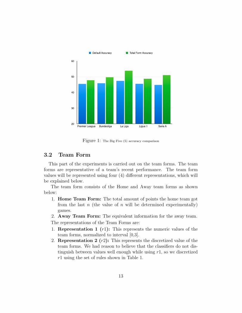
Figure 1: The Big Five (5) accuracy comparison

3.2 Team Form

This part of the experiments is carried out on the team forms. The teamforms are representative of a team’s recent performance. The team formvalues will be represented using four (4) different representations, which willbe explained below.

The team form consists of the Home and Away team forms as shownbelow:

1. Home Team Form: The total amount of points the home team gotfrom the last n (the value of n will be determined experimentally)games.

2. Away Team Form: The equivalent information for the away team.

The representations of the Team Forms are:

1. Representation 1 (r1): This represents the numeric values of theteam forms, normalized to interval [0,3].

2. Representation 2 (r2): This represents the discretized value of theteam forms. We had reason to believe that the classifiers do not dis-tinguish between values well enough while using r1, so we discretizedr1 using the set of rules shown in Table 1.

13

Numeric Values Discretized Values[0,1> Bad Form[1,2> Good Form[2,3] Best Form

Table 1: Numeric & Discretized Values

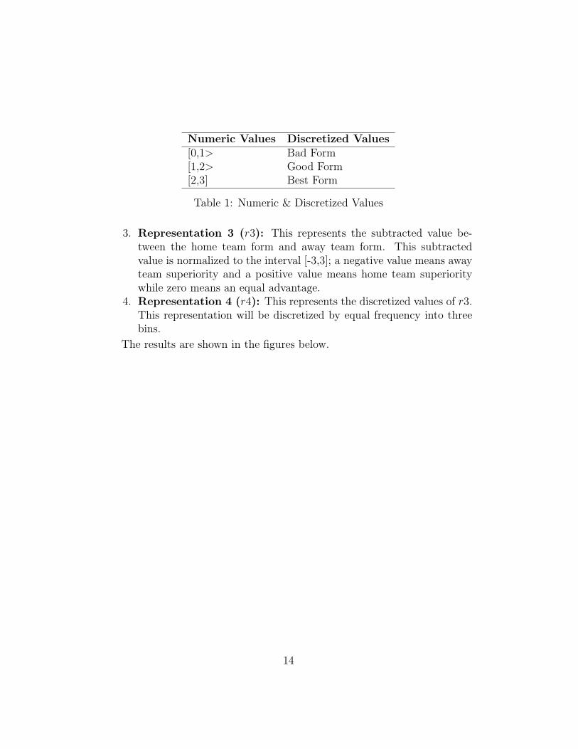
3. Representation 3 (r3): This represents the subtracted value be-tween the home team form and away team form. This subtractedvalue is normalized to the interval [-3,3]; a negative value means awayteam superiority and a positive value means home team superioritywhile zero means an equal advantage.

4. Representation 4 (r4): This represents the discretized values of r3.This representation will be discretized by equal frequency into threebins.

The results are shown in the figures below.

14

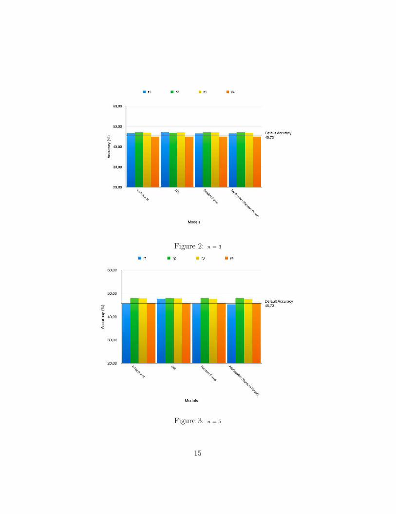
Figure 2: n = 3

Figure 3: n = 5

15

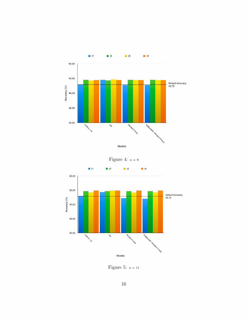
Figure 4: n = 9

Figure 5: n = 11

16

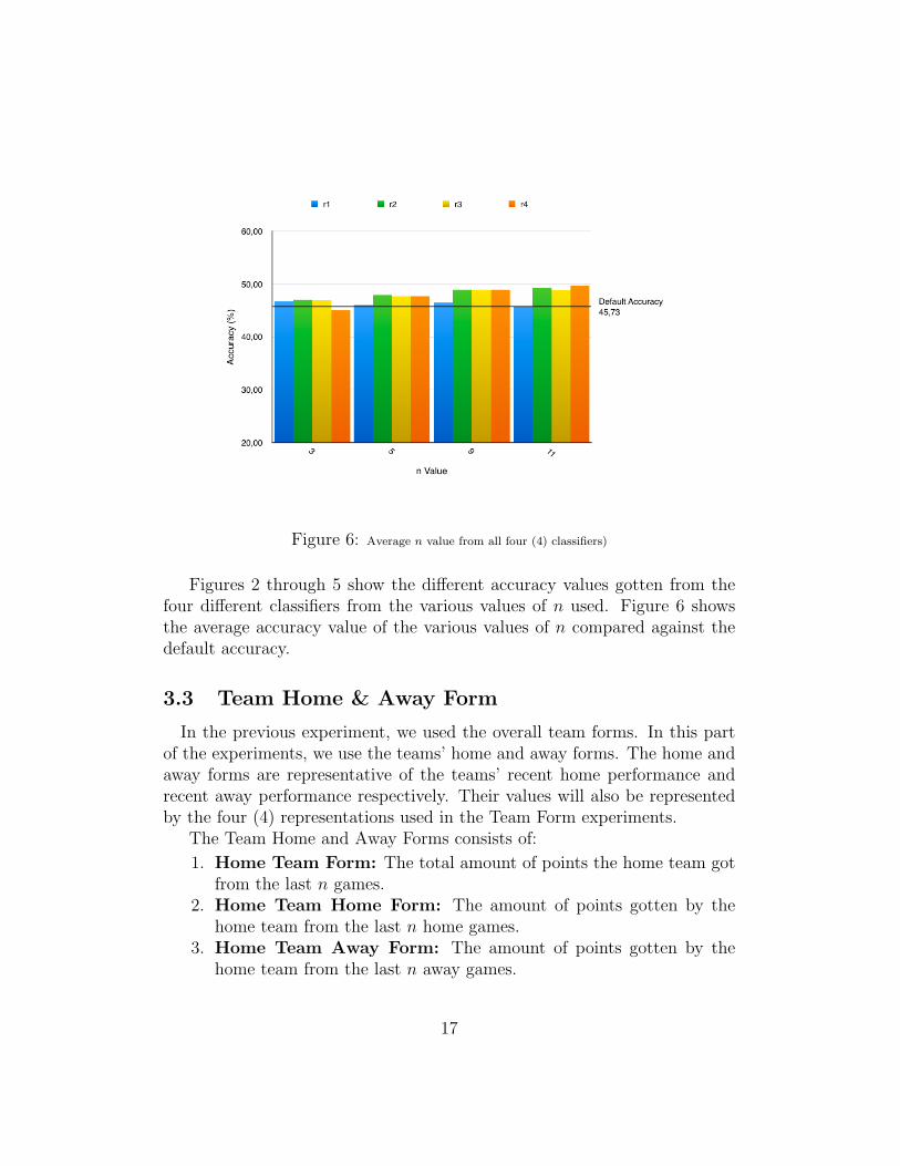
Figure 6: Average n value from all four (4) classifiers)

Figures 2 through 5 show the different accuracy values gotten from thefour different classifiers from the various values of n used. Figure 6 showsthe average accuracy value of the various values of n compared against thedefault accuracy.

3.3 Team Home & Away Form

In the previous experiment, we used the overall team forms. In this partof the experiments, we use the teams’ home and away forms. The home andaway forms are representative of the teams’ recent home performance andrecent away performance respectively. Their values will also be representedby the four (4) representations used in the Team Form experiments.

The Team Home and Away Forms consists of:

1. Home Team Form: The total amount of points the home team gotfrom the last n games.

2. Home Team Home Form: The amount of points gotten by thehome team from the last n home games.

3. Home Team Away Form: The amount of points gotten by thehome team from the last n away games.

17

4. Away Team Form: The equivalent information for the away teamform; Away Team Home Form and Away Team Away Form.

The representations are:

1. Representation 1 (r1): This represents the numeric value of theteam home and away forms, normalized to interval [0,3].

2. Representation 2 (r2): This represents the discretized values, usingthe set of rules shown in Table 1.

3. Representation 3 (r3): This represents the subtracted value be-tween the home team form and away team form; the home team homeform and away team away form; the home team away form and awayteam home form. This subtracted value is normalized to interval [-3,3]. A negative values means away team superiority and a positivevalue means home team superiority.

4. Representation 4 (r4): This represents the discretized values of r3.This representation will be discretized by equal frequency into threebins.

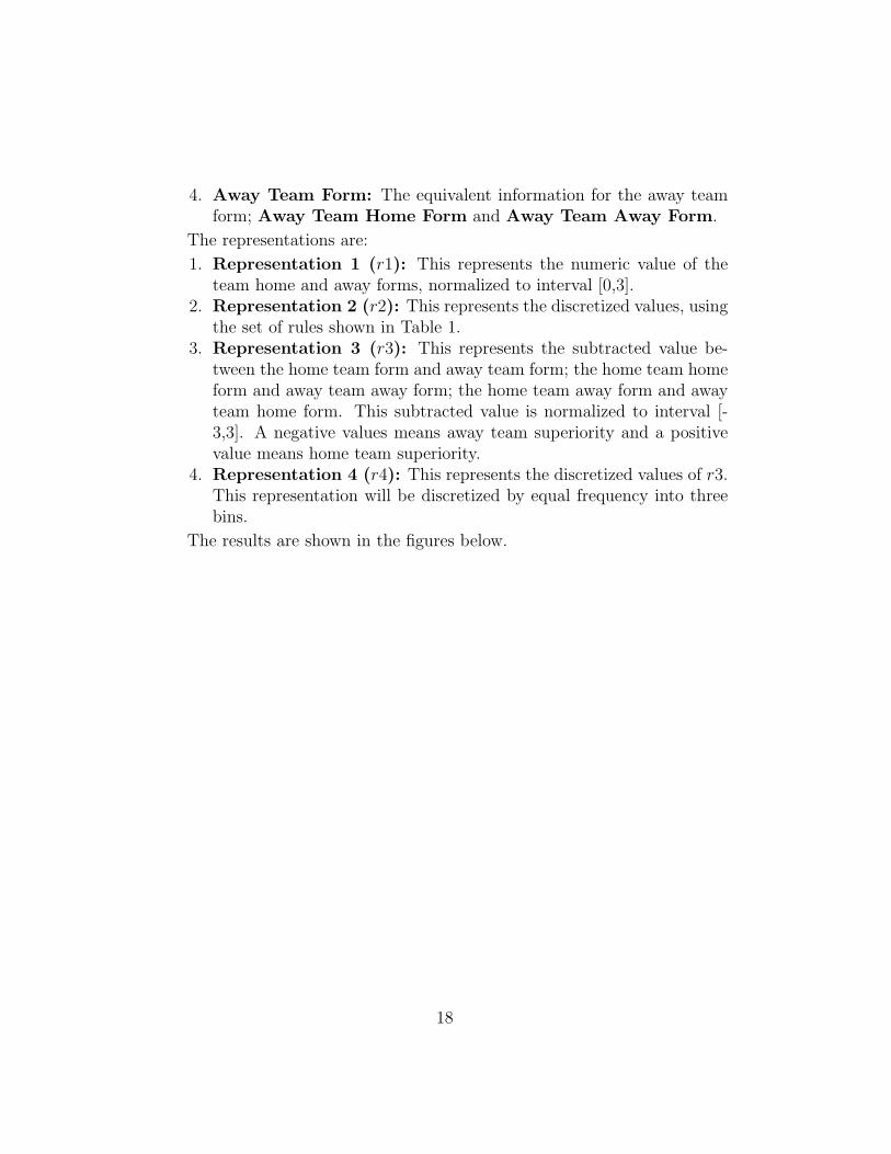
The results are shown in the figures below.

18

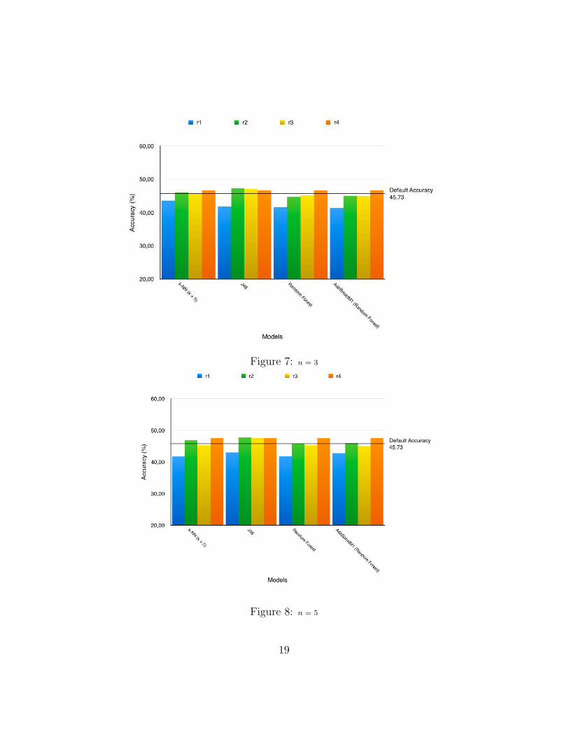
Figure 7: n = 3

Figure 8: n = 5

19

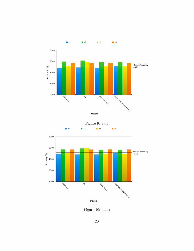
Figure 9: n = 9

Figure 10: n = 11

20

Figure 11: Average n value from all four (4) classifiers

Figures 7 through 10 show the different accuracy values from the fourclassifiers comparing the various values of n used. Figure 11 shows the av-erage accuracy value of the various values of n compared against the defaultaccuracy.

3.4 Match Statistics

In this part of the experiment, we will use a combination of features we callMatch Statistics. Based on the superiority of the discretized values over thenumeric values from the previous experiments, the Match Statistics valueswill be represented using only Representation 4. As mentioned in the earlierexperiments, Representation 4 is discretized by equal frequency into three(3) bins. The value of n used for team forms is set as 9 and 11, also becauseof their superiority over the the two other values of n tested in the previousexperiments.While for the shots and goals attributes only 9 is used as then value.

The Match Statistics features consists of:

1. Goals: The subtracted difference in goals from home and away teamsover 9 games.

21

2. Shots: The subtracted difference in shots from home and away teamsover 9 games.

3. Shots on target: The subtracted difference in shots on target fromhome and away teams over 9 games.

4. Goals Ratio: The subtracted difference in goals ratio from home andaway teams over 9 games.

5. Shots Ratio: The subtracted difference in shots ratio from home andaway teams over 9 games.

6. Form: The subtracted difference in points from home and away teamsover 9 games (represented as Form-9); 11 games (represented asForm-11) and all subsequent games (represented as Total Form).

The attribute selections (or combinations) used are:

1. Attribute Selection 1 (a1): Total Form, Form-9 and Form-11.2. Attribute Selection 2 (a2): Total Form, Shots, Form-9 and Form-

11.3. Attribute Selection 3 (a3): Total Form, Goals, Form-9 and Form-

11.4. Attribute Selection 4 (a4): Total Form, Shots on Target, Form-9

and Form-11.5. Attribute Selection 5 (a5): Total Form, Shots Ratio, Form-9 and

Form-11.6. Attribute Selection 6 (a6):Total Form, Goals Ratio, Form-9 and

Form-11.

The results are shown in the figures below.

22

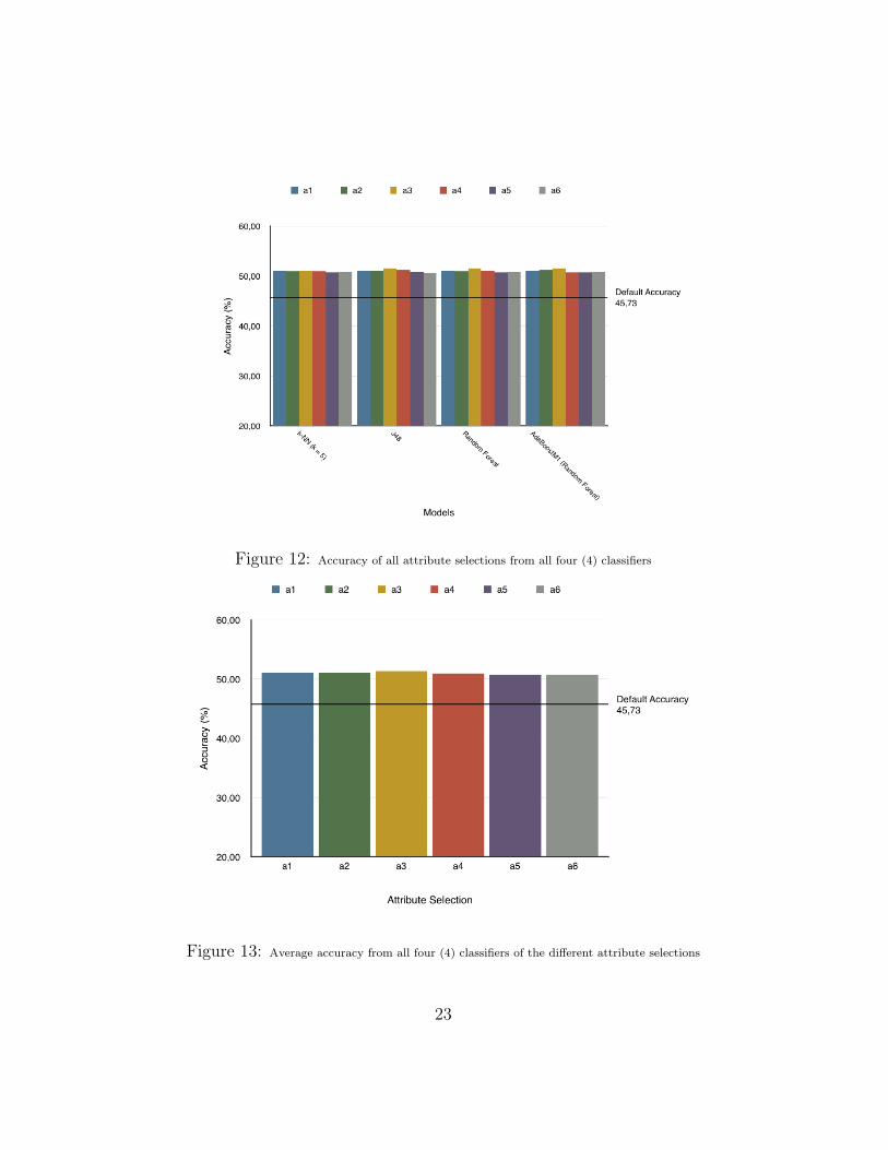
Figure 12: Accuracy of all attribute selections from all four (4) classifiers

Figure 13: Average accuracy from all four (4) classifiers of the different attribute selections

23

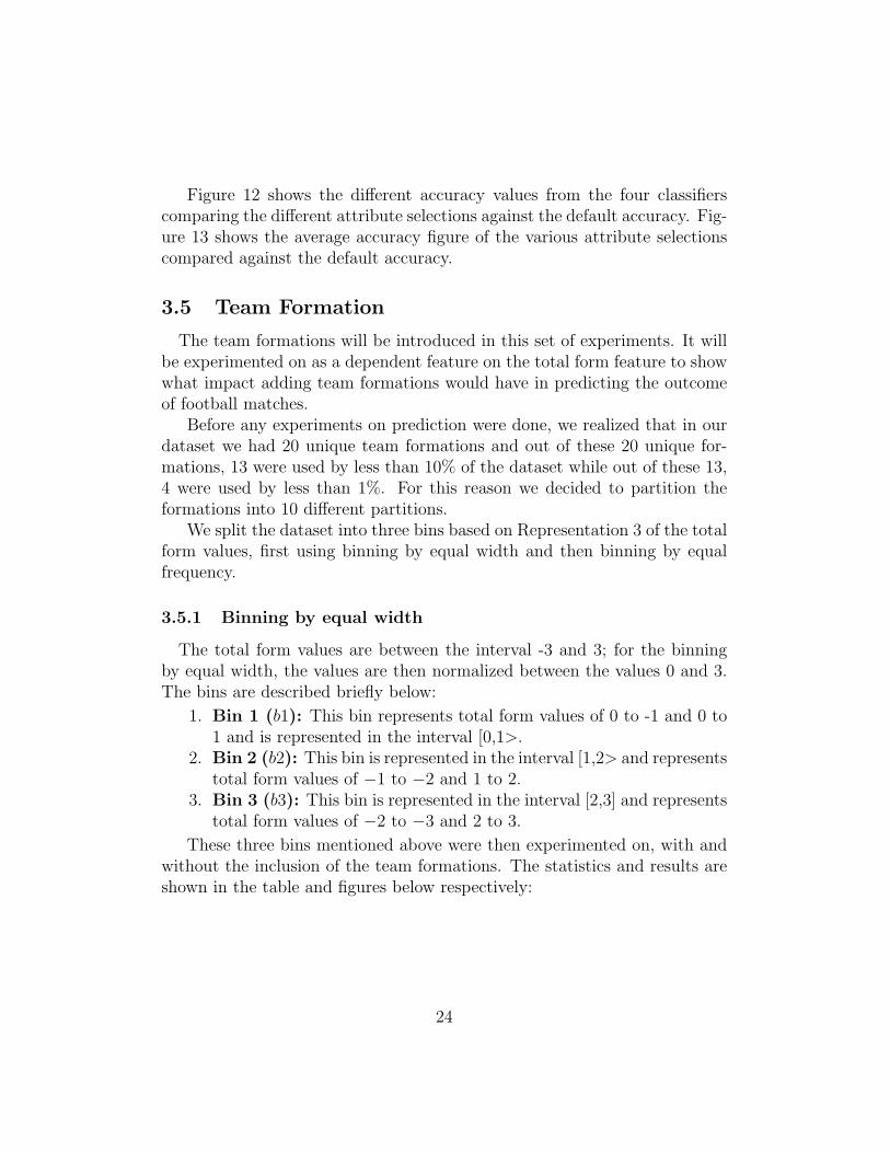
Figure 12 shows the different accuracy values from the four classifierscomparing the different attribute selections against the default accuracy. Fig-ure 13 shows the average accuracy figure of the various attribute selectionscompared against the default accuracy.

3.5 Team Formation

The team formations will be introduced in this set of experiments. It willbe experimented on as a dependent feature on the total form feature to showwhat impact adding team formations would have in predicting the outcomeof football matches.

Before any experiments on prediction were done, we realized that in ourdataset we had 20 unique team formations and out of these 20 unique for-mations, 13 were used by less than 10% of the dataset while out of these 13,4 were used by less than 1%. For this reason we decided to partition theformations into 10 different partitions.

We split the dataset into three bins based on Representation 3 of the totalform values, first using binning by equal width and then binning by equalfrequency.

3.5.1 Binning by equal width

The total form values are between the interval -3 and 3; for the binningby equal width, the values are then normalized between the values 0 and 3.The bins are described briefly below:

1. Bin 1 (b1): This bin represents total form values of 0 to -1 and 0 to1 and is represented in the interval [0,1>.

2. Bin 2 (b2): This bin is represented in the interval [1,2> and representstotal form values of −1 to −2 and 1 to 2.

3. Bin 3 (b3): This bin is represented in the interval [2,3] and representstotal form values of −2 to −3 and 2 to 3.

These three bins mentioned above were then experimented on, with andwithout the inclusion of the team formations. The statistics and results areshown in the table and figures below respectively:

24

Bins Number of Instances[0,1> 4614[1,2> 761[2,3] 30

Table 2: Binning by equal-width Statistics Table

Figure 14: Bins 1 to 3 without formation

Figure 15: Bins 1 to 3 with formation

Figure 14 shows the accuracy of the three (3) bins by equal-width withoutthe inclusion of formations while Figure 15 shows the accuracy with theinclusion of formations. While Figures These results were obtained using theJ48 classifier.

3.5.2 Binning by equal frequency

The original total form values are used. The statistics of the bins are givenin the table below.

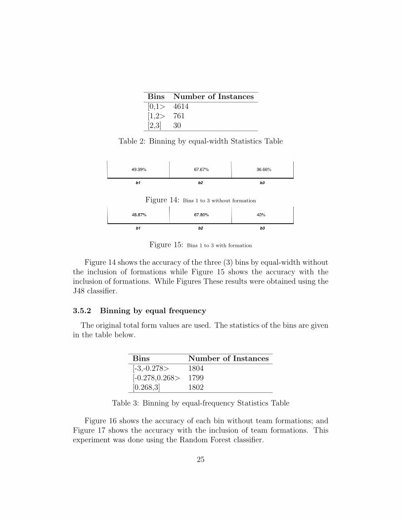
Bins Number of Instances[-3,-0.278> 1804[-0.278,0.268> 1799[0.268,3] 1802

Table 3: Binning by equal-frequency Statistics Table

Figure 16 shows the accuracy of each bin without team formations; andFigure 17 shows the accuracy with the inclusion of team formations. Thisexperiment was done using the Random Forest classifier.

25

Figure 16: Bins 1 to 3 without formation

Figure 17: Bins 1 to 3 with formation

3.6 Formation Clustering

As mentioned in the previous experiment, the team formation experiments,the number of unique team formations found in our dataset is 20. Out ofthese 20 unique formations, 13 of them are used by less than 10% of thedataset while out of these 13, 4 of the team formations are used by less than1%. For this reason, as mentioned earlier, we decided to partition, in thecase of this experiment — cluster the formations.

This experiment will be divided into two parts:

1. The Formation Clustering: this part will show the results derived fromclustering the team formations.

2. Comparison of Accuracy: this part will show the difference in accuracylevels between the clustered formations generated earlier, the parti-tioned formations generated in the ‘Team Formation’ experiments sec-tion and the original dataset team formations.

3.6.1 Formation Clustering

The team formations will be clustered using the hierarchical clusteringmethod. The formation clustering will be based on two sets of attributes:

• shots and;• shots on target.

Both clusters will be made using the average linkage method and the eu-clidean distance function.

The dataset had to be aggregated to the team formations for this ex-periment. For every unique team formation used by the home teams and

26

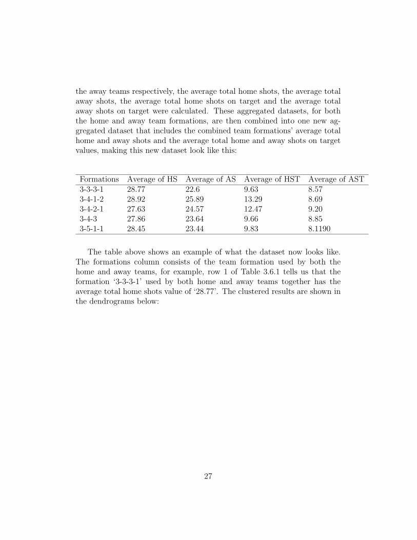
the away teams respectively, the average total home shots, the average totalaway shots, the average total home shots on target and the average totalaway shots on target were calculated. These aggregated datasets, for boththe home and away team formations, are then combined into one new ag-gregated dataset that includes the combined team formations’ average totalhome and away shots and the average total home and away shots on targetvalues, making this new dataset look like this:

Formations Average of HS Average of AS Average of HST Average of AST3-3-3-1 28.77 22.6 9.63 8.573-4-1-2 28.92 25.89 13.29 8.693-4-2-1 27.63 24.57 12.47 9.203-4-3 27.86 23.64 9.66 8.853-5-1-1 28.45 23.44 9.83 8.1190

The table above shows an example of what the dataset now looks like.The formations column consists of the team formation used by both thehome and away teams, for example, row 1 of Table 3.6.1 tells us that theformation ‘3-3-3-1’ used by both home and away teams together has theaverage total home shots value of ‘28.77’. The clustered results are shown inthe dendrograms below:

27

5-3

-2

3-4

-1-2

4-5

-1

4-1

-3-2

4-2

-1-3

3-4

-2-1

5-4

-1

4-4

-2

3-3

-3-1

3-5

-2

3-4

-3

4-2

-3-1

4-3

-3

3-5

-1-1

4-3

-1-2

4-4

-1-1

4-3

-2-1

4-1

-4-1

4-1

-2-3

4-2

-2-2

0.0

0.5

1.0

1.5

2.0

2.5

Hierarchical Clustering Dendrogram

Figure 18: Shots-based Dendrogram

25 26 27 28 29 30 3121

22

23

24

25

26

27

Figure 19: Shots-based 2-d Scatter Plot

28

4-4

-1-1

4-2

-3-1

4-1

-4-1

3-4

-1-2

4-5

-1

3-4

-2-1

4-3

-2-1

5-3

-2

4-1

-2-3

4-4

-2

4-3

-1-2

4-3

-3

3-5

-2

4-2

-2-2

3-4

-3

3-3

-3-1

3-5

-1-1

5-4

-1

4-2

-1-3

4-1

-3-2

0

1

2

3

4

5

Hierarchical Clustering Dendrogram

Figure 20: Shots-on-Target-based Dendrogram

9 10 11 12 13 14 15 16 17 18

6

7

8

9

10

11

12

Figure 21: Shots-on-Target-based 2-d Scatter Plot

29

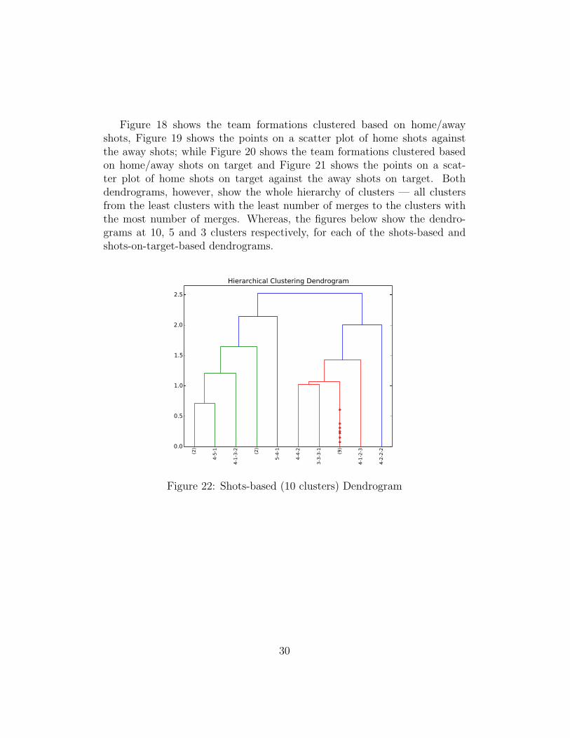
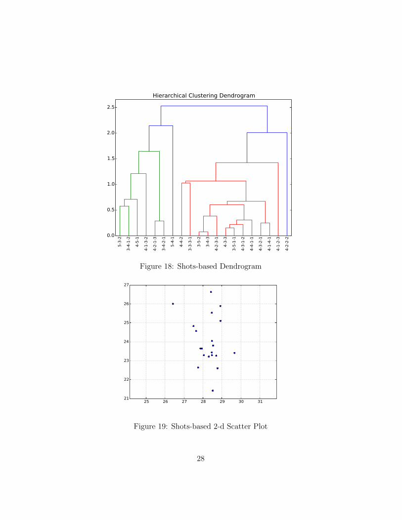
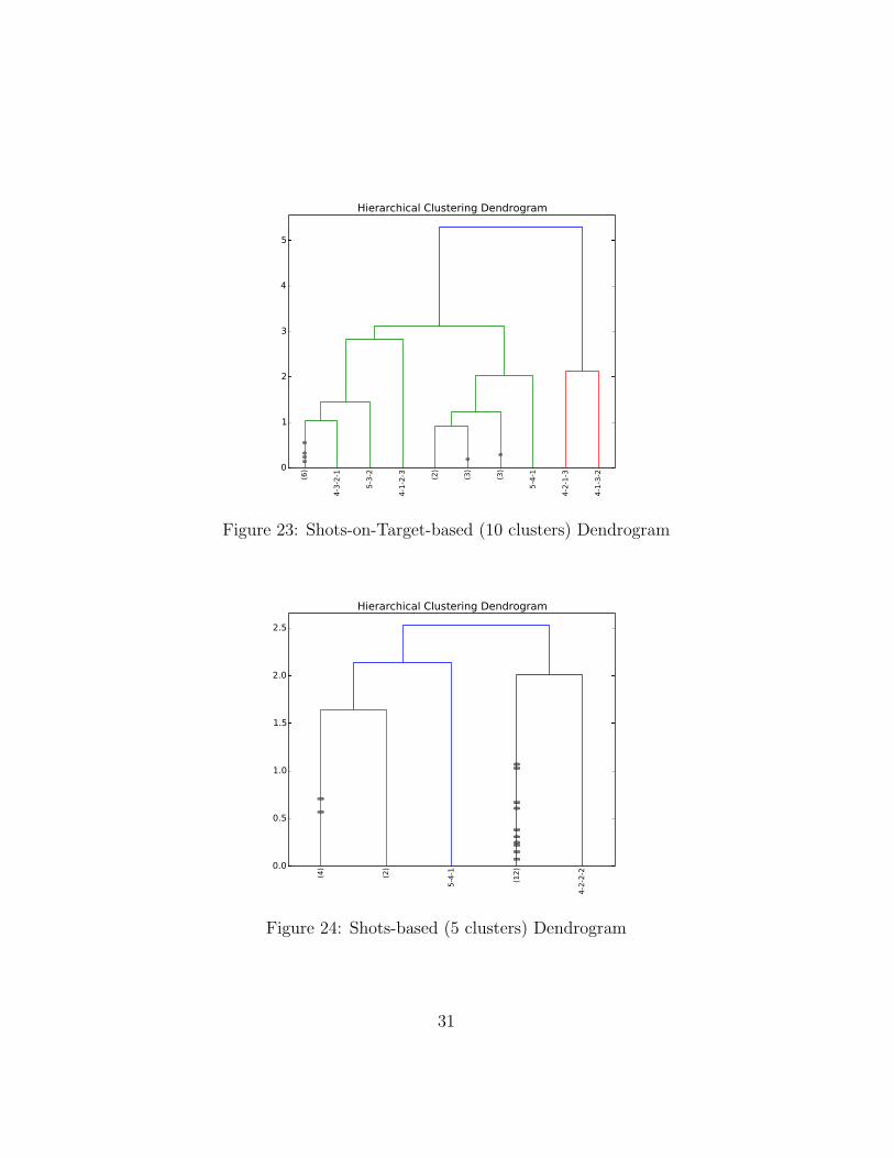
Figure 18 shows the team formations clustered based on home/awayshots, Figure 19 shows the points on a scatter plot of home shots againstthe away shots; while Figure 20 shows the team formations clustered basedon home/away shots on target and Figure 21 shows the points on a scat-ter plot of home shots on target against the away shots on target. Bothdendrograms, however, show the whole hierarchy of clusters — all clustersfrom the least clusters with the least number of merges to the clusters withthe most number of merges. Whereas, the figures below show the dendro-grams at 10, 5 and 3 clusters respectively, for each of the shots-based andshots-on-target-based dendrograms.

(2)

4-5

-1

4-1

-3-2 (2)

5-4

-1

4-4

-2

3-3

-3-1 (9)

4-1

-2-3

4-2

-2-2

0.0

0.5

1.0

1.5

2.0

2.5

Hierarchical Clustering Dendrogram

Figure 22: Shots-based (10 clusters) Dendrogram

30

(6)

4-3

-2-1

5-3

-2

4-1

-2-3 (2

)

(3)

(3)

5-4

-1

4-2

-1-3

4-1

-3-2

0

1

2

3

4

5

Hierarchical Clustering Dendrogram

Figure 23: Shots-on-Target-based (10 clusters) Dendrogram

(4)

(2)

5-4

-1

(12)

4-2

-2-2

0.0

0.5

1.0

1.5

2.0

2.5

Hierarchical Clustering Dendrogram

Figure 24: Shots-based (5 clusters) Dendrogram

31

(8)

4-1

-2-3 (9

)

4-2

-1-3

4-1

-3-2

0

1

2

3

4

5

Hierarchical Clustering Dendrogram

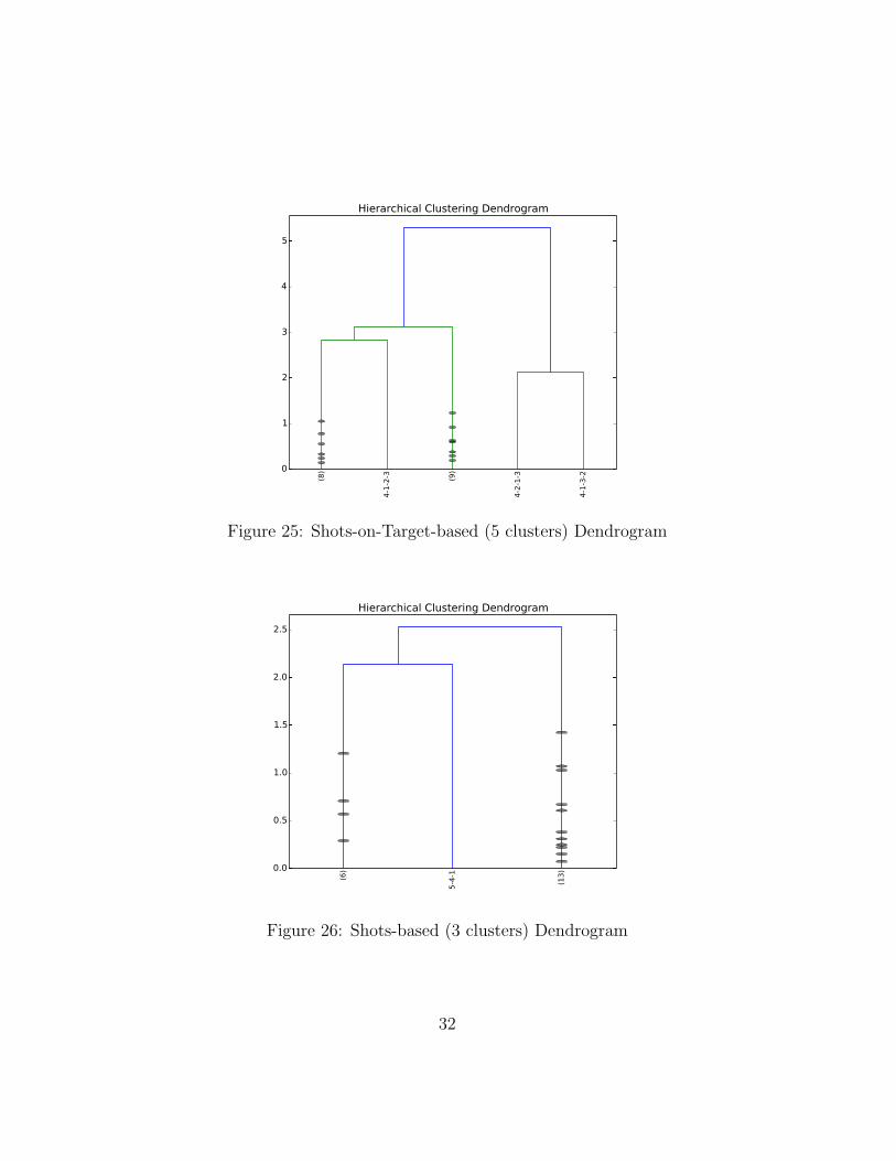
Figure 25: Shots-on-Target-based (5 clusters) Dendrogram

(6)

5-4

-1

(13)0.0

0.5

1.0

1.5

2.0

2.5

Hierarchical Clustering Dendrogram

Figure 26: Shots-based (3 clusters) Dendrogram

32

(9)

(9)

(2)0

1

2

3

4

5

Hierarchical Clustering Dendrogram

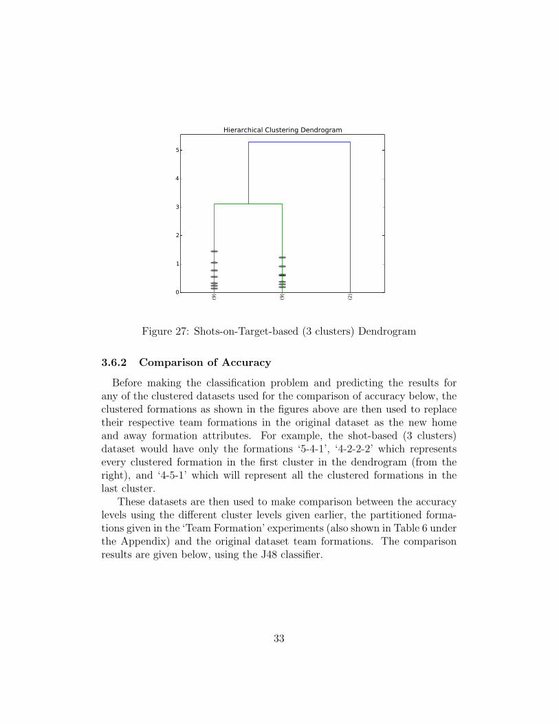
Figure 27: Shots-on-Target-based (3 clusters) Dendrogram

3.6.2 Comparison of Accuracy

Before making the classification problem and predicting the results forany of the clustered datasets used for the comparison of accuracy below, theclustered formations as shown in the figures above are then used to replacetheir respective team formations in the original dataset as the new homeand away formation attributes. For example, the shot-based (3 clusters)dataset would have only the formations ‘5-4-1’, ‘4-2-2-2’ which representsevery clustered formation in the first cluster in the dendrogram (from theright), and ‘4-5-1’ which will represent all the clustered formations in thelast cluster.

These datasets are then used to make comparison between the accuracylevels using the different cluster levels given earlier, the partitioned forma-tions given in the ‘Team Formation’ experiments (also shown in Table 6 underthe Appendix) and the original dataset team formations. The comparisonresults are given below, using the J48 classifier.

33

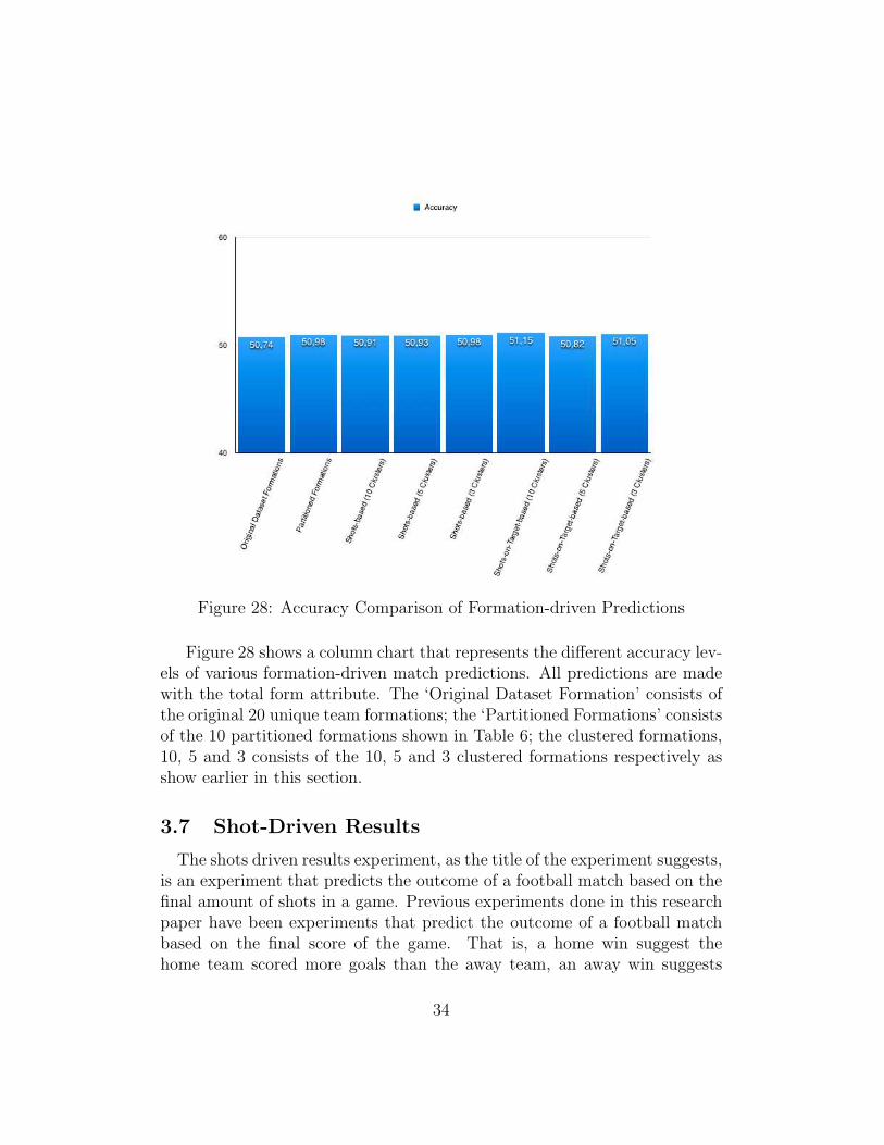
Figure 28: Accuracy Comparison of Formation-driven Predictions

Figure 28 shows a column chart that represents the different accuracy lev-els of various formation-driven match predictions. All predictions are madewith the total form attribute. The ‘Original Dataset Formation’ consists ofthe original 20 unique team formations; the ‘Partitioned Formations’ consistsof the 10 partitioned formations shown in Table 6; the clustered formations,10, 5 and 3 consists of the 10, 5 and 3 clustered formations respectively asshow earlier in this section.

3.7 Shot-Driven Results

The shots driven results experiment, as the title of the experiment suggests,is an experiment that predicts the outcome of a football match based on thefinal amount of shots in a game. Previous experiments done in this researchpaper have been experiments that predict the outcome of a football matchbased on the final score of the game. That is, a home win suggest thehome team scored more goals than the away team, an away win suggests

34

the opposite, while a draw suggests both home and away teams score anequal amount of goals. Whereas, in this experiment, a home win suggeststhe home had more shots in the game, an away win, the opposite, while adraw suggests both teams had an equal amount of shots.

The graph below shows two default accuracy bars and two total formaccuracy bars — the first of either of the default accuracy and total formbars show the accuracy based on the final score of a game while the second ofeach bar shows the accuracy based on the number of shots had by each team.This is to show a comparison of using the shot driven result as opposed tousing the goal driven result.

Figure 29: Comparison of Shot-driven Results and Goal-driven Results

3.8 Learning Curve

The learning curve given below is to experiment on what amount of datais best to use in order to get optimal results. The J48 classifier was used onthe attribute selection a3 from the Match Statistics experiments to createthis learning curve.

The learning curve shows the accuracy at different number of instances.It starts with just ten percent (10%) of the dataset and works its way upthrough ninety percent (90%) of the dataset.

35

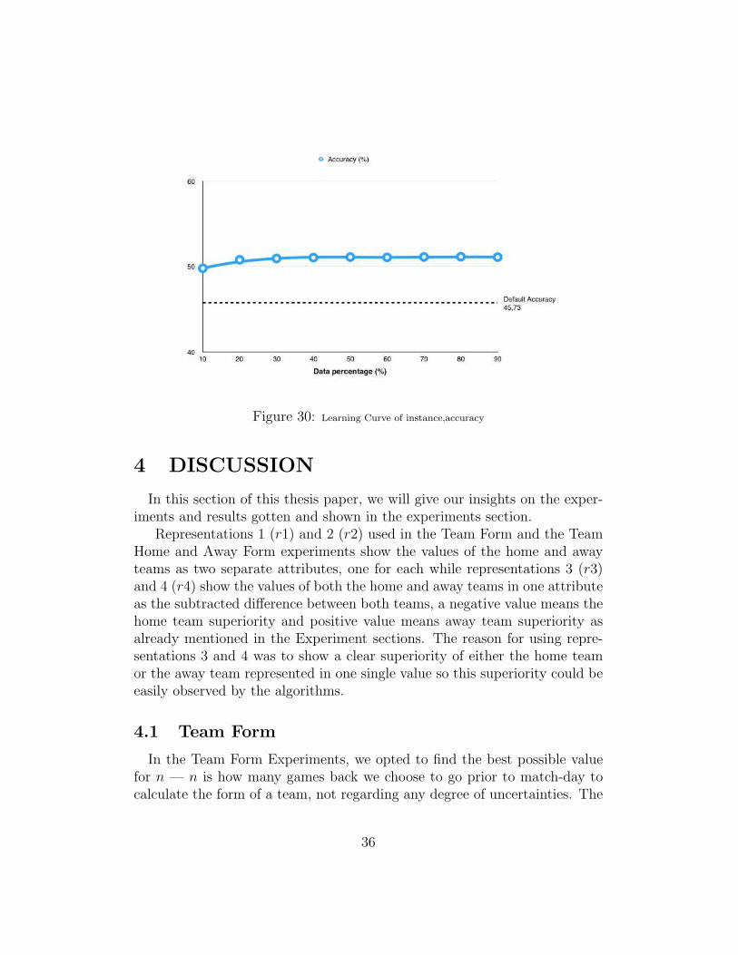
Figure 30: Learning Curve of instance,accuracy

4 DISCUSSION

In this section of this thesis paper, we will give our insights on the exper-iments and results gotten and shown in the experiments section.

Representations 1 (r1) and 2 (r2) used in the Team Form and the TeamHome and Away Form experiments show the values of the home and awayteams as two separate attributes, one for each while representations 3 (r3)and 4 (r4) show the values of both the home and away teams in one attributeas the subtracted difference between both teams, a negative value means thehome team superiority and positive value means away team superiority asalready mentioned in the Experiment sections. The reason for using repre-sentations 3 and 4 was to show a clear superiority of either the home teamor the away team represented in one single value so this superiority could beeasily observed by the algorithms.

4.1 Team Form

In the Team Form Experiments, we opted to find the best possible valuefor n — n is how many games back we choose to go prior to match-day tocalculate the form of a team, not regarding any degree of uncertainties. The

36

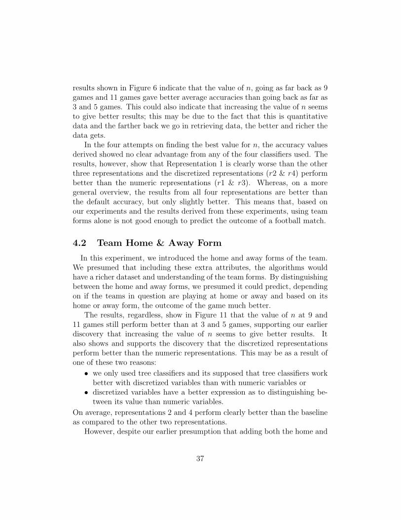
results shown in Figure 6 indicate that the value of n, going as far back as 9games and 11 games gave better average accuracies than going back as far as3 and 5 games. This could also indicate that increasing the value of n seemsto give better results; this may be due to the fact that this is quantitativedata and the farther back we go in retrieving data, the better and richer thedata gets.

In the four attempts on finding the best value for n, the accuracy valuesderived showed no clear advantage from any of the four classifiers used. Theresults, however, show that Representation 1 is clearly worse than the otherthree representations and the discretized representations (r2 & r4) performbetter than the numeric representations (r1 & r3). Whereas, on a moregeneral overview, the results from all four representations are better thanthe default accuracy, but only slightly better. This means that, based onour experiments and the results derived from these experiments, using teamforms alone is not good enough to predict the outcome of a football match.

4.2 Team Home & Away Form

In this experiment, we introduced the home and away forms of the team.We presumed that including these extra attributes, the algorithms wouldhave a richer dataset and understanding of the team forms. By distinguishingbetween the home and away forms, we presumed it could predict, dependingon if the teams in question are playing at home or away and based on itshome or away form, the outcome of the game much better.

The results, regardless, show in Figure 11 that the value of n at 9 and11 games still perform better than at 3 and 5 games, supporting our earlierdiscovery that increasing the value of n seems to give better results. Italso shows and supports the discovery that the discretized representationsperform better than the numeric representations. This may be as a result ofone of these two reasons:

• we only used tree classifiers and its supposed that tree classifiers workbetter with discretized variables than with numeric variables or

• discretized variables have a better expression as to distinguishing be-tween its value than numeric variables.

On average, representations 2 and 4 perform clearly better than the baselineas compared to the other two representations.

However, despite our earlier presumption that adding both the home and

37

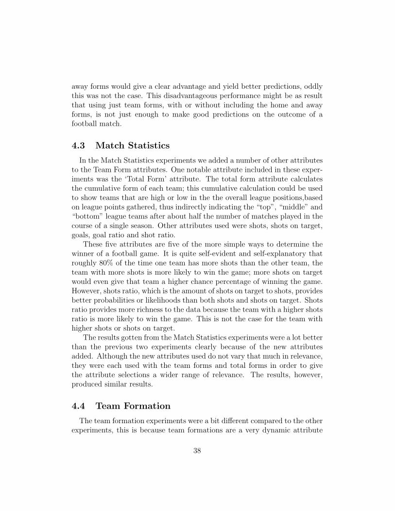
away forms would give a clear advantage and yield better predictions, oddlythis was not the case. This disadvantageous performance might be as resultthat using just team forms, with or without including the home and awayforms, is not just enough to make good predictions on the outcome of afootball match.

4.3 Match Statistics

In the Match Statistics experiments we added a number of other attributesto the Team Form attributes. One notable attribute included in these exper-iments was the ‘Total Form’ attribute. The total form attribute calculatesthe cumulative form of each team; this cumulative calculation could be usedto show teams that are high or low in the the overall league positions,basedon league points gathered, thus indirectly indicating the “top”, “middle” and“bottom” league teams after about half the number of matches played in thecourse of a single season. Other attributes used were shots, shots on target,goals, goal ratio and shot ratio.

These five attributes are five of the more simple ways to determine thewinner of a football game. It is quite self-evident and self-explanatory thatroughly 80% of the time one team has more shots than the other team, theteam with more shots is more likely to win the game; more shots on targetwould even give that team a higher chance percentage of winning the game.However, shots ratio, which is the amount of shots on target to shots, providesbetter probabilities or likelihoods than both shots and shots on target. Shotsratio provides more richness to the data because the team with a higher shotsratio is more likely to win the game. This is not the case for the team withhigher shots or shots on target.

The results gotten from the Match Statistics experiments were a lot betterthan the previous two experiments clearly because of the new attributesadded. Although the new attributes used do not vary that much in relevance,they were each used with the team forms and total forms in order to givethe attribute selections a wider range of relevance. The results, however,produced similar results.

4.4 Team Formation

The team formation experiments were a bit different compared to the otherexperiments, this is because team formations are a very dynamic attribute

38

in a football match. Football is a very dynamic game, dynamic in the sensethat: one minute the odds could be with team a and in the next minuteteam b. Likewise, team formations, in a single game, a team can change itsstarting formation (the formation the team starts the game with) more thanonce. These team formation in-game changes could swing the odds back tothe team’s favor, hence changing the whole dynamic of the game from thatchange of formation. However, the team formation experimented with inthis thesis reflects only the starting team formations, and does not reflectthis dynamic nature of team formations just discussed.

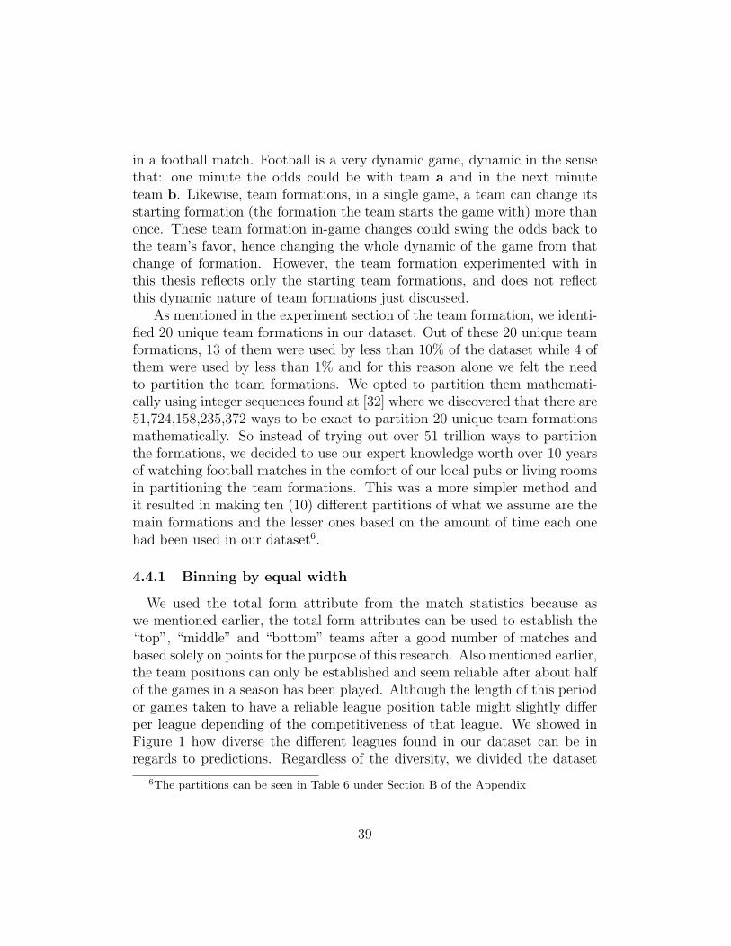
As mentioned in the experiment section of the team formation, we identi-fied 20 unique team formations in our dataset. Out of these 20 unique teamformations, 13 of them were used by less than 10% of the dataset while 4 ofthem were used by less than 1% and for this reason alone we felt the needto partition the team formations. We opted to partition them mathemati-cally using integer sequences found at [32] where we discovered that there are51,724,158,235,372 ways to be exact to partition 20 unique team formationsmathematically. So instead of trying out over 51 trillion ways to partitionthe formations, we decided to use our expert knowledge worth over 10 yearsof watching football matches in the comfort of our local pubs or living roomsin partitioning the team formations. This was a more simpler method andit resulted in making ten (10) different partitions of what we assume are themain formations and the lesser ones based on the amount of time each onehad been used in our dataset6.

4.4.1 Binning by equal width

We used the total form attribute from the match statistics because aswe mentioned earlier, the total form attributes can be used to establish the“top”, “middle” and “bottom” teams after a good number of matches andbased solely on points for the purpose of this research. Also mentioned earlier,the team positions can only be established and seem reliable after about halfof the games in a season has been played. Although the length of this periodor games taken to have a reliable league position table might slightly differper league depending of the competitiveness of that league. We showed inFigure 1 how diverse the different leagues found in our dataset can be inregards to predictions. Regardless of the diversity, we divided the dataset

6The partitions can be seen in Table 6 under Section B of the Appendix

39

into three bins — bins that should each represent the value of games playedby and against teams from different league positions. These three bins were:

• Bin 1: Bin 1 represented the total form value of games found betweenthe interval 0,-1 and 0,1. Bin 1 had the most number of instances(4614);

• Bin 2: Bin 2 represented values found between the interval 1,2 and-1,-2. Bin 2 had 761 instances;

• Bin 3: Bin 3 represented values found between the interval 2,3 and-2,-3. Bin 3 had the least number of instances (30).

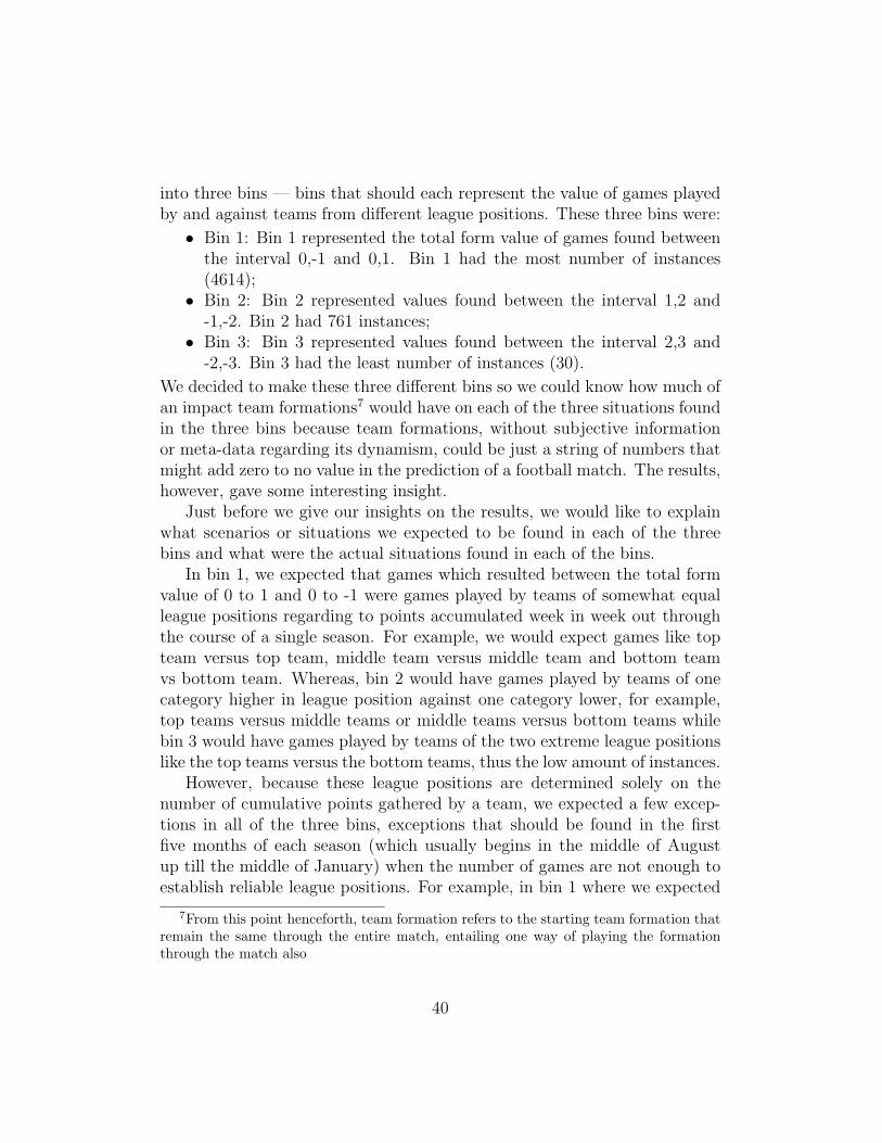
We decided to make these three different bins so we could know how much ofan impact team formations7 would have on each of the three situations foundin the three bins because team formations, without subjective informationor meta-data regarding its dynamism, could be just a string of numbers thatmight add zero to no value in the prediction of a football match. The results,however, gave some interesting insight.

Just before we give our insights on the results, we would like to explainwhat scenarios or situations we expected to be found in each of the threebins and what were the actual situations found in each of the bins.

In bin 1, we expected that games which resulted between the total formvalue of 0 to 1 and 0 to -1 were games played by teams of somewhat equalleague positions regarding to points accumulated week in week out throughthe course of a single season. For example, we would expect games like topteam versus top team, middle team versus middle team and bottom teamvs bottom team. Whereas, bin 2 would have games played by teams of onecategory higher in league position against one category lower, for example,top teams versus middle teams or middle teams versus bottom teams whilebin 3 would have games played by teams of the two extreme league positionslike the top teams versus the bottom teams, thus the low amount of instances.

However, because these league positions are determined solely on thenumber of cumulative points gathered by a team, we expected a few excep-tions in all of the three bins, exceptions that should be found in the firstfive months of each season (which usually begins in the middle of Augustup till the middle of January) when the number of games are not enough toestablish reliable league positions. For example, in bin 1 where we expected

7From this point henceforth, team formation refers to the starting team formation thatremain the same through the entire match, entailing one way of playing the formationthrough the match also

40

games played by teams of equal league positions, we found exceptions likethe game played between Burnley and Manchester United on the 30th ofAugust, 2014, a bottom league team against a top league team game; orthe game played against Inter Milan and Sassuolo on the 14th of September,2014, a top league team against a middle league team; of course there weremany other instances found like this which most of them were played in thefirst five months of the season with not enough games to establish reliableleague positions. Also in bin 2, we found exceptions like the game playedagainst Bayern Munich and Dortmund on the 1st of November, 2014, whichis a game played between teams of equal league positions; or the game playedbetween Reading and Chelsea on the 30th of January, 2013, a bottom leagueteam against a top league team. Finally, in bin 3, because of the rare case ofteams getting the values between 2 to 3 and -2 to -3, we expected two things,that:

• the number of instances will be the least amongst the three bins and;• as mentioned earlier, it would be a representative of games played

between the top league teams and the bottom league teams.

Eventually, yes the number of instances was the least compared to the otherbins but the latter was not so. The instances found in bin 3 were not rep-resentative of games played between the top and the bottom league teamsalone but rather games played only in the first five months of the seasons.This eventual discovery became the deciding factor on how good and easythe prediction on bin 3 should have been and what it actually was.

The results shown in Figures 14 and 15 show the difference in accuracylevels with and without the inclusion of formations in each of the three bins.In bins 1 and 2, the accuracy remained more or less the same after theinclusion of team formations. In bin 1, the accuracy levels, both with andwithout the team formations are above the default accuracy of 45.57% butstill not a good enough accuracy which entailed that instances in bin 1 aredifficult to predict with or without the inclusion of team formations. Whilein bin 2 the accuracy levels, both with and without the inclusion of theteam formations are about 20% more than the default accuracy, which wasexpected because of the type of games that are represented in bin 2. However,the inclusion of the team formations in both bins 1 and 2 had little or noeffect, this could mean that matches played in these two bins are more likelyto change formations during the course of a game or change how the formationis played during the course of the game through substitutions or coaching

41

instructions.Whereas, in bin 3, although both the accuracy levels were below the

default accuracy meaning the prediction in this bin was very poor, therewas about a four percent (4%) increase in accuracy level with the inclusionof team formations. We would expect the poorness of the prediction to beas a result of the low amount of instances used but as we showed in thelearning curve in Figure 30, the accuracy level remains more or less thesame regardless of the amount of instances in regards to this research. As wecrossed out the number of instances being the reason for the poor predictions,we looked into what this bin was representative of and attributed the poorresults to the fact that, unlike in bins 1 and 2 where the instances consistedof games that were played through the course of the entire seasons, all ofthe instances in bin 3 consisted of games played only in the first five monthsof the seasons, making the dataset very shallow in terms of the algorithmseeing a good enough picture to predict with. However, regardless of the pooraccuracy results, the inclusion of team formations resulted in a four percent(4%) increase which could mean that teams do not change their formationsor how the formations are played early on in the season as this bin consistsof games played in the first five months of the seasons. Whereas, as theseason progresses, teams change their formations or how their formations areplayed.

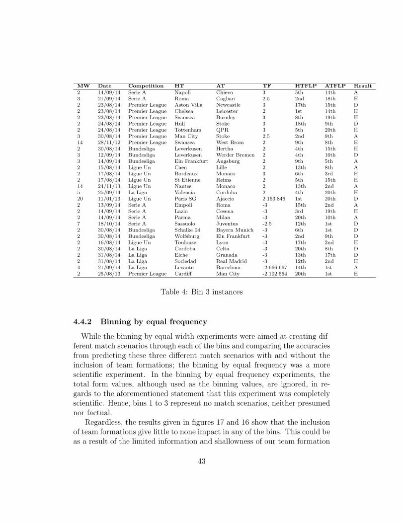
Below is a table showing the instances found in bin 3; the table alsoincludes the final league position of both the home (HTFLP) and awayteams (ATFLP) and the match-week8 (MW) of each game played, as wellas the result (R)of the game, the competition name, date of the match, home(HT) and away (AT) team names and total form (TF) value of each match.This table shows two things mentioned earlier regarding bin 3, that:

• bin three is representative of games played within the first and fifthmonths of the season and;

• bin three can not be said to be representative of games played betweenthe top league teams and the bottom league teams

8The Bundesliga has 34 match-weeks while the other four leagues have 38 match-weeks

42

MW Date Competition HT AT TF HTFLP ATFLP Result

2 14/09/14 Serie A Napoli Chievo 3 5th 14th A3 21/09/14 Serie A Roma Cagliari 2.5 2nd 18th H2 23/08/14 Premier League Aston Villa Newcastle 3 17th 15th D2 23/08/14 Premier League Chelsea Leicester 2 1st 14th H2 23/08/14 Premier League Swansea Burnley 3 8th 19th H2 24/08/14 Premier League Hull Stoke 3 18th 9th D2 24/08/14 Premier League Tottenham QPR 3 5th 20th H3 30/08/14 Premier League Man City Stoke 2.5 2nd 9th A14 28/11/12 Premier League Swansea West Brom 2 9th 8th H2 30/08/14 Bundesliga Leverkusen Hertha 2 4th 15th H3 12/09/14 Bundesliga Leverkusen Werder Bremen 2 4th 10th D3 14/09/14 Bundesliga Ein Frankfurt Augsburg 2 9th 5th A2 15/08/14 Ligue Un Caen Lille 2 13th 8th A2 17/08/14 Ligue Un Bordeaux Monaco 3 6th 3rd H2 17/08/14 Ligue Un St Etienne Reims 2 5th 15th H14 24/11/13 Ligue Un Nantes Monaco 2 13th 2nd A5 25/09/14 La Liga Valencia Cordoba 2 4th 20th H20 11/01/13 Ligue Un Paris SG Ajaccio 2.153.846 1st 20th D2 13/09/14 Serie A Empoli Roma -3 15th 2nd A2 14/09/14 Serie A Lazio Cesena -3 3rd 19th H2 14/09/14 Serie A Parma Milan -3 20th 10th A7 18/10/14 Serie A Sassuolo Juventus -2.5 12th 1st D2 30/08/14 Bundesliga Schalke 04 Bayern Munich -3 6th 1st D2 30/08/14 Bundesliga Wolfsburg Ein Frankfurt -3 2nd 9th D2 16/08/14 Ligue Un Toulouse Lyon -3 17th 2nd H2 30/08/14 La Liga Cordoba Celta -3 20th 8th D2 31/08/14 La Liga Elche Granada -3 13th 17th D2 31/08/14 La Liga Sociedad Real Madrid -3 12th 2nd H4 21/09/14 La Liga Levante Barcelona -2.666.667 14th 1st A2 25/08/13 Premier League Cardiff Man City -2.102.564 20th 1st H

Table 4: Bin 3 instances

4.4.2 Binning by equal frequency

While the binning by equal width experiments were aimed at creating dif-ferent match scenarios through each of the bins and comparing the accuraciesfrom predicting these three different match scenarios with and without theinclusion of team formations; the binning by equal frequency was a morescientific experiment. In the binning by equal frequency experiments, thetotal form values, although used as the binning values, are ignored, in re-gards to the aforementioned statement that this experiment was completelyscientific. Hence, bins 1 to 3 represent no match scenarios, neither presumednor factual.

Regardless, the results given in figures 17 and 16 show that the inclusionof team formations give little to none impact in any of the bins. This could beas a result of the limited information and shallowness of our team formation

43

data. It could also mean that randomly selecting a match is not the most idealwhen making predictions with team formations, making match scenarios, asis done in the binning by equal width experiments, gives more insight andadded advantage on what to expect when making predictions with teamformations.

4.5 Formation Clustering

In the attempts to reduce the number of unique team formations we had inour dataset from 20, we clustered the team formations using the hierarchicalclustering method. We clustered the formations for the same reason wepartitioned the formations in the team formation experiments, because outof the 20 team formations, 13 of them were used by less than 10% of thedataset, while of that 13, 4 were used by less than 1% of the dataset.

Although, the team formations had already been partitioned as shown inTable 6, the partitioned formations shown in the table did not achieve themain objective which was to reduce the number of total team formations usedby less than 1% of the dataset. Moreover, partitioning the team formations,as shown in the table mentioned above, was based on little expert knowledge.Factors like:

• how easy would it be to change to any of the formations partitionedtogether?

• how comparable in playing styles are the formations partitioned to-gether?

were taken into consideration while partitioning similar team formations to-gether.

We decided to partition the team formations in a more scientific approach,through clustering — hierarchical clustering. These formations (clustered)were based on 1) shots, and 2) shots on target. Both shots and shots ontarget based clusters produced interesting results as shown in their respectivedendrograms. The primary objectives for clustering the team formations wereto 1) scientifically, partition the team formations based on historic data andfeature selection and 2) to the aim of having a bigger impact than the teamformations partitioned based on expert knowledge when included in makingpredictions.

One of the two objectives mentioned earlier was more successful than theother. The formations were clustered based on feature selection, in our case,

44

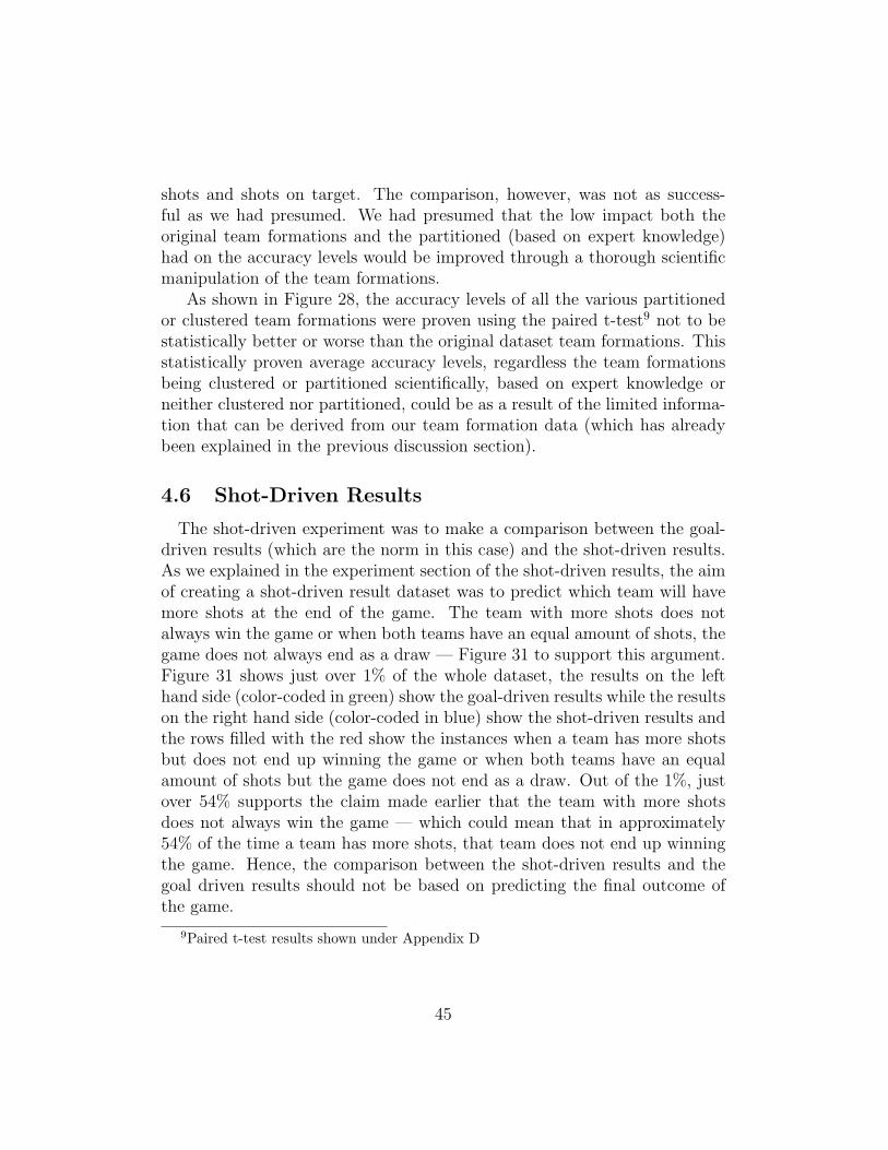
shots and shots on target. The comparison, however, was not as success-ful as we had presumed. We had presumed that the low impact both theoriginal team formations and the partitioned (based on expert knowledge)had on the accuracy levels would be improved through a thorough scientificmanipulation of the team formations.

As shown in Figure 28, the accuracy levels of all the various partitionedor clustered team formations were proven using the paired t-test9 not to bestatistically better or worse than the original dataset team formations. Thisstatistically proven average accuracy levels, regardless the team formationsbeing clustered or partitioned scientifically, based on expert knowledge orneither clustered nor partitioned, could be as a result of the limited informa-tion that can be derived from our team formation data (which has alreadybeen explained in the previous discussion section).

4.6 Shot-Driven Results

The shot-driven experiment was to make a comparison between the goal-driven results (which are the norm in this case) and the shot-driven results.As we explained in the experiment section of the shot-driven results, the aimof creating a shot-driven result dataset was to predict which team will havemore shots at the end of the game. The team with more shots does notalways win the game or when both teams have an equal amount of shots, thegame does not always end as a draw — Figure 31 to support this argument.Figure 31 shows just over 1% of the whole dataset, the results on the lefthand side (color-coded in green) show the goal-driven results while the resultson the right hand side (color-coded in blue) show the shot-driven results andthe rows filled with the red show the instances when a team has more shotsbut does not end up winning the game or when both teams have an equalamount of shots but the game does not end as a draw. Out of the 1%, justover 54% supports the claim made earlier that the team with more shotsdoes not always win the game — which could mean that in approximately54% of the time a team has more shots, that team does not end up winningthe game. Hence, the comparison between the shot-driven results and thegoal driven results should not be based on predicting the final outcome ofthe game.

9Paired t-test results shown under Appendix D

45

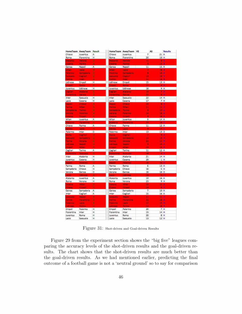
Figure 31: Shot-driven and Goal-driven Results

Figure 29 from the experiment section shows the “big five” leagues com-paring the accuracy levels of the shot-driven results and the goal-driven re-sults. The chart shows that the shot-driven results are much better thanthe goal-driven results. As we had mentioned earlier, predicting the finaloutcome of a football game is not a ‘neutral ground’ so to say for comparison

46

between the shot-driven results and goal-driven results because goal-drivenresults are a 100% accurate regarding if a team has more goals, will alwaysend up winning the game, whereas, it is not the same for the shot-drivenresults.

5 CONCLUSION & FUTURE WORK

This thesis paper was set out to show a comparison between differentmethods a football match can be predicted using feature selection, whetheror not team formations add value in predicting a football match, what fea-tures would perform better than the others, what combination of featuresare best used together and their overall performances in predicting footballmatches. The general theoretical literature regarding football match predic-tions propose one method for predicting football games using quantitativedata, qualitative data or a mixture of both, whichever type of data is used,a comparison of different methods and the use of team formations as a de-pendent feature to predict a football match is a gap usually left unanswered.This thesis paper sought to answer these two questions:

1. Which features or combination of features would produce better pre-dictions?

2. Do team formations add significant value to football match predic-tions?

5.1 Conclusion

The results shown in this thesis paper show that:

• Using the total team forms produce better results compared to usinga defined n form value;

• The total form, which could be equivalent to a team’s league positionor team strength is a good baseline feature for making predictions;

• Quantitative data like shots, shots on target, goals, goals ratio andshots ratio used in this paper produce similar results;

• Team formations — as just a string of numbers did not show to be ofadded value in making predictions;

• Clustering team formations based on historic data like shots, shots ontarget or goals do not produce realistic team formation clusters whichcould suggest the complexities that could be found in team formation.

47

The importance of football data in the world today is ever increasing, forthis reason, conducting research in the area of sports data analysis is only asgood as the data you can get your hands on. This, for us was a limitationencountered and need s to be considered in this research. Despite this limita-tion, we have been able to provide, using the data we had, insight regardingthe research questions we posed at the beginning of this thesis paper.

5.2 Future Work

Team formations have shown to be as complex as the game of footballitself, in the sense that team formations on its own has a number of otherfactors that influence how they are executed. For example, substitutionscould affect how a team formation is played, injuries, player availability,team more, fatigue and so many more. If team formations are to become anindependent feature in football match prediction, they need to be defined asa combination of other mini-factors like the factors mentioned earlier.

Based on our results, it is also recommendable to say that a mixtureof qualitative data with quantitative data, which, according to general lit-erature, has shown to always give better results, would produce a bettercomparison of methods for predicting a football match.

48

A

A description of Dataset

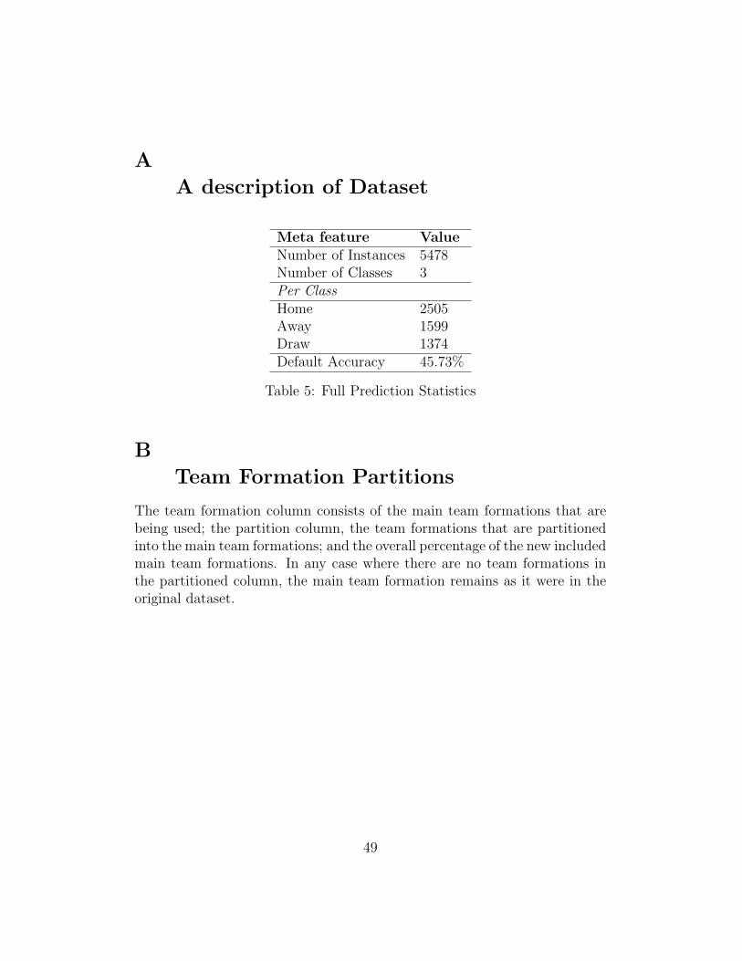
Meta feature ValueNumber of Instances 5478Number of Classes 3Per ClassHome 2505Away 1599Draw 1374Default Accuracy 45.73%

Table 5: Full Prediction Statistics

B

Team Formation Partitions

The team formation column consists of the main team formations that arebeing used; the partition column, the team formations that are partitionedinto the main team formations; and the overall percentage of the new includedmain team formations. In any case where there are no team formations inthe partitioned column, the main team formation remains as it were in theoriginal dataset.

49

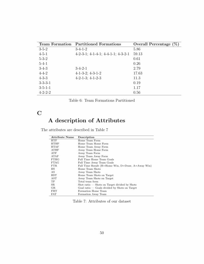
Team Formation Partitioned Formations Overall Percentage (%)3-5-2 3-4-1-2 5.864-5-1 4-2-3-1; 4-1-4-1; 4-4-1-1; 4-3-2-1 59.135-3-2 0.615-4-1 0.263-4-3 3-4-2-1 2.794-4-2 4-1-3-2; 4-3-1-2 17.634-3-3 4-2-1-3; 4-1-2-3 11.33-3-3-1 0.193-5-1-1 1.174-2-2-2 0.56

Table 6: Team Formations Partitioned

C

A description of Attributes

The attributes are described in Table 7

Attribute Name Description

HTF Home Team FormHTHF Home Team Home FormHTAF Home Team Away FormATHF Away Team Home FormATF Away Team FormATAF Away Team Away FormFTHG Full Time Home Team GoalsFTAG Full Time Away Team GoalsFTR Full Time Result (H=Home Win, D=Draw, A=Away Win)HS Home Team ShotsAS Away Team ShotsHST Home Team Shots on TargetAST Away Team Shots on TargetTF Total team formSR Shot ratio — Shots on Target divided by ShotsGR Goal ratio — Goals divided by Shots on TargetFHT Formation Home TeamFAT Formation Away Team

Table 7: Attributes of our dataset

50

D

Paired T-test Results

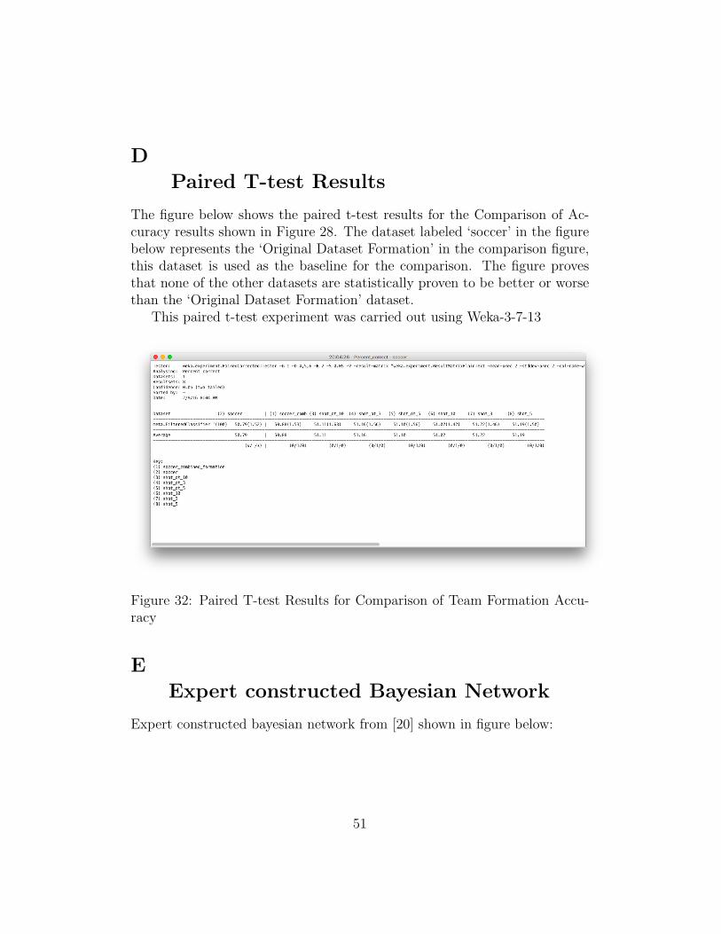
The figure below shows the paired t-test results for the Comparison of Ac-curacy results shown in Figure 28. The dataset labeled ‘soccer’ in the figurebelow represents the ‘Original Dataset Formation’ in the comparison figure,this dataset is used as the baseline for the comparison. The figure provesthat none of the other datasets are statistically proven to be better or worsethan the ‘Original Dataset Formation’ dataset.

This paired t-test experiment was carried out using Weka-3-7-13

Figure 32: Paired T-test Results for Comparison of Team Formation Accu-racy

E

Expert constructed Bayesian Network

Expert constructed bayesian network from [20] shown in figure below:

51

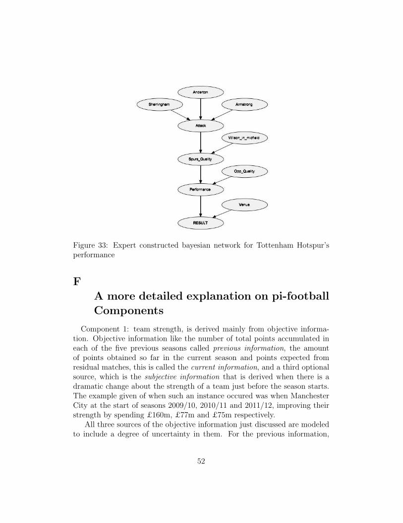
Figure 33: Expert constructed bayesian network for Tottenham Hotspur’sperformance

F

A more detailed explanation on pi-football

Components

Component 1: team strength, is derived mainly from objective informa-tion. Objective information like the number of total points accumulated ineach of the five previous seasons called previous information, the amountof points obtained so far in the current season and points expected fromresidual matches, this is called the current information, and a third optionalsource, which is the subjective information that is derived when there is adramatic change about the strength of a team just before the season starts.The example given of when such an instance occured was when ManchesterCity at the start of seasons 2009/10, 2010/11 and 2011/12, improving theirstrength by spending £160m, £77m and £75m respectively.

All three sources of the objective information just discussed are modeledto include a degree of uncertainty in them. For the previous information,

52

the information becomes less important for each previous season, while thecurrent information becomes more important after each successive match-week, and finally, the optional subjective information, this importance of thisinformation is dependent on the degree of the expert’s confidence regardinghis/her indications. A high confidence breeds lower uncertainties, as a lowconfidence, higher uncertainties.

The subsequent components are mainly dependent on expert subjectiveinformation.

Component 2: team form, generates the team’s recent performance whichis the difference between the expected performance — represented by whatthe model had initially forecasted and its real performance during the fivemost recent match-weeks; this difference is then represented on a scale from0 to 1, a value closer to 0.5 indicates the team’s performing as expected andabove 0.5 indicates performing higher than expected. Home advantage isalso taken into consideration by assigning a heavier weight on home ‘forms’.When this form has been generated, it is then revised according to subjectiveindications about the availability of certain players. These certain player (s)are categorized into (i) Primary key-player availability, (ii) secondary key-player availability, (iii) tertiary key-player availability(iv) remaining firstteam players availability and (v) first team returning players. The availabilityof these certain players, again are measured with the confidence levels of theexpertise about the impact they can have on the outcome of the game.

Component 3: psychological impact, is indicated in two levels: level oneis derived from the teams’ head to head bias and the managerial impact; leveltwo is generated from the teams’ confidence, spirit and motivation level. Theinformation accessed in level one is updated by that of level two, for bothteams and regarded as the teams’ psychological impact. These indicationsgotten from the experts are also limited to a degree of uncertainty.

Component 4: team fatigue, is determined by the toughness or difficultyof the previous match, the number of days gap since that match, the numberof rested first team players (if any) and the number of first team playersthat have participated in international matches (if any). This component isalso divided into two stages, these are: Stage 1 and Stage 2. Stage 1 is acombination of a ‘restness’ micro stage which consists of the number of dayssince last match and the number of first team players rested during the lastmatch; and the toughness or difficulty of the previous match. This first stageis then updated in the second stage, as is done in the psychological impactcomponent. The information in the second stage is gotten from national

53

team participation (if any).

54

References

[1] Naomi S Altman. An introduction to kernel and nearest-neighbor non-parametric regression. The American Statistician, 46(3):175–185

[2] V Barnett and S Hilditch. The effect of an artificial pitch surface on hometeam performance in football (soccer). Journal of the Royal StatisticalSociety. Series A (Statistics in Society), pages 39–50

[3] Carl Bialik. The people tracking every touch, pass and tackle inthe world cup. http://fivethirtyeight.com/features/the-people-tracking-every-touch-pass-and-tackle-in-the-world-cup/.

[4] AG Biichner, Werner Dubitzky, Alfons Schuster, Philippe Lopes,PG O’Doneghue, John G Hughes, David A Bell, Kenneth Adamson,John A White, and John MCC Anderson. Corporate evidential decisionmaking in performance prediction domains. Morgan Kaufmann Publish-ers Inc., 1997.

[5] Leo Breiman. Random forests. Machine learning, 45(1):5–32

[6] Joseph Buchdahl. Fixed odds sports betting. High Stakes, 2003.

[7] Anthony C Constantinou, Norman E Fenton, and Martin Neil. pi-football: A bayesian network model for forecasting association footballmatch outcomes. Knowledge-Based Systems, 36:322–339

[8] Alexis Direr. Are betting markets efficient? evidence from europeanfootball championships. Applied Economics, 45(3):343–356

[9] Mark J Dixon and Stuart G Coles. Modelling association football scoresand inefficiencies in the football betting market. Journal of the RoyalStatistical Society: Series C (Applied Statistics), 46(2):265–280

[10] Arpad E The rating of chessplayers, past and present. Arco Pub., 1978.

[11] Football-Data. Football results, statistics and soccer betting odds data.http://football-data.co.uk/.

[12] Football-Lineups. Football lineups, tactics, transfers, injuries and tour-nament data. http://www.football-lineups.com.

55

[13] David Forrest, John Goddard, and Robert Simmons. Odds-setters asforecasters: The case of english football. International Journal of Fore-casting, 21(3):551–564 0169–2070, 2005.

[14] David Forrest and Robert Simmons. Globalisation and efficiency in thefixed-odds soccer betting market. University of Salford, Centre for theStudy of Gambling and Commercial Gaming, 2001.

[15] Yoav Freund and Robert E Schapire. Experiments with a new boostingalgorithm, volume 96. 1996.

[16] John Goddard and Ioannis Asimakopoulos. Forecasting football resultsand the efficiency of fixedodds betting. Journal of Forecasting, 23(1):51–66

[17] John Goddard and Ioannis Asimakopoulos. Forecasting football resultsand the efficiency of fixedodds betting. Journal of Forecasting, 23(1):51–66

[18] Lars Magnus Hvattum and Halvard Arntzen. Using elo ratings for matchresult prediction in association football. International Journal of fore-casting, 26(3):460–470 0169–2070, 2010.

[19] Investopedia. Poisson distribution. http://www.investopedia.com/terms/p/poisson-distribution.asp.

[20] A Joseph, Norman E Fenton, and Martin Neil. Predicting football resultsusing bayesian nets and other machine learning techniques. Knowledge-Based Systems, 19(7):544–553

[21] Tim Kuypers. Information and efficiency: an empirical study of a fixedodds betting market. Applied Economics, 32(11):1353–1363

[22] Alan J Lee. Modeling scores in the premier league: is manchester unitedreally the best? Chance, 10(1):15–19

[23] Christoph Leitner, Achim Zeileis, and Kurt Hornik. Forecasting sportstournaments by ratings of (prob) abilities: A comparison for the euro2008. International Journal of Forecasting, 26(3):471–481 0169–2070,2010.

56

[24] Mike J Maher. Modelling association football scores. Statistica Neer-landica, 36(3):109–118

[25] M Moroney. Facts from figures. Penguin, 1951.

[26] Alan M Nevill, Sue M Newell, and Sally Gale. Factors associated withhome advantage in english and scottish soccer matches. Journal of SportsSciences, 14(2):181–186

[27] Paul Nicholson. Stats swoop to add prozone to its growing globalpower play. http://www.insideworldfootball.com/world-football/42-news/16956-stats-swoops-to-add-prozone-to-its-growing-global-power-play.

[28] Richard Pollard. Evidence of a reduced home advantage when a teammoves to a new stadium. Journal of Sports Sciences, 20(12):969–9732002.

[29] J Ross Quinlan. C4. 5: Programming for machine learning. MorganKauffmann, 1993.

[30] C Reep, R Pollard, and B Benjamin. Skill and chance in ball games.Journal of the Royal Statistical Society. Series A (General), pages 623–629

[31] Alexander P Rotshtein, Morton Posner, and AB Rakityanskaya. Foot-ball predictions based on a fuzzy model with genetic and neural tuning.Cybernetics and Systems Analysis, 41(4):619–630 2005.

[32] N. J. A. Sloane. Bell or exponential numbers: number of ways to parti-tion a set of n labeled elements. https://oeis.org/A000110.

[33] Koya Suzuki and Kazunobu Ohmori. Effectiveness of fifa/coca-colaworld ranking in predicting the results of fifa world cuptm finals. 2008.

[34] Mark Thompson. On any given sunday: Fair competitor orderings withmaximum likelihood methods. Journal of the American Statistical As-sociation, 70(351a):536–541

[35] A Tsakonas, G Dounias, S Shtovba, and V Vivdyuk. Soft computing-based result prediction of football games. Citeseer, 2002.

57

[36] Guido Van Rossum. An introduction to python for unix/c programmers.Proc. of the NLUUG najaarsconferentie. Dutch UNIX users group, 1993.

[37] Ian H Witten and Eibe Data Mining: Practical machine learning toolsand techniques. Morgan Kaufmann, 2005.

58