Auton Robot (2007) 23: 97–111DOI 10.1007/s10514-007-9034-y

A comparison of line extraction algorithms using 2D rangedata for indoor mobile robotics

Viet Nguyen · Stefan Gächter · Agostino Martinelli ·Nicola Tomatis · Roland Siegwart

Received: 21 September 2006 / Revised: 14 March 2007 / Accepted: 28 March 2007 / Published online: 8 June 2007© Springer Science+Business Media, LLC 2007

Abstract This paper presents an experimental evaluation ofdifferent line extraction algorithms applied to 2D laser scansfor indoor environments. Six popular algorithms in mobilerobotics and computer vision are selected and tested. Realscan data collected from two office environments by us-ing different platforms are used in the experiments in or-der to evaluate the algorithms. Several comparison criteriaare proposed and discussed to highlight the advantages anddrawbacks of each algorithm, including speed, complexity,correctness and precision. The results of the algorithms arecompared with ground truth using standard statistical meth-ods. An extended case study is performed to further evaluatethe algorithms in a SLAM application.

Keywords Line extraction algorithm · 2D range data ·Mobile robotics

V. Nguyen (�) · S. Gächter · A. Martinelli · R. SiegwartAutonomous Systems Laboratory (ASL), Swiss Federal Instituteof Technology Zürich (ETHZ), Tannenstrasse 3, 8092 Zurich,Switzerlande-mail: viet.nguyen@mavt.ethz.ch

S. Gächtere-mail: stefan.gaechter@mavt.ethz.ch

A. Martinellie-mail: agostino.martinelli@mavt.ethz.ch

R. Siegwarte-mail: rsiegwart@ethz.ch

N. TomatisBlueBotics SA, PSE-C, 1015 Lausanne, Switzerlande-mail: nicola.tomatis@bluebotics.com

1 Introduction

It is important for a mobile robot to be able to autonomouslynavigate and localize itself in a known or unknown en-vironment. A precise position estimation always serves asthe heart in any navigation systems, such as localization,map building or path planning. It is well known that puredead-reckoning methods, e.g. odometry, are prone to errorsthat grow unbounded over time (Iyengar and Elfes 1991).The problem gives rise to a variety of solutions using dif-ferent exteroceptive sensors (sonar, infrared, laser, vision,etc.). Among different types of sensors, 2D laser range find-ers are becoming increasingly popular in mobile robotics.For example, laser scanners have been used in localiza-tion (Cox 1991; Jensfelt and Christensen 1998), dynamicmap building (Lu and Milios 1994; Gutmann et al. 1998;Castellanos and Tardós 1996; Tomatis et al. 2003) or featuretracking (e.g. for collision avoidance) (Pears 2000). Thereare many advantages of laser scanners compared to othersensors: they provide dense and more accurate range mea-surements, they have high sampling rates, high angular res-olution, good range distance and resolution.

One primary issue is how to accurately match sensed dataagainst information in a priori map or information that hasbeen continuously collected. There are two common match-ing techniques that have been used in mobile robotics: point-based matching and feature-based matching. The early workof Cox (1991) uses range data to help the robot localizing it-self in a small polygonal environment. He proposes a match-ing algorithm between point images and target models ina priori map using an iterative least-squares minimizationmethod. Another work done by Lu and Milios (1994) ad-dresses the problem of self-localization in an unknown envi-ronment, not necessarily polygonal. The proposed approachis to approximate the alignment of two consecutive scans

98 Auton Robot (2007) 23: 97–111

and then iteratively improve the alignment by defining andminimizing some distance between the scans.

Instead of working directly with raw measurement points,feature-based matching first transforms the raw scans intogeometric features. The extracted features are then used formatching in the next step. This approach has been stud-ied and employed intensively in recent research on fea-ture extraction, feature tracking, robot localization, dynamicmap building, etc. (Crowley 1985; Leonard et al. 1992;Castellanos and Tardós 1996; Gutmann and Schlegel 1996;Jensfelt and Christensen 1998; Schröter et al. 2002; Brun-skill and Roy 2005). Being more compact, they requiremuch less memory and still provide rich and accurate infor-mation. Algorithms based on parameterized geometric fea-tures are therefore more efficient compared to point-basedalgorithms.

Among many geometric primitives, line segments are thesimplest ones. It is easy to describe most office environmentusing line segments. Many algorithms have been proposedfor mobile robotics using line features extracted from 2Drange data. Castellanos and Tardós (1996) propose a linesegmentation method inspired from an algorithm in com-puter vision, used with a priori map as an approach to ro-bot localization. Vandorpe et al. (1996) introduce a dynamicmap building algorithm based on geometrical features, e.g.lines and circles, using a laser scanner. Arras and Siegwart(1997) use a 2D scan segmentation method based on line re-gression in map-based localization. Jensfelt and Christensen(1998) present a technique for acquisition and tracking ofthe pose of a mobile robot in an office environment witha laser scanner by extracting orthogonal lines (walls). Pfis-ter et al. (2003) suggest a line extraction algorithm usingweighted line fitting for line-based map building. Finally,Brunskill and Roy (2005) propose an incremental proba-bilistic technique to extract segments for solving the SLAMproblem.

Many work has been done on line extraction. However,there is a lack of comprehensive comparisons of the so farproposed algorithms. Selecting the best method to extractlines from scan data is the first task for anyone who is go-ing to build a line-based navigation system using 2D laserscanners. In terms of speed, one would prefer the fastest al-gorithm for his real time application. In terms of quality, badline extraction can seriously lead the system to divergence inline-based SLAM. Implementation complexity is also one ofthe main aspects to take into account.

The work done by Gutmann and Schlegel (1996) givesa brief comparison of three algorithms which are relativelyout of date compared to ones found in recent research. More-over, the uncertainty modeling of the used parameters is notintroduced in their paper. Borges and Aldon (2004) presentan extended version of split-and-merge and compare theirmethod with a generic split-and-merge algorithm and a line

tracking (incremental) algorithm. Sack and Burgard (2004)perform a comparison of three selected algorithms on rangedata. However, in both papers the evaluation results are in-directly observed and interpreted from the map built by themapping process. A direct comparison of the extracted linesby the selected algorithms using probabilistic analysis is stillmissing.

This paper presents a throughout evaluation of six lineextraction algorithms applied to laser range scans. Thiswork is an extension of the one described in (Nguyen etal. 2005). The six selected algorithms are the most com-monly used in mobile robotics and computer vision. Sev-eral comparison criteria are proposed and discussed, includ-ing speed, complexity, correctness and precision. The ex-periments are performed on two datasets collected from theAutonomous Systems Laboratory—EPFL, Switzerland andthe Intel Jones Farms Campus, Oregon with the environmentsize of 80 m × 50 m and 40 m × 40 m, respectively. The re-sults of the algorithms are compared with ground truth usingstandard statistical methods. One case study is performed toevaluate the maps obtained from a SLAM application whenusing different line extraction algorithms. Finally, the con-clusions are presented.

2 Problem statement

A range scan describes a 2D slice of the environment. Pointsof a range scan are specified in polar coordinate system(ρi, θi) whose origin is the location of the sensor (or the ro-bot location offset by the mounting distance). It is commonto assume that the noise on range measurement follows aGaussian distribution with zero mean and variance σ 2

ρi. We

neglect the small angular uncertainty for the ease of com-puting the covariance matrix of line parameters (see Arrasand Siegwart 1997 for more derivation detail). Note that inthis work, we focus on the performance of the algorithms.We do not consider systematic errors as they mainly dependon a specific hardware and testing environment (Diosi andKleeman 2003a, 2003b).

We choose the polar form to represent a line model:

x cosα + y sinα = r

where −π < α ≤ π is the angle between the x axis and thenormal of the line; r ≥ 0 is the perpendicular distance ofthe line to the origin; (x, y) is the Cartesian coordinates of apoint on the line.

The covariance matrix of line parameters is:

cov(r,α) =[

σ 2r σrα

σrα σ 2α

].

There are three main problems in line extraction in anunknown environment (Forsyth and Ponce 2003). They are:

Auton Robot (2007) 23: 97–111 99

• How many lines are there?• Which points belong to which line?• Given the points that belong to a line, how to estimate the

line model parameters?

In implementing the algorithms, we try to use as manycommon routines as possible, so that the experimental re-sults reflect mainly the differences of the algorithmic con-cepts. Particularly for the third problem, we use a commonfitting method, called total-least-squares, for all the algo-rithms since it has been used extensively in the literature(Arras and Siegwart 1997; Jensfelt and Christensen 1998;Einsele 1997; Lu and Milios 1994; Siadat et al. 1997).Hence, the algorithms differ only in solving the first twoproblems. Regarding the parameter settings, we define 2 setsof parameters. The first set consists of parameters of inputdata (e.g. number of points per scan), the sensor model (e.g.sensor uncertainties), desired output (e.g. minimal length ofa line segment, maximal uncertainty) and parameters for thecommon routines (e.g. clustering, merging functions). Theseparameters are set to the same values for all the algorithms.The second set consists of specific parameter values for in-dividual algorithm procedure. These parameters are chosenindividually for each algorithm based on experimental tun-ning so that the best performance is obtained among severalruns.

Notice that with high frequency of the up-to-date laserrange finders (up to 75 Hz for a SICK LMS 200), we assumethat the scans are obtained in batches (half or full scanningcycle). We make also the assumption that the effect of therobot motion on individual scan points (in one batch) is neg-ligible. This however holds only when the robot translationand rotation speeds are small, e.g. few meters per second.For outdoor navigation, one might have to revise this as-sumption.

3 Selected algorithms and related work

This section briefly presents the concepts of the six selectedline extraction algorithms. Our selection is based on theirperformance and popularity in both mobile robotics andcomputer vision. Only basic versions of the algorithms aresummarized even though the details may vary in differentimplementations and applications. Interested reader shouldrefer to the indicated references for more details. Our imple-mentation follows closely the pseudo-code described belowwhen not stated otherwise.

3.1 Split-and-merge algorithm

Split-and-Merge is probably the most popular line extractionalgorithm which originates from computer vision in 1974by Pavlidis and Horowitz (1974). It has been studied and

used in many robotic research (Castellanos and Tardós 1996;Einsele 1997; Siadat et al. 1997; Borges and Aldon 2004;Zhang and Ghosh 2000).

Algorithm 1: Split-and-Merge

1 Initial: set s1 consists of N points. Put s1 in a list L2 Fit a line to the next set si in L3 Detect point P with maximum distance dP to the line4 If dP is less than a threshold, continue (go to 2)5 Otherwise, split si at P into si1 and si2, replace si in L

by si1 and si2, continue (go to 2)6 When all sets (segments) in L have been checked, merge

collinear segments.

In the implementation, we make a small modification toline 3 so that we search for a splitting position where twoadjacent points P1 and P2 are at the same side to the lineand both have distances to the line greater than the thresh-old (if only 1 such point is found, it is ignored as a noisypoint). Intuitively, we should split at a point that has locallymaximal distance to the line. Notice that in line 2, we use aleast-squares method for line fitting.

One can implement the algorithm differently so that aline is constructed simply by connecting the first and thelast points. In this case, the algorithm is called Iterative-End-Point-Fit as in (Duda and Hart 1973; Siadat et al. 1997;Borges and Aldon 2004; Zhang and Ghosh 2000).

3.2 Incremental algorithm

Simplicity is the main advantage of this algorithm. It hasbeen used in many applications (Forsyth and Ponce 2003;Vandorpe et al. 1996; Taylor and Probert 1996) and is alsoknown as Line-Tracking (Siadat et al. 1997).

Algorithm 2: Incremental

1 Start by the first 2 points, construct a line2 Add the next point to the current line model3 Recompute the line parameters4 If it satisfies a condition, continue (go to 2)5 Otherwise, put back the last point, recompute the line pa-

rameters, return the line6 Continue with the next 2 points, go to 2

In the implementation, we add 5 measurement points ateach step (line 2) to speed up the incremental process. Whenthe line does not satisfy a predefined line condition (vari-ances of line parameters are less than some thresholds), thelast 5 points are put back and the algorithm is switched backto the normal mode (adding one measurement point at atime). Again, we use a total-least-squares method for linefitting (line 3, 5).

The incremental scheme has been used in the algorithmsproposed in (Adams and Kerstens 1998) and (Pears 2000),

100 Auton Robot (2007) 23: 97–111

however they use the EKF to estimate the parameters ofextracted lines which is equivalent to using the total-least-squares fitting in this paper.

3.3 Hough transform algorithm

Hough Transform tends to be most successfully applied toline finding in intensity images (Forsyth and Ponce 2003). Ithas been brought in to robotics for extracting line from scanimages (Forsberg et al. 1995; Jensfelt and Christensen 1998;Iocchi and Nardi 2002; Pfister et al. 2003).

Algorithm 3: Hough-Transform

1 Initial: A set of N points2 Initialize the accumulator array3 Construct values for the array4 Choose the element with max. votes Vmax

5 If Vmax is less than a threshold, terminate6 Otherwise, determine the inliers7 Fit a line through the inliers and store the line8 Remove the inliers from the set, goto 2

There are some drawbacks with Hough Transform:

• It is usually difficult to choose an appropriate grid size forthe accumulator array.

• Basic Hough Transform algorithm does not take noise anduncertainty into account when estimating the line parame-ters.

In this implementation, we use a resolution of 1 cm and0.4° as the grid size of range and angle, respectively. Toovercome the second problem, we use a total-least-squaresmethod for line fitting (line 7).

Several variants of the Hough Transform have been pro-posed in order to improve the performance of line extrac-tion, such as randomized Hough Transform (Xu et al. 1990),range-weighted Hough Transform (Forsberg et al. 1995),Log-Hough Transform (Alempijevic 2004).

3.4 Line regression algorithm

This algorithm has been proposed in (Arras and Siegwart1997) for map-based localization. The key idea is inspiredfrom the Hough Transform algorithm so that the algorithmfirst transforms the line extraction problem into a searchproblem in model space (line parameter domain) and thenapplies the Agglomerative Hierarchical Clustering (AHC)algorithm to construct adjacent line segments. One draw-back of this algorithm is that it is quite complex to imple-ment.

Algorithm 4: Line-Regression

1 Initialize sliding window size Nf

2 Fit a line to every Nf consecutive points (a window)3 Compute a line fidelity array, each is the sum of Maha-

lanobis distances between every 3 adjacent windows4 Construct line segments by scanning the fidelity array for

consecutive elements having values less than a threshold,using an AHC algorithm

5 Merge overlapped line segments and recompute line pa-rameters for each segment

The optimal sliding window size Nf depends on environ-ment and has great influence on the algorithm performance.For our benchmark, Nf = 7 is used. A total-least-squaresfitting method is used in line 2.

3.5 RANSAC algorithm

RANSAC—Random Sample Consensus (Fischler and Bolles1981) is an algorithm for robust fitting of models in the pres-ence of data outliers. The main advantage of RANSAC is thatit is a generic segmentation method and can be used withmany types of features once we have the feature model. Itis also simple to implement. This algorithm is very popularin computer vision to extract features (Forsyth and Ponce2003). Again, the same fitting method is used in line 4, 7.

Algorithm 5: RANSAC

1 Initial: A set of N points2 repeat3 Choose a sample of 2 points uniformly at random4 Fit a line through the 2 points5 Compute the distances of other points to the line6 Construct the inlier set7 If there are enough inliers, recompute the line parame-

ters, store the line, remove the inliers from the set8 until Max.N.Iterations reached or too few points left

3.6 EM algorithm

This algorithm, Expectation-Maximization (EM), is a prob-abilistic method and commonly used in missing variableproblems. EM has been used as a line extraction tool incomputer vision (Forsyth and Ponce 2003) and robotics(Liu et al. 2001; Pfister et al. 2003; Sack and Burgard2004).

There are some drawbacks of EM algorithm:

• It can be trapped in local minima• It is difficult to choose good initial values

Auton Robot (2007) 23: 97–111 101

Algorithm 6: EM

1 Initial: A set of N points2 repeat3 Randomly generate parameters for a line4 Initialize weights for remaining points5 repeat6 E-Step: Compute the weights of the points from the

line model7 M-Step: Recompute the line model parameters8 until Max.N.Steps reached or convergence9 until Max.N.Trials reached or found a line

10 If found, store the line, remove the inliers, go to 211 Otherwise, terminate

3.7 Extra details

As already mentioned, we use the same total-least-squaresmethod to compute the line parameters of a line and theircovariance matrix once we have a set of inliers determinedby the algorithms. This technique overcomes the well knownbias problem of least-squares method where it tends to putmore weight on noisy, outlying points (Forsyth and Ponce2003). For details of the total-least-squares method, pleaserefer to (Arras and Siegwart 1997).

We implement a simple clustering algorithm for filteringout largely noised measurement points and also coarsely di-viding a raw scan into sub groups (clusters) of scan points.The algorithm works similarly to the Successive EdgeFollowing—SEF algorithm (Siadat et al. 1997). Briefly, itscans the raw scan points in sequence coming from the sen-sors for big jumps in radial differences between consecutivepoints. If a radial difference is greater than a threshold, thealgorithm breaks the scan sequence at this point into two subgroups. Thus, the scan is segmented into clusters of con-tiguous points. Clusters having too few number of pointsare removed. To be safe and to avoid over segmentation, weuse very conservative values for the thresholds. One can im-prove this clustering algorithm by considering the case ofover segmentation when a line segment contains one noisypoint in the middle (e.g. due to noise or occlusions). In thiscase, the two split segments can be merged afterward (de-scribed in the following paragraph). However the risk is thatif one or both of the sub segments are too small, they couldbe removed before reaching the merging step. Fortunately,this problem rarely occurs in our experiments.

Due to occlusions, a line may be observed and extractedas several segments. Localization algorithms usually useline parameters (r,α) in position estimation (Vandorpe et al.1996; Arras and Siegwart 1997). Thus, it might be a goodidea to merge collinear line segments into one line segment.It results in a longer, hence more reliable segment, reducingthe number of lines to process and still containing the same

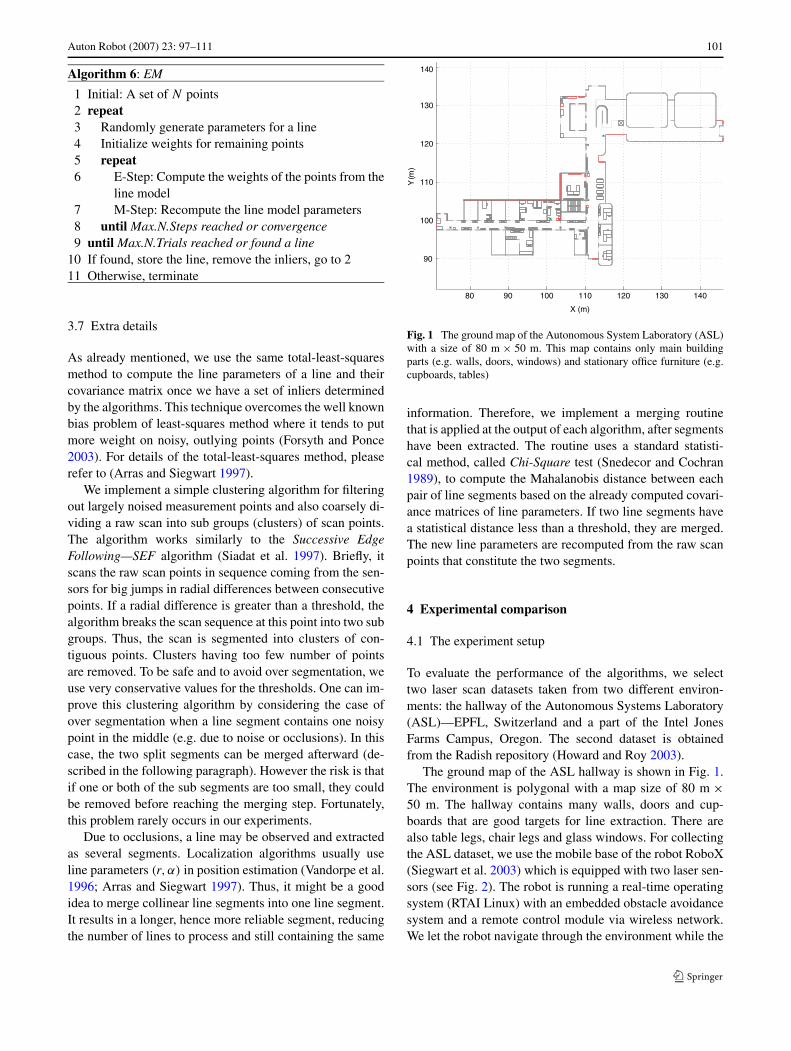
Fig. 1 The ground map of the Autonomous System Laboratory (ASL)with a size of 80 m × 50 m. This map contains only main buildingparts (e.g. walls, doors, windows) and stationary office furniture (e.g.cupboards, tables)

information. Therefore, we implement a merging routinethat is applied at the output of each algorithm, after segmentshave been extracted. The routine uses a standard statisti-cal method, called Chi-Square test (Snedecor and Cochran1989), to compute the Mahalanobis distance between eachpair of line segments based on the already computed covari-ance matrices of line parameters. If two line segments havea statistical distance less than a threshold, they are merged.The new line parameters are recomputed from the raw scanpoints that constitute the two segments.

4 Experimental comparison

4.1 The experiment setup

To evaluate the performance of the algorithms, we selecttwo laser scan datasets taken from two different environ-ments: the hallway of the Autonomous Systems Laboratory(ASL)—EPFL, Switzerland and a part of the Intel JonesFarms Campus, Oregon. The second dataset is obtainedfrom the Radish repository (Howard and Roy 2003).

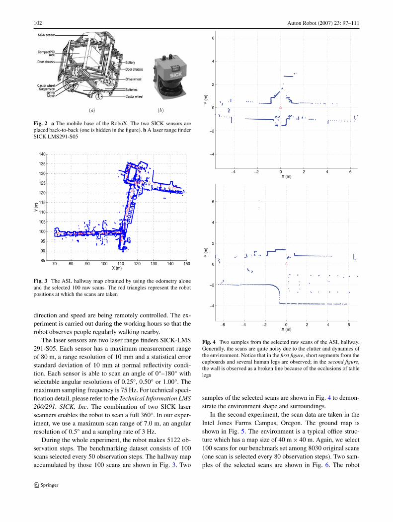
The ground map of the ASL hallway is shown in Fig. 1.The environment is polygonal with a map size of 80 m ×50 m. The hallway contains many walls, doors and cup-boards that are good targets for line extraction. There arealso table legs, chair legs and glass windows. For collectingthe ASL dataset, we use the mobile base of the robot RoboX(Siegwart et al. 2003) which is equipped with two laser sen-sors (see Fig. 2). The robot is running a real-time operatingsystem (RTAI Linux) with an embedded obstacle avoidancesystem and a remote control module via wireless network.We let the robot navigate through the environment while the

102 Auton Robot (2007) 23: 97–111

Fig. 2 a The mobile base of the RoboX. The two SICK sensors areplaced back-to-back (one is hidden in the figure). b A laser range finderSICK LMS291-S05

Fig. 3 The ASL hallway map obtained by using the odometry aloneand the selected 100 raw scans. The red triangles represent the robotpositions at which the scans are taken

direction and speed are being remotely controlled. The ex-periment is carried out during the working hours so that therobot observes people regularly walking nearby.

The laser sensors are two laser range finders SICK-LMS291-S05. Each sensor has a maximum measurement rangeof 80 m, a range resolution of 10 mm and a statistical errorstandard deviation of 10 mm at normal reflectivity condi-tion. Each sensor is able to scan an angle of 0°–180° withselectable angular resolutions of 0.25°, 0.50° or 1.00°. Themaximum sampling frequency is 75 Hz. For technical speci-fication detail, please refer to the Technical Information LMS200/291. SICK, Inc. The combination of two SICK laserscanners enables the robot to scan a full 360°. In our exper-iment, we use a maximum scan range of 7.0 m, an angularresolution of 0.5◦ and a sampling rate of 3 Hz.

During the whole experiment, the robot makes 5122 ob-servation steps. The benchmarking dataset consists of 100scans selected every 50 observation steps. The hallway mapaccumulated by those 100 scans are shown in Fig. 3. Two

Fig. 4 Two samples from the selected raw scans of the ASL hallway.Generally, the scans are quite noisy due to the clutter and dynamics ofthe environment. Notice that in the first figure, short segments from thecupboards and several human legs are observed; in the second figure,the wall is observed as a broken line because of the occlusions of tablelegs

samples of the selected scans are shown in Fig. 4 to demon-strate the environment shape and surroundings.

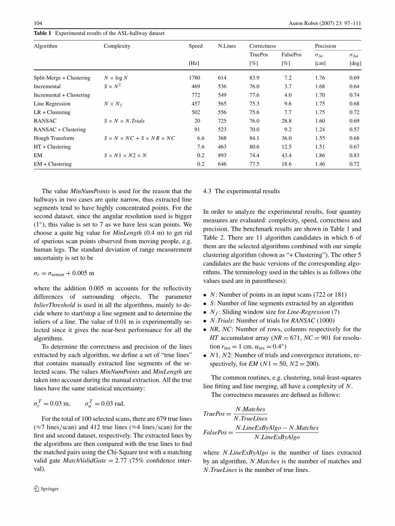
In the second experiment, the scan data are taken in theIntel Jones Farms Campus, Oregon. The ground map isshown in Fig. 5. The environment is a typical office struc-ture which has a map size of 40 m × 40 m. Again, we select100 scans for our benchmark set among 8030 original scans(one scan is selected every 80 observation steps). Two sam-ples of the selected scans are shown in Fig. 6. The robot

Auton Robot (2007) 23: 97–111 103

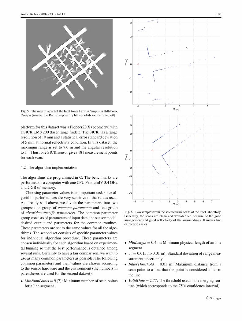
Fig. 5 The map of a part of the Intel Jones Farms Campus in Hillsboro,Oregon (source: the Radish repository http://radish.sourceforge.net/)

platform for this dataset was a Pioneer2DX (odometry) witha SICK LMS 200 (laser range finder). The SICK has a rangeresolution of 10 mm and a statistical error standard deviationof 5 mm at normal reflectivity condition. In this dataset, themaximum range is set to 7.0 m and the angular resolutionto 1◦. Thus, one SICK sensor gives 181 measurement pointsfor each scan.

4.2 The algorithm implementation

The algorithms are programmed in C. The benchmarks areperformed on a computer with one CPU PentiumIV-3.4 GHzand 2 GB of memory.

Choosing parameter values is an important task since al-gorithm performances are very sensitive to the values used.As already said above, we divide the parameters into twogroups: one group of common parameters and one groupof algorithm specific parameters. The common parametergroup consists of parameters of input data, the sensor model,desired output and parameters for the common routines.These parameters are set to the same values for all the algo-rithms. The second set consists of specific parameter valuesfor individual algorithm procedure. These parameters arechosen individually for each algorithm based on experimen-tal tunning so that the best performance is obtained amongseveral runs. Certainly to have a fair comparison, we want touse as many common parameters as possible. The followingcommon parameters and their values are chosen accordingto the sensor hardware and the environment (the numbers inparentheses are used for the second dataset):

• MinNumPoints = 9 (7): Minimum number of scan pointsfor a line segment.

Fig. 6 Two samples from the selected raw scans of the Intel laboratory.Generally, the scans are clean and well-defined because of the goodarrangement and good reflectivity of the surroundings. It makes lineextraction easier

• MinLength = 0.4 m: Minimum physical length of an linesegment.

• σr = 0.015 m (0.01 m): Standard deviation of range mea-surement uncertainty.

• InlierThreshold = 0.01 m: Maximum distance from ascan point to a line that the point is considered inlier tothe line.

• ValidGate = 2.77: The threshold used in the merging rou-tine (which corresponds to the 75% confidence interval).

104 Auton Robot (2007) 23: 97–111

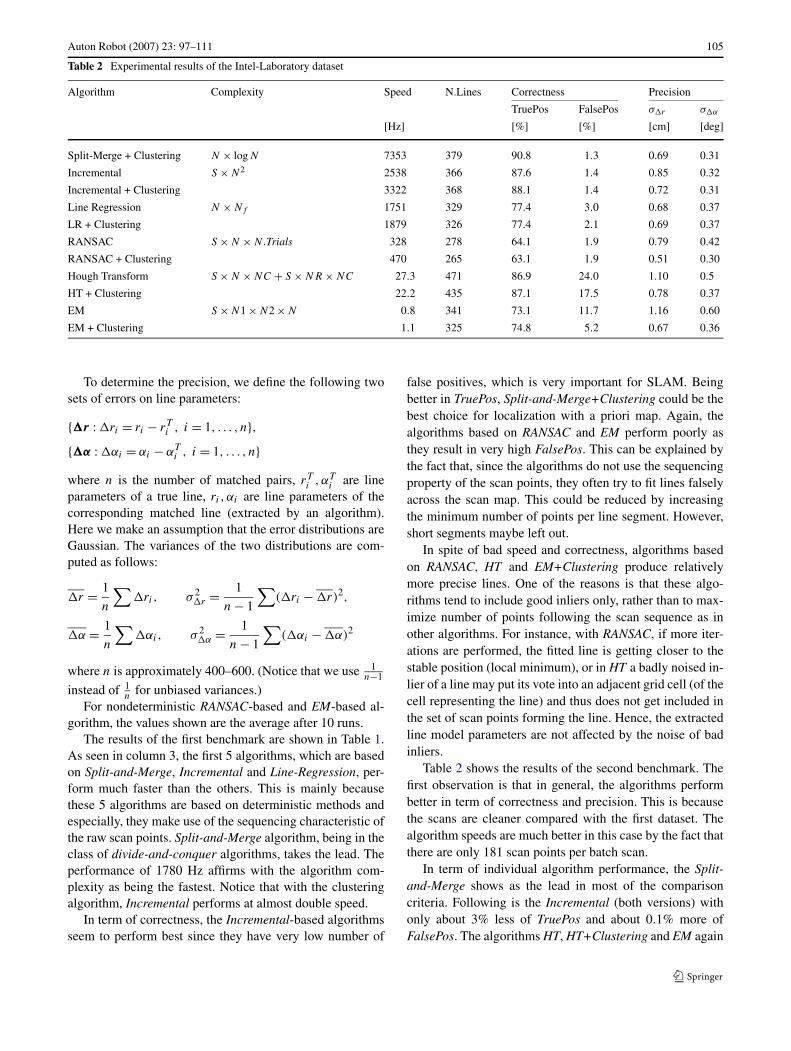
Table 1 Experimental results of the ASL-hallway dataset

Algorithm Complexity Speed N.Lines Correctness Precision

TruePos FalsePos σ�r σ�α

[Hz] [%] [%] [cm] [deg]

Split-Merge + Clustering N × logN 1780 614 83.9 7.2 1.76 0.69

Incremental S × N2 469 536 76.0 3.7 1.68 0.64

Incremental + Clustering 772 549 77.6 4.0 1.70 0.74

Line Regression N × Nf 457 565 75.3 9.6 1.75 0.68

LR + Clustering 502 556 75.6 7.7 1.75 0.72

RANSAC S × N × N.Trials 20 725 76.0 28.8 1.60 0.69

RANSAC + Clustering 91 523 70.0 9.2 1.24 0.57

Hough Transform S × N × NC + S × NR × NC 6.6 368 84.1 36.0 1.55 0.68

HT + Clustering 7.6 463 80.6 12.5 1.51 0.67

EM S × N1 × N2 × N 0.2 893 74.4 43.4 1.86 0.83

EM + Clustering 0.2 646 77.5 18.6 1.46 0.72

The value MinNumPoints is used for the reason that thehallways in two cases are quite narrow, thus extracted linesegments tend to have highly concentrated points. For thesecond dataset, since the angular resolution used is bigger(1◦), this value is set to 7 as we have less scan points. Wechoose a quite big value for MinLength (0.4 m) to get ridof spurious scan points observed from moving people, e.g.human legs. The standard deviation of range measurementuncertainty is set to be

σr = σsensor + 0.005 m

where the addition 0.005 m accounts for the reflectivitydifferences of surrounding objects. The parameterInlierThreshold is used in all the algorithms, mainly to de-cide where to start/stop a line segment and to determine theinliers of a line. The value of 0.01 m is experimentally se-lected since it gives the near-best performance for all thealgorithms.

To determine the correctness and precision of the linesextracted by each algorithm, we define a set of “true lines”that contains manually extracted line segments of the se-lected scans. The values MinNumPoints and MinLength aretaken into account during the manual extraction. All the truelines have the same statistical uncertainty:

σTr = 0.03 m, σ T

α = 0.03 rad.

For the total of 100 selected scans, there are 679 true lines(≈7 lines/scan) and 412 true lines (≈4 lines/scan) for thefirst and second dataset, respectively. The extracted lines bythe algorithms are then compared with the true lines to findthe matched pairs using the Chi-Square test with a matchingvalid gate MatchValidGate = 2.77 (75% confidence inter-val).

4.3 The experimental results

In order to analyze the experimental results, four quantitymeasures are evaluated: complexity, speed, correctness andprecision. The benchmark results are shown in Table 1 andTable 2. There are 11 algorithm candidates in which 6 ofthem are the selected algorithms combined with our simpleclustering algorithm (shown as “+ Clustering”). The other 5candidates are the basic versions of the corresponding algo-rithms. The terminology used in the tables is as follows (thevalues used are in parentheses):

• N : Number of points in an input scans (722 or 181)• S: Number of line segments extracted by an algorithm• Nf : Sliding window size for Line-Regression (7)• N.Trials: Number of trials for RANSAC (1000)• NR, NC: Number of rows, columns respectively for the

HT accumulator array (NR = 671, NC = 901 for resolu-tion rres = 1 cm, αres = 0.4◦)

• N1,N2: Number of trials and convergence iterations, re-spectively, for EM (N1 = 50, N2 = 200).

The common routines, e.g. clustering, total-least-squaresline fitting and line merging, all have a complexity of N .

The correctness measures are defined as follows:

TruePos = N.Matches

N.TrueLines

FalsePos = N.LineExByAlgo − N.Matches

N.LineExByAlgo

where N.LineExByAlgo is the number of lines extractedby an algorithm, N.Matches is the number of matches andN.TrueLines is the number of true lines.

Auton Robot (2007) 23: 97–111 105

Table 2 Experimental results of the Intel-Laboratory dataset

Algorithm Complexity Speed N.Lines Correctness Precision

TruePos FalsePos σ�r σ�α

[Hz] [%] [%] [cm] [deg]

Split-Merge + Clustering N × logN 7353 379 90.8 1.3 0.69 0.31

Incremental S × N2 2538 366 87.6 1.4 0.85 0.32

Incremental + Clustering 3322 368 88.1 1.4 0.72 0.31

Line Regression N × Nf 1751 329 77.4 3.0 0.68 0.37

LR + Clustering 1879 326 77.4 2.1 0.69 0.37

RANSAC S × N × N.Trials 328 278 64.1 1.9 0.79 0.42

RANSAC + Clustering 470 265 63.1 1.9 0.51 0.30

Hough Transform S × N × NC + S × NR × NC 27.3 471 86.9 24.0 1.10 0.5

HT + Clustering 22.2 435 87.1 17.5 0.78 0.37

EM S × N1 × N2 × N 0.8 341 73.1 11.7 1.16 0.60

EM + Clustering 1.1 325 74.8 5.2 0.67 0.36

To determine the precision, we define the following twosets of errors on line parameters:

{�r : �ri = ri − rTi , i = 1, . . . , n},

{�α : �αi = αi − αTi , i = 1, . . . , n}

where n is the number of matched pairs, rTi , αT

i are lineparameters of a true line, ri , αi are line parameters of thecorresponding matched line (extracted by an algorithm).Here we make an assumption that the error distributions areGaussian. The variances of the two distributions are com-puted as follows:

�r = 1

n

∑�ri, σ 2

�r = 1

n − 1

∑(�ri − �r)2,

�α = 1

n

∑�αi, σ 2

�α = 1

n − 1

∑(�αi − �α)2

where n is approximately 400–600. (Notice that we use 1n−1

instead of 1n

for unbiased variances.)For nondeterministic RANSAC-based and EM-based al-

gorithm, the values shown are the average after 10 runs.The results of the first benchmark are shown in Table 1.

As seen in column 3, the first 5 algorithms, which are basedon Split-and-Merge, Incremental and Line-Regression, per-form much faster than the others. This is mainly becausethese 5 algorithms are based on deterministic methods andespecially, they make use of the sequencing characteristic ofthe raw scan points. Split-and-Merge algorithm, being in theclass of divide-and-conquer algorithms, takes the lead. Theperformance of 1780 Hz affirms with the algorithm com-plexity as being the fastest. Notice that with the clusteringalgorithm, Incremental performs at almost double speed.

In term of correctness, the Incremental-based algorithmsseem to perform best since they have very low number of

false positives, which is very important for SLAM. Beingbetter in TruePos, Split-and-Merge+Clustering could be thebest choice for localization with a priori map. Again, thealgorithms based on RANSAC and EM perform poorly asthey result in very high FalsePos. This can be explained bythe fact that, since the algorithms do not use the sequencingproperty of the scan points, they often try to fit lines falselyacross the scan map. This could be reduced by increasingthe minimum number of points per line segment. However,short segments maybe left out.

In spite of bad speed and correctness, algorithms basedon RANSAC, HT and EM+Clustering produce relativelymore precise lines. One of the reasons is that these algo-rithms tend to include good inliers only, rather than to max-imize number of points following the scan sequence as inother algorithms. For instance, with RANSAC, if more iter-ations are performed, the fitted line is getting closer to thestable position (local minimum), or in HT a badly noised in-lier of a line may put its vote into an adjacent grid cell (of thecell representing the line) and thus does not get included inthe set of scan points forming the line. Hence, the extractedline model parameters are not affected by the noise of badinliers.

Table 2 shows the results of the second benchmark. Thefirst observation is that in general, the algorithms performbetter in term of correctness and precision. This is becausethe scans are cleaner compared with the first dataset. Thealgorithm speeds are much better in this case by the fact thatthere are only 181 scan points per batch scan.

In term of individual algorithm performance, the Split-and-Merge shows as the lead in most of the comparisoncriteria. Following is the Incremental (both versions) withonly about 3% less of TruePos and about 0.1% more ofFalsePos. The algorithms HT, HT+Clustering and EM again

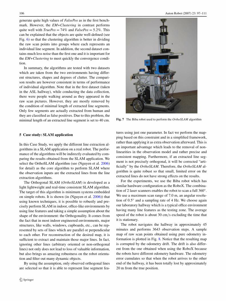
106 Auton Robot (2007) 23: 97–111

generate quite high values of FalsePos as in the first bench-mark. However, the EM+Clustering in contrast performsquite well with TruePos = 74% and FalsePos = 5.2%. Thiscan be explained that the objects are quite well-defined (seeFig. 6) so that the clustering algorithm is better in dividingthe raw scan points into groups where each represents anindividual line segment. In addition, the second dataset con-tains much less noise than the first one and it is important forthe EM+Clustering to meet quickly the convergence condi-tion.

In summary, the algorithms are tested with two datasetswhich are taken from the two environments having differ-ent structures, shapes and degrees of clutter. The compari-son results are however consistent in terms of performanceof individual algorithm. Note that in the first dataset (takenin the ASL hallway), while conducting the data collection,there were people walking around as they appeared in theraw scan pictures. However, they are mostly removed bythe condition of minimal length of extracted line segments.Only few segments are actually extracted from human andthey are classified as false positives. Due to this problem, theminimal length of an extracted line segment is set to 40 cm.

5 Case study: SLAM application

In this Case Study, we apply the different line extraction al-gorithms in a SLAM application on a real robot. The perfor-mance of the algorithms will be indirectly evaluated by com-paring the results obtained from the SLAM application. Weselect the OrthoSLAM algorithm (see (Nguyen et al. 2006)for detail) as the core algorithm to perform SLAM wherethe observation inputs are the extracted lines from the lineextraction algorithms.

The Orthogonal SLAM (OrthoSLAM) is developed as alight lightweight and real-time consistent SLAM algorithm.The target of this algorithm is minimum systems embeddedon simple robots. It is shown (in (Nguyen et al. 2006)) thatusing known techniques, it is possible to robustly and pre-cisely perform SLAM in indoor, office-like environments byusing line features and taking a simple assumption about theshape of the environment: the Orthogonality. It comes fromthe fact that in most indoor engineered environments, majorstructures, like walls, windows, cupboards, etc., can be rep-resented by sets of lines which are parallel or perpendicularto each other. For reconstruction of the desired map, it issufficient to extract and maintain those major lines. In fact,ignoring other lines (arbitrary oriented or non-orthogonallines) not only does not lead to loss of valuable information,but also brings us amazing robustness on the robot orienta-tion and filter out many dynamic objects.

By using the assumption, only observed orthogonal linesare selected so that it is able to represent line segment fea-

Fig. 7 The Biba robot used to perform the OrthoSLAM algorithm

tures using just one parameter. In fact we perform the map-ping based on this constraint and in a simplified framework,rather than applying it as extra observation afterward. This isan important advantage which leads to the removal of non-linearities in the observation model and rather precise andconsistent mapping. Furthermore, if an extracted line seg-ment is not precisely orthogonal, it will be corrected “arti-ficially” by the OrthoSLAM. Therefore, the OrthoSLAM al-gorithm is quite robust so that small, limited error on theextracted lines do not have strong effects on the results.

For the experiments, we use the Biba robot which hassimilar hardware configuration as the RoboX. The combina-tion of 2 laser scanners enables the robot to scan a full 360◦.We use a maximum scan range of 7.0 m, an angular resolu-tion of 0.5◦ and a sampling rate of 4 Hz. We choose againour laboratory hallway which is a typical office environmenthaving many line features as the testing zone. The averagespeed of the robot is about 30 cm/s excluding the time thatit is stationary.

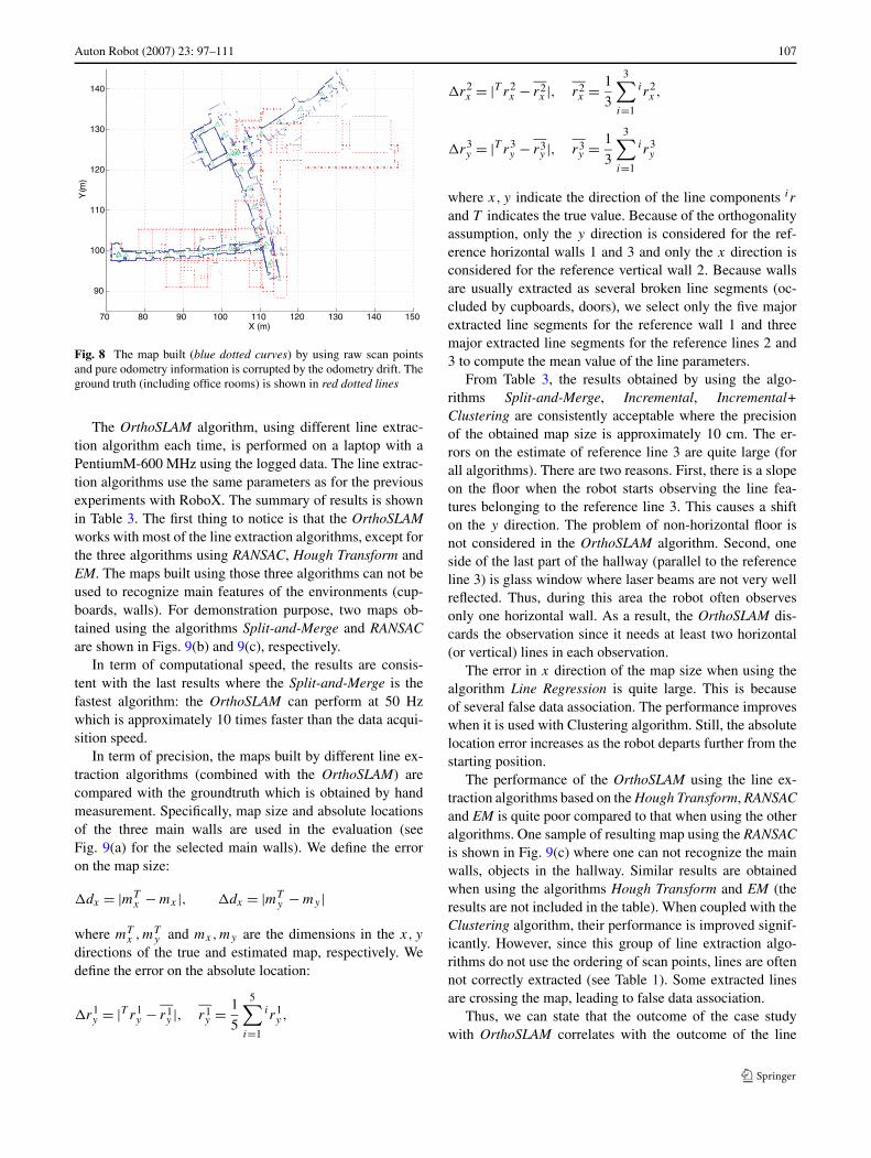
The robot navigates the hallway in approximately 45minutes and performs 3643 observation steps. A samplemap of raw scan points obtained using pure odometry in-formation is plotted in Fig. 8. Notice that the resulting mapis corrupted by the odometry drift. The drift is also differ-ent from the one obtained when using the RoboX becausethe robots have different odometry hardware. The odometryerror cumulates so that when the robot arrives to the otherend of the hallway, it has been totally lost by approximately20 m from the true position.

Auton Robot (2007) 23: 97–111 107

Fig. 8 The map built (blue dotted curves) by using raw scan pointsand pure odometry information is corrupted by the odometry drift. Theground truth (including office rooms) is shown in red dotted lines

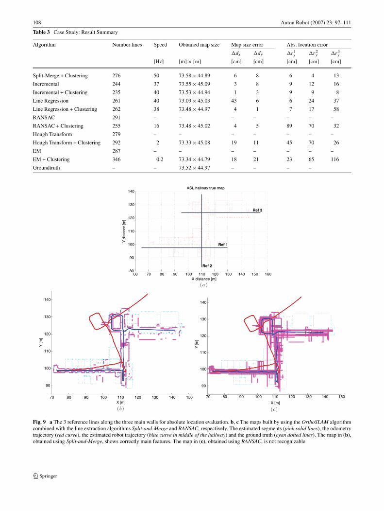
The OrthoSLAM algorithm, using different line extrac-tion algorithm each time, is performed on a laptop with aPentiumM-600 MHz using the logged data. The line extrac-tion algorithms use the same parameters as for the previousexperiments with RoboX. The summary of results is shownin Table 3. The first thing to notice is that the OrthoSLAMworks with most of the line extraction algorithms, except forthe three algorithms using RANSAC, Hough Transform andEM. The maps built using those three algorithms can not beused to recognize main features of the environments (cup-boards, walls). For demonstration purpose, two maps ob-tained using the algorithms Split-and-Merge and RANSACare shown in Figs. 9(b) and 9(c), respectively.

In term of computational speed, the results are consis-tent with the last results where the Split-and-Merge is thefastest algorithm: the OrthoSLAM can perform at 50 Hzwhich is approximately 10 times faster than the data acqui-sition speed.

In term of precision, the maps built by different line ex-traction algorithms (combined with the OrthoSLAM) arecompared with the groundtruth which is obtained by handmeasurement. Specifically, map size and absolute locationsof the three main walls are used in the evaluation (seeFig. 9(a) for the selected main walls). We define the erroron the map size:

�dx = |mTx − mx |, �dx = |mT

y − my |

where mTx ,mT

y and mx,my are the dimensions in the x, y

directions of the true and estimated map, respectively. Wedefine the error on the absolute location:

�r1y = |T r1

y − r1y |, r1

y = 1

5

5∑i=1

i r1y ,

�r2x = |T r2

x − r2x |, r2

x = 1

3

3∑i=1

i r2x ,

�r3y = |T r3

y − r3y |, r3

y = 1

3

3∑i=1

i r3y

where x, y indicate the direction of the line components i r

and T indicates the true value. Because of the orthogonalityassumption, only the y direction is considered for the ref-erence horizontal walls 1 and 3 and only the x direction isconsidered for the reference vertical wall 2. Because wallsare usually extracted as several broken line segments (oc-cluded by cupboards, doors), we select only the five majorextracted line segments for the reference wall 1 and threemajor extracted line segments for the reference lines 2 and3 to compute the mean value of the line parameters.

From Table 3, the results obtained by using the algo-rithms Split-and-Merge, Incremental, Incremental+Clustering are consistently acceptable where the precisionof the obtained map size is approximately 10 cm. The er-rors on the estimate of reference line 3 are quite large (forall algorithms). There are two reasons. First, there is a slopeon the floor when the robot starts observing the line fea-tures belonging to the reference line 3. This causes a shifton the y direction. The problem of non-horizontal floor isnot considered in the OrthoSLAM algorithm. Second, oneside of the last part of the hallway (parallel to the referenceline 3) is glass window where laser beams are not very wellreflected. Thus, during this area the robot often observesonly one horizontal wall. As a result, the OrthoSLAM dis-cards the observation since it needs at least two horizontal(or vertical) lines in each observation.

The error in x direction of the map size when using thealgorithm Line Regression is quite large. This is becauseof several false data association. The performance improveswhen it is used with Clustering algorithm. Still, the absolutelocation error increases as the robot departs further from thestarting position.

The performance of the OrthoSLAM using the line ex-traction algorithms based on the Hough Transform, RANSACand EM is quite poor compared to that when using the otheralgorithms. One sample of resulting map using the RANSACis shown in Fig. 9(c) where one can not recognize the mainwalls, objects in the hallway. Similar results are obtainedwhen using the algorithms Hough Transform and EM (theresults are not included in the table). When coupled with theClustering algorithm, their performance is improved signif-icantly. However, since this group of line extraction algo-rithms do not use the ordering of scan points, lines are oftennot correctly extracted (see Table 1). Some extracted linesare crossing the map, leading to false data association.

Thus, we can state that the outcome of the case studywith OrthoSLAM correlates with the outcome of the line

108 Auton Robot (2007) 23: 97–111

Table 3 Case Study: Result Summary

Algorithm Number lines Speed Obtained map size Map size error Abs. location error

�dx �dy �r1y �r2

y �r3y

[Hz] [m] × [m] [cm] [cm] [cm] [cm] [cm]

Split-Merge + Clustering 276 50 73.58 × 44.89 6 8 6 4 13

Incremental 244 37 73.55 × 45.09 3 8 9 12 16

Incremental + Clustering 235 40 73.53 × 44.94 1 3 9 9 8

Line Regression 261 40 73.09 × 45.03 43 6 6 24 37

Line Regression + Clustering 262 38 73.48 × 44.97 4 1 7 17 58

RANSAC 291 – – – – – – –

RANSAC + Clustering 255 16 73.48 × 45.02 4 5 89 70 32

Hough Transform 279 – – – – – – –

Hough Transform + Clustering 292 2 73.33 × 45.08 19 11 45 70 26

EM 287 – – – – – – –

EM + Clustering 346 0.2 73.34 × 44.79 18 21 23 65 116

Groundtruth – – 73.52 × 44.97 – – – –

Fig. 9 a The 3 reference lines along the three main walls for absolute location evaluation. b, c The maps built by using the OrthoSLAM algorithmcombined with the line extraction algorithms Split-and-Merge and RANSAC, respectively. The estimated segments (pink solid lines), the odometrytrajectory (red curve), the estimated robot trajectory (blue curve in middle of the hallway) and the ground truth (cyan dotted lines). The map in (b),obtained using Split-and-Merge, shows correctly main features. The map in (c), obtained using RANSAC, is not recognizable

Auton Robot (2007) 23: 97–111 109

extraction experiments. Clustering as well as correctnesshave a direct impact on the map estimation. Because Or-thoSLAM makes use of the orthogonality assumption, cor-rectness is more important than precision. The line extrac-tion algorithms RANSAC, Hough Transform and EM are out-performed by the other algorithms even though their preci-sion is higher.

6 Conclusions

This paper has presented an experimental evaluation of thesix line extraction algorithms using 2D laser scanner whichare commonly used for feature extraction in mobile robot-ics and computer vision. The basic versions of the algo-rithms are implemented and tested with two datasets takenfrom two office environments which have different struc-tures, shapes and degrees of clutter. Line segments extractedby the algorithms are compared with the manually extractedlines using standard statistical methods. Several comparisoncriteria are proposed and used to discuss in details their ad-vantages and drawbacks. Additionally, the line extractionalgorithms are tested in the OrthoSLAM application andthe results obtained individually are compared. We believethis is important, particularly in mobile robotics, that tech-niques or algorithms should be tested and verified their per-formance in real life application before we can make the fi-nal choice. The comparison result with the OrthoSLAM hasbeen shown to agree with the findings in the first part, thusagain verify the conclusions.

Overall, the experimental results show that the two al-gorithms Split-and-Merge and Incremental have best perfor-mance because of their superior speed and correctness. Forreal-time applications, Split-and-Merge is clearly the bestchoice by its superior speed. It is also the first choice forlocalization problems with a priori map, where FalsePos isnot very important. However, a right choice highly dependson the applications and implementation details as the casestudy showed, where correctness is favored over precision.

The first released version of the implementation is ac-cessible to public at http://www.asl.ethz.ch/people/tnguyen/.The ASL dataset can also be downloaded from the same lo-cation for comparison purposes. Interested user can send in-quiries to viet.nguyen@mavt.ethz.ch.

Acknowledgements This work has been supported by the SwissNational Science Foundation No. 200021-101886 and the EU projectCogniron FP6-IST-002020. We would like to thank Frédéric Pont forthe support in carrying out the experiments. The Intel Oregon datasetwas obtained from the Robotics Data Set Repository (Radish). Thanksgo to Maxim Batalin for providing the data.

References

Adams, M. D., & Kerstens, A. (1998). Tracking naturally occurringindoor features in 2D and 3D with lidar range/amplitude data. In-ternational Journal of Robotics Research, 17(9), 907–923.

Alempijevic, A. (2004). High-speed feature extraction in sensor coor-dinates for laser rangefinders. In Proceedings of the Australasianconference on robotics and automation.

Arras, K. O., & Siegwart, R. (1997). Feature extraction and scene in-terpretation for map-based navigation and map building. In Pro-ceedings of the symposium on intelligent systems and advancedmanufacturing.

Borges, G. A., & Aldon, M.-J. (2004). Line extraction in 2D rangeimages for mobile robotics. Journal of Intelligent and Robotic Sys-tems, 40, 267–297.

Brunskill, E., & Roy, N. (2005). SLAM using incremental probabilisticPCA and dimensionality reduction. In Proceedings of the IEEEinternational conference on robotics and automation.

Castellanos, J., & Tardós, J. (1996). Laser-based segmentation andlocalization for a mobile robot. In Robotics and manufacturing:recent trends in research and applications (Vol. 6). New York:ASME.

Cox, I. J. (1991). Blanche: an experiment in guidance and navigationof an autonomous robot vehicle. IEEE Transactions on Roboticsand Automation, 7(2), 193–204.

Crowley, J. L. (1985). Navigation for an Intelligent mobile robot. IEEEJournal of Robotics and Automation, 1(1), 31–41.

Diosi, A., & Kleeman, L. (2003a). Uncertainty of line segments ex-tracted from static SICK PLS laser scans. In Proceedings of theAustralasian conference on robotics and automation.

Diosi, A., & Kleeman, L. (2003b). Uncertainty of line segments ex-tracted from static SICK PLS laser scans. Department of Electri-cal and Computer Systems Engineering, Monash University, Tech.Rep. MECSE-26-2003.

Duda, R. O., & Hart, P. E. (1973). Pattern classification and sceneanalysis. New York: Wiley.

Einsele, T. (1997). Real-time self-localization in unknown indoor en-vironments using a panorama laser range finder. In Proceedingsof the IEEE/RSJ international conference on intelligent robots andsystems (pp. 697–702).

Fischler, M., & Bolles, R. (1981). Random sample consensus: A para-digm for model fitting with application to image analysis and auto-mated cartography. Communications of the ACM, 24(6), 381–395.

Forsberg, J., Larsson, U., & Wernersson, A. (1995). Mobile robot nav-igation using the range-weighted hough transform. IEEE Roboticsand Automation Magazine, 2(1), 18–26.

Forsyth, D. A., & Ponce, J. (2003). Computer vision: a modern ap-proach. New York: Prentice Hall.

Gutmann, J.-S., & Schlegel, C. (1996). AMOS: comparison of scanmatching approaches for self-localization in indoor environments.In First European workshop on advanced mobile robots (Eurobot).

Gutmann, J.-S., Burgard, W., Fox, D., & Konolige, K. (1998). An ex-perimental comparison of localization methods. In Proceedings ofthe IEEE/RSJ intenational conference on intelligent robots andsystems, IROS.

Howard, A., & Roy, N. (2003). The robotics data set repository(radish). Available: http://radish.sourceforge.net/.

Iocchi, L., & Nardi, D. (2002). Hough localization for mobile robots inpolygonal environments. Robotics and Autonomous Systems, 40,43–58.

Iyengar, S., & Elfes, A. (1991). Autonomous mobile robots (Vols. 1, 2).Los Alamitos: IEEE Computer Society.

Jensfelt, P., & Christensen, H. (1998). Laser based position acquisitionand tracking in an indoor environment. In Proceedings of the IEEEinternational symposium on robotics and automation (vol. 1).

110 Auton Robot (2007) 23: 97–111

Leonard, J., Cox, I. J., & Durrant-Whyte, H. (1992). Dynamic mapbuilding for an autonomous mobile robot. International Journal ofRobotics Research, 11(4), 286–298.

Liu, Y., Emery, R., Chakrabarti, D., Burgard, W., & Thrun, S. (2001).Using EM to learn 3D models of indoor environments with mobilerobots. In Proceedings of the IEEE international conference onmachine learning (ICML).

Lu, F., & Milios, E. (1994). Robot pose estimation in unknown en-vironments by matching 2D range scans. In Proceedings of theIEEE computer society conference on computer vision and patternrecognition (pp. 935–938).

Nguyen, V., Martinelli, A., Tomatis, N., & Siegwart, R. (2005). A com-parison of line extraction algorithms using 2D laser rangefinder forindoor mobile robotics. In Proceedings of the IEEE/RSJ intena-tional conference on intelligent robots and systems, IROS, Edmon-ton, Canada.

Nguyen, V., Harati, A., Tomatis, N., Martinelli, A., & Siegwart,R. (2006). OrthoSLAM: a step toward lightweight indoor au-tonomous navigation. In Proceedings of the IEEE/RSJ intena-tional conference on intelligent robots and systems, IROS, Beijing,China.

Pavlidis, T., & Horowitz, S. L. (1974). Segmentation of plane curves.IEEE Transactions on Computers, C-23(8), 860–870.

Pears, N. (2000). Feature extraction and tracking for scanning rangesensors. Robotics and Autonomous Systems, 33, 43–58.

Pfister, S. T., Roumeliotis, S. I., & Burdick, J. W. (2003). Weightedline fitting algorithms for mobile robot map building and efficientdata representation. In Proceedings of the IEEE international con-ference on robotics and automation, ICRA (pp. 1304–1311).

Sack, D., & Burgard, W. (2004). A comparison of methods for lineextraction from range data. In Proceedings of the 5th IFAC sympo-sium on intelligent autonomous vehicles.

Schröter, D., Beetz, M., & Gutmann, J.-S. (2002). RG mapping: learn-ing compact and structured 2D line maps of indoor environments.In Proceedings of 11th IEEE international workshop on robot andhuman interactive communication (ROMAN).

Siadat, A., Kaske, A., Klausmann, S., Dufaut, M., & Husson, R.(1997). An optimized segmentation method for a 2D laser-scannerapplied to mobile robot navigation. In Proceedings of the 3rd IFACsymposium on intelligent components and instruments for controlapplications.

Siegwart, R., Arras, K. O., Bouabdallah, S., Burnier, D., Froidevaux,G., Greppin, X., Jensen, B., Lorotte, A., Mayor, L., Meisser, M.,Philippsen, R., Piguet, R., Ramel, G., Terrien, G., & Tomatis, N.(2003). Robox at Expo.02: a large scale installation of personalrobots. Special issue on Socially Interactive Robots, Robotics andAutonomous Systems, 42, 203–222.

Snedecor, G. W., & Cochran, W. G. (1989). Statistical methods (8thed.). Ames: Iowa State University Press.

Taylor, R., & Probert, P. (1996). Range finding and feature extractionby segmentation of images for mobile robot navigation. In Pro-ceedings of the IEEE international conference on robotics and au-tomation, ICRA.

Tomatis, N., Nourbakhsh, I., & Siegwart, R. (2003). Hybrid simulta-neous localization and map building: a natural integration of topo-logical and metric. Robotics and Autonomous Systems, 44, 3–14.

Vandorpe, J., Brussel, H. V., & Xu, H. (1996). Exact dynamic mapbuilding for a mobile robot using geometrical primitives producedby a 2D range finder. In Proceedings of the IEEE internationalconference on robotics and automation, ICRA (pp. 901–908).

Xu, L., Oja, E., & Kultanen, P. (1990). A new curve detection method:randomized hough transform (RHT). Pattern Recognition Letters,11(5), 331–338.

Zhang, L., & Ghosh, B. K. (2000). Line segment based map buildingand localization using 2D laser rangefinder. In Proceedings of theIEEE international conference on robotics and automation, ICRA.

Viet Nguyen is a Ph.D. student at the SwissFederal Institute of Technology Lausanne(EPFL). He received his Bachelor in SoftwareEngineering from the Australian National Uni-versity, Australia in 1999. He worked as a re-search assistant in the Laboratory of ArtificialIntelligence at EPFL in 2001. In 2003, he joinedthe Autonomous Systems Laboratory wherestarted his Ph.D. study under the supervisionof Professor Siegwart. Since July 2006, he has

been working at the Autonomous Systems Laboratory at the SwissFederal Institute of Technology Zurich (ETHZ). His research coveredmobile robot navigation, SLAM, feature extraction, data association,constraint satisfaction and optimization.

Stefan Gächter received the Master’s degree inelectrical engineering from the École Polytech-nique Fédérale de Lausanne (EPFL), Switzer-land, in 2001. After his master’s studies, hespent three years as a research engineer in thefield of active magnetic bearings at Koyo SeikoCo. Ltd, Japan. He joined the Autonomous Sys-tems Lab (ASL), École Polytechnique Fédéralede Lausanne (EPFL), Switzerland, in 2004,where he commenced work towards a Ph.D. de-

gree. Since July 2006, the Autonomous Systems Lab has been based atthe Eidgenössische Technische Hochschule Zürich (ETHZ), Switzer-land. His research interest is in computer vision for mobile roboticswith emphasis on probabilistic algorithms for object classification ap-plied to range images.

Agostino Martinelli (1971) received the M.Sc.in theoretical Physics in 1994 from the Univer-sity of Rome “Tor Vergat” and the PhD in As-trophysics in 1999 from the University of Rome“La Sapienza”. During his PhD he spent oneyear at the University of Wales in Cardiff andone year in the School of Trieste (SISSA). Hisresearch was focused on the chemical and dy-namical evolution in the elliptical galaxies, inthe quasars and in the intergalactic medium. He

also introduced models based on the General Relativity to explain theanisotropies on the Cosmic Background Radiation. After his PhD, hisinterests moved on the problem of autonomous navigation. He spenttwo years in the University of Rome “Tor Vergata” and, in 2002, hemoved to the Autonomous Systems Lab, EPFL, in Lausanne as seniorresearcher, where he was leading several projects on multi sensor fu-sion for robot localization (with particular attention to the odometrysensors), simultaneous localization and odometry error learning, andsimultaneous localization and map building. Since September 2006 heis First Researcher (CR1) at the INRIA Rhone Alpes in Grenoble. Hehas authored/co-authored more than 30 journals and conference papers.

Nicola Tomatis (1973) received his M.Sc. incomputer science in 1998 from the Swiss Fed-eral Institute of Technology (ETH) Zurich. Af-ter working as assistant for the Institute of Ro-botics, ETH, he moved to the Swiss Federal In-stitute of Technology (EPFL) Lausanne, wherehe received his Ph.D. at the end of 2001. His re-search covered metric and topological (hybrid)mobile robot navigation, computer vision andsensor data fusion. From 2001 to 2005 he had a

Auton Robot (2007) 23: 97–111 111

part time position as senior researcher with the Autonomous SystemsLab, EPFL (now ETH), where he was leading several projects and con-tinuing his research in navigation, man–machine interaction and robotsafety and reliability. He has authored/co-authored more than 35 jour-nals and conference papers. During 2001 he joined BlueBotics SA,a SME involved in mobile robotics. Since year 2003 he is CEO of thecompany. http://asl.epfl.ch, http://www.bluebotics.com

Roland Siegwart is full professor for au-tonomous systems at ETH Zurich since July2006. He has a Diploma in Mechanical Engi-neering (1983) and PhD in Mechatronics (1989)from ETH Zurich. In 1989/90 he spent one yearas postdoctoral fellow at Stanford University.After that he worked part time as R&D di-rector at MECOS Traxler AG and as lecturerand deputy head at the Institute of Robotics,ETH Zürich. In 1996 he was appointed as as-

sociate and later full professor for autonomous microsystems and ro-bots at the Ecole Polytechnique Fédérale de Lausanne (EPFL). Dur-ing his period at EPFL he was Deputy Head of the National Compe-tence Center for Research (NCCR) on Multimodal Information Man-agement (IM2), co-initiator and founding Chairman of Space Cen-ter EPFL and Vice Dean of the School of Engineering. In 2005 hehold a visiting position at NASA Ames and Stanford University.Roland Siegwart is member of the Swiss Academy of EngineeringSciences and board member of the European Network of Robot-ics (EURON). He served as Vice President for Technical Activities(2004/05) and is currently Distinguished Lecturer (2006/07) and Ad-Com Member (2007–2009) of the IEEE Robotics and Automation So-ciety. He is member of the “Bewilligungsausschuss Exzellenzinitia-tive” of the “Deutsche Forschungsgemeinschaft (DFG)”. He is coor-dinator of two European projects and co-founder of several spin-offcompanies.