A case study investigating the impacts of coagulants on taste and odour reduction in drinking

water

A thesis submitted in fulfilment of the requirements for the degree of Master of Engineering

Tara Jane Callingham

Bachelor of Engineering (Honours) University of New South Wales

School of Engineering

College of Science, Engineering and Health

RMIT University

August 2017

2

Declaration

I certify that except where due acknowledgement has been made, the work is that of the author

alone; the work has not been submitted previously, in whole or in part, to qualify for any other

academic award; the content of the thesis/project is the result of work which has been carried

out since the official commencement date of the approved research program; any editorial

work, paid or unpaid, carried out by a third party is acknowledged; and, ethics procedures and

guidelines have been followed.

Tara Jane Callingham

30th August 2017

3

Acknowledgements

I have so many people to thank, I am not even entirely sure where to start! Working full time

and undertaking a research project is by far one of the hardest things I think I have ever done

and the support of people around me has kept me going throughout the process!

I think obviously I need to start with my supervisors; Felicity Roddick, Linhua Fan and Daniel

Ooi. With particular mention to Felicity, who I am sure has found me a struggle at times. Her

incredible patience when reading some of the drivel given to her in the early stages of this

process is much appreciated!

Secondly, I would never have been able to complete this project without the support of GVW.

In particular I would like to mention Alan Tyson, for his enthusiasm at getting this process

underway, Mark Putman, for his support throughout the project and Steven Nash for his

unwavering belief that I would actually finish this and his desire to see the findings

implemented. I obviously could never have got as far as I did without the help of the operators

and their complete honesty when discussing the process and what they do. Their support for

me throughout this process is heart-warming and I am sure that they were supportive despite

of the fact they got the benefit of using my jar tests! My workgroup, Chris, Brenda, Steve and

Sandy have been amazing in the last few months, in particular Steve has been amazing helping

me out with my “not so stupid questions”.

I would also like to thank Water Research Australia for their support through this and allowing

me to be their first industry masters student! In particular thanks to Carolyn Bellamy for

organising the process and getting me underway!

Obviously, my family get a mention, and their consistent pushing of the Family Motto “head

down, bum up and get it done”. Especially my mother for her proof reading and statistical

help.

Finally, thank you so very much to Samuel Daniel. Your patience, love and support,

particularly in the last 8 months, is so very much appreciated and I am incredibly grateful to

you and to have you in my life. I don’t think I would have made it through this mentally intact

without you, so thank you for making everything better (and keeping the house clean!)

4

Summary

Goulburn Valley Water (GVW) is a regional water business that provides water and waste

water services to 54 towns across 20,000 km2 in Northern Victoria. Taste and odour issues

across the region resulted in this case study to investigate improvements through optimisation

of existing treatment processes.

Historically, Euroa has had problems with taste and odour although, there are limited numbers

of formal complaints recorded in widespread locations across the town. A Taste and Odour

Panel determined the key odours in the reticulation system were earthy /musty and chlorine,

with the panel unable to determine any specific tastes. The free chlorine residual at the point

of entry to the reticulation system, which is consistently above the Australian Drinking Water

Guidelines aesthetic limit for chlorine, was the cause of the chlorine odours detected.

Odours detected by the panel in reticulated water samples were correlated against water

quality parameters. These showed there were some relationships between the identified odours

and specific ultraviolet absorbance (SUVA). In addition, the level of free chlorine residual at

the point of disinfection and at the outlet of the clear water storage was related to the number

of chlorine and earthy /musty odours detected. As the odours appeared to be related to the

levels of natural organic matter (NOM) within the source water, its removal through

optimisation of the existing process and the use of alternative chemicals was investigated.

The existing water treatment plant (WTP) operation was reviewed for NOM removal and the

coagulant dose optimised. Ferric sulphate and aluminium chlorohydrate (ACH) were trialled

as alternative coagulants as these traditionally have a higher affinity for dissolved organic

carbon (DOC) removal than aluminium sulphate currently in use.

The SUVA values seen at Euroa WTP indicate that the removal pathway for organic matter is

predominantly through coagulation. Jar tests were completed to optimise the existing

coagulant dose rate as well as the investigation into the alternative coagulants.

The following key points were determined from the jar tests:

Ferric sulphate results were as expected showing a greater average DOC removal than

the other samples (72 %);

ACH provided lower than expected DOC removal rates (59 %);

Aluminium sulphate gave consistent average DOC removal results for both the jar test

and the WTP (55 % and 57 %, respectively).

Odour testing was completed following jar tests using the original taste and odour panel.

The Chi squared statistic was used to calculate the expected values based on the observed

odours. The following key points were determined from the odour testing results:

5

The number of earthy /musty odours detected decreased against the expected value

when using ACH and the number of no odour detections were greater than the

expected value;

The number of other odour detects were greater than the expected value when using

ferric sulphate, however there were fewer earthy /musty odours detected than the

expected value;

The number of earthy /musty odours were greater than the expected values from the

WTP samples;

The number of earthy /musty odours were equal to the expected value for the

aluminum sulphate sample.

Optimisation of the aluminium sulphate coagulation for organics removal did not appear to

reduce the number of earthy /musty odours detected. The use of ferric sulphate or ACH would

improve the odour of the final water at Euroa WTP.

A triple bottom line (TBL) assessment was completed to assess the economic, social and

environmental impacts of each of the coagulants compared with the current practice.

The cost of treatment was determined based on jar test results, the cost of sludge disposal and

the impact on the GVW infrastructure program was reviewed. The key findings associated

with the economic assessment are as follows;

The use of ACH would provide a saving of $6,345 based on chemicals and $2,581

based on sludge disposal costs, with the potential to defer $1.1 million in capital

expenditure;

The use of ferric sulphate would provide an increase of $9,796 based on chemicals

and $526 based on sludge disposal costs, with no impact on the infrastructure

program;

The optimisation of aluminium sulphate coagulation would provide a saving of $3,380

based on chemicals and $90 based on sludge disposal costs, with no impact on the

infrastructure program.

The environmental impacts of each chemical were assessed based on their potential offsite

impacts. The potential for sending waste sludge to landfill was assessed as well as the potential

carbon emissions associated with the delivery of chemical coagulants. The key findings from

the environmental assessment are as follows:

The use of ferric sulphate produced the most sludge therefore creating a greater

volume of waste to be sent to landfill;

The use of ACH created minimal sludge and therefore has a lower landfill potential;

6

Optimisation of the aluminium sulphate coagulation created slightly less sludge than

the WTP, therefore had a slightly lower landfill potential;

Ferric sulphate and ACH dose rates were lower than the aluminum sulphate and WTP

dose rates therefore requiring fewer deliveries (ferric sulphate 5, ACH 2 deliveries

respectively) across the year;

The aluminum sulphate and current WTP chemical delivery requirements were

considered to be the same (7 deliveries each based on 10,000 L deliveries);

For pH correction there was no difference in the requirements for ferric sulphate and

the current operation (2 deliveries for each annually based on 10,000 L delivery);

The ACH requires no pre pH correction therefore the post pH dosing only is required.

This equated to a single chemical delivery per year.

The social impacts on the community and GVW staff were assessed based on the changes in

odours. Since some residents within the Euroa connected to town water still maintain a

rainwater tank for drinking purposes based on the taste and odour of the drinking water. It is

assumed that with improved odour in time they would begin to use town water for drinking in

preference to the rainwater. This would reduce the health risks posed by the use of rainwater

tanks.

As GVW staff are integrated into the community there is a culture of informal feedback from

the community to staff members. Since it is well accepted that recognition and praise are

effective in motivating staff it is expected that with provision of water with improved odour

there would be potential for this informal feedback to be more positive, thus increasing the

motivation and pride of the staff in GVW.

The outcomes of the TBL were assessed and the key findings are as follows:

ACH is the most attractive option across all criteria, providing economic,

environmental and social benefits;

Optimisation of aluminum sulphate coagulation has minimal financial benefits in

comparison to the current WTP operation;

Ferric sulphate has social benefits with respect to the improvement in odours.

However it is not as attractive as ACH in terms of financial and environmental aspects.

The following conclusions were made from this study:

The predominant odours determined from the Euroa system resulted from NOM in

the raw water;

Optimisation of aluminium sulphate coagulation provides minimal social, economic

and environmental benefit in comparison to the current operation.

7

Ferric sulphate coagulation provides a good solution to the removal of NOM in the

system, however the associated financial and environmental aspects make it less

attractive than ACH;

ACH coagulation provided the best outcome when looking at a social, economic and

environmental benefits.

8

Table of Contents

Acknowledgements .................................................................................................................. 3

Summary .................................................................................................................................. 4

Table of Contents ..................................................................................................................... 8

List of Figures ........................................................................................................................ 11

List of Tables ......................................................................................................................... 14

Abbreviations ......................................................................................................................... 16

1 Introduction and background information ...................................................................... 18

2 Literature review ............................................................................................................. 23

2.1 The role of the customer in taste and odour management in drinking water ......... 23

2.2 Causes and removal of taste and odour in drinking water ..................................... 24

2.2.1 Detection of taste and odours in drinking water ................................................ 27

2.3 Water chemistry relating to natural organic matter ................................................ 27

2.3.1 Removal of natural organic matter using coagulation ....................................... 31

2.3.2 Interaction of natural organic matter with chlorine disinfection ........................ 32

2.4 The use of a triple bottom line assessment in the water industry ........................... 33

3 Methodology ................................................................................................................... 35

3.1 Identification of the taste and odour issues ............................................................ 35

3.1.1 Water quality data analysis ................................................................................ 35

3.1.2 Taste and Odour Identification .......................................................................... 36

3.2 Optimisation of the treatment processes for taste and odour removal ................... 39

3.2.1 Jar testing for taste and odour removal .............................................................. 39

3.2.2 Fluorescence excitation-emission matrix spectra ............................................... 40

3.2.3 Liquid Chromatography – Organic Carbon Detection ....................................... 40

3.2.4 Replication of post-coagulation chemical dosing in the jar tested samples ....... 41

3.2.5 Improvement of settling of the ACH Floc ......................................................... 41

3.3 Triple bottom line analysis ..................................................................................... 41

3.3.1 Economic assessment ......................................................................................... 42

9

3.3.2 Environmental assessment ................................................................................. 44

3.3.3 Social assessment ............................................................................................... 44

4 Taste and odour perceptions ........................................................................................... 45

4.1 Identification of taste and odour issues based on historical and background data

analysis ............................................................................................................................... 45

4.1.1 Determination of key taste and odours............................................................... 45

4.2 The Relationship of water quality parameters with respect to identified odours ... 46

4.3 The use of water quality parameters to identify where odours may occur ............ 50

4.3.1 Raw water quality parameters ............................................................................ 50

4.3.2 Final water quality parameters ........................................................................... 54

4.4 Summary ................................................................................................................ 56

5 Chemical coagulation for odour improvement ............................................................... 57

5.1 Raw water quality analysis .................................................................................... 57

5.1.1 Water Treatment Plant Operation ...................................................................... 63

5.2 Comparison of coagulants ...................................................................................... 65

5.2.1 Comparison of coagulant dose rates .................................................................. 65

5.2.2 DOC removal and UVA reduction ..................................................................... 69

5.2.3 Fluorescence excitation emission matrix spectra ............................................... 70

5.2.4 Further organic analysis completed on a single sample ..................................... 72

5.2.5 Determination of the sludge volumes formed .................................................... 76

5.2.6 Comparison of odours from the jar tests and the WTP ...................................... 78

5.3 Summary ................................................................................................................ 79

6 Triple bottom line assessment and outcomes ................................................................. 81

6.1 Economic assessment ............................................................................................. 81

6.1.1 Cost of treatment at the WTP ............................................................................. 81

6.1.2 Potential cost of treatment based on jar test results ........................................... 83

6.1.3 Impact on GVW infrastructure program ............................................................ 85

6.1.4 Overall financial impacts ................................................................................... 86

10

6.2 Environmental impact assessment ......................................................................... 87

6.2.1 Sludge production and landfill impacts.............................................................. 87

6.2.2 Potential greenhouse gas emissions based on the coagulant change. ................ 88

6.2.3 Overall environmental assessment ..................................................................... 90

6.3 Social impact assessment ....................................................................................... 91

6.3.1 Impact of improved odour on the community .................................................... 91

6.3.2 Impacts of improved odour on GVW employee satisfaction ............................. 93

6.3.3 Technical assessment based on the potential changes in site operation and the

impact of this on the WTP operator. ............................................................................... 94

6.3.4 Outcomes of the social impact assessment ........................................................ 96

6.4 Triple bottom line assessment ................................................................................ 96

7 Conclusions and recommendations of further work ....................................................... 99

7.1 Conclusions ............................................................................................................ 99

7.2 Recommendations of further work ...................................................................... 101

References ............................................................................................................................ 103

8 Appendices ................................................................................................................... 110

Appendix 1. Ethics Approval........................................................................................ 110

Appendix 2. Jar Test Results ........................................................................................ 114

Appendix 3. EEMS Volumes and Spectra .................................................................... 117

Appendix 4. DOC fractions associated with Liquid Chromatography Organic Carbon

Detection .................................................................................................................. 128

Appendix 5. Taste and Odour Panel Data and analysis ................................................ 129

Appendix 6. Triple Bottom Line Assessment Calculations .......................................... 131

11

List of Figures

Figure 1: Schematic showing the Euroa water supply system from catchment to customer . 19

Figure 2: A schematic showing the water treatment process at Euroa WTP ......................... 21

Figure 3: Taste and odour complaints mapped across the Euroa reticulation system ............ 22

Figure 4: Chemical structures of geosmin and MIB (taken from Juttner & Watson, (2007)) 25

Figure 5: A generic structure of humic acid (taken from Matilainen, et al. (2010)) .............. 29

Figure 6: Location of EEM regions based on the excitation and emission wavelengths (Chen,

et al., 2003) ............................................................................................................................ 30

Figure 7: Possible removal mechanisms of NOM during coagulation (from Jarvis, et al., 2004)

............................................................................................................................................... 31

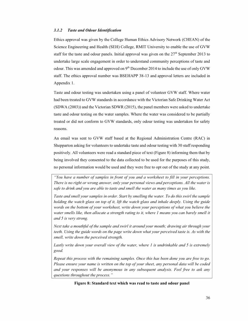
Figure 8: Standard text which was read to taste and odour panel .......................................... 36

Figure 9: Taste and odour panel worksheet ........................................................................... 38

Figure 10: Geosmin and MIB detections from the raw and final waters at Euroa WTP between

December 2014 and June 2016 .............................................................................................. 47

Figure 11: Free chlorine residual between December 2009 and October 2016 taken from the

disinfection point pre-CWS and the sample point at the outlet of the CWS. ......................... 48

Figure 12: Ranges of free chlorine residual at reticulation points in Euroa based on five years

data taken from the GVW compliance monitoring program ................................................. 49

Figure 13: The count of earthy /musty and chlorine odours detected correlated to related

SUVA values ......................................................................................................................... 50

Figure 14: The count of chlorine and earthy /musty odours detected in comparison to the UV

absorbance and odour detections ........................................................................................... 51

Figure 15: SUVA with respect to UV absorbance ................................................................. 52

Figure 16: The count of chlorine and earthy /musty odours detected with respect to DOC. . 52

Figure 17: SUVA with respect to DOC ................................................................................. 53

Figure 18: The count of chlorine and earthy /musty odours detected as a function of free

chlorine at the inlet and outlet of the CWS ............................................................................ 54

Figure 19: Correlation between the count of earthy /musty odours and total trihalomethanes

............................................................................................................................................... 55

12

Figure 20: EEM spectra from 15/2/2017 of (a) raw water inlet /Mountain Hut Reservoir (b)

Abbinga Reservoir and (c) Waterhouse Reservoir................................................................. 59

Figure 21: Volumes determined for each of the EEM spectral regions using the Chen et al

(2003) method ........................................................................................................................ 59

Figure 22: Raw Water Sample from Euroa WTP (Taken 15/02/2017).................................. 61

Figure 23: Relationship between raw DOC and UV absorbance ........................................... 61

Figure 24: EEMS volume make-up of eleven raw water samples in each region based on the

FRI technique method detailed by Chen et al (2003) ............................................................ 62

Figure 25: Reduction in DOC (a) and UVA (b) across the treatment process ....................... 63

Figure 26: EEM spectral volumes across the WTP process on the 6/5/2015 (a) and the

20/5/2015 (b) .......................................................................................................................... 64

Figure 27: Comparison of aluminium sulphate dose rates (a) and caustic soda dose rates (b)

............................................................................................................................................... 66

Figure 28: Ferric sulphate (a) and caustic soda (b) jar tested dose rates ................................ 67

Figure 29: ACH jar tested dose rates. .................................................................................... 68

Figure 30: EEM volumes from the raw water (a), the WTP (b), aluminium sulphate jar tests

(c), ferric sulphate jar tests (d) and ACH jar tests (e) ............................................................ 71

Figure 31: Organic carbon detection (OCD) outputs for liquid chromatography .................. 73

Figure 32: UV Detection (UVD) outputs at 254 nm from liquid chromatography ................ 74

Figure 33: EEM spectra for the samples used in Section 5.2.4.1 ........................................... 75

Figure 34: Chemical Cost per ML of Water Produced in 2014 including the Monthly Rainfall

............................................................................................................................................... 82

Figure 35: The average chemical cost determined based on jar tests and the WTP dose rates

............................................................................................................................................... 83

Figure 36: The combined financial assessment based on the impacts of each coagulant

assessed .................................................................................................................................. 87

Figure 37: CO2 emissions determined for each coagulant based on the delivery distance of

180 km and sludge disposal distance of 5.3 km each direction ............................................. 90

Figure 38: Overall findings from the environmental assessment ........................................... 91

Figure 39: Summary of the findings from the social impact assessment ............................... 96

13

Figure 40: Summary of the outputs from the economic, environmental and social assessment

............................................................................................................................................... 96

Figure 41: Outcomes from the sensitivity analysis ................................................................ 98

14

List of Tables

Table 1: A description of the nature of NOM with respect to the SUVA values and the impact

on coagulation (Edzwald & Tobiason, 1999) ........................................................................ 28

Table 2: Descriptions of the fractions obtained from LC-OCD (Rutlidge, et al., 2015) ........ 30

Table 3: Sampling locations used for taste and odour testing ................................................ 37

Table 4: Descriptors used as part of the triple bottom line assessment.................................. 42

Table 5: Weightings used in the triple bottom line assessment ............................................. 42

Table 6: Weightings used to undertake a sensitivity analysis to test the outcomes of the TBL

assessment .............................................................................................................................. 42

Table 7: Raw chemical costs taken from the GVW chemical contract .................................. 43

Table 8: Observed and expected odour counts determined by the taste and odour panel ...... 45

Table 9: Observed and expected values from taste testing panels ......................................... 46

Table 10: Pearson’s correlation coefficient determined between free chlorine residual and the

count of odours. ..................................................................................................................... 54

Table 11: Water quality parameters for Raw water inlet /Mountain Hut, Waterhouse and

Abbinga Reservoirs (n = 16) .................................................................................................. 57

Table 12: EEMs regions used in the fluorescence regional integration technique (taken from

Chen, et al., (2003)) ............................................................................................................... 58

Table 13: The DOC, UVA and SUVA values associated with the raw water samples treated

to EEMs ................................................................................................................................. 58

Table 14: Average and standard deviation of NOM indicators ............................................. 60

Table 15: Parameters for the samples subjected to EEMs ..................................................... 64

Table 16: A comparison of DOC removal rates as percentage between the WTP and the

alternative coagulants ............................................................................................................. 69

Table 17: A comparison of UVA reduction rates in percentage between the WTP and the

alternative coagulants. ............................................................................................................ 70

Table 18: The dates, DOC, UVA and SUVA values from the samples with EEMs determined

............................................................................................................................................... 70

Table 19: DOC and UVA values of the variously treated samples which had further organic

analysis ................................................................................................................................... 72

15

Table 20: The detected disinfection by product formation from chlorinated WTP and jar tested

samples against the DOC percentage removal ....................................................................... 75

Table 21: Raw water parameters for the jar tests used in determining sludge volumes ........ 76

Table 22: Measured sludge volumes shown in cm3 /2 L Jar .................................................. 77

Table 23: Volumes of bentonite suspension added and the resultant turbidity value ............ 77

Table 24: Count of odours detected against each coagulant following jar tests. ................... 78

Table 25: Chi squared statistic and the null hypotheses based on odours detected ............... 78

Table 26: Annual estimated chemical costs and associated savings ...................................... 84

Table 27: Annual estimated disposal costs with the volume of sludge produced .................. 84

Table 28: Financial assessment based on the determined annual chemical costs .................. 85

Table 29: Financial scores based on the GVW infrastructure program ................................. 86

Table 30: Environmental impacts associated with landfill disposal ...................................... 88

Table 31: Annual chemical volume requirements and annual delivery requirements ........... 89

Table 32: Scores Associated with the Environmental Assessment based on CO2 Emissions 90

Table 33: Outcomes of the assessment concerning the impacts improved taste and odour would

have on the community .......................................................................................................... 92

Table 34: Social assessment based on employee satisfaction ................................................ 94

Table 35: Social assessment based on direct operator impact ............................................... 95

16

Abbreviations

ABBREVIATION DESCRIPTION

ACH Aluminium chlorohydrate

ADWG Australian Drinking Water Guidelines

C.t Time of the chlorine in contact with the water

CAPEX Capital expenditure

CHEAN College Health Ethics Advisory Network

CWS Clear water storage

DBP Disinfection by products

DOC Dissolved organic carbon

EEM Excitation emission matrix

ESC Essential Services Commission

FPA Flavour profile analysis

FRI Fluorescence regional integration (technique)

FTT Taste/ flavour threshold test

GAC Granular activated carbon

GHG Greenhouse gases

GVW Goulburn valley water

HAA Haloacetic acid

HDPE High density polyethylene

HOC Hydrophobic organic carbon

LC-OCD Liquid chromatography – organic carbon detection

LMW Low molecular weight

MIB 2- Methylisoborneol

ML Mega-litre

NATA National Association of Testing Authorities, Australia

NOM Natural organic matter

ODT Odour detection threshold

Ofwat Water Services Regulatory Authority (Office of Water)

OPEX Operational expenditure

PAC Powdered activated carbon

RAC Regional administration centre

rpm Revolutions per minute

SCADA Supervisory control and data acquisition

SDWA Safe drinking water act

17

SDWR Safe drinking water regulations

SEC Size exclusion chromatography

SEH Science, Engineering and Health

SUVA Specific UV absorbance

TBL Triple bottom line

THM Trihalomethane

TOC Total organic carbon

TON Threshold odour number

UV Ultraviolet

UVA UV absorbance

UVT UV transmittance

WICS Water Industry Commission of Scotland

WTP Water treatment plant

w/w Weight per weight

w/v Weight per volume

18

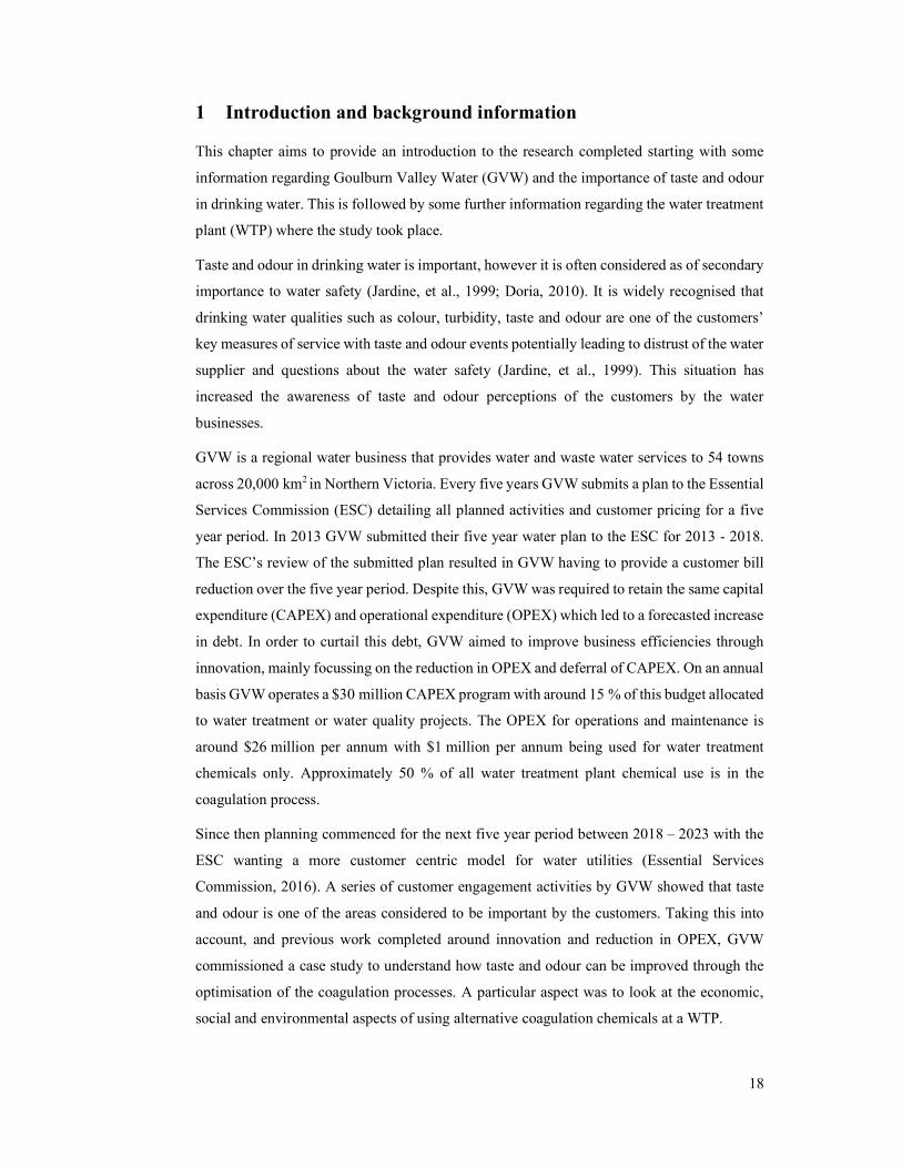
1 Introduction and background information

This chapter aims to provide an introduction to the research completed starting with some

information regarding Goulburn Valley Water (GVW) and the importance of taste and odour

in drinking water. This is followed by some further information regarding the water treatment

plant (WTP) where the study took place.

Taste and odour in drinking water is important, however it is often considered as of secondary

importance to water safety (Jardine, et al., 1999; Doria, 2010). It is widely recognised that

drinking water qualities such as colour, turbidity, taste and odour are one of the customers’

key measures of service with taste and odour events potentially leading to distrust of the water

supplier and questions about the water safety (Jardine, et al., 1999). This situation has

increased the awareness of taste and odour perceptions of the customers by the water

businesses.

GVW is a regional water business that provides water and waste water services to 54 towns

across 20,000 km2 in Northern Victoria. Every five years GVW submits a plan to the Essential

Services Commission (ESC) detailing all planned activities and customer pricing for a five

year period. In 2013 GVW submitted their five year water plan to the ESC for 2013 - 2018.

The ESC’s review of the submitted plan resulted in GVW having to provide a customer bill

reduction over the five year period. Despite this, GVW was required to retain the same capital

expenditure (CAPEX) and operational expenditure (OPEX) which led to a forecasted increase

in debt. In order to curtail this debt, GVW aimed to improve business efficiencies through

innovation, mainly focussing on the reduction in OPEX and deferral of CAPEX. On an annual

basis GVW operates a $30 million CAPEX program with around 15 % of this budget allocated

to water treatment or water quality projects. The OPEX for operations and maintenance is

around $26 million per annum with $1 million per annum being used for water treatment

chemicals only. Approximately 50 % of all water treatment plant chemical use is in the

coagulation process.

Since then planning commenced for the next five year period between 2018 – 2023 with the

ESC wanting a more customer centric model for water utilities (Essential Services

Commission, 2016). A series of customer engagement activities by GVW showed that taste

and odour is one of the areas considered to be important by the customers. Taking this into

account, and previous work completed around innovation and reduction in OPEX, GVW

commissioned a case study to understand how taste and odour can be improved through the

optimisation of the coagulation processes. A particular aspect was to look at the economic,

social and environmental aspects of using alternative coagulation chemicals at a WTP.

19

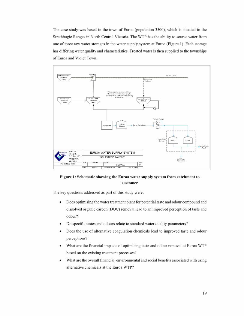
The case study was based in the town of Euroa (population 3500), which is situated in the

Strathbogie Ranges in North Central Victoria. The WTP has the ability to source water from

one of three raw water storages in the water supply system at Euroa (Figure 1). Each storage

has differing water quality and characteristics. Treated water is then supplied to the townships

of Euroa and Violet Town.

Figure 1: Schematic showing the Euroa water supply system from catchment to

customer

The key questions addressed as part of this study were;

Does optimising the water treatment plant for potential taste and odour compound and

dissolved organic carbon (DOC) removal lead to an improved perception of taste and

odour?

Do specific tastes and odours relate to standard water quality parameters?

Does the use of alternative coagulation chemicals lead to improved taste and odour

perceptions?

What are the financial impacts of optimising taste and odour removal at Euroa WTP

based on the existing treatment processes?

What are the overall financial, environmental and social benefits associated with using

alternative chemicals at the Euroa WTP?

20

The WTP predominantly extracts water from the Mountain Hut Reservoir via a gravity

pipeline, Mountain Hut Reservoir in turn is gravity fed from the Waterhouse Reservoir or from

Gooram Weir.

Waterhouse Reservoir is fed from Mountain Hut Creek which is often dry. Because of this,

heavy rainfall in the catchment area can significantly deteriorate water quality in a short period

of time due to the deposits of organic matter into the Reservoir. It is a large deep reservoir in

a predominantly forested area. There is significant vegetation around the reservoir and it has

been known to have algal blooms in the summer. The storage has a high organic content and

following rainfall it can experience a decrease in dissolved oxygen which has resulted in the

water having prominent odours.

Gooram Weir is located on the Seven Creeks just above Gooram Falls. The Seven Creeks

system is a relatively large network of smaller tributaries feeding into Seven Creeks. Polly

McQuinns dam on Seven Creeks is used to provide some water quality buffering prior to the

Gooram weir.

A third off stream storage, Abbinga Reservoir (300 ML), is located below Mountain Hut

Reservoir and can be used to supply the plant via Mountain Hut Reservoir. Abbinga Reservoir

is used during peak summer demand to supplement low flows in the catchment or when poor

water quality in Waterhouse renders it untreatable. The area of influence around Abbinga

Reservoir is mixed rotational farming between sheep and annual crops.

The raw water entering the water treatment plant is from Mountain Hut Reservoir which is a

mix of Waterhouse and Abbinga Reservoirs. The raw water is gravity fed to site and

coagulated using aluminium sulphate, with coagulation pH adjusted using caustic soda and a

flocculation aid added prior to entering a single sludge reactor clarifier. Due to the nature of

the raw water, during periods of low turbidity and high colour the floc produced can be light

resulting in an unstable sludge blanket. The clarifier is designed to operate with a thick sludge

blanket and ideally de-sludges at the same rate at which floc is created. In the past there have

been instances when the de-sludge rate has been too low and with the floc being light due to

the low turbidity, the sludge blanket has risen causing floc to pass onto the filter bed. This floc

deposit has then overloaded the filters placing the site at risk of protozoa breakthrough. In

order to overcome this, it has become common practice for the operators to purposely overdose

with coagulant. This practice increases the overall cost of treatment and can cause other issues

such as elevated aluminium residuals in the reticulation system. Prior to 2015, aluminium was

a scheduled item in the Victorian Safe Drinking Water Regulations (SDWR) but has

subsequently been removed following a review.

21

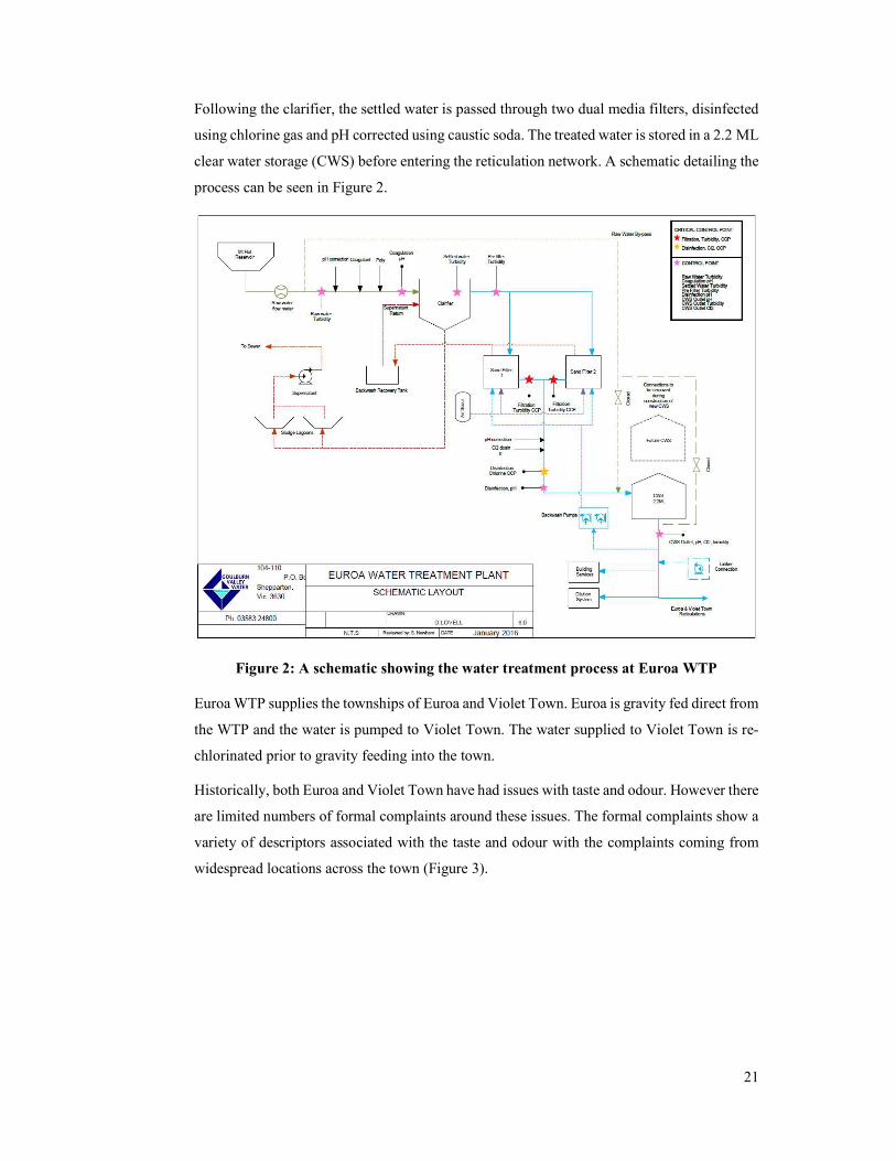
Following the clarifier, the settled water is passed through two dual media filters, disinfected

using chlorine gas and pH corrected using caustic soda. The treated water is stored in a 2.2 ML

clear water storage (CWS) before entering the reticulation network. A schematic detailing the

process can be seen in Figure 2.

Figure 2: A schematic showing the water treatment process at Euroa WTP

Euroa WTP supplies the townships of Euroa and Violet Town. Euroa is gravity fed direct from

the WTP and the water is pumped to Violet Town. The water supplied to Violet Town is re-

chlorinated prior to gravity feeding into the town.

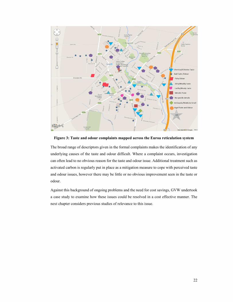
Historically, both Euroa and Violet Town have had issues with taste and odour. However there

are limited numbers of formal complaints around these issues. The formal complaints show a

variety of descriptors associated with the taste and odour with the complaints coming from

widespread locations across the town (Figure 3).

22

Figure 3: Taste and odour complaints mapped across the Euroa reticulation system

The broad range of descriptors given in the formal complaints makes the identification of any

underlying causes of the taste and odour difficult. Where a complaint occurs, investigation

can often lead to no obvious reason for the taste and odour issue. Additional treatment such as

activated carbon is regularly put in place as a mitigation measure to cope with perceived taste

and odour issues, however there may be little or no obvious improvement seen in the taste or

odour.

Against this background of ongoing problems and the need for cost savings, GVW undertook

a case study to examine how these issues could be resolved in a cost effective manner. The

next chapter considers previous studies of relevance to this issue.

23

2 Literature review

In this chapter previous studies related to the research were reviewed. The first section takes

into consideration customers’ views of taste and odour in drinking water and their increasing

role in water planning. The second section reviews water chemistry with a particular focus on

natural organic matter (NOM) and its interaction with disinfection processes. This is followed

up by an appraisal of research into chemical coagulation and its optimisation for NOM

removal. The final section looks at the role of cost benefit analysis in drinking water

management, and in particular, the use of Triple Bottom Line assessments as a decision

making tool.

2.1 The role of the customer in taste and odour management in drinking water

Over the last decade there has been an increased interest in involving customers in the

provision of drinking water (Doria, 2010). The most recent example of customer involvement

in drinking water management was in the United Kingdom’s (U.K) 2014 pricing

determination. This process put a large emphasis on customer engagement, putting the

customer values at the centre of decision making as a key part of the planning process (The

Water Services Regulatory Authority, 2011; Water Industry Commission of Scotland, 2015).

In Victoria, Australia, the ESC took note of the work completed by the Water Services

Regulatory Authority (Ofwat) and the Water Industry Commission of Scotland (WICS) and

included similar requirements for customer engagement in the pricing determination planning

process (Benvenuti, 2011; Essential Services Commission, 2015).

In most circumstances, customers have minimal interaction with their water supplier, tending

to only contact them when there is an issue (Water Industry Commission of Scotland, 2015).

Past research has shown that for every formal complaint, there are around 20 people with

issues who don’t and although this group of people represent the majority of dissatisfied

customers, there is limited research which understands the reasoning behind this (Chebat, et

al., 2005). Therefore the use of customer engagement as part of the planning process for the

Victorian water sector ensures the customer needs and values become integral to the ongoing

performance of the water business with the aim of reducing complaints and increasing

customer satisfaction (Essential Services Commission, 2016).

As mentioned in Chapter 1, customers measure the service of their water supplier through the

experience at their taps. Water quality parameters such as colour, turbidity, taste and odour

are the key indicators to the consumer of water safety (McGuire, 1995; Dietrich, 2006; Doria,

2010; Proulx, et al., 2010). Additionally these parameters are one of the main reasons

customers choose alternatives for drinking (Dietrich, 2006; Doria, 2006; Doria, et al., 2009;

24

Rodrigo, et al., 2009; Doria, 2010). As mentioned aesthetic parameters, including the taste and

odour, are normally considered by water suppliers as a secondary measure in drinking water

after drinking water safety or water supply (Bruchet, et al., 2004). However, taste and odour

in drinking water can be used to identify potential problems which may stem from issues with

the raw water such as contamination or algal activity, inadequacies with the existing water

treatment process, or issues with the distribution system (Watson, 2004; Doria, 2010).

Therefore monitoring taste and odours throughout the water treatment process allows water

companies to identify where a taste and odour issue may occur and to mitigate this accordingly

(Watson, 2004).

A notable taste and odour event was in 1994 in the Midlands of the UK. Contamination

occurred in the raw water and passed through the existing WTP without being identified. This

incident resulted in causing a direct impact on 110,000 customers, however the compounds

identified as being the cause were considered as having aesthetic properties only. Following

the incident, a study showed there were a number of resulting psychosomatic health issues

within the affected community (Fowle, et al., 1996, Furness, 2004). This incident resulted in

the water company being prosecuted for “supplying water not fit for consumption” with the

ruling judge deciding that the water was considered to be unfit if the customer did not like the

taste (Furness, 2004). This ruling is considered as a good reminder to water companies why

taste and odour should be considered as more than an aesthetic issue and used as a critical

parameter in the management of drinking water (Fowle, et al., 1996; Jardine, et al., 1999;

Furness, 2004).

2.2 Causes and removal of taste and odour in drinking water

Taste and odour in drinking water can result from a number of sources and all have the ability

to impact the overall flavour of the water in different ways (Burlingame, et al., 2017;

Antonopoulou, et al., 2014). There are four basic taste sensations (salty, sweet, bitter and sour)

with a fifth taste sensation (umami) more recently being recognised (Comrie, et al., 2002;

Dietrich, 2006; Burlingame, et al., 2007; Burlingame, et al., 2017). These tastes, in

conjunction with the odour of the water, make up the overall flavour of the water which is

normally what a consumer would refer to as taste (Twort, et al., 2000; Burlingame, et al.,

2017).

In the majority of cases most taste and odour issues occur from naturally occurring materials

in the raw water (Suffet, et al., 1999; Bae, et al., 2002; Ortenberg & Telsch, 2003; Doria, 2006;

Burlingame, et al., 2007). Raw water quality can be changeable and is dependent on a number

of factors such as weather patterns or river flows. The changeability of the raw water quality

results in fleeting or inconsistent taste and odour issues. This then leads to water companies

25

being unable to identify the odorous compound resulting in inadequate treatment being put in

place (Tondelier, et al., 2008).

Where taste and odours occur in the raw water, the cause can often be traced back to land

development in and around catchments. These catchments are individual ecosystems with the

microbial, plant and animal life all having the ability to impact the taste and odour in the water

(Twort, et al., 2000; Dietrich, 2006). Contamination of the water source may occur from both

point and diffuse sources. Diffuse sources of contamination may be from soil or the geology

of the area, whereas direct sources around the catchment area may include run off from

surrounding land increasing plant detritus or chemical contaminants in the water (Lin, 1977;

Wnorowski, 1992; Twort, et al., 2000).

The decay of vegetation within catchment areas has been known to cause odours. During the

decay process, a complex mixture of organic compounds is released (Lin, 1977). These

compounds are not only odorous in their own right but can cause the growth of other odour

producing organisms such as algae which can then release odorous metabolites (Lin, 1977;

Wnorowski, 1992; Ortenberg & Telsch, 2003; Dietrich, 2006)

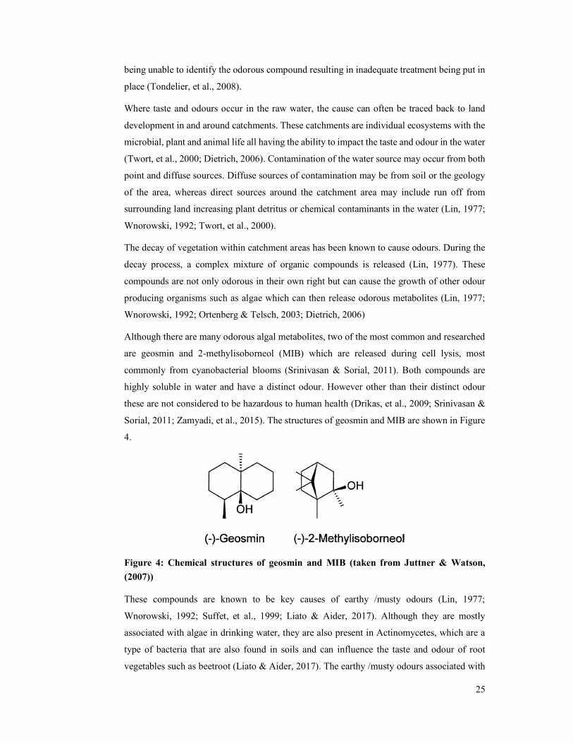
Although there are many odorous algal metabolites, two of the most common and researched

are geosmin and 2-methylisoborneol (MIB) which are released during cell lysis, most

commonly from cyanobacterial blooms (Srinivasan & Sorial, 2011). Both compounds are

highly soluble in water and have a distinct odour. However other than their distinct odour

these are not considered to be hazardous to human health (Drikas, et al., 2009; Srinivasan &

Sorial, 2011; Zamyadi, et al., 2015). The structures of geosmin and MIB are shown in Figure

4.

Figure 4: Chemical structures of geosmin and MIB (taken from Juttner & Watson,

(2007))

These compounds are known to be key causes of earthy /musty odours (Lin, 1977;

Wnorowski, 1992; Suffet, et al., 1999; Liato & Aider, 2017). Although they are mostly

associated with algae in drinking water, they are also present in Actinomycetes, which are a

type of bacteria that are also found in soils and can influence the taste and odour of root

vegetables such as beetroot (Liato & Aider, 2017). The earthy /musty odours associated with

26

geosmin and MIB can be detected down to concentrations as low as 10 ng/L which means that

there may be resultant customer complaints associated with the presence of these compounds

in drinking water (Jung, et al., 2004; Drikas, et al., 2009). Both of these compounds are

difficult to remove through traditional water treatment processes with the removal efficiency

being as low as 20% due to their small size (Jung, et al., 2004; Zamyadi, et al., 2015). In

general oxidation or adsorption are required to remove both geosmin and MIB, with the use

of powdered and granular activated carbon (PAC and GAC, respectively) being a common

and effective adsorbent (Drikas, et al., 2009; Zamyadi, et al., 2015). However, the presence of

NOM at levels of 3- 10 mg/L DOC in water has been shown to decrease the efficiency of the

removal of MIB and geosmin through adsorption onto activated carbon. This difficulty is due

to the comparative size of the NOM molecules utilising the surface of the carbon in place of

the smaller geosmin and MIB molecules (Srinivasan & Sorial, 2011). Oxidation of geosmin

and MIB is a more effective method of removal, with both geosmin and MIB being

successfully removed through the use of ozone, hydrogen peroxide (H2O2) and ultraviolet

(UV) light. There are disadvantages to using these as they can be expensive, associated

disinfection by-products (DBPs) can form, and residual chemicals may remain within the

water following oxidation which may require further removal or treatment (Srinivasan &

Sorial, 2011; Zamyadi, et al., 2015), and some of which may also cause odours (Bruchet, et

al., 2004).

In addition to odorous compounds being present in the raw water, organic compounds released

as a result of decaying vegetation can react with disinfectants at the WTP to create odorous

compounds (Bruchet, et al., 2004; Dietrich, 2006; Deborde & Van Gunten, 2008; McDonald,

et al., 2009). In Australia the most common disinfection chemical employed is chlorine, which

is also one of the most commonly cited causes of taste and odour issues with drinking water

from customers (McDonald, et al., 2013; McDonald, et al., 2009; Piriou, et al., 2004). As well

as being used for pathogen control, chlorine can be used to control taste and odour compounds

through oxidation, or by masking odour compounds (Bruchet, et al., 2004; Lin, 1977).

However, in the event that the control of taste and odours is not completely effective, any

odours that may have been masked can recur once the free chlorine residual dissipates

(Dietrich, et al., 1995; Bruchet, et al., 2004; Deborde & Van Gunten, 2008; McDonald, et al.,

2009). Hence, where there are variable chlorine levels within a water supply, there is the

potential for taste and odour complaints to occur (Puget, et al., 2010; McDonald, et al., 2013).

Given the nature of taste and odour causing compounds it is expected that there are few water

sources which are free from taste and odours, thus treatment will normally be required in order

to provide palatable drinking water (Wnorowski, 1992; Ortenberg & Telsch, 2003; Watson,

2004). Treatment of taste and odours can be difficult using traditional treatment processes

27

(coagulation, sedimentation, filtration, chlorination) depending on the characteristics of the

taste and odour causing compounds. One of the more effective approaches to the treatment of

taste and odours is a multiple-barrier approach (Wnorowski, 1992; Doria, 2010). It can be

useful to identify the taste and odour causing compounds prior to treatment, though this is not

always practical or possible. Therefore trial and error is often an appropriate method to

determine the best approach when used in conjunction with odour testing through the process

(Wnorowski, 1992).

2.2.1 Detection of taste and odours in drinking water

The organoleptic detection of taste and odours in drinking water is subjective and the task of

identifying an unacceptable level through analytical techniques for each chemical in different

waters can be nearly impossible. Many taste and odour causing compounds are detectable by

the human nose down to a few ng/L (Bae, et al., 2002; Burlingame, et al., 2017). For this

reason the most common method of taste and odour detection is to use consumer and trained

panels to assess drinking water flavour and odour (Doria, 2010; Burlingame, et al., 2017).

The simplest methods of using people (either trained or untrained) to determine tastes and

odours is the Flavour Profile Analysis (FPA) technique. This technique involves the

examination of the sensory characteristics to identify the full range of tastes and odours

associated with each sample (Bartels, et al., 1986; Suffet, et al., 1999; Burlingame, et al.,

2017). The most common method of detecting tastes and odour in drinking water is the

Threshold Odour Number test (TON) and the Taste or Flavour Threshold Test (FTT). These

methods involve the dilution of a sample to the lowest perceptible point of the taste or odour

(Ortenberg & Telsch, 2003; Burlingame, et al., 2017).

It is possible to utilise analytical testing for chemical parameters that cause odour, however

this can be costly for water companies, especially where the taste and odour cause is unknown

(McDonald, et al., 2009). Many taste and odour causing compounds are detectable by people

to below the level of detection of some analytical methods (Ortenberg & Telsch, 2003;

McDonald, et al., 2009).

2.3 Water chemistry relating to natural organic matter

NOM is an overarching term which encompasses all organic matter present in fresh waters

and can be complex in its composition (Matilainen, et al., 2011). The quality of water

containing NOM is variable with no simple method to determine the overall structure of NOM

(Drikas, 2003). The use of simple water quality parameters can be useful to determine the

characteristics and therefore the treatability of the water (Matilainen, et al., 2011; Edzwald &

Kaminski, 2007). As the presence of NOM is the main cause of the brown colour some waters

display, the use of colour as a measurement of NOM can be useful (Matilainen, et al., 2011;

28

Fan, et al., 2001). Similarly the use of absorbance of UV light at 254 nm can be a useful

parameter to measure the concentration of organics present. However, the presence of other

UV absorbing materials such as iron and manganese can influence the colour and are also

absorbed at 254 nm which may lead to a non-representative view of the NOM present

(Matilainen, et al., 2011). TOC and DOC are useful for providing an overview of the entire

mixture of NOM within the water source where TOC is the sum of the particulate and DOC

(Matilainen, et al., 2011). Although the use of all these parameters is relatively easy and can

be completed fairly quickly by an operator, the disadvantage is that they only give an

indication of the concentration of organics present and very little about their characteristics

(Matilainen, et al., 2011; Matilainen, et al., 2010).

Specific UV absorbance (SUVA) can be used as an indicator of the nature of the NOM and

the effectiveness of the NOM removal through coagulation (Edzwald & Tobiason, 1999;

Matilainen, et al., 2011). SUVA is the normalisation of the ultraviolet absorbance at 254 nm

(UVA) against the DOC (Edzwald & Tobiason, 1999; Matilainen, et al., 2011). The SUVA

values may describe the nature of the NOM in water with respect to hydrophobicity,

aromaticity and molecular weight as well as the potential effectiveness of NOM removal

through coagulation (Tan, et al., 2005; Matilainen, et al., 2011).

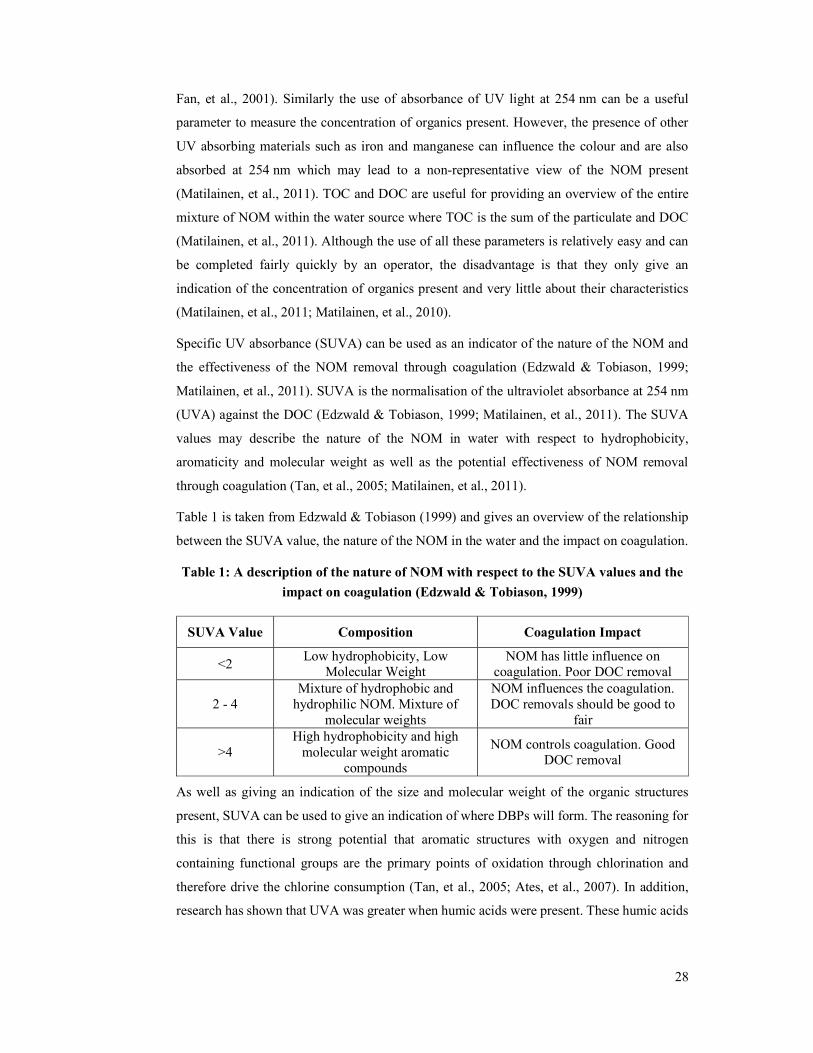
Table 1 is taken from Edzwald & Tobiason (1999) and gives an overview of the relationship

between the SUVA value, the nature of the NOM in the water and the impact on coagulation.

Table 1: A description of the nature of NOM with respect to the SUVA values and the

impact on coagulation (Edzwald & Tobiason, 1999)

SUVA Value Composition Coagulation Impact

<2 Low hydrophobicity, Low

Molecular Weight NOM has little influence on

coagulation. Poor DOC removal

2 - 4 Mixture of hydrophobic and

hydrophilic NOM. Mixture of molecular weights

NOM influences the coagulation. DOC removals should be good to

fair

>4 High hydrophobicity and high

molecular weight aromatic compounds

NOM controls coagulation. Good DOC removal

As well as giving an indication of the size and molecular weight of the organic structures

present, SUVA can be used to give an indication of where DBPs will form. The reasoning for

this is that there is strong potential that aromatic structures with oxygen and nitrogen

containing functional groups are the primary points of oxidation through chlorination and

therefore drive the chlorine consumption (Tan, et al., 2005; Ates, et al., 2007). In addition,

research has shown that UVA was greater when humic acids were present. These humic acids

29

tended to form higher concentrations of trihalomethanes (THMs) and haloacetic acids (HAAs)

than the fulvic acids present in the same source water (Ates, et al., 2007).

Most water sources have a mixture of hydrophobic and hydrophilic organic content with

almost half of the organic content being attributed to hydrophobic humic substances (humic

and fulvic acids) which tend to have a greater molecular weight (Fan, et al., 2001; Matilainen,

et al., 2010). The remaining non humic organic content is made up of proteins amino acids

and carbohydrates. This fraction of organic content tends to be less hydrophobic (Fan, et al.,

2001). The non-humic matter is more difficult to remove through coagulation, as it tends to

be smaller in size and have a low charge density (Matilainen, et al., 2010). The differences in

size and properties of all organic matter present in source waters impacts on the treatability of

the water by coagulation, the chlorine demand for effective disinfection and the potential for

DBP formation.

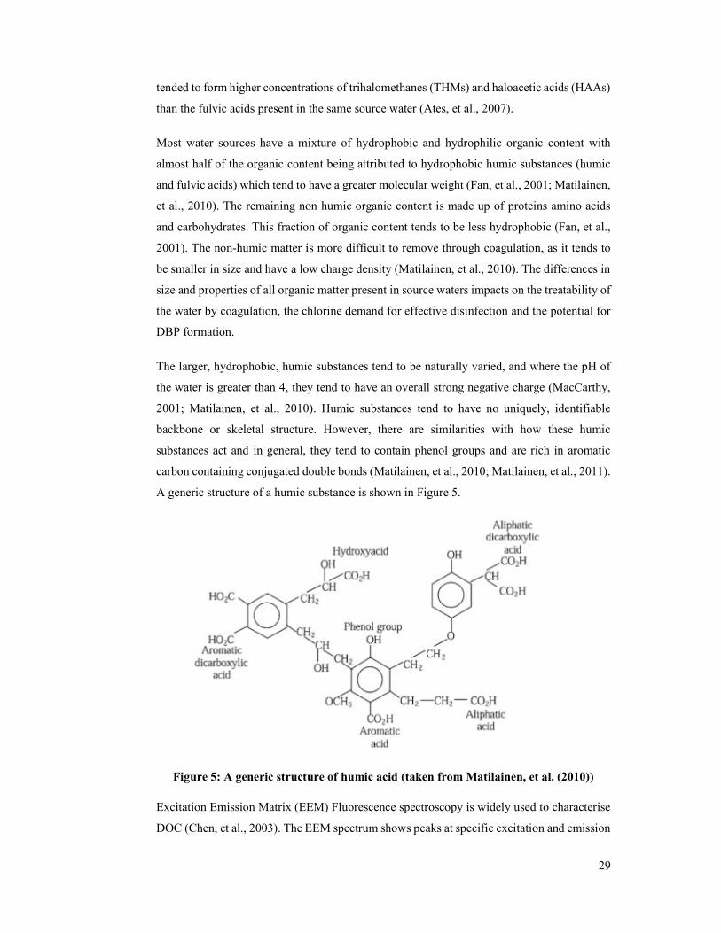
The larger, hydrophobic, humic substances tend to be naturally varied, and where the pH of

the water is greater than 4, they tend to have an overall strong negative charge (MacCarthy,

2001; Matilainen, et al., 2010). Humic substances tend to have no uniquely, identifiable

backbone or skeletal structure. However, there are similarities with how these humic

substances act and in general, they tend to contain phenol groups and are rich in aromatic

carbon containing conjugated double bonds (Matilainen, et al., 2010; Matilainen, et al., 2011).

A generic structure of a humic substance is shown in Figure 5.

Figure 5: A generic structure of humic acid (taken from Matilainen, et al. (2010))

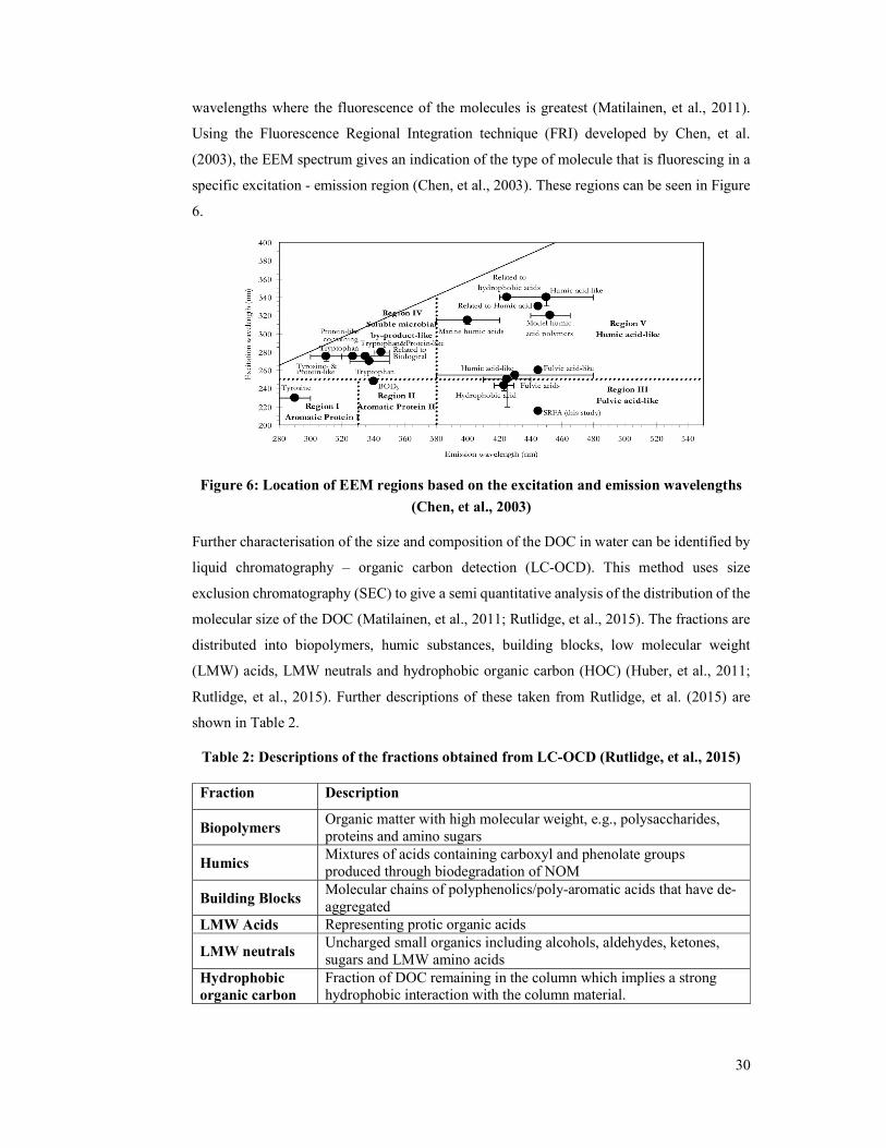
Excitation Emission Matrix (EEM) Fluorescence spectroscopy is widely used to characterise

DOC (Chen, et al., 2003). The EEM spectrum shows peaks at specific excitation and emission

30

wavelengths where the fluorescence of the molecules is greatest (Matilainen, et al., 2011).

Using the Fluorescence Regional Integration technique (FRI) developed by Chen, et al.

(2003), the EEM spectrum gives an indication of the type of molecule that is fluorescing in a

specific excitation - emission region (Chen, et al., 2003). These regions can be seen in Figure

6.

Figure 6: Location of EEM regions based on the excitation and emission wavelengths

(Chen, et al., 2003)

Further characterisation of the size and composition of the DOC in water can be identified by

liquid chromatography – organic carbon detection (LC-OCD). This method uses size

exclusion chromatography (SEC) to give a semi quantitative analysis of the distribution of the

molecular size of the DOC (Matilainen, et al., 2011; Rutlidge, et al., 2015). The fractions are

distributed into biopolymers, humic substances, building blocks, low molecular weight

(LMW) acids, LMW neutrals and hydrophobic organic carbon (HOC) (Huber, et al., 2011;

Rutlidge, et al., 2015). Further descriptions of these taken from Rutlidge, et al. (2015) are

shown in Table 2.

Table 2: Descriptions of the fractions obtained from LC-OCD (Rutlidge, et al., 2015)

Fraction Description

Biopolymers Organic matter with high molecular weight, e.g., polysaccharides, proteins and amino sugars

Humics Mixtures of acids containing carboxyl and phenolate groups produced through biodegradation of NOM

Building Blocks Molecular chains of polyphenolics/poly-aromatic acids that have de-aggregated

LMW Acids Representing protic organic acids

LMW neutrals Uncharged small organics including alcohols, aldehydes, ketones, sugars and LMW amino acids

Hydrophobic organic carbon

Fraction of DOC remaining in the column which implies a strong hydrophobic interaction with the column material.

31

Further quantification of the concentration of the dissolved organic fractions is completed

using organic carbon detection. LC-OCDs have been used successfully to characterise the

efficiency of water treatment processes in the past (Huber, et al., 2011; Matilainen, et al., 2011;

Rutlidge, et al., 2015).

2.3.1 Removal of natural organic matter using coagulation

The most common and effective method of NOM removal is through chemical coagulation

where the characteristics of the NOM influence the amount and type of chemical used (Jarvis,

et al., 2012; Soh, et al., 2008; Drikas, 2003). Coagulation and flocculation are two key

processes in drinking water treatment which are responsible for the removal of impurities such

as turbidity, colour, pathogens, organic and inorganic matter (Twort, et al., 2000; Ghernaout

& Ghernaout, 2012).

Chemical coagulation is the process where a positively charged coagulant is mixed thoroughly

with the raw water forming various complexes (floc), which are dependent upon on the

composition of the raw water (Twort, et al., 2000). Flocculation is the process where

aggregation of these complexes occurs to aid in removal through a clarification process

(Twort, et al., 2000; Ghernaout & Ghernaout, 2012). Traditionally chemical coagulation was

used as a method for removing larger pathogens, turbidity and colour, with more recent focus

being on NOM removal to decrease DBP formation and to reduce chlorine consumption (Soh,

et al., 2008). For removal of NOM an inorganic metal coagulant is most commonly used.

When added to water the metal salts are dissociated to form a positively charged ion which

hydrolyses and forms complexes with both particulate and soluble matter within the water

(Matilainen, et al., 2010; Jarvis, et al., 2012).

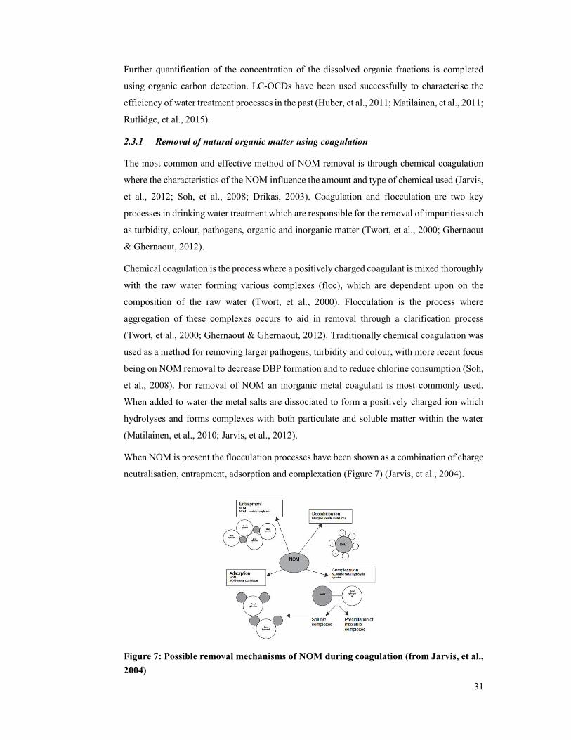
When NOM is present the flocculation processes have been shown as a combination of charge

neutralisation, entrapment, adsorption and complexation (Figure 7) (Jarvis, et al., 2004).

Figure 7: Possible removal mechanisms of NOM during coagulation (from Jarvis, et al.,

2004)

32

The removal mechanism that occurs is dependent upon the NOM composition including the

molecular size, functionality and hydrophobicity (Matilainen, et al., 2010; Jarvis, et al., 2004).

Further to this, even within the same water source the removal mechanism for the different

NOM molecules will vary (Jarvis, et al., 2004). There is evidence to suggest that where NOM

is present in high concentrations the floc produced is low density and weak in comparison to

flocs produced where turbidity is present (Jarvis, et al., 2012; Jarvis, et al., 2004). This can

lead to issues with solid – liquid separation (Jarvis, et al., 2012). The effectiveness of

coagulation to remove NOM is influenced by a range of factors including pH of the water,

alkalinity, chemical mixing and the properties of the NOM (Jarvis, et al., 2004; Matilainen, et

al., 2010).

The normal method of determining a coagulant dose is using the measures of turbidity and

colour as an indicator of effectiveness. However, the conditions for optimal turbidity and

colour removal are not necessarily the same as those for NOM removal (Matilainen, et al.,

2010). When considering coagulation for NOM removal, the dose and pH conditions need to

be considered more than for where the key parameter is turbidity removal (Jarvis, et al., 2004;

Matilainen, et al., 2010).

2.3.2 Interaction of natural organic matter with chlorine disinfection

As previously mentioned where residual NOM is present following the coagulation process,

there is potential for DBP formation. In Australia the most commonly formed DBPs are THMs

or HAAs (Fabris, et al., 2003; Korotta-Gamage & Sathasivan, 2017). DBPs form through a

reaction between NOM and chlorine that is applied for disinfection purposes, however the

mechanisms associated with the formation of DBPs is complex and are dependent upon many

factors (Ates, et al., 2007; Roccaro, et al., 2009). To add to the complexity, much research is

conflicting, particularly around the formation of HAAs (Bond, et al., 2012). In general the

presence of longer chained amino acids increases the HAA formation potential (Bond, et al.,

2012).

Other than the characteristics associated with the NOM within the water, the type of DBP

formed is dependent upon other parameters within the water such as pH, temperature, the

presence of bromide and contact time (Twort, et al., 2000; Gallard & von Gunten, 2002; Gang,

et al., 2003; Korotta-Gamage & Sathasivan, 2017). The influence of pH not only the impacts

on the potential for DBP formation but also the type formed. Research has shown that by

decreasing the pH prior to disinfection the formation of DBPs is lower, and conversely where

the pH is increased the formation of DBPs is higher (Mishra, et al., 2013). Additionally as the

pH increases from pH 7 to pH 11, there is a 30 % to 50 % increase in THM formation in

preference to HAAs (Mishra, et al., 2013). In general temperature increases see an increase in

33

the reaction of NOM with free chlorine, increasing the amount of DBPs being formed (Twort,

et al., 2000; Mishra, et al., 2013). There is some conflicting research around this, indicating

that there is not a linear relationship between temperature and THM formation. Garcia-

Villanova, et al. (1997) showed there is an optimum point for THM formation at 19°C after

which the concentration of THMs decreases (Garcia-Villanova, et al., 1997; Mishra, et al.,

2013).

The presence of bromide in raw water can impact on the types of DBP formed, especially the

ratios of bromide/DOC and bromide/chlorine (Ates, et al., 2007). During disinfection the

bromide is oxidised to form hypobromous acid which reacts readily with the residual NOM to

form brominated DBPs. As the ratio of chlorine to bromide increases the likelihood of

brominated DBPs is favoured (Twort, et al., 2000; Bond, et al., 2012; Mishra, et al., 2013).

The final key component that impacts on DBP formation is the chlorine concentration and the

contact /reaction time (Garcia-Villanova, et al., 1997; Mishra, et al., 2013). The general

opinion is that THM formation is dependent upon the concentration of the free chlorine.

Present and past research into this area has shown that there is a linear relationship between

chlorine demand and the production of THMs (Garcia-Villanova, et al., 1997). Research has

shown that the bulk of DBPs will form rapidly following the initial chlorine dose, with

minimal increase in DBPs being formed after 48 hours (Mishra, et al., 2013).

In Australia the concentration of DBPs is regulated on a state basis, however, in general the

levels of DBPs permitted in drinking water is higher than Europe or the USA. The regulatory

standards seen in these countries have led to a greater emphasis on NOM removal up front

(Edzwald & Tobiason, 1999; Jarvis, et al., 2012). The presence of NOM during the

disinfection process increases the consumption of chlorine required to achieve the same

pathogen kill rate. This in turn leads to the practice of increased chlorine doses being used,

thus increasing the DBP formation potential (Chang, et al., 2006).

It is clear that many factors affect taste and odour, and the removal of potentially taste and

odour causing materials. The Triple Bottom Line (TBL) analysis is considered as a useful

approach to assist in decision making in the selection of suitable treatment. This approach is

described in the next section.

2.4 The use of a triple bottom line assessment in the water industry

TBL assessment is a common tool used by businesses to measure the overall sustainability of

a project or as a tool for self-evaluation (Marques, et al., 2015). The TBL encompasses

financial, social and environmental aspects of the project or process being assessed (Slaper &

Hall, 2011). In the water sector the use of financial performance as a measure of commercial

viability was used during the ‘economic reform era’ of the 1980s and 1990s. The changes in

34

regulation of the economy resulted in changes to the governance around the urban water sector

(Infrastructure Partnerships Australia, 2015). Since this period the overall sustainability of the

sector was reviewed and the use of a multi-criteria assessment became common (Marlow, et

al., 2010; Adams, et al., 2014). Despite the industry’s efforts to assess the sustainability of a

project through the assessment of social, environmental and financial impacts, it has been

found that there is often a shortfall. This is mainly due to the stakeholders involved and their

conflicting priorities (Lundie, et al., 2006; Marques, et al., 2015). In both South Australia (SA)

and Western Australia (WA), the basic concepts of the TBL have been shifted slightly to take

into consideration time dimensions as well as political and technological dimensions (Lundie,

et al., 2006). As the services provided by the water industry underpin societal needs, the

industry is in a position to be a leader in sustainability and requires a holistic view (Lundie, et

al., 2006; Lai, et al., 2008; Marques, et al., 2015).

35

3 Methodology

This chapter details the approach taken for this research. The chapter consists of 3 sections,

Section 3.1 describes how the taste and odour issues were identified. Section 3.2 contains

information regarding the optimisation of the treatment process for taste and odour removal.

Section 3.3 discusses the method taken to complete the TBL assessment.

3.1 Identification of the taste and odour issues

This section details the process for the identification of the causes of taste and odours at Euroa

WTP. This was completed through the use of a taste and odour panel to identify the key taste

and odours in the water. The identified taste and odours were then correlated to water quality

data from the same period to understand any pertinent relationships

3.1.1 Water quality data analysis

Raw and final water quality data from 2004 to 2014 was obtained from the GVW Water

Quality database “Aquantify” and analysed. Data analysed was for the following parts of the

process:

Raw water;

WTP process data including post clarification and filtered waters;

Treated water prior to entry to town following disinfection; and,

The reticulated water.

Two sources of data were analysed, externally obtained data and field data. The external

laboratory data was obtained from SGS Laboratories, a NATA accredited laboratory which

uses Standard Methods for the Examination of Water and Wastewater. All field data analysed

was collected using GVW standard bench top testing equipment as per the manufacturer’s

guidelines.

External laboratory data included UV transmittance (UVT), DOC, TOC, THMs, HAAs and

iron and manganese contents. Field data comprised free and total chlorine, electrical

conductivity, turbidity, pH and true colour. Meta-analysis was undertaken to understand

seasonal variations and correlations to other water quality parameters.

Where no data was available, or the data was limited, a weekly program for further sampling

and testing was undertaken over the summer period of 2014/15. Characterisation was done by

SGS or in the field. Water was characterised at the raw water sources (Abbinga Reservoir,

Waterhouse Reservoir, Mountain Hut Reservoir /raw water inlet) as well as post clarification,

post filtration, and pre - and post - CWS following disinfection.

36

3.1.2 Taste and Odour Identification

Ethics approval was given by the College Human Ethics Advisory Network (CHEAN) of the

Science Engineering and Health (SEH) College, RMIT University to enable the use of GVW

staff for the taste and odour panels. Initial approval was given on the 27th September 2013 to

undertake large scale engagement in order to understand community perceptions of taste and

odour. This was amended and approved on 9th December 2014 to include the use of only GVW

staff. The ethics approval number was BSEHAPP 38-13 and approval letters are included in

Appendix 1.

Taste and odour testing was undertaken using a panel of volunteer GVW staff. Where water

had been treated to GVW standards in accordance with the Victorian Safe Drinking Water Act

(SDWA (2003)) and the Victorian SDWR (2015), the panel members were asked to undertake

taste and odour testing on the water samples. Where the water was considered to be partially

treated or did not conform to GVW standards, only odour testing was undertaken for safety

reasons.

An email was sent to GVW staff based at the Regional Administration Centre (RAC) in

Shepparton asking for volunteers to undertake taste and odour testing with 30 staff responding

positively. All volunteers were read a standard piece of text (Figure 8) informing them that by

being involved they consented to the data collected to be used for the purposes of this study,

no personal information would be used and they were free to opt out of the study at any point.

“You have a number of samples in front of you and a worksheet to fill in your perceptions. There is no right or wrong answer, only your personal views and perceptions. All the water is safe to drink and you are able to taste and smell the water as many times as you like.

Taste and smell your samples in order. Start by smelling the water. To do this swirl the sample holding the watch glass on top of it, lift the watch glass and inhale deeply. Using the guide words on the bottom of your worksheet, write down your perceptions of what you believe the water smells like, then allocate a strength rating to it, where 1 means you can barely smell it and 5 is very strong.

Next take a mouthful of the sample and swirl it around your mouth; drawing air through your teeth. Using the guide words on the page write down what your perceived taste is. As with the smell, write down the perceived strength.

Lastly write down your overall view of the water, where 1 is undrinkable and 5 is extremely good.

Repeat this process with the remaining samples. Once this has been done you are free to go. Please ensure your name is written on the top of your sheet, any personal data will be coded and your responses will be anonymous in any subsequent analysis. Feel free to ask any questions throughout the process.”

Figure 8: Standard text which was read to taste and odour panel

37

On a weekly basis not all volunteers were available to be involved in the panel due to prior

commitments. This meant that the panel composition changed on a weekly basis depending

on the availability of the participating GVW staff. On average each panel contained 13

participants. Of these 13, at least 6 of the members were the same each week.

One - litre samples of potable water were collected from GVW sampling locations supplied

by the Euroa WTP and a fourth sample was taken from the Regional Administration Centre

(RAC) in Shepparton as a control location (Table 3). The decision to use the Shepparton RAC

as a control was made as the panel were all based in this location and drink the water daily.

Therefore it was assumed that the perceptions of this water should be consistent against the

unknown samples from Euroa. The samples were tested on the same day of collection at room

temperature (between 18 and 23°C).

Table 3: Sampling locations used for taste and odour testing

Sample Sample Location 1 Euroa CWS 2 Euroa Reticulation System 3 Violet Town Reticulation System 4 Shepparton RAC

Approximately 30 mL of each sample was transferred into a tasting glass and covered with a

watch glass. Each sample was labelled with a non-identifiable tag to remove any pre-

conceived bias about the taste and odour of the sample location. These non-identifiable tags

changed weekly to remove any pre-conceptions.

Using the instructions given in Figure 8 the panel were asked to smell the samples firstly,

followed by tasting them. Samples that did not conform to water safety standards were

removed before taste testing but after all odour testing was complete to minimise bias. All

results were recorded on the pro-forma (Figure 9).

Each week the order of the samples was changed to remove any potential bias associated with

a particular sample. All data collected were recorded removing any personal identification.

38

Figure 9: Taste and odour panel worksheet

It was suspected that there were certain locations where particular tastes and odours were

strong and from this the null hypothesis was developed that the taste and odour of the sample

and the sample location were independent. The significance level used was p < 0.05.

The data analysed were collated and counted for each taste and odour detected against the

location. From this the expected number of taste and odour detections against each location

was determined using Equation 1. From this the Chi Squared value (X2) was able to be

determined using Equation 2

=

Equation 1

= ∑ ( ) Equation 2

Where specific odours were identified by the panel, the details from Suffet, et al. (1999) which

identifies specific odours from a chemical compound, was used to ascertain where a potential

chemical compound may be present. These compounds were identified and analysed with

respect to the odour detection thresholds (ODT).

The water quality parameters mentioned in section 3.1.1 were used to understand the

relationship to odour. The count of each odour detected was collated by month and compared

to the average water quality data of the same month. The seasonality of the water quality

parameters was consistent and therefore this approach was considered to be representative.

Where the relationships appeared to be linear, these were correlated using Pearson’s

correlation coefficient with a significance value of p < 0.05.

39

3.2 Optimisation of the treatment processes for taste and odour removal

Following the identification of the key taste and odour compounds, jar testing was completed

to understand the impact on odour removal. The existing chemical coagulant dosing was

reviewed and optimised for odour improvement. The optimisation targeted the water quality

parameters which were identified as relating to odours as determined in section 3.1.2.

Alternative chemical coagulants were trialled with respect to odour improvement.

3.2.1 Jar testing for taste and odour removal

Jar testing was completed using aluminium sulphate, aluminium chlorohydrate (ACH) and

ferric sulphate as coagulants. The method followed is detailed by Murray & Mosse (2015).

Coagulant stock solutions were made up at the beginning of each month based on the guidance

provided by Murray & Mosse (2015). Caustic soda stock solution was made using 3.65 mL of

46% caustic soda and made up to 250 mL with deionised water. Aluminium sulphate stock

solution was made using 16.25 mL of 47% aluminium sulphate and made up to 1000 mL with

deionised water. Ferric sulphate stock solution was made using 13.48 mL of 12 % ferric

sulphate and made up to 1000 mL with deionised water. ACH stock solution was made using

14.93 mL of 40% ACH and made up to 1000 mL with deionised water.

A four - jar Platypus jar testing system with 2 L beakers was used. It was set to operate at 120

rpm for 2 minutes to replicate flash mixing conditions at Euroa WTP, and 30 rpm for 20

minutes to replicate flocculation time and allow floc to form.

The jars were left for 20 minutes following flocculation to allow the floc formed to settle.

After settlement water was drawn from the top of the jar 5 cm below the surface, and the pH,

turbidity, true colour and UVA were determined using GVW standard instruments using

manufacturer’s instructions. These data were used to identify the most effective dose as

indicated by the lowest turbidity, colour and UVA.

Turbidity was determined by a HACH 2100 N turbidimeter in a 30 mm glass sample cell. pH

was determined in situ using a Eutech waterproof pH meter. Determination of true colour and

UVA required samples to be filtered through a 0.45 µm syringe filter. True colour was

determined using a HACH DR 2700 Spectrophotometer at 540 nm in a quartz cuvette with 50

mm path length. UVA was determined using a Realtech portable UV field meter at 254 nm in

a quartz cuvette with a path length of 10 mm. The Realtech Portable UV field meter has the

ability to give outputs of both UVT and UVA. UVT has a logarithmic relationship to UVA

and can be converted using Equation 3. Deionised water was used as a blank for UVA and

true colour.

UVA = 2 – log 10 (UVT) Equation 3

40

Further analysis of the most effective doses was completed by SGS Laboratories where DOC

and UVT were determined. These were then compared to the WTP performance post

clarification.

A 1 L graduated Imhoff cone was used to determine the volume of wet sludge in cm3/L. After

all the required supernatant samples had been removed after settling, the remaining one litre

was transferred to the Imhoff cone and allowed to settle for 20 minutes. The volume of wet

sludge was determined after this time using the graduations on the cone.

After completion of the jar tests, the odour of the most effective coagulant dose was

determined using the taste and odour testing panel from Section 3.1.2 and compared against

the odour from the WTP and the raw water. Data were analysed using the Chi squared statistic

(Section 3.1.2). As the water was not considered to be potable following the jar tests the panel

were asked to assess only the odour.

3.2.2 Fluorescence excitation-emission matrix spectra

Selected samples underwent further organic analysis using EEMs. This was to understand the

changes in the composition of organic matter following treatment.

All samples were filtered through a 0.45 µm filter and the fluorescence EEM spectra were

determined using a LS55 PerkinElmer Spectrometer over excitation and emission wavelength

ranges of 220–465 nm and 280–550 nm, respectively. The band width for both excitation and

emission was set at 5 nm. Data was analysed using the Fluorescence Regional Integration

(FRI) technique detailed in Chen et al. (2003).

Although the method outlined by Chen et al (2003) has been superseded by more accurate

techniques for interpreting EEM spectra, the FRI was considered to be sufficient for the

purposes of this study as it gave an indication of the volumes for each of the regions and thus

presence of the different fluorescent compounds.

3.2.3 Liquid Chromatography – Organic Carbon Detection

Following the jar test completed on the 28/4/2017, 50 mL of each sample was sent to the

Water Research Centre at the University of New South Wales. The molecular weight

distribution of the organic compounds in each sample was determined using a DOC-Labor

LC-OCD Model 8, with a Toyopearl TSK HW -50S Column. A phosphate buffer of pH 6.4

was used as the mobile phase.

41

3.2.4 Replication of post-coagulation chemical dosing in the jar tested samples

A 1 L sample of supernatant from the most effective coagulant dose from the jar tested

samples was filtered through a Whatman #1 filter and 20 µL of 12.5% sodium hypochlorite

solution was added to achieve an equivalent dose rate of 3 mg/L as dosed at Euroa WTP.

Where the pH of the jar tested samples was below pH 6, caustic soda was added to the 1 L

sample using an Eppendorf multipette M4 in 1 µL increments until the pH reached 6.2. This

was completed prior to chlorine addition to mimic the disinfection process at Euroa.

The free chlorine residual was determined using the addition of a HACH free chlorine DPD

powder pillow to 10 mL of sample and analysed using the HACH Pocket Colorimeter II within

one minute of addition.

After a minimum of 6 hours, a sample was collected and sent to SGS Laboratories to determine

DOC, THMs and HAAs.

3.2.5 Improvement of settling of the ACH Floc

The floc produced through ACH coagulation was considered likely to be inadequate for use

in the clarifier at Euroa and it was necessary to increase its density to enable satisfactory

settlement. Polymer addition was trialled and the sludge volumes determined. Flopam 4190

PWG was trialled as this is the polymer used at Euroa WTP. The polymer strength used was

0.25% w/w.

Using a similar method described in section 3.2.1, the same ACH dose was applied for each

jar test on the raw water quality. Polymer was added in 0.1 mg/L increments between 0.1 mg/L

and 0.4 mg/L.

The volume of wet sludge produced was determined using a 1 L graduated Imhoff cone.

The addition of a 10% suspension of bentonite was trialled to increase the particulates prior

to coagulation to improve settling. The bentonite used was AccoFloc 200, sourced from

Amcol. As with polymer addition, the same ACH dose was added to each jar based on the raw

water quality. The bentonite solution was added in 2 mL/L increments up to 8 mL/L. The jar

test then proceeded as per the method prescribed in Murray & Mosse (2015).

3.3 Triple bottom line analysis

The GVW TBL assessment tool was used to compare the alternative coagulation chemicals

and the optimisation of aluminium sulphate as the current coagulant in the current plant

operation. Limitations on the assessment boundary were drawn at the point where GVW had

no direct influence on the output.

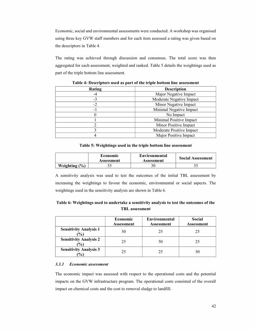
42

Economic, social and environmental assessments were conducted. A workshop was organised

using three key GVW staff members and for each item assessed a rating was given based on

the descriptors in Table 4.

The rating was achieved through discussion and consensus. The total score was then

aggregated for each assessment, weighted and ranked. Table 5 details the weightings used as

part of the triple bottom line assessment.

Table 4: Descriptors used as part of the triple bottom line assessment

Rating Description -4 Major Negative Impact -3 Moderate Negative Impact -2 Minor Negative Impact -1 Minimal Negative Impact 0 No Impact 1 Minimal Positive Impact 2 Minor Positive Impact 3 Moderate Positive Impact 4 Major Positive Impact

Table 5: Weightings used in the triple bottom line assessment

Economic

Assessment Environmental

Assessment Social Assessment

Weighting (%) 35 30 35

A sensitivity analysis was used to test the outcomes of the initial TBL assessment by

increasing the weightings to favour the economic, environmental or social aspects. The

weightings used in the sensitivity analysis are shown in Table 6.

Table 6: Weightings used to undertake a sensitivity analysis to test the outcomes of the

TBL assessment

Economic Assessment

Environmental Assessment

Social Assessment

Sensitivity Analysis 1 (%)

50 25 25

Sensitivity Analysis 2 (%)

25 50 25

Sensitivity Analysis 3 (%)

25 25 50

3.3.1 Economic assessment

The economic impact was assessed with respect to the operational costs and the potential

impacts on the GVW infrastructure program. The operational costs consisted of the overall

impact on chemical costs and the cost to removal sludge to landfill.

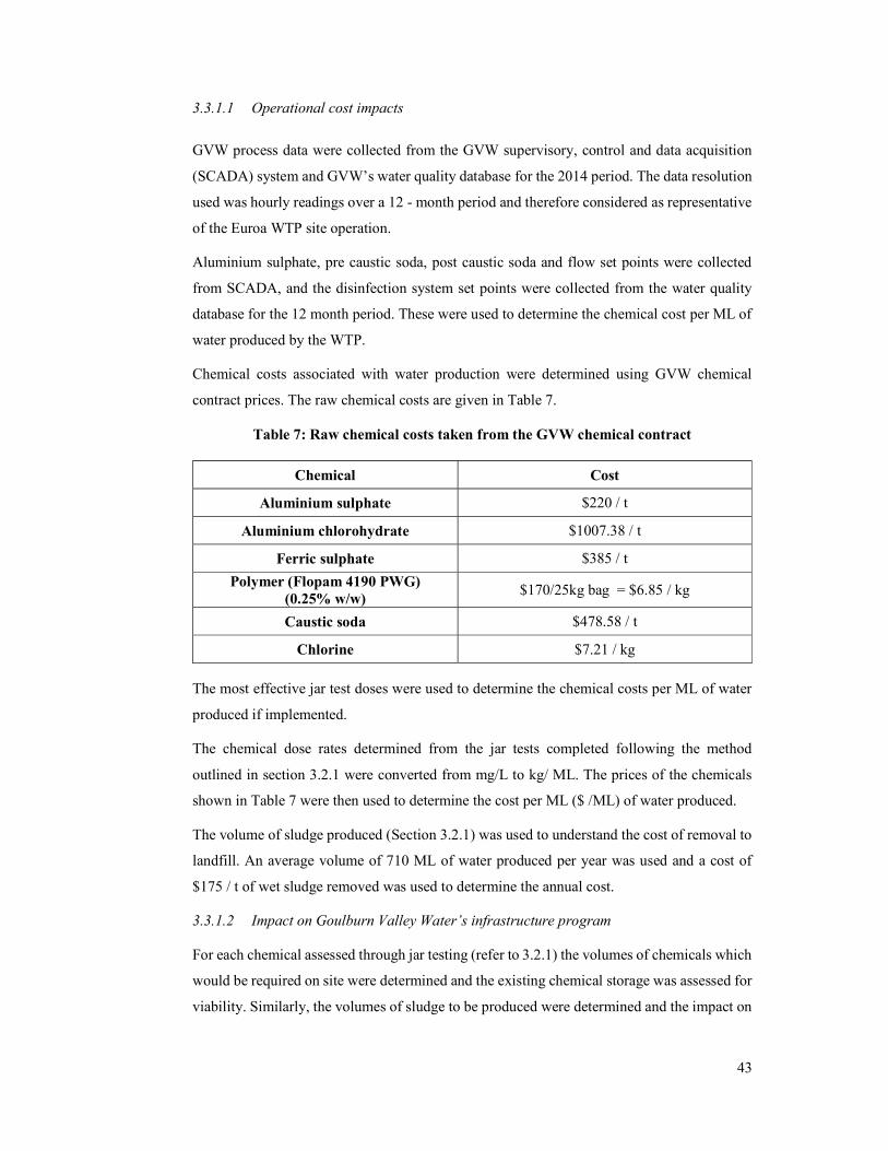
43

3.3.1.1 Operational cost impacts

GVW process data were collected from the GVW supervisory, control and data acquisition

(SCADA) system and GVW’s water quality database for the 2014 period. The data resolution

used was hourly readings over a 12 - month period and therefore considered as representative

of the Euroa WTP site operation.

Aluminium sulphate, pre caustic soda, post caustic soda and flow set points were collected

from SCADA, and the disinfection system set points were collected from the water quality

database for the 12 month period. These were used to determine the chemical cost per ML of

water produced by the WTP.

Chemical costs associated with water production were determined using GVW chemical

contract prices. The raw chemical costs are given in Table 7.

Table 7: Raw chemical costs taken from the GVW chemical contract

Chemical Cost

Aluminium sulphate $220 / t

Aluminium chlorohydrate $1007.38 / t

Ferric sulphate $385 / t

Polymer (Flopam 4190 PWG) (0.25% w/w)

$170/25kg bag = $6.85 / kg

Caustic soda $478.58 / t

Chlorine $7.21 / kg

The most effective jar test doses were used to determine the chemical costs per ML of water

produced if implemented.

The chemical dose rates determined from the jar tests completed following the method

outlined in section 3.2.1 were converted from mg/L to kg/ ML. The prices of the chemicals

shown in Table 7 were then used to determine the cost per ML ($ /ML) of water produced.

The volume of sludge produced (Section 3.2.1) was used to understand the cost of removal to

landfill. An average volume of 710 ML of water produced per year was used and a cost of

$175 / t of wet sludge removed was used to determine the annual cost.

3.3.1.2 Impact on Goulburn Valley Water’s infrastructure program

For each chemical assessed through jar testing (refer to 3.2.1) the volumes of chemicals which

would be required on site were determined and the existing chemical storage was assessed for

viability. Similarly, the volumes of sludge to be produced were determined and the impact on

44

the existing sludge handling facility was assessed for suitability. From this an assessment was

made whether the existing infrastructure would require modification.

3.3.2 Environmental assessment

The environmental assessment consisted of analysing each coagulant for potential greenhouse

gas (GHG) emissions based on the volume of chemical to be delivered to site per year. Data

from Seo, et al., (2016) detailing the carbon dioxide (CO2) emissions per km driven was used

to determine the maximum volume of CO2 emitted for each chemical. This method was also

used based on the volume of sludge to be removed to landfill and the associated GHG

emissions.

Similarly for each coagulant the volume of sludge produced based on an annual treated water

production of 710 ML was determined and the potential impacts on disposal to landfill were

considered, including where beneficial reuse was applicable.

3.3.3 Social assessment

The social assessment took into account the impact that changes in taste and odour would have

on both the community and GVW employees, with particular consideration given to the

impact on the site operator.

Items considered when determining the impact on the site operator were exposure to chemical

hazards and the ease of site operation. The site operation considered jar testing requirements,

the operability of the clarifier and sludge management. For GVW employees change in the

level of work satisfaction was considered based on previous research looking into the

correlation between improved service levels to the community and staff pride using previous

work undertaken by Bulgarella, 2005.

Community aspects were determined using previous research into taste and odour impacts on

the community including work by Jardine, et al. (1999) and Sinclair, et al., (2005)

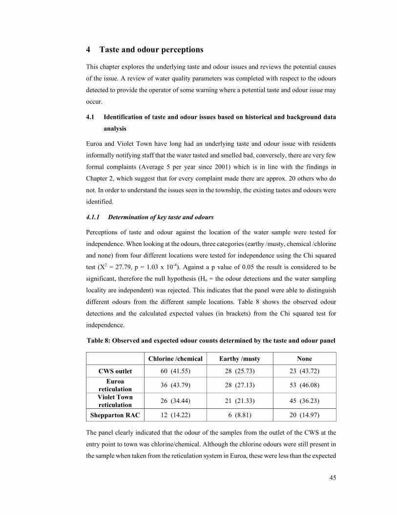
45

4 Taste and odour perceptions

This chapter explores the underlying taste and odour issues and reviews the potential causes

of the issue. A review of water quality parameters was completed with respect to the odours

detected to provide the operator of some warning where a potential taste and odour issue may

occur.

4.1 Identification of taste and odour issues based on historical and background data

analysis

Euroa and Violet Town have long had an underlying taste and odour issue with residents

informally notifying staff that the water tasted and smelled bad, conversely, there are very few

formal complaints (Average 5 per year since 2001) which is in line with the findings in

Chapter 2, which suggest that for every complaint made there are approx. 20 others who do

not. In order to understand the issues seen in the township, the existing tastes and odours were

identified.

4.1.1 Determination of key taste and odours

Perceptions of taste and odour against the location of the water sample were tested for

independence. When looking at the odours, three categories (earthy /musty, chemical /chlorine

and none) from four different locations were tested for independence using the Chi squared

test (Χ2 = 27.79, p = 1.03 x 10-4). Against a p value of 0.05 the result is considered to be

significant, therefore the null hypothesis (Ho = the odour detections and the water sampling

locality are independent) was rejected. This indicates that the panel were able to distinguish

different odours from the different sample locations. Table 8 shows the observed odour

detections and the calculated expected values (in brackets) from the Chi squared test for

independence.

Table 8: Observed and expected odour counts determined by the taste and odour panel

Chlorine /chemical Earthy /musty None

CWS outlet 60 (41.55) 28 (25.73) 23 (43.72)

Euroa reticulation

36 (43.79) 28 (27.13) 53 (46.08)

Violet Town reticulation

26 (34.44) 21 (21.33) 45 (36.23)

Shepparton RAC 12 (14.22) 6 (8.81) 20 (14.97)

The panel clearly indicated that the odour of the samples from the outlet of the CWS at the

entry point to town was chlorine/chemical. Although the chlorine odours were still present in

the sample when taken from the reticulation system in Euroa, these were less than the expected

46

values. Similar findings were found in the Violet Town samples. The panel determined that

earthy/musty odours were present in the CWS sample and also in the samples taken from the

reticulation systems in Euroa and Violet Town. All of these results are in line with the expected

values and it can be concluded that earthy /musty odours will often be present in Euroa water.

In the reticulation systems of both Euroa and Violet Town there were more ‘no odour’ detects

that the expected values, whereas the outlet of the CWS had fewer ‘no odour’ detects than

expected.

Based on the comparison of the observed and expected results it is apparent that the odours

being detected are changing as they move through the reticulation system. This is likely due

to interactions of chlorine and any dissolved matter in the water.

A similar process was used for taste detections. The Chi squared test for independence was

determined against the location (X2 = 10.07, p = 0.61), using a p value of 0.05, the null

hypothesis (Ho = the taste and sample locality are independent of each other) was accepted.

This means that the panel was unable to determine any difference in taste between locations.

The observed and expected results (in brackets) are shown in Table 9

Table 9: Observed and expected values from taste testing panels

Bitter None Salty Sour Sweet

CWS outlet 30 (26.41) 15 (15.96) 20 (22.64) 23 (23.51) 13 (12.48)

Euroa reticulation

27 (30.59) 22 (18.49) 25 (26.22) 26 (27.23) 17 (14.46)

Violet Town reticulation

20 (24.06) 11 (14.54) 26 (20.62) 26 (21.41) 9 (11.37)

Shepparton RAC

14 (9.94) 7 (6.01) 7 (8.52) 6 (8.84) 4 (4.70)

The data from Table 9 indicates that the panel were unable to distinguish between the tastes

of the water from different locations. However, the data in Table 8 shows that the panel were

able to discriminate odours from different locations. In general a person’s perceptions of

overall flavour is a combination of the odour and the taste of the water (Burlingame, et al.,

2017), it is likely that the panel’s perceptions are influenced mainly by the odour which

showed a greater sensitivity to location. Thus, it can be considered that the panel are more

accurately able to determine the odours from a particular location.

4.2 The Relationship of water quality parameters with respect to identified odours

From section 4.1, the panel determined the key odours at Euroa are earthy /musty and

chlorinous. From the literature, it is known that geosmin and MIB are key contributors to

earthy /musty odours within the source waters and chlorine has the ability to mask or oxidise

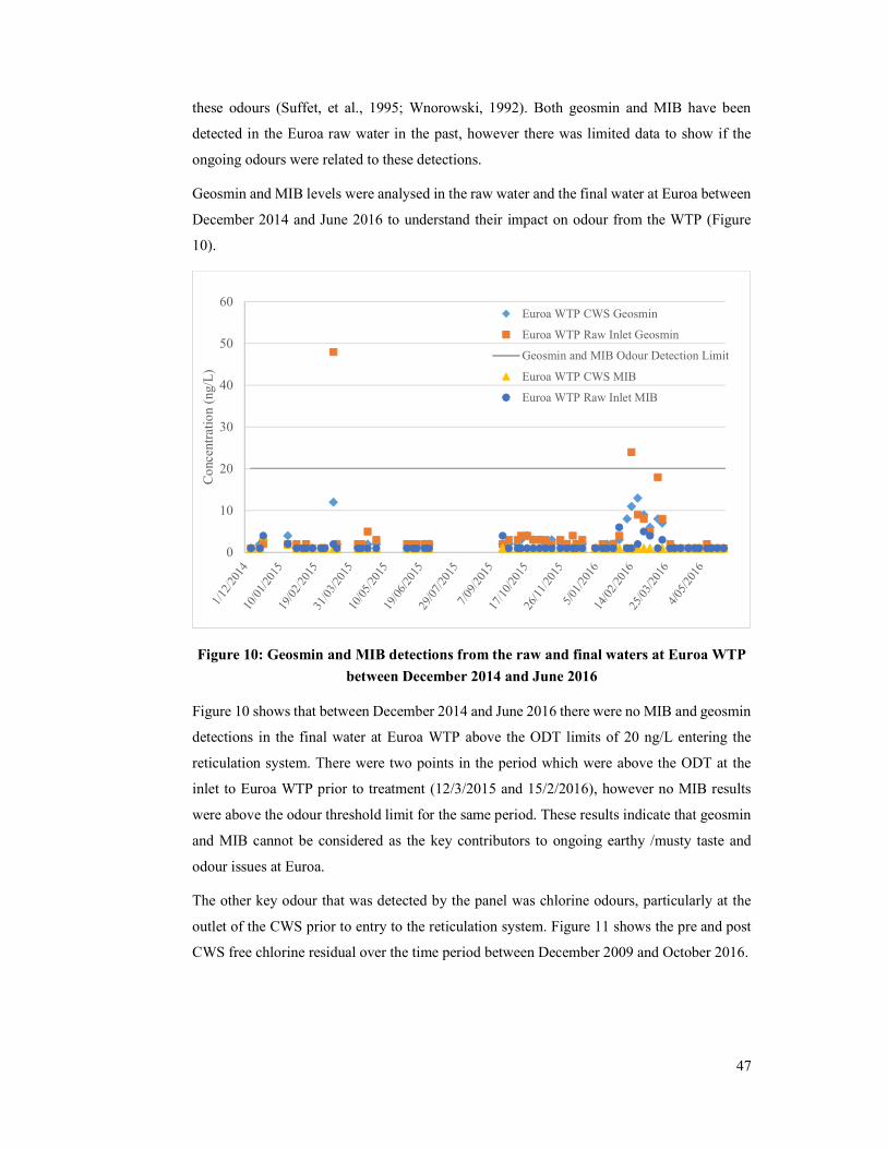
47

these odours (Suffet, et al., 1995; Wnorowski, 1992). Both geosmin and MIB have been

detected in the Euroa raw water in the past, however there was limited data to show if the

ongoing odours were related to these detections.

Geosmin and MIB levels were analysed in the raw water and the final water at Euroa between

December 2014 and June 2016 to understand their impact on odour from the WTP (Figure

10).

Figure 10: Geosmin and MIB detections from the raw and final waters at Euroa WTP

between December 2014 and June 2016

Figure 10 shows that between December 2014 and June 2016 there were no MIB and geosmin

detections in the final water at Euroa WTP above the ODT limits of 20 ng/L entering the

reticulation system. There were two points in the period which were above the ODT at the

inlet to Euroa WTP prior to treatment (12/3/2015 and 15/2/2016), however no MIB results

were above the odour threshold limit for the same period. These results indicate that geosmin

and MIB cannot be considered as the key contributors to ongoing earthy /musty taste and

odour issues at Euroa.

The other key odour that was detected by the panel was chlorine odours, particularly at the

outlet of the CWS prior to entry to the reticulation system. Figure 11 shows the pre and post

CWS free chlorine residual over the time period between December 2009 and October 2016.

0

10

20

30

40

50

60

Con

cent

ratio

n (n

g/L

)

Euroa WTP CWS Geosmin

Euroa WTP Raw Inlet Geosmin

Geosmin and MIB Odour Detection Limit

Euroa WTP CWS MIB

Euroa WTP Raw Inlet MIB

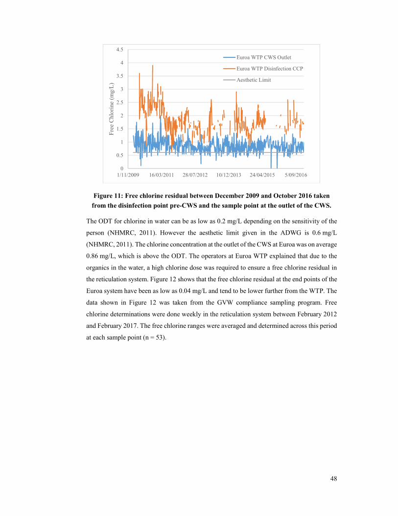
48

Figure 11: Free chlorine residual between December 2009 and October 2016 taken

from the disinfection point pre-CWS and the sample point at the outlet of the CWS.

The ODT for chlorine in water can be as low as 0.2 mg/L depending on the sensitivity of the

person (NHMRC, 2011). However the aesthetic limit given in the ADWG is 0.6 mg/L

(NHMRC, 2011). The chlorine concentration at the outlet of the CWS at Euroa was on average

0.86 mg/L, which is above the ODT. The operators at Euroa WTP explained that due to the

organics in the water, a high chlorine dose was required to ensure a free chlorine residual in

the reticulation system. Figure 12 shows that the free chlorine residual at the end points of the

Euroa system have been as low as 0.04 mg/L and tend to be lower further from the WTP. The

data shown in Figure 12 was taken from the GVW compliance sampling program. Free

chlorine determinations were done weekly in the reticulation system between February 2012

and February 2017. The free chlorine ranges were averaged and determined across this period

at each sample point (n = 53).

0

0.5

1

1.5

2

2.5

3

3.5

4

4.5

1/11/2009 16/03/2011 28/07/2012 10/12/2013 24/04/2015 5/09/2016

Fre

e C

hlor

ine

(mg/

L)

Euroa WTP CWS Outlet

Euroa WTP Disinfection CCP

Aesthetic Limit

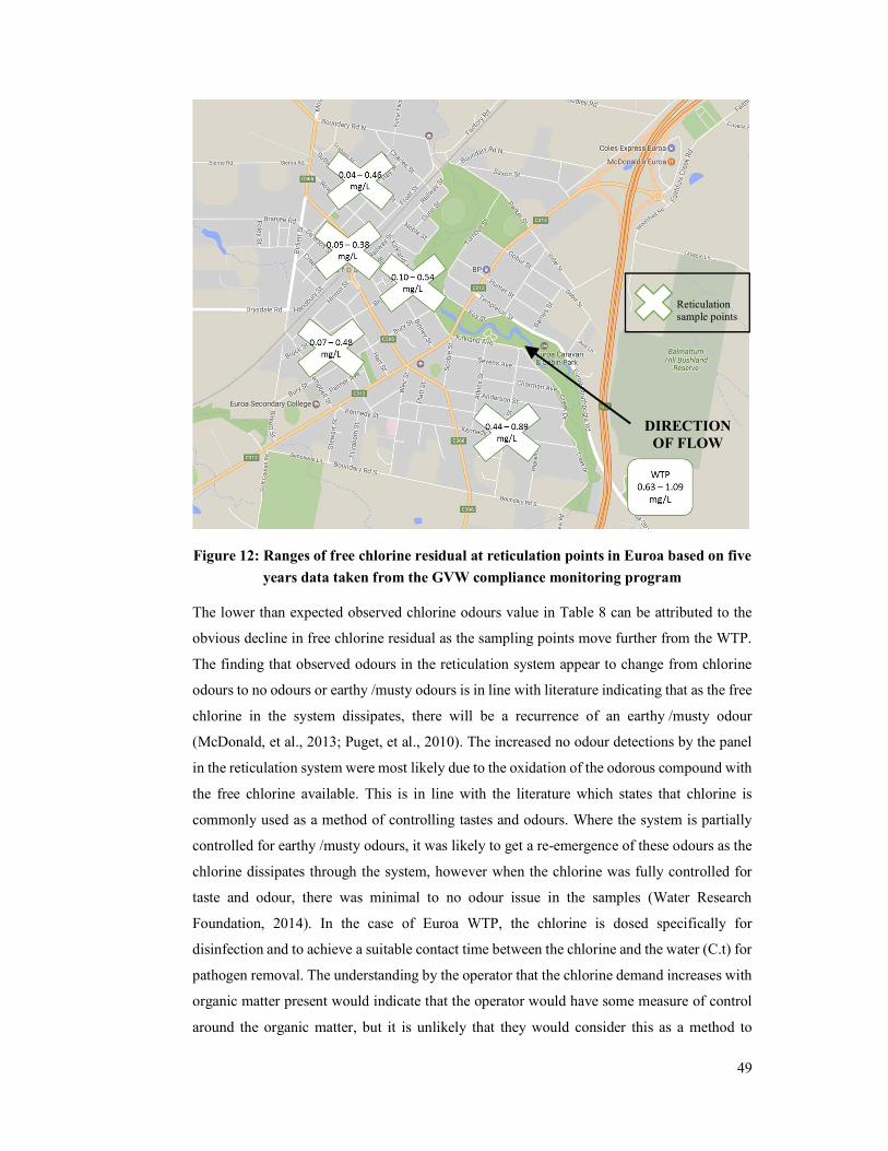
49

Figure 12: Ranges of free chlorine residual at reticulation points in Euroa based on five

years data taken from the GVW compliance monitoring program

The lower than expected observed chlorine odours value in Table 8 can be attributed to the

obvious decline in free chlorine residual as the sampling points move further from the WTP.

The finding that observed odours in the reticulation system appear to change from chlorine

odours to no odours or earthy /musty odours is in line with literature indicating that as the free

chlorine in the system dissipates, there will be a recurrence of an earthy /musty odour

(McDonald, et al., 2013; Puget, et al., 2010). The increased no odour detections by the panel

in the reticulation system were most likely due to the oxidation of the odorous compound with

the free chlorine available. This is in line with the literature which states that chlorine is

commonly used as a method of controlling tastes and odours. Where the system is partially

controlled for earthy /musty odours, it was likely to get a re-emergence of these odours as the

chlorine dissipates through the system, however when the chlorine was fully controlled for

taste and odour, there was minimal to no odour issue in the samples (Water Research

Foundation, 2014). In the case of Euroa WTP, the chlorine is dosed specifically for

disinfection and to achieve a suitable contact time between the chlorine and the water (C.t) for

pathogen removal. The understanding by the operator that the chlorine demand increases with

organic matter present would indicate that the operator would have some measure of control

around the organic matter, but it is unlikely that they would consider this as a method to

Reticulation sample points

DIRECTION OF FLOW

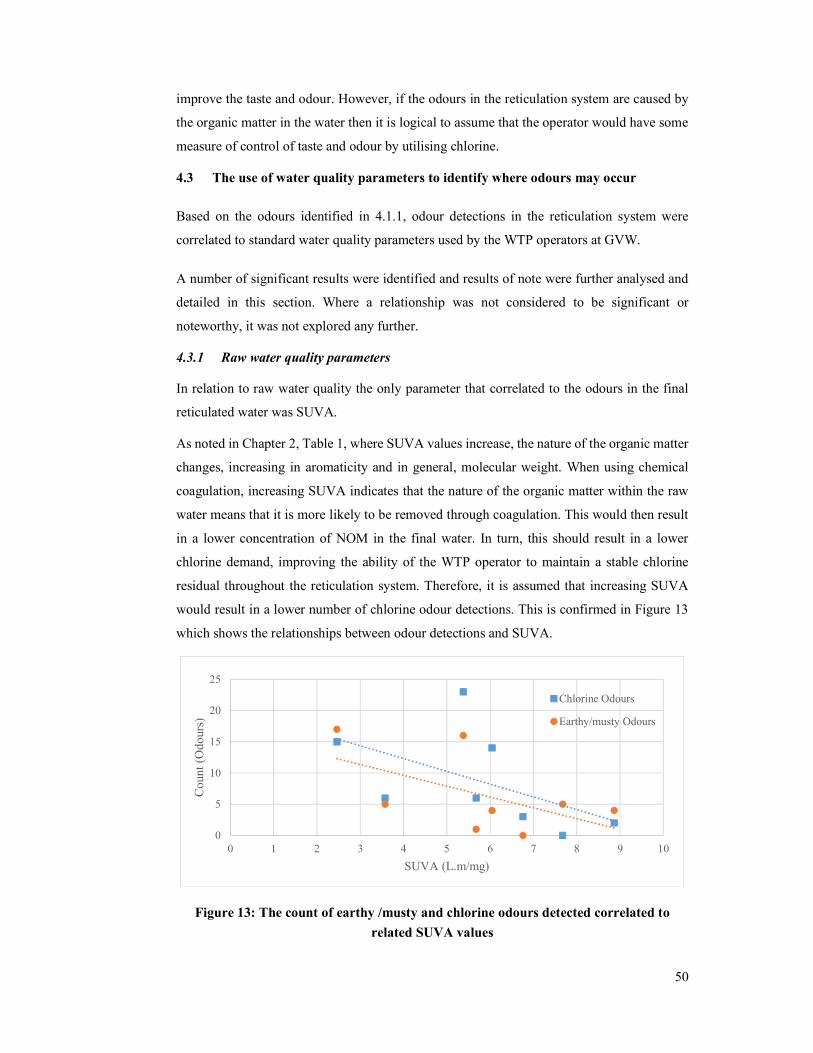
50

improve the taste and odour. However, if the odours in the reticulation system are caused by

the organic matter in the water then it is logical to assume that the operator would have some

measure of control of taste and odour by utilising chlorine.

4.3 The use of water quality parameters to identify where odours may occur

Based on the odours identified in 4.1.1, odour detections in the reticulation system were

correlated to standard water quality parameters used by the WTP operators at GVW.

A number of significant results were identified and results of note were further analysed and

detailed in this section. Where a relationship was not considered to be significant or

noteworthy, it was not explored any further.

4.3.1 Raw water quality parameters

In relation to raw water quality the only parameter that correlated to the odours in the final

reticulated water was SUVA.

As noted in Chapter 2, Table 1, where SUVA values increase, the nature of the organic matter

changes, increasing in aromaticity and in general, molecular weight. When using chemical

coagulation, increasing SUVA indicates that the nature of the organic matter within the raw

water means that it is more likely to be removed through coagulation. This would then result

in a lower concentration of NOM in the final water. In turn, this should result in a lower

chlorine demand, improving the ability of the WTP operator to maintain a stable chlorine

residual throughout the reticulation system. Therefore, it is assumed that increasing SUVA

would result in a lower number of chlorine odour detections. This is confirmed in Figure 13

which shows the relationships between odour detections and SUVA.

Figure 13: The count of earthy /musty and chlorine odours detected correlated to

related SUVA values

0

5

10

15

20

25

0 1 2 3 4 5 6 7 8 9 10

Cou

nt (

Odo

urs)

SUVA (L.m/mg)

Chlorine Odours

Earthy/musty Odours

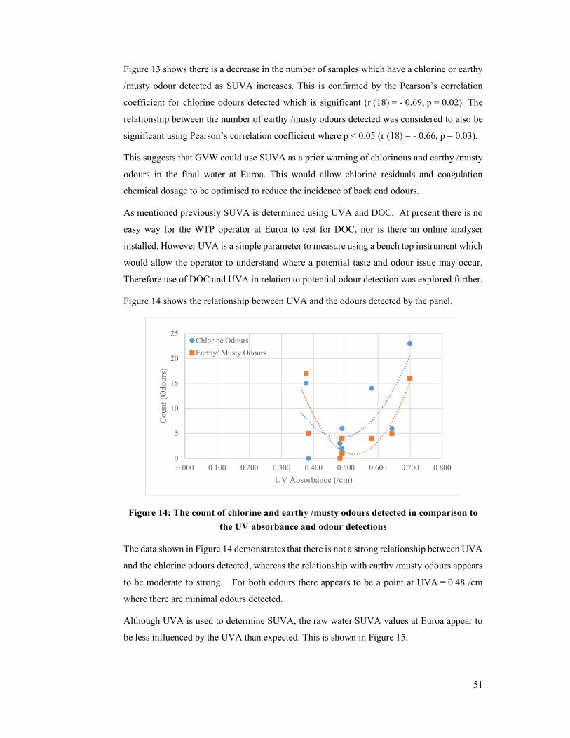
51

Figure 13 shows there is a decrease in the number of samples which have a chlorine or earthy

/musty odour detected as SUVA increases. This is confirmed by the Pearson’s correlation

coefficient for chlorine odours detected which is significant (r (18) = - 0.69, p = 0.02). The

relationship between the number of earthy /musty odours detected was considered to also be

significant using Pearson’s correlation coefficient where p < 0.05 (r (18) = - 0.66, p = 0.03).

This suggests that GVW could use SUVA as a prior warning of chlorinous and earthy /musty

odours in the final water at Euroa. This would allow chlorine residuals and coagulation

chemical dosage to be optimised to reduce the incidence of back end odours.

As mentioned previously SUVA is determined using UVA and DOC. At present there is no

easy way for the WTP operator at Euroa to test for DOC, nor is there an online analyser

installed. However UVA is a simple parameter to measure using a bench top instrument which

would allow the operator to understand where a potential taste and odour issue may occur.

Therefore use of DOC and UVA in relation to potential odour detection was explored further.

Figure 14 shows the relationship between UVA and the odours detected by the panel.

Figure 14: The count of chlorine and earthy /musty odours detected in comparison to

the UV absorbance and odour detections

The data shown in Figure 14 demonstrates that there is not a strong relationship between UVA

and the chlorine odours detected, whereas the relationship with earthy /musty odours appears

to be moderate to strong. For both odours there appears to be a point at UVA = 0.48 /cm

where there are minimal odours detected.

Although UVA is used to determine SUVA, the raw water SUVA values at Euroa appear to

be less influenced by the UVA than expected. This is shown in Figure 15.

0

5

10

15

20

25

0.000 0.100 0.200 0.300 0.400 0.500 0.600 0.700 0.800

Cou

nt (

Odo

urs)

UV Absorbance (/cm)

Chlorine Odours

Earthy/ Musty Odours

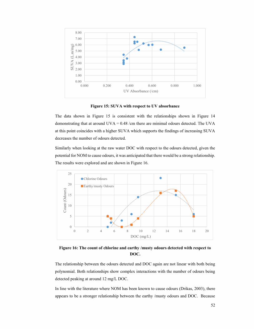
52

Figure 15: SUVA with respect to UV absorbance

The data shown in Figure 15 is consistent with the relationships shown in Figure 14

demonstrating that at around UVA = 0.48 /cm there are minimal odours detected. The UVA

at this point coincides with a higher SUVA which supports the findings of increasing SUVA

decreases the number of odours detected.

Similarly when looking at the raw water DOC with respect to the odours detected, given the

potential for NOM to cause odours, it was anticipated that there would be a strong relationship.

The results were explored and are shown in Figure 16.

Figure 16: The count of chlorine and earthy /musty odours detected with respect to

DOC.

The relationship between the odours detected and DOC again are not linear with both being

polynomial. Both relationships show complex interactions with the number of odours being

detected peaking at around 12 mg/L DOC.

In line with the literature where NOM has been known to cause odours (Drikas, 2003), there

appears to be a stronger relationship between the earthy /musty odours and DOC. Because

0.00

1.00

2.00

3.00

4.00

5.00

6.00

7.00

8.00

0.000 0.200 0.400 0.600 0.800 1.000

SU

VA

(L

.m/m

g)

UV Absorbance (/cm)

0

5

10

15

20

25

0 2 4 6 8 10 12 14 16 18 20

Cou

nt (

Odo

urs)

DOC (mg/L)

Chlorine Odours

Earthy/musty Odours

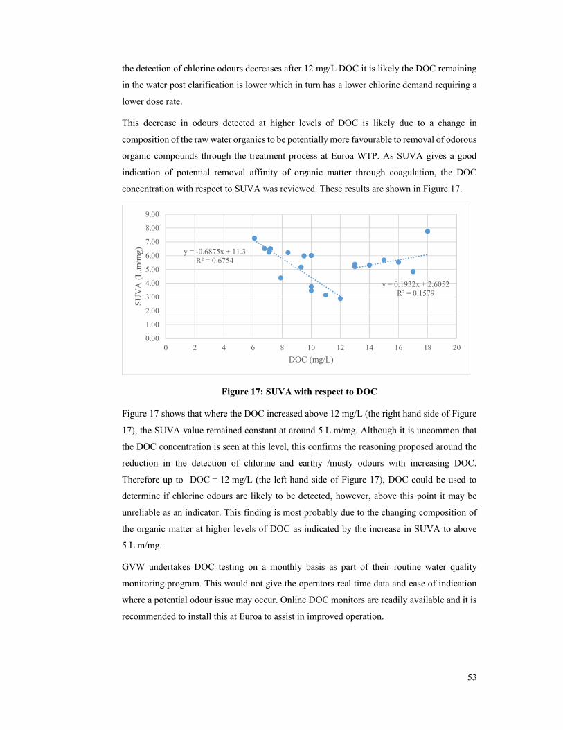
53

the detection of chlorine odours decreases after 12 mg/L DOC it is likely the DOC remaining

in the water post clarification is lower which in turn has a lower chlorine demand requiring a

lower dose rate.

This decrease in odours detected at higher levels of DOC is likely due to a change in

composition of the raw water organics to be potentially more favourable to removal of odorous

organic compounds through the treatment process at Euroa WTP. As SUVA gives a good

indication of potential removal affinity of organic matter through coagulation, the DOC

concentration with respect to SUVA was reviewed. These results are shown in Figure 17.

Figure 17: SUVA with respect to DOC

Figure 17 shows that where the DOC increased above 12 mg/L (the right hand side of Figure

17), the SUVA value remained constant at around 5 L.m/mg. Although it is uncommon that

the DOC concentration is seen at this level, this confirms the reasoning proposed around the

reduction in the detection of chlorine and earthy /musty odours with increasing DOC.

Therefore up to DOC = 12 mg/L (the left hand side of Figure 17), DOC could be used to

determine if chlorine odours are likely to be detected, however, above this point it may be

unreliable as an indicator. This finding is most probably due to the changing composition of

the organic matter at higher levels of DOC as indicated by the increase in SUVA to above

5 L.m/mg.

GVW undertakes DOC testing on a monthly basis as part of their routine water quality

monitoring program. This would not give the operators real time data and ease of indication

where a potential odour issue may occur. Online DOC monitors are readily available and it is

recommended to install this at Euroa to assist in improved operation.

y = -0.6875x + 11.3R² = 0.6754

y = 0.1932x + 2.6052R² = 0.1579

0.00

1.00

2.00

3.00

4.00

5.00

6.00

7.00

8.00

9.00

0 2 4 6 8 10 12 14 16 18 20

SUV

A (

L.m

/mg)

DOC (mg/L)

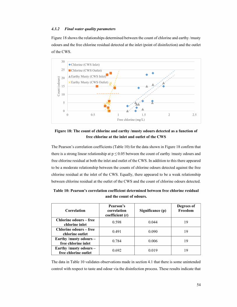
54

4.3.2 Final water quality parameters

Figure 18 shows the relationships determined between the count of chlorine and earthy /musty

odours and the free chlorine residual detected at the inlet (point of disinfection) and the outlet

of the CWS.

Figure 18: The count of chlorine and earthy /musty odours detected as a function of

free chlorine at the inlet and outlet of the CWS

The Pearson’s correlation coefficients (Table 10) for the data shown in Figure 18 confirm that

there is a strong linear relationship at p ≤ 0.05 between the count of earthy /musty odours and

free chlorine residual at both the inlet and outlet of the CWS. In addition to this there appeared

to be a moderate relationship between the counts of chlorine odours detected against the free

chlorine residual at the inlet of the CWS. Equally, there appeared to be a weak relationship

between chlorine residual at the outlet of the CWS and the count of chlorine odours detected.

Table 10: Pearson’s correlation coefficient determined between free chlorine residual

and the count of odours.

Correlation Pearson’s

correlation coefficient (r)

Significance (p) Degrees of Freedom

Chlorine odours – free chlorine inlet

0.598 0.044 19

Chlorine odours – free chlorine outlet

0.491 0.090 19

Earthy /musty odours – free chlorine inlet

0.784 0.006 19

Earthy /musty odours – free chlorine outlet

0.692 0.019 19

The data in Table 10 validates observations made in section 4.1 that there is some unintended

control with respect to taste and odour via the disinfection process. These results indicate that

0

5

10

15

20

25

30

0 0.5 1 1.5 2 2.5

Cou

nt (

odou

rs)

Free chlorine (mg/L)

Chlorine (CWS Inlet)

Chlorine (CWS Outlet)

Earthy Musty (CWS Inlet)

Earthy Musty (CWS Outlet)

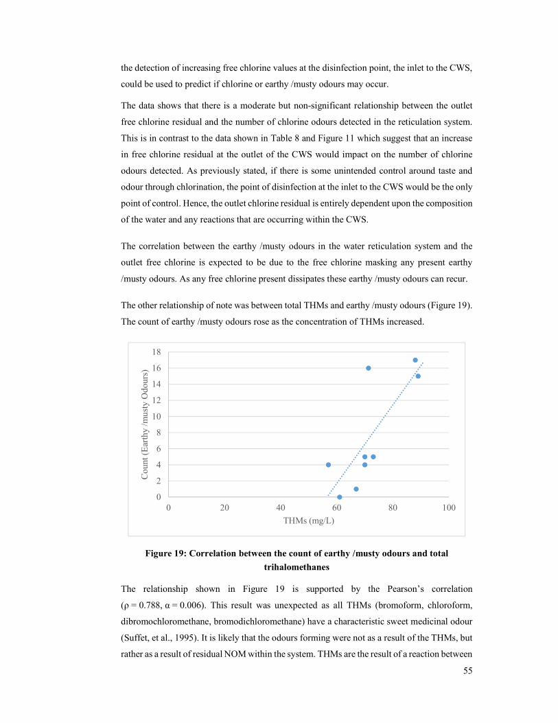
55

the detection of increasing free chlorine values at the disinfection point, the inlet to the CWS,

could be used to predict if chlorine or earthy /musty odours may occur.

The data shows that there is a moderate but non-significant relationship between the outlet

free chlorine residual and the number of chlorine odours detected in the reticulation system.

This is in contrast to the data shown in Table 8 and Figure 11 which suggest that an increase

in free chlorine residual at the outlet of the CWS would impact on the number of chlorine

odours detected. As previously stated, if there is some unintended control around taste and

odour through chlorination, the point of disinfection at the inlet to the CWS would be the only

point of control. Hence, the outlet chlorine residual is entirely dependent upon the composition

of the water and any reactions that are occurring within the CWS.

The correlation between the earthy /musty odours in the water reticulation system and the

outlet free chlorine is expected to be due to the free chlorine masking any present earthy

/musty odours. As any free chlorine present dissipates these earthy /musty odours can recur.

The other relationship of note was between total THMs and earthy /musty odours (Figure 19).

The count of earthy /musty odours rose as the concentration of THMs increased.

Figure 19: Correlation between the count of earthy /musty odours and total

trihalomethanes

The relationship shown in Figure 19 is supported by the Pearson’s correlation

(ρ = 0.788, α = 0.006). This result was unexpected as all THMs (bromoform, chloroform,

dibromochloromethane, bromodichloromethane) have a characteristic sweet medicinal odour

(Suffet, et al., 1995). It is likely that the odours forming were not as a result of the THMs, but

rather as a result of residual NOM within the system. THMs are the result of a reaction between

0

2

4

6

8

10

12

14

16

18

0 20 40 60 80 100

Cou

nt (

Ear

thy

/mus

ty O

dour

s)

THMs (mg/L)

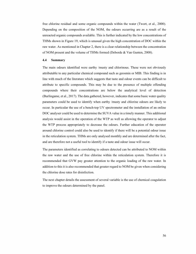
56

free chlorine residual and some organic compounds within the water (Twort, et al., 2000).

Depending on the composition of the NOM, the odours occurring are as a result of the

unreacted organic compounds available. This is further indicated by the low concentrations of

THMs shown in Figure 19, which is unusual given the high concentration of DOC within the

raw water. As mentioned in Chapter 2, there is a clear relationship between the concentration

of NOM present and the volume of THMs formed (Deborde & Van Gunten, 2008).

4.4 Summary

The main odours identified were earthy /musty and chlorinous. These were not obviously

attributable to any particular chemical compound such as geosmin or MIB. This finding is in

line with much of the literature which suggests that taste and odour events can be difficult to

attribute to specific compounds. This may be due to the presence of multiple offending

compounds where their concentrations are below the analytical level of detection

(Burlingame, et al., 2017). The data gathered, however, indicates that some basic water quality

parameters could be used to identify when earthy /musty and chlorine odours are likely to

occur. In particular the use of a bench-top UV spectrometer and the installation of an online

DOC analyser could be used to determine the SUVA value in a timely manner. This additional

analysis would assist in the operation of the WTP as well as allowing the operator to adjust

the WTP process appropriately to decrease the odours. Further education of the operator

around chlorine control could also be used to identify if there will be a potential odour issue

in the reticulation system. THMs are only analysed monthly and are determined after the fact,

and are therefore not a useful tool to identify if a taste and odour issue will occur.

The parameters identified as correlating to odours detected can be attributed to NOM within

the raw water and the use of free chlorine within the reticulation system. Therefore it is

recommended that GVW pay greater attention to the organic loading of the raw water. In

addition to this it is also recommended that greater regard to NOM be given when considering

the chlorine dose rates for disinfection.

The next chapter details the assessment of several variable is the use of chemical coagulation

to improve the odours determined by the panel.

57

5 Chemical coagulation for odour improvement

The findings in Chapter 4.1 show that water quality parameters which indicate the presence

of NOM could be used to identify odours. As organic matter is traditionally removed through

chemical coagulation, optimisation of the coagulation process was undertaken to improve taste

and odours (Drikas, 2003). Additionally as ferric sulphate and ACH have been shown to be

more effective at removing organic matter through coagulation (Jarvis, et al., 2012), these

coagulants were trialled to understand their impact on taste and odours.

5.1 Raw water quality analysis

As many of the parameters that could be used to identify a taste and odour issue were

associated with the raw water (SUVA, UVA and DOC), further understanding of the raw water

was required to optimise the treatment process for taste and odour reduction. The use of these

parameters identified as potentially indicative of odour detections occurring were considered

in the optimisation.

As mentioned in Chapter 1, the catchment that feeds Euroa WTP is a combination of forested

and cleared agricultural land that is used for mixed rotational farming between sheep and

annual crops. Due to the historic practices associated with the operation of the storages,

Mountain Hut water tends to be a mixture of water from Waterhouse and Abbinga Reservoirs.

The contribution of each reservoir to the make-up of Mountain Hut can be dependent upon

weather (including rainfall and stream-flow), operator preference and treatability. Table 11

shows the key organic indicators for the three raw water storages at Euroa.

Table 11: Water quality parameters for Raw water inlet /Mountain Hut, Waterhouse

and Abbinga Reservoirs (n = 16)

Raw water inlet/ Mountain Hut

Reservoir

Waterhouse Reservoir

Abbinga Reservoir

Average Std Dev Average Std Dev Average Std Dev DOC (mg/L) 11.4 3.69 14.8 1.79 11.2 2.60 UVA (/cm) 0.49 0.15 0.64 0.05 0.45 0.12

SUVA (L.m/mg)

4.92 1.63 4.44 0.47 4.54 1.32

pH 7.73 0.37 8.32 0.56 8.31 0.28

Waterhouse Reservoir is heavily forested with the feeder streams drying up in periods of dry

weather. During wet weather, when these feeder streams are running, significant amounts of

vegetation are washed into the storage. According to Lin (1977) decaying vegetation is one of

the more frequent causes of tastes and odours in drinking water, with earthy /musty odours

being the main ones detected.

58

Anecdotally, when Waterhouse Reservoir water is being treated taste and odour complaints

occur within a couple of days. Unfortunately there is not enough operational data to cross

check this against customer complaints. This observation is contradictory to the water quality

parameters shown in Table 11 when considering the correlations determined in Chapter 4.3.

The higher SUVA value shown indicates there should be fewer odours detected in the

reticulation system. As the water from Waterhouse Reservoir is gravity fed to Mountain Hut

reservoir, this is likely to change the treatability of the water prior to entering the WTP, and

so influencing the odours seen following the change.

Abbinga Reservoir is situated entirely within private farmland which explains the lower DOC

and UVA levels as less organic matter finds its way into the water body. The SUVA levels for

all three storages indicate a similar treatability for each.

Fluorescence EEMs were completed on a sample from each of the Reservoirs to understand

the fluorescent NOM content. The FRI technique method (Chen et al., 2003) was used to

quantify the visible fluorescent organic matter in each of the raw water storages. The spectral

volumes were integrated under five EEMs regions (Table 12).

Table 12: EEMs regions used in the fluorescence regional integration technique (taken

from Chen, et al., (2003))

Region Description Excitation Emission I Aromatic Protein Group I 220 nm – 270 nm 280 nm – 330 nm II Aromatic Protein Group II 220 nm – 270 nm 330 nm – 380 nm III Fulvic Acid- Like substances 220 nm – 270 nm 380 nm – 550 nm IV Soluble microbial by-products 270 nm – 440 nm 280 nm – 380 nm V Humic Acid - Like substances 270 nm – 440 nm 380 nm – 550 nm

It should be noted that recent literature states that the regions given by Chen et al’s method

(2003) are not as clearly defined as initially thought, and that instead the regions tend to

contain mixtures of the humic and fulvic acid like substances (Liu, et al., 2011). However, for

the purposes of this study, the Chen et al. method using regional integration was considered

suitable.

The DOC, UVA and SUVA values for the three reservoir samples treated by EEMs are shown

in Table 13.

Table 13: The DOC, UVA and SUVA values associated with the raw water samples

treated to EEMs

DOC (mg/L) UVA (/cm) SUVA (L.m/mg) Mountain Hut Reservoir/

raw water inlet 7.3 0.59 7.6

Abbinga Reservoir 7.9 0.60 7.6 Waterhouse Reservoir 11.0 0.62 8.0

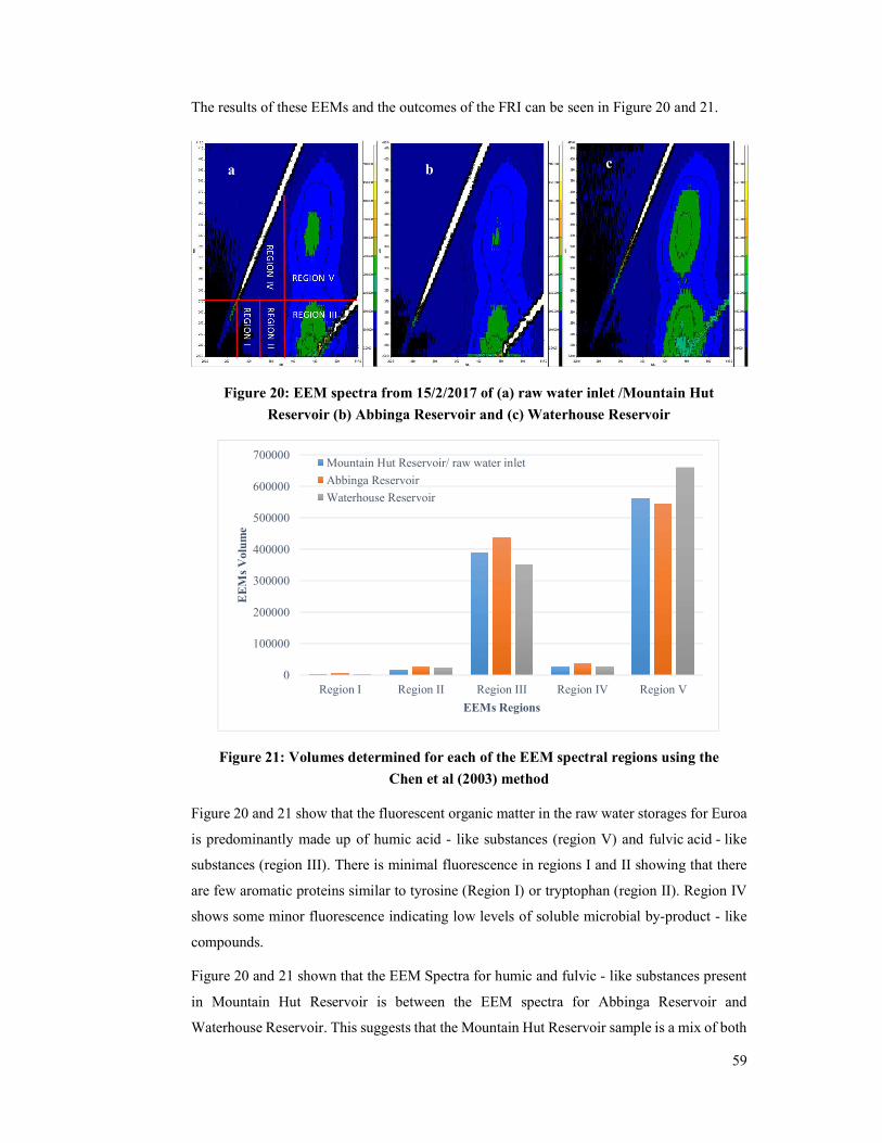
59

The results of these EEMs and the outcomes of the FRI can be seen in Figure 20 and 21.

Figure 20: EEM spectra from 15/2/2017 of (a) raw water inlet /Mountain Hut

Reservoir (b) Abbinga Reservoir and (c) Waterhouse Reservoir

Figure 21: Volumes determined for each of the EEM spectral regions using the

Chen et al (2003) method

Figure 20 and 21 show that the fluorescent organic matter in the raw water storages for Euroa

is predominantly made up of humic acid - like substances (region V) and fulvic acid - like

substances (region III). There is minimal fluorescence in regions I and II showing that there

are few aromatic proteins similar to tyrosine (Region I) or tryptophan (region II). Region IV

shows some minor fluorescence indicating low levels of soluble microbial by-product - like

compounds.

Figure 20 and 21 shown that the EEM Spectra for humic and fulvic - like substances present

in Mountain Hut Reservoir is between the EEM spectra for Abbinga Reservoir and

Waterhouse Reservoir. This suggests that the Mountain Hut Reservoir sample is a mix of both

0

100000

200000

300000

400000

500000

600000

700000

Region I Region II Region III Region IV Region V

EE

Ms

Vol

ume

EEMs Regions

Mountain Hut Reservoir/ raw water inlet

Abbinga Reservoir

Waterhouse Reservoir

a b c

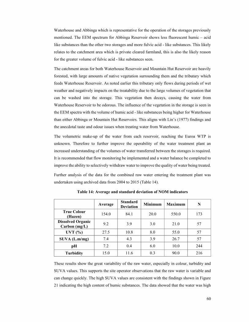
60

Waterhouse and Abbinga which is representative for the operation of the storages previously

mentioned. The EEM spectrum for Abbinga Reservoir shows less fluorescent humic – acid

like substances than the other two storages and more fulvic acid - like substances. This likely

relates to the catchment area which is private cleared farmland, this is also the likely reason

for the greater volume of fulvic acid - like substances seen.

The catchment areas for both Waterhouse Reservoir and Mountain Hut Reservoir are heavily

forested, with large amounts of native vegetation surrounding them and the tributary which

feeds Waterhouse Reservoir. As noted earlier this tributary only flows during periods of wet

weather and negatively impacts on the treatability due to the large volumes of vegetation that

can be washed into the storage. This vegetation then decays, causing the water from

Waterhouse Reservoir to be odorous. The influence of the vegetation in the storage is seen in

the EEM spectra with the volume of humic acid - like substances being higher for Waterhouse

than either Abbinga or Mountain Hut Reservoirs. This aligns with Lin’s (1977) findings and

the anecdotal taste and odour issues when treating water from Waterhouse.

The volumetric make-up of the water from each reservoir, reaching the Euroa WTP is

unknown. Therefore to further improve the operability of the water treatment plant an

increased understanding of the volumes of water transferred between the storages is required.

It is recommended that flow monitoring be implemented and a water balance be completed to

improve the ability to selectively withdraw water to improve the quality of water being treated.

Further analysis of the data for the combined raw water entering the treatment plant was

undertaken using archived data from 2004 to 2015 (Table 14).

Table 14: Average and standard deviation of NOM indicators

Average Standard Deviation

Minimum Maximum N

True Colour (Hazen)

154.0 84.1 20.0 550.0 173

Dissolved Organic Carbon (mg/L)

9.2 3.9 3.0 21.0 57

UVT (%) 27.5 10.8 8.0 55.0 57

SUVA (L.m/mg) 7.4 4.3 3.9 26.7 57

pH 7.2 0.4 6.0 10.0 244

Turbidity 15.0 11.6 0.3 90.0 216

These results show the great variability of the raw water, especially in colour, turbidity and

SUVA values. This supports the site operator observations that the raw water is variable and

can change quickly. The high SUVA values are consistent with the findings shown in Figure

21 indicating the high content of humic substances. The data showed that the water was high

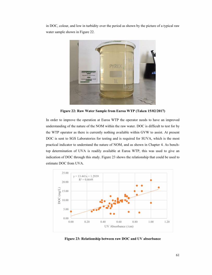
61

in DOC, colour, and low in turbidity over the period as shown by the picture of a typical raw

water sample shown in Figure 22.

Figure 22: Raw Water Sample from Euroa WTP (Taken 15/02/2017)

In order to improve the operation at Euroa WTP the operator needs to have an improved

understanding of the nature of the NOM within the raw water. DOC is difficult to test for by

the WTP operator as there is currently nothing available within GVW to assist. At present

DOC is sent to SGS Laboratories for testing and is required for SUVA, which is the most

practical indicator to understand the nature of NOM, and as shown in Chapter 4. As bench-

top determination of UVA is readily available at Euroa WTP, this was used to give an

indication of DOC through this study. Figure 23 shows the relationship that could be used to

estimate DOC from UVA.

Figure 23: Relationship between raw DOC and UV absorbance

y = 13.441x + 1.2939R² = 0.4649

0.00

5.00

10.00

15.00

20.00

25.00

0.00 0.20 0.40 0.60 0.80 1.00 1.20

DO

C (

mg/

L)

UV Absorbance (/cm)

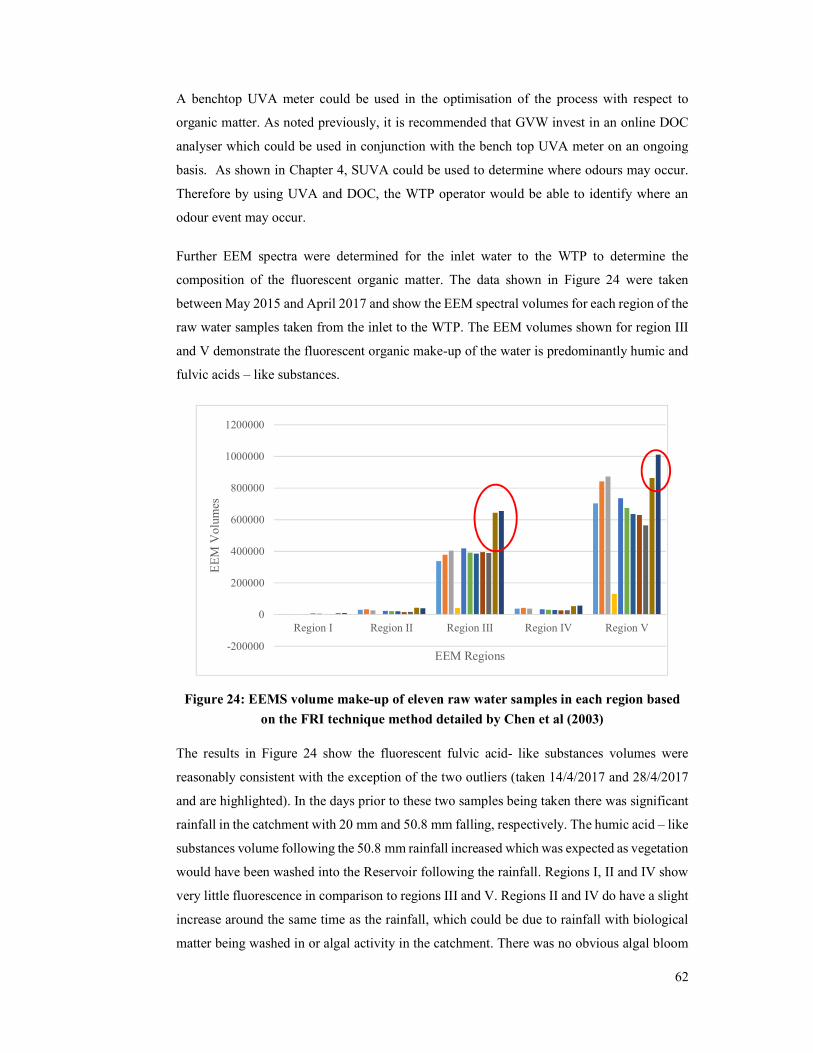
62

A benchtop UVA meter could be used in the optimisation of the process with respect to

organic matter. As noted previously, it is recommended that GVW invest in an online DOC

analyser which could be used in conjunction with the bench top UVA meter on an ongoing

basis. As shown in Chapter 4, SUVA could be used to determine where odours may occur.

Therefore by using UVA and DOC, the WTP operator would be able to identify where an

odour event may occur.

Further EEM spectra were determined for the inlet water to the WTP to determine the

composition of the fluorescent organic matter. The data shown in Figure 24 were taken

between May 2015 and April 2017 and show the EEM spectral volumes for each region of the

raw water samples taken from the inlet to the WTP. The EEM volumes shown for region III

and V demonstrate the fluorescent organic make-up of the water is predominantly humic and

fulvic acids – like substances.

Figure 24: EEMS volume make-up of eleven raw water samples in each region based

on the FRI technique method detailed by Chen et al (2003)

The results in Figure 24 show the fluorescent fulvic acid- like substances volumes were

reasonably consistent with the exception of the two outliers (taken 14/4/2017 and 28/4/2017

and are highlighted). In the days prior to these two samples being taken there was significant

rainfall in the catchment with 20 mm and 50.8 mm falling, respectively. The humic acid – like

substances volume following the 50.8 mm rainfall increased which was expected as vegetation

would have been washed into the Reservoir following the rainfall. Regions I, II and IV show

very little fluorescence in comparison to regions III and V. Regions II and IV do have a slight

increase around the same time as the rainfall, which could be due to rainfall with biological

matter being washed in or algal activity in the catchment. There was no obvious algal bloom

-200000

0

200000

400000

600000

800000

1000000

1200000

Region I Region II Region III Region IV Region V

EE

M V

olum

es

EEM Regions

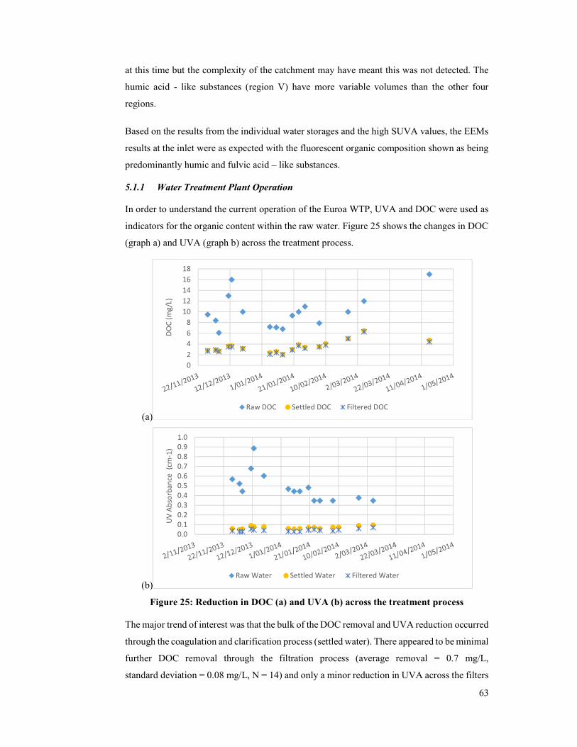
63

at this time but the complexity of the catchment may have meant this was not detected. The

humic acid - like substances (region V) have more variable volumes than the other four

regions.

Based on the results from the individual water storages and the high SUVA values, the EEMs

results at the inlet were as expected with the fluorescent organic composition shown as being

predominantly humic and fulvic acid – like substances.

5.1.1 Water Treatment Plant Operation

In order to understand the current operation of the Euroa WTP, UVA and DOC were used as

indicators for the organic content within the raw water. Figure 25 shows the changes in DOC

(graph a) and UVA (graph b) across the treatment process.

(a)

(b)

Figure 25: Reduction in DOC (a) and UVA (b) across the treatment process

The major trend of interest was that the bulk of the DOC removal and UVA reduction occurred

through the coagulation and clarification process (settled water). There appeared to be minimal

further DOC removal through the filtration process (average removal = 0.7 mg/L,

standard deviation = 0.08 mg/L, N = 14) and only a minor reduction in UVA across the filters

02468

1012141618

DO

C (m

g/L)

Raw DOC Settled DOC Filtered DOC

0.00.10.20.30.40.50.60.70.80.91.0

UV

Abso

rban

ce(c

m-1

)

Raw Water Settled Water Filtered Water

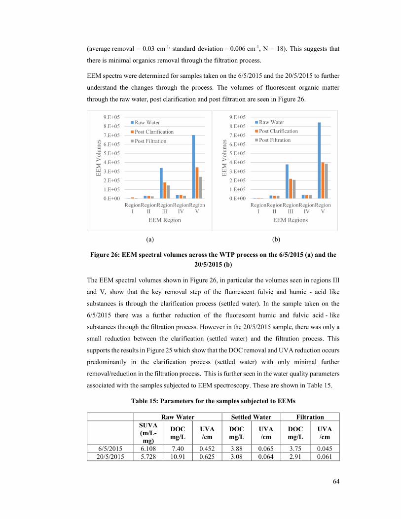
64

(average removal = 0.03 cm-1, standard deviation = 0.006 cm-1, N = 18). This suggests that

there is minimal organics removal through the filtration process.

EEM spectra were determined for samples taken on the 6/5/2015 and the 20/5/2015 to further

understand the changes through the process. The volumes of fluorescent organic matter

through the raw water, post clarification and post filtration are seen in Figure 26.

(a) (b)

Figure 26: EEM spectral volumes across the WTP process on the 6/5/2015 (a) and the

20/5/2015 (b)

The EEM spectral volumes shown in Figure 26, in particular the volumes seen in regions III

and V, show that the key removal step of the fluorescent fulvic and humic - acid like

substances is through the clarification process (settled water). In the sample taken on the

6/5/2015 there was a further reduction of the fluorescent humic and fulvic acid - like

substances through the filtration process. However in the 20/5/2015 sample, there was only a

small reduction between the clarification (settled water) and the filtration process. This

supports the results in Figure 25 which show that the DOC removal and UVA reduction occurs

predominantly in the clarification process (settled water) with only minimal further

removal/reduction in the filtration process. This is further seen in the water quality parameters

associated with the samples subjected to EEM spectroscopy. These are shown in Table 15.

Table 15: Parameters for the samples subjected to EEMs

Raw Water Settled Water Filtration

SUVA (m/L-mg)

DOC mg/L

UVA /cm

DOC mg/L

UVA /cm

DOC mg/L

UVA /cm

6/5/2015 6.108 7.40 0.452 3.88 0.065 3.75 0.045 20/5/2015 5.728 10.91 0.625 3.08 0.064 2.91 0.061

0.E+00

1.E+05

2.E+05

3.E+05

4.E+05

5.E+05

6.E+05

7.E+05

8.E+05

9.E+05

RegionI

RegionII

RegionIII

RegionIV

RegionV

EE

M V

olum

es

EEM Region

Raw Water

Post Clarification

Post Filtration

0.E+00

1.E+05

2.E+05

3.E+05

4.E+05

5.E+05

6.E+05

7.E+05

8.E+05

9.E+05

RegionI

RegionII

RegionIII

RegionIV

RegionV

EE

M V

olum

esEEM Regions

Raw Water

Post Clarification

Post Filtration

65

Based on this data it is clear that the main removal process for organics is coagulation with

little further removal occurring in the filtration process. Therefore, in order to improve the

removal rates of organics, the coagulation process was focussed on.

5.2 Comparison of coagulants

Coagulation with ferric sulphate and ACH was compared with aluminium sulphate, which is

currently used, for organics removal. UVA and DOC were used as measures of effectiveness

for organics removal. Jar testing was completed to mimic the existing plant conditions, with

odour testing performed to determine the improvements in odour. EEMs were undertaken to

understand the changes in fluorescent organic makeup and DOC and UVA removal.

5.2.1 Comparison of coagulant dose rates

This section reviews the outcomes of jar tests using all three coagulants and compares the

chemical dose rates. The results from the jar tests can be found in Appendix 2.

5.2.1.1 Aluminium sulphate jar tests

Historically turbidity and colour have been used as a basis for determining the aluminium

sulphate dose. Discussions with the operator indicated that there was an understanding of the

organics present but, this was not considered when the dose rate was set. Further investigation

into the historic dose rates showed that the dose set by the operator had a closer affinity to the

SUVA values of the raw water than the colour or turbidity. The correlation between colour

and the alum dose rate was low with low significance when using Pearson’s correlation

coefficient (r = 0.16, p = 0.32). Similarly, when reviewing the influence of turbidity on the

coagulant dose the correlation was low with low significance (r = 0.178, p=0.29).

This suggests that although there was no conscious consideration given to the organics, there

was some unintended influence on the dose rate setting. The Pearson’s correlation coefficient

between the aluminium sulphate dose rate and SUVA showed the relationship was considered

moderately high (r = 0.63, p = 0.02) which seems to confirm the operator unintentionally

using the organics as a basis to determine the dose rate.

GVW procedures recommend that with changing water quality the raw water should be jar

tested to determine the optimal dose. With the variation seen in the raw water at Euroa WTP

this can be considered as time consuming and where there are conflicting priorities, these may

not be completed. A multivariate regression was completed using the turbidity and UVT

results from eleven jar tests completed between May 2015 and November 2015 to develop an

algorithm to assist the operators during periods of variable water quality. This is shown in

Equation 4. This was validated further and compared to subsequent jar tests. These results are

shown in Figure 27.

66

= . − . − . Equation 4

The target pH at the WTP is set at 6.2 which requires pH correction using caustic soda. This

was also used as the target for the jar tests using aluminium sulphate. The dose rates for the

jar tests were based on the amount of alkalinity consumed by the aluminium sulphate (0.45

mg consumed as CaCO3) and the amount of alkalinity added by the caustic (1.25 mg added as

CaCO3) in line with the guidance in Murray & Mosse (2015). This relationship is shown in

equation 5.

= .

. Equation 5

Equation 4 was validated further and compared to the subsequent jar tests. These results are

presented in Figure 27 which shows the comparison between the jar tested aluminium sulphate

and caustic dose rates, the operator set dose rate and the estimated dose rate. The estimated

dose rates are based on Equations 4 and 5.

(a)

(b)

Figure 27: Comparison of aluminium sulphate dose rates (a) and caustic soda dose

rates (b)

020406080

100120140160

1 2 3 4 5 6 7 8 9 10 11 12 13 14 15 16Che

mic

al D

ose

Rat

e (m

g/L

)

Jar Test Number

Jar test dose rate Estimated dose rate WTP dose rate

0

10

20

30

40

50

60

1 2 3 4 5 6 7 8 9 10 11 12 13 14 15 16Che

mic

al D

ose

Rat

e (m

g/L

)

Jar Test Number

Jar test dose rate Estimated dose rate WTP dose rate

67

The variability seen between the WTP dose rates, the jar tested dose rates and the estimated

dose rates shown in Figure 27 demonstrates that the estimated dose rate from Equation 4

should be used as a guide only. The accuracy of this could be improved by adding more jar

test data into the regression used. These dose rates tended to be more consistent when

compared to the best dose rates from the jar tests. Similarly the estimated caustic dose rate

based on alkalinity was much higher than either the actual dose rate or the jar tested caustic

dose rate. The aluminium sulphate dose rate set by the operator was sometimes higher than

both the optimal jar tested dose and the estimated dose. This was expected due to the

operational practices around overdosing to combat changing raw water quality.

5.2.1.2 Ferric sulphate jar tests

Ferric sulphate has been shown to have greater DOC removal capacity than aluminium

sulphate and is normally used in waters with high organic loading (Matilainen, et al., 2010).

In general a lower dose rate is required for ferric sulphate than for aluminium sulphate,

however it has been known to form greater amounts of sludge and waste water (Twort, et al.,

2000). Figure 28 shows the optimal ferric sulphate doses from the jar tests which were

completed between August 2016 and April 2017.

(a)

(b)

Figure 28: Ferric sulphate (a) and caustic soda (b) jar tested dose rates

0

20

40

60

80

100

120

140

1 2 3 4 5 6 7 8 9

Che

mic

al D

ose

Rat

e (m

g/L

)

Sample Number

0

10

20

30

40

50

60

70

1 2 3 4 5 6 7 8 9

Che

mic

al D

ose

Rat

e (m

g/L

)

Sample Number

68

In the jar tested samples seen in Figure 28 the target pH for coagulation was pH 5 which is

within the optimal range (pH 4.8 – 6) for organics removal with ferric sulphate (Matilainen,

et al., 2010). Coagulation was conducted at a lower pH than the aluminium sulphate jar tests

(target pH = 6.1), which resulted in a lower caustic soda dose rate for pH correction compared

with using aluminium sulphate. The literature around coagulation suggests that DOC removal

should be between 29 % and 70 % using ferric sulphate at a lower pH (Matilainen, et al.,

2010).

5.2.1.3 Aluminium chlorohydrate jar tests

ACH was selected as a third option as it is used as an alternative to aluminium sulphate at

other GVW WTPs. It is considered to be more effective over a broader pH range which makes

it simpler to use than aluminium sulphate or ferric sulphate (Matilainen, et al., 2010). The

general operational rule of thumb is that the ACH dose is one third of the aluminium sulphate

dose rate which is due to the higher concentrations of Al2O3 present (23-25% and 7-9%,

respectively) which is the basis of floc formation (Murray and Mosse, 2015). The ACH dose

rates from jar tests completed between November 2015 and April 2017 are shown in Figure

29. No pH correction was required so caustic soda dose rates were not reviewed.

Figure 29: ACH jar tested dose rates.

The design of the clarifier at Euroa WTP requires a heavy floc blanket to be effective. The

sludge produced as a result of ACH coagulation was light in nature and slow to settle. The

existing site polymer which is used as a coagulation aid (Flopam 4190 PWG) was trialled to

increase the density of the sludge and allow for settlement. The polymer dose rates ranged

from 0.1 – 0.4 mg/L. Although this worked to some degree, the maximum recommended

polymer dose rate of 0.2 mg/L (Murray and Mosse, 2015) was exceeded and the sludge

produced was still slow to settle with floc still in suspension after 20 minutes. Although there

05

101520253035404550

1 2 3 4 5 6 7 8 9 10 11 12 13

Che

mic

al D

ose

Rat

e (m

g/L

)

Sample Number

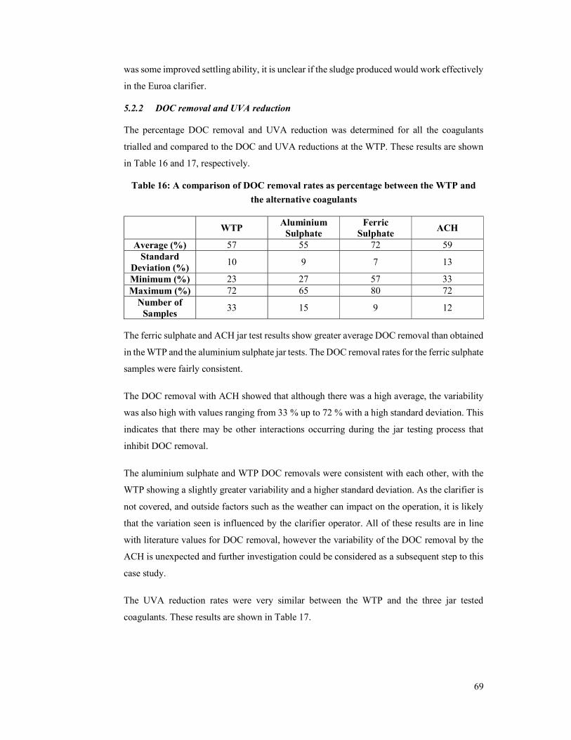
69

was some improved settling ability, it is unclear if the sludge produced would work effectively

in the Euroa clarifier.

5.2.2 DOC removal and UVA reduction

The percentage DOC removal and UVA reduction was determined for all the coagulants

trialled and compared to the DOC and UVA reductions at the WTP. These results are shown

in Table 16 and 17, respectively.

Table 16: A comparison of DOC removal rates as percentage between the WTP and

the alternative coagulants

WTP Aluminium

Sulphate Ferric

Sulphate ACH

Average (%) 57 55 72 59 Standard

Deviation (%) 10 9 7 13

Minimum (%) 23 27 57 33 Maximum (%) 72 65 80 72

Number of Samples

33 15 9 12

The ferric sulphate and ACH jar test results show greater average DOC removal than obtained

in the WTP and the aluminium sulphate jar tests. The DOC removal rates for the ferric sulphate

samples were fairly consistent.

The DOC removal with ACH showed that although there was a high average, the variability

was also high with values ranging from 33 % up to 72 % with a high standard deviation. This

indicates that there may be other interactions occurring during the jar testing process that

inhibit DOC removal.

The aluminium sulphate and WTP DOC removals were consistent with each other, with the

WTP showing a slightly greater variability and a higher standard deviation. As the clarifier is

not covered, and outside factors such as the weather can impact on the operation, it is likely

that the variation seen is influenced by the clarifier operator. All of these results are in line

with literature values for DOC removal, however the variability of the DOC removal by the

ACH is unexpected and further investigation could be considered as a subsequent step to this

case study.

The UVA reduction rates were very similar between the WTP and the three jar tested

coagulants. These results are shown in Table 17.

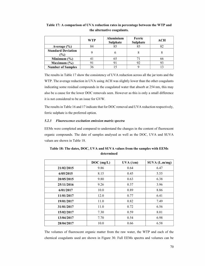
70

Table 17: A comparison of UVA reduction rates in percentage between the WTP and

the alternative coagulants.

WTP Aluminium

Sulphate Ferric

Sulphate ACH

Average (%) 84 85 85 82 Standard Deviation

(%) 9 6 8 8

Minimum (%) 41 65 71 66 Maximum (%) 91 91 92 93

Number of Samples 36 15 9 13

The results in Table 17 show the consistency of UVA reduction across all the jar tests and the

WTP. The average reduction in UVA using ACH was slightly lower than the other coagulants

indicating some residual compounds in the coagulated water that absorb at 254 nm, this may

also be a cause for the lower DOC removals seen. However as this is only a small difference

it is not considered to be an issue for GVW.

The results in Table 16 and 17 indicate that for DOC removal and UVA reduction respectively,

ferric sulphate is the preferred option.

5.2.3 Fluorescence excitation emission matrix spectra

EEMs were completed and compared to understand the changes in the content of fluorescent

organic compounds. The date of samples analysed as well as the DOC, UVA and SUVA

values are shown in Table 18.

Table 18: The dates, DOC, UVA and SUVA values from the samples with EEMs

determined

DOC (mg/L) UVA (/cm) SUVA (L.m/mg)

21/02/2015 9.86 0.64 6.47

6/05/2015 8.15 0.45 5.55

20/05/2015 9.80 0.63 6.38

25/11/2016 9.26 0.37 3.96

6/01/2017 10.0 0.89 8.86

11/01/2017 12.0 0.77 6.41

19/01/2017 11.0 0.82 7.49

31/01/2017 11.0 0.72 6.56

15/02/2017 7.30 0.59 8.01

13/04/2017 7.70 0.54 6.98

28/04/2017 10.0 0.66 6.58

The volumes of fluorescent organic matter from the raw water, the WTP and each of the

chemical coagulants used are shown in Figure 30. Full EEMs spectra and volumes can be

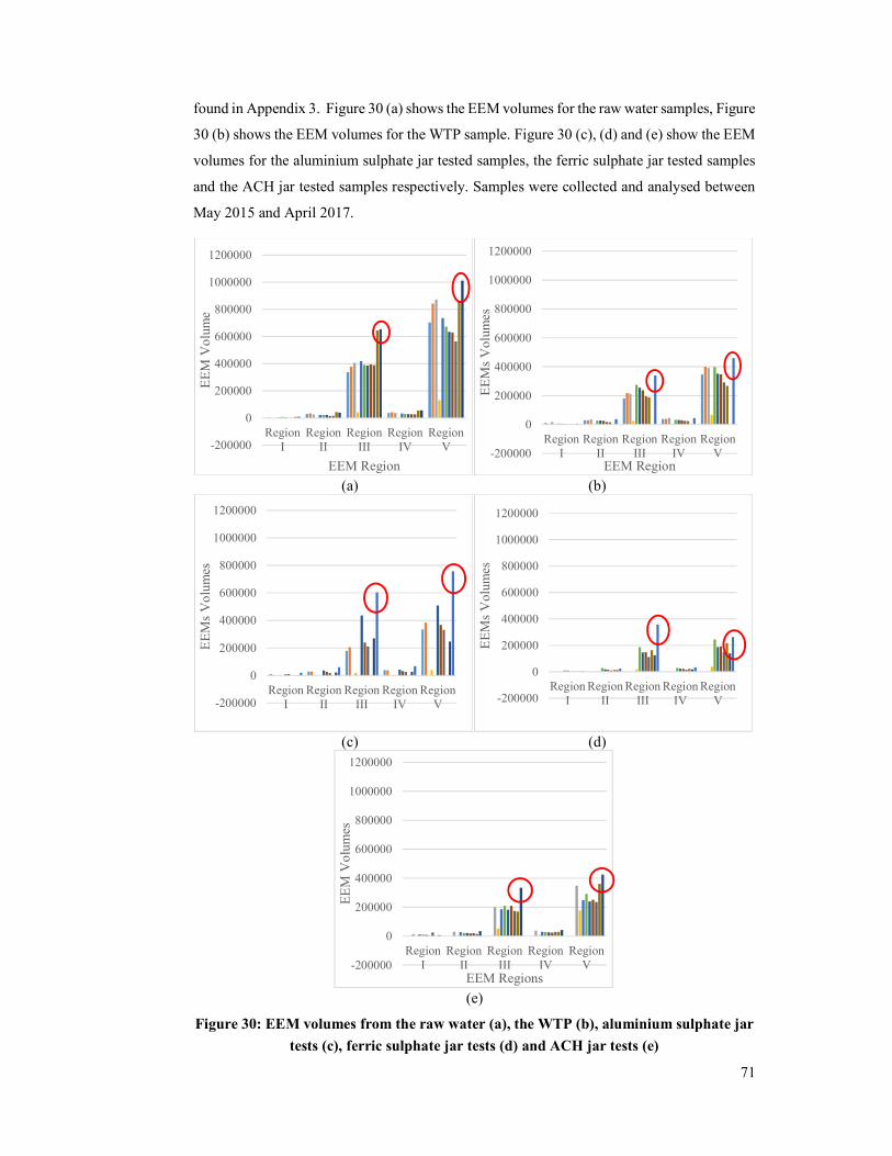
71

found in Appendix 3. Figure 30 (a) shows the EEM volumes for the raw water samples, Figure

30 (b) shows the EEM volumes for the WTP sample. Figure 30 (c), (d) and (e) show the EEM

volumes for the aluminium sulphate jar tested samples, the ferric sulphate jar tested samples

and the ACH jar tested samples respectively. Samples were collected and analysed between

May 2015 and April 2017.

(a) (b)

(c) (d)

(e)

Figure 30: EEM volumes from the raw water (a), the WTP (b), aluminium sulphate jar

tests (c), ferric sulphate jar tests (d) and ACH jar tests (e)

-200000

0

200000

400000

600000

800000

1000000

1200000

RegionI

RegionII

RegionIII

RegionIV

RegionV

EE

M V

olum

e

EEM Region-200000

0

200000

400000

600000

800000

1000000

1200000

RegionI

RegionII

RegionIII

RegionIV

RegionV

EE

Ms

Vol

umes

EEM Region

-200000

0

200000

400000

600000

800000

1000000

1200000

RegionI

RegionII

RegionIII

RegionIV

RegionV

EE

Ms

Vol

umes

-200000

0

200000

400000

600000

800000

1000000

1200000

RegionI

RegionII

RegionIII

RegionIV

RegionV

EE

Ms

Vol

umes

-200000

0

200000

400000

600000

800000

1000000

1200000

RegionI

RegionII

RegionIII

RegionIV

RegionV

EE

M V

olum

es

EEM Regions

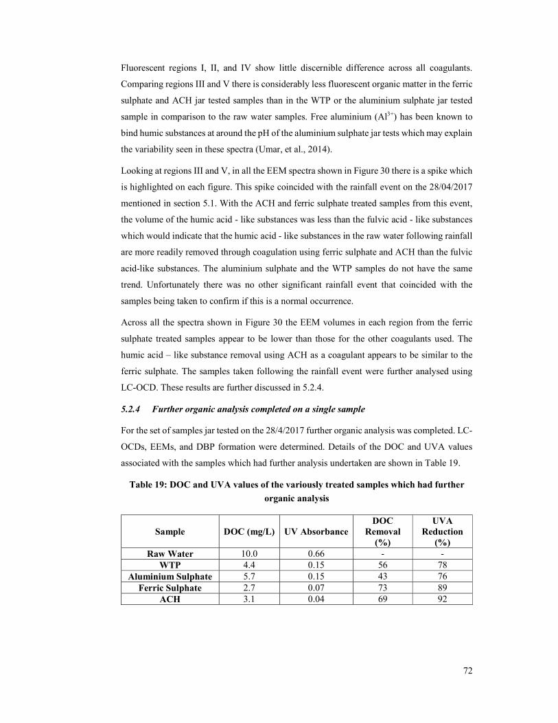
72

Fluorescent regions I, II, and IV show little discernible difference across all coagulants.

Comparing regions III and V there is considerably less fluorescent organic matter in the ferric

sulphate and ACH jar tested samples than in the WTP or the aluminium sulphate jar tested

sample in comparison to the raw water samples. Free aluminium (Al3+) has been known to

bind humic substances at around the pH of the aluminium sulphate jar tests which may explain

the variability seen in these spectra (Umar, et al., 2014).

Looking at regions III and V, in all the EEM spectra shown in Figure 30 there is a spike which

is highlighted on each figure. This spike coincided with the rainfall event on the 28/04/2017

mentioned in section 5.1. With the ACH and ferric sulphate treated samples from this event,

the volume of the humic acid - like substances was less than the fulvic acid - like substances

which would indicate that the humic acid - like substances in the raw water following rainfall

are more readily removed through coagulation using ferric sulphate and ACH than the fulvic

acid-like substances. The aluminium sulphate and the WTP samples do not have the same

trend. Unfortunately there was no other significant rainfall event that coincided with the

samples being taken to confirm if this is a normal occurrence.

Across all the spectra shown in Figure 30 the EEM volumes in each region from the ferric

sulphate treated samples appear to be lower than those for the other coagulants used. The

humic acid – like substance removal using ACH as a coagulant appears to be similar to the

ferric sulphate. The samples taken following the rainfall event were further analysed using

LC-OCD. These results are further discussed in 5.2.4.

5.2.4 Further organic analysis completed on a single sample

For the set of samples jar tested on the 28/4/2017 further organic analysis was completed. LC-

OCDs, EEMs, and DBP formation were determined. Details of the DOC and UVA values

associated with the samples which had further analysis undertaken are shown in Table 19.

Table 19: DOC and UVA values of the variously treated samples which had further

organic analysis

Sample DOC (mg/L) UV Absorbance DOC

Removal (%)

UVA Reduction

(%) Raw Water 10.0 0.66 - -

WTP 4.4 0.15 56 78 Aluminium Sulphate 5.7 0.15 43 76

Ferric Sulphate 2.7 0.07 73 89 ACH 3.1 0.04 69 92

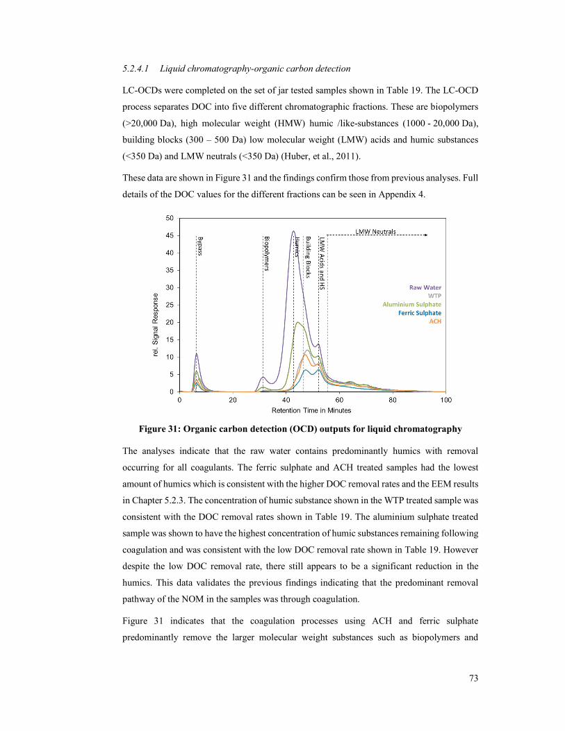
73

5.2.4.1 Liquid chromatography-organic carbon detection

LC-OCDs were completed on the set of jar tested samples shown in Table 19. The LC-OCD

process separates DOC into five different chromatographic fractions. These are biopolymers

(>20,000 Da), high molecular weight (HMW) humic /like-substances (1000 - 20,000 Da),

building blocks (300 – 500 Da) low molecular weight (LMW) acids and humic substances

(<350 Da) and LMW neutrals (<350 Da) (Huber, et al., 2011).

These data are shown in Figure 31 and the findings confirm those from previous analyses. Full

details of the DOC values for the different fractions can be seen in Appendix 4.

Figure 31: Organic carbon detection (OCD) outputs for liquid chromatography

The analyses indicate that the raw water contains predominantly humics with removal

occurring for all coagulants. The ferric sulphate and ACH treated samples had the lowest

amount of humics which is consistent with the higher DOC removal rates and the EEM results

in Chapter 5.2.3. The concentration of humic substance shown in the WTP treated sample was

consistent with the DOC removal rates shown in Table 19. The aluminium sulphate treated

sample was shown to have the highest concentration of humic substances remaining following

coagulation and was consistent with the low DOC removal rate shown in Table 19. However

despite the low DOC removal rate, there still appears to be a significant reduction in the

humics. This data validates the previous findings indicating that the predominant removal

pathway of the NOM in the samples was through coagulation.

Figure 31 indicates that the coagulation processes using ACH and ferric sulphate

predominantly remove the larger molecular weight substances such as biopolymers and

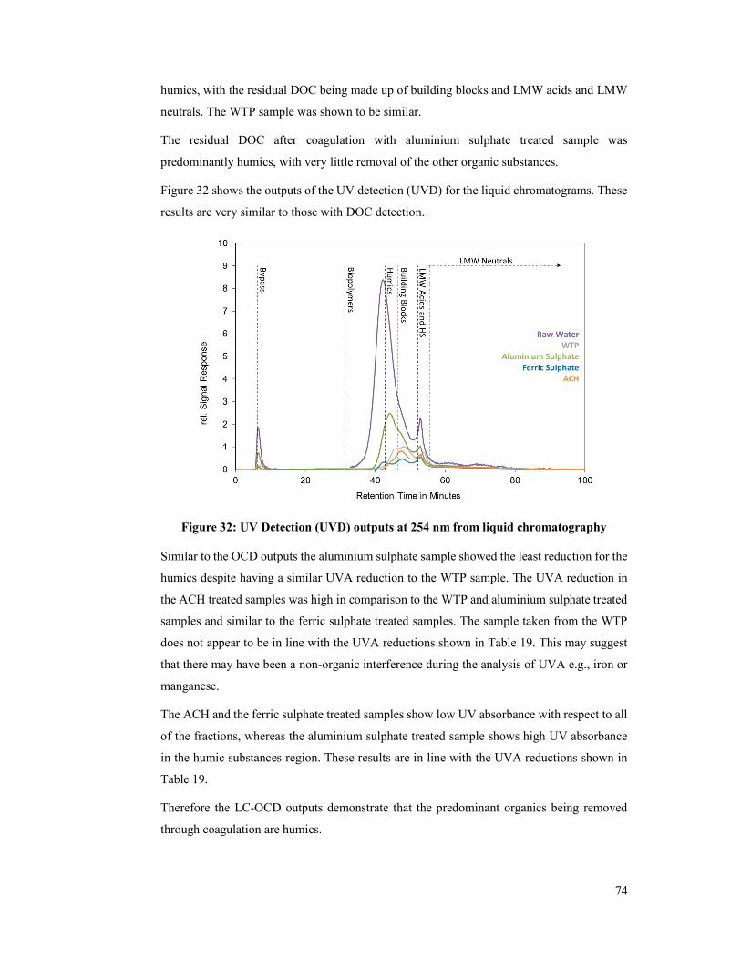
74

humics, with the residual DOC being made up of building blocks and LMW acids and LMW

neutrals. The WTP sample was shown to be similar.

The residual DOC after coagulation with aluminium sulphate treated sample was

predominantly humics, with very little removal of the other organic substances.

Figure 32 shows the outputs of the UV detection (UVD) for the liquid chromatograms. These

results are very similar to those with DOC detection.

Figure 32: UV Detection (UVD) outputs at 254 nm from liquid chromatography

Similar to the OCD outputs the aluminium sulphate sample showed the least reduction for the

humics despite having a similar UVA reduction to the WTP sample. The UVA reduction in

the ACH treated samples was high in comparison to the WTP and aluminium sulphate treated

samples and similar to the ferric sulphate treated samples. The sample taken from the WTP

does not appear to be in line with the UVA reductions shown in Table 19. This may suggest

that there may have been a non-organic interference during the analysis of UVA e.g., iron or

manganese.

The ACH and the ferric sulphate treated samples show low UV absorbance with respect to all

of the fractions, whereas the aluminium sulphate treated sample shows high UV absorbance

in the humic substances region. These results are in line with the UVA reductions shown in

Table 19.

Therefore the LC-OCD outputs demonstrate that the predominant organics being removed

through coagulation are humics.

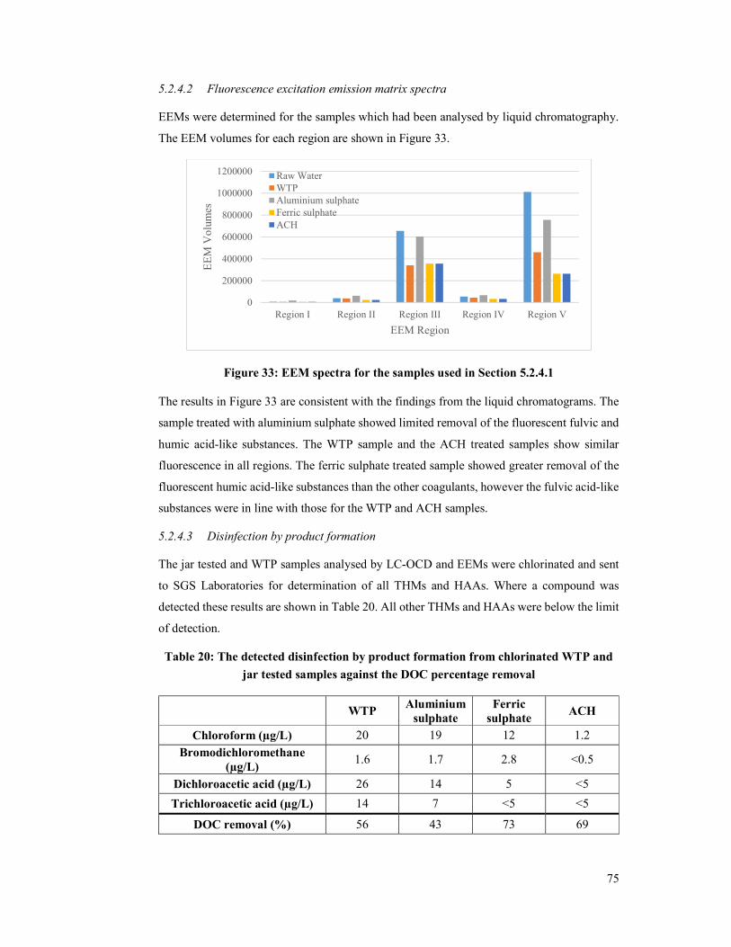
75

5.2.4.2 Fluorescence excitation emission matrix spectra

EEMs were determined for the samples which had been analysed by liquid chromatography.

The EEM volumes for each region are shown in Figure 33.

Figure 33: EEM spectra for the samples used in Section 5.2.4.1

The results in Figure 33 are consistent with the findings from the liquid chromatograms. The

sample treated with aluminium sulphate showed limited removal of the fluorescent fulvic and

humic acid-like substances. The WTP sample and the ACH treated samples show similar

fluorescence in all regions. The ferric sulphate treated sample showed greater removal of the

fluorescent humic acid-like substances than the other coagulants, however the fulvic acid-like

substances were in line with those for the WTP and ACH samples.

5.2.4.3 Disinfection by product formation

The jar tested and WTP samples analysed by LC-OCD and EEMs were chlorinated and sent

to SGS Laboratories for determination of all THMs and HAAs. Where a compound was

detected these results are shown in Table 20. All other THMs and HAAs were below the limit

of detection.

Table 20: The detected disinfection by product formation from chlorinated WTP and

jar tested samples against the DOC percentage removal

WTP Aluminium

sulphate Ferric

sulphate ACH

Chloroform (µg/L) 20 19 12 1.2

Bromodichloromethane (µg/L)

1.6 1.7 2.8 <0.5

Dichloroacetic acid (µg/L) 26 14 5 <5

Trichloroacetic acid (µg/L) 14 7 <5 <5

DOC removal (%) 56 43 73 69

0

200000

400000

600000

800000

1000000

1200000

Region I Region II Region III Region IV Region V

EE

M V

olum

es

EEM Region

Raw WaterWTPAluminium sulphateFerric sulphateACH

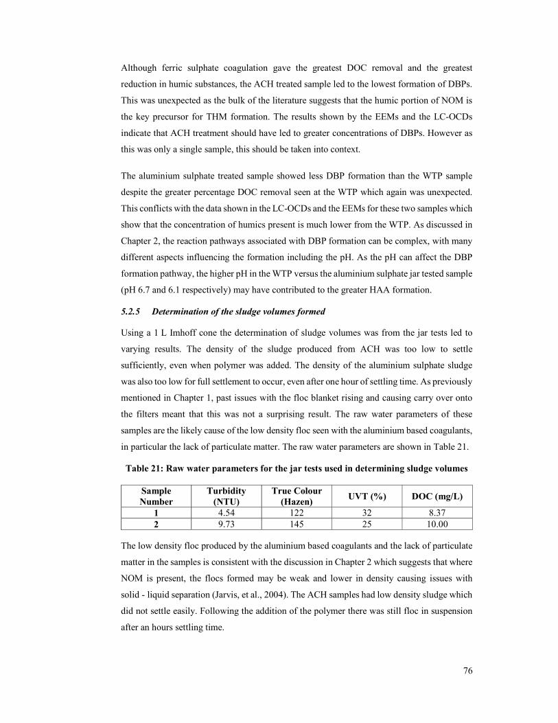
76

Although ferric sulphate coagulation gave the greatest DOC removal and the greatest

reduction in humic substances, the ACH treated sample led to the lowest formation of DBPs.

This was unexpected as the bulk of the literature suggests that the humic portion of NOM is

the key precursor for THM formation. The results shown by the EEMs and the LC-OCDs

indicate that ACH treatment should have led to greater concentrations of DBPs. However as

this was only a single sample, this should be taken into context.

The aluminium sulphate treated sample showed less DBP formation than the WTP sample

despite the greater percentage DOC removal seen at the WTP which again was unexpected.

This conflicts with the data shown in the LC-OCDs and the EEMs for these two samples which

show that the concentration of humics present is much lower from the WTP. As discussed in

Chapter 2, the reaction pathways associated with DBP formation can be complex, with many

different aspects influencing the formation including the pH. As the pH can affect the DBP

formation pathway, the higher pH in the WTP versus the aluminium sulphate jar tested sample

(pH 6.7 and 6.1 respectively) may have contributed to the greater HAA formation.

5.2.5 Determination of the sludge volumes formed

Using a 1 L Imhoff cone the determination of sludge volumes was from the jar tests led to

varying results. The density of the sludge produced from ACH was too low to settle

sufficiently, even when polymer was added. The density of the aluminium sulphate sludge

was also too low for full settlement to occur, even after one hour of settling time. As previously

mentioned in Chapter 1, past issues with the floc blanket rising and causing carry over onto

the filters meant that this was not a surprising result. The raw water parameters of these

samples are the likely cause of the low density floc seen with the aluminium based coagulants,

in particular the lack of particulate matter. The raw water parameters are shown in Table 21.

Table 21: Raw water parameters for the jar tests used in determining sludge volumes

Sample Number

Turbidity (NTU)

True Colour (Hazen)

UVT (%) DOC (mg/L)

1 4.54 122 32 8.37 2 9.73 145 25 10.00

The low density floc produced by the aluminium based coagulants and the lack of particulate

matter in the samples is consistent with the discussion in Chapter 2 which suggests that where

NOM is present, the flocs formed may be weak and lower in density causing issues with

solid - liquid separation (Jarvis, et al., 2004). The ACH samples had low density sludge which

did not settle easily. Following the addition of the polymer there was still floc in suspension

after an hours settling time.

77

The ferric sulphate floc, on the other hand, settled quickly and was dense and easy to measure,

as stated in Chapter 2, the density of the floc formed can be impacted on by factors such as

pH, in the case of the ferric sulphate treated samples, coagulation occurred at pH 5, as opposed

to pH 6.1 for the aluminium based coagulants.

The results of the sludge production are shown in Table 22.

Table 22: Measured sludge volumes shown in cm3 /2 L Jar

Sample Number

Aluminium Sulphate

Ferric Sulphate ACH

ACH with 0.4 mg/L polymer added

1 60 95 20 30 2 90 100 70 50

The variation seen between the aluminium and ACH samples was as a result of the low density

floc produced in the jars. Overall the results were as expected based on literature and industry

knowledge, with ferric sulphate producing larger volumes of dense sludge and ACH

producing low volumes of low density sludge. The feasibility of using ACH in the clarifier at

Euroa would need further examination if it were to be implemented. ACH has been used

successfully in similar clarifiers across GVW however the raw water at these sites tends to

have a higher solids loading.

In order to replicate the higher solids loading seen at other GVW sites, a 10% suspension of

bentonite was trialled to increase the solids loading in the raw water. The volumes of bentonite

suspension added and the increase in turbidity are shown in Table 23. The ACH dose rate was

not adjusted to meet the increased solids loading requirement, however this would improve

the outcomes. The floc produced with the addition of bentonite was larger and denser. After

20 minutes of settling time, there was still some floc in suspension, however, there was a

greater volume of floc that had settled when compared to an ACH jar with no bentonite added.

Table 23: Volumes of bentonite suspension added and the resultant turbidity value

Raw water Jar 1 Jar 2 Jar 3 Bentonite

added (mL/L) - 2 3 4

Turbidity (NTU)

8.9 13.4 14.8 17.8

ACH dose rate (mg/L)

32 32 32 32

Unfortunately it was difficult to determine the volume of sludge produced using the Imhoff

cone. As an initial indication the use of bentonite proved to successfully increase the density

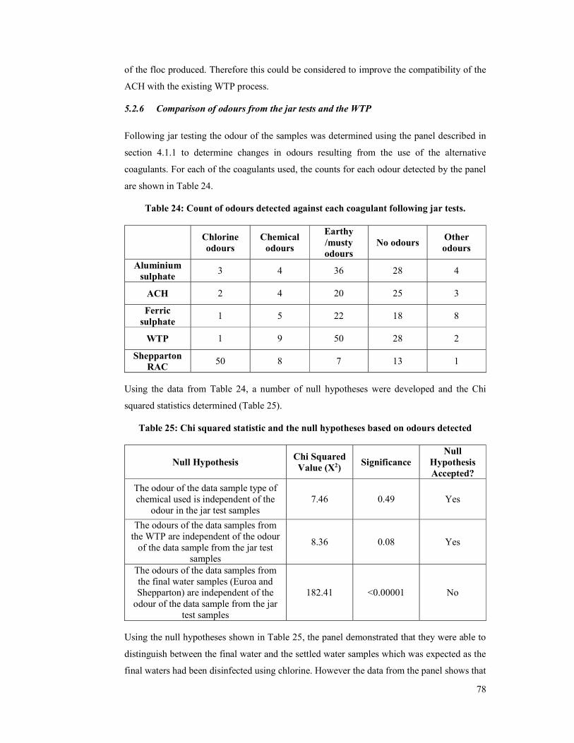
78

of the floc produced. Therefore this could be considered to improve the compatibility of the

ACH with the existing WTP process.

5.2.6 Comparison of odours from the jar tests and the WTP

Following jar testing the odour of the samples was determined using the panel described in

section 4.1.1 to determine changes in odours resulting from the use of the alternative

coagulants. For each of the coagulants used, the counts for each odour detected by the panel

are shown in Table 24.

Table 24: Count of odours detected against each coagulant following jar tests.

Chlorine odours

Chemical odours

Earthy /musty odours

No odours Other odours

Aluminium sulphate

3 4 36 28 4

ACH 2 4 20 25 3

Ferric sulphate

1 5 22 18 8

WTP 1 9 50 28 2

Shepparton RAC

50 8 7 13 1

Using the data from Table 24, a number of null hypotheses were developed and the Chi

squared statistics determined (Table 25).

Table 25: Chi squared statistic and the null hypotheses based on odours detected

Null Hypothesis Chi Squared Value (X2)

Significance Null

Hypothesis Accepted?

The odour of the data sample type of chemical used is independent of the

odour in the jar test samples 7.46 0.49 Yes

The odours of the data samples from the WTP are independent of the odour

of the data sample from the jar test samples

8.36 0.08 Yes

The odours of the data samples from the final water samples (Euroa and Shepparton) are independent of the

odour of the data sample from the jar test samples

182.41 <0.00001 No

Using the null hypotheses shown in Table 25, the panel demonstrated that they were able to

distinguish between the final water and the settled water samples which was expected as the

final waters had been disinfected using chlorine. However the data from the panel shows that

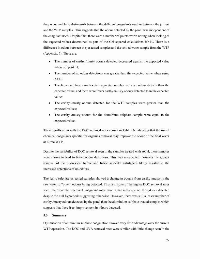
79

they were unable to distinguish between the different coagulants used or between the jar test

and the WTP samples. This suggests that the odour detected by the panel was independent of

the coagulant used. Despite this, there were a number of points worth noting when looking at

the expected values determined as part of the Chi squared calculations for H0 There is a

difference in odour between the jar tested samples and the settled water sample from the WTP

(Appendix 5). These are:

The number of earthy /musty odours detected decreased against the expected value

when using ACH;

The number of no odour detections was greater than the expected value when using

ACH;

The ferric sulphate samples had a greater number of other odour detects than the

expected value, and there were fewer earthy /musty odours detected than the expected

value;

The earthy /musty odours detected for the WTP samples were greater than the

expected values;

The earthy /musty odours for the aluminium sulphate sample were equal to the

expected value.

These results align with the DOC removal rates shown in Table 16 indicating that the use of

chemical coagulants specific for organics removal may improve the odour of the final water

at Euroa WTP.

Despite the variability of DOC removal seen in the samples treated with ACH, these samples

were shown to lead to fewer odour detections. This was unexpected, however the greater

removal of the fluorescent humic and fulvic acid-like substances likely assisted in the

increased detections of no odours.

The ferric sulphate jar tested samples showed a change in odours from earthy /musty in the

raw water to “other” odours being detected. This is in spite of the higher DOC removal rates

seen, therefore the chemical coagulant may have some influence on the odours detected

despite the null hypothesis suggesting otherwise. However, there was still a lesser number of

earthy /musty odours detected by the panel than the aluminium sulphate treated samples which

suggests that there is an improvement in odours detected.

5.3 Summary

Optimisation of aluminium sulphate coagulation showed very little advantage over the current

WTP operation. The DOC and UVA removal rates were similar with little change seen in the

80

fluorescent humic and fulvic acid – like substances. The odours were similar to the WTP with

earthy /musty odours still being the main odour detected. The LC-OCDs showed a different

pattern from the WTP sample, with the WTP sample showing a large reduction in humic

substances whereas the chromatograms for the aluminium sulphate sample showed a

significant concentration of residual humics.

The sludge density from the ACH coagulation is considered to be too low to work suitably in

the existing clarifier. However, in all other aspects ACH is considered a good option as the

data indicates that its use at the WTP would reduce odours as well as decrease the DOC

concentrations and reducing the formation of THMs. Through the use of the EEM spectra the

content of fluorescent humic and fulvic acid - like substances was shown to be reduced.

Coagulation with ferric sulphate was similar to that with ACH with respect to DOC and UVA

removal. The sludge volumes indicated that the sludge was heavy and would work very well

with the existing clarifier. The odour results showed that there was a change in odour, however

the panel were not clear if this was positive or negative in comparison to the existing odours

resulting from the WTP treatment process. Similar to the ACH the EEMs demonstrated a

reduction in fluorescent humic and fulvic acid- like substances.

Based on the overall improvement in odour, and the reduction in organic matter, both ACH

and ferric sulphate are considered superior to aluminium sulphate for coagulation. With

respect to the operation of the WTP the use of ferric sulphate is considered to be the most

appropriate option.

Before any final recommendations could be made a TBL assessment was conducted on the

various options for improvement of taste and odour issues at Euroa. The outcomes of these

are described in the next chapter.

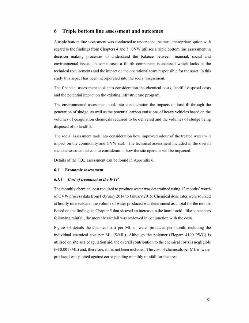
81

6 Triple bottom line assessment and outcomes

A triple bottom line assessment was conducted to understand the most appropriate option with

regard to the findings from Chapters 4 and 5. GVW utilises a triple bottom line assessment in

decision making processes to understand the balance between financial, social and

environmental issues. In some cases a fourth component is assessed which looks at the

technical requirements and the impact on the operational team responsible for the asset. In this

study this aspect has been incorporated into the social assessment.

The financial assessment took into consideration the chemical costs, landfill disposal costs

and the potential impact on the existing infrastructure program.

The environmental assessment took into consideration the impacts on landfill through the

generation of sludge, as well as the potential carbon emissions of heavy vehicles based on the

volumes of coagulation chemicals required to be delivered and the volumes of sludge being

disposed of to landfill.

The social assessment took into consideration how improved odour of the treated water will

impact on the community and GVW staff. The technical assessment included in the overall

social assessment takes into consideration how the site operator will be impacted.

Details of the TBL assessment can be found in Appendix 6.

6.1 Economic assessment

6.1.1 Cost of treatment at the WTP

The monthly chemical cost required to produce water was determined using 12 months’ worth

of GVW process data from February 2014 to January 2015. Chemical dose rates were sourced

at hourly intervals and the volume of water produced was determined as a total for the month.

Based on the findings in Chapter 5 that showed an increase in the humic acid - like substances

following rainfall, the monthly rainfall was reviewed in conjunction with the costs.

Figure 34 details the chemical cost per ML of water produced per month, including the

individual chemical cost per ML ($/ML). Although the polymer (Flopam 4190 PWG) is

utilised on site as a coagulation aid, the overall contribution to the chemical costs is negligible

(~$0.001 /ML) and, therefore, it has not been included. The cost of chemicals per ML of water

produced was plotted against corresponding monthly rainfall for the area.

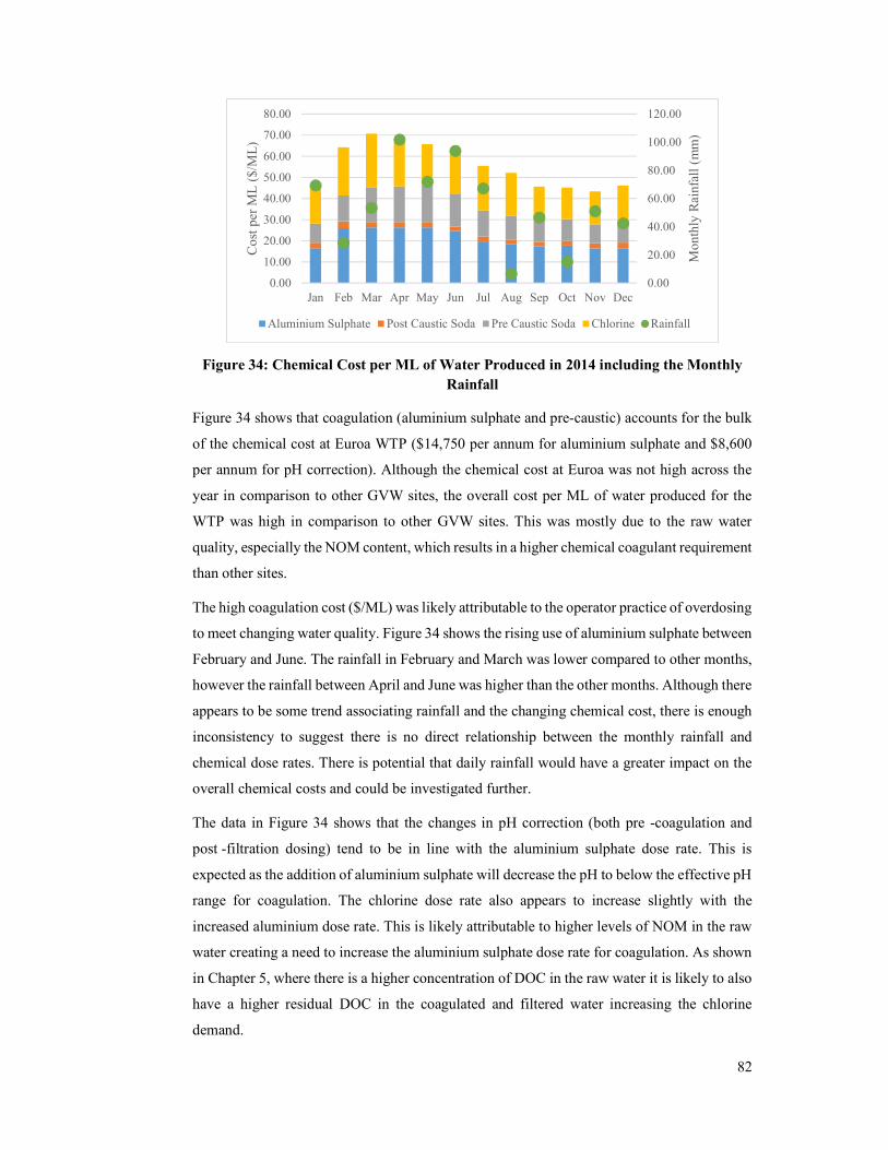
82

Figure 34: Chemical Cost per ML of Water Produced in 2014 including the Monthly Rainfall

Figure 34 shows that coagulation (aluminium sulphate and pre-caustic) accounts for the bulk

of the chemical cost at Euroa WTP ($14,750 per annum for aluminium sulphate and $8,600

per annum for pH correction). Although the chemical cost at Euroa was not high across the

year in comparison to other GVW sites, the overall cost per ML of water produced for the

WTP was high in comparison to other GVW sites. This was mostly due to the raw water

quality, especially the NOM content, which results in a higher chemical coagulant requirement

than other sites.

The high coagulation cost ($/ML) was likely attributable to the operator practice of overdosing

to meet changing water quality. Figure 34 shows the rising use of aluminium sulphate between

February and June. The rainfall in February and March was lower compared to other months,

however the rainfall between April and June was higher than the other months. Although there

appears to be some trend associating rainfall and the changing chemical cost, there is enough

inconsistency to suggest there is no direct relationship between the monthly rainfall and

chemical dose rates. There is potential that daily rainfall would have a greater impact on the

overall chemical costs and could be investigated further.

The data in Figure 34 shows that the changes in pH correction (both pre -coagulation and

post -filtration dosing) tend to be in line with the aluminium sulphate dose rate. This is

expected as the addition of aluminium sulphate will decrease the pH to below the effective pH

range for coagulation. The chlorine dose rate also appears to increase slightly with the

increased aluminium dose rate. This is likely attributable to higher levels of NOM in the raw

water creating a need to increase the aluminium sulphate dose rate for coagulation. As shown

in Chapter 5, where there is a higher concentration of DOC in the raw water it is likely to also

have a higher residual DOC in the coagulated and filtered water increasing the chlorine

demand.

0.00

20.00

40.00

60.00

80.00

100.00

120.00

0.00

10.00

20.00

30.00

40.00

50.00

60.00

70.00

80.00

Jan Feb Mar Apr May Jun Jul Aug Sep Oct Nov Dec

Mon

thly

Rai

nfal

l (m

m)

Cos

t per

ML

($/

ML

)

Aluminium Sulphate Post Caustic Soda Pre Caustic Soda Chlorine Rainfall

83

6.1.2 Potential cost of treatment based on jar test results

The average cost of treatment was determined for each chemical and compared to the WTP

cost (Figure 35). These data include the cost of post chemical dosing requirements of caustic

soda and chlorine.

Figure 35: The average chemical cost determined based on jar tests and the WTP dose

rates

The data presented in Figure 35 shows the average total cost of treatment per ML of water

produced with the mean for each chemical. These data correspond with the findings reported

in Chapter 5.2.1, showing that the average total cost per ML of water produced for aluminium

sulphate (N = 11, Std Dev = $5.22) is slightly less than the average WTP cost

(N = 11, Std Dev = $8.77). This supports the current site practices of overdosing to meet

changing water quality requirements. The post chemical dosing is the same for the WTP and

the aluminium sulphate jar test based on the final water quality.

ACH was determined as having the lowest average coagulant cost (N=12, Std Dev = $4.04),

which is due to not requiring pH correction for coagulation. The post chemical dosing was

shown to be similar to that for the WTP. The use of ACH provides good DOC removal and

odour testing results showed it to be cost effective. This does not include the slight increase

in polymer dosing costs (~$7.10 p.a.) or the potential costs of bentonite (~$284 p.a.) as these

are not considered as consequential in comparison to other chemical costs, and changing to

ACH, even when using bentonite, would still provide a financial benefit to GVW.

The use of ferric sulphate (N = 9, Std dev = $3.06) was shown to have a higher average cost

than aluminium sulphate. However the odours were determined to result in less earthy /musty

odours than using aluminium sulphate. As coagulation was undertaken at a lower pH (~pH 5)

than aluminium sulphate consideration was given to the impact of post filtration pH correction.

$39.60 $26.13

$37.74 $27.04

$15.38

$15.79 $19.64

$8.37

$2.87 $2.87

$2.87

$25.24

$25.24 $25.24 $25.24

$0.00$10.00$20.00$30.00$40.00$50.00$60.00$70.00$80.00$90.00

$100.00

Ferric Sulphate Aluminium sulphate ACH WTP

Cos

t of

chem

ical

s $/

ML

Chemical assessed

Coagulant Pre pH correction Post pH correction Chlorine

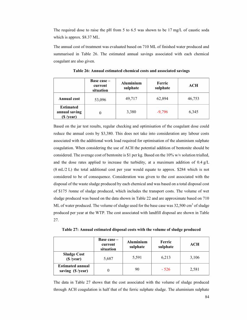
84

The required dose to raise the pH from 5 to 6.5 was shown to be 17 mg/L of caustic soda

which is approx. $8.37 ML.

The annual cost of treatment was evaluated based on 710 ML of finished water produced and

summarised in Table 26. The estimated annual savings associated with each chemical

coagulant are also given.

Table 26: Annual estimated chemical costs and associated savings

Base case – current

situation

Aluminium sulphate

Ferric sulphate

ACH

Annual cost 53,096 49,717 62,894 46,753

Estimated annual saving

($ /year) 0 3,380 -9,796 6,345

Based on the jar test results, regular checking and optimisation of the coagulant dose could

reduce the annual costs by $3,380. This does not take into consideration any labour costs

associated with the additional work load required for optimisation of the aluminium sulphate

coagulation. When considering the use of ACH the potential addition of bentonite should be

considered. The average cost of bentonite is $1 per kg. Based on the 10% w/v solution trialled,

and the dose rates applied to increase the turbidity, at a maximum addition of 0.4 g/L

(8 mL/2 L) the total additional cost per year would equate to approx. $284 which is not

considered to be of consequence. Consideration was given to the cost associated with the

disposal of the waste sludge produced by each chemical and was based on a total disposal cost

of $175 /tonne of sludge produced, which includes the transport costs. The volume of wet

sludge produced was based on the data shown in Table 22 and are approximate based on 710

ML of water produced. The volume of sludge used for the base case was 32,500 cm3 of sludge

produced per year at the WTP. The cost associated with landfill disposal are shown in Table

27.

Table 27: Annual estimated disposal costs with the volume of sludge produced

Base case – current

situation

Aluminium sulphate

Ferric sulphate

ACH

Sludge Cost ($ /year) 5,687 5,591 6,213 3,106

Estimated annual saving ($ /year) 0 90 - 526 2,581

The data in Table 27 shows that the cost associated with the volume of sludge produced

through ACH coagulation is half that of the ferric sulphate sludge. The aluminium sulphate

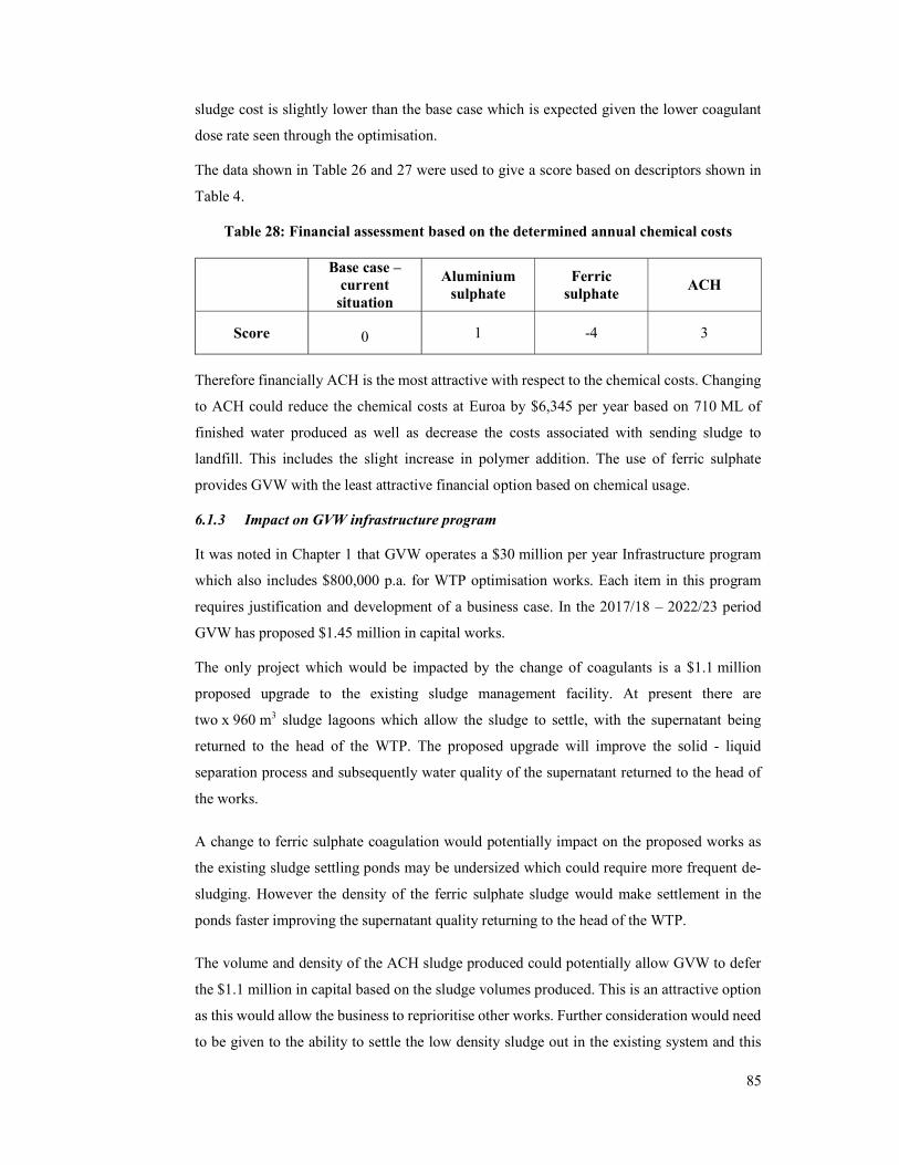
85

sludge cost is slightly lower than the base case which is expected given the lower coagulant

dose rate seen through the optimisation.

The data shown in Table 26 and 27 were used to give a score based on descriptors shown in

Table 4.

Table 28: Financial assessment based on the determined annual chemical costs

Base case – current

situation

Aluminium sulphate

Ferric sulphate

ACH

Score 0 1 -4 3

Therefore financially ACH is the most attractive with respect to the chemical costs. Changing

to ACH could reduce the chemical costs at Euroa by $6,345 per year based on 710 ML of

finished water produced as well as decrease the costs associated with sending sludge to

landfill. This includes the slight increase in polymer addition. The use of ferric sulphate

provides GVW with the least attractive financial option based on chemical usage.

6.1.3 Impact on GVW infrastructure program

It was noted in Chapter 1 that GVW operates a $30 million per year Infrastructure program

which also includes $800,000 p.a. for WTP optimisation works. Each item in this program

requires justification and development of a business case. In the 2017/18 – 2022/23 period

GVW has proposed $1.45 million in capital works.

The only project which would be impacted by the change of coagulants is a $1.1 million

proposed upgrade to the existing sludge management facility. At present there are

two x 960 m3 sludge lagoons which allow the sludge to settle, with the supernatant being

returned to the head of the WTP. The proposed upgrade will improve the solid - liquid

separation process and subsequently water quality of the supernatant returned to the head of

the works.

A change to ferric sulphate coagulation would potentially impact on the proposed works as

the existing sludge settling ponds may be undersized which could require more frequent de-

sludging. However the density of the ferric sulphate sludge would make settlement in the

ponds faster improving the supernatant quality returning to the head of the WTP.

The volume and density of the ACH sludge produced could potentially allow GVW to defer

the $1.1 million in capital based on the sludge volumes produced. This is an attractive option

as this would allow the business to reprioritise other works. Further consideration would need

to be given to the ability to settle the low density sludge out in the existing system and this

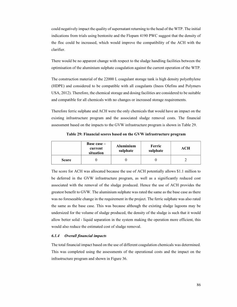
86

could negatively impact the quality of supernatant returning to the head of the WTP. The initial

indications from trials using bentonite and the Flopam 4190 PWC suggest that the density of

the floc could be increased, which would improve the compatibility of the ACH with the

clarifier.

There would be no apparent change with respect to the sludge handling facilities between the

optimisation of the aluminium sulphate coagulation against the current operation of the WTP.

The construction material of the 22000 L coagulant storage tank is high density polyethylene

(HDPE) and considered to be compatible with all coagulants (Ineos Olefins and Polymers

USA, 2012). Therefore, the chemical storage and dosing facilities are considered to be suitable

and compatible for all chemicals with no changes or increased storage requirements.

Therefore ferric sulphate and ACH were the only chemicals that would have an impact on the

existing infrastructure program and the associated sludge removal costs. The financial

assessment based on the impacts to the GVW infrastructure program is shown in Table 29.

Table 29: Financial scores based on the GVW infrastructure program

Base case –

current situation

Aluminium sulphate

Ferric sulphate

ACH

Score 0 0 0 2

The score for ACH was allocated because the use of ACH potentially allows $1.1 million to

be deferred in the GVW infrastructure program, as well as a significantly reduced cost

associated with the removal of the sludge produced. Hence the use of ACH provides the

greatest benefit to GVW. The aluminium sulphate was rated the same as the base case as there

was no foreseeable change in the requirement in the project. The ferric sulphate was also rated

the same as the base case. This was because although the existing sludge lagoons may be

undersized for the volume of sludge produced, the density of the sludge is such that it would

allow better solid - liquid separation in the system making the operation more efficient, this

would also reduce the estimated cost of sludge removal.

6.1.4 Overall financial impacts

The total financial impact based on the use of different coagulation chemicals was determined.

This was completed using the assessments of the operational costs and the impact on the

infrastructure program and shown in Figure 36.

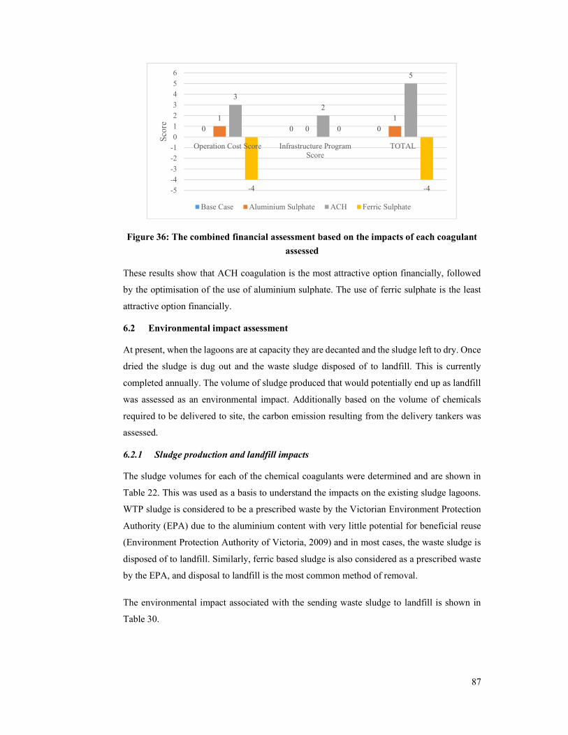
87

Figure 36: The combined financial assessment based on the impacts of each coagulant

assessed

These results show that ACH coagulation is the most attractive option financially, followed

by the optimisation of the use of aluminium sulphate. The use of ferric sulphate is the least

attractive option financially.

6.2 Environmental impact assessment

At present, when the lagoons are at capacity they are decanted and the sludge left to dry. Once

dried the sludge is dug out and the waste sludge disposed of to landfill. This is currently

completed annually. The volume of sludge produced that would potentially end up as landfill

was assessed as an environmental impact. Additionally based on the volume of chemicals

required to be delivered to site, the carbon emission resulting from the delivery tankers was

assessed.

6.2.1 Sludge production and landfill impacts

The sludge volumes for each of the chemical coagulants were determined and are shown in

Table 22. This was used as a basis to understand the impacts on the existing sludge lagoons.

WTP sludge is considered to be a prescribed waste by the Victorian Environment Protection

Authority (EPA) due to the aluminium content with very little potential for beneficial reuse

(Environment Protection Authority of Victoria, 2009) and in most cases, the waste sludge is

disposed of to landfill. Similarly, ferric based sludge is also considered as a prescribed waste

by the EPA, and disposal to landfill is the most common method of removal.

The environmental impact associated with the sending waste sludge to landfill is shown in

Table 30.

0 0 01

01

32

5

-4

0

-4-5-4-3-2-10123456

Operation Cost Score Infrastructure ProgramScore

TOTAL

Scor

e

Base Case Aluminium Sulphate ACH Ferric Sulphate

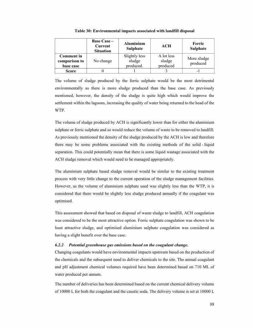
88

Table 30: Environmental impacts associated with landfill disposal

Base Case –

Current Situation

Aluminium Sulphate

ACH Ferric

Sulphate

Comment in comparison to

base case No change

Slightly less sludge

produced.

A lot less sludge

produced

More sludge produced

Score 0 1 3 -1

The volume of sludge produced by the ferric sulphate would be the most detrimental

environmentally as there is more sludge produced than the base case. As previously

mentioned, however, the density of the sludge is quite high which would improve the

settlement within the lagoons, increasing the quality of water being returned to the head of the

WTP.

The volume of sludge produced by ACH is significantly lower than for either the aluminium

sulphate or ferric sulphate and so would reduce the volume of waste to be removed to landfill.

As previously mentioned the density of the sludge produced by the ACH is low and therefore

there may be some problems associated with the existing methods of the solid - liquid

separation. This could potentially mean that there is some liquid wastage associated with the

ACH sludge removal which would need to be managed appropriately.

The aluminium sulphate based sludge removal would be similar to the existing treatment

process with very little change to the current operation of the sludge management facilities.

However, as the volume of aluminium sulphate used was slightly less than the WTP, it is

considered that there would be slightly less sludge produced annually if the coagulant was

optimised.

This assessment showed that based on disposal of waste sludge to landfill, ACH coagulation

was considered to be the most attractive option. Ferric sulphate coagulation was shown to be

least attractive sludge, and optimised aluminium sulphate coagulation was considered as

having a slight benefit over the base case.

6.2.2 Potential greenhouse gas emissions based on the coagulant change.

Changing coagulants would have environmental impacts upstream based on the production of

the chemicals and the subsequent need to deliver chemicals to the site. The annual coagulant

and pH adjustment chemical volumes required have been determined based on 710 ML of

water produced per annum.

The number of deliveries has been determined based on the current chemical delivery volume

of 10000 L for both the coagulant and the caustic soda. The delivery volume is set at 10000 L

89

because access to the site is not possible for larger tankers. As previously mentioned the

existing chemical coagulant tanks are suitable for all of the chemical coagulants assessed. This

means that the chemical delivery arrangements would remain the same. The number of

deliveries and volumes of chemicals required per annum can be seen in Table 31.

Table 31: Annual chemical volume requirements and annual delivery requirements

Base case – current

situation

Aluminium Sulphate

Ferric Sulphate

ACH

Coagulant (L/ year) 66,619 64,361 47,115 19,849

Caustic soda (L/ year) 14,766 13,433 13,048 1,602

Deliveries required coagulant

7 7 5 2

Deliveries required caustic soda

2 2 2 1

The data shown in Table 31 indicates that there would need to be only two chemical deliveries

required per year if GVW were to change to using ACH as a coagulant. This would

significantly reduce the GHGs emitted associated with the deliveries.

The volume of aluminium sulphate used when optimised would be sufficiently similar to the

current operation for the number of deliveries to be the same.

The use of ferric sulphate as a coagulant would have fewer delivery requirements compared

to the current operation. Despite using less caustic soda as pH correction for coagulation, the

increased extent of the post pH correction using caustic soda would increase the volume of

caustic soda required to be similar to the current operation.

The CO2 emitted for each delivery was determined using a figure of 600 g of CO2 emitted per

km driven with a full tanker load, and 500 g of CO2 emitted per km driven with an empty

tanker (Seo, et al., 2016). Chemical manufacture is completed on the outskirts of Western

Melbourne and delivered approximately 180 km to Euroa. This figure was used to determine

the CO2 emissions assuming a full load to Euroa and an empty load returning to Melbourne.

Based on the number of deliveries required in Table 31, the total volume of emissions for each

coagulant was determined and is shown in Figure 37.

The same exercise was completed determining the GHGs emitted for the disposal of waste

sludge for each coagulant. The sludge is disposed to the Euroa Resource Recovery Precinct

which is situated 5.3 km from the WTP. The truck size was considered to hold 15,000 kg and

the values of CO2 emitted were based on Seo, et al., (2016). These results are shown in Figure

37.

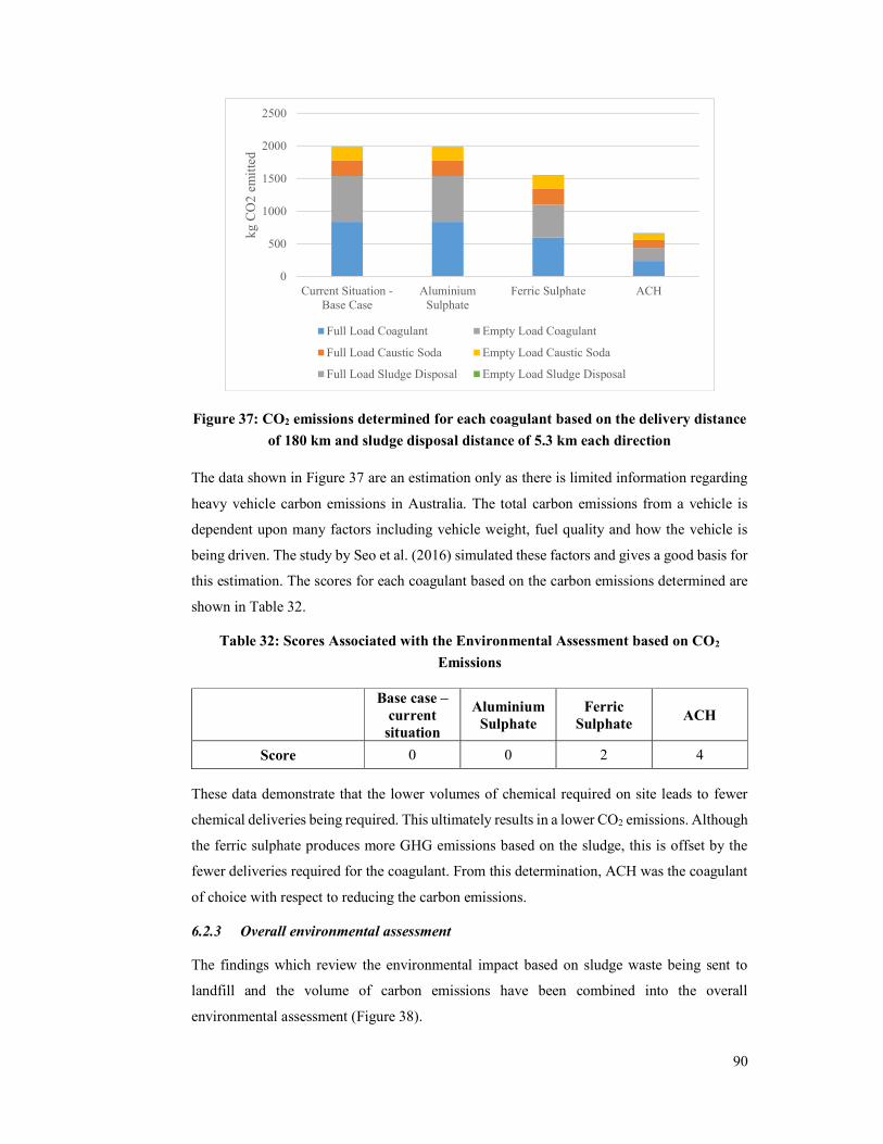
90

Figure 37: CO2 emissions determined for each coagulant based on the delivery distance

of 180 km and sludge disposal distance of 5.3 km each direction

The data shown in Figure 37 are an estimation only as there is limited information regarding

heavy vehicle carbon emissions in Australia. The total carbon emissions from a vehicle is

dependent upon many factors including vehicle weight, fuel quality and how the vehicle is

being driven. The study by Seo et al. (2016) simulated these factors and gives a good basis for

this estimation. The scores for each coagulant based on the carbon emissions determined are

shown in Table 32.

Table 32: Scores Associated with the Environmental Assessment based on CO2

Emissions

Base case – current

situation

Aluminium Sulphate

Ferric Sulphate

ACH

Score 0 0 2 4

These data demonstrate that the lower volumes of chemical required on site leads to fewer

chemical deliveries being required. This ultimately results in a lower CO2 emissions. Although

the ferric sulphate produces more GHG emissions based on the sludge, this is offset by the

fewer deliveries required for the coagulant. From this determination, ACH was the coagulant

of choice with respect to reducing the carbon emissions.

6.2.3 Overall environmental assessment

The findings which review the environmental impact based on sludge waste being sent to

landfill and the volume of carbon emissions have been combined into the overall

environmental assessment (Figure 38).

0

500

1000

1500

2000

2500

Current Situation -Base Case

AluminiumSulphate

Ferric Sulphate ACH

kg C

O2

emit

ted

Full Load Coagulant Empty Load Coagulant

Full Load Caustic Soda Empty Load Caustic Soda

Full Load Sludge Disposal Empty Load Sludge Disposal

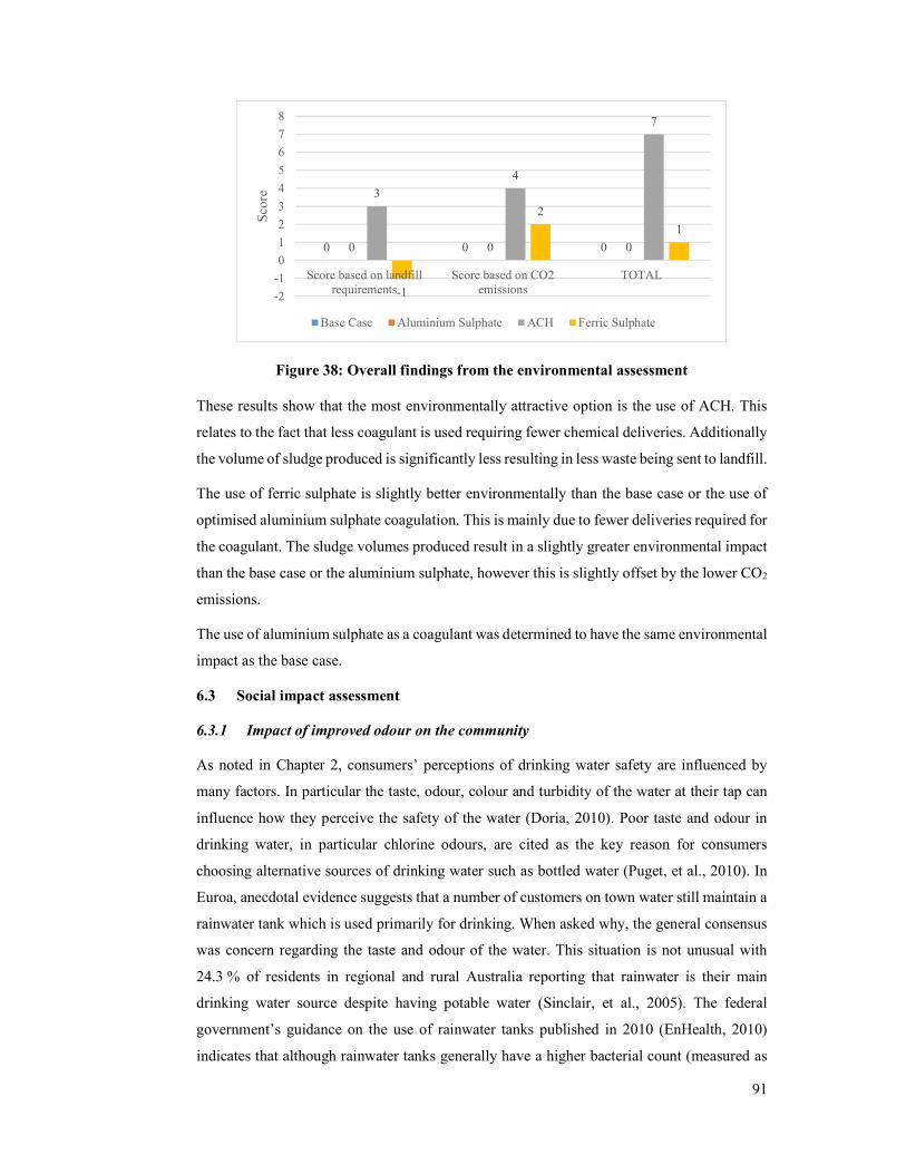
91

Figure 38: Overall findings from the environmental assessment

These results show that the most environmentally attractive option is the use of ACH. This

relates to the fact that less coagulant is used requiring fewer chemical deliveries. Additionally

the volume of sludge produced is significantly less resulting in less waste being sent to landfill.

The use of ferric sulphate is slightly better environmentally than the base case or the use of

optimised aluminium sulphate coagulation. This is mainly due to fewer deliveries required for

the coagulant. The sludge volumes produced result in a slightly greater environmental impact

than the base case or the aluminium sulphate, however this is slightly offset by the lower CO2

emissions.

The use of aluminium sulphate as a coagulant was determined to have the same environmental

impact as the base case.

6.3 Social impact assessment

6.3.1 Impact of improved odour on the community

As noted in Chapter 2, consumers’ perceptions of drinking water safety are influenced by

many factors. In particular the taste, odour, colour and turbidity of the water at their tap can

influence how they perceive the safety of the water (Doria, 2010). Poor taste and odour in

drinking water, in particular chlorine odours, are cited as the key reason for consumers

choosing alternative sources of drinking water such as bottled water (Puget, et al., 2010). In

Euroa, anecdotal evidence suggests that a number of customers on town water still maintain a

rainwater tank which is used primarily for drinking. When asked why, the general consensus

was concern regarding the taste and odour of the water. This situation is not unusual with

24.3 % of residents in regional and rural Australia reporting that rainwater is their main

drinking water source despite having potable water (Sinclair, et al., 2005). The federal

government’s guidance on the use of rainwater tanks published in 2010 (EnHealth, 2010)

indicates that although rainwater tanks generally have a higher bacterial count (measured as

0 0 00 0 0

3

4

7

-1

2

1

-2

-1

0

1

2

3

4

5

6

7

8

Score based on landfillrequirements

Score based on CO2emissions

TOTALSc

ore

Base Case Aluminium Sulphate ACH Ferric Sulphate

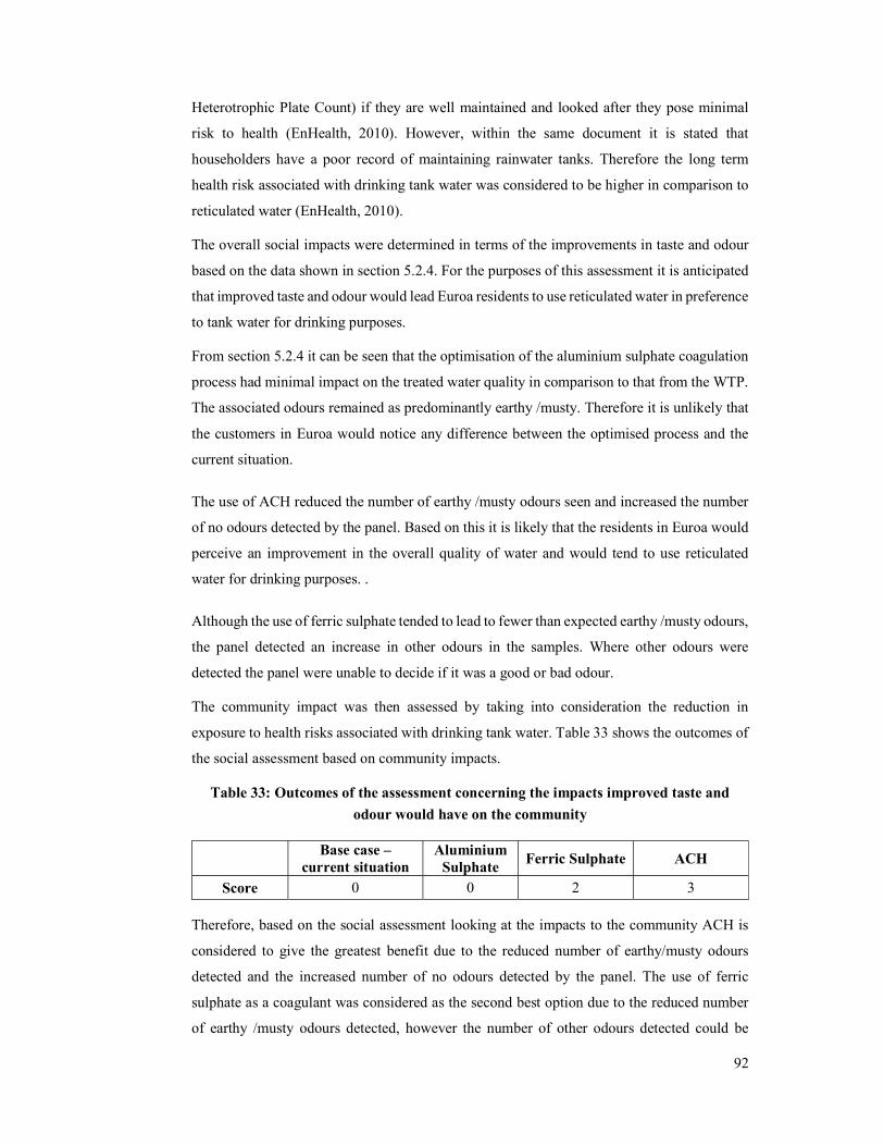
92

Heterotrophic Plate Count) if they are well maintained and looked after they pose minimal

risk to health (EnHealth, 2010). However, within the same document it is stated that

householders have a poor record of maintaining rainwater tanks. Therefore the long term

health risk associated with drinking tank water was considered to be higher in comparison to

reticulated water (EnHealth, 2010).

The overall social impacts were determined in terms of the improvements in taste and odour

based on the data shown in section 5.2.4. For the purposes of this assessment it is anticipated

that improved taste and odour would lead Euroa residents to use reticulated water in preference

to tank water for drinking purposes.

From section 5.2.4 it can be seen that the optimisation of the aluminium sulphate coagulation

process had minimal impact on the treated water quality in comparison to that from the WTP.

The associated odours remained as predominantly earthy /musty. Therefore it is unlikely that

the customers in Euroa would notice any difference between the optimised process and the

current situation.

The use of ACH reduced the number of earthy /musty odours seen and increased the number

of no odours detected by the panel. Based on this it is likely that the residents in Euroa would

perceive an improvement in the overall quality of water and would tend to use reticulated

water for drinking purposes. .

Although the use of ferric sulphate tended to lead to fewer than expected earthy /musty odours,

the panel detected an increase in other odours in the samples. Where other odours were

detected the panel were unable to decide if it was a good or bad odour.

The community impact was then assessed by taking into consideration the reduction in

exposure to health risks associated with drinking tank water. Table 33 shows the outcomes of

the social assessment based on community impacts.

Table 33: Outcomes of the assessment concerning the impacts improved taste and

odour would have on the community

Base case – current situation

Aluminium Sulphate

Ferric Sulphate ACH

Score 0 0 2 3

Therefore, based on the social assessment looking at the impacts to the community ACH is

considered to give the greatest benefit due to the reduced number of earthy/musty odours

detected and the increased number of no odours detected by the panel. The use of ferric

sulphate as a coagulant was considered as the second best option due to the reduced number

of earthy /musty odours detected, however the number of other odours detected could be

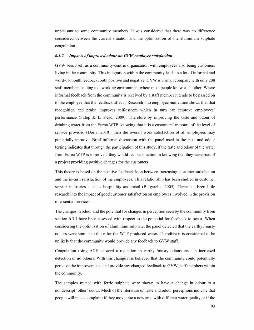
93

unpleasant to some community members. It was considered that there was no difference

considered between the current situation and the optimisation of the aluminium sulphate

coagulation.

6.3.2 Impacts of improved odour on GVW employee satisfaction

GVW sees itself as a community-centric organisation with employees also being customers

living in the community. This integration within the community leads to a lot of informal and

word-of-mouth feedback, both positive and negative. GVW is a small company with only 208

staff members leading to a working environment where most people know each other. Where

informal feedback from the community is received by a staff member it tends to be passed on

to the employee that the feedback affects. Research into employee motivation shows that that

recognition and praise improves self-esteem which in turn can improve employees’

performance (Fulop & Linstead, 2009). Therefore by improving the taste and odour of

drinking water from the Euroa WTP, knowing that it is a customers’ measure of the level of

service provided (Doria, 2010), then the overall work satisfaction of all employees may

potentially improve. Brief informal discussion with the panel used in the taste and odour

testing indicates that through the participation of this study, if the taste and odour of the water

from Euroa WTP is improved, they would feel satisfaction in knowing that they were part of

a project providing positive changes for the customers.

This theory is based on the positive feedback loop between increasing customer satisfaction

and the in-turn satisfaction of the employees. This relationship has been studied in customer

service industries such as hospitality and retail (Bulgarella, 2005). There has been little

research into the impact of good customer satisfaction on employees involved in the provision

of essential services.

The changes in odour and the potential for changes in perception seen by the community from

section 6.3.1 have been assessed with respect to the potential for feedback to occur. When

considering the optimisation of aluminium sulphate, the panel detected that the earthy /musty

odours were similar to those for the WTP produced water. Therefore it is considered to be

unlikely that the community would provide any feedback to GVW staff.

Coagulation using ACH showed a reduction in earthy /musty odours and an increased

detection of no odours. With this change it is believed that the community could potentially

perceive the improvements and provide any changed feedback to GVW staff members within

the community.

The samples treated with ferric sulphate were shown to have a change in odour to a

nondescript ‘other’ odour. Much of the literature on taste and odour perceptions indicate that

people will make complaint if they move into a new area with different water quality or if the

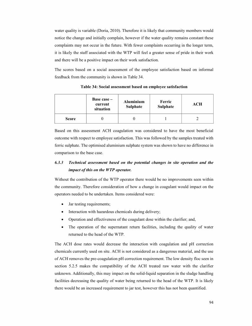
94

water quality is variable (Doria, 2010). Therefore it is likely that community members would

notice the change and initially complain, however if the water quality remains constant these

complaints may not occur in the future. With fewer complaints occurring in the longer term,

it is likely the staff associated with the WTP will feel a greater sense of pride in their work

and there will be a positive impact on their work satisfaction.

The scores based on a social assessment of the employee satisfaction based on informal

feedback from the community is shown in Table 34.

Table 34: Social assessment based on employee satisfaction

Base case – current

situation

Aluminium Sulphate

Ferric Sulphate

ACH

Score 0 0 1 2

Based on this assessment ACH coagulation was considered to have the most beneficial

outcome with respect to employee satisfaction. This was followed by the samples treated with

ferric sulphate. The optimised aluminium sulphate system was shown to have no difference in

comparison to the base case.

6.3.3 Technical assessment based on the potential changes in site operation and the

impact of this on the WTP operator.

Without the contribution of the WTP operator there would be no improvements seen within

the community. Therefore consideration of how a change in coagulant would impact on the

operators needed to be undertaken. Items considered were:

Jar testing requirements;

Interaction with hazardous chemicals during delivery;

Operation and effectiveness of the coagulant dose within the clarifier; and,

The operation of the supernatant return facilities, including the quality of water

returned to the head of the WTP.

The ACH dose rates would decrease the interaction with coagulation and pH correction

chemicals currently used on site. ACH is not considered as a dangerous material, and the use

of ACH removes the pre-coagulation pH correction requirement. The low density floc seen in

section 5.2.5 makes the compatibility of the ACH treated raw water with the clarifier

unknown. Additionally, this may impact on the solid-liquid separation in the sludge handling

facilities decreasing the quality of water being returned to the head of the WTP. It is likely

there would be an increased requirement to jar test, however this has not been quantified.

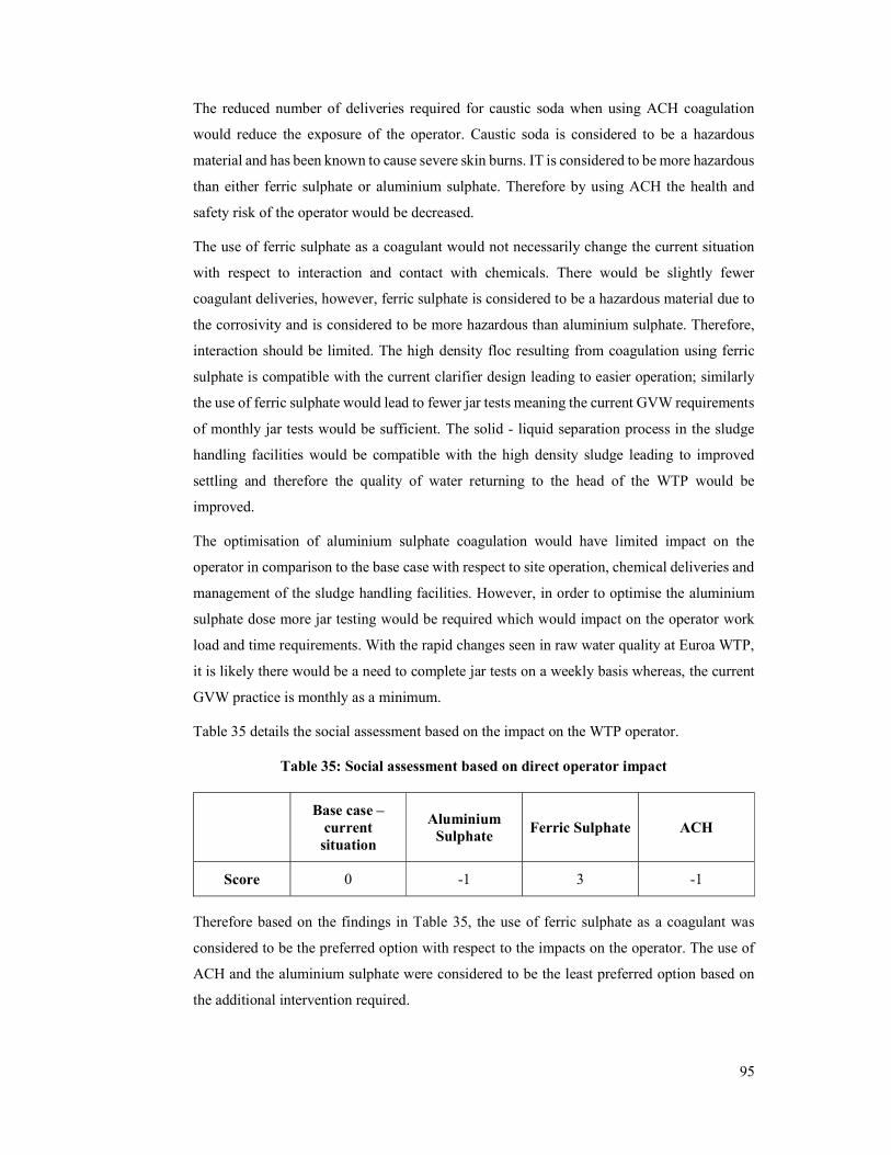
95

The reduced number of deliveries required for caustic soda when using ACH coagulation

would reduce the exposure of the operator. Caustic soda is considered to be a hazardous

material and has been known to cause severe skin burns. IT is considered to be more hazardous

than either ferric sulphate or aluminium sulphate. Therefore by using ACH the health and

safety risk of the operator would be decreased.

The use of ferric sulphate as a coagulant would not necessarily change the current situation

with respect to interaction and contact with chemicals. There would be slightly fewer

coagulant deliveries, however, ferric sulphate is considered to be a hazardous material due to

the corrosivity and is considered to be more hazardous than aluminium sulphate. Therefore,

interaction should be limited. The high density floc resulting from coagulation using ferric

sulphate is compatible with the current clarifier design leading to easier operation; similarly

the use of ferric sulphate would lead to fewer jar tests meaning the current GVW requirements

of monthly jar tests would be sufficient. The solid - liquid separation process in the sludge

handling facilities would be compatible with the high density sludge leading to improved

settling and therefore the quality of water returning to the head of the WTP would be

improved.

The optimisation of aluminium sulphate coagulation would have limited impact on the

operator in comparison to the base case with respect to site operation, chemical deliveries and

management of the sludge handling facilities. However, in order to optimise the aluminium

sulphate dose more jar testing would be required which would impact on the operator work

load and time requirements. With the rapid changes seen in raw water quality at Euroa WTP,

it is likely there would be a need to complete jar tests on a weekly basis whereas, the current

GVW practice is monthly as a minimum.

Table 35 details the social assessment based on the impact on the WTP operator.

Table 35: Social assessment based on direct operator impact

Base case – current

situation

Aluminium Sulphate

Ferric Sulphate ACH

Score 0 -1 3 -1

Therefore based on the findings in Table 35, the use of ferric sulphate as a coagulant was

considered to be the preferred option with respect to the impacts on the operator. The use of

ACH and the aluminium sulphate were considered to be the least preferred option based on

the additional intervention required.

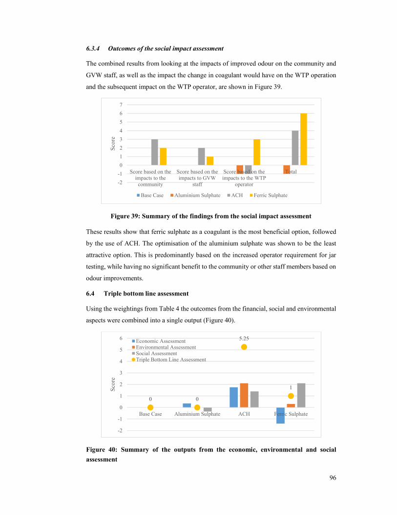
96

6.3.4 Outcomes of the social impact assessment

The combined results from looking at the impacts of improved odour on the community and

GVW staff, as well as the impact the change in coagulant would have on the WTP operation

and the subsequent impact on the WTP operator, are shown in Figure 39.

Figure 39: Summary of the findings from the social impact assessment

These results show that ferric sulphate as a coagulant is the most beneficial option, followed

by the use of ACH. The optimisation of the aluminium sulphate was shown to be the least

attractive option. This is predominantly based on the increased operator requirement for jar

testing, while having no significant benefit to the community or other staff members based on

odour improvements.

6.4 Triple bottom line assessment

Using the weightings from Table 4 the outcomes from the financial, social and environmental

aspects were combined into a single output (Figure 40).

Figure 40: Summary of the outputs from the economic, environmental and social

assessment

-2

-1

0

1

2

3

4

5

6

7

Score based on theimpacts to the

community

Score based on theimpacts to GVW

staff

Score based on theimpacts to the WTP

operator

Total

Scor

e

Base Case Aluminium Sulphate ACH Ferric Sulphate

0 0

5.25

1

-2

-1

0

1

2

3

4

5

6

Base Case Aluminium Sulphate ACH Ferric Sulphate

Scor

e

Economic AssessmentEnvironmental AssessmentSocial AssessmentTriple Bottom Line Assessment

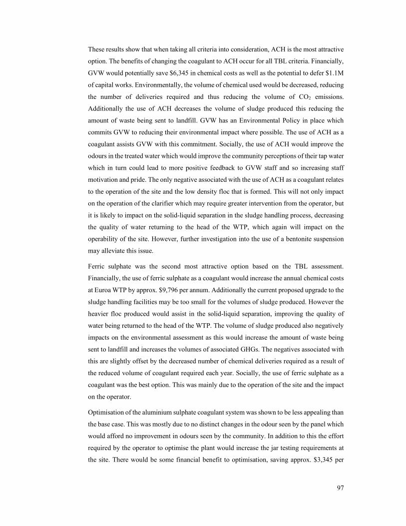
97

These results show that when taking all criteria into consideration, ACH is the most attractive

option. The benefits of changing the coagulant to ACH occur for all TBL criteria. Financially,

GVW would potentially save $6,345 in chemical costs as well as the potential to defer $1.1M

of capital works. Environmentally, the volume of chemical used would be decreased, reducing

the number of deliveries required and thus reducing the volume of CO2 emissions.

Additionally the use of ACH decreases the volume of sludge produced this reducing the

amount of waste being sent to landfill. GVW has an Environmental Policy in place which

commits GVW to reducing their environmental impact where possible. The use of ACH as a

coagulant assists GVW with this commitment. Socially, the use of ACH would improve the

odours in the treated water which would improve the community perceptions of their tap water

which in turn could lead to more positive feedback to GVW staff and so increasing staff

motivation and pride. The only negative associated with the use of ACH as a coagulant relates

to the operation of the site and the low density floc that is formed. This will not only impact

on the operation of the clarifier which may require greater intervention from the operator, but

it is likely to impact on the solid-liquid separation in the sludge handling process, decreasing

the quality of water returning to the head of the WTP, which again will impact on the

operability of the site. However, further investigation into the use of a bentonite suspension

may alleviate this issue.

Ferric sulphate was the second most attractive option based on the TBL assessment.

Financially, the use of ferric sulphate as a coagulant would increase the annual chemical costs

at Euroa WTP by approx. $9,796 per annum. Additionally the current proposed upgrade to the

sludge handling facilities may be too small for the volumes of sludge produced. However the

heavier floc produced would assist in the solid-liquid separation, improving the quality of

water being returned to the head of the WTP. The volume of sludge produced also negatively

impacts on the environmental assessment as this would increase the amount of waste being

sent to landfill and increases the volumes of associated GHGs. The negatives associated with

this are slightly offset by the decreased number of chemical deliveries required as a result of

the reduced volume of coagulant required each year. Socially, the use of ferric sulphate as a

coagulant was the best option. This was mainly due to the operation of the site and the impact

on the operator.

Optimisation of the aluminium sulphate coagulant system was shown to be less appealing than

the base case. This was mostly due to no distinct changes in the odour seen by the panel which

would afford no improvement in odours seen by the community. In addition to this the effort

required by the operator to optimise the plant would increase the jar testing requirements at

the site. There would be some financial benefit to optimisation, saving approx. $3,345 per

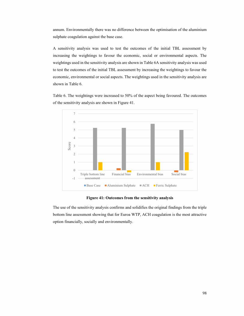
98

annum. Environmentally there was no difference between the optimisation of the aluminium

sulphate coagulation against the base case.

A sensitivity analysis was used to test the outcomes of the initial TBL assessment by

increasing the weightings to favour the economic, social or environmental aspects. The

weightings used in the sensitivity analysis are shown in Table 6A sensitivity analysis was used

to test the outcomes of the initial TBL assessment by increasing the weightings to favour the

economic, environmental or social aspects. The weightings used in the sensitivity analysis are

shown in Table 6.

Table 6. The weightings were increased to 50% of the aspect being favoured. The outcomes

of the sensitivity analysis are shown in Figure 41.

Figure 41: Outcomes from the sensitivity analysis

The use of the sensitivity analysis confirms and solidifies the original findings from the triple

bottom line assessment showing that for Euroa WTP, ACH coagulation is the most attractive

option financially, socially and environmentally.

-1

0

1

2

3

4

5

6

7

Triple bottom lineassessment

Financial bias Environmental bias Social bias

Scor

e

Base Case Aluminium Sulphate ACH Ferric Sulphate

99

7 Conclusions and recommendations of further work

This chapter provides a summary of the case study reflecting on the research questions posed

in Chapter 1. Further to this, recommendations of further work required resulting from this

research were made.

7.1 Conclusions

Through the use of a taste and odour panel the predominant odours of the water treated by

Euroa WTP were determined as earthy /musty and chlorinous, whereas no specific tastes were

detected.

The presence of earthy /musty odours in the reticulation system suggested that geosmin and

MIB may be present however, there were no detections above the odour detection limit

disproving the theory that these were responsible for the earthy/musty odours. The free

chlorine residual seen at the WTP was consistently above the aesthetic limit for chlorine and

was considered the cause of the chlorine odours detected.

Correlation of water quality parameters to odours detected by the panel showed that SUVA

provides an indication where an earthy musty or chlorinous odour may occur. DOC and UVA

were shown to have a non-linear relationship with the odours. There appeared to be an

optimum point where fewer odours were detected, this was at UVA = 0.48 /cm and

DOC = 12 mg/L. DOC is currently determined through SGS Laboratories, whereas UVA or

UVT can be measured on site using a bench top analyser. In order to give the operator an

understanding of the characteristics of the NOM present in the water, a linear relationship

between the UVA and DOC concentration was developed. This was determined to be:

DOC = 13.4UVA + 1.2

As expected, the free chlorine residual related back to the chlorinous odours detected.

However it was stronger at the point of disinfection than on the outlet of the storage. There

was also a linear relationship between the earthy /musty odours detected and the free chlorine

residual.

Therefore the use of SUVA, DOC, UVA and free chlorine are useful tools for the operator at

Euroa WTP to determine where a taste and odour issue may occur and so enable the treatment

process to be optimised for organics removal.

In order to assist the operator with the optimisation, an equation to determine the aluminium

sulphate dose was developed using turbidity and UVT. This equation was determined as:

Aluminium sulphate dose rate (mg/L) = 141.4 – 0.86UVT – 0.71Turbidity

100

However, optimisation of the aluminium sulphate coagulation for DOC removal showed no

change in the odours detected with earthy /musty being the predominant odours detected by

the panel. In addition to this the DOC removal rates through jar testing showed to be slightly

less than the WTP (55 % and 57 % respectively). Therefore, it is unlikely that the optimisation

of the aluminium sulphate coagulation would provide any benefit with respect to the odours

detected by the community.

Optimisation of the aluminium sulphate coagulation would result in a financial saving of

$3,380 per year for chemicals and $90 per year for sludge disposal when compared to the

current WTP operation. There would be no impact on the existing GVW infrastructure

program resulting from the optimisation. There would be minimal environmental benefit to

optimising the aluminium sulphate with no change in GHG emissions from chemical

deliveries compared to the current operation. However, there would be a slight reduction in

the amount of sludge sent to landfill through optimisation. With respect to the social benefits,

there appeared to be no clear benefit to the community or staff members. The overall impact

of optimising the aluminium sulphate coagulation on the operator would be greater than the

current operation, as there would be an increased jar testing requirement.

The use of ferric sulphate was shown to have environmental and social benefits, however it

was considered to be economically disadvantageous. Using ferric sulphate as a coagulant gave

a higher DOC removal rate than the WTP (72 % and 57 %, respectively). The sludge produced

using ferric sulphate was heavy and settled well, which indicates it would work well within

the WTP potentially improving the performance of the clarifier. Following jar testing, the

panel determined that there were more other odour detects than the expected value, however

there were also fewer earthy /musty odours than the expected value indicating that the use of

ferric sulphate would decrease the number of odours detected in the Euroa community.

Financially the use of ferric sulphate would increase the annual chemical costs by $9,796 and

with the increased volume of sludge produced, there would be an annual increase in sludge

disposal costs by $526. There is no ability to defer any current infrastructure projects.

Environmentally, the use of ferric sulphate would reduce the GHG emissions associated with

chemical deliveries in comparison to the WTP. Conversely, the volume of sludge being

disposed of to landfill would increase, however, as the density of the sludge produced is

greater than the aluminium based sludge, the solid liquid separation in the sludge handling

facility would be improved. Socially the reduced number of earthy /musty odours detected

would see benefits to the community. This would in turn improve feedback provided to GVW

staff improving morale and motivation. The use of ferric sulphate as a coagulant was

considered to be the most advantageous to the WTP operator as it appears to be compatible

101

with the existing clarifier and sludge handling facilities. This would potentially improve the

process reducing the interaction required by the operator.

The use of ACH as a coagulant proved to have economic, environmental and social benefits.

Using ACH as a coagulant gave a higher DOC removal rate than the WTP (59 % and 57%,

respectively). However, the sludge produced using ACH was of low density with floc

remaining in suspension following settling. Initial experiments showed that the use of a

polymer and a bentonite suspension to increase turbidity would improve the sludge density

and settlement. Following jar testing, the panel determined that there were more no odour

detections than the expected value, indicating that the use of ACH would decrease the number

of odours detected in the Euroa community.

Financially the use of ACH would decrease the annual chemical costs by $6,345 and with the

reduced volume of sludge produced, there would be an annual saving of $2,581 based on the

reduced sludge disposal requirements. In addition to this, the reduced sludge volumes could

result in the deferral of a $1.1 million upgrade to the existing sludge handling facilities.

Environmentally, the use of ACH would reduce the GHG emissions associated with chemical

deliveries and the volume of sludge being disposed of to landfill would be reduced. Socially

the improved odours would see benefits to the community which in turn would improve

feedback being given to GVW staff improving morale and motivation. However, the use of

ACH may cause some operational issues at the WTP based on the low density sludge. As

previously mentioned the initial results from trials with bentonite are positive which would

reduce this impact on the WTP operator.

Therefore the use of alternative coagulants would improve the odours detected by the Euroa

community, whilst providing social and environmental benefits to GVW. The use of ACH

would provide a financial benefit whereas the use of ferric sulphate would increase the

chemical and sludge disposal costs to the business.

GVW should reconsider the use of aluminium sulphate at Euroa WTP and investigate the use

of ACH as a chemical coagulant further as ACH provides financial, social and environmental

benefits,

7.2 Recommendations of further work

This case study was based on specific findings from Euroa WTP. The presence of NOM within

the raw water was found to be the key source of taste and odours in the reticulation system.

By using alternative coagulants, it was determined that the taste and odour of drinking water

could be improved whilst improving social, environmental and economic aspects of the

102

business. From this study some further research opportunities and further work were identified

for GVW.

Firstly as taste and odour is becoming an increased focus to GVW due to its customer centric

direction, further emphasis should be placed on understanding the tastes and odours in the

drinking water systems. This should also include the perceptions of the wider community of

the taste and odour of their drinking water. In addition, the WTP operators should undertake

further training to understand the importance of taste and odour in drinking water.

The case study showed that the operator’s main focus was not primarily on organics removal,

however there was an awareness of the impact of organics on the treatment process. It is

recommended that DOC analysers be installed on the raw water line at Euroa, and the use of

SUVA be employed to identify where there may be taste and odours present in the reticulation

system to enable adjustment of the chemical coagulation process accordingly. There is

potential to develop a training and guidance manual around the management of chemical

coagulation for NOM removal and taste and odour improvement.

ACH proved to be the most beneficial coagulant for Euroa WTP when social, environmental

and economic parameters were considered, however there were some concerns regarding the

compatibility with the existing WTP. Initial results showed that the use of Flopam 4190 PWC

and bentonite improved the settling of the floc. It is recommended that the further investigation

and lab trials into other polymers and bentonite addition should be completed prior to a plant

trial.

On a wider note it is suggested that further research be undertaken into the impact of different

chemical coagulants on odours in the treated water.

Finally it is recommended that the methodology and approach used in this research be

extended to other GVW sites to understand if taste and odours issues in other areas can be

predicted by a WTP operator based on simple water quality parameters.

103

References

Adams, C., Muir, S. & Hoque, Z., 2014. Measurement of Sustainability Performance in the

Public Sector. Sustainability, Accounting, Management and Policy Journal, 5(1), pp. 46-67.

Alvarez-Gaitan, J. P. et al., 2013. A Hybrid Life Cycle Assessment of Water Treatment

Chemicals. International Journal of Life Cycle Assessment , Volume 18, pp. 1291 - 1301.

Antonopoulou, M., Evgenidou, E., Lambropoulou, D. & Konstantinou, I., 2014. A review on

advanced oxidation processes for the removal of taste and odour compounds from aqueous

media. Water Research, Volume 53, pp. 215 - 234.

Ates, N., Kitis, M. & Yetis, U., 2007. Formation of Chlorination by- Products in Waters with

Low SUVA - Correlations with SUVA and Differential UV Spectroscopy. Water Research,

Volume 41, pp. 4139 - 4148.

Bae, B. et al., 2002. Demonstration of New Sensory Methods for Drinking Water Taste and

Odour Control. Water Science and Technology, 2(5-6), pp. 241-247.

Bartels, J., Burlingame, G. & Suffet, I., 1986. Flavour Profile Analysis: Taste and Odour

Control of the Future. Journal (American Water Works Association), Volume 78, pp. 50-55.

Benvenuti, J., 2011. Customer Expectations - Service Standards in the Next Regulatory Period

and Beyond. Melbourne Australia, Essential Services Commission.

Bond, T., Goslan, E., Parsons, S. & Jefferson, B., 2012. A critical review of trihalomethane

and haloacetic acid formation from natural organic matter surrogates. Environmental

Technology Reviews, 1(1), pp. 93-113.

Bruchet, A., Duguet, J. & Suffet, I., 2004. Role of Oxidants and Disinfectants on the Removal,

Masking and Generation of Tastes and Odours. Reviews in Environmental Science and

Biotechnology, Volume 3, pp. 33-41.

Bulgarella, C. C., 2005. Employee Satisfaction & Customer Satisfaction: Is there a

relationship?, s.l.: Guide Star Research for Better Business Relationships.

Burlingame, G., Dietrich, A. & Whelton, A., 2007. Understanding the Basics of Tap Water.

Journal (American Water Works Association) , Volume 99, pp. 100-111.

Burlingame, G., Doty, R. & Dietrich, A., 2017. Humans as Sensors to Evaluate Drinking

Water Taste and Odour: A Review. Journal of the American Water Works Association, p. In

Press.

104

Chang, E., Chiang, P., Chao, S. & Lin, Y., 2006. Relationship between Chlorine Consumption

and Chlorination by Products Formation for Model Compounds. Chemosphere, Volume 64,

pp. 1196-1203.

Chebat, J., Davidow, M. & Codjovi, I., 2005. Silent Voices:Why Some Dissatisfied

Consumers Fail to Complain. Journal of Service Research, 7(4), pp. 328-342.

Chen, W., Westerhoff, P., Leenheer, J. A. & Booksh, K., 2003. Fluorescence Excitation-

Emission Matrix Regional Integration to Quantify Spectra for Dissolved Organic Matter.

Environmental Science and Technology, 37(24), pp. 5701-5710.

Comrie, D., Evans, S., Gale, R. & Kitney, P., 2002. Taste and Odour in Drinking Water:

Perception Versus Reality. Water (Australia), Volume 29, pp. 20-24.

Deborde, M. & Van Gunten, U., 2008. Reactions of Chlorine With Inorganic and Organic

Compounds During Water Treatment - Kinetics and Mechanisms: A Critical Review. Water

Research, Volume 42, pp. 13-51.

Dietrich, A., 2006. Aesthetic Issues for Drinking Water. Journal of Water and Health, Volume

4, pp. 11-16.

Dietrich, A. et al., 1995. Oxidation of Odourous and Nonodourous Algal Metabolites by

Permanganate, Chlorine and Chlorine DIoxide. Water Science and Technology, Volume 31,

pp. 223 - 228.

Doria, M., 2006. Bottled Water Versus Tap Water: Understanding Consumers Preferences.

Journal of Water and Health, 4(2), pp. 271-276.

Doria, M., 2010. Factors Influencing Public Perception of Drinking Water Quality. Water

Policy, Volume 12, pp. 1-9.

Doria, M., Pidgeon, N. & Hunter, P., 2009. Perceptions of Drinking Water Quality and Risk

and Its Effect on Behaviour: A Cross National Study. Science of the Total Environment,

407(21), pp. 5455-5464.

Drikas, M., 2003. Natural Organic Matter in Drinking Water: Problems and Solutions. Natural

Organic Matter in Drinking Water: Problems and Solutions, pp. 5-9.

Drikas, M., Dixon, M. & Morran, J., 2009. Removal of MIB and geosmin using granular

activated carbon with and without MIEX pre-treatment. Water Research, Volume 43, pp.

5151-5159.

Edzwald, J. & Kaminski, G. S., 2007. A Simple Method for Water Plant Optimisation and

Operation of Coagulation. s.l., American Water Works Association - WQTC Conference.

105

Edzwald, J. & Tobiason, J., 1999. Enhanced Coagulation: US Requiremetns and A Broader

View. Water Science and Technology, 40(9), pp. 63-70.

EnHealth, 2010. Guidance on the Use of Rainwater Tanks, s.l.: Commonwealth of Australia.

Environment Protection Authority of Victoria, 2009. Environment Protection (Industrial

Waste Resource) Regulations, s.l.: s.n.

Essential Services Commission, 2015. Generating Ideas on the Pricing Approach for

Victoria's Water Sector, Melbourne: Essential Services Commission.

Essential Services Commission, 2016. A New Model for Pricing Services in Victoria's Water

Sector: Position Paper, s.l.: s.n.

Fabris, R., Chow, C. & Drikas, M., 2003. The Impact of Coagulant Type on NOM removal.

Natural Organic Matter in Drinking Water: Problems and Solutions, pp. 5-9.

Falahee, M. & Macrae, A., 1995. Consumer Appraisal of Drinking Water: Multidimensional

Scaling Analysis. Food Quality and Preference, Volume 6, pp. 327 - 332.

Fan, L., Harris, J., Roddick, F. & Booker, N., 2001. Influence of the Characteristics of Natural

Organic Matter on the Fouling of Microfiltration Membranes. Water Research, 35(18), pp.

4455-4463.

Fowle, S. E., Constantine, C. E., Fone, D. & McCloskey, B., 1996. An epidemiological study

after a water contamination incident near Worcester, England in April 1994. Journal of

Epidemiology and Community Health, Volume 50, pp. 18 - 23.

Fulop, L. & Linstead, S., 2009. Motivation and Meaning. In: S. Linstead, L. Fulop & S. Lilley,

eds. Management and Organization . London, U.K: Palgrave McMillan, pp. 411-472.

Furness, M., 2004. The Wem Incident. In: J. Gray & K. Thompson, eds. Water Contamination

Emergencies: Can We Cope?. s.l.:Royal Society of Chemistry, pp. 11-15.

Gallard, H. & von Gunten, U., 2002. Chlorination of Natural Organic Matter: Kinetics of

Chlorination and THM formation. Water Research, Volume 36, pp. 65-74.

Gang, D., Clevenger, T. & Banerji, S., 2003. Relationship of Chlorine Decay and THMs

formation to NOM Size. Journal of Hazardous Materials, Volume A96, pp. 1-12.

Garcia-Villanova, R. et al., 1997. Formation, Evolution and Modeling of Trihalomethanes in

the Drinking Water of a Town:I. At the Municipal Treatment Utilities. Water Research, 31(6),

pp. 1299 - 1308.

Ghernaout, D. & Ghernaout, B., 2012. Sweep Flocculation as a Second Form of Charge

Neutralisation - A Review. Desalination and Water Treatment, Volume 44, pp. 15-28.

106

Huber, S., Balz, A., Abert, M. & Pronk, W., 2011. Characterisation of Aquatic Humic and

Non-Humic Matter with Size Exclusion Chromatography - Organic Carbon Detection -

Organic Nitrogen Detection (LC-OCD-OND). Water Research, Volume 45, pp. 879-885.

Ineos Olefins and Polymers USA, 2012. HDPE Chemical Resisance Guide, USA: Ineos

Olefins and Polymers.

Infrastructure Partnerships Australia, 2015. Doing the Important, as Well as the Urgent, s.l.:

Water Services Association of Australia.

Jardine, C., Gibson, N. & Hrudey, S., 1999. Detection of Odour and Health Risk Perceptions

of Drinking Water. Water Science and Technology, 40(6), pp. 91-98.

Jarvis, P., Jefferson, B. & Parsons, S., 2004. Characterising Natural Organic Matter Flocs.

Water Science and Technology: Water Supply, 4(4), pp. 79-87.

Jarvis, P. et al., 2012. Comparison of Coagulation Performance and Floc Properties Using a

Novel Zirconium Coagulant against Traditional Ferric and Alum Coagulants. Water Research,

46(13), pp. 4179-4187.

Jung, S., Baek, K. & Yu, M., 2004. Treatment of Taste and Odour Material by Oxidation and

Adsorption. Water Science and Technology, 49(9), pp. 289-295.

Juttner, F. & Watson, S., 2007. Biochemical and Ecological Control of Geosmin and 2-

Methylisoborneol in Source Waters. Applied and Environmental Microbiology, 73(14), pp.

4395 - 4406.

Karney, B. W., 2007. Life Cycle Energy Use and Greehouse Gas Emissions Inventory for

Water Treatment Systems. Journal of Infrastructure Systems, 13(4), pp. 261-270.

Korotta-Gamage, S. & Sathasivan, A., 2017. A Review: Potential and Challenges of

Biologically Activated Carbon to Remove Natural Organic Matter in Drinking Water

Purification Process. Chemosphere, Volume 167, pp. 120-135.

Lai, E., Lundie, S. & Ashbolt, N., 2008. Review of multicriteria decision aid for integrated

sustainability assessment of urban water systems. Urban Water Journal, 5(4), pp. 315 - 327.

Liato, V. & Aider, M., 2017. Geosmin as a Source of the Earthy-Musty Smell in Fruits,

Vegetables and Water: Origins, Impact on Foods and Water, and Review of the Removing

Techniques. Chemosphere, Volume 181, pp. 9-18.

Lin, S., 1977. Taste and Odours in Water Supplies - A review, s.l.: State of Illinois, Department

of Registration and Education.

107

Littelchild, S. & Mountain, B., 2015. Customer Engagement Methodologies in Water Price

Setting: Experience in England and Wales and Scotland, and Possible Application to Victoria,

Melbourne: Essential Service Commission.

Liu, T., Chem, Z., Yu, W. & You, S., 2011. Characterisation of organic membrane foulants in

a submerged membrane bioreactor with pre-ozonation using three-dimensional excitation-

emission matrix spectroscopy. Water Research, Volume 45, pp. 2111-2121.

Lundie, S. et al., 2006. A Sustainability Framework for the Australian Water Industry. Water:

Journal of The Australian Water Assoication, Volume November, pp. 54 - 59.

MacCarthy, P., 2001. The Principles of Humic Substances: An Introduciton to the First

Principle. In: E. Ghabbour, ed. Humic Substances Structure, Models and Functions.

Cambridge: Royal Society of Chemistry (Great Britain), pp. 19-30.

Marlow, D., Beale, D. & Burn, S., 2010. A Pathway to a More Sustainable Water Sector.

Water Science and Technology, 61(5), pp. 1245-1255.

Marques, R., da Crux, N. & Pires, J., 2015. Measuring the Sustainability of Urban Water

Services. Environment Science and Policy, Volume 54, pp. 142-151.

Matilainen, A. et al., 2011. An Overview of the Methods Used in the Characterisation of

Natural Organic Matter in Relation to Drinking Water Treatment. Chemosphere, Volume 83,

pp. 1431-1422.

Matilainen, A, Vepsalainen, M. & Sillanpaa, M., 2010. Natural Organic Matter Removal by

Coagulation during Drinking Water Treatment. Advances in Colloid and Interface Science,

Volume 159, pp. 189-197.

McDonald, S. et al., 2013. Drinking Water: The Problem of Chlorinous Odours. Journal of

Water Supply: Research and Technology - Aqua, Volume 62, pp. 86-96.

McDonald, S. et al., 2009. Causes and Prevention of Chlorinous Off Flavours in Potable

Water, Perth: Water Quality Research Australia.

McGuire, M., 1995. Off-Flavour as the Consumer's Measure of Drinking Water Safety. Water

Science and Technology, 31(11), pp. 1-8.

Mishra, B., Gupta, S. & Sinha, A., 2013. Significance and Importance of Water Quality

Parameters for Predictive Modeling Approach of Disinfection Byproduct (DBP) in Drinking

Water - A Review. Singapore, Singapore: Global Science and Technology Forum.

Murray, B. & Mosse, P., 2015. Practical Guide to the Optimisation of Chemical Dosing,

Coagulation, Flocculation and Clarification. 2nd ed. s.l.:Water Industry Operators

Association of Australia.

108

NHMRC, 2011. Australian Drinking Water Guidelines, Canberra: National Health and

Medical Research Council.

Ortenberg, E. & Telsch, B., 2003. Taste and Odour Problems in Potable Water. In: D. Mara

& N. Horan, eds. Handbook of Water and Wastewater Microbiology. London: Academic

Press, pp. 777-794.

Piriou, P., Mackey, E., Suffet, I. & Bruchet, A., 2004. Chlorinous Flavour Perception in

Drinking Water. Water Science and Technology, Volume 49, pp. 321-328.

Proulx, F., Rodriguez, M., Serodes, J. & Miranda, L., 2010. Factors Influencing Public

Perception and the Use of Municipal Tap Water. Water Science and Technology: Water

Supply, Volume 10, pp. 472-485.

Puget, S. et al., 2010. Tap Water Consumers DIffer From Non- Consumers in Chlorine Flavour

Acceptability but not Sensitivity. Water Research , Volume 44, pp. 956 - 964.

Roccaro, P., Vagliasindi, F. & Korshin, G., 2009. Changes in NOM Fluorescence Caused by

Chlorination and their Association with Disinfection by-Products Formation. Environmental

Science and Technology, 43(3), pp. 724 - 729 .

Rodrigo, S., Leder, K. & Sinclair, M., 2009. Quality of stored rainwater used for drinking in

metropolitan South Australia, Adelaide South Australia: Water Quality Research Australia.

Rutlidge, H. et al., 2015. Organic Characterisaion of Cave Drip Water by LC-OCD and

Fluorescence Analysis. Geochimica et Cosmochimica Acta, Volume 166, pp. 15-28.

Seo, J., Park, J., Oh, Y. & Park, S., 2016. Estimation of Total Transport CO2 Emissions

Generated by Medium and Heavy Duty Vehicles in a Sector of Korea. Energies, 638(9).

Sinclair, M. I., Leder, K. & Chapman, H., 2005. Public Health Aspects of Raing Water Tanks

in Urban Australia, Salisbury South Australia: CEC for Water Quality and Treatment .

Slaper, T. & Hall, T., 2011. The Triple Bottom Line: What Is It and How Does it Work.

Indiana Business Review, Volume Spring, pp. 4-8.

Soh, Y. C., Roddick, F. & van Leeuwen, J., 2008. The Impact of Alum Coagulation on the

Character, biodegradability and disinfection by-product formaiton potential of reservoir

natural organic matter fractions. Water Science and Technology, 58(6), pp. 1173 - 1179.

Srinivasan, R. & Sorial, G., 2011. Treatment of taste and odour causing compounds 2-

methylisoborneol and geosmin in drinking water: A critical review. Journal of Environmental

Sciences, 23(1), pp. 1-13.

109

Suffet, I., Khiari, D. & Bruchet, A., 1999. The drinking water taste and odour wheel for the

millenium: Beyond Geosmin and 2-Methylisoborneol. Water Science and Technology, 40(6),

pp. 1-13.

Suffet, I., Mallevialle, J. & Kawczynski, E., 1995. Advances in Taste and Odour Treatment

and Control. Denver Colorado: American Water Works Association Research Foundation.

Tan, Y., Kilduff, J., Kitis, M. & Karanfil, T., 2005. Dissolved Organic Matter Removal and

Disinfection ByProduct Formation Control Using Ion Exhange. Desalination, Volume 176,

pp. 189 - 200.

The Water Services Regulatory Authority, 2011. Involving Customers in Price Setting -

Ofwat's Customer Engagement Policy Statement, s.l.: OFWAT.

Tondelier, C., Benanou, D., Thouvenot, T. & A, G., 2008. Novel On-Tap Passive Sampling

for Odours Compounds in Drinking Water. Water Science and Technology: Water Supply,

8(2), pp. 197-205.

Twort, A., Ratnayaka, D. & Brandt, M., 2000. Water Supply. 5th ed. London: IWA Publishing

& Butterworth- Heinemann.

Umar, M., Roddick, F. & Fan, L., 2014. Effect of coagulation on treatment of municipal

wastewater reverse osmosis concentrate by UVC/H2O2. Journal of Hazardous Materials,

Volume 266, pp. 10-18.

Umar, M., Roddick, F. & Fan, L., 2016. Comparison of Coagulation Efficiency of Aluminium

and Ferric Based Coagulants as Pre - Treatment for UVC/H2O2 Treatment of Wastewater RO

Concentrate. Chemical Engineering Journal, Volume 284, pp. 841 - 849.

Water Industry Commission of Scotland, 2015. The Customer Forum for Water in Scotland:

Legacy Report, s.l.: Water Industry Commission of Scotland.

Watson, S., 2004. Aquatic Taste and Odour: A Primary Signal of Drinking- Water Integrity.

Journal of Toxicology and Environmental Health. Part A: Current Issues, Volume 67, pp.

1779-1795.

Wnorowski, A., 1992. Tastes and Odours in the Aquatic Environment, a review. Water,

Volume 18, pp. 203-214.

Zamyadi, A. et al., 2015. Fate of geosmin and 2-methylisoborneol in full scale water treatment

plants. Water Research, Volume 83, pp. 171-183.

Zamyadi, A. et al., 2015. Impact of UV-H2O2 Advanced Oxidation and Aging Processes on

GAC Capacity for the Removal of Cyanobacterial Taste and Odour Compounds.

Environmental Health Insights, 9(S3), pp. 1-10.

110

8 Appendices

Appendix 1. Ethics Approval

111

112

113

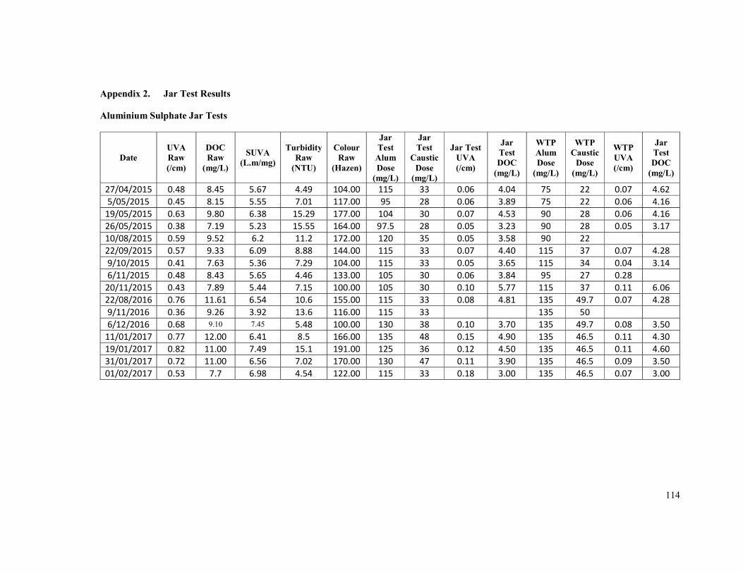
114

Appendix 2. Jar Test Results

Aluminium Sulphate Jar Tests

Date UVA Raw (/cm)

DOC Raw

(mg/L)

SUVA (L.m/mg)

Turbidity Raw

(NTU)

Colour Raw

(Hazen)

Jar Test

Alum Dose

(mg/L)

Jar Test

Caustic Dose

(mg/L)

Jar Test UVA (/cm)

Jar Test DOC

(mg/L)

WTP Alum Dose

(mg/L)

WTP Caustic

Dose (mg/L)

WTP UVA (/cm)

Jar Test DOC

(mg/L)

27/04/2015 0.48 8.45 5.67 4.49 104.00 115 33 0.06 4.04 75 22 0.07 4.62

5/05/2015 0.45 8.15 5.55 7.01 117.00 95 28 0.06 3.89 75 22 0.06 4.16

19/05/2015 0.63 9.80 6.38 15.29 177.00 104 30 0.07 4.53 90 28 0.06 4.16

26/05/2015 0.38 7.19 5.23 15.55 164.00 97.5 28 0.05 3.23 90 28 0.05 3.17

10/08/2015 0.59 9.52 6.2 11.2 172.00 120 35 0.05 3.58 90 22 22/09/2015 0.57 9.33 6.09 8.88 144.00 115 33 0.07 4.40 115 37 0.07 4.28

9/10/2015 0.41 7.63 5.36 7.29 104.00 115 33 0.05 3.65 115 34 0.04 3.14

6/11/2015 0.48 8.43 5.65 4.46 133.00 105 30 0.06 3.84 95 27 0.28

20/11/2015 0.43 7.89 5.44 7.15 100.00 105 30 0.10 5.77 115 37 0.11 6.06

22/08/2016 0.76 11.61 6.54 10.6 155.00 115 33 0.08 4.81 135 49.7 0.07 4.28

9/11/2016 0.36 9.26 3.92 13.6 116.00 115 33 135 50 6/12/2016 0.68 9.10 7.45 5.48 100.00 130 38 0.10 3.70 135 49.7 0.08 3.50

11/01/2017 0.77 12.00 6.41 8.5 166.00 135 48 0.15 4.90 135 46.5 0.11 4.30

19/01/2017 0.82 11.00 7.49 15.1 191.00 125 36 0.12 4.50 135 46.5 0.11 4.60

31/01/2017 0.72 11.00 6.56 7.02 170.00 130 47 0.11 3.90 135 46.5 0.09 3.50

01/02/2017 0.53 7.7 6.98 4.54 122.00 115 33 0.18 3.00 135 46.5 0.07 3.00

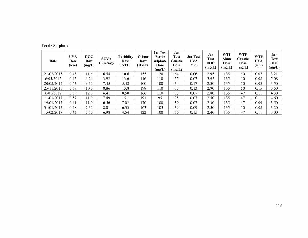
115

Ferric Sulphate

Date UVA Raw (/cm)

DOC Raw

(mg/L)

SUVA (L.m/mg)

Turbidity Raw

(NTU)

Colour Raw

(Hazen)

Jar Test Ferric

sulphate Dose

(mg/L)

Jar Test

Caustic Dose

(mg/L)

Jar Test UVA (/cm)

Jar Test DOC

(mg/L)

WTP Alum Dose

(mg/L)

WTP Caustic

Dose (mg/L)

WTP UVA (/cm)

Jar Test DOC

(mg/L)

21/02/2015 0.48 11.6 6.54 10.6 155 120 64 0.06 2.95 135 50 0.07 3.21 6/05/2015 0.45 9.26 3.92 13.6 116 110 57 0.07 3.95 135 50 0.08 5.08 20/05/2015 0.63 9.10 7.45 5.48 100 100 34 0.17 2.30 135 50 0.08 3.50 25/11/2016 0.38 10.0 8.86 13.8 198 110 33 0.13 2.90 135 50 0.15 5.50 6/01/2017 0.59 12.0 6.41 8.50 166 110 33 0.07 2.80 135 47 0.11 4.30 11/01/2017 0.57 11.0 7.49 15.1 191 95 28 0.07 2.50 135 47 0.11 4.60 19/01/2017 0.41 11.0 6.56 7.02 170 100 30 0.07 2.30 135 47 0.09 3.50 31/01/2017 0.48 7.30 8.01 6.33 163 105 36 0.09 2.50 135 50 0.08 3.20 15/02/2017 0.43 7.70 6.98 4.54 122 100 30 0.15 2.40 135 47 0.11 3.00

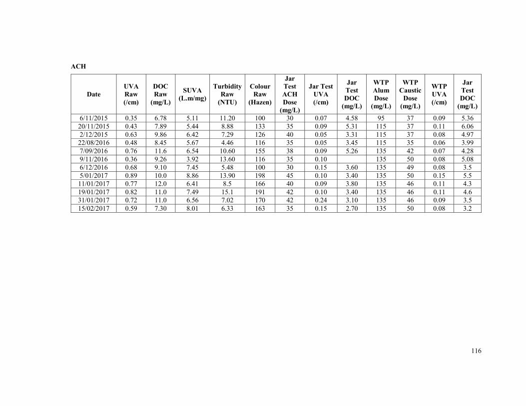
116

ACH

Date UVA Raw (/cm)

DOC Raw

(mg/L)

SUVA (L.m/mg)

Turbidity Raw

(NTU)

Colour Raw

(Hazen)

Jar Test ACH Dose

(mg/L)

Jar Test UVA (/cm)

Jar Test DOC

(mg/L)

WTP Alum Dose

(mg/L)

WTP Caustic

Dose (mg/L)

WTP UVA (/cm)

Jar Test DOC

(mg/L)

6/11/2015 0.35 6.78 5.11 11.20 100 30 0.07 4.58 95 37 0.09 5.36 20/11/2015 0.43 7.89 5.44 8.88 133 35 0.09 5.31 115 37 0.11 6.06 2/12/2015 0.63 9.86 6.42 7.29 126 40 0.05 3.31 115 37 0.08 4.97 22/08/2016 0.48 8.45 5.67 4.46 116 35 0.05 3.45 115 35 0.06 3.99 7/09/2016 0.76 11.6 6.54 10.60 155 38 0.09 5.26 135 42 0.07 4.28 9/11/2016 0.36 9.26 3.92 13.60 116 35 0.10 135 50 0.08 5.08 6/12/2016 0.68 9.10 7.45 5.48 100 30 0.15 3.60 135 49 0.08 3.5 5/01/2017 0.89 10.0 8.86 13.90 198 45 0.10 3.40 135 50 0.15 5.5 11/01/2017 0.77 12.0 6.41 8.5 166 40 0.09 3.80 135 46 0.11 4.3 19/01/2017 0.82 11.0 7.49 15.1 191 42 0.10 3.40 135 46 0.11 4.6 31/01/2017 0.72 11.0 6.56 7.02 170 42 0.24 3.10 135 46 0.09 3.5 15/02/2017 0.59 7.30 8.01 6.33 163 35 0.15 2.70 135 50 0.08 3.2

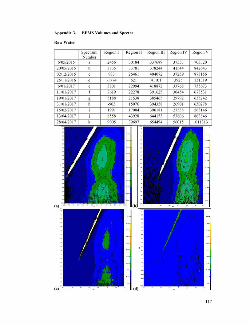
117

Appendix 3. EEMS Volumes and Spectra

Raw Water

Spectrum Number

Region I Region II Region III Region IV Region V

6/05/2015 a 2456 30184 337689 37553 703320

20/05/2015 b 3835 33781 378244 41544 842643

02/12/2015 c 933 26461 404072 37259 873156

25/11/2016 d -1774 621 41101 3925 131319

6/01/2017 e 3801 22994 418872 33768 735673

11/01/2017 f 7619 22278 391625 30454 673531

19/01/2017 g 5188 21538 385465 29792 635242

31/01/2017 h -903 15076 394358 26901 630278

15/02/2017 i 1991 17004 390181 27538 563146

13/04/2017 j 8558 43928 644153 53806 863846

28/04/2017 k 9005 39697 654494 56015 1011313

(a) (b)

(c) (d)

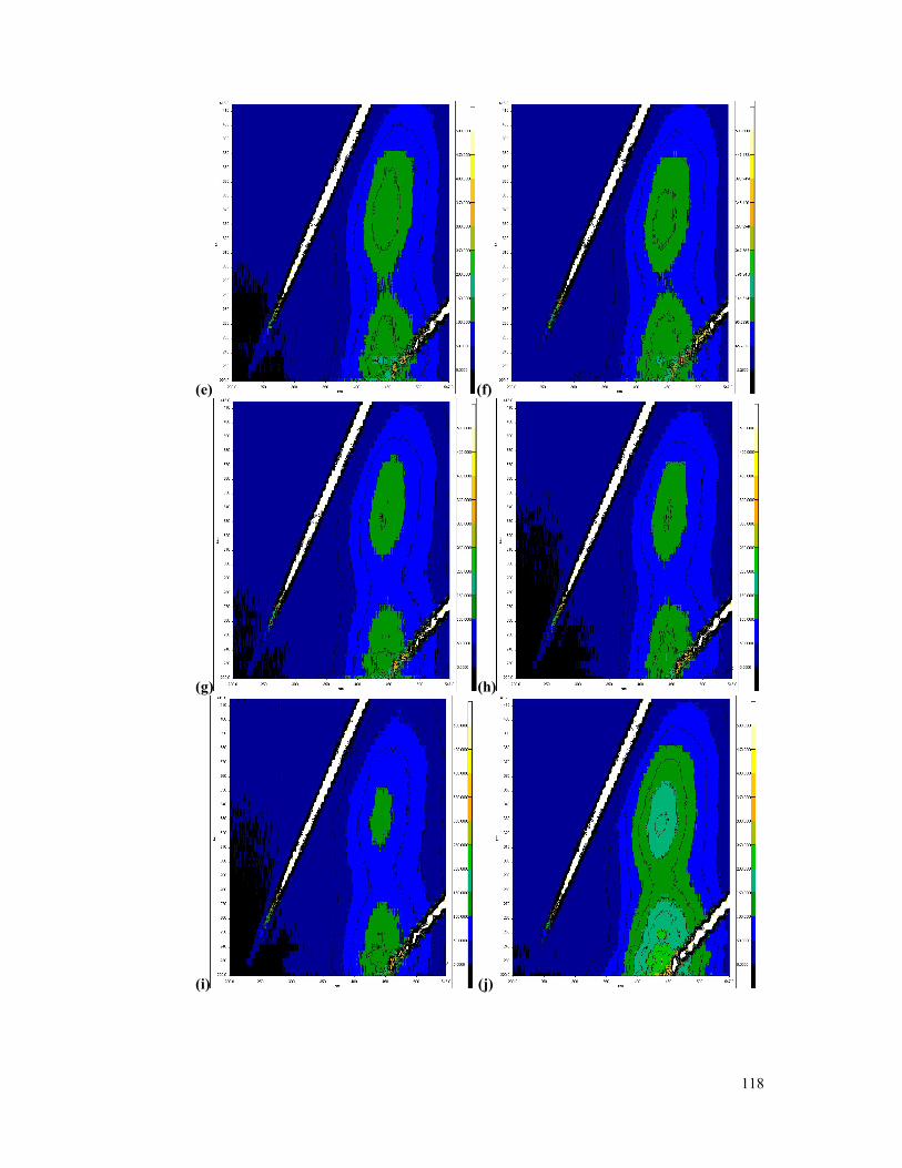
118

(e) (f)

(g) (h)

(i) (j)

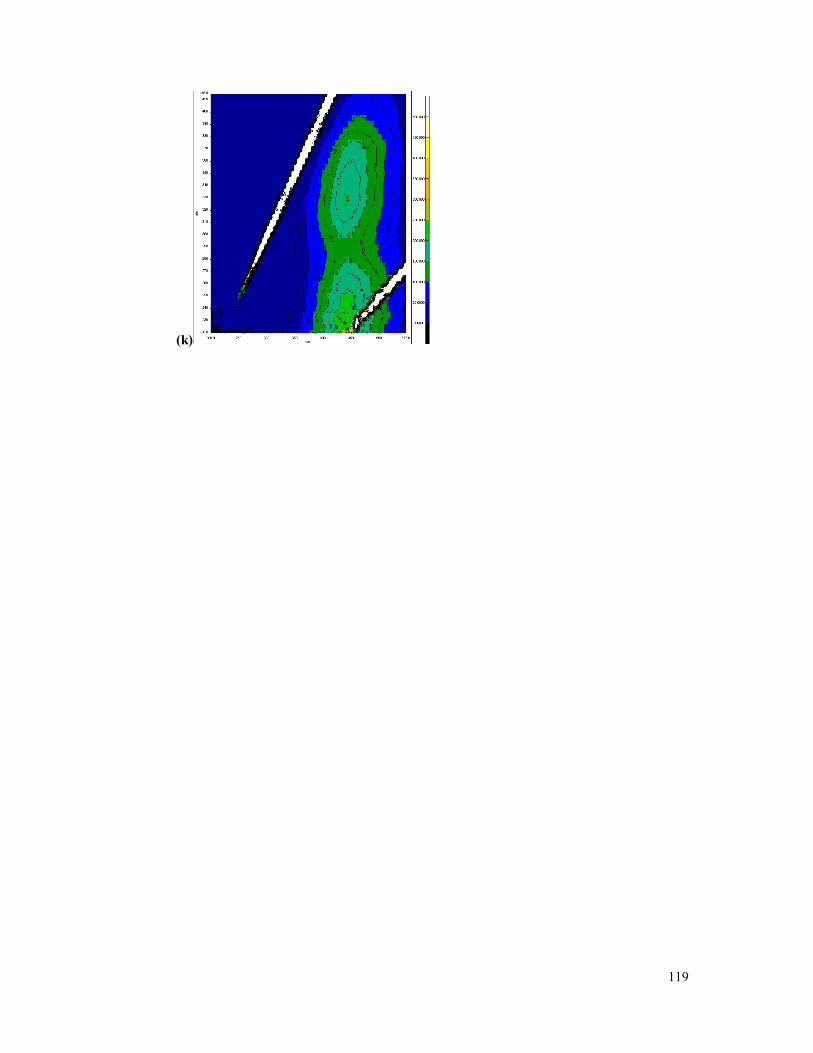
119

(k)

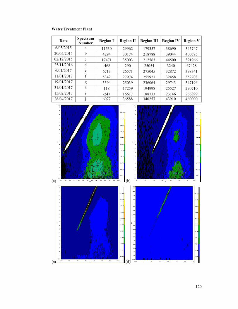
120

Water Treatment Plant

Date Spectrum Number

Region I Region II Region III Region IV Region V

6/05/2015 a 11530 29962 179357 38690 345747 20/05/2015 b 4294 30174 218788 39044 400595 02/12/2015 c 17471 35003 212563 44500 391966 25/11/2016 d -468 290 25054 3240 67428 6/01/2017 e 6713 26571 275045 32872 398341 11/01/2017 f 5342 27974 255921 32458 352708 19/01/2017 g 3594 25039 236064 29743 347196 31/01/2017 h 118 17259 194998 25527 290710 15/02/2017 i -247 16617 188733 23146 266899 28/04/2017 j 6077 36588 340257 43910 460000

(a) (b)

(c) (d)

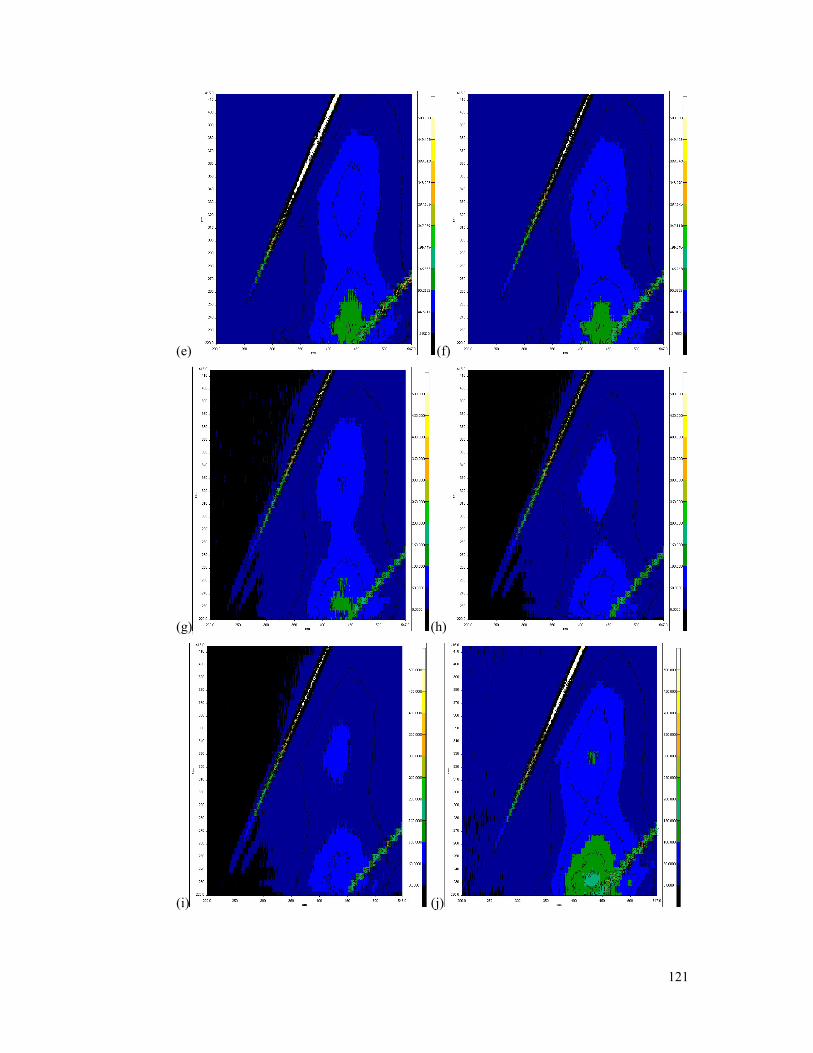
121

(e) (f)

(g) (h)

(i) (j)

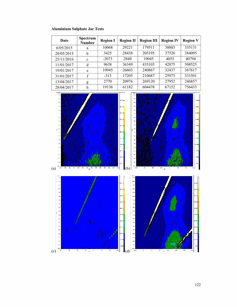
122

Aluminium Sulphate Jar Tests

Date Spectrum Number

Region I Region II Region III Region IV Region V

6/05/2015 a 10068 29221 179511 38883 335131

20/05/2015 b 3425 28438 205195 37526 384095

25/11/2016 c -2073 2849 19045 4055 40794

11/01/2017 d 9638 36349 435103 42875 508525

19/01/2017 e 10945 26603 240867 32437 367617

31/01/2017 f -313 17205 210687 25973 331501

13/04/2017 g 2770 20976 269120 27952 246857

28/04/2017 h 19136 61182 604478 67152 756433

(a) (b)

(c) (d)

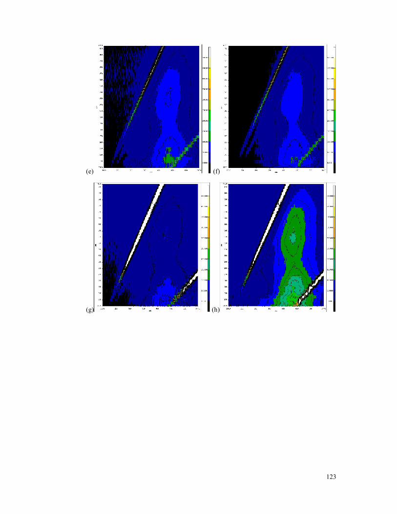
123

(e) (f)

(g) (h)

124

Ferric Sulphate Jar Tests

Date Spectrum Number

Region I Region II Region III Region IV Region V

25/11/2016 a -533 860 19069 1216 38970

6/01/2017 b 10215 27421 186532 29163 245312

11/01/2017 c 7703 19169 146505 22817 188078

19/01/2017 d 758 16707 147490 21474 190668

31/01/2017 e -594 9871 111994 16491 149702

15/02/2017 f 1164 15936 163655 21526 215285

13/04/2017 g 1316 13587 124862 18291 140304

28/04/2017 h 5639 23968 356491 32960 263849

(a) (b)

(c) (d)

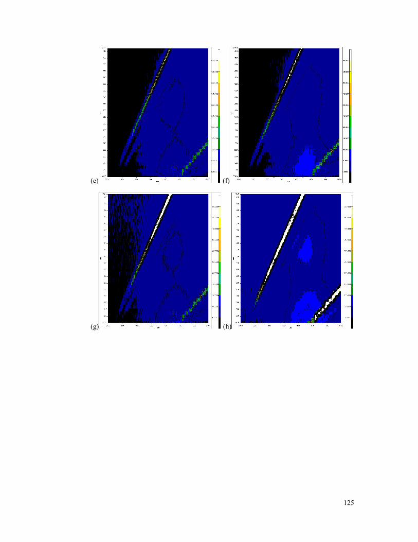
125

(e) (f)

(g) (h)

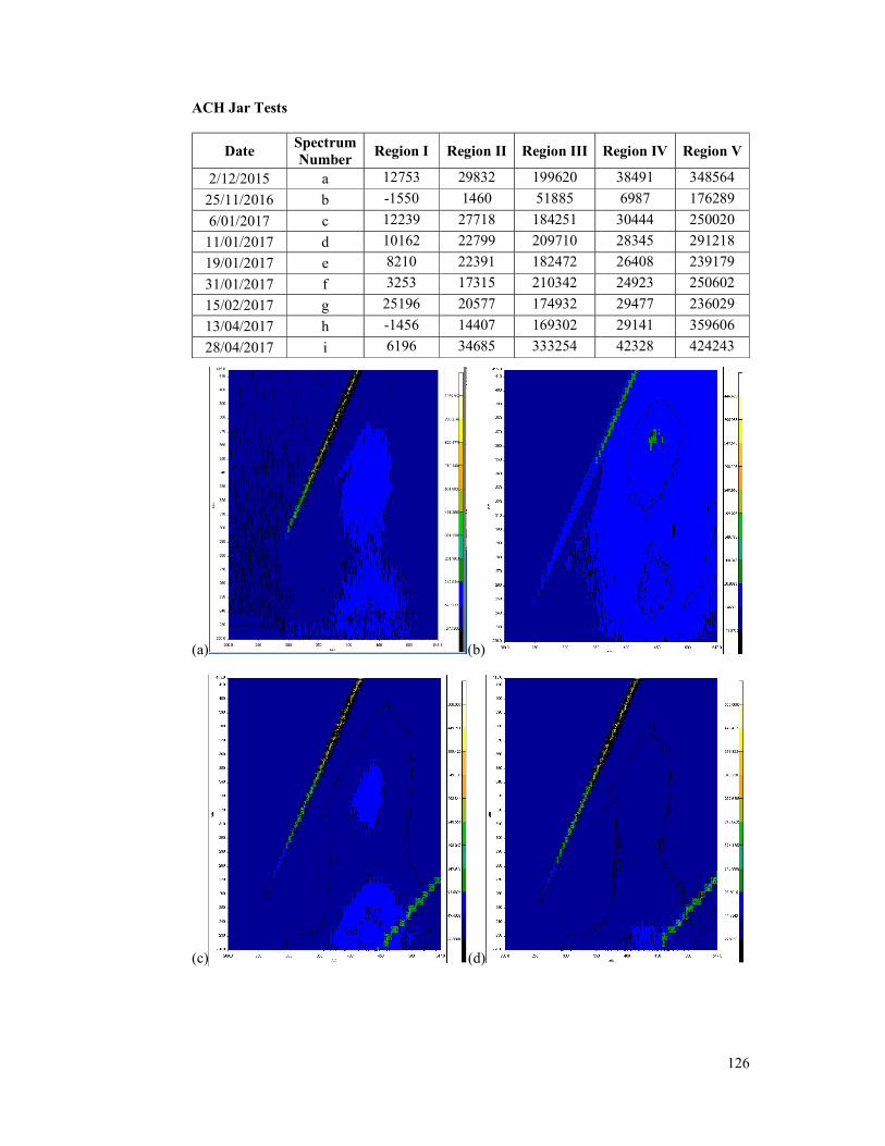
126

ACH Jar Tests

Date Spectrum Number

Region I Region II Region III Region IV Region V

2/12/2015 a 12753 29832 199620 38491 348564

25/11/2016 b -1550 1460 51885 6987 176289

6/01/2017 c 12239 27718 184251 30444 250020

11/01/2017 d 10162 22799 209710 28345 291218

19/01/2017 e 8210 22391 182472 26408 239179

31/01/2017 f 3253 17315 210342 24923 250602

15/02/2017 g 25196 20577 174932 29477 236029

13/04/2017 h -1456 14407 169302 29141 359606

28/04/2017 i 6196 34685 333254 42328 424243

(a) (b)

(c) ( (d)

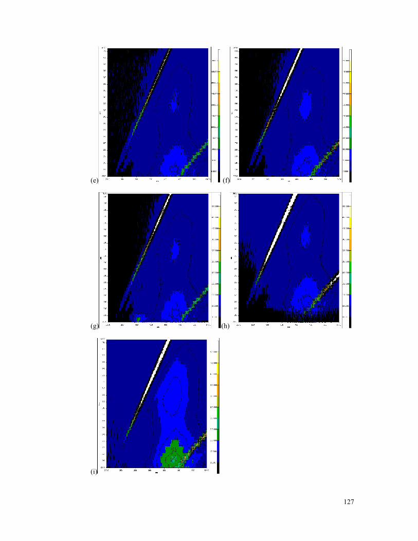
127

(e) (f)

(g) (h)

(i)

128

Appendix 4. DOC fractions associated with Liquid Chromatography Organic Carbon

Detection

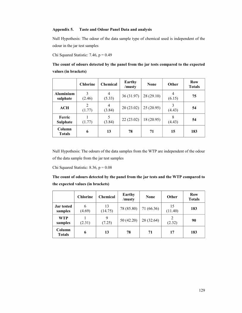
129

Appendix 5. Taste and Odour Panel Data and analysis

Null Hypothesis: The odour of the data sample type of chemical used is independent of the

odour in the jar test samples

Chi Squared Statistic: 7.46, p = 0.49

The count of odours detected by the panel from the jar tests compared to the expected

values (in brackets)

Chlorine Chemical Earthy /musty

None Other Row

Totals

Aluminium sulphate

3 (2.46)

4 (5.33)

36 (31.97) 28 (29.10) 4

(6.15) 75

ACH 2

(1.77) 4

(3.84) 20 (23.02) 25 (20.95)

3 (4.43) 54

Ferric Sulphate

1 (1.77)

5 (3.84)

22 (23.02) 18 (20.95) 8

(4.43) 54

Column Totals

6 13 78 71 15 183

Null Hypothesis: The odours of the data samples from the WTP are independent of the odour

of the data sample from the jar test samples

Chi Squared Statistic: 8.36, p = 0.08

The count of odours detected by the panel from the jar tests and the WTP compared to

the expected values (in brackets)

Chlorine Chemical Earthy /musty

None Other Row

Totals

Jar tested samples

6 (4.69)

13 (14.75)

78 (85.80) 71 (66.36) 15

(11.40) 183

WTP samples

1 (2.31)

9 (7.25)

50 (42.20) 28 (32.64) 2

(2.32) 90

Column Totals

6 13 78 71 17 183

130

Null Hypothesis: The odours of the data samples from the final water samples (Euroa and

Shepparton) are independent of the odour of the data sample from the jar test samples

Chi Squared Statistic: 182.41, p < 0.00001

The count of odours detected by the panel from the jar tests, the WTP, and the final

water from Shepparton and Euroa compared to the expected values (in brackets)

Chlorine Chemical Earthy /musty

None Other Row

Totals

Jar tests 6

(30.08) 13 (16.94) 78 (70.32) 71 (55.92) 15 (9.74) 183

WTP 1 (14.79 9 (8.33) 50 (34.58) 28 (27.50) 2 (4.79) 90

Euroa final 14 (13.15) 10 (7.41) 31 (30.74) 20 (24.44) 5 (4.26) 80

Shepparton 50 (12.98) 8 (7.31) 7 (30.36) 13 (24.14) 1 (4.21) 79

Column Totals

71 40 166 132 23 432

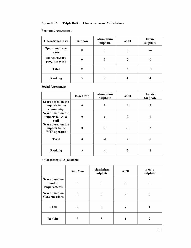
131

Appendix 6. Triple Bottom Line Assessment Calculations

Economic Assessment

Operational costs Base case Aluminium

sulphate ACH

Ferric sulphate

Operational cost score

0 1 3 -4

Infrastructure program score

0 0 2 0

Total 0 1 5 -4

Ranking 3 2 1 4

Social Assessment

Base Case Aluminium

Sulphate ACH

Ferric Sulphate

Score based on the impacts to the

community 0 0 3 2

Score based on the impacts to GVW

staff 0 0 2 1

Score based on the impacts to the WTP operator

0 -1 -1 3

Total 0 -1 4 6

Ranking 3 4 2 1

Environmental Assessment

Base Case Aluminium

Sulphate ACH

Ferric Sulphate

Score based on landfill

requirements 0 0 3 -1

Score based on CO2 emissions

0 0 4 2

Total 0 0 7 1

Ranking 3 3 1 2

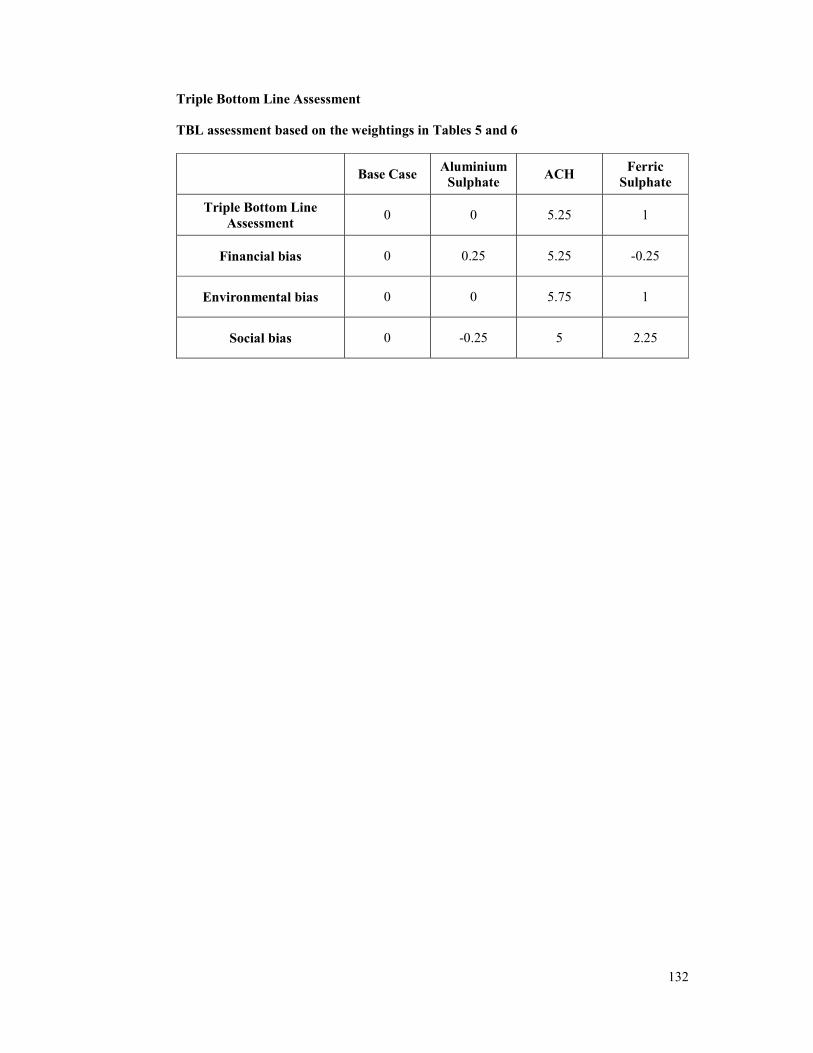
132

Triple Bottom Line Assessment

TBL assessment based on the weightings in Tables 5 and 6

Base Case Aluminium

Sulphate ACH

Ferric Sulphate

Triple Bottom Line Assessment

0 0 5.25 1

Financial bias 0 0.25 5.25 -0.25

Environmental bias 0 0 5.75 1

Social bias 0 -0.25 5 2.25