A birth and growth model for kinetic-driven crystallization processes, Part I: Modeling
22
Nonlinear Analysis: Real World Applications 10 (2009) 71–92 www.elsevier.com/locate/nonrwa A birth and growth model for kinetic-driven crystallization processes, Part I: Modeling Dino Aquilano a , Vincenzo Capasso b , Alessandra Micheletti b , Stefano Patti b,* , Livio Pizzocchero b , Marco Rubbo a a Dipartimento di Scienze Mineralogiche e Petrologiche, Universit` a di Torino, via Valperga Caluso 35, I-10125 Torino, Italy b Dipartimento di Matematica, Universit` a di Milano, Via C. Saldini 50, I-20133 Milano, Italy Received 7 August 2007; accepted 15 August 2007 Abstract We consider a birth and growth model for crystallization processes in d space dimensions, where growth is driven by the gradient of the concentration. A nonlinear condition for the concentration is given on the boundary and a multi-front moving boundary problem arises. We propose a new formulation based on the Schwartz distributions by coupling the growth of the crystals and the diffusion of the concentration. We complete the deterministic growth model by considering stochastic nucleations in space and time. The coupling of the growth dynamics with the evolution of the underlying field of the concentration of matter finally causes the stochastic geometry of the crystals. c 2007 Elsevier Ltd. All rights reserved. Keywords: Birth and growth processes; Crystal growth; Diffusion; Level set method 0. Introduction In this paper we propose a mathematical framework to analyze the evolution via nucleation and growth of population of crystals arising from an initially homogeneous phase. For technological purposes it is important to understand and master the process of mass crystallization, as well as to control the nucleation and growth of nano-sized particles. During crystallization the number, the shape and the size of crystals change with time, and peculiar textures are produced due to the interplay of kinetics and transport phenomena. In many situations direct interactions among crystals (producing agglomeration or breakage) do not occur and convective transport is negligible. For instance, this is the case of crystallization in gels, in steady magmatic fluids, in microgravity conditions. In these examples there is only a soft interaction between growing crystals, occurring when the volumes of solution from which they capture solute overlap. The depletion of solute around every crystal brings about diffusion in the solution. This is a process of multi-center diffusion due to the long range character of diffusion itself. The resulting crystallization patterns depend on the spatial distribution of crystals as determined by the stochastic nature of nucleation. In the final stage of the * Corresponding author. Tel.: +39 02 50316166; fax: +39 02 50316090. E-mail address: [email protected] (S. Patti). 1468-1218/$ - see front matter c 2007 Elsevier Ltd. All rights reserved. doi:10.1016/j.nonrwa.2007.08.015
Transcript of A birth and growth model for kinetic-driven crystallization processes, Part I: Modeling
Nonlinear Analysis: Real World Applications 10 (2009) 71–92www.elsevier.com/locate/nonrwa
A birth and growth model for kinetic-driven crystallizationprocesses, Part I: Modeling
Dino Aquilanoa, Vincenzo Capassob, Alessandra Michelettib, Stefano Pattib,∗,Livio Pizzoccherob, Marco Rubboa
a Dipartimento di Scienze Mineralogiche e Petrologiche, Universita di Torino, via Valperga Caluso 35, I-10125 Torino, Italyb Dipartimento di Matematica, Universita di Milano, Via C. Saldini 50, I-20133 Milano, Italy
Received 7 August 2007; accepted 15 August 2007
Abstract
We consider a birth and growth model for crystallization processes in d space dimensions, where growth is driven by thegradient of the concentration. A nonlinear condition for the concentration is given on the boundary and a multi-front movingboundary problem arises. We propose a new formulation based on the Schwartz distributions by coupling the growth of the crystalsand the diffusion of the concentration. We complete the deterministic growth model by considering stochastic nucleations in spaceand time. The coupling of the growth dynamics with the evolution of the underlying field of the concentration of matter finallycauses the stochastic geometry of the crystals.c© 2007 Elsevier Ltd. All rights reserved.
Keywords: Birth and growth processes; Crystal growth; Diffusion; Level set method
0. Introduction
In this paper we propose a mathematical framework to analyze the evolution via nucleation and growth ofpopulation of crystals arising from an initially homogeneous phase. For technological purposes it is important tounderstand and master the process of mass crystallization, as well as to control the nucleation and growth of nano-sizedparticles. During crystallization the number, the shape and the size of crystals change with time, and peculiar texturesare produced due to the interplay of kinetics and transport phenomena. In many situations direct interactions amongcrystals (producing agglomeration or breakage) do not occur and convective transport is negligible. For instance, thisis the case of crystallization in gels, in steady magmatic fluids, in microgravity conditions. In these examples thereis only a soft interaction between growing crystals, occurring when the volumes of solution from which they capturesolute overlap. The depletion of solute around every crystal brings about diffusion in the solution. This is a process ofmulti-center diffusion due to the long range character of diffusion itself. The resulting crystallization patterns dependon the spatial distribution of crystals as determined by the stochastic nature of nucleation. In the final stage of the
∗ Corresponding author. Tel.: +39 02 50316166; fax: +39 02 50316090.E-mail address: [email protected] (S. Patti).
1468-1218/$ - see front matter c© 2007 Elsevier Ltd. All rights reserved.doi:10.1016/j.nonrwa.2007.08.015
72 D. Aquilano et al. / Nonlinear Analysis: Real World Applications 10 (2009) 71–92
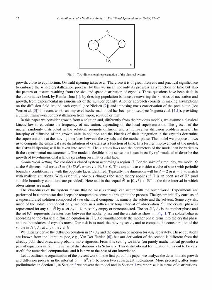
Fig. 1. Two-dimensional representation of the physical system.
growth, close to equilibrium, Ostwald ripening takes over. Therefore it is of great theoretic and practical significanceto embrace the whole crystallization process: by this we mean not only its progress as a function of time but alsothe pattern or texture resulting from the size and space distribution of crystals. These questions have been dealt inthe authoritative book by Ramkrishna [1], by dressing population balances, recovering the kinetics of nucleation andgrowth, from experimental measurements of the number density. Another approach consists in making assumptionson the diffusion field around each crystal (see Nielsen [2]) and imposing mass conservation of the precipitate (seeWert et al. [3]). In recent works an improved isothermal model has been proposed (see Noguera et al. [4,5]), providinga unified framework for crystallization from vapor, solution or melt.
In this paper we consider growth from a solution and, differently from the previous models, we assume a classicalkinetic law to calculate the frequency of nucleation, depending on the local supersaturation. The growth of thenuclei, randomly distributed in the solution, promote diffusion and a multi-center diffusion problem arises. Theinterplay of diffusion of the growth units in solution and the kinetics of their integration in the crystals determinethe supersaturation at the moving interfaces between the crystals and the mother phase. The model we propose allowsus to compute the empirical size distribution of crystals as a function of time. In a further improvement of the model,the Ostwald ripening will be taken into account. The kinetics laws and the parameters of the model can be varied tofit the experimental measurements. The model is flexible in the sense that it can be easily reformulated to describe thegrowth of two-dimensional islands spreading on a flat crystal face.
Geometrical Setting. We consider a closed system occupying a region Ω . For the sake of simplicity, we model Ωas the d-dimensional torus Ω = (R/ lZ)d , where l ∈ R, l > 0. This amounts to consider a cube of size l with periodicboundary conditions, i.e. with the opposite faces identified. Typically, the dimension will be d = 2 or d = 3, to matchwith realistic situations. With essentially obvious changes the same theory applies if Ω is an open set of Rd (andsuitable boundary conditions are provided). Here and in the sequel Θ = [0, t f ) ⊂ R+ is the time interval in whichobservations are made.
The closedness of the system means that no mass exchange can occur with the outer world. Experiments areperformed in a thermostat that keeps the temperature constant throughout the process. The system initially consists ofa supersaturated solution composed of two chemical components, namely the solute and the solvent. Some crystals,made of the solute component only, are born in a sufficiently long interval of observation Θ . The crystal phase isrepresented for any t ∈ Θ by a set At ⊂ Ω , possibly empty or nonconnected. The set Ω \ At is the mother phase andthe set ∂At represents the interfaces between the mother phase and the crystals as shown in Fig. 1. The solute behavesaccording to the classical diffusion equation in Ω \ At ; simultaneously the mother phase turns into the crystal phaseand the boundaries of crystals move. Our task is to track the moving set At and to compute the concentration of thesolute in Ω \ At at any time t ∈ Θ .
We initially derive the diffusion equation in Ω \ At and the equation of motion for ∂At separately. These equationsare known from the literature (see, e.g., Van Der Eerden [6]) but our derivation of the second is different from thealready published ones, and probably more rigorous. From this setting we infer (on purely mathematical grounds) apair of equations in Ω in the sense of distributions a la Schwartz. This distributional formulation turns out to be veryuseful for numerical computations and it is new to the best of our knowledge.
Let us outline the organization of the present work. In the first part of the paper, we analyze the deterministic growthand diffusion process in the interval Θ = [t0, t1) between two subsequent nucleations. More precisely, after somepreliminaries in Section 1, in Section 2 we present the model and in Section 3 we rephrase it in terms of distributions.

D. Aquilano et al. / Nonlinear Analysis: Real World Applications 10 (2009) 71–92 73
The second part of the paper, starting from Section 4, deals with multiple births occurring stochastically at differenttimes. In Section 4 we propose a nucleation model based on a space–time point process and we give a short accounton the geometry of the critical nuclei. In Section 5 we merge the equations derived so far in a unique birth and growthmodel, and in Section 6 we present some numerical results.
1. Some notations and preliminaries
We now give some basic definitions and results that will be used throughout the paper. We denote with B(Ω) ≡ Bthe Borel σ -algebra of the torus Ω . For each σ ∈ R+, Hσ is the σ -dimensional Hausdorff measure on Ω . Whenrestricted, say, to B, the measureHd will be called as usually the Lebesgue measure; in integrals we will simply writedx for Hd(dx). For any open set B ⊂ Ω , ∂B denotes its boundary and we write ∂1 B for the C1 part of ∂B (see,e.g., Giaquinta et al. [7]).
Definition 1.1. A set B ⊂ Ω is regular if B is open, ∂B has Hausdorff dimension d − 1 and Hd−1(∂B \ ∂1 B) = 0(i.e., ∂B is almost everywhere C1). We will denote byReg(Ω), or simplyReg, the regular subsets of Ω .
For B ∈ Reg, the outward normal unit vector to the boundary is defined and continuous on ∂1 B (i.e. almosteverywhere on ∂B).
In the sequel, we often consider a real interval of the form Θ = [t0, t1). Given such an interval, for t ∈ Θ andς > 0, we put I (t, ς) := (t − ς, t + ς) ∩ Θ .
Definition 1.2. A regular time-dependent set is a family B = (Bt )t∈Θ s.t.
(i) Bt ∈ Reg, ∀t ∈ Θ ;(ii) for any t ∈ Θ there exist ς > 0, and a family of maps (φt ′,t )t ′∈I , t ′ ∈ I (t, ς) s.t.:
– ∀t ′ ∈ I (t, ς), φt ′,t : Ω → Ω is a C1 diffeomorphism of the torus into itself;– the map I (t, ς)× Ω → Ω , (t ′, x) 7→ φt ′,t (x) is C1;– φt,t = idΩ and φt ′,t (Bt ) = Bt ′ , ∀t ′ ∈ I (t, ς).
Given such a family, we will put
KB :=
⋃t∈(t0,t1)
Bt × t KB :=
⋃t∈[t0,t1)
Bt × t; Ω \ B := (Ω \ Bt )t∈Θ .
(Bt denoting the closure of the set Bt ; Ω \ B is also a regular time-dependent set).
Remark 1.3. (i) The conditions in Definition 1.2 imply the following: ∀t ∈ Θ , ∀s ∈ ∂1 Bt , there are ε, ς > 0, a localCartesian coordinate system y : U ⊆ Ω → (−ε, ε)d (with U an open neighborhood of s) and a C1 function
F : (−ε, ε)d−1× I (t, ς) −→ (−ε/2, ε/2)
(y1, . . . , yd−1, t ′) 7−→ F(y1, . . . , yd−1, t ′)
s.t. ∀t ′ ∈ I (t, ς), y(Bt ′ ∩U) = y ∈ (−ε, ε)d : yd < F(y1, . . . , yd−1, t ′) and y(∂Bt ′ ∩U) = y ∈ (−ε, ε)d : yd =
F(y1, . . . , yd−1, t ′).(ii) One can prove the following:KB is an open subset of Ω ×(−∞, t1) (with the product topology);KB is its closure
in this topological space.
Definition 1.4. Let B = (Bt )t∈Θ be a regular time-dependent set. The normal speed at time t is the function
w(·, t) : ∂1 Bt → R, s 7→ w(s, t) := w(s, t) · m(s, t),
where m(s, t) is the outward normal unit vector to ∂Bt at s and
w(s, t) :=∂
∂t
∣∣∣∣t ′=t
φt ′,t (s); (1.1)
here (φt ′,t )t ′∈I (t,ς) is any family of diffeomorphisms as in Definition 1.2. The normal speed w(s, t) = w(s, t) · m(s, t)is independent of the choice of φt ′,t , see Appendix.
74 D. Aquilano et al. / Nonlinear Analysis: Real World Applications 10 (2009) 71–92
Of course, the outward normal unit vector and the normal speed for the family Ω \ B are −m(s, t), −w(s, t). Forsubsequent reference, let us write down some classical integral identities (see, e.g., Giaquinta et al. [7] and Miranvilleet al. [8], Prop. 4, p. 18).
Theorem 1.5 (Gauss Theorem). Let B ∈ Reg and let m = (m1, . . . ,md) be the outward normal unit vector to ∂B.Let f ∈ C1(B,R). Then∫
B
∂ f
∂xi(x)dx =
∫∂B
f (s)mi (s)ds, (1.2)
here and in the sequel, ds is a short-hand notations for Hd−1(ds).
A corollary of the Gauss Theorem is the following Divergence Theorem. Let f ∈ C1(B,Rd), with B and m as before.Then ∫
B∇ · f(x)dx =
∫∂B
f(s) · m(s)ds. (1.3)
Theorem 1.6 (Reynolds Transport Theorem). Let (Bt )t∈Θ be a regular time-dependent set, moving with normalspeed w and let f ∈ C1(KB,R). Then the function t ∈ Θ 7→
∫Bt
f (x, t)dx is C1 and, for all t ∈ Θ ,
ddt
∫Bt
f (x, t)dx =
∫Bt
∂ f
∂t(x, t)dx +
∫∂Bt
f (s, t)w(s, t)ds. (1.4)
2. Derivation of growth and diffusion equations
Crystallization processes have been intensively modeled by physicists and mathematicians as moving boundaryproblems, where the growth depends linearly on the temperature or concentration gradient: see, e.g., Burger et al. [9,10], Capasso et al. [11], Colli et al. [12] or Rubbo [13]. Here we propose a new model, supported by empiricalevidence, where heat fluxes and volume variations of the system are neglected; hence the crystallization process isonly driven by a gradient of the concentration of matter constituting the mono-component crystal phase. Differentlyfrom the classical Stefan problems, we will show that a nonlinear condition for the concentration holds on the movingboundary.
2.1. Initial assumptions
As explained in the introduction, the aim of this section is to model the deterministic process of growth anddiffusion between two subsequent crystal nucleations, occurring at two instants t0 and t1. Let
Θ := [t0, t1) ⊂ R+; (2.1)
during this interval there are no nucleations, so the crystals can only grow. We assume that crystals do not coalesce;this idea will be formalized as follows.
Definition 2.1. For each t ∈ Θ , At ⊂ Ω is the region occupied by crystals at time t ; so Ω \ At represents the motherphase.
Assumption 2.2 (On the Crystals).
(i) (At )t∈Θ is a regular time-dependent set, so we can define the outward normal unit vector n to ∂At and the normalspeed v(·, t).
(ii) For each t ∈ Θ , At has finitely many connected components Aht ∈ Reg (h ∈ H ), where Ah
t represents the hthcrystal grown up to time t (so, At =
⋃h∈H Ah
t and Aht0 ∩ Ah′
t0 = ∅ for h, h′∈ H , h 6= h′). In particular Ah
t0 are
the crystals existing at time t0; i.e., the ones born and grown up to t0.
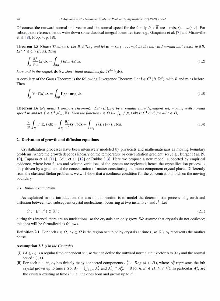
D. Aquilano et al. / Nonlinear Analysis: Real World Applications 10 (2009) 71–92 75
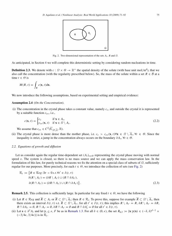
Fig. 2. Two-dimensional representation of the sets At , R and Ω .
As anticipated, in Section 4 we will complete this deterministic setting by considering random nucleations in time.
Definition 2.3. We denote with c : Ω × Θ → R+ the spatial density of the solute (with base unit mol/md), that wealso call the concentration (with the regularity prescribed below). So, the mass of the solute within a set R ∈ B at atime t ∈ Θ is
M(R, t) =
∫R
c(x, t)dx.
We now introduce the following assumptions, based on experimental setting and empirical evidence:
Assumption 2.4 (On the Concentration).
(i) The concentration in the crystal phase takes a constant value, namely cs , and outside the crystal it is representedby a suitable function cex , i.e.,
c(x, t) =
cs if x ∈ At ,
cex (x, t) if x ∈ Ω \ At .(2.2)
We assume that cex ∈ C2(KΩ\A,R).(ii) The crystal phase is more dense than the mother phase, i.e. cs > cex (x, t)∀x ∈ Ω \ At ,∀t ∈ Θ . Since the
inequality is strict, a jump in the concentration always occurs on the boundary ∂At , ∀t ∈ Θ .
2.2. Equations of growth and diffusion
Let us consider again the regular time-dependent set (At )t∈Θ representing the crystal phase moving with normalspeed v. The system is closed, so there is no mass source and we can apply the mass conservation law. In theformulation of this law, for purely technical reasons we fix the attention on a special class of subsets of Ω , sufficientlyregular for our purposes. More precisely, for each t ∈ Θ , we introduce the collection of sets (see Fig. 2)
Rt :=
R ∈ Reg: ∃τ > 0 s.t.∀t ′ ∈ I (t, τ )
∂(R \ At ′) = (∂R \ At ′) ∪ (R ∩ ∂At ′),
∂(R ∩ At ′) = (∂R ∩ At ′) ∪ (R ∩ ∂At ′). (2.3)
Remark 2.5. This collection is sufficiently large. In particular for any fixed t ∈ Θ , we have the following
(i) Let R ∈ Reg and R ⊂ At or R ⊂ Ω \ At ; then R ∈ Rt . To prove this, suppose for example R ⊂ Ω \ At , thenthere exists an interval I (t, τ ) s.t. R ⊂ Ω \ At ′ , for all t ′ ∈ I (t, τ ); this implies R \ At ′ = R, ∂R \ At ′ = ∂R,R ∩ ∂At ′ = ∅, R ∩ At ′ = ∅, ∂R ∩ At ′ = ∅ and R ∩ ∂A′
t = ∅ for all t ′ ∈ I (t, τ ).(ii) Let s ∈ ∂1 At and let y, ς, ε, F be as in Remark 1.3. For all δ ∈ (0, ε), the set Rs,δ := x: y(x) ∈ (−δ, δ)d−1
×
(−3/4ε, 3/4ε) is inRt .
76 D. Aquilano et al. / Nonlinear Analysis: Real World Applications 10 (2009) 71–92
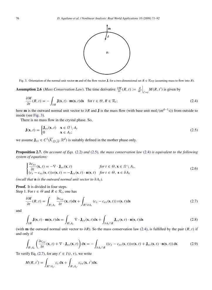
Fig. 3. Orientation of the normal unit vector m and of the flow vector J, for a two-dimensional set R ∈ Reg (assuming mass to flow into R).
Assumption 2.6 (Mass Conservation Law). The time derivative ∂M∂t (R, t) :=
ddt ′
∣∣∣t ′=t
M(R, t ′) is given by
∂M
∂t(R, t) = −
∫∂R
J(s, t) · m(s, t)ds for t ∈ Θ, R ∈ Rt ; (2.4)
here m is the outward normal unit vector to ∂R and J is the mass flow (with base unit mol/(md−1s)) from outside toinside (see Fig. 3).
There is no mass flow in the crystal phase. So,
J(x, t) =
Jex (x, t) x ∈ Ω \ At0 x ∈ At ;
(2.5)
we assume Jex ∈ C1(KΩ\A,Rd) is suitably defined in the mother phase only.
Proposition 2.7. On account of Eqs. (2.2) and (2.5), the mass conservation law (2.4) is equivalent to the followingsystem of equations:
∂cex
∂t(x, t) = −∇ · Jex (x, t) for t ∈ Θ, x ∈ Ω \ At ,
(cs − cex (s, t))v(s, t) = −Jex (s, t) · n(s, t) for t ∈ Θ, s ∈ ∂At
(2.6)
(recall that n is the outward normal unit vector to ∂At ).
Proof. It is divided in four steps.Step 1. For t ∈ Θ and R ∈ Rt , one has
∂M
∂t(R, t) =
∫R\At
∂cex
∂t(x, t)dx +
∫R∩∂At
(cs − cex (s, t)) v(s, t)ds (2.7)
and ∫∂R
J(s, t) · m(s, t)ds =
∫R\At
∇ · Jex (x, t)dx +
∫∂At ∩R
Jex (s, t) · n(s, t)ds (2.8)
(with m the outward normal unit vector to ∂R). So the mass conservation law (2.4), is fulfilled by the pair (R, t) ifand only if∫
R\At
(∂cex
∂t(x, t)+ ∇ · Jex (x, t)
)dx = −
∫∂At ∩R
((cs − cex (s, t))v(s, t)+ Jex (s, t) · n(s, t)) ds. (2.9)
To verify Eq. (2.7), for any t ′ ∈ I (t, τ ), we write
M(R, t ′) =
∫R∩At ′
cs dx +
∫R\At ′
cex (x, t ′)dx.
D. Aquilano et al. / Nonlinear Analysis: Real World Applications 10 (2009) 71–92 77
Hence
ddt ′
M(R, t ′) =d
dt ′
∫R∩At ′
cs dx +d
dt ′
∫R\At ′
cex (x, t ′)dx. (2.10)
The boundary ∂(R ∩ At ′) is the disjoint union of the sets (∂R ∩ At ′) and (R ∩ ∂At ′). In particular (R ∩ ∂At ′) ⊂ ∂At ′
and here the normal speed is a.e. equal to the function v(·, t ′) given in Assumption 2.2. Finally, (∂R ∩ At ′) ⊂ ∂Rthen, since R is time independent, its normal speed is equal to zero.
We now apply the Reynolds Transport Theorem (Eq. (1.4)) with Bt ′ := R ∩ At ′ and f (x, t ′) := cs ; this gives
ddt ′
∫R∩At ′
cs dx =
∫R∩∂At ′
csv(s, t ′)ds. (2.11)
We apply again the Reynolds Transport Theorem now taking Bt ′ := R \ At ′ and f (x, t ′) := cex (x, t ′) (Note that theintegration of cex on R \ At ′ or R \ At ′ gives the same result). We can write ∂(R \ At ′) as the union of two disjointsets, namely (∂R \ At ′) and (R ∩ ∂At ′). The normal speed on ∂R \ At ′ is zero; on R ∩ ∂At ′ the normal unit vector isthe opposite of the normal unit vector n to ∂At ′ and the normal speed is −v(·, t ′) (up to sets of zero measure).
ddt ′
∫R\At ′
cex (x, t ′)dx =
∫R\At ′
∂cex
∂t ′(x, t ′)dx −
∫R∩∂At ′
cex (s, t ′)v(s, t ′)ds. (2.12)
We substitute Eqs. (2.11) and (2.12) in Eq. (2.10), this gives,
ddt ′
M(R, t ′) =
∫R\At ′
∂cex
∂t ′(x, t ′)dx +
∫R∩∂At ′
(cs − cex (s, t ′)
)v(s, t ′)ds (2.13)
and this equation at t ′ = t gives the thesis (2.7).Let us pass to the verification of Eq. (2.8). To this purpose, we write∫
∂RJ(s, t) · m(s, t) ds =
∫∂R\At
Jex (s, t) · m(s, t) ds; (2.14)
on the other hand, by the Divergence Theorem and the properties of ∂(R ∩ At )∫R\At
∇ · Jex (x, t)dx =
∫∂R\At
Jex (s, t) · m(s, t)ds −
∫∂At ∩R
Jex (s, t) · n(s, t)ds. (2.15)
Eliminating∫∂R\At
Jex · mds between Eqs. (2.14) and (2.15), we get the thesis (Eq. (2.8)).Having established Eqs. (2.7) and (2.8), the equivalence between the mass conservation law and Eq. (2.9) is evident.
Step 2. The mass conservation law (2.4) implies the first equation of (2.6)Let us fix t ∈ Θ and x ∈ Ω \ At ; then there exists ρ0 > 0 such that B(x, ρ0) ⊂ Ω \ At where B(x, ρ0) is the open
ball centered at x with radius ρ0. For any ρ ∈ (0, ρ0] we have B(x, ρ) ⊂ Ω \ At , which implies B(x, ρ) ∈ Rt byRemark 2.5(i). Therefore we can apply Eq. (2.9) with R = B(x, ρ); in this case ∂At ∩ R = ∅, so∫
B(x,ρ)
(∂cex
∂t(x′, t)+ ∇ · Jex (x′, t)
)dx′
= 0.
By the arbitrariness of ρ and the continuity of the integrand, we infer
∂cex
∂t(x, t)+ ∇ · Jex (x, t) = 0.
We infer, again by continuity, the same equation to hold for x ∈ Ω \ At .Step 3. The mass conservation law (2.4) implies the second equation of (2.6).
To prove this, let t ∈ Θ , s ∈ ∂1 At and consider the sets Rs,δ of Remark 2.5(ii). From the mass conservation law,we have Eq. (2.9) for R = Rs,δ and due to Step 2, we know the right-hand side of that equation to be zero. So∫
∂At ∩Rs,δ
((cs − cex (s′, t)) v(s′, t)+ Jex (s′, t) · n(s′, t)
)ds′
= 0 for δ ∈ (0, ε).
78 D. Aquilano et al. / Nonlinear Analysis: Real World Applications 10 (2009) 71–92
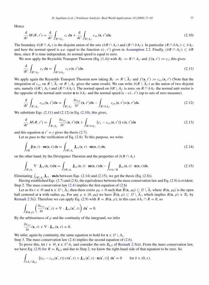
Fig. 4. One-dimensional sketch of the concentration. The meaning of ceq will be clarified in the sequel.
Finally, for the arbitrariness of δ, it follows that the integrand of the previous equation vanishes for every s ∈ ∂1 At .This give the second equation of system (2.6).Step 4. System (2.6) implies the mass conservation law (2.4).
This follows immediately from Eq. (2.9).
As already mentioned in the introduction, the second equation of system (2.6) has already appeared (see, e.g., VanDer Eerden [6]), following a different derivation. The basic system (2.6) is just an equivalent of the mass conservationlaw; we now add to this another physical law.
Assumption 2.8 (Fick’s First Law of Diffusion). The mass flow is proportional to the gradient of the concentration;more precisely,
Jex (x, t) = −D∇cex (x, t) for t ∈ Θ, x ∈ Ω \ At , (2.16)
where D > 0 is a constant coefficient (with base unit m2/s), called in the sequel the diffusion parameter.
Of course the previous assumptions could be generalized by replacing the constant D with a function D(x, t); howeversuch a generalization will not be considered in the sequel.
By substituting Eq. (2.16) in the first equation of System (2.6), we obtain the standard diffusion equation
∂cex
∂t(x, t) = D∆cex (x, t) for t ∈ Θ, x ∈ Ω \ At .
Moreover, the boundary condition on the moving boundary takes the form
(cs − cex (s, t)) v(s, t) = D∇cex (s, t) · n(s, t) for t ∈ Θ, s ∈ ∂1 At . (2.17)
In particular we can forecast the profile of the concentration in the surroundings of the boundary. By Assumption 2.4,(cs − cex (s, t)) > 0 for any s ∈ ∂At ; furthermore, if the crystal is growing, v(s, t) > 0. Therefore, by Eq. (2.17),∇cex (s, t) · n(s, t) > 0 during the growth. In Fig. 4 we sketch a typical one-dimensional profile for c.
2.3. Boundary and initial conditions
Supported by the empirical evidence we claim the following:
Assumption 2.9. The normal speed of the boundary ∂At is a function of the local concentration. In particular weassume that
v(s, t) = p(cex (s, t)− ceq)+ for t ∈ Θ, s ∈ ∂1 At , (2.18)
(see, e.g., Burger [14]), where
(cex − ceq)+
=
cex − ceq if cex > ceq0 otherwise.
(2.19)
D. Aquilano et al. / Nonlinear Analysis: Real World Applications 10 (2009) 71–92 79
Here: ceq ∈ (0, cs) is a constant, called the equilibrium concentration; p > 0 is another constant (with base unitmd+1/(mol s)), called kinetic parameter.
Remark 2.10. (i) From Eq. (2.18), we see that v(s, t) = 0 if cex (s, t) = ceq . That is, when the concentration reachesthe value ceq , crystals stop growing.
(ii) In the above we are assuming for the crystals an isotropic growth; in more general situations, p depends on thegrowth direction of the crystals.
(iii) Eq. (2.19) guarantees that crystals can only grow and Eq. (2.18) shows that the normal speed of the boundarylinearly depends on the deviation of the local concentration from the equilibrium value. Generally, we mightchoose other functional dependencies (see, e.g., Van Der Eerden [6]).
By substituting Eq. (2.18) in Eq. (2.17), we obtain a nonlinear Robin-type boundary condition on ∂At for cex , namely
∇cex (s, t) · n(s, t) = p(cex (s, t)− ceq)+ (cs − cex (s, t)) for t ∈ Θ, s ∈ ∂1 At .
To conclude let us discuss the initial concentration.
Assumption 2.11. At time t0 it is
cex (x, t0) = c0ex (x) > ceq ∀x ∈ Ω \ At0
(the above inequality meaning the mother phase is initially supersaturated). So, c(x, t0) = c0(x) for all x ∈ Ω , where
c0(x) :=
c0
ex (x) if x ∈ Ω \ At0 ,
cs if x ∈ At0 .
This concludes our list of assumptions for the deterministic part of the model. Let us observe that the assumptions donot account for the possibility that an existing crystal dissolves back in the mother phase.
2.4. Summing up
The results obtained so far can be summarized as follows.
Theorem 2.12. The Assumptions of this Section, about the crystals A = (At )t∈Θ and the concentration, imply thefollowing system for the pair (cex , A):
∂cex
∂t(x, t) = D∆cex (x, t) for t ∈ Θ, x ∈ Ω \ At ,
D∂cex
∂n(s, t) = p(cex (s, t)− ceq)
+(cs − cex (s, t)) for t ∈ Θ, s ∈ ∂At ,
cex (x, t0) = c0ex (x) for x ∈ Ω \ At0 .
(2.20)
The above system (2.20) contains the main equations of the model from the classical viewpoint. As anticipated, in thenext section we will rephrase these conclusions in a different framework, more suitable for numerical treatment.
3. Reformulation via distributions and level set equations
3.1. Preliminaries on distributions
Let us summarize the formalism of distributions on the torus (see, e.g., Dautray et al. [15] and Vladimirov [16]);our aim is mainly to fix some notations of subsequent use. Let us consider the test function space C∞(Ω), that wedenote by D(Ω) or, simply, D.
Definition 3.1. (i) A sequence fk ∈ D converges to f ∈ D when k → ∞ if the derivatives f (γ )k of any orderγ = (γ1, . . . , γn) converge uniformly on Ω to f (γ ).
80 D. Aquilano et al. / Nonlinear Analysis: Real World Applications 10 (2009) 71–92
(ii) We denote by D′(Ω) ≡ D′, the set of all linear functionals on D that are continuous with respect to theconvergence introduced on D. Any α ∈ D′ is called a generalized function or distribution and will be writtenas α : D → C, f 7→ 〈α, f 〉.
Regular distributions. Let us consider the space L1(Ω , dx) ≡ L1. Every function h ∈ L1 can be identified with thedistribution, denoted again with h, such that
〈h, f 〉 :=
∫Ω
h(x) f (x)dx ∀ f ∈ D. (3.1)
This defines a canonical embedding of the space L1 in D′ and we will say that the functional h ∈ D′ on the left-hand side of Eq. (3.1) is the canonical functional associated with the function h ∈ L1. When identified with thecorresponding functional in D′, a function h ∈ L1 will be called a regular distribution.Functional notations. Inspired by Eq. (3.1), it is common to denote the action of any distribution α as
〈α, f 〉 =
∫Ωα(x) f (x)dx. (3.2)
This is a mere notation since for a general α ∈ D′, there is no L1 function x 7→ α(x) fulfilling Eq. (3.2).Measures. Another class of distributions are measures. LetM(Ω) ≡M be the space of measures µ : B → C (recallthat B are the Borel subsets of Ω ). Any measure µ ∈ M induces a distribution, indicated with the same symbol,defined by
〈µ, f 〉 :=
∫Ω
f (x)µ(dx).
In the sequel we will be especially interested in Dirac measures. Let S ∈ B and let σ be the Hausdorff dimension ofS. We define the Dirac measure of S by
δS(·) := Hσ (S ∩ ·)
which is singular with respect to the d-dimensional Lebsesgue measure if σ < d. The corresponding distribution issuch that
〈δS, f 〉 =
∫S
f (x)Hσ (dx) ∀ f ∈ D. (3.3)
(This has been used, e.g., in Ambrosio et al. [17] and Capasso et al. [18]). As a special case, suppose S consists of asingle point x0; then σ = 0 and Eq. (3.3) becomes
〈δx0 , f 〉 = f (x0) ∀ f ∈ D.
Multiplication and distributions. As well known, an arbitrary distribution α ∈ D′ can be multiplied by a functiong ∈ D. The product gα ∈ D′ is defined by
〈gα, f 〉 := 〈α, g f 〉 ∀ f ∈ D.
Of course, distributions of some distinguish type can be multiplied by functions in more general classes than D. Forexample, a regular distribution h ∈ L1 can be multiplied pointwisely by a function g ∈ L∞(Ω), producing a regulardistribution hg ∈ L1(Ω). Another example of multiplication is given hereafter.Multiplication and measures. A measure µ ∈M can be multiplied by a bounded continuous function. More precisely,suppose k : dom(k) → C where dom(k) ∈ B and µ(supp (µ) \ dom (k)) = 0, with k|supp(µ)∩dom (k) bounded andcontinuous. Then kµ ∈M is such that
(kµ)(B) :=
∫B
k(x)µ(dx) ∀B ∈ B.
The corresponding distribution is such that
〈kµ, f 〉 =
∫Ω
k(x) f (x)µ(dx).
D. Aquilano et al. / Nonlinear Analysis: Real World Applications 10 (2009) 71–92 81
For example if µ = δS (so that supp(µ) = S), we have
〈kδS, f 〉 =
∫S
k(x) f (x)Hσ (dx).
Distributional derivatives. Let α ∈ D′, then the derivative ∂iα ∈ D′ is defined by
〈∂iα, f 〉 = −〈α, ∂i f 〉 ∀ f ∈ D.
By iteration, one can define the higher-order derivatives of α. For any multi-index γ = (γ1, . . . , γd), the derivative∂γ α := ∂
γ11 . . . ∂
γdd α is s.t.
〈∂γ α, f 〉 = (−1)|γ |〈α, ∂γ f 〉 ∀ f ∈ D. (3.4)
3.2. Indicator functions
Let IB ∈ L1 be the indicator function of B ∈ Reg s.t. IB(x) :=
1 if x ∈ B,0 otherwise. The corresponding distribution reads
〈IB, f 〉 =∫
B f (x)dx, ∀ f ∈ D. More generally, let h ∈ L1(B) and define h IB ∈ L1(Ω) by h IB(x) :=
h(x) if x ∈ B,0 otherwise.
The corresponding distribution is such that
〈 h IB, f 〉 =
∫B
h(x) f (x)dx ∀ f ∈ D.
Proposition 3.2. Let B ∈ Reg, h ∈ C1(B), then
∂i (h IB) = ∂i h IB − h mi δ∂B for i = 1, . . . , d, (3.5)
where m = (m1, . . . ,md) is the outward normal unit vector to ∂B. In particular if h = 1, then ∂i IB = −mi δ∂B .
Proof. Let f ∈ D. For i = 1, . . . , d , according to the general definition of distributional derivatives Eq. (3.4), wehave
〈∂i (h IB), f 〉 = −〈h IB, ∂i f 〉
= −
∫B
h(x)∂i f (x)dx. (3.6)
On the other hand, from the Leibnitz rule and the Gauss theorem
−
∫B
h(x)∂i f (x)dx =
∫B∂i h(x) f (x)dx −
∫B∂i (h(x) f (x)) dx
=
∫B∂i h(x) f (x)dx −
∫∂B
h(s)mi (s) f (s)ds
= 〈 ∂i h IB, f 〉 − 〈h mi δ∂B, f 〉. (3.7)
From Eqs. (3.6) and (3.7), we obtain the thesis.
In the sequel, we will often write Eq. (3.5) in the vector notation
∇(h IB) = ∇h IB − h m δ∂B . (3.8)
3.3. Time-dependent distributions
Definition 3.3. A time-dependent distribution is a family of distributions α ≡ (αt )t∈Θ with Θ an interval of R+. (αt )
belongs to the class Ck in a weak sense if, for any f ∈ D, the function t ∈ Θ 7→ 〈αt , f 〉 is Ck in the usual sense.Then the time derivative of α at t ∈ Θ is ∂αt
∂t ∈ D′ s.t.⟨∂αt
∂t, f
⟩:=
ddt
〈αt , f 〉 ∀ f ∈ D. (3.9)
82 D. Aquilano et al. / Nonlinear Analysis: Real World Applications 10 (2009) 71–92
Higher-order time derivatives are defined similarly.
Proposition 3.4. Let B = (Bt )t∈Θ be a regular time-dependent set moving with normal speed w. Let h ∈ C1(KB,C)and consider the family (h(·, t)IBt )t∈Θ where IBt is the indicator function of Bt . This is a C1 time-dependentdistribution, and
∂
∂t(h(·, t)IBt ) =
(∂h
∂t(·, t)
)IBt + (hw)(·, t)δBt . (3.10)
In particular, if h = 1, thendIBt
dt = w(·, t)δ∂Bt .
Proof. Consider any f ∈ D; then
ddt
〈h(·, t)IBt , f 〉 =ddt
∫Bt
h(x, t) f (x)dx.
We now apply the Reynolds Transport Theorem, giving
ddt
∫Bt
h(x, t) f (x)dx =
∫Bt
∂h
∂t(x, t) f (x)dx +
∫∂Bt
h(s, t)w(s, t) f (s)ds
=
⟨ (∂h
∂t(·, t)
)IBt , f
⟩+ 〈(hw)(·, t)δBt , f 〉.
3.4. Preparing applications to our model
Let us return to the framework of the previous section invoking a moving crystal phase (At ). As in Assumption 2.2we refer to n(·, t) and v(·, t) as the outward normal unit and the normal speed, respectively. We can rephrase Eqs.(2.2) and (2.5) for the concentration and the mass flow as
c(·, t) = cs IAt + cex (·, t)IΩ\At for t ∈ Θ (3.11)
and J i (·, t) = J iex (·, t)IΩ\At , i.e., in vector form,
J(·, t) = Jex (·, t)IΩ\At for t ∈ Θ . (3.12)
Eqs. (3.11) and (3.12) hold everywhere in Ω . From now on, for a clearer outline, we omit the indication of the timedependence: for example, Eq. (3.11) will be written as c = cs IAt + cex IΩ\At .
Lemma 3.5. Due to Assumptions 2.2, 2.4 and 2.6, c and J are time-dependent distributions of classes C2 and C1
respectively. Their distributional derivatives are given by
∂c
∂t=∂cex
∂tIΩ\At + v(cs − cex )δ∂At , (3.13)
∇ · J = (∇ · Jex )IΩ\At + Jex · n δ∂At . (3.14)
Proof. All statements are direct consequences of Eq. (3.11) and Proposition 3.4 and of Eq. (3.12) and Proposition 3.2,respectively.
3.5. Distributional formulation of system (2.6)
Proposition 3.6. System (2.6) is equivalent to the equation
∂c
∂t= −∇ · J (3.15)
(again, to be interpreted as an equality of time-dependent distribution on Ω ).
D. Aquilano et al. / Nonlinear Analysis: Real World Applications 10 (2009) 71–92 83
Proof. By taking the sum side by side of Eqs. (3.13) and (3.14), we obtain
∂c
∂t+ ∇ · J =
(∂cex
∂t+ ∇ · Jex
)IΩ\At + ((cs − cex )v + Jex · n) δ∂At . (3.16)
By comparison with system (2.6), we get the thesis.
3.6. Rephrasing the Fick law via extended multiplication of distributions
Let us combine Eq. (3.12) with the Fick law (2.16); in this way we obtain the equation
J = −D (∇cex ) IΩ\At (3.17)
holding everywhere on Ω and referred to as the extended Fick law. On the other hand, Proposition 3.2 implies
∂i c = (∂i cex ) IΩ\At − (cs − cex )ni δ∂At (3.18)
whence
(∇cex ) IΩ\At = ∇c + csnδ∂At − cex nδ∂At . (3.19)
We now want to rewrite the last term on the right-hand side in terms of c only, so that Eq. (3.15) reads as a diffusionequation with respect to the only unknown c.
In order to obtain a further relation between cδ∂At and cexδ∂At , we need to extend the classical Schwartz theory. Inparticular we define the product between a Dirac δ-distribution and a discontinuous function as it follows.
Definition 3.7. Let S ∈ B with Hausdorff dimension d − 1; suppose there exists a connected open subset R ⊂ Ωs.t. S = ∂R. Let µ ∈ M with support on S and let g : Ω → R be a function continuous outside S, with a jumpdiscontinuity of the first type through S (i.e. g ∈ C(Ω \ R) and g ∈ C(R)). The product gµ ∈M is defined by
gµ := gavµ, (3.20)
where gav ∈ C(S,R) is given by
gav(s) :=12
(limx→sx∈R
g(x)+ limx→s
x∈Ω\R
g(x)
)for s ∈ S. (3.21)
Similar prescriptions can be found frequently in the physical literature, see, e.g., Goodman [19] (dealing with the caseΩ = R and S = x0, x0 ∈ R). By continuity, the average value of the jump in c for any point s ∈ ∂At is exactly12 (cs + cex )(s). Hence, by Eq. (3.21), the product between the Dirac δ-functional δ∂At and the discontinuous functionc reads
c δ∂At =12(cs + cex )δ∂At . (3.22)
We now substitute Eq. (3.22) in Eq. (3.19) and we obtain
(∇cex ) IΩ\At = ∇c + cs n δ∂At − 2cnδ∂At + csnδ∂At .
Finally, by Eq. (3.13), the previous equation reads
(∇cex ) IΩ\At = ∇c − 2(cs − c)∇ IAt . (3.23)
Summing up, we have
Proposition 3.8. The extended Fick law is equivalent to
J = −D∇c + 2D(cs − c)∇ IAt . (3.24)
84 D. Aquilano et al. / Nonlinear Analysis: Real World Applications 10 (2009) 71–92
By substituting Eq. (3.24) in Eq. (3.15), we formally obtain a diffusion equation in Ω in terms of c and of the indicatorfunction IAt . More precisely:
Corollary 3.9. Eq. (2.6) and the extended Fick law (3.17) imply
∂c
∂t= D∆c − 2D ∇ ·
((cs − c)∇ IAt
). (3.25)
The second term on the right-hand side acts as a sink term in the diffusion equation. In fact it represents the effects ofthe moving boundary and accounts the amount of matter absorbed by the growing crystal.
3.7. Level set equation
Definition 3.10. Let (Bt )t∈Θ be a time-dependent regular set. A level set function is a function φ : Ω × Θ → R s.t.
φ(x, t)
< 0 if x ∈ Bt ,
> 0 if x 6∈ Bt ,= 0 if x ∈ ∂Bt ,
and φ possesses the following regularity: if t ∈ Θ and s ∈ ∂1 Bt , then φ is C1 with nonzero
gradient on an open neighborhood of (s, t).
Proposition 3.11. If (Bt )t∈Θ , φ are as in the previous definitions and m(·, t), w(·, t) are the normal unit vector andthe normal speed of Bt , respectively, then
∂φ
∂t(s, t)+ |∇φ(s, t)|w(s, t) = 0 for t ∈ Θ, s ∈ ∂1 Bt . (3.26)
Proof. By recalling Definition 1.2, we have
∂Bt ′ = Φt ′,t (∂Bt ), (3.27)
where t is fixed and t ′ ∈ I (t, ς). By definition
φ(s′, t ′) = 0 ∀s′∈ ∂Bt ′ .
In particular, let s ∈ ∂1 Bt ; then, since s′= Φt ′,t (s) ∈ ∂Bt , we have
φ(Φt ′,t (s, t ′)) = 0. (3.28)
We now take the time derivative of Eq. (3.28) with respect to t ′ for t ′ = t (by recalling that Φt,t (s) = s), and we applythe chain rule
∂φ
∂t(s, t)+ ∇φ(s, t) ·
∂Φt ′,t
∂t ′
∣∣∣∣t ′=t
(s) = 0.
The gradient vector ∇φ has the same direction of the normal unit vector to the boundary, i.e.,
m(s, t) =∇φ(s, t)
|∇φ(s, t)|; (3.29)
hence
∂φ
∂t(s, t)+ |∇φ(s, t)| m(s, t) ·
∂Φt ′,t
∂t ′
∣∣∣∣t ′=t
(s) = 0. (3.30)
From Eq. (3.30) and the definition of the normal speed, we obtain the thesis.
Let us return to our model, and suppose φ is a level set function for the crystals A = (At )t∈Θ . Then, we can writeEq. (3.26) with the usual notation v for the normal speed, i.e.,
∂φ
∂t(s, t)+ |∇φ(s, t)|v(s, t) = 0 for t ∈ Θ, s ∈ ∂1 At . (3.31)
D. Aquilano et al. / Nonlinear Analysis: Real World Applications 10 (2009) 71–92 85
By substituting Eq. (2.18) in Eq. (3.31), we obtain
∂φ
∂t(s, t)+ |∇φ(s, t)|p(c(s, t)− ceq)
+= 0 for t ∈ Θ, s ∈ ∂1 At . (3.32)
For subsequent use, let us observe that the indicator function of At can be viewed as a functional of the level setfunction φ, namely
IAt = I [φ], I [φ](x, t) :=
1 if φ(x, t) < 0,0 if φ(x, t) ≥ 0.
(3.33)
3.8. Main theorem
By collecting the results of this section, the following theorem is proved.
Theorem 3.12. Let us consider all the assumptions of Section 2, about the crystals A = (At )t∈Θ and theconcentration. Furthermore, suppose there is a level set function φ for A; then, the pair (c, φ) fulfils the followingsystem
∂c
∂t(x, t) = D∆c(x, t)− 2D ∇ · ((cs − c(x, t))∇ I [φ](x, t)) for (x, t) ∈ Ω × Θ,
∂φ
∂t(s, t)+ |∇φ(s, t)|p(c(s, t)− ceq)
+= 0 for s ∈ φ(·, t)−1(0), t ∈ Θ,
c(x, t0) = c0(x) for x ∈ Ω ,
(3.34)
where the functional I [φ] reads as in Eq. (3.33); the first equation in (3.34) must be intended as an equality oftime-dependent distributions (and is written in the functional notations only for simplicity).
The above system, based on distributions and level sets, plays a role similar to system (2.20), relying on a moreclassical language.
Practically, in the spirit of general level set methods (see, e.g., Osher et al. [20] and Sethian [21]), in numericalsimulations we will search for a function φ fulfilling the second equation everywhere on Ω × Θ (except possibly thenonregular point of ∂At ).
3.9. Nondimensional equations
We now rescale the variables introduced so far with respect to some typical values. Let ξ be the mean free path ofa particle in the solution; that is, ξ is the average distance that any particle travels between any collision with otherparticles. Let D be the diffusion coefficient and ceq be the equilibrium concentration, then we define the followingvariables
x =xξ
t =2D
ξ2 t c(x, t) =1
ceqc
(xξ,
2D
ξ2 t
).
In particular
∂ c
∂ t(x, t) =
1ceq
ξ2
2D
∂c
∂t
(xξ,
2D
ξ2 t
)and
∆c(x, t) =ξ2
ceq∆c
(xξ,
2D
ξ2 t
).
Therefore, the nondimensional diffusion equation reads
∂ c
∂ t(x, t) =
12∆c(x, c)− ∇ ·
((cs − c(x, t))∇ IAt
(x)).
86 D. Aquilano et al. / Nonlinear Analysis: Real World Applications 10 (2009) 71–92
Let v be the normal speed defined obviously in terms of the nondimensional variables (x, t), then Eq. (2.18) can berephrased as
v = p(c(x, t)− 1)+, p := (ξ/2D)ceq p.
4. The nucleation process
We now complete the growth–diffusion equations by modeling the nucleation of the new crystals with a stochasticbirth process. At the molecular scale, crystallization is the effect of the movement, aggregation and disaggregationof basic components, called Growth Units. In the mother phase Growth Units diffuse until they join together andconstitute aggregates. Once their size overcomes a critical threshold, they eventually become stable originating a newgerm, namely a critical nucleus, otherwise they dissolve back in the mother phase, see, e.g., Abbona et al. [22], Gilmeret al. [23] or Micheletti et al. [24].
In our model we only consider the stable nuclei; that is, we can only observe the aggregates that, once formed,grow into crystals and do not dissolve back in the mother phase. Since the shape of a critical nucleus depends on itsinner chemical structure only and the crystal phase is mono-component, all the critical nuclei have the same shape.The size of each critical nucleus generally depends on local properties, e.g., the supersaturation, and in general it isgreater than zero at the instant of birth. Hence it is not realistic to represent the new germs with points and the outcomeof a nucleation process reads as the following triple
(X j , τ j , A jτ j) ( j ∈ J )
for some index set J ⊆ N, where A jτ j represents the set occupied by the critical nucleus born at the (random) time τ j
and X j ∈ Ω is the (random) spatial location of its center (e.g., the center of mass).Real experiments show that new germs occur randomly in space and time in the mother phase. We define a
stochastic space–time point process whose outcomes give the location of the center of the critical nuclei and theirtime of occurrence. Then we analyze the geometry of the critical nuclei and we define a realization of the nucleationprocess by centering the nucleus in the corresponding space–time coordinates.
4.1. Marked point processes
Let Θ = [0, t f ) be the time interval of observation, let B(Θ) ≡ BΘ be its associated Borel σ -algebra and let
B(Ω) ≡ BΩ be the Borel σ -algebra associated with Ω . We define a Marked Point Process on Θ = [0, t f ) with markspace (Ω ,BΩ ) (see, e.g., Capasso et al. [25] and Daley et al. [26]) as
N =
∑j∈J
δX j ,τ j .
Here:
• τ j is a positive random variable on (Θ,BΘ ) representing the time of occurrence of the j th critical nucleus;• X j is a random variable on (Ω ,BΩ ) representing the spatial location of the center of the critical nucleus born at
time τ j ;• J ⊆ N is an index set;• δx,t is the Dirac measure on BΩ ⊗ BΘ centered at (x, t).
It will be useful to define the stochastic process
Nt (B) := N (B × [0, t]) (B ∈ BΩ )
and the filtration (suitably completed)
Ft := σ Ns(B): 0 ≤ s ≤ t, B ∈ BΩ (t ∈ Θ);
the latter is such that
Ft ⊂ F for t ≥ 0; Fs ⊂ Ft for 0 ≤ s < t.
D. Aquilano et al. / Nonlinear Analysis: Real World Applications 10 (2009) 71–92 87
We also define, for all t ∈ Θ , the σ -algebras
Ft− = σ Ns(B): 0 ≤ s < t, B ∈ BΩ ;
then
P(∆N = 1 | Ft−) = λ(x, t)dx dt,
where λ(x, t) is the space–time-dependent intensity of the point process.
4.2. The geometry of the critical nuclei
Since all the critical nuclei have the same shape, we refer to the equivalence class of the sets representing the nucleias the typical nucleus or the primary grain (see Serra [27]). In particular the shape of the primary grain is the so-calledWulff shape (see, e.g., Peng et al. [28]).
Assumption 4.1 (Gibbs Rule). Let the shape of the typical nucleus be a sphere or a regular polygon and let r be theradius of the circumscribed sphere to the critical nucleus. If a birth occurs in x ∈ Ω at time t ∈ Θ ; then
r(x, t) =2σV
∆µ(x, t), (4.1)
where σ is the surface free energy, V is the molar volume (such that V = 1/cs) and ∆µ > 0 is the supersaturation onthe new formed boundary.
The birth of new crystals can only occur where the local concentration c(x, t) is greater than the equilibrium value ceqand the supersaturation is given by
∆µ(x, t) = kT ln(
c(x, t)
ceq
),
where k is the Boltzmann constant and T is the temperature that we approximate with a constant value throughout theprocess. Hence the critical radius is defined only for c(x, t) > ceq and given by
r(x, t) =2σ
kT cs ln(
c(x,t)ceq
) for t ∈ Θ, x ∈ Ω . (4.2)
The Gibbs rule can be also generalized to the case of nonregular polygons, such as parallelotopes.Since two crystals cannot be born in the same position almost surely, once the typical shape is given, each critical
nucleus is completely determined by its center, orientation and size. The nucleation process can also be defined as aninfinitesimal Boolean process (see Jeulin [29]).
4.3. The intensity of the process
We assume that the Marked Point Process N is a Poisson process whose intensity λ(x, t) depends on the stochasticgeometry of the overall process (see, e.g., Capasso et al. [25] and references therein), hence we will refer to N as adoubly stochastic Poisson point process. Moreover, we assume that the following equations hold (see Bremaud [30]and Last et al. [31]) for any [t1, t2] ⊂ Θ :
0 ≤
∫ t2
t1
∫Ωλ(x, t)dx dt < +∞, (4.3)∫
+∞
0
∫Ωλ(x, t)dx dt = +∞. (4.4)
Eq. (4.3) ensures that the process is a.s. locally finite, while Eq. (4.4) guarantees that at least one event occurs inΩ × R+.
Experimental evidence suggests the following assumptions:
88 D. Aquilano et al. / Nonlinear Analysis: Real World Applications 10 (2009) 71–92
Assumption 4.2. (i) births may occur in the mother phase only;(ii) it is almost surely impossible that a new germ occurs within a given distance b > 0, called inhibition distance,
from an already formed crystal;(iii) there is a higher probability of nucleation where the density of matter is higher.
From a physical point of view, below a given threshold for the concentration, namely cthr > ceq , the aggregates a.s.dissolve back in the mother phase, without originating a stable nucleus, while above this threshold there is a positiveprobability of formation of a stable nucleus. Let r(x, t) be the radius of a critical nucleus born at (x, t). Then theintensity of the process N is given by
λ(x, t) =
f (c(x, t)) if x ∈ Ω \ At and d(x, ∂At ) > r(x, t)+ b,0 otherwise,
(4.5)
for t ∈ Θ , where d(x, ∂At ) is the Hausdorff distance between x and ∂At and f : R+→ R+ is a suitable function. In
the three-dimensional case, empirical evidence suggests an exponential behaviour for the function f as follows
f (c) = D
(kT
σ
) 32 c8/3
s
4π
(ln(
c
ceq
))2
exp
−16πσ 3
3 (kT )3(
cs ln( cceq))2
for c > ceq , where we have used the same notations of Eq. (4.2).
5. Birth and growth model
We finally merge in a unique birth and growth model the equations derived so far. The diffusion, growth andnucleation processes cannot in general be decoupled since the indicator function of At in the diffusion and growthequations changes at each random nucleation. Moreover the intensity function of the nucleation process depends onthe concentration and it has support in the mother phase only.
5.1. Piecewise deterministic process
Every time a birth occurs, new initial conditions for the concentration c and for the set At are given. Then thesystem evolves up to the next nucleation following the growth and diffusion Eq. (3.34).New nuclei. The time of occurrence of each critical nucleus is given by the random variable τ j that, since N isa Poisson process, has an exponential distribution. When a birth occurs the set At , representing the crystal phase,changes and can be defined as
At =
⋃τ j ≤t
A jt , (5.1)
where the set A jt represents the crystal born at time τ j and grown up to time t . We define A j
t = ∅ for any t < τ j ; of
course A jτ j is just the crystal at the time of birth. Let τ0 > 0 be the first time of nucleation such that At = ∅ for any
t ∈ [0, τ0); hence the growth Eq. (3.32) is not defined for t ∈ [0, τ0). On the other hand, the diffusion Eq. (3.25) holdsfor any t ∈ Θ .Corrections for the concentration. When a birth occurs, the constituent mass of the critical nucleus is soaked fromthe mother phase. In particular the value of the concentration in the crystal phase is higher than the value of theconcentration anywhere in the mother phase. Hence, since the physical system is closed and the mass must bepreserved, the average concentration in the mother phase must decrease, especially in the region surrounding thesite of the new nuclei. We take into account this compensation effect in our model by correcting the value of theconcentration at each nucleation, in particular we choose to decrease the value of the concentration in a small regionsurrounding the new nucleus as it follows.
Let A jτ j be the set representing the critical nucleus born at time τ j , and let τ−
j be a time preceding τ j of aninfinitesimal quantity. Since the mass must be preserved, the following equation holds∫
Ωc(x, τ−
j )dx =
∫Ω
c(x, τ j )dx.
D. Aquilano et al. / Nonlinear Analysis: Real World Applications 10 (2009) 71–92 89
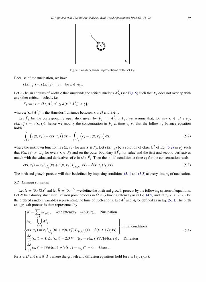
Fig. 5. Two-dimensional representation of the set F j .
Because of the nucleation, we have
c(x, τ−
j ) < c(x, τ j ) = cs for x ∈ A jτ j.
Let F j be an annulus of width ζ that surrounds the critical nucleus A jτ j (see Fig. 5) such that F j does not overlap with
any other critical nucleus, i.e.,
F j := x ∈ Ω \ A jτ j
: 0 ≤ d(x, ∂A jτ j) < ζ ,
where d(x, ∂A jτ j ) is the Hausdorff distance between x ∈ Ω and ∂A j
τ j .
Let F j be the corresponding open disk given by F j = A jτ j ∪ F j ; we assume that, for any x ∈ Ω \ F j ,
c(x, τ−
j ) = c(x, τ j ); hence we modify the concentration in F j at time τ j so that the following balance equationholds ∫
F j
(c(x, τ−
j )− c(x, τ j ))
dx =
∫A jτ j
(cs − c(x, τ−
j ))
dx, (5.2)
where the unknown function is c(x, τ j ) for any x ∈ F j . Let c(x, τ j ) be a solution of class C2 of Eq. (5.2) in F j suchthat c(x, τ j ) > ceq for every x ∈ F j and on the outer boundary ∂ F j , its value and the first and second derivativesmatch with the value and derivatives of c in Ω \ F j . Then the initial condition at time τ j for the concentration reads
c(x, τ j ) = cs IA jτ j(x)+ c(x, τ−
j )IΩ\A jτ j(x)− c(x, τ j )IF j (x). (5.3)
The birth and growth process will then be defined by imposing conditions (5.1) and (5.3) at every time τ j of nucleation.
5.2. Leading equations
Let Ω = (R/ lZ)d and let Θ = [0, t f ), we define the birth and growth process by the following system of equations.Let N be a doubly stochastic Poisson point process in Ω × Θ having intensity as in Eq. (4.5) and let τ0 < τ1 < · · · bethe ordered random variables representing the time of nucleations. Let A j
t and At be defined as in Eq. (5.1). The birthand growth process is then represented by
N =
∑j∈J
δX j ,τ j , with intensity λ(c(x, t)), Nucleation
Aτ j =
⋃k≤ j
Akτ j,
c(x, τ j ) = cs IA jτ j(x)+ c(x, τ−
j )IΩ\A jτ j(x)− c(x, τ j ) IF j (x),
Initial conditions
∂c
∂t(x, t) = D∆c(x, t)− 2D ∇ · ((cs − c(x, t))∇ I [φ](x, t)) , Diffusion
∂φ
∂t(s, t)+ |∇φ(s, t)|p (c(s, t)− ceq)
+= 0, Growth
(5.4)
for x ∈ Ω and s ∈ ∂1 At , where the growth and diffusion equations hold for t ∈ [τ j , τ j+1).
90 D. Aquilano et al. / Nonlinear Analysis: Real World Applications 10 (2009) 71–92
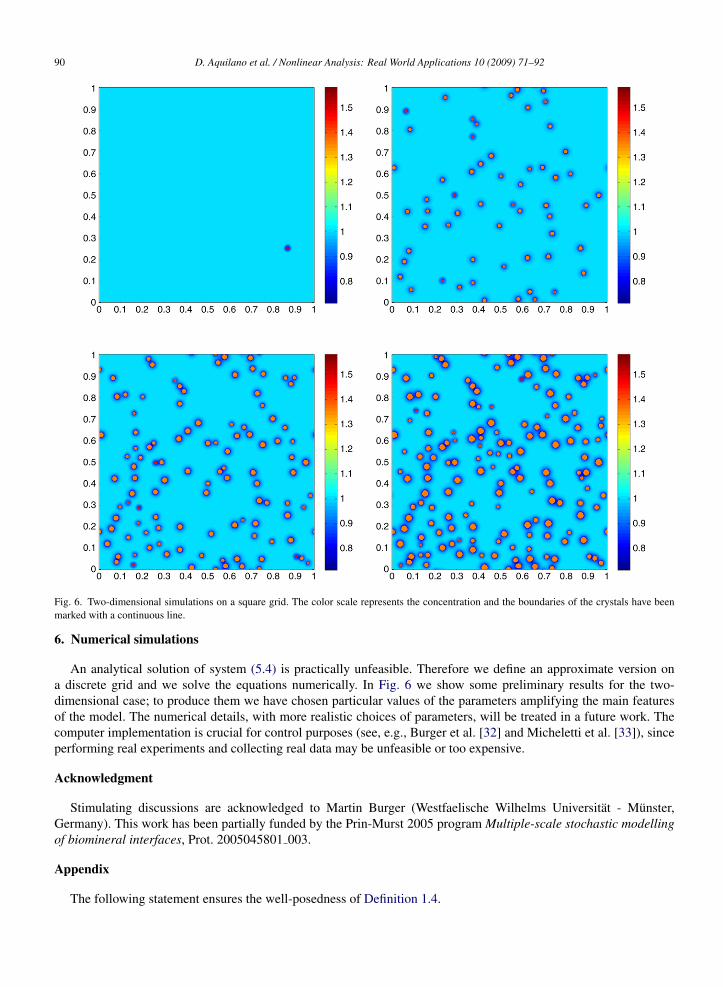
Fig. 6. Two-dimensional simulations on a square grid. The color scale represents the concentration and the boundaries of the crystals have beenmarked with a continuous line.
6. Numerical simulations
An analytical solution of system (5.4) is practically unfeasible. Therefore we define an approximate version ona discrete grid and we solve the equations numerically. In Fig. 6 we show some preliminary results for the two-dimensional case; to produce them we have chosen particular values of the parameters amplifying the main featuresof the model. The numerical details, with more realistic choices of parameters, will be treated in a future work. Thecomputer implementation is crucial for control purposes (see, e.g., Burger et al. [32] and Micheletti et al. [33]), sinceperforming real experiments and collecting real data may be unfeasible or too expensive.
Acknowledgment
Stimulating discussions are acknowledged to Martin Burger (Westfaelische Wilhelms Universitat - Munster,Germany). This work has been partially funded by the Prin-Murst 2005 program Multiple-scale stochastic modellingof biomineral interfaces, Prot. 2005045801 003.
Appendix
The following statement ensures the well-posedness of Definition 1.4.
D. Aquilano et al. / Nonlinear Analysis: Real World Applications 10 (2009) 71–92 91
Proposition A.1. Let t ∈ Θ , s ∈ ∂1 Bt . Then, w(s, t) := w(s, t) · m(s, t) does not depend on the choice of the familyof diffeomorphisms in Eq. (1.1).
Proof (Sketch). Consider two families of diffeomorphisms φt ′,t , ψt ′,t as in Definition 1.2. Defining w(s, t) :=∂φt ′,t∂t |t ′=t
, q(s, t) :=∂ψt ′,t∂t |t ′=t
, we want to prove that
w(s, t) · m(s, t) = q(s, t) · m(s, t). (A.1)
We can locally represent the boundary in terms of a C1 function f with nonvanishing gradient, so that ∂Bt ′ = s′|
f (s′, t ′) = 0; for example take f (s′, t ′) := yd(s′)− F(y1(s′), . . . , yd−1(s′), t ′) with F as in Remark 1.3. Hence,
f (φt ′,t (s, t ′)) = 0, f (ψt ′,t (s, t ′)) = 0. (A.2)
We now take the derivatives of Eq. (A.2) with respect to t ′ at t ′ = t ; this gives
∇ f (s, t) · w(s, t)+∂ f
∂t ′(s, t) = 0, ∇ f (s, t) · q(s, t)+
∂ f
∂t ′(s, t) = 0.
But m(s, t) =∇ f|∇ f |
(s, t); this fact, with the previous equation, implies
(|∇ f |m · w) (s, t) = (|∇ f |m · q) (s, t),
whence the thesis (A.1).
References
[1] D. Ramkrishna, Population Balances, Academic Press, San Diego, 2000.[2] A.E. Nielsen, Kinetics of Precipitation, Pergamon Press, Oxford, 1964.[3] C. Wert, C. Zener, Interference of growing spherical precipitate particles, J. Appl. Phys. 21 (1950) 5–8.[4] C. Noguera, B. Fritz, A. Clement, A. Baronnet, Nucleation, growth and ageing scenarios in closed systems I: A unified mathematical
framework for precipitation, condensation and crystallization, J. Cryst. Growth 297 (2006) 180–186.[5] C. Noguera, B. Fritz, A. Clement, A. Baronnet, Nucleation, growth and ageing scenarios in closed systems II: Dynamics of a new phase
formation, J. Cryst. Growth 297 (2006) 187–198.[6] J.P. Van Der Eerden, Crystal growth mechanisms, in: D.T.J. Hurle (Ed.), Handbook of Crystal Growth, vol. 1a, North Holland, Amsterdam,
1993, pp. 307–475.[7] M. Giaquinta, G. Modica, Analisi matematica 4. Funzioni di piu variabili, Pitagora, Bologna, 2005. English version in press by Birkhauser.[8] A. Miranville, R. Temam, Modelisation mathematique et mecanique des milieux continus, Springer, Berlin, 2003.[9] M. Burger, V. Capasso, C. Salani, Modelling multi-dimensional crystallization of polymers in interaction with heat transfer, Nonlinear Anal.
Real World Appl. 3 (2002) 139–160.[10] M. Burger, V. Capasso, L. Pizzocchero, Mesoscale averaging of nucleation and growth model, SIAM J. Multiscale Model. Simul. 5 (2006)
564–592.[11] V. Capasso (Ed.), Mathematical modelling for polymer processing, in: Polymerization, Crystallization, Manufacturing, Series: Mathematics
in Industry, vol. 2, Springer, Heidelberg, 2002.[12] P. Colli, C. Verdi, A. Visintin (Eds.), Free Boundary Problems, in: Theory and Applications, Birkhauser Verlag, Basel, 2000.[13] M. Rubbo, Spiral growth limited by surface kinetics. A self-consistent model, J. Cryst. Growth 223 (2001) 235–250.[14] M. Burger, Growth of multiple crystals in polymer melts, European J. Appl. Math. 15 (2004) 347–363.[15] R. Dautray, J.-L. Lions, Analyse mathemathique et calcul numerique pour les sciences et les techniques, tome 1, Masson, Paris, 1984.[16] V.S. Vladimirov, Equations of Mathematical Physics, Marcel Dekker, New York, 1971.[17] L. Ambrosio, V. Capasso, E. Villa, On the approximation of geometric densities of random closed sets, Preprint, RICAM Report, Linz (2006).[18] V. Capasso, E. Villa, On the continuity and absolute continuity of random closed sets, Stoch. Anal. Appl. 24 (2006) 381–397.[19] J.W. Goodman, Introduction to Fourier optics, McGraw, San Francisco, 1968.[20] S. Osher, R. Fedkiw, Level set Methods and Dynamic Implicit Surfaces, Springer, New York, 2003.[21] J.A. Sethian, Level set methods, in: Evolving Interfaces in Geometry, Fluid Mechanics, Computer Vision and Materials Science, Cambridge
University Press, 1996.[22] F. Abbona, D. Aquilano, Morphology of crystals grown from solution, in: M. Dudley (Ed.), Springer Handbook of Crystal Growth, Defects
and Characterization, Springer-Verlag, Heidelberg, 2007.[23] G.H. Gilmer, P. Bennema, Computer simulation of crystal surface structure and growth kinetics, J. Cryst. Growth 13–14 (1972) 148–153.[24] A. Micheletti, S. Patti, E. Villa, Crystal growth simulations: A new mathematical model based on the Minkowski sum of sets, in: D. Aquilano,
et al. (Eds.), Industry days 2003-2004, Series: The Miriam Project, Esculapio, Bologna, 2005, pp. 130–140.[25] V. Capasso, A. Micheletti, et al., Stochastic geometry of spatially structured birth and growth processes. Application to crystallization
processes, in: V. Capasso (Ed.), Topics in Spatial Stochastic Processes, in: Series: Lecture notes in Mathematics, Springer, Berlin, 2003,pp. 1–39.

92 D. Aquilano et al. / Nonlinear Analysis: Real World Applications 10 (2009) 71–92
[26] D.J. Daley, D. Vere-Jones, An Introduction to the Theory of Point Processes, Springer-Verlag, New York, 1988.[27] J. Serra, N.A.C. Cressie, Image Analysis and Mathematical Morphology, London Academic Press, 1984.[28] D. Peng, S. Osher, B. Merriman, H. Zhao, The geometry of Wulff Crystals Shapes and its relations with Riemann problems, Preprint, UCLA
CAM Report (1998).[29] D. Jeulin, Modelling random media, Image Anal. Stereol. 21 (2002) 31–40.[30] P. Bremaud, Point processes and queues, in: Martingale Dynamics, Springer-Verlag, New York, 1981.[31] G. Last, A. Brandt, Marked Point Processes on the Real Line: The Dynamic Approach, Springer-Verlag, New York, 1995.[32] M. Burger, V. Capasso, A. Micheletti, Optimal control of polymer morphologies, J. Engrg. Math. 49 (2004) 339–358.[33] A. Micheletti, M. Burger, Stochastic and deterministic simulation of nonisothermal crystallization of polymers, J. Math. Chem. 30 (2001)
169–193.