A Bi-phase Approach for the Combined Production

and Distribution Problem

Nejah Ben Mabrouk Bassem J arboui

FSEGS, route de l' aroport km4,

Sfax 3018, Tunisia

Email: mabrouknejah@gmail.com

Email: bassemjarboui@yahoo.fr

Abstract-In this paper, we are interested to the problem of the production distribution planning in supply chain man­agement while minimizing three costs simultaneously such as production setups, inventories and distribution. The complexity of this problem is known to be NP-hard. In order to solve this problem, we propose a bi-phase Variable Neighbourhood Search algorithm (VNS). The computational experiments, according to the instances of the literature, have shown the effectiveness of our proposed algorithm against the existing approaches.

I. INTRODUCTION

The integrated production distribution problem (IPDP) is to determine the operation planning to coordinate the production, inventory and transportation routing operations so that the customer demand, transporter capacity, plant production and inventory and customer inventories constraints are all satisfied, while the resulting cost (sum of production, inventory and transportation cost) over a given planning horizon is min­imised.

The problem is defined on a complete weighted and undi­rected network G = (N,E,C), in which N(VO,Vl, ... ,Vn) is a set of nodes indexed from 0 onwards. Node 0 is a

plant with limited fleet of identical vehicles of capacity W. E = {(Vi,Vj): Vi,Vj E N,i #j} is a set of edges and the

weight Cij = Cji on each edge (i,j) denotes the travelling cost between nodes i and j.

The plant manufactures one single product to supply the customers over a planning horizon T subdivided into T + 1 periods or days, indexed from 0 to T. The initial dummy period indexed by 0 is used for initial inventories. The daily production is limited to a value P PC (plan production capac­

ity). If production is decided in a given day t, one fixed setup cost s is incurred. The product may be either stored at the plan inventory, with a storage cost h per unit of product and per period, or shipped to customers. We not that, the setup and

inventory costs are not time dependent.The product may be stored at the plan with a limited storage capacity PSC (Plan Storage Capacity). It may be also distributed to customers using the fleet of homogeneous vehicles. The vehicle capacity is limited to a value W. The demand for each customer i is known for each day t. Each customer has a limited storage capacity (Customer Storage Capacity). Inventory holding costs

Mansour Eddaly Habib Chabchoub

FSEGS, route de l'aroport km4,

Sfax 3018, Tunisia

Email: eddaly.mansour@gmail.com

Email: habib.chabchoub@fsegs.mu.tn

at customers are supported by them and not considered in the problem. Shortages are not allowed. Each customer can be serviced at most once per day and each vehicle of fleet is limited to one trip per day, hence there can be up to trips per day.

To impose in each period the order between production and distribution activities, deliveries take place in the morning, before a production run at the plant and before the customers' daily consumption. The production of each day is available the next morning. This convention is common in production

planning models to simplify inventory balance equations and to know when storages costs must be counted.

The objective is to detemline, for each period, the amount produced, the quantities shipped to each customer and the delivery trips to minimise the total cost (production setups,

inventory holding costs and transportation costs). The IPDP is NP-hard, since it reduces to the periodic vehicle routing problem (PVRP) which is a particular case obtained if setup and storage costs are ignored. Note that the PVRP is known to be NP-hard (Christofides and Beasley, 1984).

Two approaches have been proposed in the literature to solve the IPDP. The first one is a bi-phase algorithm proposed

by Boudia et al. (2008). The second one is an integrated approach proposed by Boudia et al. (2007) and Boudia and Prins (2009). In this paper, our interest is focused on the first approach (biphase), we propose an effective algorithm which gave superior results compared with the two phase and integrated approaches proposed in the literature.

In our algorithm, the first phase leads to optimizing the plan

of production whereas the second phase is devoted to optimize

the routing problem. These two phases are not independent, therefore while minimizing the production and the inventory costs, our algorithm attempts to minimize the number of deliveries for each client. In such way, the phase of routing is taken into account in the phase of production planning.

II. LITERATURE REVIEW

The early model dealing with coordination problems be­tween production and distribution activities was developed by Dror and Ball for a propane distribution company. Dror and Ball take in their work the example of one plant producing

978-1-61284-4577-0324-9/11/$26.00 ©2011 IEEE 216

propane and delivering it to different customers over a muti­period horizon. The solution approach involves successive solution of a single period model, with a cost adjustment over successive periods. This method is similar to the rolling horizon technique well known in production planning. Other works like Jayaraman and Pirkul take into consideration the case of truckload deliveries to avoid the problems raised by the vehicle routing problem.

Chandra and Fisher (1994) developed an optimization ap­proach for IPDP. It considered the problem with several prod­ucts, unlimited plant storage capacity and fleet size, deliveries can be made on different occasions to the same customers using different vehicles and the absence of holding cost at the plant. Plan storage capacity is limited and the presence of inventory holding cost. An integrated approach is proposed and compared to a two phase approach. Saving between 3% and 20% are reported on instances with up to 10 products, 50 customers and 10 periods.

In another work Chandra (1993), treats the problem of preparation of orders in a regional warehouse to guarantee the demands of customers in the same region. If an order can not delivered an time and can not granted, the warehouse will be required to transmitted to the higher echelon and a fixed cost

will be added. The experiments performed on 33 instances show a cost decrease ranging from 5% to 14% when order preparation and distribution are coordinated.

In Boudia et al. (2008), one product is considered, the distri­bution is made by a limited fleet of vehicles and one delivery can be made in each known period. The plant has a limited production capacity per day. The product may be stored at the plant, with a limited storage capacity a storage cost per unit of product and per day. Shortages are not allowed and inventory holding costs at customers are ignored in this problem. Two heuristic are developed in this work. The first one (HI) is a two-phase or uncoupled heuristic, elaborates first a production plan and then a distribution plan in which production decisions may not be modified. The second heuristic (H2) is similar to (HI), but an additional feedback phase was introduced which determines the definitive production dates for the quantities to be delivered.

III. MODEL FOR THE IPDP

This problem can be structured as a linear programming

(LP) model. We use the following notations to define the IPDP model:

IPt: Inventory level at the plant in day t; I Cit: Inventory level of customer i in day t; QPt: Quantity produced in day t; Y'ijvt: 0-1 variable equal to 1 if the customer j is served after customer i by vehicle v in day t, 0 otherwise;

Xitvt': 0-1 variable equal to 1 if the demand dit for day t is

supplied by vehicle v in day t' ::; t, 0 otherwise;

Zt: 0-1 variable equal to 1 if there is a production in day t, o otherwise. Let N = {O, 1, ... , n} the set customers and N'

= N \ {O}.

Min LSZt+ LhIPt+ L L L L CijY'ijvt (1)

tET tET tET vEV iEN j EN\ {i}

L Y'ijvt ::; 1 Vt E T' , Vv E F, Vi E N' jEN

L Y'ijvt = L Yjivt Vt E T', Vv E F, Vi E N'

jEN jEN

(2)

(3)

L L Xitvt' ::; W Vi E N', Vj E N',Vv E F,Vt E T',eit E N' tETiEN'

" (4) , eit-ejt+nY'ijvt+(n-2)Yjivt ::; n-l Vt E T ,Vv E V, Vt � t

(5)

L L Xitvt' = 1 Vi E N' , Vt E T' (6)

vEF l:s;t':s;t '"'

I ' "

L..J �jvt' � Xitvt' Vt E T , Vv E F, Vt E T ,t ::; t (7) jEN

I Pt = I Pt-1 + QPt - L L L Xit'vtdit' Vt E T' (8)

iEN' t?:.t vEF

ICit = ICi,t-l + L L Xit'vt�t Vi E N'Vt E T' (9)

t'?:.t vEF

L L Xi,t+l,vt'::; L L Xi,t,vt' Vt E T', Vi E N'

vEF l:s;t':s;t vEF l:s;t':s;t

o ::; QPt ::; P PC 0::; IPt ::; PSC

Vt E T

Vt E T

0::; ICit ::; CSCi Vt E T,Vi E N ,

,

Y'ijvt E 0,1 Vv E V, Vi E N , Vj E N , ,

Xitvt' E O, 1 Vt E T, Vv E F, Vi E N

Zt E O, 1 Vt E T,

(10) (11)

(12)

(13)

(14)

(15)

(16)

The objective function (1) minimizes the total cost. This includes the production setup cost, the holding cost and the transportation cost. Constraints (2) ensure that each customer is visited at most once per day. Flow conservation is enforced by constraints (3). Constraints (4) guarantee that the vehicles cannot transport more than their capacity. Constraints (5) are to prevent the looping of sub-tours defined over the set N'. This polynomial number of constraints is derived from Miller­Tucker-Zemlin (MTZ) constraints obtained by Desrochers and Laporte for the travelling salesman problem (Desrochers and Laporte 1991). Constraints (6) ensure that the demand dit of each customer i in day t must be delivered entirely and by one vehicle v in one day t' ::; t . In constraints (7), the demand of customer i cannot be served on day t(t > t') . Constraints (8) and (9) ensure the inventory balance constraints for each plant and each customer, respectively. The FIFO rule is used in this problem. For each customer i, the demand dit, cannot be delivered before the demand

di,t(t < t') . To guarantee this rule, constraints (10) must be

217

satisfied for any two days t, t' (t < t'). In constraints (11), the produced amount must not exceed a plant production capacity. Constraints (12), (13) guarantee the plant storage capacity and the customer storage capacity, respectively. Constraints (14), (15) and (16) define the integer

variables Yijvt, Xitvt" Zt .

IV. PROPOSED VNS ALGORITHM

1) Solution Representation for the VNS Algorithm: Initial solution for our VNS algorithm can be represented by a binary vector Z (Fig. 1), which represents the set of selected production days (Zt = 1, if there is a production in day t, ° otherwise).

Fig. 1. Solution representation

In order to find a feasible solution, we apply a heuristic procedure described in the previous subsections. The objective of this procedure is to minimize both, the production and

inventory costs and the number of deliveries. 2) Determination of Amount Produced and Inventory Level

at the Plant: In this step, we attempt to find a set of production days that satisfy the plan production capacity and the plan storage capacity. Let 0 = {0o, 01, . . . , O/} the set

of production days where Ok denotes the date of the kth production day. We note that 01 is a dummy production day, denoted in bold in ?? For our example, 0 = {0, 3,5,8}.

Once the production days have been made, we can calculate the amount produced and the inventory level at the plant for each day k(k = 0,1, . . . , 1-1) . For each Ok, the required amount (QOk) expected to satisfy the previous days from Ok to Ok+1 was determined according to the following backward recursive relation:

dit+Iok, Vk=I-I,I-2, . . . ,0 (17) iEN Ok<t$Ok+1

We note that 10k is the amount produced on period Ok and considered as an amount inventory on period 0HI. We assume that 101_1 = O.Since our backward procedure 10k is also the difference between (OHd and PPC . Formally, 10k can be written as:

10k =max{O,(QOk -PPC)}, Vk=I-2,1-3, . . . ,0 (18)

The resultant quantity produced on day Ok is obtained from the following relation:

QPok = min {PPC,QOk}, Vk=I- I,I- 2, . . . ,0 (19)

This approach has to be able to handle infeasible solutions. Infeasibility occurs if the storage capacity or production capac­ity at the plan exceed the specified limits. We use a weighted, linear penalty function for violation of this constraint. Infeasi­ble solutions are penalized by a term that quantifies constraint violation. The degree of infeasibility of solutions is measured and transformed into a penalty which grows in proportion

to the infeasibility level, thus guiding the search toward the feasible space. Consequently, we devise a penalty function to estimate the infeasibility level of a solution. Two penalties have been used in this phase. The first penalty (penl) was used for the plan storage capacity violation. This penalty is computed in the following way:

penl = WI L max {O, (10k -PSC)} OkEO\OI

(20)

In the case of plan production capacity violation, we use the second penalty (pen2) :

where WI and W2 are penalty factors (WI > W2). 3) Determination of the Amount Delivered and the Inven­

tory Level of each Client: If a feasible production days and the storage level at the plan have been determined, this phase consists to compute the amount shipped to each customer for each day t of the horizon. For each day, this phase consists to determine the subset of customers to be visited and the amount to be delivered to each of them. The proposed heuristic can be described using the notation for the previous sections. Let Dhk,Ok+1 and QLi denote tile total demand of client i between two consecutive production days Ok,Ok+1 and the amount delivered to customer i on day t, respectively. This approach is described by the following steps:

1) For each client i, calculate the amount Dhk,Ok+1 and

QLi, using tile following formula:

dit, Vk = 0,1, . . . , 1-1 (22)

2) Assignment of delivered quantity to day t • If tile client storage capacity constraint is verified

(Dhk,Ok+1 ::; CSCi) we affect tile total quan­

tity (Dhk,Ok+J to tile current period t, QLi = Dhk,Ok+1' Else, we assign tile maximum quantity

of demand to tile current period (QLi = CSCi), and tile remaining quantity: RQi = Dhk,Ok+1 -C SCi will be transferred to tile immediately to next periods, until tIlis excess will disappeard. For the immediately next period, tile delivered quantity is obtained by tile following formula: QLi+1 = min { dit, RQn. Then, we update the remaining

quantity by: RQ�+1 = RQi - QLi+1' This process is repeated for tile immediately next periods, until the remaining quantity will disappeard.

• In order to reduce botll the number of replenish­ments in busy periods over tile planning horizon and tile number of delivered clients, we perform a transfer to the less busy periods. We arrange the clients in tile increasing order according to the ratio ri = r2:tET' dit/CSCil Then, we attempt to transfer tile assigned quantities resulting from

the previous step to tile previous possible period,

218

with respect both to the storage capacity of the con­sidered client and production capacity constraints. Also, the total quantity delivered for this day should not exceed the vehicle capacity.

• Checking and repairing of unfeasible solution by

violation of the vehicle capacity constraint This approach proceeds day by day. For each day t when the supply takes place, the algorithm computes the total delivered quantity QLt = L:�l QL�. It then checks whether the vehicle capacity constraint is violated, that is QLt > afW, where a is parameter used to avoid the bin packing problem. If this is the case, we do as follows. For each period t when the vehicle capacity constraint is violated, we define the set of clients Ct which have a non null delivered quantity in the inlmediately next period, Ct = {i/QL�+1 f= O}. The aim of this step is to avoid the creation of a newly delivered client. Then, we arrange these clients in the increasing order according to Q L� -dit. In order to avert the transfer of large loads to the next period, we find the first one among the set of clients, which verify this condi­tion: Q�ran8f = min {QL�t, QLt - afW}, where

Q�ran8f is the transferred quantity of client i from t to t + l.Then, we eliminate the element i from the set Ct. If the transfer is released and QLt is updated by QLt-Q�ran8f and the capacity constraint is still

violated, then we find the next client in the list that satisfies the previous condition. This procedure will be repeated until the vehicle capacity constraint is satisfied or it does not exist any client in the list Ct that satisfies the previous condition. This procedure will be repeated until the vehicle capacity constraint is satisfied or it does not exist any client in the list

Ct If the case of violated constraint persisting, we apply the following procedure. Firstly, for each period t with violated vehicle capacity constraint, we define the set of clients Ct = N' \ Ct. In order to minimize the num­

ber of newly created delivered client, we find the customer i, where i = arg max { Q L� - dit}. The transferred quantity of client i from t to t + 1 is given by the following relation: Q�ran8f =

min {QL� - dit, QLt - afW} if the transfer is

performed, the QLt is updated as follows: QLt =

QLt - Q�ran8f' Aiming to enhance the obtained feasible solution, we propose to apply a Variable Neighbourhood Search algorithm on the initial vec­tor Z.

A. Shaking and local search procedures

Since a VNS improves its current solution by means of different neighbourhood search structures, our proposed VNS uses two different types of neighbourhood search structures (Nl and N2): (i)N1: two different days t and t' (t, t' f= {O, T} and Zt f= Zt')

are chosen at random and exchange their values Zt and Zt'. (ii)N2: we randomly choose a day t(t = 1,2, ... , T -1) from the vector Z. The value of Zt takes 1-Zt. A solution obtained through the shaking phase, according to the kth structure of the neighbourhood, is afterwards submitted to an iterative improvement procedure. We used two improvement proce­dures, which can be described as follows. Firstly, we perform

exchange moves of pairs of days (t, t'), 0 < t < t' < T. In each move, we generate a new value of a parameter (3, which is an integer uniformly distributed in the range [90, 100]. a is then calculated by a = (3/100. The parameter a is used to avoid a hard bin packing problem with the limited fleet. The total amount distributed in each day t is provisionally restricted to a fraction a of the fleet capacity. This restriction is removed in the phase of construction of trips. The obtained value after a number of iterations without improvement is then introduced in the second procedure, where possible inserts of days are considered. Therefore, starting from the second to the penultimate day, the subjected day in the current position is inserted in a possible position in the vector Z. The obtained value is then returned to the first local search procedure. These procedures will be repeated until no possible improvement occurred. Then, we pass to the next structure of the neighbourhood. The whole procedure repeats until a stopping criterion is reached.

V. VNS ALGORITHM FOR ROUTING PHASE

The solution obtained in the previous section is considered as an input for the routing phase. For each client, we select the delivery days together with the quantity shipped for each day during the planning horizon. Each period with non null demands represents a capacitated vehicle routing problem. In the next subsection, we describe the different components of the VNS implemented for the routing phase.

A. Initial solution

For obtaining an initial solution, routes are constructed by a Nearest Neighbour Heuristic (NNH). Starting from a nearest customer to the depot, then moving to the nearest customer that has not already been visited. If the vehicle capacity is attained, a new trip should be started. We not that the last vehicle must contain all customers that are not yet affected.

B. Shaking

In our algorithm, this step depends on the used structures of

neighbourhood. Therefore, we use two effective structures of neighbourhood that can be described as follows: if k = 1, the first structure consists in selecting at random two customers

from the initial solution (xo ) and exchanging them. If k = 2, the second structure of neighbourhood is defined by picking at random a customer and inserting it in another position.

C. Local search

A solution obtained through shaking is submitted to a local search procedure to come up with a locally optimal solution. We applied two iterative improvement procedures, namely

219

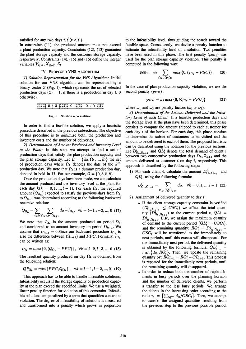
swap local search and insert local search. A swap local search procedure (Fig. 2) is based on

customer interchanging between every pair of routes. For a given solution represented by the set of routes R = {Rl,R2, ... ,R,}, in which Rl is the set of customers served by vehicle m, a swap local search procedure performs all possible swap moves between customers. In each move, we select a customer in route Rm and exchange it with another customer in the same route or in another route

Rm,(m = 1, ... ,f;m' = 1, ... ,i).

Tnitial routes

Swap customers

Fig. 2. Swap local search procedure

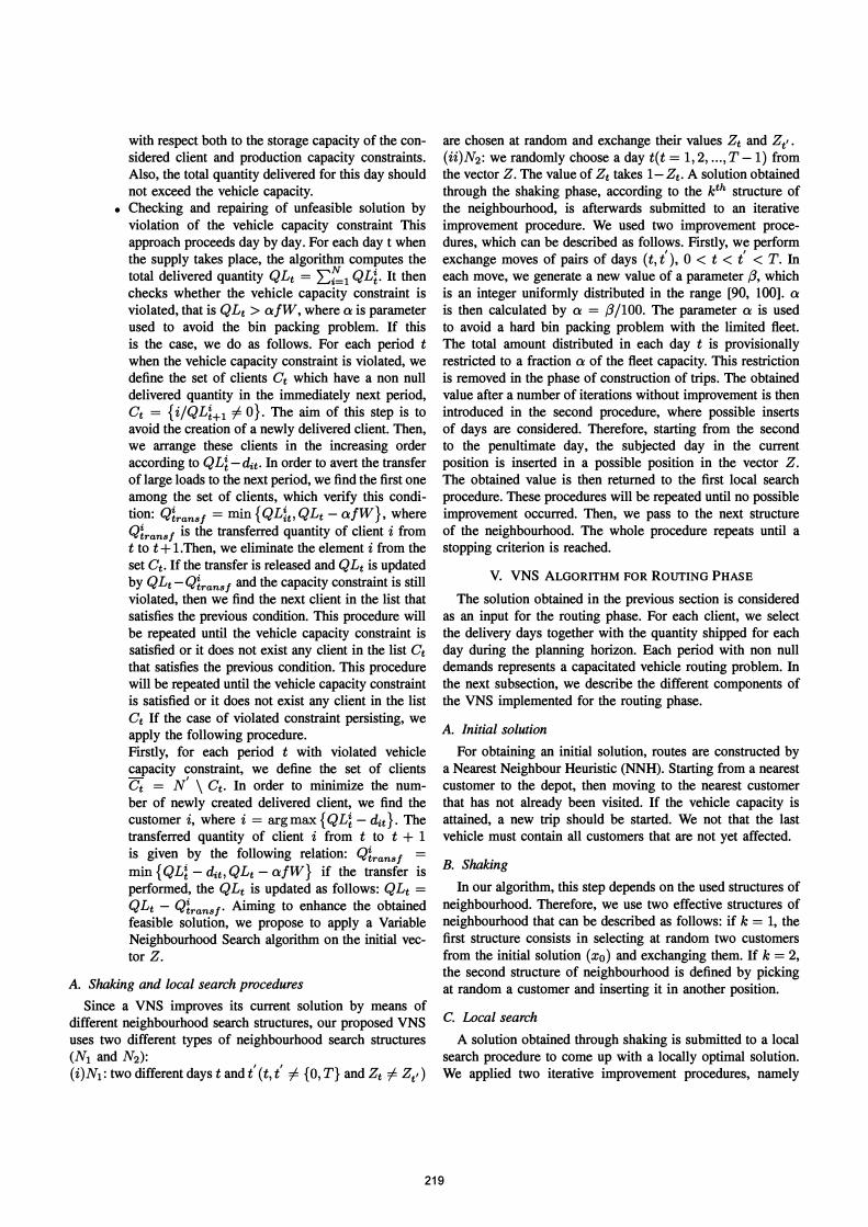
In insert local search procedure (Fig. 3), all possible insert moves of customers are considered. Starting from the first

candidate customer to the last one, the SUbjected customer in the current position in route Rm' (m # m ) is removed to another position in the same route or in another route. For each period, if the obtained solution (X2) is better than the initial solution (xo ) , then we replace (xo ) by (xd and return to the first structure of neighbourhood (k = 1), else we pass to the next neighbourhood structure (k = k + 1). If k = 2 and f (Xl) > f (X2), we pass to the next period. While the

Initial routes

Swap customers

._._._-- XI ._._._-@

Fig. 3. insert local search procedure

stopping criterion is not met, after terminating all periods, we can return to the first period and restart the previous steps. For each move or insertion of a client in another route, we verify the vehicle capacity constraint. In case of violating this constraint, the solution cost is typically augmented by the following penalty function:

pen3 = W3 L L max{O, (QL� - W)} (23)

tETiERt

where Rt denotes the set of routes in the period t and W3 is a penalty factor. After performing the shaking and the local

search procedures, the solution so obtained has to be compared to the incumbent solution in order to decide whether or not accepting it. The whole procedure is repeated until a stopping criterion is reached.

V I. IMPLEMENTATION AND EXPERIMENTAL RESULT

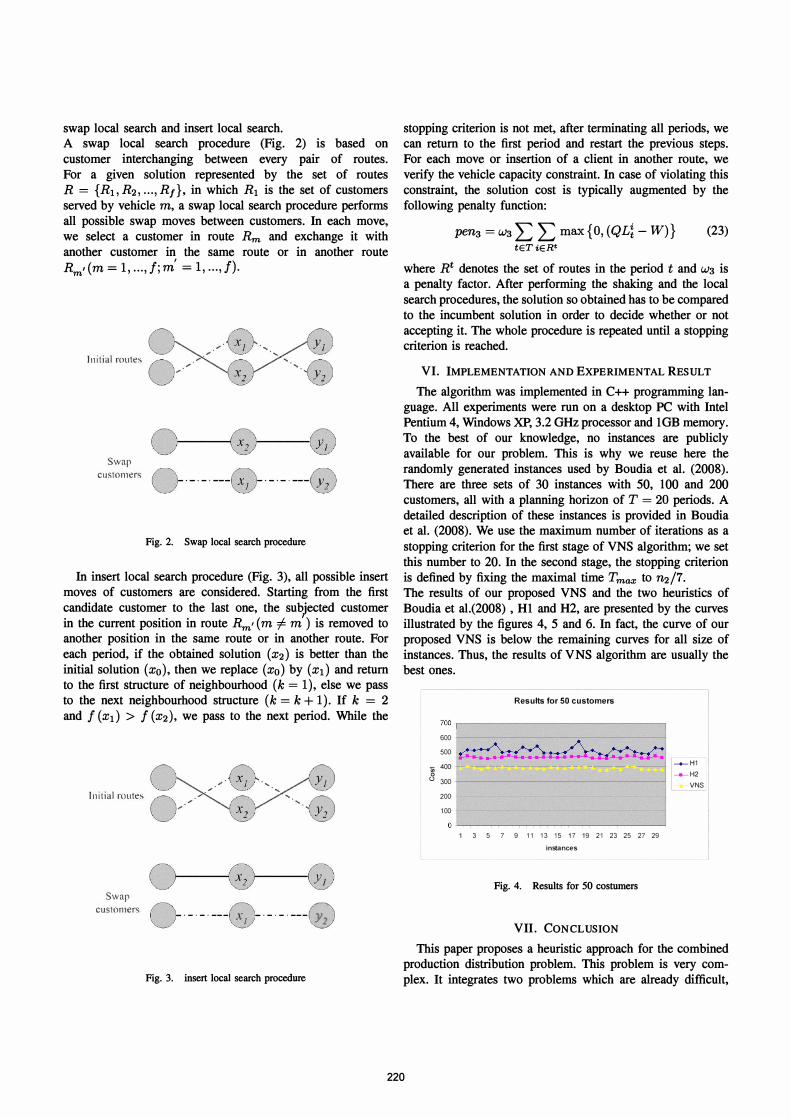
The algorithm was implemented in C++ programming lan­guage. All experiments were run on a desktop PC with Intel Pentium 4, Windows XP, 3.2 GHz processor and 1GB memory. To the best of our knowledge, no instances are publicly available for our problem. This is why we reuse here the randomly generated instances used by Boudia et al. (2008). There are three sets of 30 instances with 50, 100 and 200 customers, aU with a planning horizon of T = 20 periods. A detailed description of these instances is provided in Boudia et al. (2008). We use the maximum number of iterations as a

stopping criterion for the first stage of VNS algorithm; we set this number to 20. In the second stage, the stopping criterion is defined by fixing the maximal time T max to n2 /7. The results of our proposed VNS and the two heuristics of Boudia et al.(2008) , HI and H2, are presented by the curves illustrated by the figures 4, 5 and 6. In fact, the curve of our proposed VNS is below the remaining curves for all size of instances. Thus, the results of VNS algorithm are usually the best ones.

Results for 50 customers

700 � ________________________ � 600 500 �-' __ ����������� I

iii 400 o

u 300 200 100

1 3 5 7 9 11 13 15 17 19 21 23 25 27 29 instances

Fig. 4. Results for 50 costumers

V II. CONCLUSION

--+-H1 ____ H2

VNS

This paper proposes a heuristic approach for the combined production distribution problem. This problem is very com­plex. It integrates two problems which are already difficult,

220

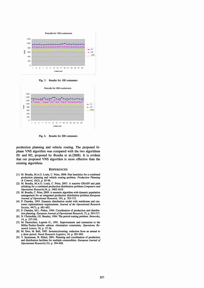
Results for 100 customers

1200 r--------------------------------, 1000 ................... I ••••••• � •••••••

;;; 8 600

400

200

1 3 5 7 9 11 13 15 17 19 21 23 25 27 29 instances

Fig. 5. Results for 100 costumers

Results for 200 customers

1600 r--------------------------------, 1400 1200 1000

§ 800 600 400 200

l ........... _�

1 3 5 7 9 11 13 15 17 19 21 23 25 27 29 instances

Fig. 6. Results for 200 costumers

--+-H1 ___ H2

VNS

--+-H1 ___ H2

VNS

production planning and vehicle routing. The proposed bi­phase VNS algorithm was compared with the two algorithms

HI and H2, proposed by Boudia et al.(2008). It is evident that our proposed VNS algorithm is more effective than the existing algorithms.

REFERENCES

[1] M. Boudia, M.A.O. Louly, c. Prins, 2008. Fast heuristics for a combined production planning and vehicle routing problem. Production Planning & Control, 19(2), p. 85-96.

[2] M. Boudia, M.A.O. Louly, C. Prins, 2007. A reactive GRASP and path relinking for a combined production-distribution problem. Computers and Operations Research,34, p. 3402-3419.

[3] M. Boudia, C. Prins, 2009. A memetic algorithm with dynamic population management for an integrated production distribution problem.European Journal of Operational Research, 195, p. 703-715.

[4] P. Chandra, 1993. Dynamic distribution model with warehouse and cus­tomer replenishment reqnirements. Journal of the Operational Research Society, 44(7), p. 681-692.

[5] P. Chandra, M.L. Fisher, 1994. Coordination of production and distribu­tion planning. European Journal of Operational Research, 72, p. 503-517.

[6] N. Christofide, J.E. Beasley, 1984. The period routing problem. Networks, 14, p. 237-256.

[7] M. Desrochers, Laporte G., 1991. Improvements and extensions to the Miller-Tucker-Zemlin subtour elimination constraints, Operations Re­search Letters, 10, p. 27-36.

[8] M. Dror, M. Ball, 1987. Inventory/routing: reduction from an annual to a short period. Naval Research Logistics, 34, p. 891-905.

[9] V. Jayaraman, H. Pirkul, 2001. Planning and coordination of production and distribution facilities for multiple commodities. European Journal of Operational Research,133, p. 394-408.

221