A 3-Step Math Heuristic for the Static Repositioning Problem in Bike-Sharing Systems

Transportation Research Part B 71 (2015) 230–247

Contents lists available at ScienceDirect

Transportation Research Part B

journal homepage: www.elsevier .com/ locate / t rb

A 3-step math heuristic for the static repositioning problemin bike-sharing systems

http://dx.doi.org/10.1016/j.trb.2014.10.0030191-2615/� 2014 Elsevier Ltd. All rights reserved.

⇑ Corresponding author.E-mail addresses: [email protected] (I.A. Forma), [email protected] (T. Raviv), [email protected] (M. Tzur).

Iris A. Forma a,b, Tal Raviv a,⇑, Michal Tzur a

a Industrial Engineering Department, Tel Aviv University, Tel Aviv, 6997801, Israelb Afeka College of Engineering, Bnei Ephraim 218, Tel Aviv, 6910717, Israel

a r t i c l e i n f o

Article history:Received 12 July 2014Received in revised form 6 October 2014Accepted 7 October 2014

Keywords:Bike sharing systemsMath heuristicsVehicle routing

a b s t r a c t

Over the last few years, bike-sharing systems have emerged as a new mode of transporta-tion in a large number of big cities worldwide. This new type of mobility mode is stilldeveloping, and many challenges associated with its operation are not well addressedyet. One such major challenge of bike-sharing systems is the need to respond to fluctuatingdemands for bicycles and for vacant lockers at each station, which directly influences theservice level provided to its users. This is done using dedicated repositioning vehicles (lighttrucks) that are routed through the stations, loading and unloading bicycles to/from them.Performing this operation during the night when the demand in the system is negligible isreferred to as the static repositioning problem. In this paper, we propose a 3-step mathemat-ical programming based heuristic for the static repositioning problem. In the first step,stations are clustered according to geographic as well as inventory (of bicycles) consider-ations. In the second step the repositioning vehicles are routed through the clusters whiletentative inventory decisions are made for each individual station. Finally, the originalrepositioning problem is solved with the restriction that traversal of the repositioning vehi-cles is allowed only between stations that belong to consecutive clusters according to theroutes determined in the previous step, or between stations of the same cluster. In the firststep the clusters are formed using a specialized saving heuristic. The last two steps are for-mulated as Mixed Integer Linear Programs and solved by a commercial solver. The methodwas tested on instances of up to 200 stations and three repositioning vehicles, and wasshown to outperform a previous method suggested in the literature for the same problem.

� 2014 Elsevier Ltd. All rights reserved.

1. Introduction

Bike-sharing systems offer a low cost and environmentally friendly mean of transportation for short travels. It can also beused as a complementary mode to other public transit such as buses, trams or subways. In order to provide high qualityservice, bicycles and vacant lockers should be available to the users of these systems when and where they are demanded.This can be achieved by repositioning the bicycles in the system according to forecasted demand rates for bicycles and lockersat the stations, using a dedicated fleet of light trucks. These trucks, referred to as repositioning vehicles, travel among thestations, where bicycles are loaded or unloaded subject to bicycle availability and capacity limitations at the repositioningvehicles and at the stations. When the repositioning is carried out during the day when the system is active, it is referred to

http://crossmark.crossref.org/dialog/?doi=10.1016/j.trb.2014.10.003&domain=pdf

http://dx.doi.org/10.1016/j.trb.2014.10.003

mailto:[email protected]



http://dx.doi.org/10.1016/j.trb.2014.10.003

http://www.sciencedirect.com/science/journal/01912615

http://www.elsevier.com/locate/trb

I.A. Forma et al. / Transportation Research Part B 71 (2015) 230–247 231

as dynamic repositioning and when it is carried out during the night when the demand for bicycles is negligible it is referredto as static repositioning.

In this paper we consider the static repositioning problem (SBRP), as defined in Raviv et al. (2013). In particular, the goal isto minimize a weighted sum of the expected number of unserved users (due to shortage of both bicycles and lockers) duringthe next working day, and the total traveling distance. The planning horizon of the repositioning operation is limited in time,typically five to six hours, to reflect the fact that it should be completed before dawn. Loading and unloading times ofbicycles at the stations are taken into account; in practice, the loading and unloading operation amounts to most of theworking time of the repositioning crew. Raviv et al. (2013) propose several Mixed Integer Linear Program formulationsfor the SBRP. Their numerical experiment shows that the formulation referred to as the arc-indexed (AI) is very effectivefor solving real life instances with up to 100 stations and two repositioning vehicles. In this paper we propose a 3-step mathheuristic that is based on a new clustering concept and on the AI formulation. We show that our heuristic produces solutionswith small optimality gaps for large instances.

In the first step of our heuristic, stations are clustered according to geographic as well as inventory (of bicycles) consid-erations. In the second step the repositioning vehicles are routed through the clusters while tentative inventory decisions aremade for each individual station. Finally, in the third step the exact routing of the repositioning vehicles is determined, alongwith the (possibly revised) number of bicycles to be loaded and unloaded at each station. The routing decisions are subject torestrictions imposed by the solution of the previous step.

The goal of the first step is to create clusters of stations that are geographically close together and that are likely to bevisited successively within the same route. Moreover, they are formed such that their requirements for loading andunloading bicycles are complementary. The purpose of the second step is to determine the set of clusters that are visitedby each repositioning vehicle and the sequence in which they are visited. These routing decisions are made together withsome preliminary inventory decisions that take into consideration the time needed for the loading and unloading operations.These inventory decisions are subject to refinement in the third step, in which the original repositioning problem is solvedwith restrictions on the traversal of the repositioning vehicles. Namely, traversal is allowed only between stations thatbelong to consecutive clusters according to the routes determined in the previous step, or between stations of the same clus-ter. Since in this step the assignment of stations to repositioning vehicles is already fixed, the repositioning problem is solvedfor each vehicle separately. The last two steps are formulated as Mixed Integer Linear Programs that are similar to the AIformulation introduced in Raviv et al. (2013), and solved using a commercial solver.

The applicability of the proposed method is numerically demonstrated by solving a variety of instances that are based onreal data. The results indicate that near optimal solutions of real life instances with up to 200 stations and three repositioningvehicles can be obtained. These results significantly outperform the results of applying the AI formulation on the originalproblem, in the same computational environment.

The contribution of this paper is in presenting a successful math-heuristic solution method to the SBRP, which is suitablefor large real life instances of the problem. Although our heuristic is based on decomposing the problem into smallersub-problems that are solved separately, our method is quite different from typical clustering approaches known in the lit-erature for vehicle routing problems, see Section 2. We believe that our new decomposition approach may be useful for otherrich vehicle routing problems.

The rest of the paper is organized as follows: in Section 2, we review the literature, describing related work from severalapplication areas. In Section 3, we formally state the SBRP and present some notation. In Section 4, we present our algorithmin detail, where a separate sub-section is dedicated to each of its three steps. In Section 5, we describe our numerical exper-iments, the results, and their analysis. Finally, in Section 6, we conclude and discuss possible extensions and directions forfurther research.

2. Literature review

Bike sharing systems rapidly gained popularity during the last decade, first in West Europe and East Asia and morerecently in North America. DeMaio and Meddin (2014) maintain a geographical database that describes the location andthe characteristic of all public bike-sharing systems around the world. Larsen (2013) reports that as of April 2013 more than500 cities host advanced bike-sharing systems with a combined fleet of more than half a million bicycles. Many cities are inthe process of planning and deploying new systems or extending existing ones.

Design and operation of bike sharing systems raised a set of new interesting problems to be addressed. First, the extentand the nature of the demand of a new bike-sharing system should be forecasted. Then, some strategic problems need to beaddressed. These include the coverage, capacity and density of the system. Next, the actual location of the stations and theircapacity should be designed. At a more tactical level, pricing and reservation policies should be determined by the operator.Finally, the day-to-day operation of the system requires rebalancing the system continuously in order to meet the demandfor bicycles and vacant lockers at the location and times desired by the users. While practitioners in the bike-sharing indus-try are already dealing with these challenging problems, with various levels of success, the scientific literature on the abovetopics is still relatively sparse. Below we describe the state of the art in the scientific literature.

Several studies try to estimate and forecast the demand in existing bike-sharing systems using data mining and classicalempirical methodologies. For some examples see Kaltenbrunner et al. (2010), Vogel et al. (2011), Côme et al. (2013) and

232 I.A. Forma et al. / Transportation Research Part B 71 (2015) 230–247

Rudloff and Lackner (2014). Lin and Yang (2011) address the combined problem of selecting optimal locations for bike-shar-ing stations and designing the bicycle paths network in a city so as to minimize the total travel costs of all users in the city.Romero et al. (2012) propose a bi-level optimization model for the optimal location of bike-sharing stations where the goal isto maximize the number of travelers that use the system. Chow and Sayarshad (2014) proposed a new framework to designtransportation networks in the presence of coexisting networks. The framework was applied to a bike-sharing system in thepresence of a coexisting transit system and was shown to result in a capacitated multicommodity flow problem. Shu et al.(2005) study the design and management of a stochastic vehicle-sharing system. Shu et al. (2013) develop a network flowmodel for a system in which the flow is determined by the random demand of the travelers. They examine the effect of redis-tribution of bicycles in the network and the capacity of the stations on the flow in the system. Nair et al. (2013) studied theVélib’ system in Paris from several aspects, including system characteristics, utilization patterns, the connection betweenpublic transit and bicycle-sharing systems, and flow imbalances between stations. Rudloff and Lackner (2014) build a sta-tistical model for the demand for bikes and lockers by studying the influence of weather and full/empty neighboring stationson demand.

In order to cope with the inherent asymmetry and stochasticity of trips in the system, two general methods were pro-posed for diverting the demand towards more balanced patterns. Waserhole and Jost (2015) present a dynamic pricingmechanism that forces a balanced demand and hence save the need for repositioning altogether. Such an approach clearlycomes at the cost of reducing the level of service provided to the users of the system but nevertheless seems the only viablealternative to balancing a car sharing system where repositioning is too expensive. Fricker and Gast (2015) use mean-fieldapproximation to analyze the effect of a simple incentive mechanism on the service provided by the system and the optimalfleet size. Kaspi et al. (2014a, 2014b) explore operational policies in which the users of the system reserve lockers at thedestination upon the beginning of their journey. Trips can be denied or the destination can be slightly diverted if no vacantlockers are expected to be available at the true destination.

Many studies on bike-sharing systems deal with some variants of the static repositioning problem, which is also the topicof this work. Some authors refer to the same class of problems as rebalancing problems but since, as mentioned above, abalance in the system can also be achieved by pricing incentives and reservations, we prefer the term repositioning. Notethat the static repositioning problem is not uniquely defined since various studies make different modeling assumptions.Most of the authors viewed the problem as an extension of the single commodity many-to-many pickup and delivery prob-lem introduced by Hernández-Pérez and Salazar-González (2004). In particular, most studies consider the total distancetraveled by the repositioning vehicles, as the objective function. Berbeglia et al. (2007) provide a survey and classificationof pickup and delivery problems; see also the discussion below regarding the differences between the problem consideredhere and pickup and delivery problems.

Chemla et al. (2013a) propose a math-heuristic for the single vehicle version of the problem, assuming each station can bevisited more than once. Their algorithm is based on a solution of a relaxation of the problem that is solved by a branch-and-cut procedure. The objective function is to find a route that minimizes the total traveling distance. Erdogan et al. (2013)extend the pickup and delivery model to allow the final inventory at each node to be within a prescribed interval insteadof at a unique level. This model reflects the idea that there are some degrees of flexibility in the desired number of bicyclesat each station at the end of the static repositioning operation. They present a branch-and-cut algorithm and a Benderdecomposition that allows solving instances with up to 50 stations. Schuijbroek et al. (2013) study the static repositioningproblem with a service level constraint. Similarly to Erdogan et al. (2013) they assume that the service level constraint is metwhen the desired inventory level at the end of the repositioning operation is within a given interval. They present a queuingmodel that allows calculating the required interval given the desired service level. Next, the paper introduces a cluster-firstroute-second algorithm where the clustering problem is solved by a heuristic that is based on the maximum star approxi-mation of the TSP. The routing problem of each repositioning vehicle is then formulated as an integer program and solved bya commercial solver. Rainer-Harbach et al. (2013) and Raidl et al. (2013) present variable neighborhood search heuristics fora variant of the static repositioning problem that take the loading and unloading times into account.

Contrary to the approach of all the above studies, we believe that the desired number (or range) of bicycles at the stationsafter the static repositioning operation is completed should constitute a soft constraint, expressed as a penalty in theobjective function. From the operator’s point of view, the target inventory levels of bicycles are only idealistic goals to aspireto.

Raviv et al. (2013), based on Forma et al. (2010) further extend the many-to-many pickup and delivery problem intro-duced by Hernández-Pérez and Salazar-González (2004) by including the following characteristics that are not consideredby other studies: (a) the objective function incorporates a service level component directly, that is, the goal is to minimizea weighted sum of the expected number of un-served users (due to shortage of both bicycles and lockers) during the nextworking day, and the total traveling distance. The former part is calculated based on Raviv and Kolka (2013); (b) the planninghorizon of the repositioning operation is limited in time; (c) the loading and unloading times of bicycles at the stations aretaken into account. Near optimal solutions were reported for instances created based on the demand of actual systems withup to 104 stations and two vehicles, but as shown in this study, this marks the limits of the model size that can be solvedwith a reasonable optimality gap subject to a reasonable computing time constraint.

The solution method presented in this paper is built to solve the problem under the assumptions presented in Raviv et al.(2013) even though it can be easily adapted to the other optimization models presented in the literature. In the current studywe significantly increase the size of the problem instances that can be solved to near optimality.


Dynamic repositioning is much more intricate to manage because it incorporates a scheduling component derived fromthe users’ activity during the operation, together with a routing component. Contardo et al. (2012) assume dynamicdeterministic demand and formulate an optimization model to route a single vehicle that moves bicycles between stationsso as to minimize the number of shortage events. They propose a decomposition scheme that allows obtaining a solutionwith a reasonable optimality gap for instances with up 100 stations and 60 discretized periods, in ten minutes. Pessachet al. (2014) use a formulation that is similar to the time-indexed formulation of Raviv et al. (2013) within a rolling horizonframework in order to heuristically solve the actual stochastic and dynamic repositioning problem. Their method was shownto outperform a variety of heuristic method based on dispatching rules, including some of those used by practitioners.Chemla et al. (2013b) and Pfrommer et al. (2014) propose methods for dynamic rebalancing of the system that utilize bothpricing incentives and repositioning. Kloimüllner et al. (2014) suggest solving the dynamic balancing problem by greedy andPILOT construction heuristics, as well as variable neighborhood search and GRASP improvement heuristics.

As mentioned above, Schuijbroek et al. (2013) present a heuristic algorithm to the repositioning (rebalancing) problemthat can be classified as a cluster-first route-second approach, which is a quite prevalent approach in solving variousmulti-vehicle routing problems. It is based on the idea of building clusters of nodes/customers first, and then solving a seriesof independent single-vehicle TSP (or other routing) problems, one for each cluster. Early algorithms in this class include, forexample, the sweep heuristic by Gillett and Miller (1974) and the well-known heuristic of Fisher and Jaikumar (1981), whichuses the generalized assignment problem to create the clusters. A review of classical heuristics approaches can be found inLaporte and Semet (2002).

While our heuristic also builds clusters first and then constructs routes, it is quite different from the above literature. Themain difference is that a vehicle/route according to our approach travels through a sequence of clusters, whereas a vehicle/route according to the cluster-first route-second approach travels through a single cluster. The purpose of creating clusters inour heuristic is to reduce the network size, so that routing of multiple vehicles can be performed on the reduced network; inthe cluster-first route-second approach, the clusters are created in order to decompose the network so that a single vehicleserves each of them. We are not aware of other heuristic approaches that similarly to ours, reduce the network size in such amanner.

Battarra et al. (2014) studied the clustered vehicle routing problem (CluVRP), where the customers are clustered into pre-defined clusters, so that a vehicle visiting one customer in the cluster must visit all the remaining customers in the clusterbefore leaving it. Although this is similar to our heuristic in the fact that a vehicle visits several clusters, there are two maindifferences between the routing decisions of the CluVRP problem and ours: (i) in the CluVRP problem, the clusters of cus-tomers are given as part of the problem’s input, while in our problem they are created as part of the solution procedurein order to reduce the complexity of the problem; (ii) in the CluVRP problem, all nodes must be visited, while in our problemit is not a requirement; Other differences between the problems clearly exist, as the operation performed in our reposition-ing problem is quite more involved than supplying a given quantity to the customers, as in the CluVRP. Baldacci et al. (2010)introduce the generalized vehicle routing problem (GVRP), in which the clusters are also pre-defined. Each customer has anon-negative demand and a given number of vehicles must visit exactly one customer per cluster, such that the total costis minimized, and the routes obey capacity and time constraints. It is demonstrated that the GVRP provides a usefulmodeling framework for a wide variety of routing applications.

In conclusion, our 3-step algorithm advances the literature on repositioning problems and forms a practical approach formedium-large bike-sharing systems. Moreover, it presents a new type of decomposition method for a variety of vehiclerouting and inventory routing problems.

3. Problem definition

The SBRP addressed in this paper was first introduced by Raviv et al. (2013). For the sake of completeness we restate thisproblem here. Their arc-indexed formulation, which is used in this paper, is given in Appendix A.

The input of the SBRP consists of a set of stations, N, and a depot where all the repositioning vehicles are initially located.The set of the stations and the depot together are referred to as N0 where the depot is indexed by 0. Each station i e N is char-acterized by:

� Capacity ci, which is the maximum possible number of bicycles that it may store.� Initial bicycle inventory, s0

i .� Penalty function, fi(s), which represents the expected shortage of bicycles and lockers incurred by users in the station dur-

ing the next day as a function of the inventory at the station after the repositioning is carried out. Let fi(s) =1 for valuesout of the domain {0, . . ., ci}. Raviv and Kolka (2013) show how to calculate this function based on a demand forecast forthe station and prove its convexity. However any penalty function can be used as long as it is convex and separablebetween stations.

The depot may have its own capacity and initial inventory but these are typically assumed to be non-binding. The depotfaces no demand and hence incurs no penalty.


In addition, the input consists of:

� A set of vehicles V. Each vehicle has capacity kv.� The total time allocated for static repositioning, T. Typically, 5–6 h during the night.� The time L (resp., U) needed for the loading (resp., unloading) operation of each bicycle to (resp., from) the vehicle,

typically 1–2 min.� Vehicle driving time matrix, with elements tij between each pair of stations i and j, including the depot.� A weight, a, of the travel cost per time unit in the objective function. Without loss of generality, the weight of the

expected number of unserved users in the objective function is set to one.

In particular, the goal is to minimize a weighted sum of the expected number of unserved users (due to shortage of bothbicycles and lockers) during the next working day, and the total traveling distance. A solution of the problem constitute aroute for each vehicle that starts and ends at the depot, along with decisions on the number of bicycles to load/unload ateach station along the route, while satisfying the time constraint. The objective is to minimize a weighted sum of the penaltyfunction over all stations and the total travel cost of all the vehicles.

Let s�i be the inventory level at station i that minimizes fi(s). Clearly,P

if iðs�i Þ is a lower bound on the value of the objectivefunction of the above problem. We refer to s�i as the ideal inventory level of station i and to a solution that achieves the idealinventory level at all stations as an ideal solution. Due to the time limitation, T, it is generally infeasible to achieve an idealsolution. Moreover, even if an ideal solution is feasible, it is generally sub-optimal due to the travel cost component in theobjective function. Therefore, in general, the optimal solution differs from the ideal solution.

4. A 3-step heuristic approach

Our proposed algorithm is composed of three steps: first, stations are clustered according to geographic and inventoryconsiderations. Then, the vehicles are routed through the clusters while inventory decisions are made for each individualstation separately. Finally, the original static repositioning problem is solved for all stations, but traversal of the vehiclesis allowed only between stations of the same cluster or stations that belong to two consecutive clusters, according to thedecisions made in the previous step. These steps are described next.

In this section we use the following definitions: Given a cluster of stations I, let its initial inventory, denoted by S0I , be the

sum of its stations’ initial inventories (i.e., before repositioning), and its capacity, denoted by CI, be the sum of its stations’capacities. That is:

S0I ¼

Xi2I

s0i ð1Þ

CI ¼Xi2I

ci ð2Þ

4.1. Step 1: A saving heuristic for building the clusters

The purpose of the first step is to create clusters of stations in order to solve a repositioning problem on the reduced net-work, whose nodes would refer to clusters. Each cluster may include several stations, although a cluster of a single station isalso possible.

To create clusters such that the repositioning solution on the reduced network will serve the objective of the originalproblem, two issues need to be considered: the geographic location and the initial inventory. Since in the next steps ofthe algorithm, the stations are visited cluster by cluster, we would like the stations in a given cluster to be geographicallyclose to each other. Therefore, we limit the diameter of each cluster, i.e., the maximal distance (in terms of travel time)between stations that belong to the cluster. The maximal diameter allowed is denoted by D. Since as D decreases, we expectthe number of clusters to increase, the value of D is determined to be as low as possible such that the repositioning problemon the reduced network can still be solved in Step 2 in a reasonable amount of time.

The second issue to consider is the initial inventory of the clusters, which determine their costs. We define the total costof a cluster, FI(S), as the expected number of shortages that will be incurred in its stations when an inventory of S bicycles isarranged in the stations of cluster I in the best possible way, i.e., so as to minimize the sum of the expected number of short-ages in all of its stations. This definition is motivated by the fact that the stations of a cluster are visited by the same vehicle,which can easily transfer bicycles between them. For example, if we include in a certain cluster only stations in which theinventory level is lower than their ideal levels, transferring bicycles between these stations can not improve the service pro-vided by these stations significantly. On the other hand, if the inventory of some stations is higher than their ideal level, andof others is lower, then transferring bicycles between stations within this cluster can be more beneficial. In the former (lat-ter) case the cluster’s cost would be high (low).

FI(S) is formally defined by the following mathematical program:

FIðSÞ ¼ minsi :i2I

Xi2I

f iðsiÞ ð3Þ


s.t:
Xi2I
si ¼ S ð4Þ

In the above optimization problem, the decision variables are si ("i e I). The variable si denotes the inventory level at sta-tion i after distributing S bicycles among the stations of the cluster. Note that in the solution obtained, 0 6 si 6 ci"i since bydefinition, fi(si) =1 for si > ci or si < 0. We also remark that this distribution is not actually performed, it is determined onlyfor the sake of computing the value of FI(S). Later in this section we show how program (3), (4) can be efficiently solved.

We are now ready to formulate the clustering problem. A valid cluster has a diameter no larger than D. The objective func-tion, to be minimized, consists of two components: the number of clusters, and the sum of the expected costs of the clusters.Let I1, . . ., Im be a partition of the stations into m clusters. Then, finding the optimal partition is represented by the followingmathematical program, where m and I1, . . ., Im are the decision variables:

minm;I1 ;::;Im

mþ bXm

k¼1

FIkðS0

IkÞ

( )ð5Þ

s.t:

tij 6 D 8i; j 2 Ik; k ¼ 1; . . . ;m ð6Þ

Note that the two terms of the objective function (5) are expressed in different units: the first is the number of clustersand the second is a cost. Therefore, we multiply the second term by a scaling parameter b. We explain later how to choosethe value of b. Constraints (6) assure that the diameter constraint is satisfied, i.e., stations assigned to the same cluster areclose geographically. It is possible to formulate (5), (6) as an integer programming model. However, solving it exactly is com-putationally intractable and hence we devised a saving heuristic to solve it.

Our saving algorithm is based on two observations presented and proved in Lemma 1 and Lemma 2 below. In Lemma 1,we show how the cost function FI(S) can be efficiently evaluated and in Lemma 2 we prove that combining two clustersalways saves costs.

The following lemma demonstrates that the optimization problem (3), (4) is easily solved to optimality by a greedy pro-cedure. Such a procedure assigns the S units one by one, where each unit is assigned to the station where its contribution tothe objective function is minimal.

Lemma 1. Problem (3), (4) that finds the cost of a cluster can be solved by the following recursive procedure:Let ~siðI; SÞ ("i e I) be the optimal solution of (3), (4) for given I and S. Then,

FIðSþ 1Þ ¼ minj2I:~sjðI;SÞ<cj

ff jð~sjðI; SÞ þ 1Þ þXi–j

f ið~siðI; SÞÞg ð7Þ

~siðI;0Þ ¼ 0 8i;8I ð8Þ

Proof. The proof is by induction on the value of S. Clearly (8) holds. For S = 1, the solution must assign one unit to one of thestations. According to (7), the unit would be assigned to the station whose contribution to the objective function is minimal(note that the contribution can be negative), which is clearly the optimal solution for this case.

Now, define Di (s) � fi(s) � fi(s � 1). The convexity of the integer valued function fi( � ) implies that Di (1), Di (2), Di (3), . . .

is increasing. The relation (7) can be rewritten as

FIðSþ 1Þ ¼minj2IfDjð~sjðI; SÞ þ 1Þg þ

Xi

f ið~siðI; SÞÞ ð9Þ

Now, we assume that the optimal solution for S was obtained by recursively applying (9), and we claim that the optimalsolution for S + 1 is also obtained by (9). To prove that, let k ¼ argminj2IfDjð~sjðI; SÞ þ 1Þg. That is, Dkð~skðI; SÞ þ 1Þ 6Djð~sjðI; SÞ þ 1Þ "j – k.

Next we will show that: (a) ~skðI; Sþ 1Þ 6 ~skðI; SÞ þ 1; (b) ~skðI; Sþ 1ÞP ~skðI; SÞ þ 1. (a) and (b) imply that~skðI; Sþ 1Þ ¼ ~skðI; SÞ þ 1 and therefore ~sjðI; Sþ 1Þ ¼ ~sjðI; SÞ 8 j–k.

Part (a) is true since any increase of ~skðI; Sþ 1Þ beyond ~skðI; SÞ þ 1 would imply decreasing ~skðI; Sþ 1Þ in some otherstation(s) j – k. However, due to the convexity of all fj(.) functions and the procedure in (9) that implyDkð~skðI; SÞ þ lÞP Djð~sjðI; SÞ � pÞ "j – k for any number of units l P 2 and p P 1, such a solution cannot be optimal.

Part (b) is true since if ~skðI; Sþ 1Þ is not increased beyond ~skðI; SÞ, then ~sjðI; Sþ 1Þ for at least one other station j – k must beincreased. However, Dkð~skðI; SÞ þ 1Þ 6 Djð~sjðI; SÞ þ pÞ for any number of units p P 1. Thus, such a solution cannot be optimal.

We conclude that ~skðI; Sþ 1Þ ¼ ~skðI; SÞ þ 1 and ~sjðI; Sþ 1Þ ¼ ~sjðI; SÞ "j – k, by the induction assumption. This implies that(7) is satisfied. h


Consider now fixed values of initial inventories in the stations, ðs01; . . . ; s0

nÞ, and recall that S0I ¼

Pi2Is

0i . In order to calculate

the value of FIðS0I Þ, the minimization of (7) needs to be carried out for all S ¼ 1; . . . ; S0

I . Although the complexity of this pro-

cedure is OðS0I Þ which is pseudo-polynomial, we note that the value S0

I of a typical cluster would be in the range of tens or afew hundred at most, therefore it can be solved very quickly. When solving this problem for each value of S from zero up to CI

units, we obtain a full characterization of the FI( � ) function. An immediate corollary of Lemma 1 is that this function is con-vex. The collection of functions FI( � ) also satisfies the following property:

Lemma 2. Given disjoint clusters I and J, FI[JðS0I þ S0

J Þ 6 FIðS0I Þ þ FJðS0

J Þ.

Proof. The proposition is proved by,

FI[JðS0I þ S0

J Þ ¼Xi2I[J

f ið~siðI [ J; S0I þ S0

J ÞÞ 6Xi2I

f ið~siðI; S0I ÞÞ þ

Xi2J

f ið~siðJ; S0J ÞÞ ¼ FIðS0

I Þ þ FJðS0J Þ:

The inequality above is due to the fact that in the combined cluster, one possible solution for the inventory level at thestations, is to arrange it in the same way as it is done in the separate clusters. However, additional arrangements are possible,which may reduce the cost of the combined cluster. h

Our saving heuristic algorithm for the clustering problem, (5), (6), is based on a saving function, denoted by Fsaving(I, J),which represents the saving in the objective function value (5) when combining two distinct clusters I and J into onenew cluster. This function is defined for any pair of clusters I and J, whose stations satisfy the distance constraint (6). Thesaving function is calculated as follows:

For all I and J such that (6) is satisfied, i.e., tij 6 D "i e I, j e J,

FsavingðI; JÞ ¼ 1þ b½FIðS0I Þ þ FJðS0

J Þ � FI[JðS0I þ S0

J Þ� ð10Þ

The expression in (10) represents the saving because when combining two clusters, the number of clusters in the solutionis reduced by one, and a joint cost FI[JðS0

I þ S0J Þ is incurred instead of the sum of the separate costs FIðS0

I Þ þ FJðS0J Þ, with the

respective weight.The saving heuristic iterations are performed as follows: Initially, each cluster is represented by a single station and the

saving is calculated according to (10) for each pair of clusters whose stations comply with the traveling distance constraint,(6). The pair of clusters with the maximum saving is chosen to be combined into one cluster. The saving and the compliancewith the distance constraint is re-calculated for all pairs that include the newly created cluster, and the process is repeateduntil no pair of clusters satisfies constraint (6). In fact, since by Lemma 2, FIðS0

I Þ þ FJðS0J Þ � FI[JðS0

I þ S0J ÞP 0, both terms of (10)

are always non-negative for any pair of clusters. Moreover, the first term of (10) is constant (and equals one) for any pair of Iand J, therefore the pair that is selected to be combined is simply the one that maximizes FIðS0

I Þ þ FJðS0J Þ � FI[JðS0

I þ S0J Þ. Inter-

estingly, the value of b is irrelevant for this proposed heuristic and we believe that the value of this parameter admits veryminor effect on the optimal solution of the clustering problem. Note that the proposed saving heuristic is inspired by the ideaof the saving heuristic for the vehicle routing problem, introduced by Clarke and Wright (1964).

4.2. Step 2: The repositioning problem on the clusters

In the second step, the routes of the vehicles through the clusters are determined, along with tentative decisions on theamount of bicycles to be loaded or unloaded at each station (in the visited clusters). The routing within each cluster is ignored,so that the operations are planned as if all the stations of each cluster are at exactly the same location. For simplicity, we chosethis location to be at the station that is closest to the centroid of the cluster. Note that the difficulty in solving large-scale repo-sitioning problems stems from the routing decisions and not from the inventory decisions. Therefore we allow at this stageperforming detailed (for each station) inventory decisions while the routing decisions are made only at the cluster level.

We formulate the problem of this step as a mixed integer linear model by adapting the arc-indexed (AI) formulation ofRaviv et al. (2013) to this reduced and relaxed version of the problem. We include the revised model in Appendix B. Since thenumber of clusters is significantly smaller than the number of stations in the original problem, it is possible to solve thismodel using a commercial solver for fairly large instances.

In order to allow decomposition of the problem to separate single vehicle problems at the next step, additionalconstraints were imposed on the model at this step. Namely, each cluster can be served by at most one vehicle. This is imple-mented by constraint (33), see Appendix B. While this additional constraint may eliminate some good solutions of the prob-lem, it simplifies Step 3 greatly and thus allows solving larger instances of the problem with smaller optimality gaps underlimited computational resources.

The results obtained from the second step do not correspond with a feasible solution to the original problem, since thetravel times between stations belonging to the same cluster are ignored. The purpose of this step is merely to determine theorder in which the clusters will be visited by each vehicle in Step 3 of the algorithm. The inventory decisions made at Step 2are only tentative and are included in the model only to facilitate reasonable routing decisions between the clusters.


4.3. Step 3: Obtaining the solution

In this step, the solution of the problem is obtained. The input to this step includes the routing decisions obtained in Step2, that specify which clusters were visited by each vehicle and in what order. Note that since at Step 2 we allow each clusterto be visited by a single vehicle, the sets of clusters that are visited by each vehicle are disjoint. This creates separateproblems, one for each vehicle.

For each vehicle, the constraints imposed by Step 2’s decisions specify which clusters will be visited by the vehicle and inwhat order. Contrary to Step 2, the routing decision variables between stations that belong to the same cluster are alsoincluded in the model, but now this poses lesser computational difficulty due to the separation between the vehicles andthe smaller number of stations associated with each vehicle’s problem. Finally, inventory decisions for all stations are madeaccording to the actual (original) constraints of the problem.

Next we define the separate network for each vehicle, on which the repositioning problem is solved. The problem for eachvehicle v e V is defined on a directed graph Dv = (Nv [ {0}, Av). The node set Nv is the set of all stations that belong to clustersvisited by vehicle v according to Step 2. The depot is added to this node set. The set of arcs, Av, consists of four categories:

1. All arcs between nodes in Nv that represent stations in the same cluster. That is, if I is a cluster visited by vehicle v in thesolution of Step 2, then for all pairs of nodes i, j e I, arc (i, j) is in Av.

2. All arcs between ordered pairs of nodes in Nv that belong to two consecutive clusters in the routing of vehicle v inStep 2. That is, if vehicle v travels from cluster I to cluster J, and i e I and j e J are stations in those clusters, then arc(i, j) is in Av.

3. All arcs between the depot node and the nodes that belong to the first visited cluster in the route of vehicle v inStep 2.

4. All arcs between nodes that belong to the last visited cluster in the route of vehicle v in Step 2, to the depotnode.

The above definition of the set Av for vehicle v reflects our belief that the route generated between the clusters of thisvehicle, provide good guidelines for the final route. In particular, the sequence of traversing the clusters is kept almostunchanged but more flexibility is added by allowing traveling within the clusters and between any two stations ofconsecutive clusters. Moreover, loading and unloading decisions are reconsidered and finalized at this stage. The problemsare solved sequentially, one problem for each vehicle, since the networks of different vehicles are completely disjoint. Anexample that demonstrates the steps of the algorithm is presented in Fig. 1.

In Fig. 1, the clusters created in Step 1 are circled and the stations of each cluster are denoted by a different shape. InFig. 1a, we present the route of each vehicle through the clusters assigned to it in Step 2. The location of each cluster isrepresented by a single station that is closest to its centroid. In Fig. 1b, we present the final route of each vehicle throughthe stations it visits.

5. Numerical experiments

In this section, we present results that were obtained when solving instances of practical size with the 3-step heuristicdescribed in Section 4. We compare the results to those obtained by solving the AI formulation of the original network, usingCPLEX. We start by describing and analyzing instances that are based on data from the Vélib system (in Paris). We used theactual locations of some 200 Vélib stations located in the first through the fifth arrondissements. The input of our instances isavailable online at: http://www.eng.tau.ac.il/~talraviv/Publications/.

(a) (b)

Step 1: Creating the clusters Step 2: Routing the vehicles through them

Step 3: Routing each vehicle through the stations in the sequence of clusters determined in Step 2.

Fig. 1. Example of the solutions obtained by the 3-step algorithm.

http://www.eng.tau.ac.il/~talraviv/Publications/


We conducted an experiment with all the combinations of the following parameter values:

� Number of stations – 75, 100, 125, 150 and 200 stations, where the smaller instances are subsets of the larger ones.� Penalty function – representing the expected number of shortages function (fi(.) for station i), based on a fictitious (but

likely representative) demand pattern. The penalty functions were constructed as follows: The stations of the system weredivided into three types, namely, (1) residential area stations where the demand for bicycles is high in the morning and thedemand for lockers is high in the afternoon; (2) Business area stations with complementary pattern of demand; (3) ‘‘tour-istic’’ stations where the intensity of the demand for bicycles and lockers behave similarly throughout the day. The penaltyfunctions were calculated using the method of Raviv and Kolka (2013) based on the actual capacity of each station.� Workload (light, real, heavy) – the initial inventory levels at the stations influence the amount of work necessary in order

to reach their ideal inventory levels. The further the initial inventory level of a station is from its ideal level, the morework is necessary. That is, the number of bicycles to load/unload to/from the station is higher. Therefore, we test threedifferent cases of initial inventories called: ‘‘light ‘‘, ‘‘real’’ and ‘‘heavy’’ referring to different workloads. For the ‘‘light’’case we generated initial inventories from a normal distribution with mean that corresponds to the ideal inventoryand a standard deviation that equals to 0.2ci. In the ‘‘heavy’’ case, the standard deviation is equal to 0.6ci. In this waywe generate data with a higher expected workload. The ‘‘real’’ case corresponds to real initial inventories that wereobserved in the system at midnight on a random day.� Number of vehicles – two and three vehicles.� Total time allocated to repositioning – 5 h (18,000 s).� a, the weight of the operating/travel costs per second relative to an expected shortage of one unit – a value of 1/900 was

used. This means that traveling 900 s (=15 min) is equivalent (in cost) to an expected shortage of one user.

The travel time matrix was calculated based on the L1 (Manhattan) metric. The loading and unloading times were set tobe one minute/bicycle. The vehicle’s capacity was set to 25 bicycles, which is the capacity of the light trucks used by Vélib.The location of the depot was selected to correspond to the location of station number one, situated in the 1st quarter. Thecapacity and the initial inventory of the depot were set to be large enough so that they were not binding. The dataset for ourbenchmark problems is available from the authors upon request.

After some tuning, we set the parameter that defines the maximal distance between stations in the same cluster, D, to be800 s.

The saving heuristic used for the first step of our algorithm is implemented by a code computed with MATLAB. We imple-mented the second and third steps using IBM-Ilog OPL, and solved the above instances using IBM-Ilog CPLEX 12.3 on an Inteli7 2600 @ 3.4 GHz with 16 GB of RAM. In all our experiments, we used CPLEX’s default settings.

While the saving heuristic of Step 1 took few seconds to run and the model of Step 3 was solved by CPLEX in a very shorttime as well (up to 42 s for the hardest instances), we could not solve the model of Step 2 for the larger instances in areasonable time. Therefore, we set a time limit of one hour and used the best integer solution obtained by this time. In realscenarios one hour is approximately the time that can be allotted since the problem should be solved before the reposition-ing vehicles start their duties but after the state of the stations is revealed.

For the sake of benchmarking the 3-step algorithm we also solved the AI formulation subject to the same time limitationof one hour. Table 5, which contains detailed results of our experiments with both the 3-step algorithm and the AI formu-lation, is provided in Appendix C. In the rest of this section we summarize various aspects of these results and discuss theirimplications.

The outcome of Step 1 for each instance was a set of clusters where the average number of stations per cluster was aboutfour. Therefore, the dimension of the routing problem solved at Step 2 decreased significantly.

In order to explore the limits of Step 2 we report in Table 1 on the quality of the results of this step in terms of optimalitygaps obtained within one hour. For the smaller instances that were solved to optimality in less than one hour we report onthe solution time in seconds, instead. The first two columns of the table describe the characteristics of the instances in terms

Table 1Relative optimality gap and solution time for Step 2.

Stations Vehicles Relative Optimality Gap Step 2 (%) Solution time Step 2 (s)

Light Real Heavy Light Real Heavy

75 2 * * * 108 91 1103 * * 0.28 114 188 3600

100 2 * * * 1154 237 11173 0.11 * 1.59 3600 614 3600

125 2 * * * 2119 727 4233 0.65 0.12 1.78 3600 3600 3600

150 2 0.34 * 0.31 3600 1684 36003 1.10 0.84 1.57 3600 3600 3600

200 2 1.05 2.16 0.99 3600 3600 36003 2.52 1.77 2.12 3600 3600 3600


of number of stations and number of vehicles. The next three columns present the relative optimality gaps for the light, realand heavy workloads. The relative optimality gap, as calculated by CPLEX, is defined as follows:

Table 2Relative

Stati

75

100

125

150

200

Relative Optimality Gap ¼ Solution value� Lower boundSolution value

The optimality gap is calculated relative to the lower bound obtained from the MILP solver for the problem solved in Step 2.Note that, strictly speaking, this is not a valid lower bound for the original problem because the route between the centers ofthe clusters may be, in some rare cases, longer than the route between the stations that are actually served. This may occur, ifnot all the stations of the visited clusters are served in the optimal solution. A valid lower bound for the original problem ispresented below. An asterisk (⁄) is used to denote instances that were solved within the CPLEX default optimality toleranceof 0.01%. The three rightmost columns present the solution time in seconds. A value of 3600 s is reported for instances thatcould not be solved to optimality within one hour.

We observe that while most of the larger instances could not be solved to optimality within the allotted hour, the opti-mality gaps of all tested problems are not larger than 2.52%. Since Step 2 is the most computationally demanding componentof our heuristic, these results imply its applicability to large problems. As expected, the optimality gap and solving timeincrease as the network size and the number of vehicles increases. However, these values are less sensitive to the workload,whereas the real workload is the easiest to solve in most cases.

In Table 2 we present the relative optimality gaps obtained for the 3-step algorithm and the AI formulation. The gaps forboth solution methods are defined relative to a valid lower bound of the original problem, obtained from the MILP solver forthe AI formulation. The structure of the table is identical to that of Table 1.

We observe from Table 2 that the instances with real workload are solved by the 3-step algorithm with a small optimalitygap, between 0.95% and 5.11%. In all the harder instances, the optimality gaps of the solutions obtained by the 3-stepalgorithm are significantly smaller than those obtained by the AI formulation. In fact, the AI formulation could not obtaina feasible solution for 17 out of the 30 test instances. The optimality gap of these instances is reported in the table as‘‘�’’. The AI formulation outperformed the 3-step algorithm only in two instances, with 75 stations and light workload.The optimality gaps of the 3-step algorithm are greatly affected by the workload, with higher optimality gaps for heavierworkload. Interestingly, the workload obtained from observing the system on a random day (the ‘‘Real’’ instances) is slightlylighter than the workload of the ‘‘Light’’ instances that we generated, see Table 5 in Appendix C. Consequently, theseinstances are solved with smaller optimality gaps.

In order to measure the performance of both solution methods using a normalized scale, we consider the optimality gapof the solution obtained within one hour, relative to the extent of the potential improvement. The potential improvement,which is independent of the solution method, is defined as the difference between an upper bound and a lower bound. Theformer is the expected penalty assuming no repositioning is carried out and the latter is a lower bound obtained from the AIformulation when run on CPLEX for two hours. The above ratio is defined as the normalized optimality gap (NOG):

NOG ¼ Solution value� Lower boundUpper bound� Lower bound

¼ Optimality gapPotential improvement

This notion is depicted in Fig. 2.The NOG measures the benefit of applying a solution method on a given problem instance because it reveals the improve-

ment achieved relative to what potentially could be improved. We note that while the optimality gap is sensitive to thedefinition of the penalty function, the NOG is more robust. For example, by adding a positive constant to the penalty func-tions the relative optimality gap is reduced while the NOG is not affected.

Table 3 reports on the NOG for the 3-step algorithm and for the AI formulation for all instances that were reported inTable 1. The first three columns of the table describe the characteristics of the instances in terms of number of stationsand number of vehicles. The next three columns present the NOG value (in %) obtained by the 3-step algorithm for the light,

optimality gap for the 3-step algorithm and AI formulation.

ons Vehicles Relative Optimality Gap (%)

3-step algorithm AI Formulation


2 2.01 0.95 4.94 0.87 1.62 8.393 2.15 1.13 6.72 0.92 1.46 12.542 1.67 1.58 3.34 – 9.31 7.253 1.95 1.30 9.92 2.78 2.03 –2 2.06 1.62 3.89 5.65 9.03 –3 2.53 1.52 9.73 – 4.76 –2 2.55 1.15 6.93 – – –3 4.69 3.30 9.23 – – –2 4.61 2.85 4.52 – – –3 5.65 5.11 7.21 – – –

Ideal

Upper bound (ini�al)

Solu�on valuePoten�al improvement

Lower BoundOp�mality gap

Fig. 2. Normalized optimality gap (NOG).

Table 3Normalized optimality gap for the 3-step algorithm and AI formulation.

Stations Vehicles NOG (%)

3-step algorithm AI formulation


75 2 22.27 8.59 12.53 9.33 14.42 19.913 23.47 10.20 13.27 9.84 13.04 23.10

100 2 23.27 15.70 11.02 – 90.95 23.073 26.69 12.76 23.12 37.26 19.74 –

125 2 23.53 17.33 15.44 63.05 95.11 –3 26.83 16.17 24.51 – 46.12 –

150 2 29.69 10.92 28.42 – – –3 38.02 25.83 26.22 – – –

200 2 43.17 29.96 26.38 – – –3 45.18 37.86 28.12 – – –


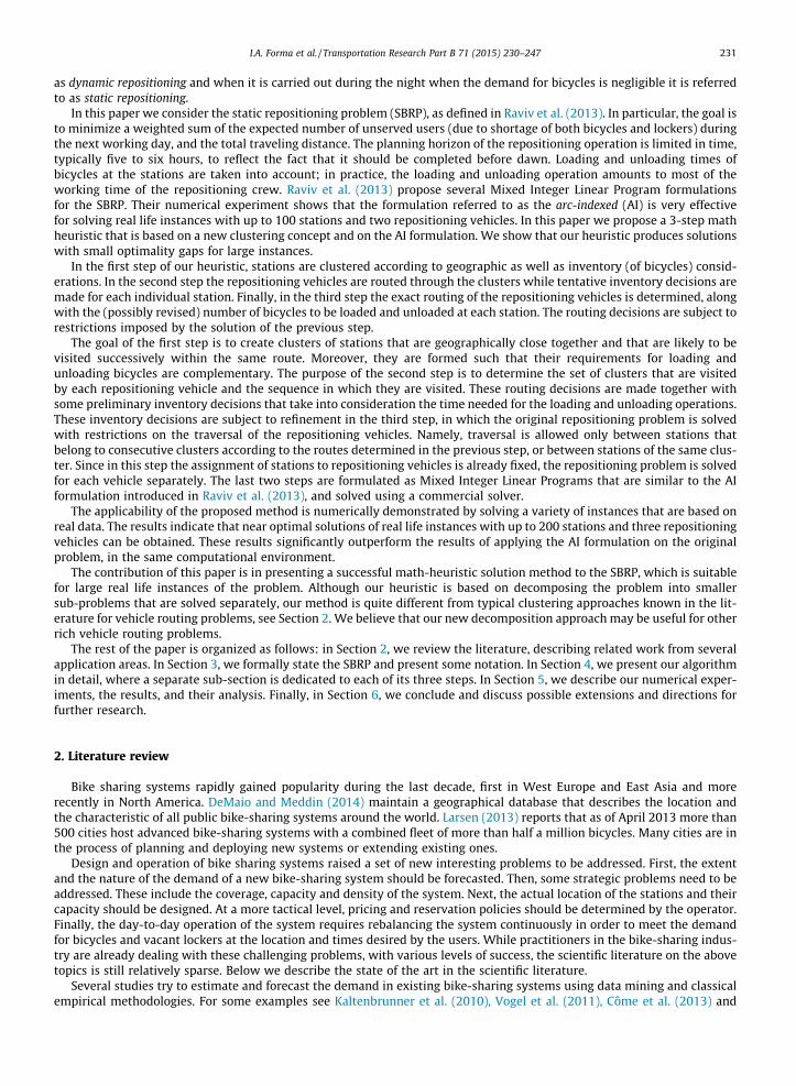
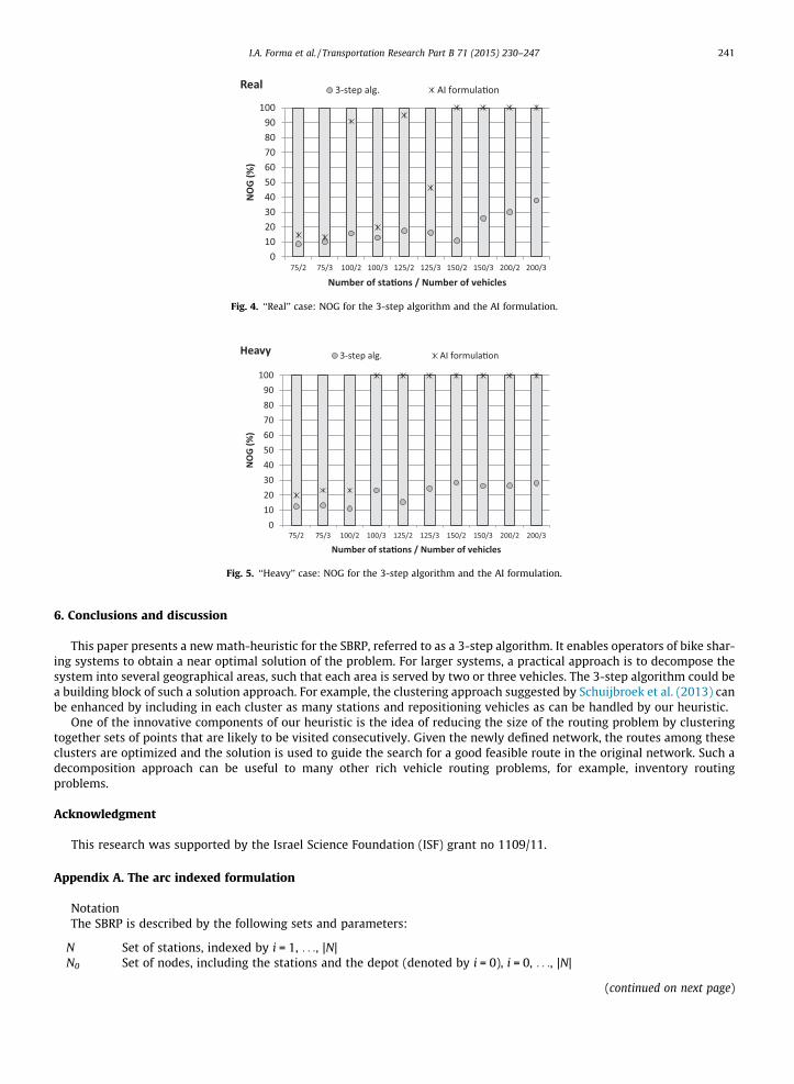
real and heavy workloads. The rightmost three columns present the NOG value (in %) obtained by the AI formulation. In caseswhen a feasible solution could not be obtained within the time limit, no NOG value is reported.

The results presented in Table 3 are visualized in Figs. 3–5 for the light, real and heavy workload, respectively. The verticalaxis represents the normalized optimality gap, in%, where a value of 100% means that no feasible solution was found. Eachbar presents an instance with its number of stations and repositioning vehicles.

We observe that in most cases the 3-step heuristic algorithm outperforms the result obtained from CPLEX using the AIformulation subject to the one hour time limit. There are only two exceptions, out of 30 instances, which refer to theinstances with the smallest number of stations examined, and in which the workload was light. In fact, with the AI formu-lation, for most of the larger instances, we could not even obtain a feasible solution after one hour. The 3-step algorithm, onthe other hand, always delivered feasible solutions that materialized substantial share of the potential improvement. Asexpected, for both methods the NOG is generally lower for smaller instances in terms of the number of stations and vehicles.

We also observe that the NOG obtained by the 3-step algorithm is not very sensitive to the workload. In particular, theNOG values of the heavy workload are always lower than those of the light workload, and in some cases also lower thanthose of the real workload.

The above results show that our 3-step algorithm is a good heuristic for the SBRP with at least 200 stations and threerepositioning vehicles, which represents bike sharing systems of moderate-large size. This is an improvement over previousresults for the same problem, which were able to solve the problem with up to about 100 stations and two repositioningvehicles.

0

10

20

30

40

50

60

70

80

90

100

75/2 75/3 100/2 100/3 125/2 125/3 150/2 150/3 200/2 200/3

NO

G (%

)

Number of sta�ons / Number of vehicles

Light 3-step alg. AI formula�on

Fig. 3. ‘‘Light’’ case: NOG for the 3-step algorithm and the AI formulation.

0 10 20 30 40 50 60 70 80 90

100

75/2 75/3 100/2 100/3 125/2 125/3 150/2 150/3 200/2 200/3

NO

G (%

)


Real 3-step alg. AI formula�on

Fig. 4. ‘‘Real’’ case: NOG for the 3-step algorithm and the AI formulation.

0

10

20

30

40

50

60

70

80

90

100

75/2 75/3 100/2 100/3 125/2 125/3 150/2 150/3 200/2 200/3

NO

G (%

)


Heavy 3-step alg. AI formula�on

Fig. 5. ‘‘Heavy’’ case: NOG for the 3-step algorithm and the AI formulation.


6. Conclusions and discussion

This paper presents a new math-heuristic for the SBRP, referred to as a 3-step algorithm. It enables operators of bike shar-ing systems to obtain a near optimal solution of the problem. For larger systems, a practical approach is to decompose thesystem into several geographical areas, such that each area is served by two or three vehicles. The 3-step algorithm could bea building block of such a solution approach. For example, the clustering approach suggested by Schuijbroek et al. (2013) canbe enhanced by including in each cluster as many stations and repositioning vehicles as can be handled by our heuristic.

One of the innovative components of our heuristic is the idea of reducing the size of the routing problem by clusteringtogether sets of points that are likely to be visited consecutively. Given the newly defined network, the routes among theseclusters are optimized and the solution is used to guide the search for a good feasible route in the original network. Such adecomposition approach can be useful to many other rich vehicle routing problems, for example, inventory routingproblems.

Acknowledgment

This research was supported by the Israel Science Foundation (ISF) grant no 1109/11.

Appendix A. The arc indexed formulation

NotationThe SBRP is described by the following sets and parameters:

N
Set of stations, indexed by i = 1, . . ., |N| N0 Set of nodes, including the stations and the depot (denoted by i = 0), i = 0, . . ., |N|
(continued on next page)


V
Set of vehicles, v = 1, . . ., |V| s0
i
Number of bicycles at node i before the repositioning operation starts ci Number of lockers installed at station i e N0, referred to as the station’s capacity kv Capacity (number of bicycles) of vehicle v e V fi(si) A convex penalty function for station i e N, the function is defined over the integers si = 0, . . ., ci
tij
Traveling time from station i to station j a Weight/scaling factor (in the objective function) of the operating costs relative to the penalty costs T Repositioning time, i.e., time allotted to the repositioning operation L Time required to remove a bicycle from a station and load it onto the vehicle U Time required to unload a bicycle from the vehicle and hook it to a locker in a station
We use the following decision variables:

xijv
Binary variable which equals one if vehicle v travels directly from node i to node j, and zero otherwise yijv Number of bicycles carried on vehicle v when it travels directly from node i to node j. yijv is zero if the vehicle v does
not travel directly from i to j
yL
iv
Number of bicycles loaded onto vehicle v at node i yU
iv
Number of bicycles unloaded from vehicle v at node i qiv Auxiliary variables used for sub-tour elimination constraints si Inventory level at node i at the end of the repositioning operation M An upper bound on the number of arcs in a vehicle’s tour whose length is at most T time units, where the vehicle
visits each station at most once

The Arc Indexed (AI) formulation is the following:

MinXi2N

f iðsiÞ þ aXi2N0

Xj2N0

Xv2V

tijxijv ð11Þ

s.t.

si ¼ s0i �

Xv2V

ðyLiv � yU

ivÞ 8i 2 N0 ð12Þ

yLiv � yU

iv ¼X

j2N0 ;j–i

yijv �X

j2N0 ;j–i

yjiv 8i 2 N0;8v 2 V ð13Þ

yijv 6 kvxijv 8i; j 2 N0; i – j; 8v 2 V ð14Þ

Xj�N0 ;j–i

xijv ¼X

j�N0 ;j–i

xjiv 8i 2 N0;8v 2 V ð15Þ

Xj�N0 ;j–i

xijv 6 1 8i 2 N; 8v 2 V ð16Þ

Xv2V

yLiv 6 s0

i 8i 2 N0 ð17Þ

Xv2V

yUiv 6 ci � s0

i 8i 2 N0 ð18Þ

Xi2N0

ðyLiv � yU

ivÞ ¼ 0 8v 2 V ð19Þ

Xi2N

LyLiv þ UyU

iv

� �þXi2N

ðLy0iv þ Uyi0vÞ þX

i;j2N0 :i–j

tijxijv 6 T 8v 2 V ð20Þ

qjv P qiv þ 1�Mð1� xijvÞ 8i 2 N0; j 2 N; i– j;8v 2 V ð21Þ

xijv 2 f0;1g 8i; j 2 N0 : i– j;8v 2 V ð22Þ


yLiv P 0; yU

iv P 0; integer 8i 2 N0;8v 2 V ð23Þ

yijv P 0 8i; j 2 N0 : i– j;8v 2 V ð24Þ

si P 0 8i 2 N0 ð25Þ

qiv P 0 8i 2 N0;8v 2 V ð26Þ

The objective function (11) minimizes the total cost of the system, consisting of the sum of the penalties incurred at allstations and the total operating costs, appropriately weighted by a factor of a. Note that the objective function consists of asum of convex functions over a discrete set, which can be linearized as described as described below, see (27) and (28).Constraints (12)) are inventory-balance constraints at the nodes (the stations and the depot). Constraints (13) representthe conservation of inventory on the vehicles, and constraints (14) limit the quantity carried on each vehicle to its capacity.These constraints also set the quantity carried on a vehicle to zero when it travels directly from i to j if the vehicle does notuse that arc. Constraints (15) are vehicle flow-conservation equations. Constraints (16) ensure that each station is visited atmost once by each vehicle and constraints (17) (resp., (18)) limit the quantity picked-up by all vehicles from a station (resp.,delivered to a station) to the quantity available there initially (resp., the residual capacity of the station). Note that con-straints (17) also imply non-negativity of the inventory variables, while constraints (18) also ensure that the inventory ateach station and at the depot is bounded by its capacity; therefore, these two restrictions are not written explicitly. Con-straints (19) stipulate that all the bicycles that are loaded onto the vehicles are also unloaded. Constraints (20) limit the totalloading and unloading times plus the travel times to the total time available for the repositioning operation. Constraints (21)are sub-tour elimination constraints that are similar to those of Miller et al. (1960). Finally, (22) and (23) are binary and gen-eral integrality constraints, respectively, and (24)–(26) are non-negativity constraints. Note that the integrality of yijv and si isimplied by the integrality of yL

iv ; yUiv and s0

i .

As mentioned above, we can replace the previous convex terms in the objective function by linear terms:

MinXi2N

gi þ aXi2N0

Xj2N0

Xv2V

tijxijv ð27Þ

and add the following constraints to the formulation:

gi P aiu þ biusi 8i 2 N; u ¼ 0; . . . ; ci � 1 ð28Þ

where gi is the penalty incurred at station i, biu � fi(u + 1) � fi(u), aiu � fi(u) � biu � u"i, "u. We also added the same cut con-straints as detailed into Raviv et al. (2013), in order to speed the solution time.

Appendix B. The arc indexed (AI) formulation adapted to clusters routing (step 2)

We explain how we adapt the notation to the problem definition of this step. We let B = {I1, . . ., In} represent the setof clusters obtained in the first step, B0 = {I0, I1, . . ., In} where I0 = {0} is a cluster which consists of the depot only, and weuse I and J to represent general clusters. In a pre-processing calculation, we set the location of a cluster to be thelocation of the closest station to the center of gravity of the cluster, and denote the travel distance between clustersI and J by tIJ.

In the definitions below, since routing decisions are considered between clusters only, routing decision variables are alsodefined between clusters only. In particular, no routing decision variables are defined between stations. On the other hand,all decision variables that concern the inventory decisions still exist.

The adapted decision variables (relative to the original AI formulation, which is stated in Appendix A):

xIJv
binary variable that equals one if vehicle v travels directly from cluster I to cluster J, and zero otherwise yIJv number of bicycles carried on vehicle v when it travels directly from cluster I to cluster J. yIJv is zero if the vehicle v
does not travel directly from I to J
qIv auxiliary variables, used for sub-tour elimination constraints
The same decision variables (that are the same as in the original AI formulation):

yLiv
number of bicycles loaded onto vehicle v at station i
yUiv
number of bicycles unloaded off of vehicle v at station i
si
inventory level at station i at the end of the repositioning operation (mentioned before)


Arc indexed (AI) formulation adapted to clusters routing

MinXi2N

f iðsiÞ þ aXI2B0

XJ2B0

Xv2V

tIJxIJv ð29Þ

s.t.

si ¼ s0i �

Xv2V

yLiv � yU

iv� �

8i 2 N0 ð12Þ

Xi2I

yLiv � yU

iv� �

¼X

J2B0 ;J–I

yIJv �X

J2B0 ;J–I

yJIv 8I 2 B0;8v 2 V ð30Þ

yIJv 6 kvxIJv 8I; J 2 B0; I – J;8v 2 V ð31Þ

XJ�B0 ;J–I

xIJv ¼X

J�B0 ;J–I

xJIv 8I 2 B0;8v 2 V ð32Þ

XJ�B0 ;J–I

Xv2V

xIJv 6 1 8I 2 B ð33Þ

Xv2V

yLiv 6 s0

i 8i 2 N0 ð17Þ

Xv2V

yUiv 6 ci � s0

i 8i 2 N0 ð18Þ

Xi2N0

yLiv � yU

iv� �

¼ 0 8v 2 V ð19Þ

Xi2N

ðLyLiv þ UyU

ivÞ þXI2B

ðLy0Iv þ UyI0vÞ þX

I;J2B0 :I–J

tIJxIJv 6 T 8v 2 V ð34Þ

qJv P qIv þ 1�Mð1� xIJvÞ 8I 2 B0; J 2 B; I – J;8v 2 V ð35Þ

xIJv 2 f0;1g 8I; J 2 B0 : I – J;8v 2 V ð36Þ

yLiv P 0; yU

iv P 0; integer 8i 2 N0;8v 2 V ð23Þ

yIJv P 0 8I; J 2 B0 : I – J;8v 2 V ð37Þ

si P 0 8i 2 N0 ð25Þ

qIv P 0 8I 2 B0;8v 2 V ð38Þ

In the formulation above, the first term of the objective function (29), which refers to the inventory-related costs, is thesame as in the original AI formulation. (This term is later linearized, similar to (27) and (28) above.) The second term refers tothe operating costs of routing between clusters, rather than between stations as in the original AI formulation. Note that thevalue of the objective function is a lower bound to the real costs of the repositioning problem, since the operating costs donot include the routing between stations within clusters.

As for the constraints, similarly to the definition of the decision variables, those that refer to inventory at the stations havenot changed (Constraints (9), (17)–(19), (23), (25), whose reference number did not change). The constraints that refer to therouting are similar to the original ones, only with a cluster index rather than a station index (Constraints 31, 32, 35, 36, 23,37, 25, 38). Finally, Constraints 30, 33 and 34 have changed slightly. Constraint (30) is a flow conservation constraint, whichapplies now to clusters rather than to stations. In Constraint (33) we assume that each cluster may be visited at most once byall vehicles; this is different from the original formulation in which this constraint is applied to each vehicle separately; thischange is motivated by Step 3 of our algorithm, see Section 4.3. Constraints (34) limit the total loading and unloading timesat stations as well as at the depot, plus the travel times between clusters to the length of time available for the repositioningoperation. In this constraint, routing variables refer again to clusters rather than to stations.

We add the constraints (cuts) that were included in the original formulation of Raviv et al. (2103), adapted to the formu-lation above, i.e., where routing decision variables refer to clusters rather than to stations, and inventory decision variablesare unchanged. We also add the following constraints, which follows from (33):

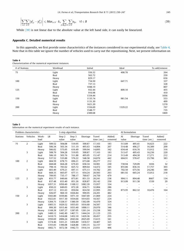
Table 4Charact

# of

75

100

125

150

200

Table 5Informa

Prob

Stati

75

100

125

150

200


Xi2I

Xv2V

yLiv � yU

iv� ��

�� 6 Maxv2V � kvX

J2B0 :J–I

Xv2V

xIJv 8I 2 B ð39Þ

While (39) is not linear due to the absolute value at the left hand side, it can easily be linearized.

Appendix C. Detailed numerical results

In this appendix, we first provide some characteristics of the instances considered in our experimental study, see Table 4.Note that in this table we ignore the number of vehicles used to carry out the repositioning. Next, we present information on

erization of the numerical experiment instances.

Stations Workload Initial Ideal To add/remove

Light 556.32 498.78 264Real 562.72 259Heavy 829.17 656Light 734.50 647.71 337Real 737.13 328Heavy 1048.19 807Light 932.44 809.10 455Real 916.98 410Heavy 1334.44 1056Light 1135.74 981.54 553Real 1131.30 499Heavy 1621.20 1270Light 1556.69 1329.22 797Real 1548.77 735Heavy 2300.68 1869

tion on the numerical experiment results of each instance.

lem characteristics 3-step algorithm AI formulation

ons Vehicles Work-load

LB Step 2value

Step 3value

Shortage Traveltime (sec.)

Added/removed

AIvalue

Shortage Traveltime (sec.)

Added/removed

2 Light 509.52 504.08 519.95 500.87 17,163 183 513.89 495.41 16,623 222Real 506.34 503.34 511.19 495.63 14,004 207 514.48 496.27 16,389 209Heavy 586.02 575.05 616.49 599.94 14,895 342 634.44 616.76 15,912 316

3 Light 508.79 504.28 519.95 500.87 17,163 183 513.47 495.43 16,236 220Real 506.10 503.76 511.88 495.05 15,147 214 513.49 494.30 17,271 212Heavy 537.52 535.88 576.22 548.58 24,876 442 604.91 578.47 23,796 383

2 Light 684.59 678.73 696.21 673.68 20,277 212 – – – –Real 668.68 664.28 679.43 658.34 18,981 230 730.94 729.09 1656 32Heavy 798.16 783.62 825.72 809.64 14,472 345 855.86 836.16 17,757 303

3 Light 683.49 679.21 697.11 675.13 19,782 201 702.50 675.56 24,246 180Real 668.33 665.07 677.11 654.24 20,583 263 681.92 665.24 15,012 218Heavy 709.95 735.17 788.17 760.67 24,750 479 – – – –

2 Light 855.77 849.66 873.81 851.33 20,241 238 904.11 894.48 8667 134Real 837.48 833.40 851.26 828.87 20,142 250 913.09 911.38 1539 29Heavy 1057.31 1050.49 1100.12 1082.39 15,957 334 – – – –

3 Light 850.22 849.03 872.28 836.71 32,004 286 – – – –Real 837.12 831.63 850.04 824.50 22,995 293 873.95 862.32 10,476 164Heavy 926.97 969.10 1026.84 999.95 24,201 482 – – – –

2 Light 1043.80 1039.86 1071.10 1047.69 21,069 224 – – – –Real 1022.81 1017.30 1034.66 1014.03 18,567 224 – – – –Heavy 1284.75 1328.57 1380.39 1362.09 16,470 324 – – – –

3 Light 1005.51 1029.52 1055.03 1016.60 34,587 315 – – – –Real 999.30 1015.46 1033.40 1000.11 29,970 346 – – – –Heavy 1168.28 1207.27 1287.05 1261.24 23,238 502 – – – –

2 Light 1400.12 1442.49 1467.71 1444.24 21,123 235 – – – –Real 1410.73 1434.68 1452.10 1429.36 20,457 255 – – – –Heavy 1950.69 2006.24 2043.04 2025.69 15,615 341 – – – –

3 Light 1374.46 1431.21 1456.80 1418.57 34,407 325 – – – –Real 1355.83 1396.08 1428.88 1393.15 32,157 347 – – – –Heavy 1802.71 1872.58 1942.73 1916.14 23,931 496 – – – –


the results obtained for each instance in this experiment, including the data from which the optimality gaps presented inTables 1–3 in Section 5 were calculated.

The first and second columns in Table 4 denote the number of stations and the workload of each instance. The nextcolumn, entitled ‘‘Initial’’, presents the expected number of shortage events assuming no repositioning is done. This valueis used as an upper bound for the solution value. The column entitled ‘‘Ideal’’ presents the expected number of shortageevents assuming the number of bicycles at each station before the demand commences is optimal (i.e., ideal, ignoring therepositioning effort costs and constraints). The rightmost column in the table specifies the total number of bicycles that needto be added or removed at the stations in order to change the initial state of the system to its ideal state. Note that thisnumber is significantly smaller for the ‘‘Light’’ and ‘‘Real’’ instances compared with the ‘‘Heavy’’ instances. The latter wereartificially created in order to examine the effect of the workload on the performance of the proposed solution method.

Table 5 contains the results of the 3-step algorithm and the AI formulation. The first three columns present the problemcharacteristics of each instance, namely, number of stations, number of vehicles and workload. In the next column we reporton the lower bound of the optimal solution obtained from the MILP solver applied on the original AI formulation, see Appen-dix A. In the next five columns we report on the results of running the 3-step algorithm. First the solution values of Step 2and Step 3 are presented. Note that the former is consistently slightly lower since the model solved in this step does not takeinto account the travel time of the vehicles between the stations of each cluster. In the next two columns the two compo-nents of the objective function are presented: the expected shortage and the travel time. Recall that the value of the solutionis the expected shortage plus a multiplied by the travel time. The number of bicycles that are added and removed at thestations in the solution obtained by the 3-step algorithm is presented next. In the last four columns similar informationis presented with respect to the AI formulation. No information is provided when the problem could not obtain a feasiblesolution within the time limit of one hour.

References

Baldacci, R., Bartolini, E., Laporte, G., 2010. Some applications of the generalized vehicle routing problem. J. Oper. Res. Soc. 61 (7), 1072–1077.Battarra, M., Erdogan, G., Vigo, D., 2014. Exact algorithms for the clustered vehicle routing problem. Oper. Res. 62 (1), 58–71.Berbeglia, G., Cordeau, J.-F., Gribkovskaia, I., Laporte, G., 2007. Static pickup and delivery problems: a classification scheme and survey. TOP 15 (1), 1–31.Chemla, D., Meunier, F., Wolfler-Calvo, R., 2013a. Bike sharing systems: solving the static rebalancing problem. Dis. Optim. 10 (2), 120–146.Chemla, D., Meunier, F., Pradeau, T., Wolfler-Calvo, R., Yahiaoui, H., 2013b. Self-service bike sharing systems: simulation, repositioning, pricing. Working

paper.Chow, J.Y.J., Sayarshad, H.R., 2014. Symbiotic network design strategies in the presence of coexisting transportation networks. Transp. Res. Part B 62 (1), 13–

34.Clarke, G., Wright, J.W., 1964. Scheduling of vehicles from a central depot to a number of delivery points. Oper. Res. 12 (4), 568–581.Côme, E., Randriamanamihaga, A., Oukhellou, L., Aknin, P., 2013. Spatio-temporal analysis of dynamic origin-destination data using latent

dirichlet allocation. Application to the Vélib’ Bike Sharing System of Paris. Working paper.Contardo, C., Morency, C., Rousseau, L.-M., 2012. Balancing a dynamic public bike-sharing system. Working paper.DeMaio, P. and Meddin, R., 2014. The bike sharing blog, <http://bike-sharing.blogspot.com/>, observed at April 11, 2014.Erdogan, G., Laporte, G., Calvo, R.W., 2013. The one-commodity pickup and delivery traveling salesman problem with demand intervals. Working paper.Fisher, M.L., Jaikumar, R., 1981. A generalized assignment heuristic for vehicle routing. Networks 11 (2), 109–124.Forma I., Raviv T., Tzur M., 2010. The static repositioning problem in a bike-sharing system. In: Proceeding of the 7th triennial symposium on transportation

analysis (TRISTAN), 279–282.Fricker, C., Gast, N., 2015. Incentives and regulations in bike-sharing systems with stations of finite capacity. Eur. J. Transp. Logist. (forthcoming).Gillett, B.E., Miller, L.R., 1974. A heuristic algorithm for the vehicle dispatch problem. Oper. Res. 22 (2), 340–349.Hernández-Pérez, H., Salazar-González, J.-J., 2004. A branch-and-cut algorithm for a traveling salesman problem with pickup and delivery. Dis. Appl. Math.

145 (1), 126–139.Kaltenbrunner, A., Meza, R., Grivolla, J., Codina, J., Banchs, R., 2010. Urban cycles and mobility patterns: exploring and predicting trends in a bicycle-based

public transport system. Perv. Mobile Comput. 6 (4), 455–466.Kaspi, M., Raviv, T., Tzur, M., 2014a. Parking reservation policies in one-way vehicle sharing systems. Transp. Res. Part B 62 (1), 35–50.Kaspi, M., Raviv, T., Tzur, M., Galili, H., 2014b. Analysis and performance bounds of parking reservation policies in vehicle sharing systems. Working paper.Kloimüllner, C., Papazek, P., Hu, B., Raidl, G.R., 2014. Balancing bicycle sharing systems: an approach for the dynamic case. In: Blum, C., Ochoa, G. (Eds.),

EvoCOP 2014, Lecture Notes in Computer Science 8600, pp. 73–84.Laporte, G., Semet, F., 2002. Classical heuristics for the capacitated VRP. In: Toth, P., Vigo, D. (Eds.), The Vehicle Routing Problem. SIAM, pp. 109–128.Larsen, J., 2013. Plan B updates – bike-sharing programs hit the streets in over 500 cities worldwide, <http://www.earth-policy.org/plan_b_updates/2013/

update112>, published April 25, 2013, observed on April 11, 2014.Lin, J.-R., Yang, T.-H., 2011. Strategic design of public bicycle sharing systems with service level constraints. Transp. Res. Part E 47 (2), 284–294.Miller, C.E., Tucker, A.W., Zemlin, R.A., 1960. Integer programming formulations and traveling salesman problems. J. ACM 7 (4), 326–329.Nair, R., Miller-Hooks, E., Hampshire, R.C., Bušic, A., 2013. Large-scale vehicle sharing systems: analysis of vélib’. Int. J. Sust. Transp. 7 (1), 85–106.Pessach, D., Raviv, T., Tzur, M., 2014. Dynamic repositioning in a bike sharing system. Working Paper.Pfrommer, J., Warrington, J., Schildbach, G., Morari, M., 2014. Dynamic vehicle redistribution and online price incentives in shared mobility systems. IEEE

Trans. Intell. Transp. Syst. 15 (4), 1564–1578.Raidl, G.R., Hu, B., Rainer-Harbach, M., Papazek, P., 2013. Balancing bicycle sharing systems: improving a VNS by efficiently determining optimal loading

operations. Hybrid Metaheuristics, Lecture Notes in Computer Science, vol. 7919. Springer-Verlag, Berlin Heidelberg, pp. 130–143.Rainer-Harbach, M., Papazek, P., Hu, B., Raidl, G.R., 2013. Balancing bicycle sharing systems: a variable neighborhood search approach. Evolutionary

Computation in Combinatorial Optimization, Lecture Notes in Computer Science, vol. 7832. Springer-Verlag, Berlin Heidelberg, pp. 121–132.Raviv, T., Tzur, M., Forma, I., 2013. Static repositioning in a bike-sharing system: models and solution approaches. Eur. J. Transp. Logist. 2, 187–229.Raviv, T., Kolka, O., 2013. Optimal inventory management of a bike-sharing station. IIE Trans. 45 (10), 1077–1093.Romero, J.P., Ibeas, A., Moura, J.L., Benavente, J., Alonso, B., 2012. A simulation-optimization approach to design efficient systems of bike-sharing. Proc. Soc.

Behav. Sci. 54 (4), 646–655.Rudloff, C., Lackner, B., 2014. Modeling demand for bicycle sharing systems – neighboring stations as a source for demand and a reason for structural breaks.

In: the proceeding of the Transportation Research Board 93rd Annual Meeting.Schuijbroek, J., Hampshire, R., van Hoeve, W.-J., 2013. Inventory rebalancing and vehicle routing in bike sharing systems. Working paper.

http://refhub.elsevier.com/S0191-2615(14)00172-6/h0005







http://bike-sharing.blogspot.com/









http://www.earth-policy.org/plan_b_updates/2013/update112

http://www.earth-policy.org/plan_b_updates/2013/update112















Shu, J., Chou, M., Liu, Q., Teo, C.-P., Wang, I.-L., 2013. Models for effective deployment and redistribution of bicycles within public bicycle-sharing systems.Oper. Res. 61 (6), 1346–1359.

Shu, J., Teo, C.-P., Shen, Z.J.M., 2005. Stochastic transportation-inventory network design problem. Oper. Res. 53 (1), 48–60.Vogel, P., Greiser, T., Mattfeld, D.K., 2011. Understanding bike-sharing systems using data mining: exploring activity patterns. Proc. Soc. Behav. Sci. 20,

514–523.Waserhole, A., Jost, V., 2015. Pricing in vehicle sharing systems: optimization in queuing networks with product forms, Eur. J. Transp. Logist. (forthcoming).






A 3-Step Math Heuristic for the Static Repositioning Problem in Bike-Sharing Systems

Documents

Transcript of A 3-Step Math Heuristic for the Static Repositioning Problem in Bike-Sharing Systems