9337-9181.pdf - CEJSH

• F I N A N S E I P R A W O F I N A N S O W E •

www.finanseiprawofinansowe.uni.lodz.pl 149

• Journal of Finance and Financial Law •

Grudzień/December 2020 ● vol. 4(28): 149–174

THE EFFECTIVENESS OF THE TRANSACTION SYSTEMS

ON THE DAX INDEX

M.Sc. in Economics Marek Trembiński Warsaw School of Economics, Finance and Accounting, Securities Broker

Assistant Professor, Ph.D. Joanna Stawska

Faculty of Economics and Sociology, University of Lodz

ORCID: https://orcid.org/0000-0001-6863-1210

Abstract

The purpose of the article/hypothesis: The aim of this article is to examine the effectiveness of trading systems built on the basis of technical analysis tools in 2015–2020 on the DAX stock exchange index. Efficiency is understood as generating positive rates of return, taking into account the risk incurred by the investor, as well as achieving better results than passive strategies. Presenting empirical evidence implying the value of technical analysis is a difficult task not only because of a huge number of instruments used on a daily basis, but also due to their almost unlimited possibility to modify parameters and often subjective evaluation.

Methodology: The effectiveness of technical analysis tools was tested using selected investment strategies based on oscillators and indicators following the trend. All transactions were carried out on the Meta Trader 4 platform. The analyzed strategies were comprehensively assessed using the portfolio management quality measures, such as the Sharpe measure or the MAR ratio (Managed Account Ratio).

Results of the research: The test results confirmed that the application of described investment strategies contributes to the achievement of effective results and, above all, protects the portfolio against a significant loss in the period of strong turmoil on the stock exchange. During the research period, only two strategies (Ichimoku and ETF- Exchange traded fund) would produce negative returns at the worst possible end of the investment. At the best moment, however, the „passive” investment achieved the lowest result. Looking at the final balance at the end of 2019, as many as four systems based on technical analysis were more effective than the „buy and hold” strategy, and at the end of the first quarter of 2020 – all of them. When analyzing the management quality measures, it turned out that taking into account the 21 quarters, the passive strategy had the lowest MAR index. The Sharpe’s measure is also relatively weak compared to the four leading strategies.

Keywords: technical analysis, trading systems, DAX index, stock exchange, investment strategies.

JEL Class: G11, G14, G15, O24.

http://dx.doi.org/10.18778/2391-6478.4.28.09

© by the author, licensee Łódź University – Łódź University Press, Łódź, Poland. This article is an open access articledistributed under the terms and conditions of the Creative Commons Attribution license CC-BY-NC-ND 4.0

150

www.finanseiprawofinansowe.uni.lodz.pl

Marek Trembiński, Joanna Stawska

INTRODUCTION

Technical analysis is one of the oldest areas of market science although many

investors and academics see it as a useless tool in making investment decisions,

and even as „reading tea leaves” or a self-fulfilling forecast. Meanwhile, one of

the fundamental aspects of technical analysis is the study of market behavior by

using charts to predict future price levels in the light of rapidly changing human

perception, which determines quick actions that would not be possible using only

the fundamental analysis. In order to fully appreciate the technical analysis, it is

first of all necessary to understand its assumptions, which are based on three

rational pillars. The first one tells us that the market discounts everything. This

means that all political, fundamental or psychological factors affecting the market

price of a commodity are fully reflected in the price of that commodity, and

therefore, studying price behavior is a self-sustaining approach. Perhaps this

approach seems to be an oversimplification, but after much reflection it is hard to

disagree with it. The second premise is that prices are trending. Studying the charts

comes down to identifying trends at an early stage, enabling us to trade in line

with their direction. Moreover, trends tend to continue running in the current

direction, rather than change, until there are significant signs of a possible

reversal. The third pillar is based on patterns proven in the past and is based on

the study of the human psyche, which remains unchanged. This means that history

likes to repeat itself, so an important factor in understanding the future is the

proper analysis of historical quotations [Murphy 1995: 2–4]. Technical analysis

has many strengths, but limitations as well. A big plus is the fact that it is based

on historical data such as prices, volume or a number of open positions. This

information is publicly available, which allows market participants to relatively

easily translate it into a chart and analyze it. Thanks to the above data, it is possible

to determine not only the liquidity of a given stock, but also to set support and

resistance levels as well as trend lines. Moreover, technical analysis is a universal

method, regardless of whether we study the market of raw materials, shares,

currencies or precious metals. Another advantage is the application for any

investment horizon although it is the most popular among short-term players.

Contrary to the fundamental analysis, specialist knowledge on the interpretation

of financial statements is also not required, which, when using creative accounting

or placing given assets or liabilities in a different category, may have a negative

impact on the company’s reliable valuation.

Critics of technical analysis point out the lack of correlation between

historical and future prices. As a result, the tools used in the past do not have to

prove useful in the future, leading investors to lose trades [Pająk 2013: 132–134].

In some situations, we also receive contradictory information that is mutually

exclusive – namely, one indicator gives a sell signal and the other gives a buy



The Effectiveness of the Transaction Systems…

signal, which makes it difficult to take a position on the right side of the market.

Among the disadvantages (or perhaps advantages?) of the analysis, there is also

a significant element of subjectivism, while the fundamental assessment of values

is related to the interpretation of economic and financial data. Meanwhile, the

subjective approach leads to a heuristic error, called the „backward thinking

effect”. For this reason, the layouts on the chart play out completely differently in

retrospect than at the time of trading [www5, accessed 2.02.2020]. The article

consists of the following parts: introduction, the theoretical part in which the

researched investment strategies are described, and then the empirical part in

which the effectiveness of a total of six transaction systems built on the basis of

technical analysis was checked, using two selected measures of portfolio

management quality, i.e. the Sharpe indicator and MAR, and then additionally

compared the previously tested six trading systems with the passive „buy and

hold” strategy also using the Sharpe and MAR ratios. The article ends with

conclusions of the conducted study.

1. CONSTRUCTION OF TRANSACTION SYSTEMS

Many novice investors are looking for a magic indicator that will allow them to

multiply their capital. When it starts to work, they feel as if they have discovered

the Holy Grail and the path to success seems simple. The reality can be quite

different, however, as markets are too complex to be analyzed using only one

measure. Hence, this article will examine six trading systems created on the basis

of technical analysis, such as: 1) the strategy of moving averages and ADX

indicator; 2) MACD and Parabolic SAR strategy; 3) the strategy based on RSI and

Bollinger bands; 4) Ichimoku Kinko Hyo Technique; 5) the strategy using

Commodity Channel Index and Donchian Channel; 6) the strategy based on the

stochastic oscillator and the Keltner Channel, and then comparing them with the

passive strategy, i.e. „buy and hold”. Before these strategies were compared by

using the Sharpe index and MAR, the structure of the analyzed strategies is

presented below.

1.1. Moving averages strategy and ADX indicator

Each investment strategy requires not only setting a convenient entry point, but

also an exit from the position in order to properly manage risk. Moving averages

are used to detect long-term trends as well as day trading. They smooth out market

vibrations and short-term volatility of quotations, which allows us to identify

where the market is heading. On the other hand, they do not work for


152



consolidation, generating many wrong signals. They also do not measure the

strength of the current trend [LeBeau and Lucas 1998: 90–92].

One of the simplest and one of the most effective systems is the one moving

average system. The buy signal occurs when the rate crosses the average line from

the bottom, and the sell signal occurs when the rate crosses the average line from

the top. It is a simple system that implies a continuous presence on the market, but

it is worth using additional filters [LeBeau and Lucas 1998: 96–97; Borowski

2019]. However, the system based on two averages is used more often. Various

combinations of N values are possible, e.g. 3- and 12-period mean or the popular

Richard Donchian system based on 5 and 20 periods. The principle of using

averages is simple: we buy when the shorter average (faster) crosses the slower

average from the bottom. We do the opposite while opening a short position.

In order to build a better and more comprehensive system, it is worth adding

the Directional Movement Index (DMI) to the moving averages. The structure of

the system was proposed by J. Welles Wilder in the 1970s. The method not only

identifies the current trend, but also provides information whether it is fast enough

to be worth following. The DMI indicator consists of three lines [www16,

accessed 27.02.2020]:

– ADX (Average Directional Movement Index),

– DI+ (Directional Indicator +),

– DI– (Directional Indicator –).

Directional movement is the range of price fluctuations in a given period that

is outside the extremes of the previous period. For example, if today’s price range

is above yesterday’s, then the directional movement is positive (+DM), if below

negative (–DM). If today’s trading range is within yesterday’s range or is

symmetrically above and below it, then DM = 0 (no movement). After

determining the directional movement, it is necessary to calculate – swing range

– the so-called true range. TR is the largest of the three values::

– the difference between today’s – maximum and minimum or

– today’s maximum – and yesterday’s closing price

– today’s minimum and yesterday’s closing price.

To calculate the daily directional indicators (+DI) and (–DI), divide (+/–) the

DM by the TR, thanks to which the directional traffic is presented as a percentage

value in relation to the range of fluctuations on a given day. Subsequently, the

lines should be smoothed using e.g. a 13-day moving average. When +DI13 is

above –DI13 we are dealing with an uptrend, if it is below – with a downtrend.

Buy or sell signals are generated when the lines cross. At the end, the ADX

(smoothed DX) indicator is calculated, which goes up when prices are moving in

one specific direction [Elder 2018: 136–138]. The DX directional index is

determined by the following formula:




DX = (+DI13 − −DI13)x100+DI13 + −DI13

In the literature, the value of the ADX indicator below 20 points is considered

a weak trend, therefore, other indicators should be used. As the ADX level rises,

traders should be driven by trend following systems (e.g. moving average).

A reading above 45 points indicates a very strong trend and increases the

probability of a correction [Borowski 2018: 127].

The ADX can be used as a filter with a strategy based on two moving averages

or the crossing of the +DI and –DI lines, which can also be used to play against

the trend. A sell signal appears when the +DI line reaches extremely high values

(e.g. 40 points) and the –DI line shows extremely low values (below 10 points)

[www12, accessed 27.03.2020]. The disadvantage of the ADX indicator is that it

only starts to increase after the + DI and –DI lines intersect.

1.2. MACD and Parabolic SAR Strategies

Indicators, commonly called oscillators, allow you to pinpoint the stage of a trend

and pinpoint the moment when the trend loses its momentum. They have been

applied in technical analysis because they express the pace at which market prices

change. Strong momentum suggests a healthy trend, a weak one warns that the

price movement may end. Extreme momentum values can accompany short-term

depletion moments, showing overbought or oversold conditions, which increases

the likelihood of a correction.

The MACD indicator is primarily popular with traders because of its great

flexibility as a tool to play with and against the trend. It was constructed by Gerald

Apple and presents the difference of two exponential moving averages (12 and 26

EMA) together with a 9-period mean of this difference, which is the signal line.

The result is a smooth oscillator with a wide range of applications. Trade opening

signals are generated by breakout of the zero line, crosses of the signal line,

oversold and overbought situations as well as divergences. The convergence and

divergence of the moving averages reflect the approaching or receding of the

averages depending on the speed and changes in the direction of the rates [Etzkorn

1999: 33].

The sell signal is generated when the MACD fast line crosses the signal line

from above, both of them being positive. The signal is all the more important the

higher the intersection above the zero line occurs. Thus, breakthroughs below line

0 should be ignored. A buy signal will appear in the opposite way. Similarly, the

lower the intersection below the 0 line, the more reliable it is. It should also be

remembered that, unlike other oscillators such as the RSI or the stochastic


154



oscillator, the Moving ACD has no lower or upper fluctuation limits [Bar 2001:

108–109].

The MACD is an indicator of an auxiliary nature and its application should

be subordinated to the basic trend analysis. It can generate a lot of false signals in

the initial phase of a trend, so it is better suited at the end of mature trends. Such

information can be provided by a positive or negative divergence. For example,

a negative divergence occurs when the MACD lines are well above the 0 level and

begin to decline while prices continue to hit new maximus. This is often a warning

that a price peak is forming [Murphy 2017: 232].

The strategy may be complemented by the Parabolic Stop and Reversal

indicator developed by Wells Wilder, which performs very well in clear vertical

trends. The PSAR is obviously an indicator of the prevailing trend direction, but

it also proves to be useful in targeting levels of defense orders. It is rarely used as

a single tool, but usually in building simple trading systems in conjunction with

oscillators [www7, accessed 30.03.2020]. The very name of the indicator comes

from the arrangement of dots placed above and below the prices of the instrument,

the shape of which resembles a parabola. To calculate the value of the indicator,

the following recursive formula is adopted [www2, accessed 28.02.2020]:

PSARt = PSARt–1 + AFt–1 x (EPt–1 – PSARt–1),

where:

PSARt – the value of the Parabolic parameter at time t,

AF – the acceleration factor that increases when a new high is reached for long

positions or a new low is for short positions. Wilder’s proposed value is 0.02,

increasing in 0.02 steps until it reaches 0.18–0.21,

EF – lowest or highest price recorded in the current trend.

It should be remembered that in a sideways trend the indicator is practically

useless. Then it provides delayed signals, which, due to the low volatility of price

movements, makes it difficult to conduct profitable transactions [Borowski 2017:

114].

In the above strategy, the condition for opening a long position is that the

MACD indicates an uptrend and the position of the parabolic dot under the price.

Conversely, in case of opening a short position the parabolic should be above the

price and the MACD oscillator should indicate a downward movement. In

addition, traders often use the PSAR as their stop loss level, which is set at the last

dot. When the trend accelerates, the dots begin to move away from each other,

which allows us to hedge unrealized gains.




1.3. Strategy based on RSI and Bollinger Bands

Another strategy commonly used in the financial markets consists of the Relative

Strength Index (RSI) oscillator and Bollinger bands. This is one of the contrarian

strategies because it involves opening positions against the current trend despite

the famous saying among traders – „the trend is your friend”.

The RSI belongs to the group of momentum indicators which inform

investors about the strength and maturity of the current market trend. It was

developed by the aforementioned J.W. Wilder in the 1970s. The indicator

illustrates the relationship between upward and downward movements in closing

prices in a given period, and then normalizes the results so that the index values

vary between 0 and 100. The methodology for calculating the RSI value is defined

by the following formula [Nowakowski 2003: 58]:

RSI= 100 – 1001+(Ui,nDi,n),

where: Ui,nDi,n = (average of positive price changes in n sessions) / (average of negative

price changes in n sessions).

A quotient of sums can also be used instead of quotient of means. Wilder

himself proposed exponential means although analysts use other averages as well.

Most often, 9, 14 or 21 periods are taken as n, and the longer the period, the fewer

signals the oscillator generates. When making investment decisions while taking

into account the RSI, investors pay attention to emerging divergences and levels

of oversold and overbought. Divergence occurs when the RSI starts to decline

despite further price increases and the next peak of the indicator is below the

previous one. Usually, the overbought level is defined when the index exceeds 70,

but during a bull market, the value of 80 can also be adopted. The oversold zone

is bounded by the level of 30 or 20 points [Czekała 1997: 57]. When an indicator enters an overbought or oversold zone, it is a warning

signal of a possible trend reversal, but relying solely on the relative strength index

can lead to huge losses. This is because in a bullish or bearish period, the RSI is

often in the overbought or oversold zone for a long time, so it is important to use

it in conjunction with another technical analysis tool [Czekała 1997: 59]. The oscillator gives quite good signals when a given value is in a horizontal trend. In

this case, a buy signal is generated when the indicator rises above the oversold

level, and a sell signal is generated when the index drops below the overbought

level.


156



Unlike most indicators, Bollinger Bands is not a static indicator and changes

its shape based on recent prices and accurate measurement of momentum and

volatility. The very mechanism of this tool is relatively simple. The middle line is

a moving average, usually calculated for the closing prices of subsequent sessions.

The other two lines are separated by a certain number of standard deviations of

quotations for the adopted period. Typically a 20-period moving average and two

standard deviations are used. These are not randomly established parameters as

they have strong statistical foundations. The three-sigma law tells us that 68.2%

of the observations are within +/– 1 deviation from the mean, while among the

2 deviations the probability increases up to 95.4%. In the range of 3 deviations, it

is 99.7% of observations [www1, accessed 3.03.2020].

In periods when the market is in a sideways trend, it should move between

extreme bands. Reaching the bottom line is then treated as a buy signal,

conversely, a sell signal appears near the upper band. As the volatility increases,

the bands will deviate more and more from the moving average. Additionally,

while setting the standard deviation, multiplicity parameter at the level of 2.5

results in the fact that the price reaches the lower or upper band less often, which

makes the meaning of such a signal more reliable [Kochan 2009: 208 209].

A lot of information from Bollinger Bands can be used to analyze the strength

of a trend. During strong trends, the price stays close to the low or high line, and

a pullback when the trend continues indicates a weakening momentum. On the

other hand, repeated attempts to get the course close to the outer rim, which fail –

signal a lack of strength [www8, accessed 2.04.2020].

The strategy based on the Bollinger bands and the RSI oscillator generates

a sell signal when the price reaches the upper band and is rejected there, while the

relative strength index is in the overbought zone. The occurrence of divergence

may also be an additional confirmation. A buy signal is generated inversely. We

buy when the price bounces from the bottom line and the RSI oscillator shows

a value below 30. The unquestionable advantage of the strategy is the combination

of the leading indicator (RSI) with the lagging indicator (BB). The disadvantages

include the fact that if you rely on a contrarian strategy, without the proper setting

of defense orders, you can suffer severe losses. Corrective movements are

shallower than directional movements, which limits their potential.

1.4. Ichimoku Kinko Hyov Technique

This strategy that literally translates to „one glance equilibrium chart” was

developed in 1968 by Goichi Hosoda. Ichimoku and consists of 5 lines [Bąk 2015: 36]:




– conversion line – tenkan sen,

– base line – kijun sen,

– lagging line – chikou span,

– leading span A - senkou span A,

– leading span B – senkou span B.

The conversion line is the average of the high and low over the last 9 periods

(e.g. the last 9 day candles). Usually, it is closest to the current price and sets the

first support or resistance level when a correction occurs.

Kijun sen is calculated in the same way as tenkan sen, but takes into account

the last 26 periods. After the return line, it is another, but definitely stronger,

resistance or support.

The chikou span is a line that represents the current closing price but shifted

back 26 periods. The principle is as follows: when it is above the price, it is an

uptrend, if below the price – it defines a downward trend. The delayed line does

not generate trading signals, but is a perfect complement to other indicators

[www14, accessed 15.03.2020].

The first of the lines forming the so-called Ichimoku (Kumo) cloud is senkou

span A. It is calculated by adding tenkan and kijun values together, then dividing

the sum by 2 and shifting it forward 26 periods, whereby it is classified as a leading

indicator. In other words, it provides information about the future potential

behavior of the course. The second line, senkou span B, is the result of calculating

the average of the maximum and minimum 52 candles and also shifting by

26 periods forward. The area between them is called the cloud, and depending on

which senkou line is higher, it is called an upward or downward cloud. Span B

often remains flat. Kumo provides the investor with a lot of information. The cloud

can be rising (Span A above Span B) and falling (Span A below Span B). The

thickness of the cloud is also important. The thicker it is, the less likely it gets that

the rate will break its level and the current trend will be reversed. Moreover, it

works very well as support and resistance levels [Elliott 2007: 36–40].

A strategy based on the first two lines can generate three signals: strong,

neutral and weak. A strong buy signal is generated when tenkan sen pierces from

below the Kijun sen above the cloud. A similarly strong sell signal occurs when

tenkan sen crosses the top of the kijun sen below the kumo. Neutral is observed

when the lines intersect within the cloud. It shows that investors are indecisive

and the rate may exit from consolidation both upwards and downwards. A weak

buy signal occurs when the cross occurs below the cloud, which is treated as

a strong price resistance. The interpretation of the line arrangement is the same as

in the case of the strategy based on two moving averages. Another impulse for

stock exchange players is the price going out of the cloud. Long positions should

be opened when the candle closes above the cloud. Conversely, we open short


158



positions – when the candle’s closing is below the kumo. The third buy signal is

the behavior of the chikou span line with respect to price. If the lagging line

crosses the price or goes above it, it confirms the current uptrend in the market.

Therefore, we do not buy when the chikou span is below the rate. Similarly, we

do not open positions when candles are drawn in the cloud range, as this proves

that the consolidation prevails on the market [Oziemczuk 2011: 61–63].

Therefore, the strongest buy signal is to take a long position when three

conditions are simultaneously met: 1) Tenkan sen crosses kijun sen from the

bottom above kumo; 2) the rate will go above the cloud (the higher the more

reliable the break); 3) Chikou span is above the price.

The Ichimoku technique is applicable in all financial markets: stocks, bonds,

commodities, currencies or indices [Borowski 2001: 3].

1.5. Strategy using the Commodity Channel Index and the Donchian Channel

The CCI oscillator was created by Donald Lambert and first described in 1980.

Initially, it gained the popularity mainly on commodity markets, but over time it

began to be used also in other markets. The indicator is used to trade with the

trend, but because it acts like an oscillator, it can also be used to identify turning

points [Frierdich 2013: 256].

CCI is based on a mathematical formula, the result of which is a value that

expresses the statistical distance between the price of a given asset and a moving

average. When the distance is relatively large, we assume that a trend has formed,

and we open a position in its direction. The formula for calculating the CCI value

is as follows [www3, accessed 24.04.2020]:

CCI = (typical price – moving average) / (0,015 x mean deviation)

According to the author’s concept, a typical price is nothing more than the

arithmetic mean of the following three values: highest, lowest and closing. As for

the moving average, it was originally calculated on the basis of 20 periods, but is

now more and more often based on 14 periods. In the denominator, Donald

Lambert took the constant value of 0.015 so that most of the observations fell in

the range of –100 to +100. The CCI can therefore be positive or negative. The

author of the indicator signaled the opening of long positions when the oscillator

exceeded +100 points and their closing when it fell below this round limit. On the

other hand, short positions should be concluded after exceeding the level of –100

points and closed when returning to the –100 line. This approach, however, has

quite a significant disadvantage, namely overlooking the entire initial phase of the

emerging trend. Therefore, in the literature, we can meet with recommendations




to open long position after breaking the 0 level from the bottom and the short

position after crossing from the top [www13, accessed 15.04.2020].

The formula of the Donchian Channel is relatively simple. The upper band is

the maximum, and the lower band is the minimum of the last n periods. The

presumed value of the n parameter on most trading platforms is 20, but it can be

modified depending on the investment horizon and the financial instrument. As

a rule, a buy signal is generated when the rate is above the current level of the

upper band. Short positions should be opened when the price is below the most

recent reading of the lower band of the channel. Therefore, the Donchian-based

trading system assumes that positions should be concluded when a significant

support or resistance breaks. If we want to trade on the basis of the arithmetic

mean of external bands, the trading signals are analogous to the moving average

[www17, accessed 28.03.2020].

An exemplary trading system based on the CCI and Donchian Channel may

generate a buy signal when the rate breaks the upper limit of the channel and the

CCI exceeds the 100 points limit. To capture most of the traffic, it is enough for

the CCI to show a positive value, but this reduces the reliability of the indicator.

1.6. Strategy based on the stochastic oscillator and the Keltner Channel

In spite of the fact that the very word „stochastic” refers to the randomness that

every investor tries to avoid in analyzing financial markets, the stochastic

oscillator is one of the most widely used tools. It was developed by George Lane

in the late 1950s. The stochastic oscillator concept assumes that during a strong

upward trend, closing prices will run around the highs recorded during a given

session, while in a downtrend – near lows. Similar to the RSI, the tool identifies

overbought and oversold levels, indicating the exhaustion or potential of the

current trend. The indicator is constructed using two lines – %K and %D. The first

of them is the so-called the „fast oscillator”, the second – is known as „slow

oscillator”. The %K line measures the strength of a price movement compared to

the price range over a given period. To calculate the value of the fast %K

oscillator, you need to calculate the difference between the last closing price and

the minimum price from e.g. the last 5 sessions. We divide the obtained result by

the difference between the highest and the lowest value recorded during the tested

interval (in this case 5 sessions). In order to get a value from 0 to 100, the quotient

is multiplied by 100. The levels of overbought and oversold are defined in the

same way as for the RSI oscillator, so we need the second %D line to refine the

indicator. There is a 3-period simple moving average of the %K line and is most

often shown as a dotted line on trading platforms. Using both lines we get a more

reliable indicator that generates buy and sell signals every time the %K line


160



crosses the %D line. The best signals are in the oversold or overbought zone.

A long position should be open when, in the oversold zone, the %K line crosses

the %D line from the bottom. A short position, on the other hand, when the %K

line crosses the %D line from the top at overbought levels. Analyzing the course

of a stochastic oscillator can also provide other valuable information, such as

a bullish or bearish divergence. We encounter the former when prices set lower

and lower lows, while the stochastic begins to rise. If the stochastic oscillator goes

down when prices start to rise, it is a bearish divergence. In both situations,

a warning appears about a possible reversal of the current trend [Rockefeller 2012:

267–270].

The author of the second indicator is Chester Keltner, known as a commodity

trader. While the Keltner Channel may resemble the more well-known Bollinger

Bands in the technical analysis theory, in reality its use and design differ from the

Bollinger Bands described above. The main difference is that the outer bands do

not rely on standard deviation but use a different measure of volatility, which is

ATR – Average True Range, developed by J. Wilder. So the price swing range is

just a number, so we need to average the TR over several days to get the ATR.

The increase in this indicator tells us about the greater volatility in the market. For

his calculations the author of the tool used the 14-session moving average

[Jabłoński 2006: 32]. Returning to the design of the Keltner Channel, however, the middle line is

the 20-day exponential moving average. To plot the lower and upper band, we

subtract and add the ATR value multiplied by the coefficient, which, according to

the literature, should be 2 although it can be modified for a given instrument. The

greater the value of the coefficient, the wider the channel and vice versa. Investors

use the Keltner Channel in two ways. The first one involves playing „from band

to band” and works best during consolidation. The second way is to open

a position after breaking the outer band, which confirms the strength of the current

trend. When the price closes over the high band, a buy signal is generated. When

the price closes below the lower band, we open short positions [www15, accessed

20.03.2020]. However, the breakout strategy should be supplemented with e.g.

ADX.

The above strategy based on the stochastic oscillator and the Keltner Channel

may suggest opening a long position when in the oversold zone the %K line breaks

the %D line from the bottom and the price broke below the bottom band of the

channel and starts to come back to it. Short – when the %K line crosses the top of

%D in the overbought zone and the price is above the upper band of the channel.

The trading systems described above are examples of technical analysis

indicators that can be freely modified not only in terms of the size of the

parameters, but also their skillful replacement.




2. TESTING OF TRADING SYSTEMS ON THE DAX STOCK INDEX

DAX (Deutscher Aktienindex) is the main German stock index, which includes

30 largest companies whose total capitalization accounts for nearly 80% of all

companies listed on the German stock exchange. Its components include such

companies as Adidas, Deutsche Bank, Lufthansa, Volkswagen, Bayer and

Siemens. While calculating the value of the index not only is the increase in prices

taken into account but also dividends paid, so unlike the Polish WIG20, it is

a return index. The first quotations date back to July 1, 1988, from the level of

1163.52 points, setting the base of 1000 points as of December 31, 1987 [www6,

accessed 10.04.2020].

The index itself is not an asset that can be bought directly. Other investment

alternatives based on the DAX index can include CFDs (their price may depend

directly on the value of the index or futures contract), options or replication of the

company’s portfolio in appropriate proportions.

2.1. Research methodology

Due to the specificity and rolling over of subsequent series of futures contracts,

the study will be conducted on an index-based CFD. For the standardization of

calculations, the value of one point is EUR 25, i.e. as much as the multiplier of

the futures contract. The scope of the test covers the quotations from the beginning

of 2015 to March 30, 2020, thanks to which the period of the outbreak of the

coronavirus pandemic will also be taken into account, during which the market

experienced huge turbulences.

All transactions were carried out on the Meta Trader 4 platform using the

simulator provided by the Admiral Markets broker. Trading on the simulator is

carried out in the same way as on the real market in real time, therefore backtesting

allows for quite an effective confrontation with the market. After the test is

completed, a report is generated and it shows a lot of additional data, such as the

number of profitable and losing positions or the capital curve during the

investment period. In addition, the sample report includes:

– Total net profit – the final result of all transactions, calculated as the

difference between „gross profit” and „gross loss”;

– Gross profit – sum of all profitable items;

– Gross loss – the sum of all losing positions;

– Profit ratio – quotient of gross profit and gross loss;

– Expected profit – a parameter reflecting the statistical average of the profit

/loss ratio for one transaction;


162



– The curve of capital – that is reflected in the account balance during the

life of the investment.

The overall results presented in the reports allow for a quick overview of the

results of individual strategies.

Each of the transactions was concluded on the basis of the chart analysis on

the daily interval. The spread, i.e. the difference between the bid and ask price,

was 1 point, which corresponds to the offer made by most brokers. The negative

swap points that are charged daily as a cost-holding for index based CFDs are

included in the trading results. Moreover, for the sake of simplification, the

unlimited market liquidity was adopted and all open positions are buy

transactions.

The starting balance for a single strategy is EUR 50,000. Assuming that the

margin is fixed and constitutes 5% of the nominal value, in the case of the average

rate of 10,000 points and a multiplier of 25 euros, its value fluctuates around

12,500 euros. Given that the stop-out mechanism, i.e. automatic closing of the

position by the broker, occurs when the valuation of the account drops to 50% of

the required margin, the investor may „lose” 1,750 points.

2.2. Trading systems results

The first strategy tested was a system based on two moving averages and the

ADX index (SMA20; SMA5; ADX14). Long positions were opened when three

conditions were simultaneously met: the faster moving average crossed the slower

average from the bottom, the +DI line was above –DI and the ADX indicator was

higher than 25, indicating a relatively strong uptrend. The exit from the market

took place as the faster average fell below the slower one, suggesting an

impending technical correction.

In the period from January 1, 2015 to March 30, 2020, the system generated

26 buy signals. Profitable trades accounted for 50% of the total for a gross profit

of € 129,124 with a gross loss of € 81,963. As a result, the total net profit (excluding taxation) was 47,161 euros. The largest profitable trade allowed the

investor to earn EUR 30,827, while the average profitable trade was EUR 9,932.

Likewise, the most losing position depleted an investor’s portfolio by € 11,813, with an average loss transaction of € 6,304. The profit ratio is calculated as the

ratio of gross profit to gross loss 1.58, while the expected profit on one transaction

is approximately EUR 1,814.

The capital curve during the entire investment period is presented below.




Figure 1. Capital curve for the SMA – ADX strategy

Source: own elaboration.

It is worth noting that the account balance not even once fell below the initial

deposit of EUR 50,000, so all loss positions only reduced profits and not invested

capital. The final account balance is 97 161 euros.

The next investment strategy was based on MACD and Parabolic SAR

(EMA12; EMA26; MACD SMA26; AF = 0.01; max 0.2). The buy signal was

generated when the price was above Parabolic with simultaneous MACD readings

above the 0 line. Positions were closed when the index was below the Parabolic dot.

In order to generate fewer false signals, the acceleration parameter was set at 0.01.

For nearly 5 years, the strategy gave 35 buy signals. Profitable transactions

accounted for less than 43% of all items, bringing a gross profit of EUR 152 586

with a gross loss of EUR 143 768. The total net profit was 8,818 euros. The most

successful transaction was EUR 21,536, while the average profitable transaction

was EUR 10,172. On the other hand, the most losing position depleted the account

balance by EUR 13,284 with an average loss transaction of EUR 7,188. The profit

ratio showed a value of 1.06, while the expected profit on one transaction is around

EUR 252.

Figure 2. Capital curve for MACD – PSAR strategy



164



As in the case of the first trading system, the investor did not have to face

a reduction in invested capital, as the balance of the operating register never fell

below the threshold of EUR 50,000 although as a result of two losing positions in

the second half of 2016, the balance fell to a record low level 53 290 euros. The

account balance as of March 30 this year is EUR 58 818.

The third trading system used information from the RSI oscillator and

Bollinger Bands (sigma = 2; SMA20; interval = 5; oversold-buy-in: 30–70). The buy

signal was generated when the oscillator was returning from the oversold zone (from

levels below 30 points) and the rate was „rebounding” from the lower Bollinger band.

The position was closed when the quotes returned from the middle or top band. The

rejection was considered to be at least two downturn candles on the daily interval. In

the event that the rate did not even approach the simple moving average, a defensive

stop loss order was placed, located slightly below the last local lows.

The system provided 44 buy signals throughout the research period. The

number of profitable transactions as well as the loss ones was 22. The gross profit

was 207,638 euro with the gross loss of 134,394 euro. The total net profit was

therefore EUR 73 243. The single transaction on which the investor could earn the

most was opened on January 29, 2015 and allowed to realize a profit of

EUR 28,651, while the average profitable transaction is EUR 9,438. The most

losing position reduced profits by EUR 12,003 with an average loss transaction of

EUR 6,109. The profit ratio showed a value of 1.54, while the expected profit per

transaction is approximately EUR 1,665.

As when testing the two previous systems, the investor did not have to worry

about reducing their initial balance.

Figure 3. Capital curve for the Bollinger Bands strategy – RSI


Looking at the capital curve, it can be concluded that the strategy, except for

two weaker periods, allows you to generate systematic profits. Moreover, it

allowed to stay out of the market during this year’s stock market crash. Ultimately,

the account balance on March 30, 2020 oscillated around EUR 123,240.




The Japanese system based on the discovery of Goichi Hosoda (tenkan = 9;

kijun = 26; senkou = 52; chikou = 26) gave the green light to open a long position

when several conditions were simultaneously met. Tenkan-sen had to be above

kijun-sen, index rate above cloud and chikou-span line above price. The position

was closed if the tenkan line broke through the kijun line from the top or the quotes

went below the kumo.

The Ichimoku Kinko Hyo technique has only been used 22 times over a five-

-year period, 12 of which are profitable (54.55%). The first of them turned out to

be the most profitable (EUR 39,844), but the maximum balance later exceeded

EUR 90,000. The gross profit was EUR 124,216 and the gross loss was

EUR 113,697, resulting in a net profit of EUR 10,519. The most losing position

reduced the value of the portfolio by EUR 17 823 with an average loss transaction

of EUR 11 370. A fairly low reading showed a profit ratio of 1.09 as well as

a projected profit of EUR 478.

The capital curve is as follows.

Figure 4. Capital curve for Ichimoku strategy


Although the system allowed to generate profit during the investment period,

some attention should be paid to its failure during the first three quarters of 2018,

leading to a decrease in capital towards EUR 33,875. The final value of the

portfolio at the end of the research period was EUR 60,520.

The fifth strategy was based on the Donchian channel and the CCI oscillator

(Donchian n = 20; CCI n = 20; typical price = HLC/3). The system assumed

connecting to the existing trend, therefore, in order for a long position to be

opened, the CCI oscillator should go above 100, and the rate should break the

upper band of the channel. Positions were closed relatively quickly when the CCI

started to return below the level of 100, so it was unnecessary to set a defensive

stop loss order.

Since the beginning of 2015, the system has generated as many as 45 buy

signals. Profitable trades only accounted for 37.80% of all items, but the gross


166



profit of EUR 118,375 exceeded the gross loss (EUR 85,005). As a result, the total

net profit was EUR 33,369. The largest profitable transaction allowed the investor

to earn EUR 23,602, while the average profitable transaction oscillated around

EUR 6,963. The most unsuccessful investment depleted the investor’s portfolio

by EUR 9,350 with an average loss transaction of EUR 3,036. The profit ratio was

1.39, while the expected profit on one transaction is around EUR 742.

Figure 5. Capital curve for the Donchian Channel – CCI strategy


When analyzing the capital curve, it should be emphasized that the

investment could provide the investor with mental comfort. Not only did the

system not contribute to a reduction in the initial balance, but not even once the

account balance fell below EUR 70,000. The final balance of the account is

EUR 83,369.

The last trading system using a stochastic oscillator and a Keltner Channel

(%K = 5;% D = 3; EMA20; ATR period = 10; ATR multiplier = 2) is a typical

contrarian strategy. The investor should open long positions when the rate

rebounded from the bottom band of the channel and the faster %K line breaks the

slower %D in the oversold zone, i.e. below 30 points. In the strategy, as in most

previous cases, no defense orders were used because the exit from the market took

place when the %K line crossed the %D line from the top.

Finally, 39 transactions were made under the strategy, 22 of which turned out

to be profitable (56.40%). Gross profit of EUR 189,929 significantly exceeded the

gross loss of EUR 114,032, giving a net profit of EUR 75,897. The most profitable

transaction earned EUR 24,905 with an average of EUR 8,633. The most losing

position was a loss of EUR 31,480, which resulted from the more than 500-point

price gap on March 9, 2020. The average losing trade was around EUR 6,708,

while the profit ratio was 1.67 and the expected profit per item is EUR 1,946.

A slightly different version of the report also allows for a different presentation of

the results and provides additional data.




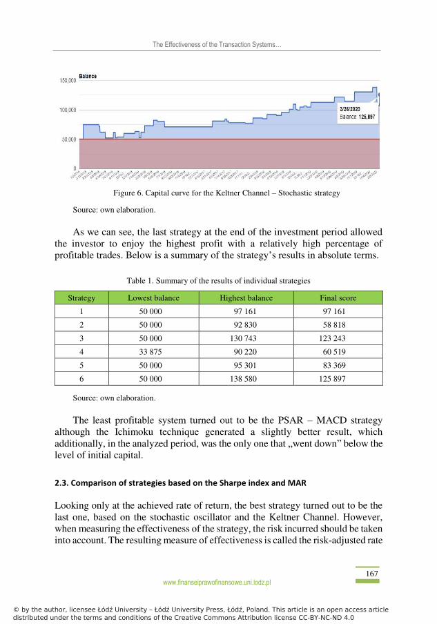
Figure 6. Capital curve for the Keltner Channel – Stochastic strategy


As we can see, the last strategy at the end of the investment period allowed

the investor to enjoy the highest profit with a relatively high percentage of

profitable trades. Below is a summary of the strategy’s results in absolute terms.

Table 1. Summary of the results of individual strategies

Strategy Lowest balance Highest balance Final score

1 50 000 97 161 97 161

2 50 000 92 830 58 818

3 50 000 130 743 123 243

4 33 875 90 220 60 519

5 50 000 95 301 83 369

6 50 000 138 580 125 897


The least profitable system turned out to be the PSAR – MACD strategy

although the Ichimoku technique generated a slightly better result, which

additionally, in the analyzed period, was the only one that „went down” below the

level of initial capital.

2.3. Comparison of strategies based on the Sharpe index and MAR

Looking only at the achieved rate of return, the best strategy turned out to be the

last one, based on the stochastic oscillator and the Keltner Channel. However,

when measuring the effectiveness of the strategy, the risk incurred should be taken

into account. The resulting measure of effectiveness is called the risk-adjusted rate


168



of return. This concept includes, among others, Sharpe meter. The higher the ratio,

the better, as the strategy generated a higher rate of return per risk unit. The Sharpe

measure is defined by the following formula [Ormaniec 2019: 32]:

Sh = r−rfσ ,

where:

r – the average rate of return on the portfolio,

rf – risk-free rate of return,

σ – standard deviation of rates of return.

The value of the indicator itself after adjusting for the incurred risk is not

enough to assess the quality of individual strategies, but only serves to compare

them [Jajuga 2015: 257]. The indicator is the most frequently used measure of the

management efficiency of investment funds, but it can also be successfully used

to evaluate transaction systems.

In the study, the average rate of return on the portfolio was taken as the

average of the annual rates of return over the full 5 years (thus the first quarter of

2020 was omitted). The most frequently considered risk-free rate is the yield on

10-year treasury bonds. In the analyzed period, the average profitability of

German „10-year-olds” fluctuated around 0%, therefore, the Sharpe index was

adjusted to the quotient of the average annual rates of return and their standard

deviation. The results are presented in the table below.

Table 2. Sharpe index for the analyzed transaction systems

Strategy Average annual rate of return Standard deviation Sharpe Ratio

1 17,3% 30,2% 0,57

2 11,1% 26,1% 0,43

3 25,2% 41,1% 0,61

4 28,2% 72,4% 0,39

5 14,5% 31,0% 0,47

6 21,6% 10,9% 1,98


The most effective strategy turned out to be the one based on the Keltner

Channel and the stochastic oscillator, and the least effective strategy was number

4, i.e. the Japanese Ichimoku technique.




Another indicator that can be used to compare transaction systems is MAR

(Managed Account Ratio). We calculate it as the quotient of two values [www4,

accessed 24.04.2020]:

MAR = CAGR % / maxDD %

CAGR is nothing more than the rate of capital growth calculated in relation

to the initial value and smoothed to annual periods. The denominator of the

equation is the maximum percentage of capital drawdown, understood as the

distance between the local maximum and minimum on the capital curve during

the entire investment period [www9, accessed 24.04.2020]. During the 21

analyzed quarters, the highest MAR was characteristic for strategy no. 3, i.e. based

on the Bollinger bands and the RSI oscillator. Strategies 5 and 6 also showed

a high reading, while strategy 2 (Parabolic SAR along with MACD) was the

worst. The table below presents a list of individual systems.

Table 3. MAR coefficient for the analyzed transaction systems

Strategy CAGR maxDD MAR

1 13,5% 16,4% 0,82

2 3,1% 18,8% 0,17

3 18,7% 15,3% 1,23

4 3,7% 26,7% 0,14

5 10,2% 9,8% 1,04

6 19,2% 22,7% 0,85


Based on the data contained in the above tables, it can be concluded that the

best strategies turned out to be strategies no. 3 and 6, while the least effective are

strategies no. 2 and 4.

Interestingly, the Sharpe and MAR ratios provided information in line with

the final balances on the investor’s account.

3. PASSIVE STRATEGY – „BUY AND HOLD”

An alternative to active investment strategies that use technical analysis is

a passive long-term investment strategy based mainly on fundamental analysis.

Unfortunately, in the case of stock indices, comparing them is not as easy as it

may seem. Well, long-term maintenance of positions on futures or CFDs would


170



be associated with very large capital slips. Moreover, the costs of holding

positions on contracts for difference would significantly reduce the investor’s

possible profits. Therefore, when it comes to passive strategies, a better solution

is, for example, investments in ETFs, on which active trading is not profitable

because both when buying and selling, commissions of about 0.30% are charged

[www10, accessed 27.04.2020].

Despite the slightly different specificity of the instruments corresponding to

a given strategy, it is worth looking at how a buy and hold investment would look

like in the same investment horizon against the background of previously tested

trading systems. The analysis was carried out on the largest, in terms of assets,

ETF replicating the DAX index, i.e. iShares Core DAX UCITS ETF, in which all

dividends are reinvested [www11, accessed 27.04.2020].

Assuming that the investor purchased the participation units at the beginning

of 2015, they had to pay 95 euros for each. During the course of the investment,

their value dropped four times below the purchase price, reaching the lowest level

of EUR 82 (–13.7% of the capital invested) in the March panic in 2020. The

highest return could have been achieved in January 2018 and February 2020, when

the rate was close to EUR 131 (+37.9%). If the investor decided to sell the units

at the end of March 2020, they would receive EUR 95 for each of them, which is

the same price as at the start of the investment, after nearly 16% rebound from this

year’s minima. In this case, the MAR coefficient would oscillate around 0.

Let us consider one more scenario that ignores the first quarter crash of this

year. The unit price (including dividends paid and reinvested) at the end of 2019

was EUR 126.70. With a CAGR of 5.9% and a maximum 2015–2016 capital draw

of 25.8%, the MAR index would show a reading of 0.23. Sharpe’s measure,

calculated in the same way as for the 6 tested strategies for a period of full five

years, shows the value of 0.43.

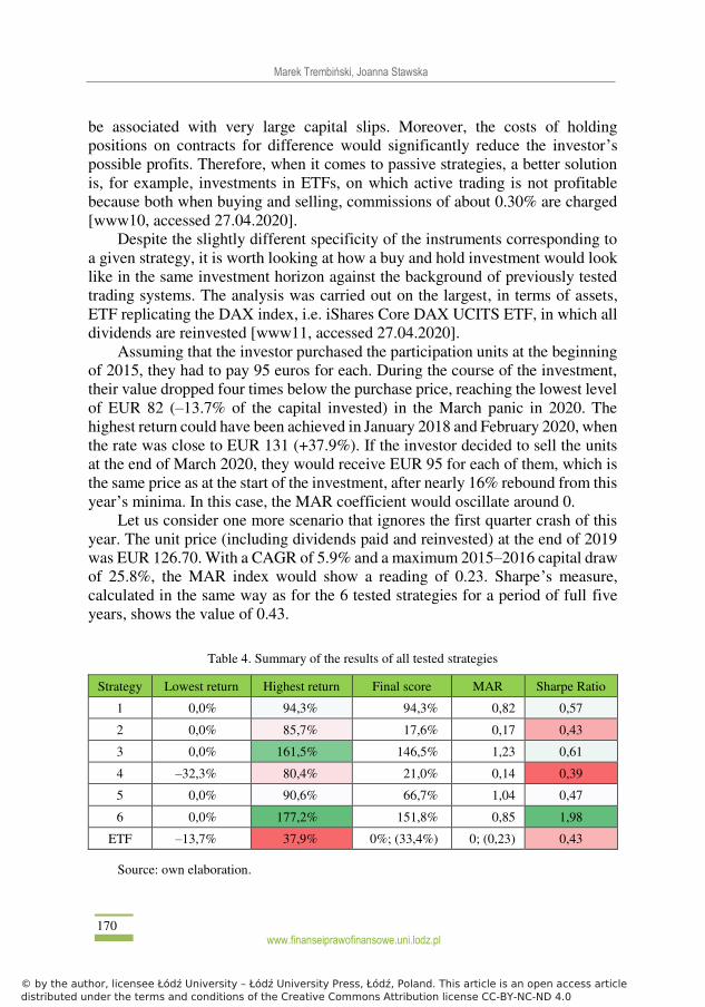
Table 4. Summary of the results of all tested strategies

Strategy Lowest return Highest return Final score MAR Sharpe Ratio

1 0,0% 94,3% 94,3% 0,82 0,57

2 0,0% 85,7% 17,6% 0,17 0,43

3 0,0% 161,5% 146,5% 1,23 0,61

4 –32,3% 80,4% 21,0% 0,14 0,39

5 0,0% 90,6% 66,7% 1,04 0,47

6 0,0% 177,2% 151,8% 0,85 1,98

ETF –13,7% 37,9% 0%; (33,4%) 0; (0,23) 0,43





Data with a summary of the active and passive strategies are presented in

Table 4.

For ETF investments, figures in parentheses assume unit sales on December

31, 2019.

3.1. Research summary

The data presented in Table 3 show that during the research period, only two

strategies (Ichimoku and ETF) would produce negative returns at the worst

possible end of the investment. At the best moment, the „passive” investment achieved the lowest result. Looking at the final balance at the end of 2019, as

many as 4 systems based on technical analysis were more effective than the „buy

and hold” strategy, and at the end of the first quarter of 2020 – all of them. When

analyzing the measures of management quality, it turns out that taking into

account the 21 quarters, the passive strategy was characterized by the lowest MAR

index. The Sharpe’s measure is also relatively weak compared to the 4 leading

strategies.

In addition, each of the systems achieved a positive rate of return, and losses

were only reduced by the previously generated surpluses in as many as 5 out of 6

examined cases. The average profit for a single strategy is EUR 41,500 or 1,660

points.

SUMMARY

The aim of the article was to test the effectiveness of trading systems built on the

basis of technical analysis in 2015–2020 on the DAX stock exchange index. This

goal has been achieved, which is confirmed by the results of the research that

allow to evaluate the effectiveness of the transaction systems under study in 2015–2020. On the basis of the transactions carried out, it can be concluded that the

technical analysis works in practice and on its basis it is justified to construct

investment strategies that can bring profits in the long term while maintaining an

appropriate level of risk. It is true that the percentage of unprofitable positions was

relatively high, but the generated sell signals made it possible to cut losses quite

quickly. As a result, only one of all analyzed capital curves fell below the level of

initial capital during the investment period. It is worth noting that additional

verification of more parameters for each oscillator, channel or moving average, as

well as changing the time interval or other tool combinations, would probably

improve the performance of the systems. A comparison against the background of

passive investment, both in terms of the quality of portfolio management and the

achieved rates of return, is definitely in favor of active strategies. However, due


172



to the different specifics of the instruments, it should be approached with a lot of

caution.

In the light of the conducted research, it is worth emphasizing that there is no

single best transaction system that will always bring above-average rates of return,

regardless of the current market situation. Financial markets are characterized by

high dynamics of changes, therefore, a strategy that has been successful in recent

years may not necessarily prove successful in the future. Moreover, the obtained

results indicate that the evaluation of the effectiveness of a given strategy differs

depending on the measures used.

Technical analysis is not without its drawbacks. Perhaps it does not discount

all information, but only the well-known or foreseeable by the market. The

simulations carried out prove that technical analysis is an effective tool for risk

management and, in combination with fundamental analysis, increases the

probability of success. It is clear that history does not always have to repeat itself,

but the psyche of investors has remained unchanged for years.

BIBLIOGRAPHY

Bąk B., 2015, Skuteczność techniki Ichimoku na przykładzie kontraktów terminowych na indeks WIG20, Uniwersytet Marii Curie-Skłodowskiej, Wydział Ekonomiczny, Lublin.

Borowski K., 2001, Technika Ichimoku (renesans japońskiej techniki inwestowania), „Studia i Prace

Kolegium Zarządzania i Finansów”, z. 19.

Borowski K., 2017, Analiza techniczna. Średnie ruchome wskaźniki i oscylatory, Difin, Warsaw.

Borowski K., 2018, Metody inwestowania na rynkach finansowych, Difin, Warsaw.

Borowski K., 2019, Efficiency and stability of trading systems based on plain, exponentially and

linearly weighted moving averages, „Annales Universitatis Mariae Curie-Skłodowska. Section

H–Oeconomia”, vol. 53, no. 4.

Czekała M., 1997, Analiza fundamentalna i techniczna, Wydawnictwo Akademii Ekonomicznej im.

Oskara Langego, Wrocław. Elder A., 2018, Zawód Inwestor Giełdowy. Nowe ujęcie, XTB, Poznań.

Elliott N., 2007, Ichimoku Charts. An introduction to Ichimoku Kinko Clouds, Harriman House.

Etzkorn M., 1999, Oscylatory, WIG Press, Warsaw.

Frierdich M., 2013, Hedge Funds. Die Konigsklasse der Investments, FBV, Monachium.

Jabłoński B., 2006, Innowacyjna strategia ograniczająca ryzyko walutowe, Uniwersytet Ekono-

miczny w Katowicach, Katowice.

Jajuga K., 2015, Inwestycje, Wydawnictwo Naukowe PWN, Warsaw.

Kochan K., 2009, Forex w praktyce, Helion, Gliwice.

LeBeau C., Lucas D., 1998, Komputerowa analiza rynków terminowych, WIG PRESS, Warsaw.

Murphy J., 1995, Analiza techniczna, WIG PRESS, Warsaw.

Murphy J., 2017, Analiza techniczna rynków finansowych, Admiral Markets, Poznań.

Nowakowski J., 2003, Normalizacja wskaźników analizy technicznej, „Studia i Prace Kolegium Za-

rządzania i Finansów”, z. 29.

Ormaniec T., 2019, Możliwość osiągania ponadprzeciętnych stóp zwrotu na podstawie informacji

o sprzedaży oraz umorzeniach jednostek uczestnictwa w otwartych funduszach inwestycyj-

nych, „Studia i Prace Kolegium Zarządzania i Finansów. Zeszyt Naukowy”, nr 173.




Oziemczuk K., 2011, Ichimoku. Japońska strategia inwestycyjna, Bullet Books, Warsaw.

Pająk A., 2013, Dochodowość inwestycji w kontrakty terminowe na akcje w Polsce, Wydawnictwo

Adam Marszałek, Toruń.

Rockefeller B., 2012, Analiza techniczna dla bystrzaków, Wydawnictwo Septem.

Słupek T., 2001, Analiza techniczna. Wprowadzenie, Dom Wydawniczy ABC, Cracow.

Other Internet Sources:

Cennik Biura Maklerskiego ING Banku Śląskiego, www.ing.pl/indywidualni/inwestycje-i-

oszczednosci/inwestycje-gieldowe/etf [accessed 27.04.2020].

[www1] www.3sigma.com/whats-so-special-about-3-sigma [accessed 03.03.2020].

[www2] www.admiralmarkets.pl/education/articles/forex-indicators/parabolic-sar-forex

[accessed 28.02.2020].

[www3] www.admiralmarkets.pl/education/articles/forex-indicators/wskaznik-cci

[accessed 24.04.2020]

[www4] www.blogi.bossa.pl/2008/05/30/miary-oplacalnosci-i-ryzyka-transakcji/

[accessed 24.04.2020].

[www5] www.blogi.bossa.pl/2011/04/22/subiektywizm-analizy-technicznej/

[accessed 02.02.2020].

[www6] www.comparic.pl/category/analizy/indeksy/dax/ [accessed 10.04.2020].

[www7] www.comparic.pl/parabolic-sar-przewodnik-od-tradeciety/ [accessed 30.03.2020].

[www8] www.comparic.pl/tradeciety-wstega-bollingera-najlepszy-wskaznik-wielu-powodow/

[accessed 2.04.2020].

[www9] www.fxmag.pl/artykul/obsuniecie-kapitalu-jak-interpretowac-drawdown

[accessed 24.04.2020].

[www10] www.ing.pl/ individual/investment-and-savings/investment-gieldowe/etf

[accessed 27.04.2020].

[www11] www.justetf.com/en/how-to/dax-etfs.html [accessed 27.04.2020].

[www12] www.parkiet.com/artykul/1432239.html [accessed 27.03.2020].

[www13] www.parkiet.com/artykul/1433930.html [accessed 15.04.2020].

[www14] www.sii.org.pl/static/img/004366/Podstawy_analizy_Ichimoku.pdf

[accessed 15.03.2020].

[www15] www.thebalance.com/how-to-day-with-trade-keltner-channels-4051613

[accessed 20.03.2020].

[www16] www.tms.pl/wskazniki-trendu [accessed 27.02.2020].

[www17] www.tradersarea.pl/kanal-donchiana/[accessed 28.03.2020].

List of abbreviations:

ADX – Average Directional Movement Index

ATR – Average True Range

CCI – Commodity Channel Index

CFDs – Contracts For Difference

DAX – Deutscher Aktienindex

DI+ – (Directional Indicator +)

DI– – (Directional Indicator –)

DMI – Directional Movement Index

ETF – Exchange traded fund

MAR – Managed Account Ratio.

MACD – Moving Average Convergence/Divergence


174



MAR – Managed Account Ratio

PSAR – Parabolic Stop and Reversal

SAR – Parabolic Stop and Reversal

SMA – Simple Moving Average

RSI – Relative Strength Index.

Przyjęto/Accepted: 10.11.2020 Opublikowano/Published: 31.12.2020


Powered by TCPDF (www.tcpdf.org)

http://www.tcpdf.org

9337-9181.pdf - CEJSH

Documents

Transcript of 9337-9181.pdf - CEJSH